A Testable Three-Layer Retained-State Framework for Intelligent Energy Systems: Metrics, Public Experimental Validation, and Cross-Scale Applications

Abstract

This paper proposes a testable three-layer retained-state framework for intelligent energy systems grounded in mem-element theory. The framework distinguishes constitutive physical memory (Layer I), distributed circuit/converter memory (Layer II), and functional operational memory (Layer III) while preventing the indiscriminate classification of any history-dependent model as a mem-system. A retained variable is admissible only when it satisfies persistence, trajectory dependence, observable engineering consequence, and positive relevance beyond an instantaneous reference. Quantitative trajectory-separation, retained-state relevance, and engineering-gain indices, together with observability and falsification conditions, convert the framework from a taxonomy into a testable methodology. Layer I was partially validated using 636 experimental discharge cycles from four cells in the public NASA Ames PCoE Li-ion Battery Aging Dataset. Across 120 cycle–disjoint within-cell pairs matched at closely similar voltages, currents, temperatures, and local slopes, the median future-trajectory separation ($M_{\mathrm{T}\mathrm{S}}$) was 0.0688, the noise-normalized separation ($M_{\mathrm{N}\mathrm{S}}$) was 20.13, and the remaining-discharge duration differed by 150.7 s. Leave-one-battery-out prediction yielded positive retained-state relevance ($M_{\mathrm{R}\mathrm{I}}$ = 0.159 with a random-forest model; 95% bootstrap interval: 0.121–0.194). Two reduced-order cross-scale applications were then used for Layers II and III. In resonant wireless EV charging, retained-state augmentation reduced the efficiency RMSE by 29.9–32.2% and the current MAE by 27.5–27.9% in disturbed scenarios. In EV charging/V2G scheduling, history-aware operation reduced the charging cost by 3.3%, the degradation proxy by 12.0%, thermal-limit violations by 27.3%, and aggressive cycling by 17.2% while accepting lower peak reduction and V2G revenue. Same-information controls produced identical numerical outputs to the structured models by construction, showing that the framework’s novelty lies in admissibility, falsifiability, and cross-scale interpretation rather than privileged input information. The NASA study provides bounded public-experimental-data validation of Layer I; Layers II and III remain proof-of-concept demonstrations.

1. Introduction

Modern energy systems increasingly exhibit retained-state effects: magnetic hysteresis, thermal accumulation, electrochemical degradation, resonant-state evolution, and operational decision history can alter efficiency, stress, flexibility, and lifetime even when present inputs appear similar [1,2].

Mem-element theory provides a rigorous device- and circuit-level origin for such behavior through memristive, memcapacitive, and meminductive formulations whose present response depends on internal state and prior excitation [3,4]. Related retained-state effects also appear in batteries, power converters, wireless charging, smart grids, and adaptive energy management [5,6].

The unresolved problem is not whether history is used but when that history carries a distinct engineering meaning. State-space models, model predictive control, reinforcement learning, digital twins, and cyber-physical systems already represent dynamic states and historical information [6,7]. They do not, however, provide a bounded cross-scale rule for distinguishing constitutive physical memory, distributed converter memory, and functional operational memory, nor do they specify when a memory-aware interpretation should be rejected as unnecessary.

This paper therefore proposes a falsifiable three-layer framework. A retained state is admitted only when it satisfies four inclusion criteria—persistence, trajectory dependence, observable consequence, and modeling or decision gain—and when it can be assigned to a declared layer. Trajectory-separation, retained-state relevance, and engineering-gain indices, together with observability and rejection conditions, make the framework testable rather than purely taxonomic.

The contribution is fivefold: (1) a bounded three-layer retained-state formalism; (2) quantitative inclusion and falsification tests that distinguish memory-aware behavior from arbitrary state augmentation; (3) a compact public-experimental-data validation of Layer-I retained-state relevance using the NASA Ames PCoE Li-ion Battery Aging Dataset; (4) a same-information control showing explicitly that numerical improvement originates from retained-state information, whereas the framework adds classification and interpretability; and (5) two cross-scale proof-of-concept applications in resonant wireless EV charging and history-aware EV/V2G scheduling.

2. Formal Definition and Inclusion Criteria for Memory-Aware Energy Systems

To prevent conceptual overextension, the framework treats memory-aware behavior as a testable retained-state property rather than a synonym for nonlinearity, state dependence, or the use of historical samples.

A system is memory-aware when its observable response (y(t)) cannot be adequately described by instantaneous input (u(t)) and conventional state (z(t)) alone but depends on a retained state (x_m(t)) shaped by prior excitation, operation, or decisions:

$$x_m\left(t+1\right)=F_m\left(x_m\left(t\right),u\left(t\right),z\left(t\right),\theta \right)$$

$$y\left(t\right)=G\left(u\left(t\right),z\left(t\right),x_m\left(t\right),\theta \right)$$

Here, θ denotes the model parameters. The retained state may be physical, distributed across a converter, or operationally stored by a supervisory system.

Four jointly necessary criteria are applied: (1) state retention over a declared time scale; (2) trajectory dependence, such that similar u(t) and z(t) can yield different y(t) when x_m(t) differs; (3) an observable consequence for efficiency, stress, degradation, flexibility, or control; and (4) positive predictive, diagnostic, interpretive, or decision gain relative to an instantaneous reference. Failure of any criterion rejects the memory-aware label.

2.1. Quantitative Retained-State Metrics

To convert the inclusion criteria into testable quantities, let ${\mathbf{y}}_A$ and ${\mathbf{y}}_B$ denote the output trajectories obtained at approximately identical instantaneous inputs and conventional states but from different prior histories. The normalized trajectory-separation index is

$$M_{\mathrm{T}\mathrm{S}}={\displaystyle \frac{\parallel {\mathbf{y}}_A-{\mathbf{y}}_B{\parallel }_2}{{\parallel {\mathbf{y}}_A\parallel }_2+{\parallel {\mathbf{y}}_B\parallel }_2+ \epsilon }}$$

Because a small normalized difference may still be significant in low-noise measurements, the complementary noise-normalized separation is

$$M_{\mathrm{N}\mathrm{S}}={\displaystyle \frac{\sqrt{\frac{1}{N}{\displaystyle {\sum }_{j=1}^N}{\left(y_{A,j}-y_{B,j}\right)}^2}}{{\sigma }_y}}={\displaystyle \frac{\parallel {\mathbf{y}}_A-{\mathbf{y}}_B{\parallel }_2}{\sqrt{N}\hspace{0.17em}{\sigma }_y}}$$

where $N$ is the number of trajectory samples, ${\sigma }_y$ is the declared per-sample measurement or simulation-noise scale, and $\epsilon$ > 0 prevents division by zero.

Retained-state relevance is evaluated against the same-data instantaneous reference as

$$M_{\mathrm{R}\mathrm{I}}=1-{\displaystyle \frac{E_{\mathrm{a}\mathrm{u}\mathrm{g}}}{E_{\mathrm{i}\mathrm{n}\mathrm{s}\mathrm{t}}+\epsilon }}$$

where the same out-of-sample error measure (MSE, RMSE, or MAE) is used for both models. Positive values indicate retained-state relevance; non-positive values indicate no explanatory gain. For control and scheduling objectives, the engineering-gain component for metric q is

$$M_{\mathrm{E}\mathrm{G},q}=\left\{\begin{array}{ll}{\displaystyle \frac{J_{\mathrm{i}\mathrm{n}\mathrm{s}\mathrm{t},q}-J_{\mathrm{a}\mathrm{u}\mathrm{g},q}}{\left|J_{\mathrm{i}\mathrm{n}\mathrm{s}\mathrm{t},q}\right|+\epsilon }},& \mathrm{lower}\text{-}\mathrm{is}\text{-}\mathrm{better} \mathrm{metric},\\ {\displaystyle \frac{J_{\mathrm{a}\mathrm{u}\mathrm{g},q}-J_{\mathrm{i}\mathrm{n}\mathrm{s}\mathrm{t},q}}{\left|J_{\mathrm{i}\mathrm{n}\mathrm{s}\mathrm{t},q}\right|+\epsilon }},& \mathrm{higher}\text{-}\mathrm{is}\text{-}\mathrm{better} \mathrm{metric}.\end{array}\right.$$

Positive $M_{\mathrm{E}\mathrm{G},q}$ denotes improvement. Multi-objective gains are reported as a vector rather than collapsed into an arbitrary scalar.

A system is classified as quantitatively memory-aware only when $M_{\mathrm{T}\mathrm{S}}$ exceeds a predeclared uncertainty-dependent threshold, $M_{\mathrm{N}\mathrm{S}}$ exceeds the declared noise criterion where available, $M_{\mathrm{R}\mathrm{I}}$ is positive under out-of-sample or perturbation testing, and the retained variable has a physically or operationally interpretable origin. Failure of any mandatory condition rejects the memory-aware label for that application.

2.2. Formal Properties and Falsification Conditions

Definition 1 (Admissible Retained State).

A variable ($x_m$) is an admissible retained state only if it satisfies four jointly necessary conditions: persistence over a declared time scale; dependence on prior excitation or prior decisions; measurable influence on an engineering output; and non-redundancy with respect to the instantaneous-state vector. After conditioning on present inputs and conventional states, inclusion of $x_m$ must produce positive out-of-sample retained-state relevance, $M_{\mathrm{R}\mathrm{I}}$ > 0.

Proposition 1 (Non-Equivalence to Arbitrary State Augmentation).

The existence of an augmented state vector does not by itself establish memory-aware behavior. A state-augmented model qualifies under the proposed framework only when two trajectories, A and B, can approach the same instantaneous operating point while producing distinguishable outputs, $M_{\mathrm{T}\mathrm{S}}$ > ${\tau }_{\mathrm{T}\mathrm{S}}$, and when the retained variable provides positive out-of-sample explanatory or engineering gain. Therefore, ordinary state augmentation is a necessary representation mechanism in many cases, but it is not a sufficient classification criterion.

Proof. 

If $M_{\mathrm{T}\mathrm{S}}$ ≤ ${\tau }_{\mathrm{T}\mathrm{S}}$, the two histories are observationally indistinguishable at the declared resolution and the retained-state interpretation is unsupported. If $M_{\mathrm{R}\mathrm{I}}$ ≤ 0, the additional variable does not improve explanation beyond the instantaneous reference. If the variable has no physical or operational interpretation, the augmentation may be statistically useful but cannot be assigned to one of the three retained-state layers. The three tests jointly exclude arbitrary historical features from the framework. □

Proposition 2 (Layer Projection Consistency).

Let $x_m^{\left(1\right)}$, $x_m^{\left(2\right)}$, and $x_m^{\left(3\right)}$ denote the retained states at the physical, converter, and operational layers. A cross-layer claim is admissible only if each asserted projection, $P_{12}$ $x_m^{\left(1\right)}$ → $x_m^{\left(2\right)}$ or $P_{23}$: $x_m^{\left(2\right)}$ → $x_m^{\left(3\right)}$, is linked to an observable engineering consequence and preserves the relevant trajectory distinction. A higher-layer memory state may exist without a one-to-one lower-layer realization, but the manuscript must not claim physical constitutive equivalence unless the corresponding lower-layer mapping is identified and validated.

Proposition 3 (Observability Requirement).

For a latent retained state ($x_m$) to support prediction or control, it must be locally observable or practically reconstructible from available measurements over a finite horizon. For a nonlinear model, $x_m$(t + 1) = F($x_m$(t),u(t),z(t)) and y(t) = G($x_m$(t),u(t),z(t)), this requires the local observability map generated by successive output sensitivities to have full column rank in the neighborhood of interest or an equivalent empirical identifiability test to demonstrate bounded estimation error.

In practical implementations, latent retained states may be reconstructed using an extended or unscented Kalman filter, moving-horizon estimation, a nonlinear Luenberger-type observer, or a physics-informed estimator. The selected estimator must be validated using residual whiteness, bounded state-estimation error, and robustness to parameter perturbation. If the state cannot be reconstructed with acceptable uncertainty, its use is restricted to qualitative interpretation and it must not support closed-loop or deployment-level claims.

Falsification rule: The framework should not be used when any of the following conditions holds: (i) trajectory separation is below the declared noise-dependent threshold; (ii) retained-state relevance is non-positive under out-of-sample testing; (iii) the additional state is observationally non-identifiable; or (iv) no engineering consequence can be associated with the retained history. In these cases, conventional state-space, control, or data-driven modeling is sufficient and the memory-aware label should be rejected.

2.3. Relation to Conventional State-Space Modeling

Conventional state-space models remain the mathematical substrate. The present framework adds an engineering classification: it singles out a state only when the inclusion criteria and quantitative tests are met, assigns it to a physical, converter, or operational layer, and rejects the interpretation when a conventional model provides the same explanatory and decision value without that structure. It therefore complements rather than replaces control, optimization, digital-twin, reinforcement-learning, and battery models.

2.4. Hierarchical State Projection Across Memory Layers

The three layers are linked by state projections rather than by an assumed formal equivalence.

At the physical layer (Layer I), retained-state behavior is represented by an internal physical memory state:

$$x_m^{\left(1\right)}\left(t+1\right)=F_1\left(x_m^{\left(1\right)}\left(t\right),u\left(t\right),{\theta }_1\right)$$

where $x_m^{\left(1\right)}$ denotes physically grounded memory variables, such as trapped charge, ionic distribution, magnetic state, dielectric polarization, thermal burden, or electrochemical degradation, and u(t) is the external excitation.

At the circuit and converter layer (Layer II), the effective retained-state behavior depends not only on converter-level dynamics but also on the aggregated influence of Layer-I physical memory:

$$x_m^{\left(2\right)}\left(t+1\right)=F_2\left(x_m^{\left(2\right)}\left(t\right),x_m^{\left(1\right)}\left(t\right),u\left(t\right),z\left(t\right),{\theta }_2\right)$$

where $x_m^{\left(2\right)}$ represents distributed dynamic memory, such as switching history, resonant-state evolution, magnetic operating-point history, and thermal-circuit interaction. Here, z(t) denotes conventional measurable system states.

At the system-level adaptive-intelligence layer (Layer III), retained-state behavior incorporates supervisory operational history and decision memory:

$$x_m^{\left(3\right)}\left(t+1\right)=F_3\left(x_m^{\left(3\right)}\left(t\right),x_m^{\left(2\right)}\left(t\right),d\left(t\right),u\left(t\right),z\left(t\right),{\theta }_3\right)$$

where $x_m^{\left(3\right)}$ represents operational memory such as charging history, storage-utilization records, dispatch history, adaptive policy state, or retained optimization context, and d(t) denotes decision-state history.

Projection consistency requires that each higher-layer retained state preserve information relevant to its observable output. For adjacent layers ℓ and ℓ + 1, the projection Pℓ → ℓ + 1 is informative when

$$I \left(x_m^{\left(\mathcal{l}\right)};y^{\left(\mathcal{l}+1\right)}\mid z,u\right)>0, {\displaystyle \frac{\mathsf{\partial }{y}^{\left(\mathcal{l}+1\right)}}{\mathsf{\partial }{x}_m^{\left(\mathcal{l}\right)}}}\ne 0$$

where I denotes conditional mutual information. The first condition applies to stochastic or data-driven settings; the sensitivity condition is its local deterministic analogue over the declared operating region.

The hierarchy is not assumed to be invertible. Recoverability of a lower-layer state from higher-layer measurements requires local observability of the augmented model. For a differentiable discrete-time system, this can be assessed through the rank of the augmented observability matrix constructed from the output map and repeated Lie or Jacobian propagation. Failure of the rank condition does not invalidate the layer classification, but it requires the retained state to be reported as latent and prevents claims of unique physical identification.

2.5. Strict, Mem-Inspired, and Functional Memory Interpretations

The framework distinguishes three claims, summarized in Table 1: strict mem-systems have memory-dependent constitutive relations; mem-inspired state-based models use retained states to explain trajectory-dependent circuit or converter behavior; and functional memory-aware systems use retained operational information in scheduling, adaptation, or coordination without being literal mem-elements.

Table 1. Inclusion logic for memory-aware interpretations in intelligent energy systems.

Appropriate Claim	Main Criterion	Typical Retained State	Interpretation Level
Physically grounded mem-element or mem-system model	Constitutive relation depends on internal state and prior excitation	Physical internal state such as ionic distribution, charge trapping, magnetic state, or dielectric state	Strict mem-system
State-augmented memory-aware model	Retained trajectory affects observable circuit or converter behavior	Distributed converter, resonant, magnetic, thermal, or switching-history state	Mem-inspired state-based model
Conceptual and modeling framework for adaptive energy operation	Retained information affects system-level decision or flexibility	Operational history, usage trajectory, control memory, stress accumulation, or decision state	Functional memory-aware system

2.6. Boundary Against Overgeneralization

Three cases are excluded: static nonlinearity fully determined by current variables; controllers that merely store previous samples without a decision-relevant retained state; and high-level optimization labeled mem-element-based without explicit states, trajectory linkage, and observable consequence. These exclusions preserve the boundary between constitutive memory, state-based modeling, and functional analogy.

3. Relationship to Existing Modeling and Control Frameworks

Many established energy-system methodologies already incorporate dynamic states, historical measurements, forecasts, and adaptive decision variables. The contribution of the present framework is therefore not the introduction of state retention itself but the classification of retained states according to their physical, converter-level, and operational meaning.

To make this positioning explicit, Table 2 compares the information retained by the principal modeling and control approaches, the strengths they already provide, and the narrower role assigned to the proposed framework.

Table 2. Comparison between proposed memory-aware framework and existing modeling, control, and energy-system approaches.

Added Role of Proposed Framework	Limit for This Question	Main Strength(s)	Typical Retained Information	Established Approach
Assigns admissible states to physical, converter, or operational layers	Does not classify the engineering meaning of retained states across scales	Rigorous dynamics, observability, and transient analysis	Electrical, magnetic, thermal, and switching states	State-space and nonlinear converter models
Separates physical burden, converter stress, and operational memory	Uses history effectively without distinguishing memory-specific meaning	Constraint-aware scheduling and control	Predicted trajectories, constraints, and cost states	Model predictive and optimal control
Separates functional decision memory from strict mem-system claims	Algorithmic memory may lack physical interpretation	Data-driven adaptation	Policy, value, recurrent state, and experience	Reinforcement learning and adaptive control
Adds trajectory, relevance, observability, and falsification tests	May retain many histories without relevance or rejection tests	Monitoring, coordination, and what-if analysis	Sensor histories, digital states, and degradation indicators	Cyber-physical systems and digital twins
Links physical states to higher-layer consequences without replacing domain models	Usually localized to a component or domain	Mature domain-specific physical models	SoC, SoH, temperature, cycle, hysteresis, and relaxation states	Battery, hysteresis, and thermal-memory models
Defines functional Layer-III memory without literal mem-element claims	Operational history is rarely linked explicitly to device/converter memory	Scheduling, demand response, and grid support	Load, price, storage, and dispatch histories	Smart-grid and energy management methods
Provides admissibility metrics, observability, same-information control, and a rejection rule	Not a substitute for domain-specific models	Cross-scale classification and testability	Physical, converter, and operational retained states	Proposed three-layer framework

Table 2 positions the framework against established methods. Its contribution is neither a new state estimator nor a replacement for domain models but a disciplined rule for assigning retained states to layers, testing relevance, requiring observability, and rejecting the classification when trajectory separation is below uncertainty or when a simpler augmented model gives the same engineering conclusion.

4. Mem-Element Foundations and Technology Maturity

4.1. Circuit-Theoretic Foundations

Ideal resistors, capacitors, and inductors are memoryless, whereas practical devices can exhibit internal-state dependence through charge trapping, ionic transport, magnetic hysteresis, dielectric relaxation, thermal inertia, or degradation [7,8,9,10]. Mem-element theory formalizes this distinction by allowing terminal response to depend on both present excitation and an evolving internal state.

Memristive systems use state-dependent voltage–current relations; memcapacitive and meminductive systems analogously introduce state-dependent charge–voltage and flux–current relations [10,11,12,13,14,15]. The defining feature is not nonlinearity alone but path dependence: two trajectories reaching similar terminal conditions can produce different responses because the internal states differ [16,17,18,19,20].

Generalized mem-systems are therefore the appropriate foundation for this work. At higher scales, the same structural logic may appear as distributed converter or operational memory, but the claim changes from constitutive to mem-inspired or functional. The three-layer framework preserves this distinction rather than treating every dynamic energy system as a literal network of mem-elements.

4.2. Technology Maturity and Integration Limits

Memristive devices—such as RRAM, CBRAM, phase-change, and ferroelectric resistive structures—are the most experimentally mature Layer-I realizations [21,22,23,24]. Memcapacitive behavior is reported in ferroelectric and dielectric structures, while meminductive behavior is typically embedded in magnetic-core, saturable, or hysteretic coupled systems [25,26,27,28].

Direct high-power integration remains limited by variability, endurance, stochastic switching, thermal stability, scalability, and the difficulty of isolating ideal memcapacitive or meminductive elements [29,30,31,32]. Near-term energy applications are therefore more credible as physically grounded device models, memory-aware converter observers, and neuromorphic or history-aware supervisory functions than as wholesale replacements of established power hardware [32,33,34,35].

5. Application Domains Across Scales

The framework is applied only where the retained state changes an observable engineering conclusion. Across the three layers, the relevant question is not whether a model contains history but whether two trajectories that converge to similar instantaneous conditions remain distinguishable in efficiency, stress, lifetime, flexibility, or control action.

5.1. Physical and Component Memory

Layer I includes charge trapping, ionic redistribution, dielectric relaxation, magnetic hysteresis, thermal accumulation, and electrochemical degradation [36,37,38,39]. These mechanisms are physically grounded and may justify strict memristive, memcapacitive, or meminductive descriptions when terminal behavior is governed by an internal state [40,41,42]. Battery integration additionally requires grid compatibility, safety, and environmental constraints; these considerations are represented in the engineering boundary of the framework [43,44,45,46].

5.2. Converter and Charging-Interface Memory

Layer II covers distributed retained states in LLC resonant converters, dual-active-bridge converters, wireless-power-transfer systems, and modular multilevel converters. Representative mechanisms include resonant-tank energy history, transformer-flux bias, circulating-current history, capacitor–voltage imbalance, junction-temperature accumulation, dead-time and modulation history, and coupling or alignment trajectories. The framework is useful only when these retained states produce measurable trajectory separation or improve prediction, diagnosis, or control relative to an instantaneous and a state-augmented reference.

5.3. System-Level and Electric-Mobility Memory

Layer III concerns operational memory in smart grids, battery digital twins, charging platforms, and V2G fleets. Typical retained states include degradation burden, thermal exposure, dispatch history, charging intensity, policy state, and uncertainty carried by AI-enabled digital twins or physics-informed models. This layer also includes memory-augmented reinforcement learning, recurrent decision models, and hybrid physics-informed state-space formulations, provided that their retained variables pass the same admissibility, observability, and falsification tests [36]. These systems are not literal mem-elements. They are classified as functionally memory-aware only when retained information has an identifiable origin, survives out-of-sample testing, and changes a decision-relevant outcome.

5.4. Engineering Usefulness and Decision Rule

The proposed framework should be retained only when three tests are satisfied simultaneously: the trajectory-separation index exceeds a predeclared noise threshold, the retained-state relevance index is positive under validation or perturbation testing, and the engineering-gain index or a vector of physical performance indicators shows non-negligible benefit. If a conventional state-space or state-augmented model provides the same explanatory and decision value, the mem-inspired interpretation should be rejected as unnecessary.

6. A Three-Layer Framework for Memory-Aware Energy Systems

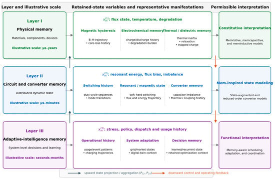
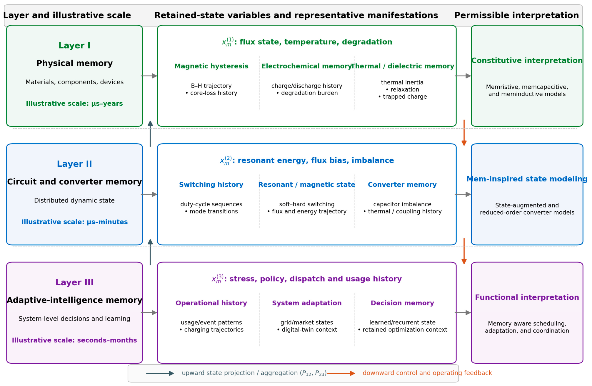
Section 2 defines admissibility and projection; Figure 1 and Table 3 summarize the resulting architecture. Layer I locates physical state retention, Layer II captures distributed circuit and converter trajectories, and Layer III represents decision-relevant operational history.

Figure 1. Three-layer retained-state framework linking physical, circuit/converter, and adaptive-intelligence memory. Upward arrows indicate state projection and aggregation across layers; downward arrows indicate control and operating feedback. The displayed time scales are illustrative and mechanism-dependent.

Table 3. An analytical summary of the proposed three-layer framework, showing how different forms of memory, representative engineering manifestations, and the role of mem-element theory vary across physical, circuit-level, and system-level interpretations.

Possible Role of Mem-Element Theory	Representative Engineering Domains	Typical Phenomena	Type of Memory	Layer
Constitutive modeling of memory-dependent electrical behavior	Nonlinear devices, passive components, magnetic structures, storage materials	Charge trapping, ionic redistribution, magnetic hysteresis, dielectric relaxation, thermal inertia	Material- and device-level memory	Physical memory
State-aware modeling of nonlinear converter and passive-network behavior	Power converters, resonant systems, coupled magnetic structures, charging interfaces	Switching history, resonant-state evolution, magnetic operating-point dependence, thermal-circuit interaction, coupling variation	Dynamic and trajectory-dependent circuit memory	Circuit and converter memory
Conceptual and interpretive framework for adaptive, history-aware intelligent energy systems	Smart grids, energy management systems, electric mobility, distributed energy networks	Charging history, storage trajectories, load evolution, adaptive control, demand response, retained decision states	Operational and decision-level memory	System-level adaptive-intelligence memory

6.1. Layer I: Physical Memory

Layer I includes charge trapping, ionic redistribution, magnetic hysteresis, dielectric relaxation, thermal accumulation, and electrochemical degradation. It supports strict mem-element claims only when terminal behavior is governed by a physically identifiable internal state.

6.2. Layer II: Circuit and Converter Memory

Layer II comprises switching, resonant, magnetic, thermal, and coupling histories distributed across a circuit or converter. These are mem-inspired state-based models: trajectory dependence must be measurable, but no single ideal mem-element is required.

6.3. Layer III: System-Level Adaptive-Intelligence Memory

Layer III comprises charging, dispatch, usage, degradation, policy, and decision histories that change flexibility or control actions. Its interpretation is functional rather than constitutive and is accepted only when the retained information passes out-of-sample relevance and engineering-gain tests.

To consolidate the layer definitions into a single operational view, Figure 1 maps the representative retained states, illustrative time scales, upward state projections, and downward control feedback associated with the three layers.

Table 3 further summarizes the analytical distinctions across the three memory layers, including their characteristic retained states, engineering manifestations, and corresponding interpretations in mem-element theory.

Across the hierarchy, the common principle is retained-state dependence; what changes is physical embodiment, time scale, observability, and permissible claim. State-space, control, optimization, battery, and cyber-physical models remain the implementation tools, while the framework determines when a memory-specific interpretation is justified.

7. Illustrative Simulation-Based Case Studies

7.1. Position, Scope, and Benchmarking Logic of Case Studies

The case studies test one question: can trajectories with similar instantaneous variables produce different engineering outcomes because retained states differ? They are reduced-order proof-of-concept demonstrations, not deployment-level validation or claims that mem-element terminology improves performance.

7.1.1. Benchmarking Logic and Fair-Comparison Principle

Table 4 compares an instantaneous reference with a conventional state-augmented reference and a structured memory-aware interpretation.

Table 4. Fair-comparison logic separating instantaneous, state-augmented, and structured memory-aware models.

Model Class	Information Used	Retained State?	Numerical Role	Scientific Interpretation
Instantaneous reference	Present operating variables only	No	Baseline that suppresses trajectory history	Shows the consequence of omitting retained-state information
State-augmented reference	Present variables plus exactly the same retained states, equations, and coefficients as the structured model	Yes	Same-information numerical control; outputs must match the structured model by construction	Separates the value of additional-state information from the value of the proposed framework
Structured memory-aware model	Same numerical state-augmented model plus inclusion criteria, layer assignment, relevance metrics, observability tests, and falsification rules	Yes	No numerical superiority over the state-augmented control is claimed	Supports the framework only when retained states acquire interpretable, testable, and cross-scale engineering meaning

The latter two use identical states, equations, and coefficients; hence, their numerical outputs are identical by construction. Improvement relative to the instantaneous model is attributable to retained information, while the framework contributes admissibility tests, layer assignment, observability, relevance metrics, and a rejection rule.

7.1.2. Parameter and Validation Boundary

All coefficients are engineering-tuned scenario parameters. Sensitivity analysis tests whether trajectory separation persists under moderate perturbations, but experimental calibration, public-data validation, and comparison with industrial controllers or schedulers remain necessary before deployment-level claims.

7.2. Case Study I: Memory-Aware Resonant Wireless EV Charging

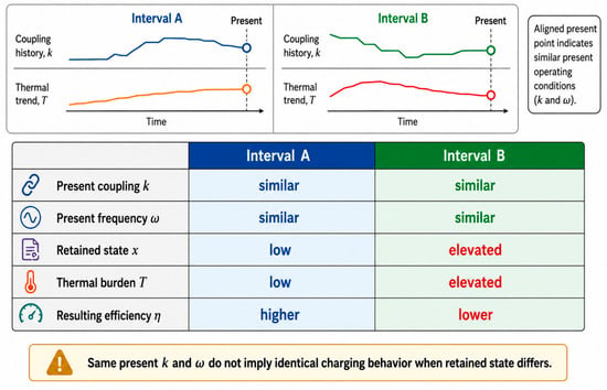
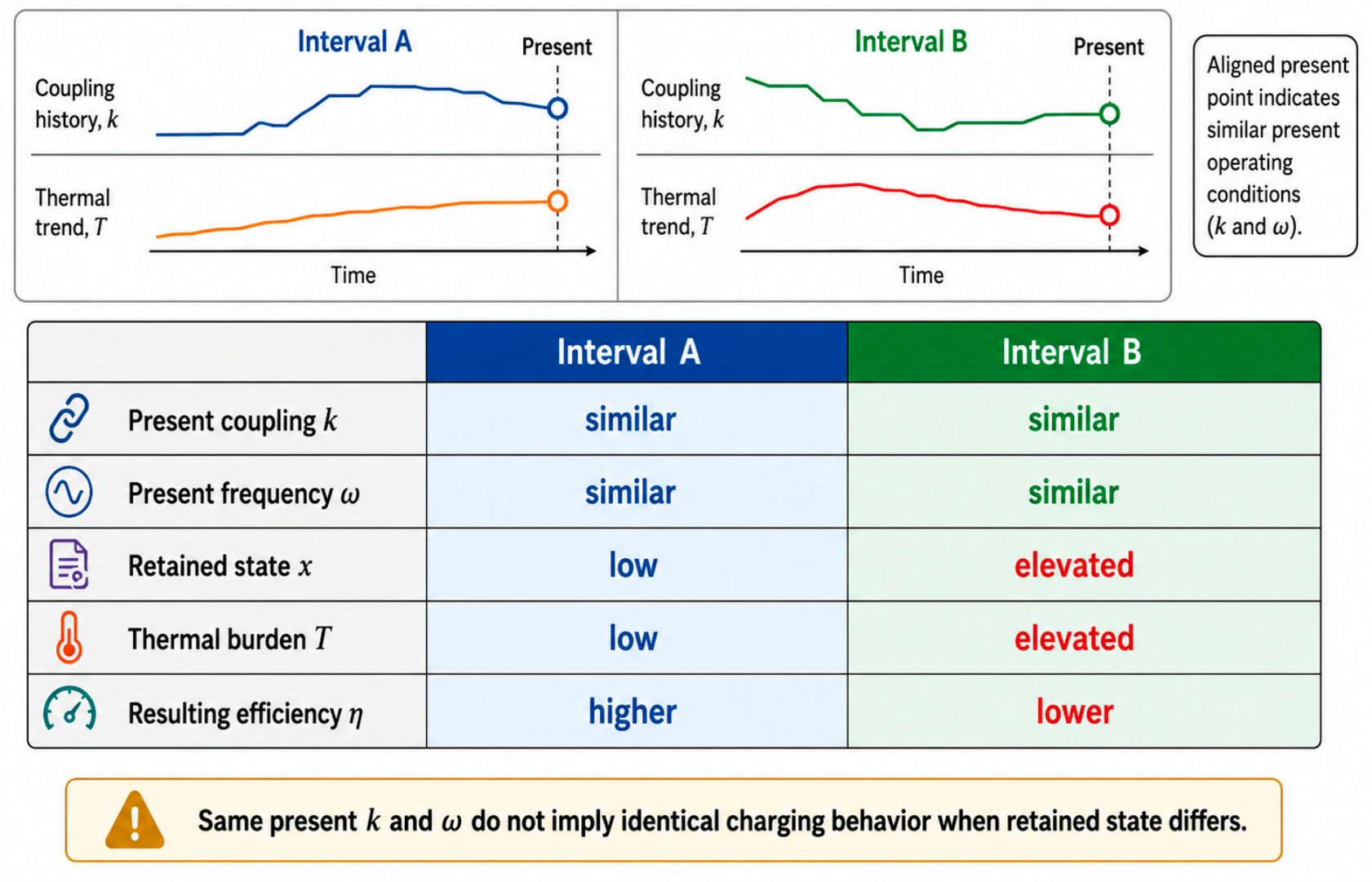
Resonant wireless EV charging provides a Layer-II test because present efficiency and current stress can depend on coupling and frequency history, retuning effort, and residual thermal burden [37,38,39,40]. The hypothesis is that two intervals with nearly identical present k and ω remain distinguishable when their retained histories differ, as illustrated in Figure 2.

Figure 2. Two charging intervals with similar present couplings and frequencies but different retained states, thermal burdens, and resulting efficiencies.

7.2.1. Reduced-Order Modeling Framework

The reduced-order model uses coupling ($k_t$), a thermal state ($T_t$), and a latent retained state ($x_t$) that aggregates prior misalignment, retuning effort, and thermal burden [40,41].

In hardware, $x_t$ could be reconstructed from coupling, frequency, current, temperature, and retuning measurements using EKF, UKF, moving-horizon, or nonlinear observer methods. The present coefficients are scenario values; calibrated implementation would require constrained nonlinear-least-squares or maximum-likelihood identification and held-out validation.

Equations (1)–(4) compare the instantaneous and retained-state efficiency formulations and define the $x_t$ evolution.

The first is a conventional instantaneous formulation:

$${\eta }_t^{\mathrm{c}\mathrm{o}\mathrm{n}\mathrm{v}}={\eta }_{\mathrm{m}\mathrm{a}\mathrm{x}}-a_1{\left(k_t-k_0\right)}^2-a_2{\left({\displaystyle \frac{{\omega }_t-{\omega }_0}{{\omega }_0}}\right)}^2-a_3\left(T_t-T_{\mathrm{a}\mathrm{m}\mathrm{b}}\right)$$

(1)

Here, $\eta$ is the charging efficiency; $k_0$ and ${\omega }_0$ are the nominal coupling coefficient and angular frequency, respectively; and $T_{\mathrm{a}\mathrm{m}\mathrm{b}}$ is the ambient temperature.

The second is a memory-aware formulation:

$${\eta }_t^{\mathrm{m}\mathrm{e}\mathrm{m}}={\eta }_{\mathrm{m}\mathrm{a}\mathrm{x}}-a_1{\left(k_t-k_0\right)}^2-a_2{\left({\displaystyle \frac{{\omega }_t-{\omega }_{t,\mathrm{e}\mathrm{f}\mathrm{f}}}{{\omega }_0}}\right)}^2-a_3\left(T_t-T_{\mathrm{a}\mathrm{m}\mathrm{b}}\right)$$

(2)

with

$${\omega }_{t,\mathrm{e}\mathrm{f}\mathrm{f}}={\omega }_0\left[1+{\gamma }_1{x}_t-{\gamma }_2\left(T_t-T_{\mathrm{a}\mathrm{m}\mathrm{b}}\right)\right]$$

(3)

and internal-state evolution,

$$x_{t+1}=\alpha x_t+{\beta }_1\left|k_t-k_{t-1}\right|+{\beta }_2{u}_t+{\beta }_3\mathrm{m}\mathrm{a}\mathrm{x} \left(0,T_t-T_{\mathrm{r}\mathrm{e}\mathrm{f}}\right)$$

(4)

Here, $u_t$ is the normalized tuning effort and $T_{\mathrm{r}\mathrm{e}\mathrm{f}}$ is the threshold above which thermal burden contributes to $x_t$.

7.2.2. Thermal and Current Submodels

The equivalent thermal state evolves according to a first-order model:

$$T_{t+1}=T_t+\mathsf{\Delta }t\left[c_1{I}_t^2-c_2\left(T_t-T_{\mathrm{a}\mathrm{m}\mathrm{b}}\right)\right]$$

(5)

where I_t is the equivalent coil current.

The current I_t is modeled by the proxy relation

$$I_t=I_0\left[1+b_1\left|k_t-k_0\right|+b_2\left|{\displaystyle \frac{{\omega }_t-{\omega }_{t,\mathrm{e}\mathrm{f}\mathrm{f}}}{{\omega }_0}}\right|\right]$$

(6)

which links current rise to both coupling deviation and detuning mismatch.

The baseline controller uses only present-coupling information:

$${\omega }_t^{\mathrm{c}\mathrm{o}\mathrm{n}\mathrm{v}}={\omega }_0-K_p\left(k_t-k_0\right)$$

(7)

whereas the memory-aware controller additionally accounts for the retained internal state:

$${\omega }_t^{\mathrm{m}\mathrm{e}\mathrm{m}}={\omega }_0-K_p\left(k_t-k_0\right)-K_x{x}_t$$

(8)

Equations (5)–(8) define thermal and current proxies and compare present-coupling retuning with retained-state-aware retuning.

7.2.3. Simulation Parameters and Scenarios

Each of the 120 synthetic sessions lasted 1800 s at 1 s resolution. Nominal operation used $f_0$ = 85 kHz; $k_0$ = 0.22; $T_{\mathrm{a}\mathrm{m}\mathrm{b}}$ = 25 °C; $T_0$ = 30 °C; $T_{\mathrm{r}\mathrm{e}\mathrm{f}}$ = 35 °C; 7 kW charging power; and ${\eta }_{\mathrm{m}\mathrm{a}\mathrm{x}}$ = 0.945. Gaussian perturbations were applied to coupling (${\sigma }_k$ = 0.002), temperature (${\sigma }_T$ = 0.15 °C), and efficiency (${\sigma }_{\eta }$ = 0.0025).

The reduced-order coefficients used in this study were: $a_1$ = 0.90; $a_2$ = 120; $a_3$ = 0.0018; $\alpha$ = 0.985; ${\beta }_1$ = 0.60; ${\beta }_2$ = 0.035; ${\beta }_3$ = 0.0025; ${\gamma }_1$ = 0.018; ${\gamma }_2$ = 0.0012; $c_1$ = 0.0025; $c_2$ = 0.010; $I_0$ = 18 A; $b_1$ = 2.5; $b_2$ = 8.0; $K_p$ = $0.035{\omega }_0$; and $K_x$ = $0.012{\omega }_0$.

Three scenarios were evaluated: stable alignment; repeated 20–40 s misalignment events every 180–240 s with k = 0.16–0.19; and dynamic parking in which geometry recovered but $x_t$ and $T_t$ remained elevated from earlier stress.

7.2.4. Evaluation Metrics

Recorded variables included the $k_t$, $T_t$, $x_t$, ${\omega }_t$, current, power, efficiency, and tuning effort. Evaluation used the efficiency RMSE, current MAE, peak temperature, settling time, and cumulative tuning effort, as well as the reactive-stress proxy in Equation (9):

$$S_{\mathrm{r}\mathrm{e}\mathrm{a}\mathrm{c}\mathrm{t}}={\sum }_t\left|{\displaystyle \frac{{\omega }_t-{\omega }_{t,\mathrm{e}\mathrm{f}\mathrm{f}}}{{\omega }_0}}\right|$$

(9)

7.2.5. Results

The Case Study I results are reported from predictive accuracy to control performance to, finally, matched-trajectory separation. Table 5 first compares the efficiency RMSEs and coil-current MAEs for the instantaneous reference, the same-information state-augmented control, and the structured memory-aware model across the three charging scenarios.

Table 5. Predictive performances of instantaneous, state-augmented, and structured memory-aware resonant-charging models.

Scenario	Model	Efficiency RMSE	Coil Current MAE (A)
Stable aligned charging	Instantaneous reference	0.0061	0.74
Stable aligned charging	State-augmented reference	0.0058	0.69
Stable aligned charging	Structured memory-aware	0.0058	0.69
Repeated partial misalignment	Instantaneous reference	0.0184	2.36
Repeated partial misalignment	State-augmented reference	0.0129	1.71
Repeated partial misalignment	Structured memory-aware	0.0129	1.71
Dynamic parking with residual thermal state	Instantaneous reference	0.0202	2.58
Dynamic parking with residual thermal state	State-augmented reference	0.0137	1.86
Dynamic parking with residual thermal state	Structured memory-aware	0.0137	1.86

To determine whether the predictive differences translate into control-relevant benefits, Table 6 compares the peak temperatures, post-disturbance settling times, cumulative tuning efforts, and reactive stresses for the instantaneous and retained-state-aware retuning laws.

Table 6. Dynamic-control comparison of instantaneous and structured memory-aware retuning in resonant wireless charging.

Scenario	Controller	Peak Temp (°C)	Settling Time (s)	Tuning Effort	Reactive Stress Proxy
Stable aligned charging	Instantaneous reference	42.3	7.8	0.118	5.42
Stable aligned charging	Structured memory-aware	41.9	7.1	0.109	5.03
Repeated partial misalignment	Instantaneous reference	58.7	24.6	0.461	16.80
Repeated partial misalignment	Structured memory-aware	54.1	18.9	0.389	13.76
Dynamic parking with residual thermal state	Instantaneous reference	61.3	27.2	0.497	18.22
Dynamic parking with residual thermal state	Structured memory-aware	56.0	20.8	0.414	14.91

Beyond the aggregate error and stress measures, the trajectory-dependence hypothesis is examined at two nearly coincident operating points. Table 7 contrasts a representative pair with similar present couplings and frequencies but markedly different retained states.

Table 7. Representative operating intervals with nearly identical present couplings and operating frequencies but different retained trajectory states.

Interval	k	$\mathit{\omega }/{\mathit{\omega }}_0$	Temp (°C)	x	η
A	0.219	1.003	43.0	0.08	0.919
B	0.220	1.003	43.6	0.31	0.903

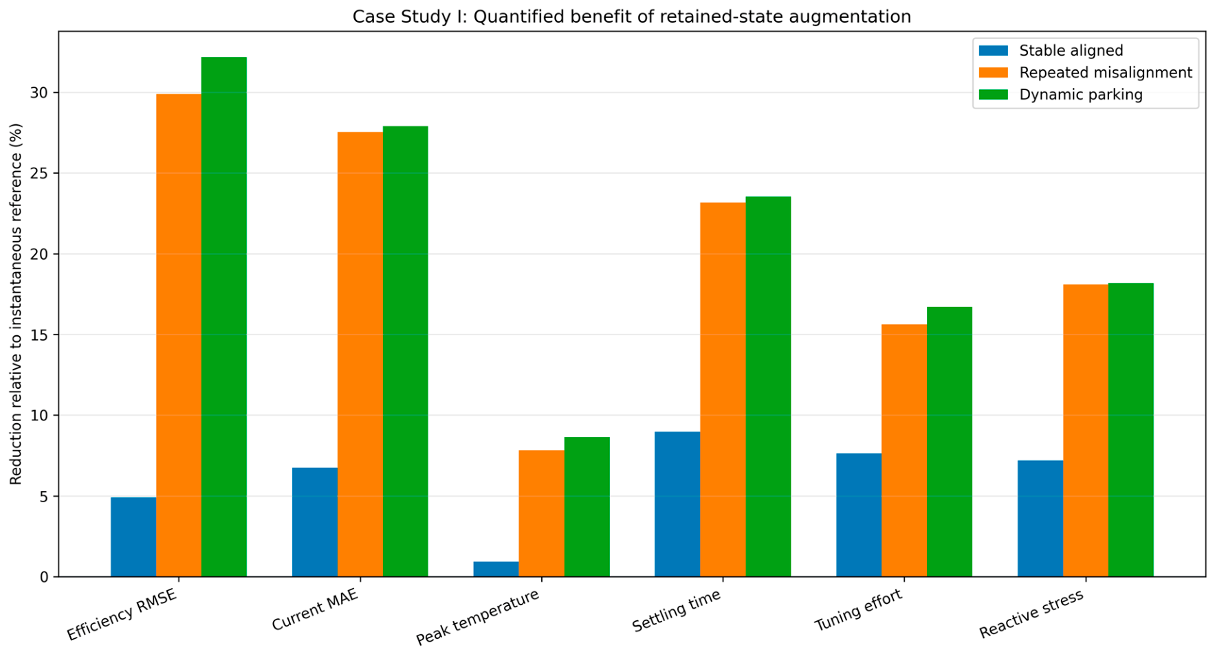
Table 5 confirms the purpose of the same-information control: the state-augmented and structured memory-aware rows are numerically identical, while both differ from the instantaneous reference. Under stable alignment, retained-state augmentation reduced the efficiency RMSE by 4.9% and the current MAE by 6.8%. Under repeated misalignment, the reductions were 29.9% and 27.5%; under dynamic parking, they were 32.2% and 27.9%, respectively.

The control-oriented gains were also concentrated in the disturbed trajectories. Repeated misalignment produced reductions of 7.8% in peak temperature, 23.2% in settling time, 15.6% in tuning effort, and 18.1% in reactive stress. Dynamic parking produced corresponding reductions of 8.6%, 23.5%, 16.7%, and 18.2%. For the representative intervals in Table 7, the efficiency difference was 0.016, equivalent to a normalized separation ($M_{\mathrm{T}\mathrm{S}}$) of 0.0088 and a noise-normalized separation ($M_{\mathrm{N}\mathrm{S}}$) of 6.4 relative to the declared efficiency noise (${\sigma }_{\eta }$ ta = 0.0025). Thus, the separation is small in absolute efficiency units but well above the simulated observation-noise scale.

Figure 3 condenses these scenario-level results into percentage reductions relative to the instantaneous reference, making clear that the largest gains occur under repeated disturbance and residual thermal burden.

Figure 3. Relative reductions versus instantaneous reference in Case Study I; state-augmented and structured models are numerically identical.

7.2.6. Trajectory Bifurcation Test

Paths A and B converge to nearly identical k and ω but retain different $x_t$; the resulting efficiency and current-stress difference confirms trajectory dependence:

$$k_A\left(t_f\right)\approx k_B\left(t_f\right), {\omega }_A\left(t_f\right)\approx {\omega }_B\left(t_f\right)$$

$$x_A\left(t_f\right)\ne x_B\left(t_f\right)$$

7.3. Case Study II: History-Aware Battery Charging and V2G Scheduling

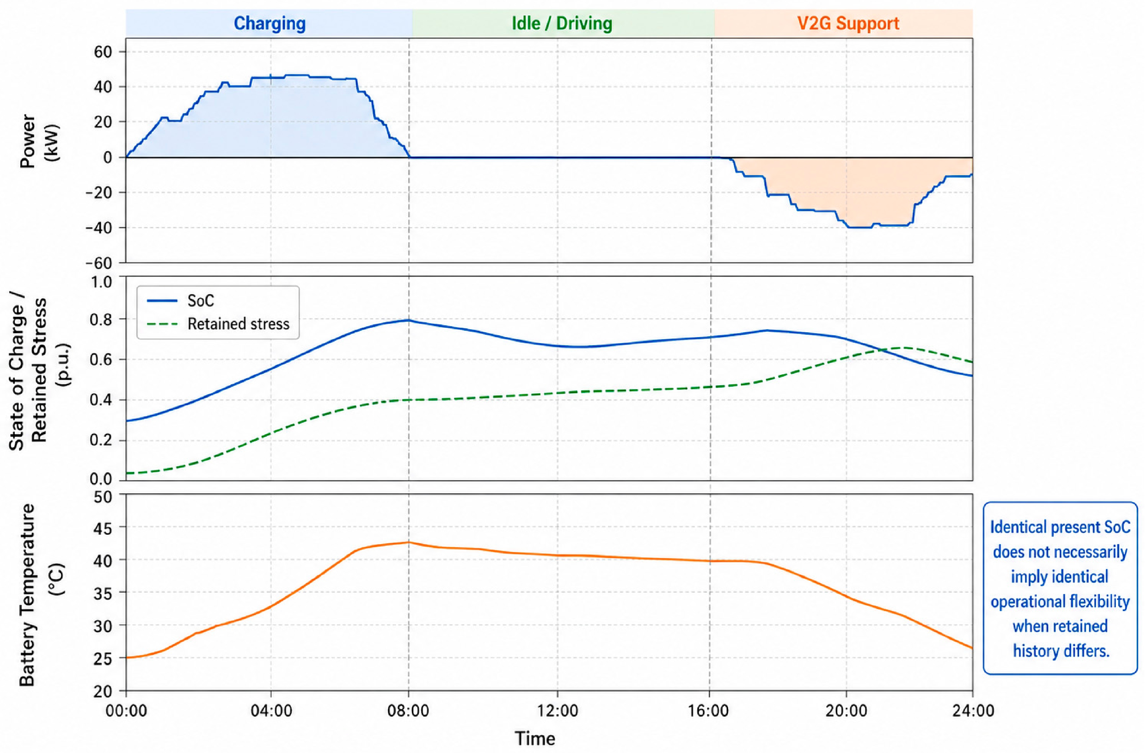
Case Study II tests Layer III: whether identical present SoCs imply identical V2G flexibilities when degradation, thermal exposure, and recent dispatch stress differ. Figure 4 illustrates the daily evolution of the power, SoC, retained stress, and temperature.

Figure 4. Representative daily history-aware EV charging/V2G cycle showing power, SoC, retained stress, and temperature.

7.3.1. Fleet Model and Time Horizon

A heterogeneous fleet of 20 EVs was simulated over 24 h at 15 min resolution with time-varying tariffs, feeder constraints, and an 18:00–21:00 V2G window. Each EV had 60 kWh capacity, 7 kW charging, 5 kW discharging, ${\eta }_c$ = 0.95, ${\eta }_d$ = 0.94, ${\mathrm{S}\mathrm{o}\mathrm{C}}_{\mathrm{m}\mathrm{i}\mathrm{n}}$ = 20%, and a 50–80% departure target; four five-vehicle mobility groups introduced usage heterogeneity.

7.3.2. State Equations

For each vehicle (i), the state of charge evolves according to:

$${\mathrm{S}\mathrm{o}\mathrm{C}}_i\left(t+1\right)={\mathrm{S}\mathrm{o}\mathrm{C}}_i\left(t\right)+{\displaystyle \frac{{\eta }_c{P}_{c,i}\left(t\right)-P_{d,i}\left(t\right)/{\eta }_d}{E_i}}\hspace{0.17em}\mathsf{\Delta }t$$

(10)

where $P_{c,i}\left(t\right)$ and $P_{d,i}\left(t\right)$ denote the charging and discharging power, respectively.

The battery thermal state evolves according to a reduced-order proxy model:

$$T_i\left(t+1\right)=T_i\left(t\right)+\mathsf{\Delta }t\left\{{\mu }_1{\left[P_{c,i}\left(t\right)+P_{d,i}\left(t\right)\right]}^2-{\mu }_2\left[T_i\left(t\right)-T_{\mathrm{a}\mathrm{m}\mathrm{b}}\left(t\right)\right]\right\}$$

(11)

with ${\mu }_1$ = 0.010 and ${\mu }_2$ = 0.065.

To capture retained usage history, a degradation-memory state ($D_i\left(t\right)$) was introduced:

$$D_i\left(t+1\right)=\rho D_i\left(t\right)+{\nu }_1\left|P_i\left(t\right)\right|+{\nu }_2\mathrm{m}\mathrm{a}\mathrm{x} \left(0,T_i\left(t\right)-T_{\mathrm{t}\mathrm{h}}\right)+{\nu }_3{\delta }_{\mathrm{H}\mathrm{L},i}\left(t\right)$$

(12)

with $\rho$ = 0.96, ${\nu }_1$ = 0.018, ${\nu }_2$ = 0.022, and ${\nu }_3$ = 0.25.

A second internal state ($H_i\left(t\right)$) was used to represent recent charging/discharging stress:

$$H_i\left(t+1\right)=\lambda H_i\left(t\right)+\left(1-\lambda \right)\left|P_i\left(t\right)-P_i\left(t-1\right)\right|$$

(13)

with $\lambda$ = 0.85.

Here, $P_i\left(t\right)=P_{c,i}\left(t\right)-P_{d,i}\left(t\right)$ is the signed battery power, $T_{\mathrm{t}\mathrm{h}}={35 }^{\circ }\mathrm{C}$, and ${\delta }_{\mathrm{H}\mathrm{L},i}\left(t\right)\in \{0,1\}$ identifies a fast/high-load event. $D_i$(t) and $H_i$(t) are the reduced-order latent states for the cumulative degradation burden and recent charge/discharge stress; they are not substitutes for electrochemical aging models.

7.3.3. Baseline and History-Aware Scheduling

The first is a baseline SoC-based scheduler, which uses only current SoC, mobility requirements, price signals, and feeder-load penalties. Its objective is:

$$J_{\mathrm{b}\mathrm{a}\mathrm{s}\mathrm{e}}=\mathsf{\Delta }t{\sum }_t\left[c\left(t\right)P_{\mathrm{g}\mathrm{r}\mathrm{i}\mathrm{d}}\left(t\right)+\kappa \mathrm{m}\mathrm{a}\mathrm{x} \left(0,L\left(t\right)-L^{\mathrm{*}}\right)\right]$$

(14)

where c(t) is the time-varying electricity tariff, L(t) is the feeder load, L* is the desired peak threshold, and κ = 0.18.

The second is a history-aware scheduler, which augments the above objective by including accumulated stress penalties:

$$J_{\mathrm{h}\mathrm{i}\mathrm{s}\mathrm{t}}=J_{\mathrm{b}\mathrm{a}\mathrm{s}\mathrm{e}}+\mathsf{\Delta }t{\sum }_{i,t}\left[\alpha D_i\left(t\right)+\beta H_i\left(t\right)+\gamma \mathrm{m}\mathrm{a}\mathrm{x} \left(0,T_i\left(t\right)-T_{\mathrm{t}\mathrm{h}}\right)\right]$$

(15)

with $\alpha$ = 0.06, $\beta$ = 0.025, and $\gamma$ = 0.04.

The objective is expressed in EUR/day. With the common factor (Δt) included in Equations (14) and (15), $\kappa$ has units EUR/(kW·h), $\alpha$ and $\beta$ have units EUR/(normalized-state-unit·h), and $\gamma$ has units EUR/(°C·h). These scenario weights require recalibration for another fleet.

7.3.4. Inputs, Scenarios, and Metrics

The initial SoC was 35–80%, the temperature was 24–32 °C, and the trip demand was 6–28 kWh/day by vehicle group; the ambient temperature varied from 21 to 32 °C. The tariff is listed below, and up to 28 kW aggregated V2G support was requested from 18:00 to 21:00.

The time-varying electricity tariff was defined as follows:

Time Interval	Price (EUR/kWh)
00:00–06:00	0.16
06:00–12:00	0.22
12:00–16:00	0.18
16:00–21:00	0.31
21:00–24:00	0.20

Three scenarios were tested: equal SoCs with different histories; peak support after heavy daytime use; and midday surplus followed by evening V2G.

Recorded states and decisions included availability, SoC, temperature, $D_i$, $H_i$, charge/discharge power, mobility demand, and V2G participation. Metrics were cost, peak reduction, V2G revenue, unmet departure events, degradation proxy, thermal violations, and the aggressive-cycling index in Equation (16).

The aggressive-cycling index was defined as:

$$C_{\mathrm{a}\mathrm{g}\mathrm{g}}={\sum }_{i,t}\left|P_i\left(t\right)-P_i\left(t-1\right)\right|$$

(16)

7.3.5. Results

The Case Study II results are organized from fleet-level outcomes to individual dispatch separation and scenario robustness. Table 8 first compares the SoC-only baseline with the same-information state-augmented and structured memory-aware schedules across economic, grid-support, degradation, thermal, and cycling metrics.

Table 8. Fleet-level comparison of SoC-only, state-augmented, and structured memory-aware charging/V2G scheduling.

Metric	SoC-Only Baseline	State-Augmented Reference	Structured Memory-Aware
Total charging cost (EUR/day)	79.4	76.8	76.8
Peak feeder-load reduction (%)	17.9	15.8	15.8
V2G revenue (EUR/day)	11.6	10.8	10.8
Unmet departure-SoC events	0	0	0
Cumulative degradation proxy	148.2	130.4	130.4
Thermal-limit violations	11	8	8
Aggressive-cycling index	412.5	341.7	341.7

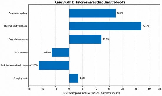
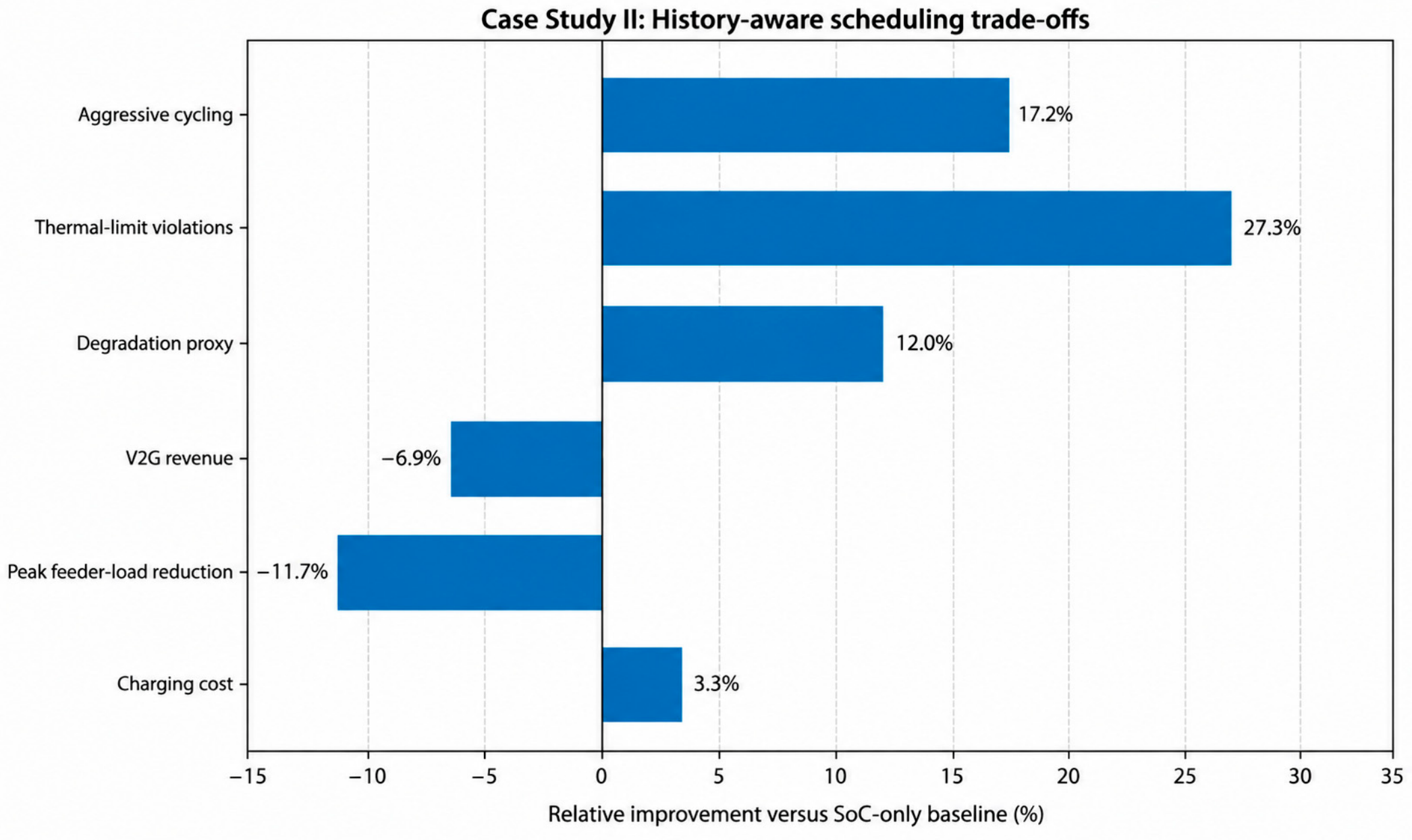
The same-information control again yielded identical state-augmented and structured results. Relative to the SoC-only baseline, the state-aware schedule reduced the charging cost by 3.3%, the cumulative degradation proxy by 12.0%, thermal-limit violations by 27.3%, and aggressive cycling by 17.2% while preserving all departure-SoC requirements. These benefits were obtained at the cost of an 11.7% reduction in the peak feeder-load reduction and a 6.9% reduction in V2G revenue, demonstrating a genuine multi-objective trade-off rather than universal superiority.

To expose the direction and magnitude of this multi-objective trade-off, Figure 5 expresses each state-aware outcome as a relative change from the SoC-only baseline.

Figure 5. Relative changes produced by state-aware scheduling in Case Study II; negative values identify sacrifices in peak reduction and V2G revenue.

Aggregate fleet metrics do not by themselves show how retained history changes individual dispatch decisions. Table 9 therefore compares two vehicles with identical present SoCs but different degradation, thermal, and recent-stress states.

Table 9. Representative comparison of two EVs with identical present SoCs but different retained histories at 18:00.

EV	SoC	Temp (°C)	Degradation State (D)	Stress State (H)	Baseline V2G Dispatch (kW)	Structured Memory-Aware V2G Dispatch (kW)
EV-07	0.60	33.8	2.41	1.92	3.0	1.2
EV-14	0.60	31.2	1.08	0.84	2.8	3.6

Table 9 illustrates the decision-level trajectory separation. Under the SoC-only baseline, the two vehicles receive nearly identical V2G assignments (3.0 and 2.8 kW; difference: 0.2 kW). Under the structured state-aware schedule, their assignments diverge to 1.2 and 3.6 kW (difference: 2.4 kW), a twelve-fold increase in decision separation that reflects the different degradation, thermal, and recent-stress histories rather than present SoCs.

To test whether this decision logic persists under different operating demands, Table 10 reports the baseline and structured memory-aware results for the three fleet scenarios.

Table 10. Scenario-level comparison of baseline and history-aware scheduling.

Scenario	Controller	Cost (EUR)	Peak Reduction (%)	Degradation Proxy	Thermal Violations
Same SoCs/different histories	Baseline	77.1	12.6	136.2	6
Same SoCs/different histories	Structured memory-aware	76.4	11.8	121.7	4
Peak support under stressed fleet	Baseline	81.5	18.9	154.6	12
Peak support under stressed fleet	Structured memory-aware	79.8	16.7	134.5	8
Midday surplus + evening V2G	Baseline	79.7	18.1	153.8	10
Midday surplus + evening V2G	Structured memory-aware	77.9	16.3	135.1	7

Across scenarios, history-aware scheduling consistently reduced retained burden and thermal violations while preserving mobility but did not maximize every grid-service objective.

7.4. Case Study III: Public-Experimental-Data Validation of Layer-I Retained-State Relevance

7.4.1. Dataset and Validation Protocol

The public NASA Ames Prognostics Center of Excellence (PCoE) Li-ion Battery Aging Dataset was used to add a bounded experimental-data study at Layer I. The dataset was collected on a custom battery prognostics testbed using commercial 18650 cells and includes charge, discharge, and impedance operations with measured terminal voltage, current, temperature, time, and discharge capacity [47,48]. The present analysis used 636 discharge cycles from cells B0005, B0006, B0007, and B0018.

For each cycle, the operating point nearest 3.75 V was extracted. The instantaneous descriptor contained the terminal voltage, current, temperature, local voltage slope, local temperature slope, and discharged ampere-hours within the current cycle. The retained-history descriptor contained cumulative prior discharge throughput and previous-cycle capacity. Candidate pairs were formed within each cell only when they were separated by at least 40 cycles and satisfied the predeclared matching limits |ΔV| ≤ 3 mV, |ΔI| ≤ 10 mA, |ΔT| ≤ 0.75 °C, |Δ(dV/dt)| ≤ 80 μV/s, and |Δ(dT/dt)| ≤ 0.003 °C/s. Candidates were ranked by normalized instantaneous-state distance and selected deterministically without reusing a cycle.

The output used for trajectory testing was the 900 s voltage evolution following the matched point, sampled every 30 s. $M_{\mathrm{T}\mathrm{S}}$ was evaluated from the future voltage-drop vectors, while $M_{\mathrm{N}\mathrm{S}}$ used a conservative 1 mV per-sample reference scale. Retained-state relevance was assessed by leave-one-battery-out cross-validation. The instantaneous model used only the current-cycle descriptor; the history-augmented model added cumulative prior throughput and previous capacity. Identical model classes were used on both feature sets. A random forest was predeclared as the primary nonlinear test and ridge regression was retained as a model-class sensitivity check. The complete extraction, pairing, bootstrap, and prediction workflow is provided in Supplementary File S1.

7.4.2. Experimental Results

The experimental evidence is summarized at aggregate level before the individual trajectory example is examined. Table 11 reports the matched-pair quality, future-trajectory separation, statistical significance, and leave-one-battery-out retained-state relevance obtained from the NASA data.

Table 11. Public-experimental-data validation of Layer-I retained-state relevance using NASA Ames PCoE battery-aging dataset.

Validation Quantity	Result	Interpretation
Experimental coverage	4 cells; 636 discharge cycles	NASA public Layer-I data
Matched-pair sample	120 cycle–disjoint pairs; median gap: 42 cycles	Within-cell lifecycle-history contrast
Median instantaneous mismatch	0.54 mV; 1.56 mA; 0.20 °C	Local voltage and temperature slopes also matched
Remaining-discharge-time separation	150.7 s (95% bootstrap CI: 137.8–159.7 s)	All later-history cycles had shorter remaining duration; p < 10−21
Capacity separation	0.133 Ah (95% CI: 0.117–0.142 Ah)	All later-history cycles had lower capacity; p < 10−21
Trajectory-separation index	$\mathrm{Median} M_{\mathrm{T}\mathrm{S}}$ = 0.0688 (95% CI: 0.0645–0.0740)	Future trajectories remain distinguishable after state matching
Noise-normalized separation	$\mathrm{Median} M_{\mathrm{N}\mathrm{S}}$ = 20.13 (95% CI: 18.61–22.49)	Separation exceeds the conservative 1 mV reference scale
Random-forest LOBO prediction	$\mathrm{MAE} 113.2 \to 95.2 \mathrm{s}; M_{\mathrm{R}\mathrm{I}}$ = 0.159 (95% CI: 0.121–0.194)	Positive out-of-battery retained-state relevance
Ridge sensitivity check	$\mathrm{MAE} 191.1 \to 81.2 \mathrm{s}; M_{\mathrm{R}\mathrm{I}}$ = 0.575	Positive relevance is not restricted to one model class

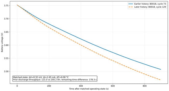
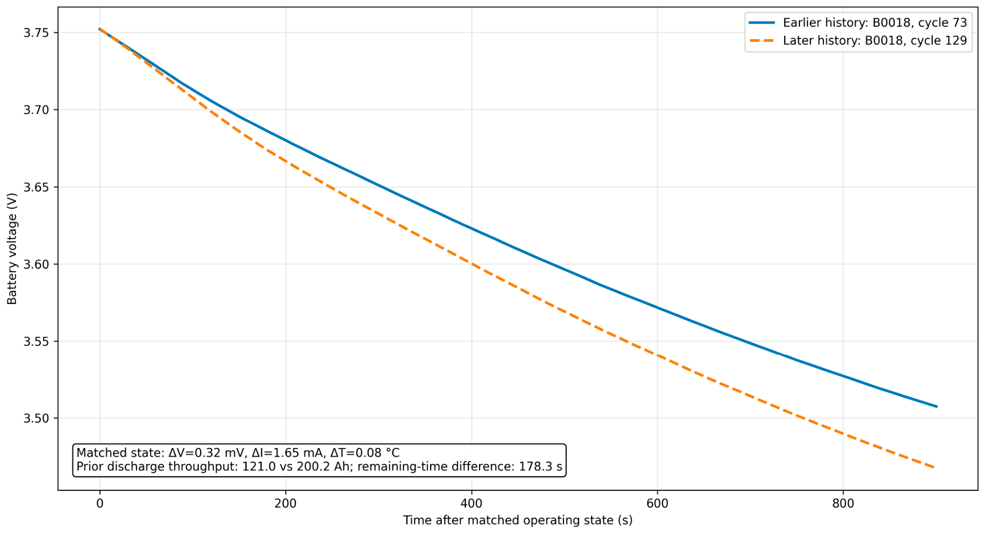
The matching procedure produced 120 cycle–disjoint pairs across all four cells. Their median state mismatch was only 0.54 mV, 1.56 mA, and 0.20 °C, yet the median remaining-discharge-time separation was 150.7 s and the median capacity separation was 0.133 Ah. Every later-history cycle in the matched sample had a lower remaining duration and lower measured capacity than its earlier-history counterpart (one-sided paired Wilcoxon tests, p < 10⁻²¹). The median $M_{\mathrm{T}\mathrm{S}}$ was 0.0688 and the median $M_{\mathrm{N}\mathrm{S}}$ was 20.13, satisfying the trajectory-separation and uncertainty criteria of Section 2.1.

The out-of-battery prediction test was deliberately stricter than random cycle splitting. With one entire cell held out at a time, the primary random-forest model reduced the MAE from 113.2 to 95.2 s after the retained-history variables were added, giving $M_{\mathrm{R}\mathrm{I}}$ = 0.159 (95% bootstrap interval: 0.121–0.194; paired-error p = 1.23 × 10⁻¹³). Ridge regression produced the same direction of effect, reducing the MAE from 191.1 to 81.2 s and giving $M_{\mathrm{R}\mathrm{I}}$ = 0.575. A conventional state-augmented model and the structured Layer-I interpretation use the same numerical variables and therefore have identical prediction results; the added contribution of the framework is the admissibility, physical interpretation, matching, and falsification logic applied to those variables.

To illustrate the physical meaning of these aggregate statistics, Figure 6 shows one matched B0018 pair that is nearly indistinguishable at the selected operating point but diverges over the subsequent discharge trajectory.

Figure 6. A representative NASA B0018 pair from the cycle–disjoint matched sample. Cycles 73 and 129 reach nearly identical voltages, currents, temperatures, and local slopes at the matched point, but their subsequent 900 s voltage trajectories diverge after different prior discharge throughput (121.0 versus 200.2 Ah). The later-history cycle has 178.3 s less remaining-discharge duration.

This study provides partial public-experimental-data validation of Layer I. After conditioning on closely matched present electrical and thermal states, retained lifecycle history remains associated with distinguishable future voltage behavior and remaining-discharge capability. The result does not establish that the complete cell is a strict memcapacitive element or validate a universal electrochemical constitutive law. It supports the narrower claim that electrochemical degradation and prior throughput form physically grounded retained states with measurable engineering consequences.

7.5. Cross-Case Interpretation

The three applications now span the proposed hierarchy. The NASA study provides public-experimental-data support for Layer I by showing that closely matched present electrical and thermal states can retain different lifecycle consequences. Case Study I demonstrates the same structural logic at Layer II through resonant-converter trajectories, and Case Study II demonstrates it at Layer III through charging/V2G decisions. Across all layers, similar present variables can conceal distinct histories that alter voltage evolution, remaining capability, efficiency, stress, degradation, or dispatch. The combined evidence supports a bounded retained-state interpretation, not universal constitutive equivalence or deployment-ready superiority.

7.6. Parameter Sensitivity and Robustness Analysis

One-at-a-time perturbations examined whether the Layer-II and Layer-III trajectory distinctions persisted when the reduced-order coefficients were varied over the ranges in Table 12 and Table 13.

Table 12. Sensitivity ranges and retained qualitative outcomes for Case Study I.

Retained Qualitative Outcome	Tested Range	Nominal Values	Parameter Group
Scenario ordering and disturbed-trajectory separation preserved	±20%	0.90; 120; 0.0018	$\mathrm{Efficiency} \mathrm{penalties}, a_1–a_3$
Misalignment, tuning-effort, and residual-thermal effects remain visible	$\alpha :0.970–0.995;$ $\hspace{0.25em}{\beta }_1:0.45–0.75;$ $\hspace{0.25em}{\beta }_2:0.020–0.050;$ $\hspace{0.25em}{\beta }_3:0.0015–0.0040$	0.985; 0.60; 0.035; 0.0025	$\mathrm{Memory} \mathrm{evolution}, \alpha$$, {\beta }_1–{\beta }_3$
Magnitude changes, but efficiency-separation direction is preserved	±30%	0.018; 0.0012	$\mathrm{Frequency} \mathrm{corrections}, {\gamma }_1,\hspace{0.25em}{\gamma }_2$
Current-stress and thermal scenario rankings remain preserved	±20%	2.5; 8.0; 0.0025; 0.010	$\mathrm{Current}/\mathrm{thermal} \mathrm{terms}, b_1,\hspace{0.25em}{b}_2,\hspace{0.25em}{c}_1,\hspace{0.25em}{c}_2$
Settling-time trend and retained-state-aware benefit remain preserved	$K_p:\left(0.025–0.045\right){\omega }_0;$ $K_x:\left(0.006–0.018\right){\omega }_0$	$0.035{\omega }_0$$; 0.012{\omega }_0$	$\mathrm{Retuning} \mathrm{gains}, K_p,\hspace{0.25em}{K}_x$

Table 13. Sensitivity ranges and retained qualitative outcomes for Case Study II.

Retained Qualitative Outcome	Tested Range	Nominal Values	Parameter Group
Relative thermal-burden distinction remains preserved	±20%	0.010; 0.065	$\mathrm{Thermal} \mathrm{terms}, {\mu }_1,\hspace{0.25em}{\mu }_2$
Stressed and high-utilization vehicles remain more constrained; direction preserved	$\rho :0.90–0.99;\hspace{0.25em}{\nu }_1–{\nu }_3:\pm 30\%$	0.96; 0.018; 0.022; 0.25	$\mathrm{Degradation} \mathrm{memory}, \rho$$, {\nu }_1–{\nu }_3$
Recent-stress separation remains visible	0.75–0.95	0.85	Stress persistence, λ
Peak-reduction trade-off changes, but mobility constraints remain satisfied	±25%	0.18	Feeder penalty, κ
Lower degradation, cycling, and thermal-violation trends remain preserved	±30%	0.06; 0.025; 0.04	History weights, α, β, γ

7.6.1. Case Study I

Case Study I varied the efficiency, state-evolution, frequency-correction, thermal/current, and retuning parameters.

The robustness analysis for Case Study I is organized by parameter group in Table 12, which links each tested range to the qualitative outcome retained under perturbation.

Although absolute errors and stresses changed, stable alignment retained small differences, whereas disturbed trajectories remained separated; the direction of the main result was preserved.

7.6.2. Case Study II

Case Study II varied the thermal, degradation-memory, stress-persistence, and scheduling weights.

Table 13 applies the same structure to Case Study II and identifies which thermal, degradation-memory, stress-persistence, and scheduling-weight perturbations preserve the history-dependent dispatch pattern.

Cost and grid-service trade-offs changed quantitatively, but vehicles with equal SoCs and different histories remained operationally distinguishable, and the history-aware solution continued to reduce burden and cycling in the tested ranges.

Together, the sensitivity tests show that the qualitative retained-state effect is not an artifact of a single parameter set while confirming that its magnitude and preferred trade-off remain application-dependent.

8. Discussion, Limitations, and Implementation Challenges

The proposed contribution is a bounded classification-and-testing framework, not a replacement for state-space modeling, model predictive control, reinforcement learning, digital twins, electrochemical models, or established converter analysis. The same-information controls show explicitly that the structured framework does not create a numerical advantage over conventional state augmentation. Its novelty lies instead in deciding when a retained variable is admissible, assigning it to a defensible layer, quantifying its relevance, requiring observability, and rejecting the memory-aware label when these conditions are not met.

Deployment requires the observer-based reconstruction of latent states from electrical, thermal, magnetic, and operational measurements, followed by constrained nonlinear-least-squares, maximum-likelihood, or Bayesian calibration and held-out validation. Comparisons must retain the instantaneous, same-information state-augmented, and structured formulations so that benefit is not attributed merely to additional inputs.

Practical implementation adds hardware variability, sensing, storage, communication, estimation, cybersecurity, and computational overhead. The NASA analysis provides partial public-experimental-data validation of Layer I, whereas the Layer-II and Layer-III studies remain reduced-order proof-of-concept demonstrations. The combined evidence supports the claim that retained-state augmentation can reveal trajectory dependence hidden by instantaneous formulations; it does not establish universal superiority, industrial readiness, or constitutive equivalence across layers.

9. Research and Validation Roadmap

The completed NASA study establishes the first public-experimental-data checkpoint for Layer I, but the framework should continue through staged validation rather than broad conceptual expansion. Each subsequent stage must use the same acceptance logic: retained states must be identifiable, produce trajectory separation above uncertainty, provide positive out-of-sample relevance, and deliver an engineering benefit that exceeds sensing, estimation, communication, and computational overhead.

The resulting validation priorities are consolidated in Table 14 as a staged roadmap with explicit evidence requirements and exit criteria for each development horizon.

Table 14. Staged research and validation roadmap for proposed three-layer framework.

Horizon	Primary Objective	Required Evidence and Methods	Exit Criteria
Near term (0–2 years)	Extend the completed NASA Layer-I study to additional chemistries and identify retained states in converters, charging interfaces, and digital twins	Additional hardware/public datasets; observer design; constrained system identification; instantaneous and same-information state-augmented baselines	$M_{\mathrm{T}\mathrm{S}}$$\mathrm{above} \mathrm{uncertainty}, \mathrm{positive} M_{\mathrm{R}\mathrm{I}}$, bounded estimation error, and reproducible parameter identification
Mid-term (2–5 years)	Integrate retained-state models with MPC, diagnostics, HIL platforms, and fleet/grid pilots	Cross-site validation; estimator and controller robustness; cyber-physical overhead accounting; multi-objective benchmark studies	Engineering gains remain significant after overhead, uncertainty, and baseline-equivalence tests
Long term (5+ years)	Co-design physical mem-elements, converter memory, and adaptive energy architectures	Device reliability and lifetime data; multi-layer observability; lifecycle, safety, cybersecurity, and interoperability assessment	Deployment readiness without conflating constitutive, mem-inspired, and functional memory claims

Cross-layer progress is necessary but not automatically cumulative. Device-level advances must be linked to converter-level consequences, and higher-level operational memory must remain traceable to measurable states or defensible functional records. A stage should not proceed when the same engineering conclusion is obtained with a simpler conventional model.

10. Conclusions

This study developed a falsifiable three-layer framework that distinguishes constitutive physical memory, distributed circuit/converter memory, and functional operational memory. Inclusion, trajectory-separation, relevance, engineering-gain, observability, and rejection tests determine whether an added state has memory-specific engineering meaning; same-information controls confirm that the framework does not claim numerical superiority over conventional state augmentation.

The public NASA validation supplied the previously missing Layer-I evidence. Across 120 closely matched experimental cycle pairs, the median remaining-discharge-time difference was 150.7 s, the $M_{\mathrm{T}\mathrm{S}}$ was 0.0688, and the $M_{\mathrm{N}\mathrm{S}}$ was 20.13, and leave-one-battery-out prediction yielded positive retained-state relevance. In the resonant-charging Layer-II case, retained-state augmentation reduced the efficiency RMSE by 29.9–32.2% and the current MAE by 27.5–27.9% in the disturbed scenarios while reducing the settling time by approximately 23% and reactive stress by approximately 18%. In the EV/V2G Layer-III case, state-aware scheduling reduced the charging cost by 3.3%, the degradation proxy by 12.0%, thermal violations by 27.3%, and aggressive cycling by 17.2% while sacrificing 11.7% of peak-reduction performance and 6.9% of V2G revenue.

The evidence is intentionally asymmetric: Layer I now has bounded public-experimental-data validation, whereas Layers II and III remain proof-of-concept applications. The decisive next steps are independent hardware replication, observer-based state reconstruction, additional chemistries and converter platforms, and same-information benchmark studies under deployment conditions. Mem-element theory is most defensible when physically literal and experimentally testable at Layer I, mem-inspired and quantitatively testable at Layer II, and explicitly functional at Layer III.

References

- Dimitriadou, K.; Rigogiannis, N.; Fountoukidis, S.; Kotarela, F.; Kyritsis, A.; Papanikolaou, N. Current trends in electric vehicle charging infrastructure: Opportunities and challenges in wireless charging integration. Energies 2023, 16, 2057. [Google Scholar] [CrossRef] [Scilit]
- Ahmad, A.; Khalid, M.; Ullah, Z.; Ahmad, N.; Aljaidi, M.; Malik, F.A.; Manzoor, U. Electric vehicle charging modes, technologies and applications of smart charging. Energies 2022, 15, 9471. [Google Scholar] [CrossRef] [Scilit]
- Chua, L. Memristor—The missing circuit element. IEEE Trans. Circuit Theory 1971, 18, 507–519. [Google Scholar] [CrossRef] [Scilit]
- Strukov, D.; Snider, G.; Stewart, D.; Williams, R.S. The missing memristor found. Nature 2008, 453, 80–83. [Google Scholar] [CrossRef] [Scilit] [PubMed]
- Kundu, S.; Dutta, R. Memristor: The missing fourth circuit component. In Low-Dimensional Nanoelectronic Devices; Apple Academic Press: Waretown, NJ, USA, 2022; pp. 243–261. [Google Scholar]
- Sun, Y. The fourth fundamental circuit element: Principle and applications. J. Phys. D Appl. Phys. 2022, 55, 253001. [Google Scholar] [CrossRef] [Scilit]
- Vaidyanathan, S.; Volos, C. (Eds.) Advances in Memristors, Memristive Devices and Systems; Springer: Berlin, Germany, 2017; Volume 701. [Google Scholar]
- Isah, A.; Bilbault, J.-M. Review on the basic circuit elements and memristor interpretation: Analysis, technology and applications. J. Low Power Electron. Appl. 2022, 12, 44. [Google Scholar] [CrossRef] [Scilit]
- Yin, Z.; Tian, H.; Chen, G.; Chua, L.O. What are memristor, memcapacitor, and meminductor? IEEE Trans. Circuits Syst. II Express Briefs 2015, 62, 402–406. [Google Scholar] [CrossRef] [Scilit]
- Tellini, B.; Bologna, M.; Chandía, K.J.; Macucci, M. Revisiting the memristor concept within basic circuit theory. Int. J. Circuit Theory Appl. 2021, 49, 3488–3506. [Google Scholar] [CrossRef] [Scilit]
- Corinto, F.; Forti, M. Memristor circuits: Flux–charge analysis method. IEEE Trans. Circuits Syst. I Regul. Pap. 2016, 63, 1997–2009. [Google Scholar] [CrossRef] [Scilit]
- Song, M.K.; Kang, J.H.; Zhang, X.; Ji, W.; Ascoli, A.; Messaris, I.; Demirkol, A.S.; Dong, B.; Aggarwal, S.; Wan, W.; et al. Recent advances and future prospects for memristive materials, devices, and systems. ACS Nano 2023, 17, 11994–12039. [Google Scholar] [CrossRef] [Scilit] [PubMed]
- Vasileska, D.; Goodnick, S.M. Computational Electronics; Springer Nature: Cham, Switzerland, 2022. [Google Scholar]
- Lyshevski, S.E. (Ed.) Nano and Molecular Electronics Handbook; CRC Press: Boca Raton, FL, USA, 2018. [Google Scholar]
- Di Ventra, M.; Pershin, Y.V.; Chua, L.O. Circuit elements with memory: Memristors, memcapacitors, and meminductors. Proc. IEEE 2009, 97, 1717–1724. [Google Scholar] [CrossRef] [Scilit]
- Zidan, M.A.; Strachan, J.P.; Lu, W.D. The future of electronics based on memristive systems. Nat. Electron. 2018, 1, 22–29. [Google Scholar] [CrossRef] [Scilit]
- Abraham, I. The case for rejecting the memristor as a fundamental circuit element. Sci. Rep. 2018, 8, 10972. [Google Scholar] [CrossRef] [Scilit] [PubMed]
- Zhou, G.; Wang, Z.; Sun, B.; Zhou, F.; Sun, L.; Zhao, H.; Hu, X.; Peng, X.; Yan, J.; Wang, H.; et al. Volatile and nonvolatile memristive devices for neuromorphic computing. Adv. Electron. Mater. 2022, 8, 2101127. [Google Scholar] [CrossRef] [Scilit]
- Caravelli, F.; Carbajal, J.P. Memristors for the curious outsiders. Technologies 2018, 6, 118. [Google Scholar] [CrossRef] [Scilit]
- Corinto, F.; Forti, M.; Chua, L.O. Nonlinear Circuits and Systems with Memristors; Springer: Cham, Switzerland, 2021. [Google Scholar]
- Miranda, E.; Suñé, J. Memristors for neuromorphic circuits and artificial intelligence applications. Materials 2020, 13, 938. [Google Scholar] [CrossRef] [Scilit] [PubMed]
- Sun, B.; Chen, Y.; Zhou, G.; Cao, Z.; Yang, C.; Du, J.; Chen, X.; Shao, J. Memristor-based artificial chips. ACS Nano 2023, 18, 14–27. [Google Scholar] [CrossRef] [Scilit] [PubMed]
- Chua, L. Everything you wish to know about memristors but are afraid to ask. In Handbook of Memristor Networks; Springer International Publishing: Cham, Switzerland, 2019; pp. 89–157. [Google Scholar]
- Dinavahi, A.; Yamamoto, A.; Harris, H.R. Physical evidence of meminductance in a passive, two-terminal circuit element. Sci. Rep. 2023, 13, 1817. [Google Scholar] [CrossRef] [Scilit] [PubMed]
- Pershin, Y.V.; Di Ventra, M. Memristive circuits simulate memcapacitors and meminductors. Electron. Lett. 2010, 46, 517–518. [Google Scholar] [CrossRef] [Scilit]
- Domaradzki, J.; Wojcieszak, D.; Kotwica, T.; Mańkowska, E. Memristors: A short review on fundamentals, structures, materials and applications. Int. J. Electron. Telecommun. 2020, 373–381. [Google Scholar] [CrossRef] [Scilit]
- Manfo, T.A. Structural, electrical, and electrochemical studies of the olivine LiMPO4 (M = Fe, Co, Cr, Mn, V) as cathode materials for lithium-ion rechargeable batteries based on the intercalation principle. Mater. Open Res. 2023, 2, 11. [Google Scholar] [CrossRef] [Scilit]
- Romero, F.J.; Ohata, A.; Toral-Lopez, A.; Godoy, A.; Morales, D.P.; Rodriguez, N. Memcapacitor and meminductor circuit emulators: A review. Electronics 2021, 10, 1225. [Google Scholar] [CrossRef] [Scilit]
- Mladenov, V.; Kirilov, S. Memristor models with parasitic parameters for analysis of passive memory arrays. Technologies 2026, 14, 166. [Google Scholar] [CrossRef] [Scilit]
- Soni, K.; Sahoo, S. A review on different memristor modeling and applications. In Proceedings of the 2022 International Mobile and Embedded Technology Conference (MECON), Noida, India, 10–11 March 2022; pp. 688–695. [Google Scholar] [CrossRef] [Scilit]
- Vlasov, A.I.; Gudoshnikov, I.V.; Zhalnin, V.P.; Kadyr, A.T.; Shakhnov, V.A. Market for memristors and data mining memory structures for promising smart systems. Entrep. Sustain. Issues 2020, 8, 98. [Google Scholar] [CrossRef] [Scilit] [PubMed]
- Huang, Y.; Ando, T.; Sebastian, A.; Chang, M.F.; Yang, J.J.; Xia, Q. Memristor-based hardware accelerators for artificial intelligence. Nat. Rev. Electr. Eng. 2024, 1, 286–299. [Google Scholar] [CrossRef] [Scilit]
- Huang, H.M.; Wang, Z.; Wang, T.; Xiao, Y.; Guo, X. Artificial neural networks based on memristive devices: From device to system. Adv. Intell. Syst. 2020, 2, 2000149. [Google Scholar] [CrossRef] [Scilit]
- Ravichandran, V.; Li, C.; Banagozar, A.; Yang, J.J.; Xia, Q. Artificial neural networks based on memristive devices. Sci. China Inf. Sci. 2018, 61, 060423. [Google Scholar] [CrossRef] [Scilit]
- Kamran, M. Fundamentals of Smart Grid Systems; Elsevier: Amsterdam, The Netherlands, 2022. [Google Scholar]
- Mladenov, V.; Sarigiannidis, P. Applications of machine learning and artificial intelligence in modern power and energy systems. Electronics 2026, 15, 1045. [Google Scholar] [CrossRef] [Scilit]
- Dorji, S.; Stonier, A.A.; Peter, G.; Kuppusamy, R.; Teekaraman, Y. An extensive critique on smart grid technologies: Recent advancements, key challenges, and future directions. Technologies 2023, 11, 81. [Google Scholar] [CrossRef] [Scilit]
- Judge, M.A.; Khan, A.; Manzoor, A.; Khattak, H.A. Overview of smart grid implementation: Frameworks, impact, performance and challenges. J. Energy Storage 2022, 49, 104056. [Google Scholar] [CrossRef] [Scilit]
- Rani, S.; Jayapragash, R. Review on electric mobility: Trends, challenges and opportunities. Results Eng. 2024, 23, 102631. [Google Scholar] [CrossRef] [Scilit]
- Ntombela, M.; Musasa, K.; Moloi, K. A comprehensive review for battery electric vehicles (BEV) drive circuits technology, operations, and challenges. World Electr. Veh. J. 2023, 14, 195. [Google Scholar] [CrossRef] [Scilit]
- Yang, C.; Zha, M.; Wang, W.; Liu, K.; Xiang, C. Efficient energy management strategy for hybrid electric vehicles/plug-in hybrid electric vehicles: Review and recent advances under intelligent transportation system. IET Intell. Transp. Syst. 2020, 14, 702–711. [Google Scholar] [CrossRef] [Scilit]
- Azim Mohseni, N.; Bayati, N.; Ebel, T. Energy management strategies of hybrid electric vehicles: A comparative review. IET Smart Grid 2024, 7, 191–220. [Google Scholar] [CrossRef] [Scilit]
- Okasili, I.; Elkhateb, A.; Littler, T. A review of wireless power transfer systems for electric vehicle battery charging with a focus on inductive coupling. Electronics 2022, 11, 1355. [Google Scholar] [CrossRef] [Scilit]
- Manivannan, B.; Kathirvelu, P.; Balasubramanian, R. A review on wireless charging methods—The prospects for future charging of EV. Renew. Energy Focus 2023, 46, 68–87. [Google Scholar] [CrossRef] [Scilit]
- Martins, J.A.; Rodrigues, J.M.F. Intelligent monitoring systems for electric vehicle charging. Appl. Sci. 2025, 15, 2741. [Google Scholar] [CrossRef] [Scilit]
- Sebbagh, T.; Manfo, T.A.; Şahin, M.E. Advances in Battery Technologies for Next-Generation Energy Storage Systems. Electronics 2026, 15, 690. [Google Scholar] [CrossRef] [Scilit]
- National Aeronautics and Space Administration. Li-Ion Battery Aging Datasets; Data.gov identifier DASHLINK_133; NASA Ames Prognostics Center of Excellence: Moffett Field, CA, USA, 2025. Available online: https://catalog.data.gov/dataset/li-ion-battery-aging-datasets (accessed on 2 August 2026).
- Saha, B.; Goebel, K.; Poll, S.; Christophersen, J. Prognostics methods for battery health monitoring using a Bayesian framework. IEEE Trans. Instrum. Meas. 2009, 58, 291–296. [Google Scholar] [CrossRef] [Scilit]
Disclaimer/Publisher’s Note: The statements, opinions and data contained in all publications are solely those of the individual author(s) and contributor(s) and not of MDPI and/or the editor(s). MDPI and/or the editor(s) disclaim responsibility for any injury to people or property resulting from any ideas, methods, instructions or products referred to in the content. |
© 2026 by the author. Licensee MDPI, Basel, Switzerland. This article is an open access article distributed under the terms and conditions of the Creative Commons Attribution (CC BY) license.