Article

A Hybrid Meta-Learning Framework Integrating ECG, Cine-MRI, and Biomarkers for Heart Failure Prediction


1
Research Laboratory of Biophysics and Medical Technologies LR13ES07, Higher Institute of Medical Technologies of Tunis, University of Tunis El Manar, Tunis 1006, Tunisia
2
Department of Radiologic Technology, College of Applied Medical Sciences, Qassim University, Buraydah 51452, Saudi Arabia
3
Research Laboratory of Clinical Biochemistry (LR99ES11), University of Tunis El Manar, Tunis 1006, Tunisia
4
SERCOM-Lab, INSAT, Tunisia Polytechnic School, Carthage University, Tunis 1080, Tunisia
*
Authors to whom correspondence should be addressed.
Technologies 2026, 14(8), 496; https://doi.org/10.3390/technologies14080496
Submission received: 22 July 2026 / Revised: 4 August 2026 / Accepted: 5 August 2026 / Published: 7 August 2026

Abstract

Heart failure (HF) remains a major global cause of morbidity and mortality, where early diagnosis is critical for improving patient outcomes. Conventional single-modality approaches often fail to capture the complex and multifactorial nature of HF. This study investigates the feasibility of a late-fusion framework that integrates modality-specific predictions derived independently from cine-MRI, electrocardiographic signals, biomarkers and demographic data for HF prediction. Independent cine-MRI data from 281 patients, ECG recordings from the PTB-XL PhysioNet database and biomarker profiles from 157 patients were retrospectively analyzed as separate modality-specific cohorts. Twenty-five features were extracted and processed. Modality-specific models (Attention U-Net, MLP, XGBoost) were trained separately on pre-extracted features to preserve predictive accuracy while minimizing computational cost. Their outputs were combined through ensemble meta-learning (XGBoost, LightGBM, Random Forest) with sample weighting to handle missing data. The final HF prediction probability was obtained by averaging the outputs across the three meta-learners. The proposed framework achieved competitive diagnostic performance, with 98.00% (95% CI: 94.96–99.45%) accuracy, 97.80% (95% CI: 92.28–99.73%) sensitivity, 98.17% (95% CI: 93.53–99.78%) specificity, an F1-score of 97.80% (95% CI: 93.6–99.8%) and an AUC of 0.978 (95% CI: 0.945–0.996) when evaluated against state-of-the-art methods. The results highlight the potential of late-fusion strategies for integrating independently trained modality-specific predictions, offering a feasible approach for HF risk assessment under heterogeneous data availability.

1. Introduction

Heart failure (HF) represents a major global health challenge, affecting approximately 64 million individuals worldwide. It remains one of the leading causes of mortality with a devastating five-year survival rate of only 50% [1]. Although traditionally more common in older adults, heart failure is now increasingly seen in younger populations, reflecting a notable demographic shift. HF results from progressive structural and functional deterioration of the myocardium leading to impaired circulation and secondary multi-organ dysfunction [2]. This multifactorial etiology highlights that HF risk is shaped not only by age but also by genetic, metabolic and environmental determinants. The impact of HF extends beyond patient outcomes. It also represents a major financial strain on healthcare systems, ranking among the costliest cardiovascular diseases worldwide [3]. The World Health Organization classifies HF as a life-threatening syndrome. It affects all age groups and creates major challenges for healthcare systems. Early and accurate risk prediction is therefore a priority. It supports better clinical decisions, enables personalized care and helps reduce hospitalization and mortality. Artificial intelligence (AI) methods have shown substantial promise in HF diagnosis and prognosis [4]. However, several research gaps remain. First, most existing approaches rely on unimodal datasets, analyzing imaging, biomarkers, or ECG in isolation. This limits their ability to capture the complex interplay between structural, electrical, and biochemical mechanisms underlying HF. Second, many models focus on predictive performance without providing interpretable outputs or robust strategies for handling incomplete data. Yet these features are essential for real-world clinical translation. A third limitation is the lack of external validation. Although widely recognized as essential, practical constraints and the limited availability of large and well-annotated multimodal datasets have often prevented their implementation. These gaps have concrete clinical consequences. For instance, echocardiography may detect systolic dysfunction but miss subtle electrical abnormalities visible on ECG. Conversely, biomarkers may signal myocardial stress without revealing structural changes detectable on MRI [5,6,7]. These limitations highlight the critical need for integrative analytical frameworks capable of exploiting complementary diagnostic information while accommodating the heterogeneous availability of clinical modalities.
To address this challenge, we propose a hybrid late-fusion meta-learning framework that combines independently trained modality-specific predictors derived from cine-MRI, ECG, biomarker, and demographic data for HF prediction. This study is positioned as a feasibility investigation of cohort-pooling integration, where modality-specific predictions are combined at the decision level.
  • A novel multimodal framework that integrates structural, electrical, biochemical and demographic data for robust HF prediction.
  • An adaptive meta-learning architecture combining modality-specific models (Attention U-Net, MLP, XGBoost) with ensemble meta-learners (XGBoost, LightGBM, Random Forest) to handle missing data and adaptively weight heterogeneous inputs.
  • A real-world strategy for incomplete data, employing indicator variables and neutral probability placeholders to ensure consistent predictions despite missing modalities.
  • An interpretable and computationally efficient pipeline incorporating a lightweight Attention U-Net for cine-MRI feature extraction and independent per-modality models to enhance transparency and reduce complexity.
  • Superior performance over unimodal methods, offering robust and generalizable predictions that highlight the framework’s potential for early detection, risk stratification, and improved patient assessment.

2. Literature Review

Given its high prevalence and severe clinical consequences, HF has long been a major focus of research for both clinicians and data scientists. Early investigations relied primarily on traditional statistical and clinical approaches, but the rise of AI has enabled more sophisticated computational strategies for prevention prediction and outcome optimization. Recent studies have demonstrated the strong predictive potential of machine learning (ML) and deep learning (DL) models for HF prediction. For instance, logistic regression, random forests, support vector machines, naïve Bayes, decision trees and deep neural networks trained on a cohort of 5888 patients, combining clinical, demographic, lifestyle and laboratory features achieved an accuracy of 95.3% and an F1-score of 97.03% [8]. However, reliance on a single dataset without external validation limited the generalizability of these findings. Similarly, an attentive prediction framework trained on three public datasets (UCI Heart Disease, Framingham and Faisalabad cohorts) achieved 98% accuracy [9], though the absence of external validation and reliance on complex feature ranking reduced its robustness. More advanced architectures have also been explored.
A quantum convolutional neural network was trained on multi-center datasets (Cleveland, Hungary, and Switzerland). It achieved 94% accuracy, 0.94 precision, 0.95 recall, and a 0.94 F1-score. These results demonstrate the promise of quantum-based approaches. However, their real-time applicability has yet to be validated [10]. Automated ML frameworks, such as AutoGluon, have also been explored. They achieved 91.67% accuracy and 0.9562 AUC across five public coronary artery disease datasets [11]. However, these frameworks faced challenges related to class imbalance and missing confounders. Multimodal approaches have recently gained attention for their ability to capture complementary information across heterogeneous data sources. Recent reviews on deep learning-based medical image segmentation highlight that modern architecture can extract high-level, robust imaging representations [12]. These features are particularly valuable for downstream predictive modeling in clinical applications. Importantly, the quality and complementarity of learned features often outweigh raw data volume, especially in multimodal medical settings [12]. For example, one study combined biological, ECG, and demographic features using Gaussian naïve Bayes, support vector machines, and multilayer perceptrons. It achieved strong performance (Precision = 98%, F1-score = 94%, Recall = 91%). However, this came at the cost of extensive hyperparameter tuning [13]. A more recent multimodal framework combined a CNN and gated recurrent units for ECG analysis. It achieved 97.79% accuracy with intermediate fusion and 98.19% with feature fusion [14]. These results highlight the potential of fusion strategies, while also emphasizing the need for high-quality signal preprocessing. In this context, recent studies demonstrate the potential of advanced AI architectures for handling complex, multimodal and high-dimensional medical data. For example, C2DEEP OT combines multi-agent deep reinforcement learning with an attentive transformer network to enhance feature representation and classification in cervical cancer detection [15]. Similarly, a hybrid Random Forest–Neural Network framework was developed for cardiovascular disease analysis. It demonstrates that combining ensemble feature selection with neural network learning improves both accuracy and robustness. This highlights the benefits of hybrid modeling in clinical prediction [16]. Deep learning applied to large-scale datasets has also shown encouraging results. Table 1 summarizes recent representative studies on HF prediction, detailing their datasets, modalities, features, AI models, performance metrics and key limitations. A deep neural network was trained on over 2.8 million standard 12-lead ECGs. It achieved an AUROC of 0.90 for HF detection [17]. However, the high dimensionality of raw ECG data introduces substantial computational costs and interpretability challenges. Similarly, a model combining chest X-ray with EMR via a CNN and graph neural networks achieved 97.2% accuracy [18]. However, its complexity and lack of external validation limit clinical applicability.
Meta-learning approaches have recently advanced HF prediction by demonstrating generalization across large multimodal datasets. For instance, a model trained on 70,000 participants integrating ECG, imaging, demographic and clinical data achieved a 94% AUC and 90% accuracy [19]. However, it required extensive feature engineering and computational resources. Despite these advances, several key limitations persist: (1) reliance on unimodal or poorly integrated datasets, (2) insufficient external validation, (3) and trade-offs between feature richness, model complexity, and interpretability. These challenges underscore the need for novel and efficient frameworks capable of seamlessly integrating diverse modalities, an objective directly addressed in the present study.

3. Materials and Methods

3.1. Study Design

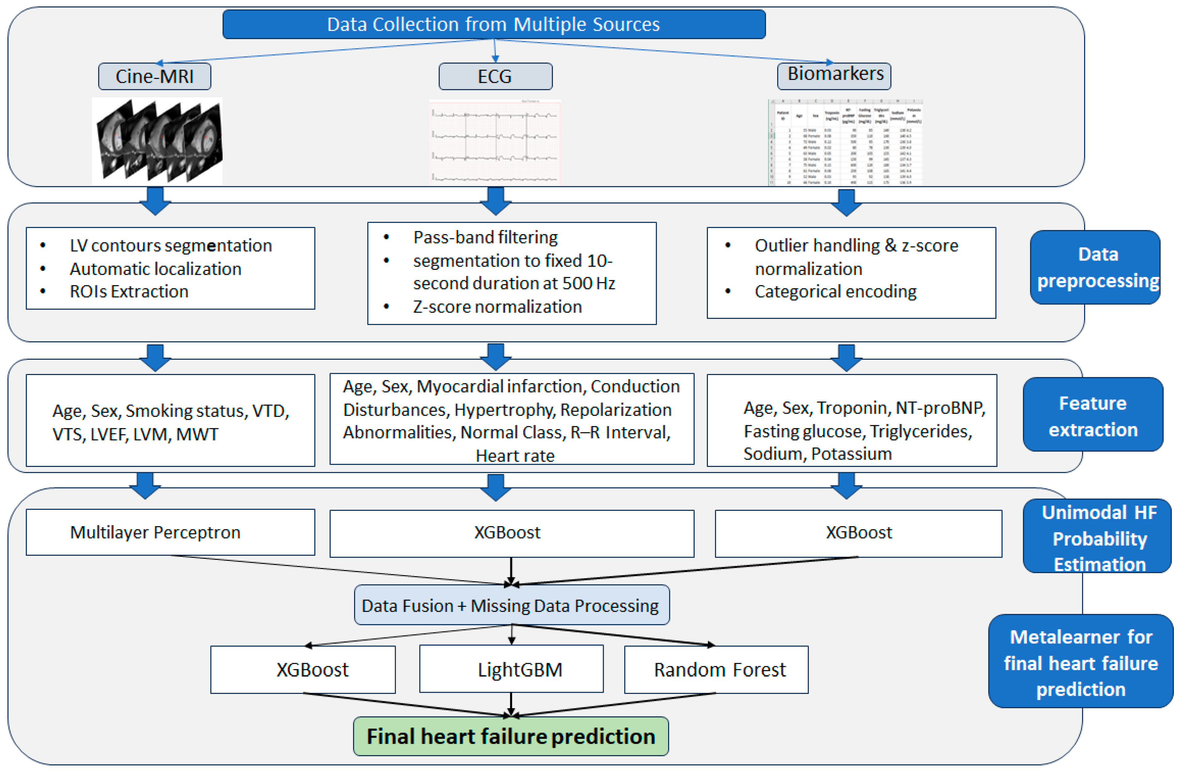
The present study aimed to develop and rigorously evaluate a hybrid meta-learning framework for HF diagnosis by combining predictions from independently trained cine-MRI, ECG, and biomarker models. The workflow comprises five sequential stages (Figure 1): (1) data collection, (2) preprocessing, (3) feature extraction, (4) unimodal probability estimation, and (5) final prediction through meta-learning fusion.
In this study, data were collected from three sources: cine-MRI sequences, 12-lead ECG recordings, and clinical biomarker profiles. During preprocessing, cine-MRI data were standardized to a fixed spatial resolution and temporal length. ECG signals were filtered using a pass-band filter (0.5–40 Hz), segmented into 10 s intervals at 500 Hz, and normalized using Z-score normalization. Biomarker data were processed by addressing missing values and outliers, normalizing continuous variables via Z-score, and converting categorical variables into numerical representations. Then, modality-specific features were derived from each data source to capture clinically relevant information.
In the unimodal probability estimation phase, independent predictive models generated probabilistic estimates of HF for each modality. These modality-specific probabilities were subsequently combined through a late-fusion meta-learning strategy, where the meta-learner integrated the available predictions into a Final Average HF Probability that served as the basis for the final diagnosis.
TRIPOD+AI Reporting: This study is reported in accordance with the TRIPOD+AI (Transparent Reporting of a Multivariable Prediction Model for Individual Prognosis or Diagnosis + Artificial Intelligence) statement. The completed TRIPOD+AI checklist is provided as Supplementary Material. All analyses and reporting follow the recommendations for AI-based clinical prediction models, ensuring transparency in model development, evaluation, and assessment of clinical utility.

3.2. Study Population and Eligibility Criteria

This study employs a late-fusion framework integrating three complementary diagnostic modalities: (1) cine-MRI, for high-resolution structural and functional assessment of the heart, (2) 12-lead ECG, for detailed electrophysiological characterization, and (3) biomarkers, for comprehensive molecular and metabolic profiling. This integrative framework addresses three core questions in cardiac assessment and heart failure prediction: Where?—through cine-MRI, enabling precise spatiotemporal mapping of cardiac structure and function; When?—through ECG recordings, providing accurate temporal characterization of electrical activation patterns; and Why?—through biomarker panels elucidating underlying molecular pathways and metabolic mechanisms.

3.2.1. Cine-MRI Imaging Cohort

Cine-MRI data were retrospectively collected from 281 patients (141 with heart failure and 140 healthy controls) at the Military Hospital of Tunis between 2021 and 2024. Each patient contributed 20–40 short-axis slices, yielding approximately 7000 anonymized images. Two groups were defined:
Healthy controls (target = 0) were rigorously screened to meet the following criteria: (1) left ventricular ejection fraction (LVEF) > 55% as measured by the Simpson’s biplane method; (2) no structural abnormalities on MRI; and (3) no clinical history of cardiovascular disease, hypertension, or diabetes. Normal sinus rhythm on resting ECG was confirmed when available.
Heart failure patients (target = 1) were defined by an LVEF below 50%, confirmed by MRI, and symptoms such as shortness of breath during exertion, fatigue, and reduced exercise capacity.
All HF diagnoses were clinically confirmed by an expert cardiologist. Cine-MRI parameters were independently verified by a blinded expert radiologist through manual tracing of left ventricular contours, serving as the reference standard. This dual-specialist validation ensured high diagnostic accuracy for both functional and structural assessments. Exclusion criteria included non-ischemic cardiomyopathies, severe valvular disease, congenital defects, or arrhythmia compromising image quality. Data handling adhered to the Declaration of Helsinki. All images were anonymized according to DICOM Supplement 142 with three adaptations: (1) the retention of patient age in metadata, (2) systematic shifting of birth dates to 1 January 1900, and (3) the removal of hospital identifiers while preserving scanner-specific technical tags.

3.2.2. Physionet ECG Database: Cohort Selection

ECG data were obtained from the publicly available PTB-XL dataset on PhysioNet, comprising 21,837 recordings from 18,885 patients collected at Charité University Hospital (Berlin, 1989–1996) [20]. Based on the diagnostic criteria described above, we identified 4378 patients with heart failure and 17,459 healthy controls. Each 12-lead ECG lasted 10 s, sampled at 500 Hz, and annotated with SCP-ECG and SNOMED-CT diagnostic codes. Two groups were extracted:
Healthy controls (target = 0) were defined by the absence of pathological ECG findings in all 12 leads, with physiological heart rate, PR/QRS/QT intervals, and QRS axis, and no conduction delays, repolarization abnormalities, or arrhythmias.
Heart failure group (target = 1) were identified by the presence of ECG abnormalities frequently associated with structural or functional cardiac dysfunction, prolonged QRS duration (>120 ms), left ventricular hypertrophy (LVH), atrial fibrillation and repolarization abnormalities such as ST changes. Patient age is provided as a continuous variable in years, while sex and other demographic information are encoded categorically. All recordings were anonymized prior to public release.
To prevent data leakage, all splits of the PTB-XL dataset were performed at the patient level, ensuring that recordings from the same patient were assigned exclusively to either the training or test set.

3.2.3. Biomarker Data Sources

The biomarker dataset was collected between 2024 and 2025 from the Biochemistry Laboratory of the Rabta University Hospital Center and comprises 157 patients including 94 patients with heart failure and 63 healthy controls. The cohort was stratified into two groups:
Healthy controls (target = 0): Individuals with no cardiovascular, metabolic, or renal disease and presenting biomarker values within normal physiological ranges. These subjects were further screened to exclude acute illness, pregnancy, or recent treatments known to significantly alter biomarker levels.
Heart failure patients (target = 1): A total of 94 patients with a confirmed diagnosis of heart failure, presenting abnormal values in key cardiac-specific markers such as NT-proBNP and troponin, as well as related metabolic markers including fasting glucose, triglycerides, sodium, and potassium, reflecting cardiac stress and systemic metabolic alterations. The dataset includes demographic information such as age and sex to enable stratification and subgroup analyses. All data were anonymized prior to analysis, and records with incomplete or implausible values were excluded.

3.3. Datasets Preprocessing

3.3.1. Cine-MRI

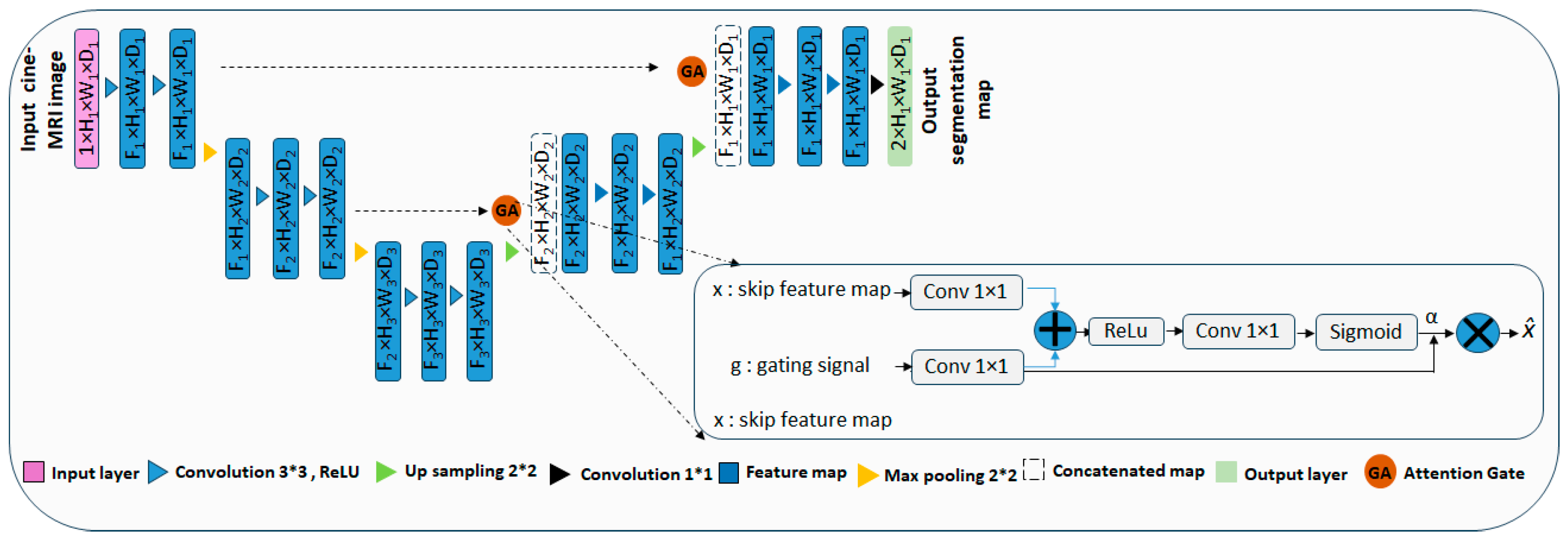
Although reference contours were available, relying on them would limit generalizability to unannotated datasets. Automatic segmentation is therefore essential to ensure robustness and reproducibility. To address this limitation, we propose a lightweight Attention U-Net which follows the typical encoder–decoder structure of the original U-Net [21], while integrating attention gates at the skip connections. The model comprises three down sampling and three up sampling stages. Each encoder stage includes two convolutional blocks, each followed by a ReLU activation and a max-pooling operation. The decoder mirrors this configuration, employing transposed convolutions for up sampling and additional convolutional layers for feature refinement. Skip connections transfer spatial information between the encoder and decoder, while the attention mechanism selectively enhances relevant features before fusion. The overall architecture of the proposed Attention U-Net is depicted in Figure 2. The lightweight Attention U-Net was trained in a supervised manner using reference contours, with a composite loss function combining cross-entropy and Dice losses. The dataset was divided into 80% for training, 10% for validation, and 10% for testing. To eliminate manual intervention during post-processing, left ventricle (LV) localization was automated based on the contours generated by Attention U-Net. For each slice, the geometric center of the epicardial contour was calculated to define the ROI. This centroid-based approach ensures consistent ROI positioning within the ventricular region, regardless of inter-patient or inter-slice variations in shape and orientation.
Mathematically, the epicardial contour is represented as a set of points (xi,yi); the centroid (xc,yc) is defined as follows:
x c = 1 N i = 1 N x i ,       y c = 1 N i = 1 N y i
where N represents the total number of contour points. Using the computed centroid as the center, a square ROI was defined to consistently capture the myocardial region. Each ROI was then resized to 128 × 128 pixels to ensure e spatial normalization and reproducibility across all patients and slices.

3.3.2. ECG Dataset

The ECG signals from the PTB-XL dataset were preprocessed to ensure consistency and high signal quality prior to model integration. All recordings were standardized to a duration of 10 s with a sampling frequency of 500 Hz. When necessary, signals were truncated or zero-padded to meet this specification. To reduce baseline wander and high-frequency noise, a band-pass filter with cut-off frequencies of 0.5–40 Hz was applied. The filter response in the frequency domain is defined as follows:
H f = 1     if   0.5   f 40 0     otherwise .
After filtering, each ECG recording was normalized using Z-score normalization to minimize inter-subject variability and ensure consistency across the dataset. For a given ECG signal x = [x1, x2, …, xN], the normalized signal xi′ is computed as follows:
x i = x i μ σ ,   i = 1 , 2 , , N
where μ and σ denote the signal’s mean and standard deviation, defined, respectively, as follows:
μ = 1 N i = 1 N x i ,   σ = 1 N i = 1 N ( x i μ ) 2 .
This normalization centers each ECG recording around zero and scales it to unit variance, thereby mitigating amplitude differences while preserving the morphological characteristics of the waveform. Such preprocessing ensures signal comparability across patients and facilitates robust neural network training. Furthermore, the PTB-XL database provides manually reviewed R-peak annotations. Only normal-to-normal (NN) intervals were retained to ensure high-quality signals for subsequent feature extraction.

3.3.3. Biomarker Data Sources

The biomarker dataset was preprocessed to ensure consistency and suitability for model training. Outliers were addressed through truncation or median imputation to reduce their impact on subsequent analyses. Continuous biomarkers, including troponin and NT-proBNP, were standardized using Z-score normalization to facilitate robust neural network training while preserving diagnostically relevant variations. Categorical variables, such as sex, were encoded numerically (e.g., Male = 0, Female = 1) to ensure uniform representation. These preprocessing steps standardize the biomarker data and enhance comparability across patients, thereby enabling their effective integration into the predictive framework.

3.4. Feature Extraction

3.4.1. Cine MRI Dataset

From cine-MRI, five cardiac-specific metrics were extracted: end-diastolic volume (EDV), end-systolic volume (ESV), left ventricular ejection fraction (LVEF), myocardial wall thickness (MWT), and myocardial mass. In addition to these MRI-derived features, three demographic variables (age, sex, and smoking status) were also included as predictive features in the model. Table 2 provides a detailed summary of the extracted features, including their definitions, typical values, and clinical relevance for predicting HF.
All cardiac parameters listed in Table 2 were automatically computed from short-axis cine-MRI sequences using a dedicated processing pipeline. MWT was calculated from left ventricular contours extracted using a lightweight Attention U-Net. It is defined as the distance between endocardial and epicardial boundaries across all cardiac phases, thereby capturing subtle structural variations. Left ventricular volumes were estimated by integrating both spatial and temporal information from cine-MRI sequences. Rather than relying solely on static slice thickness, this method utilized pixel displacement across successive cardiac phases, enabling the estimation of instantaneous ventricular volumes by multiplying the endocardial surface area by the corresponding spatial distance. EDV and ESV were then obtained as the maximum and minimum volumes across the cardiac cycle, respectively. The LVEF was calculated as follows [22]:
L V E F = E D V E S V E D V × 100
Myocardial mass was determined from the difference between epicardial and endocardial volumes, scaled by the specific density of myocardial tissue (1.05 g/mL).

3.4.2. ECG Dataset

Most ECG features used in this study were provided by the PTB-XL dataset. These include diagnostic categories such as myocardial infarction, conduction disturbances, hypertrophy, repolarization abnormalities, and normal rhythm classification (Table 3). Demographic variables (age and sex) were also included as predictive features.
To enhance these attributes, the R–R interval was automatically extracted from all recordings to capture rhythm-related characteristics relevant to heart failure prediction. Heart rate was subsequently derived from these intervals. Both features were computed using the Pan–Tompkins QRS detection algorithm, resulting in a total of 9 ECG features for analysis. This approach integrates morphological, temporal, and diagnostic information, providing a comprehensive electrophysiological profile for the predictive model.

3.4.3. Biomarker Data Sources

Table 4 provides a detailed description of the biomarker features, including their typical reference ranges and clinical relevance. In addition to these biochemical markers, demographic variables (age and sex) were also included as predictive features in the model. Given the limited number of clinically meaningful features, their inclusion does not substantially increase model complexity or introduce redundancy. Retaining all variables ensures an unbiased and comprehensive representation of the patient’s physiological and metabolic profile. This approach is particularly relevant as each modality is processed and trained independently prior to multimodal integration, thereby maximizing the contribution of each feature set to the overall predictive performance.

3.5. Proposed Multimodal Late-Fusion Framework for Heart Failure Prediction

The proposed multimodal framework integrates complementary information from three independent modality-specific data sources to produce a single, clinically interpretable prediction of HF. Rather than processing raw data directly, each modality branch receives pre-extracted, modality-specific features as described in Section 3.4. Each branch transforms its input features into probabilistic outputs using a modality specific model: a multilayer perceptron (MLP) for cine-MRI features, and XGBoost classifiers for ECG and biomarker features. These unimodal predictions are then combined through a late fusion meta-learner. Among several tested fusion strategies, the final HF probability was obtained by averaging the calibrated outputs of the individual models, ensuring a robust and balanced prediction across modalities.

3.5.1. MRI-Based Branch

a.
Feature preparation
Demographic variables (age, sex, smoking status) and MRI-derived cardiac parameters (myocardial wall thickness, ventricular volumes, myocardial mass) were organized into a structured table with patients as rows and features as columns. To prevent biases arising from differences in units and ranges, continuous features were normalized across patients using Min-Max scaling, transforming values to the [0, 1] range while preserving relative differences defined as follows [23]:
X N o r m a l i z e d = X X m i n X m a x X m i n
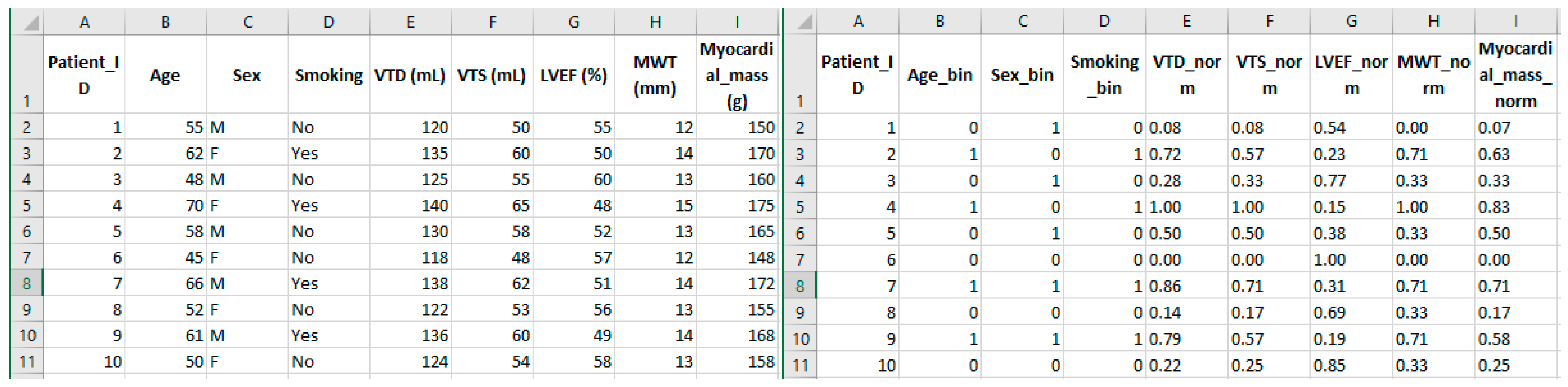
where X denotes the original feature value, and Xmin and Xmax are the cohort-wide minima and maxima, respectively. Categorical variables, including sex and smoking status, were encoded as binary features (0/1). Age was dichotomized into two categories, 18–59 years (0, lower risk) and ≥60 years (1, higher risk), to incorporate demographic risk factors consistently within the neural network framework. Figure 3 illustrates the effects of Min-Max scaling on feature distributions for a subset of patients, highlighting transformation into dimensionless, comparable inputs.
Following normalization and encoding, patient-specific feature vectors were concatenated into fixed-order, one-dimensional arrays. Stacking these vectors across all patients yielded a standardized two-dimensional input matrix (npatients,nfeatures) for the perceptron-based model.
b.
MLP-Based Prediction Framework
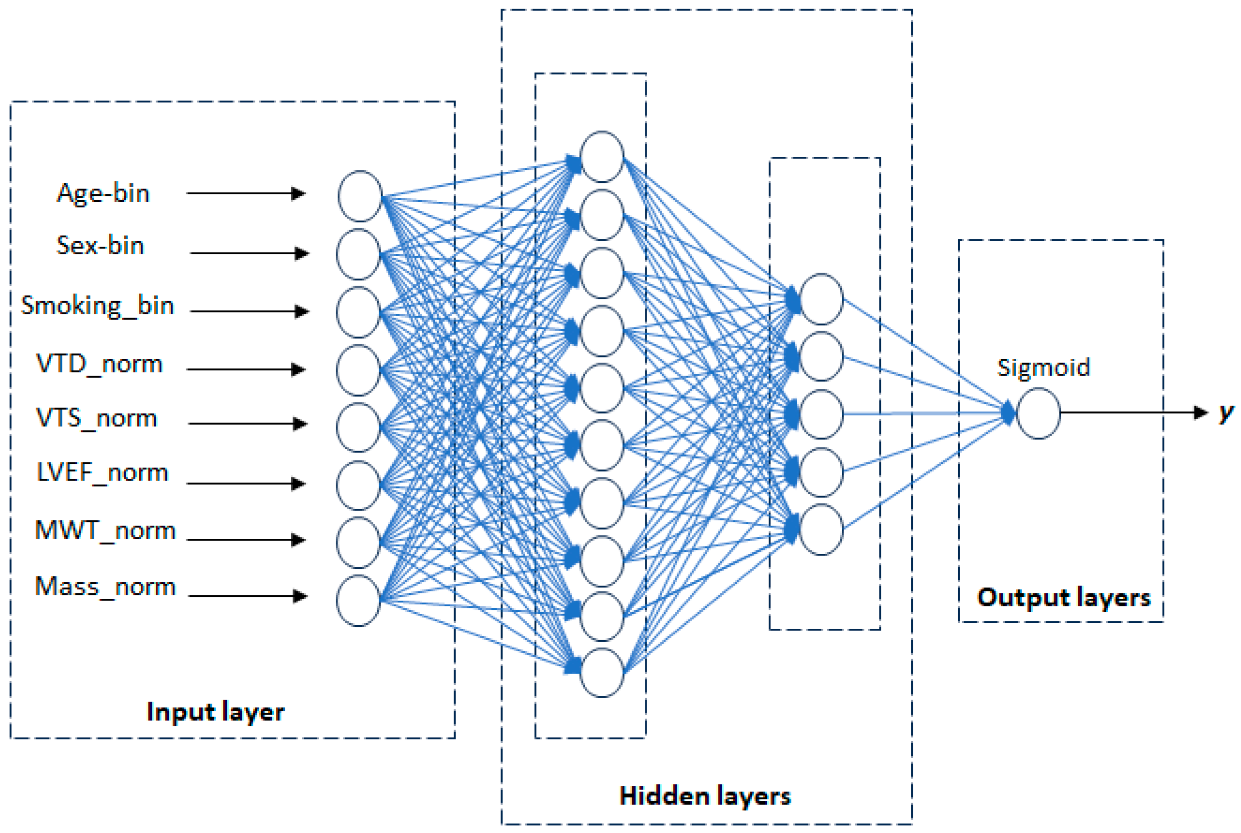
The MRI branch employs a multilayer perceptron (MLP) to process 8 normalized features derived from cine-MRI and demographic data. The MLP architecture (Figure 4) comprises an input layer with eight neurons and two hidden layers containing 10 and 5 neurons, both using Rectified Linear Unit (ReLU) activations and a single sigmoid output neuron producing the HF probability y [24]:
y = σ z = 1 1 + e z
The model was trained using 80% of the dataset with internal validation, and the remaining 20% was reserved for independent testing. Optimization strategies (Adam and Adamax) and mini-batch sizes (8 and 16) were compared to identify the optimal training configuration. Training performance was evaluated via mean squared error (MSE) [23]:
M S E = 1 N i = 1 N ( y i t i ) 2
where yi denotes predicted probabilities and ti the corresponding target values. During testing, the network weights were fixed, and the trained MLP was applied to the test features to generate probability estimates of HF for unseen samples. After training and validation, the model’s sigmoid outputs (y) were calibrated using Platt scaling to improve the alignment between predicted and observed probabilities. This approach applies a logistic regression model to the raw MLP outputs, generating calibrated probabilities y′ that more accurately represent the true likelihood of HF and provide reliable inputs for the subsequent meta-learner, calculated as follows:
y = 1 1 + e ( a y + b )
where a and b are parameters learned on the validation set. For cine-MRI-derived features, an MLP was chosen for its ability to model a small, dense set of continuous tabular features and capture complex non-linear and hierarchical relationships among clinically relevant measurements (e.g., volumes, ejection fraction, mass). Its probabilistic outputs provide well-calibrated estimates of heart failure risk, enabling seamless integration into the multimodal meta-learning framework. Compact architecture ensures computational efficiency, reduces overfitting, and preserves interpretability, allowing for meaningful clinical insights from the learned feature representations.

3.5.2. ECG-Based Branch

a.
Feature preparation
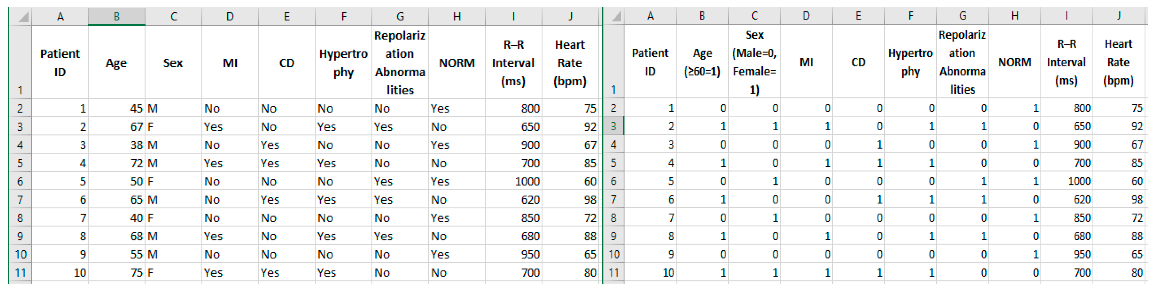
ECG-derived features were prepared for predictive modeling by encoding age into two categories (<60 years = 0, ≥60 years = 1) to reflect increased HF risk with age, and encoding sex as a binary variable (male = 0, female = 1). Clinical features were encoded as binary indicators (1 = presence, 0 = absence). Continuous electrophysiological features, including the R–R interval (600–1200 ms) and Heart Rate (50–100 bpm), were retained as numerical values. For this study, an XGBoost classifier was employed for prediction. As a tree-based model relying on threshold-based splits rather than distance or gradient magnitude, XGBoost does not require normalization of continuous variables. All features were organized into a structured dataset, with rows representing patients and columns representing features to ensure consistent input for prediction (Figure 5).
b.
XGBoost-Based Prediction Framework for ECG Features
For the ECG branch, we employed the Extreme Gradient Boosting (XGBoost) algorithm, an ensemble of shallow decision trees (depth 3–5) trained sequentially to correct predecessor errors. This approach captures complex interactions among the nine ECG features while ensuring robust probabilistic outputs. Hyperparameter optimization was conducted using a simple grid search over three representative values for each key parameter, including n_estimators, max_depth, learning_rate, subsample, colsample_bytree, reg_alpha, reg_lambda, min_child_weight, gamma and scale_pos_weight. Five-fold cross-validation was performed within the training set to ensure robust and efficient evaluation of each parameter configuration. For a given a dataset D = ( x i , y i ) ( D = n , x i ϵ R 9 , y i ϵ 0 , 1 ) , where xi represents the 9 ECG features and yi the binary label (1 for heart failure, 0 otherwise), the model generates a continuous output score for each patient, which is transformed into a probability estimate for heart failure using the logistic function [25]:
P ( y i = 1 | x i ) = 1 1 + e ( x i )
where x i = k = 1 K f k x i , with f k ϵ F representing the ensemble of decision trees.
The objective function optimizes the binary logistic loss with regularization [26]:
L = i l y h a t i , y i + k Ω ( f k )
with Ω f = γ T + 1 2 λ ω 2 , where T is the number of leaves in the tree and ω is the vector of leaf scores.
The dataset was split into training (80%) and testing (20%) sets, ensuring a balanced representation of patients with and without HF. The model was trained on the training set using the optimized hyperparameters, and performance was evaluated on the held-out test set, providing probabilistic predictions for each patient. The model, trained using optimized hyperparameters, was then evaluated on the test set to generate probabilistic predictions for each patient. Unlike individual decision trees, XGBoost constructs an ensemble of weak learners sequentially, each focusing on correcting the errors of its predecessors. This iterative refinement improves predictive accuracy and generalization. Feature splitting prioritizes partitions that maximize discrimination between HF and non-HF cases, while regularization terms control model complexity and prevent overfitting. For ECG features, XGBoost was selected for its ability to handle heterogeneous data types and clinically meaningful thresholds. The algorithm natively accommodates missing values without requiring feature scaling, making it well suited for the heterogeneous and partially incomplete nature of the ECG dataset. Its regularization mechanisms further enhance robustness and reduce the risk of overfitting in a moderate-sized cohort.
Once preprocessing was complete, the features were directly input into the trained XGBoost model to generate probabilistic predictions quantifying each patient’s likelihood of HF [27].

3.5.3. Biomarker-Based Branch

a.
Feature preparation
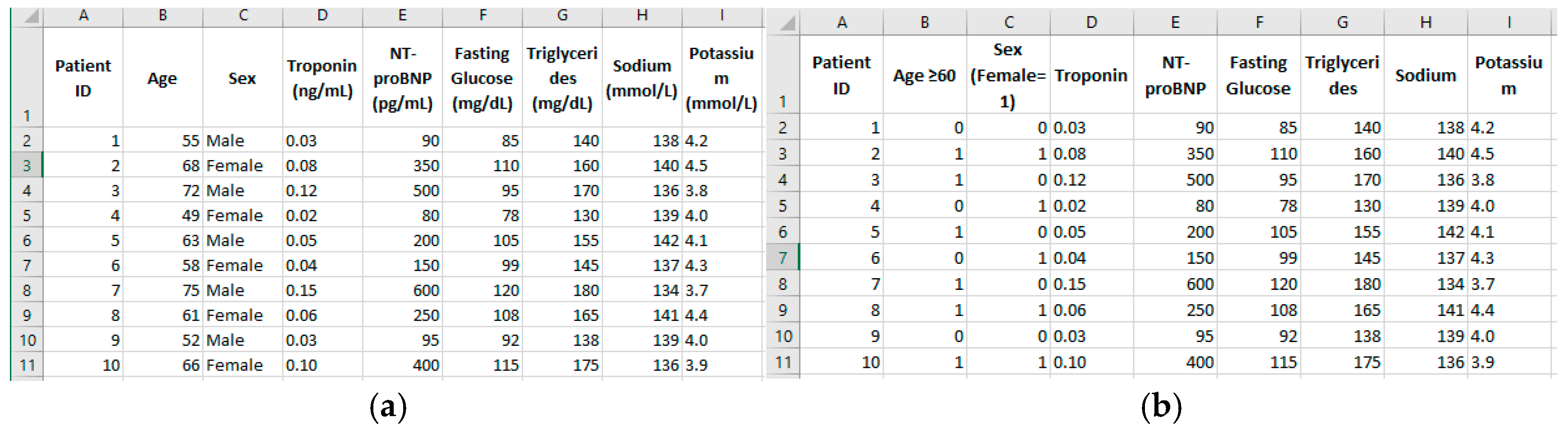
To ensure consistency across datasets, sex was encoded as a binary variable (male = 0, female = 1) and age was binarized at 60 years (<60 = 0, ≥60 = 1). The remaining six biochemical features including troponin, NT-proBNP, fasting glucose, triglycerides, sodium and potassium were retained in their original units to preserve their clinical meaning and ensure compatibility with the XGBoost algorithm, which does not require feature scaling. Figure 6 illustrates the feature values for ten patients before and after preprocessing, demonstrating demographic encoding and preservation of continuous biochemical markers.
Theorem-type environments (including propositions, lemmas, corollaries, etc.) can be formatted as follows:
b.
XGBoost-Based Prediction Framework for Biomarker Features
The biomarker branch employed the XGBoost algorithm to predict heart failure using 8 tabular features, including binarized age, encoded sex, and six continuous biochemical markers. XGBoost was chosen for its strong suitability for heterogeneous clinical tabular data, which often include mixed feature types, varying value scales, and clinically meaningful threshold. Tree-based boosting models naturally capture non-linear interactions and decision boundaries driven by biochemical cut-offs (e.g., elevated NT-proBNP levels), closely aligning with clinical reasoning. The model architecture was initialized with 300 boosting rounds, a maximum tree depth of 4, a learning rate of 0.01, subsample and colsample_bytree ratios of 0.6, and moderate L1/L2 regularization to control model complexity. A simplified grid search evaluated two additional values per hyperparameter to optimize performance while mitigating overfitting. A binary logistic objective was used to directly generate continuous probability scores, without requiring additional calibration.
The dataset was split into 80% training data (125 patients), which included internal validation during hyperparameter tuning, and 20% independent testing data (32 patients), maintaining balanced representation between heart failure patients and controls.

3.5.4. Multimodal Late Fusion and Meta-Learning Strategy

a.
Preparation of Multimodal Features for Meta-learner
The core idea behind the meta-learning strategy is to combine the probability estimates generated by multiple modality-specific models into a unified decision framework for HF prediction. By integrating complementary predictions, the meta-learner exploits the complementary diagnostic information provided by each modality, thereby enhancing robustness and the clinical relevance of the final prediction. A key challenge in this framework is that the cine-MRI, ECG, and biomarker models were trained on distinct patient cohorts, which prevents direct patient-level fusion of their predictions and necessitates a dedicated meta-learning strategy. In routine clinical practice, patients do not systematically undergo cine-MRI, ECG, and biomarker profiling within a single episode of care. These examinations are typically performed across distinct hospital services including radiology, cardiology and biochemistry—each with its own scheduling constraints, equipment availability, and clinical indications. Consequently, aligning patient-level data retrospectively would have required a coordinated prospective protocol, which was beyond the scope of this study. This practical limitation is, in fact, a common challenge in real-world clinical data integration and strongly motivated our choice of a late-fusion strategy. Thus, the proposed framework is presented as a cohort-pooling feasibility analysis, integrating cohort-specific predictions at the decision level. To address this issue, the meta-learner was designed to mimic clinical practice by integrating available probabilistic outputs from cine-MRI, ECG, or biomarkers. This design enables flexible and clinically realistic decision-making even when some modalities are unavailable.
Rather than inputting missing values, we adopted a strategy that enables the meta-learner to handle missing information directly. It uses modality-specific availability indicators (has_IRM, has_ECG, has_Bio) together with the corresponding predicted probabilities. For unavailable modalities, probabilities are assigned a neutral placeholder value (p = 0.5), while the indicator ensures that these values are effectively disregarded by the model. In this way, the meta-learner is trained to rely on the predictive contribution of a modality only when its indicator equals 1 and to ignore it otherwise. This mechanism allows the model to adaptively rely on available modalities, ensuring flexibility and robustness despite missing data. The resulting dataset combines each patient’s available modality probabilities with their corresponding presence indicators forming the input for the meta-learner.
The modality-specific models generate probability estimates in the [0, 1] range, which are inherently normalized and comparable across modalities, regardless of the heterogeneity of the original data sources. This property ensures that the meta-learner receives inputs that are consistent and suitable for integration, even when the underlying data originate from different institutions, populations, or acquisition protocols.
b.
Meta-learner selection
For the final HF prediction, we considered several established machine learning algorithms that meet two key methodological requirements in a multimodal clinical context: robustness to heterogeneous and partially missing data, and the ability to automatically weight features according to their predictive relevance. Accordingly, we focused on tree-based ensemble learners, which are well suited to the practical constraints of real-world multimodal data and the need for stable probability estimation. Based on both state-of-the-art review and empirical suitability for tabular multimodal fusion, three complementary models were selected as meta-learners: XGBoost, LightGBM, and Random Forest. These algorithms natively handle heterogeneous clinical inputs, accommodate mixed data types without feature scaling, and incorporate intrinsic mechanisms for feature importance estimation and regularization, reducing the risk of overfitting. Their tree-based structure also enables threshold-based decision modeling that aligns with clinical reasoning. In contrast, alternative approaches such as support vector machines or neural network-based meta-models were not retained, as they generally require extensive preprocessing to handle missing values and lack intrinsic, adaptive feature importance, which is critical for stable fusion of multimodal probability outputs.
  • XGBoost:
The XGBoost algorithm follows the ensemble of decision trees principle described in Section 3.5.2, where each tree incrementally corrects errors from prior iterations to optimize the binary logistic objective. In this study, it was chosen for its efficiency, scalability, and robust regularization strategies, which help prevent overfitting while maintaining high predictive accuracy in heterogeneous datasets. For features with missing entries, XGBoost learns a default split direction during training rather than requiring imputation. Let a candidate split on feature j have threshold τ, and let Gain(dir) denote the split gain if missing values are assigned to a branch (dir), where L and R indicate left and right branches, respectively. The optimal direction is as folows:
d i r * = arg   max   G a i n ( d i r )
This enables effective handling of missing modality information during tree construction, with each leaf’s predicted score computed from the gradients (G) and Hessians (H) of its observations as follows:
w * = G H + λ
where G = i g i and H = i h i over the leaf samples. This formula shows how XGBoost automatically assigns more weight to observations that are more informative, allowing the model to adaptively focus on critical inputs.
  • LightGBM:
LightGBM shares the same objective function as XGBoost, optimizing the binary logistic loss with regularization on leaf scores to produce probabilistic outputs for HF prediction. A key distinction lies in its leaf-wise tree growth strategy, which selects splits to maximize gain, allowing for deeper leaves where data variance is higher. LightGBM selects the best split point s* by minimizing the following [28]:
S * = arg   min [ G l e f t 2 H l e f t + λ + G r i g h t 2 H r i g h t + λ G t o t a l 2 H t o t a l + λ ]
where Gleft, Gright are gradient sums for left and right child nodes. Hleft, Hright are Hessian sums. λ is a regularization parameter. This leaf-wise strategy efficiently handles heterogeneous features and missing values by optimizing splits on observed data, making LightGBM well suited for our multimodal dataset.
  • Random Forest:
Random Forest (RF) is tree-based approach that aggregates multiple decision trees, each trained on a bootstrap sample and using a random subset of features to determine splits, thereby enhancing robustness and reducing overfitting. This ensemble method naturally handles missing values by employing surrogate splits or directing observations with missing features to the most appropriate branch, enabling reliable predictions even when some modality probabilities are unavailable. The final output is obtained by averaging the predicted probabilities from all trees:
P y i = 1 x i = 1 T t = 1 T f t ( x i )
where ft(xi) represents the probability predicted by the tth tree and T is the total number of trees in the ensemble.
c.
Meta-Learner Training and Final Prediction
For meta-learner training, we applied a sample weighting strategy to address imbalance in modality representation. Each patient was assigned a weight inversely proportional to the size of their available modality. This ensured that no single modality dominated the loss function during training. The meta-dataset was randomly split into 80% for training (with internal validation) and 20% for testing. This split preserved evaluation integrity and allowed the model to learn effectively from incomplete multimodal data.
To prevent data leakage, all probability estimates used for meta-learner training were generated exclusively from the training splits of each modality-specific model. The meta-learner was then evaluated on the held-out test set, ensuring that no information from the test data was used during training or validation. This strict separation is also illustrated in Algorithm 1, which provides a step-by-step overview of the entire pipeline.
Following the training of the three meta-learners (XGBoost, LightGBM, and Random Forest), we combined their outputs using ensemble averaging. For each patient, the final HF probability was computed by averaging the three predicted probabilities, enhancing robustness and leveraging each algorithm’s strengths, as shown in the following equation:
P f i n a l i = P X G B o s s t i + P L i g h t G B M i + P R a n d o m   F o r e s t ( i ) 3
where pfinal(i) represents the consolidated risk estimate for patient i. All experiments were performed on a system equipped with an Intel Core i7 CPU and 64 GB of RAM, providing sufficient computational resources for model training and evaluation. Algorithm 1 summarizes the complete multimodal prediction pipeline integrating cine-MRI segmentation, ECG and biomarker analysis and meta-learner fusion to generate final HF risk probabilities.
Algorithm 1 Heart Failure Prediction Using Multimodal Data and Meta-learner
#Inputs:
  • Cine-MRI images for a set of patients PMRI
  • ECG data for a set of patients PECG
  • Biomarkers data for a set of patients PBio
  • Patient labels y ∈ {0,1} for heart failure
#Output: Final prediction probability for heart failure for each patient

Step 1: Train individual modality models
for each modality m ∈ {Cine-MRI, ECG, Biomarkers} do

    if m == Cine-MRI then
          Perform segmentation using U-Net
              Calculate D S C = 2 T P 2 T P + F P + F N × 100
           Calculate   H D = m a x ( max p C A   d p , C B , max q C B d q , C A
          Extract features and train MLP classifier
          output probability p-MRI
    else If m == ECG then
          Extract temporal and frequency features
          Train XGBoost with objective function: L = Σ y log p + 1 y log 1 p + Ω f
           where   Ω f = γ T + ½ λ w 2
          output probability p_ECG
    else if m == Biomarkers then
          Train XGBoost similarly
          output probability p_Bio
    end if

end for

Step 2: Dataset preparation and splitting for meta-learner

#Input: All patients P=PMRI ∪ PECG ∪ PBio

for each patient i in P do
Initialize   feature   vector   v e c t o r i m e t a = [ N a N , N a N , N a N ] ,
      if i ∈ PMRI then
             v e c t o r i m e t a = [ 0 ] ← pMRI (i)
      end if
      if i ∈ PECG then
             v e c t o r i m e t a = [ 1 ] ← pECG (i)
      end if
      if i ∈ PBio then
             v e c t o r i m e t a = [ 2 ] ← pBio (i)
      end if
Store target yi ← heart failure label of patient i
end for

# Shuffle P randomly
      Ptrain = first 80% of P
      Ptest = remaining 20% of P

# Calculate training weights:
      NMRI = count of MRI patients in Ptrain
      NECG = count of ECG patients in Ptrain
      NBio = count of Bio patients in Ptrain
      Ntotal = ∣Ptrain
# Normalize weights so that the sum of weights for each modality is that the total sum of weights is the number of patients

for each patient i ∈ Ptrain do
  wi = 0
    if has MRI then
          wi + = Ntotal/(3×NMRI)
    end if
    if has ECG then
          wi+ = Ntotal/(3×NECG)
    end if
    if has Bio then
          wi + = Ntotal/(3×NBio)
    end if

end for

#Output

(Xtrain,ytrain,wtrain) for Ptrain
(Xtest,ytest) for Ptest

Step 3: Meta-learner Training

#Input: (Xtrain, ytrain, wtrain)

# Initialize three metalearners:
      ML1 ← XGBoost
      ML2 ← LightGBM
      ML3 ← Random Forest
for each meta-learner ML ∈ [ML1, ML2, ML3] do

      Train ML on (Xtrain, ytrain) (Xtrain, ytrain) with sample weights wptrain
end for

#Output: Three trained meta-learner models
Step 4: Final Prediction Generation

Inputs:
  Trained meta-learners:
      ML_XGBoost
      ML_LightGBM
      ML_RandomForest
  Test set:
      P_test with feature vectors X_test

for each patient i ∈ P_test do

    Get prediction from XGBoost:
    p_xgb = ML_XGBoost.predict_proba(x_i)

  Get predictions from LightGBM:
  p_lgb = ML_LightGBM.predict_proba(x_i)
  Get predictions from Random Forest:
  p_rf = ML_RandomForest.predict_proba(x_i)

  Compute final ensemble prediction:
  p_final(i) = (p_xgb + p_lgb + p_rf)/3
end for
#output
Final ensemble prediction probabilities p_final

Step 5: Performance evaluation
Inputs
       True labels y_test for P_test
       Final predictions p_final for P_test
       Calculate AUC-ROC
       AUC = roc_auc_score(y_test, p_final)
       Calculate key metrics for comparison with state-of-the-art methods
       Accuracy = (TP + TN)/(TP + TN + FP + FN)
       Sensitivity =TP/(TP+FN)
       Precision = TP/(TP + FP)
       Recall = TP/(TP + FN)
       F1 = 2 × (Precision × Recall)/(Precision + Recall)
outputs
       Primary metrics for state-of-the-art comparison: AUC, F1-score, Accuracy
       Clinical performance metrics: Precision, Recall, Specificity

3.6. Performance Evaluation

The performance of the proposed multimodal framework was evaluated at multiple stages to ensure the robustness and interpretability of each component.
The segmentation performance of cine-MRI images was first assessed using the Dice Similarity Coefficient (DSC) and the Hausdorff Distance (HD), two widely adopted metrics in medical image analysis. The DSC quantifies the spatial overlap between the predicted (CA) and ground-truth (CB) contours, while the HD measures boundary agreement by computing the maximum surface deviation between the two sets. They are defined as follows [29]:
D S C ( % ) = 2 T P 2 T P + F P + F N × 100
HD = max (max p ⸦ CA d (p, CB), max q ⸦ CB d(q, CA))
where TP, FP, and FN denote the true positive, false positive, and false negative pixels, respectively.
For the evaluation of individual modality predictions, the MLP (cine-MRI), XGBoost (ECG), and XGBoost (biomarkers) models were assessed using several complementary metrics. These included the Area Under the Receiver Operating Characteristic Curve (AUC–ROC), Mean Squared Error (MSE), and Brier Score, which jointly measure discrimination and calibration performance. To facilitate comparison with state-of-the-art approaches, binary classification between HF and non-HF groups was performed across varying decision thresholds. Classical classification measures, including Accuracy, Precision, Recall, F1-score, Specificity, Positive Predictive Value (PPV), and Negative Predictive Value (NPV) were calculated according to the following equations [29]:
A c c u r a c y % = T P + T N ( T P + T N + F P + F N ) × 100
S e n s i t i v i t y = T P ( T P + F N )
R e c a l l = T P ( T P + F N )
F 1 -score = 2 × P r e c i s i o n × R e c a l l P r e c i s i o n + R e c a l l  
S p e c i f i c i t y = T N T N + F P
P P V = T P T P + F P
N P V = T N T N + F N
where TP (True Positive) represents patients correctly predicted as having HF, TN (True Negative) represents patients correctly predicted as not having HF, FP (False Positives) represent patients incorrectly predicted as having HF, and FN (False Negative) represents patients incorrectly predicted as not having HF.
In our study, the sample size was determined based on data availability. Following the ‘10 events per predictor variable’ (EPV) rule, the number of HF events in each cohort exceeds the minimum required for reliable model development: MRI: ≈17.6 EPV; ECG: ≈486 EPV; biomarkers: ≈11.75 EPV.
Since the computation of these metrics requires a decision threshold, an optimal value was determined using Youden’s index (J) on the validation set. This criterion balances sensitivity and specificity in a single score, ensuring that HF patients are correctly identified (high sensitivity) while reducing FP among healthy individuals (high specificity). The resulting threshold was then fixed and applied to the independent test set to obtain the final performance metrics. The index is expressed as follows:
J = S e n s i t i v i t y + S p e c i f i c i t y 1
In accordance with the TRIPOD+AI recommendations, all primary diagnostic performance metrics, including the AUC, accuracy, sensitivity, specificity, positive predictive value (PPV), negative predictive value (NPV), and F1-score, are reported together with their corresponding 95% confidence intervals (95% CIs), estimated from the independent test set. Confidence intervals were computed using DeLong’s method for AUC, Clopper-Pearson intervals for proportions, and patient-level bootstrap resampling for continuous metrics.
Additionally, a confusion matrix is provided at the optimal threshold to present the model’s performance transparently. The calibration of the probabilistic outputs is assessed visually using a calibration plot and quantitatively by reporting the calibration intercept and slope.

4. Experimental Results

4.1. Left Ventricle Segmentation

Hyperparameter tuning was performed to optimize the performance of the proposed Attention U-Net. The model was trained using Adam and Adamax optimizers with mini-batch sizes of 8 and 16, and learning rates of 10−2, 10−3, and 10−4. Training accuracy and validation loss were continuously monitored, and convergence was defined by plateauing accuracy and stable validation loss. The optimal configuration was selected based on validation set performance, and final metrics were evaluated on the independent test set (Table 5).
Across all configurations, Adamax consistently outperformed Adam, while a learning rate of 10−3 with a batch size of 8 achieved the highest segmentation accuracy. Under this configuration, performance improved steadily with the number of epochs, reaching a peak accuracy of 97.25% at 80 epochs. These results confirmed the effectiveness of the selected hyperparameters for the final U-Net architecture. Table 6 presents representative endocardial and epicardial segmentation results for a healthy subject and an HF patient.
The proposed model achieved consistently high accuracy across ventricular regions, with slightly higher DSC and lower HD values observed in mid-ventricular slices. Comparable results between healthy and HF cases further demonstrate the robustness and generalization of the proposed segmentation pipeline.

4.2. Heart Failure Prediction from Cine-MRI Features

This section reports the optimization and performance of the MLP-based framework for predicting HF probabilities from MRI-derived features. Table 7 summarizes the MSE values across combinations of learning rates, optimizers, network depths, epochs, and batch sizes.
Analysis of Table 7 shows that the MLP achieved its lowest MSE using two hidden layers, a learning rate of 10−2, and the Adamax optimizer. A batch size of 8 provided more stable convergence and lower errors compared to 16, while extending training beyond 100 epochs yielded no further improvement and occasionally increased MSE, suggesting overfitting.
The final optimized configuration, combining these parameters, achieved the best overall performance with minimal error. Table 8 presents representative predicted HF probabilities before and after Platt calibration, demonstrating the improved reliability and interpretability of the probabilistic outputs. The calibrated results reduced over- and under-estimations, ensuring well-calibrated and robust probability estimates.

4.3. Heart Failure Prediction from ECG Features

In this section, we present the predicted HF probabilities derived from ECG features using the proposed XGBoost model, focusing on the reliability of its probabilistic outputs. A grid search with five-fold cross-validation was performed over key hyperparameters to determine the optimal configuration, with performance assessed using the average MSE and log-loss across the validation folds. Table 9 presents the tested hyperparameter values and the corresponding optimal configuration.
The optimized configuration achieved a balanced trade-off between model complexity and generalization with a maximum depth of 4, 100 estimators, and a learning rate of 0.1. Regularization parameters (reg_α = 0.1, reg_λ = 1.5) and subsampling ratios (0.8 for rows and columns) enhanced robustness and prevented overfitting. The resulting model achieved strong and consistent predictive performance across the five validation folds with an average MSE of 0.042 ± 0.005 and log-loss of 0.15 ± 0.02, confirming its reliability in estimating HF probabilities from ECG features.

4.4. Heart Failure Prediction from Biomarkers Features

The biomarker-based XGBoost model was evaluated through a similar grid-search optimization using five-fold cross-validation. Table 10 presents the tested hyperparameters and highlights the configuration yielding the lowest error. The optimized XGBoost model achieved robust predictive performance for HF probability estimation from biomarker features, with an MSE of 0.038 and a log-loss of 0.172, reflecting accurate and well-calibrated outputs. The final configuration with 80 estimators, a depth of 3, a learning rate of 0.05, and regularization (L1 = 0.1, L2 = 2) balanced model complexity and generalization.

4.5. Final Meta-Learner-Based Heart Failure Prediction

This section evaluates three meta-learner architectures that integrate modality-specific probability estimates from the cine-MRI, ECG, and biomarker branches through a late-fusion strategy to generate the final HF prediction Table 11 summarizes the tested hyperparameter ranges for XGBoost, Random Forest, and LightGBM, and the corresponding selected optimal values.
Analysis of Table 11 shows that all three algorithms were tuned across their most relevant parameters. For XGBoost and LightGBM, the focus was on learning rate, regularization, and sampling. In contrast, Random Forest mainly relied on the number of estimators, tree depth, and minimum sample split. XGBoost performed best with moderate depth and subsampling. LightGBM favored a smaller learning rate and balanced feature fractions and Random Forest achieved optimal results with shallow depth and a conservative splitting criterion.
Table 12 summarizes the performance metrics of the three meta-learners, comparing their ability to predict HF probabilities from the aggregated outputs of MRI, ECG, and biomarker branches.
In Table 12, values are presented as estimates (95% confidence interval). The results demonstrate strong predictive performance across all three meta-learners. LightGBM achieved the lowest MSE (0.018; 95% CI: 0.011–0.025), the lowest Brier score (0.012; 95% CI: 0.009–0.015), the highest AUC-ROC (0.981; 95% CI: 0.964–0.998), and the highest accuracy (98.50%; 95% CI: 95.7–99.7), indicating superior calibration and discriminative ability. XGBoost also performed competitively, while Random Forest exhibited comparatively lower performance, with an MSE of 0.025 (95% CI: 0.018–0.032) and a Log-Loss of 0.075 (95% CI: 0.062–0.088) yet still maintained competitive overall metrics. These findings highlight a trade-off between calibration and discrimination, while Random Forest provides a stable baseline.
Although LightGBM achieves the highest individual accuracy, the final ensemble proves to be a more robust and balanced solution. It surpasses Random Forest, matches XGBoost, and closely approximates the performance of LightGBM, while being less prone to overfitting. This confirms that the averaging strategy effectively leverages the complementary strengths of the three meta-learners, justifying its adoption for the final prediction. The ensemble achieved an accuracy of 98.00% (95% CI: 94.96–99.45), an AUC of 0.978 (95% CI: 0.945–0.996) and a Brier score of 0.013 (95% CI: 0.009–0.021), confirming the robustness and reliability of the proposed fusion framework.
To quantify the contribution of each modality-specific cohort, we trained the final ensemble model with different combinations of cohort-derived predictions (MRI only, ECG only, biomarkers only, and their combinations). The results are reported in Table 13.
The cohort combination analysis demonstrates that predictions from each modality-specific cohort contribute complementary diagnostic information. MRI provides the strongest individual performance (96.00%), ECG enhances sensitivity when combined with MRI, and biomarkers improve specificity, reducing unnecessary interventions. The full three-cohort combination achieves the highest performance (98.00%), supporting the feasibility of integrating independently trained cohort-specific predictions within a unified decision-level framework.
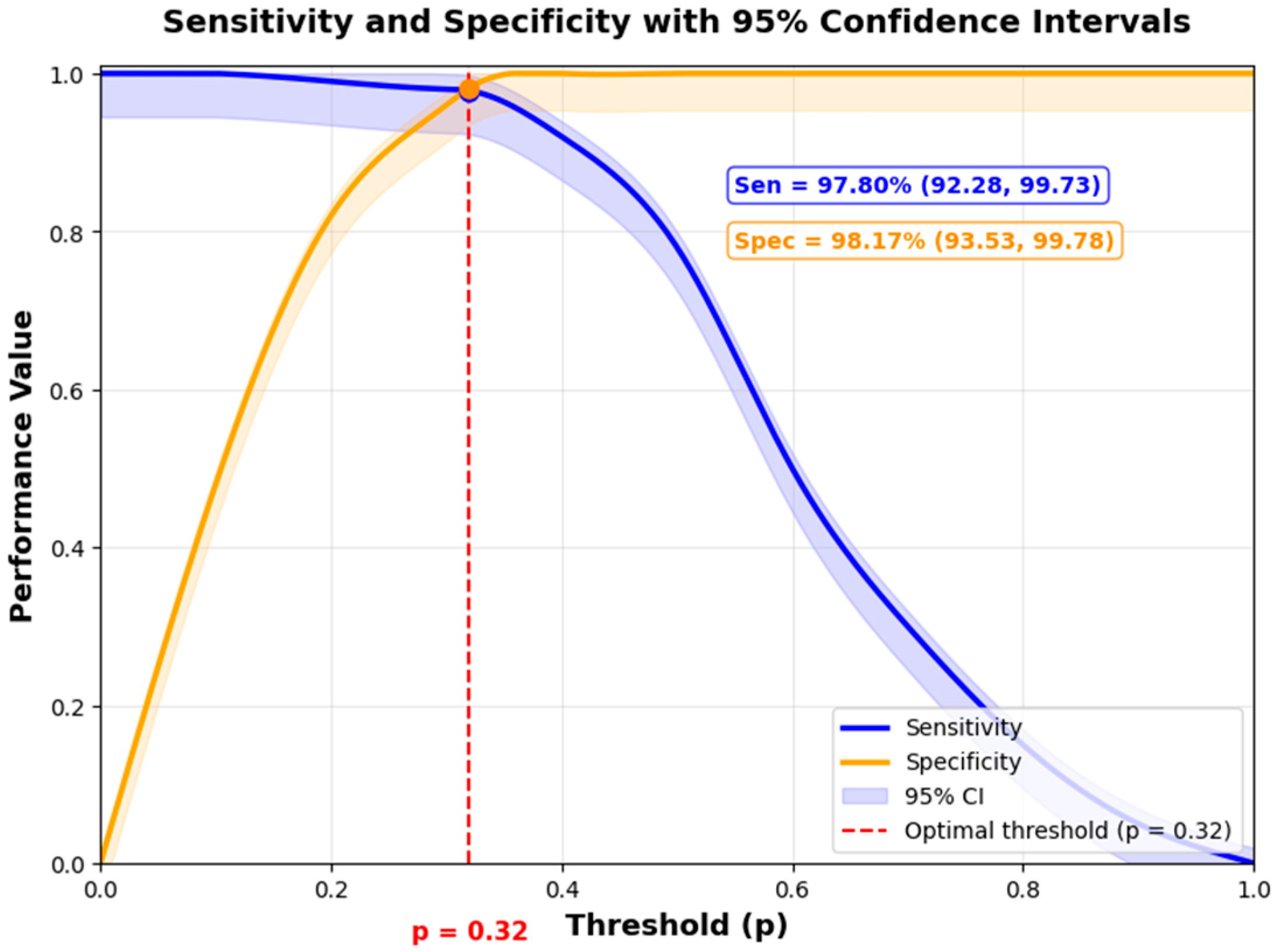
To identify the optimal classification threshold for HF prediction, we first performed a coarse search over the [0, 1] range in 0.05 increments, monitoring sensitivity and specificity to visualize the overall trade-off (Figure 7). The optimal threshold was then refined using a finer grid (step of 0.01) on the validation set, yielding a value of 0.32. This two-step procedure ensures both computational efficiency and precision. The resulting threshold was then fixed and applied to the independent test set to obtain the final performance metrics.
The curve illustrates the evolution of sensitivity (blue) and specificity (orange) as functions of the classification threshold. At low threshold values, sensitivity remains exceptionally high as nearly all patients are classified as positive, thereby maximizing the detection of true HF cases. Conversely, specificity is initially low due to numerous FP classifications of healthy patients. As the threshold increases, specificity improves reducing FP while sensitivity gradually declines as some TP cases are missing. The optimal balance between these competing metrics was identified at threshold p = 0.32 by maximizing Youden’s Index, representing the most favorable trade-off with sensitivity reaching 97.8 (92.28, 99.73) and specificity achieving 98.17 (93.53, 99.78). This equilibrium provides both exceptional TP detection and reliable negative classification, ensuring robust clinical utility. The outstanding performance at this threshold reflects the meta-learner’s superior capability to accurately detect and classify HF cases demonstrating its effectiveness in distinguishing pathological from healthy cardiac states with high precision and reliability.
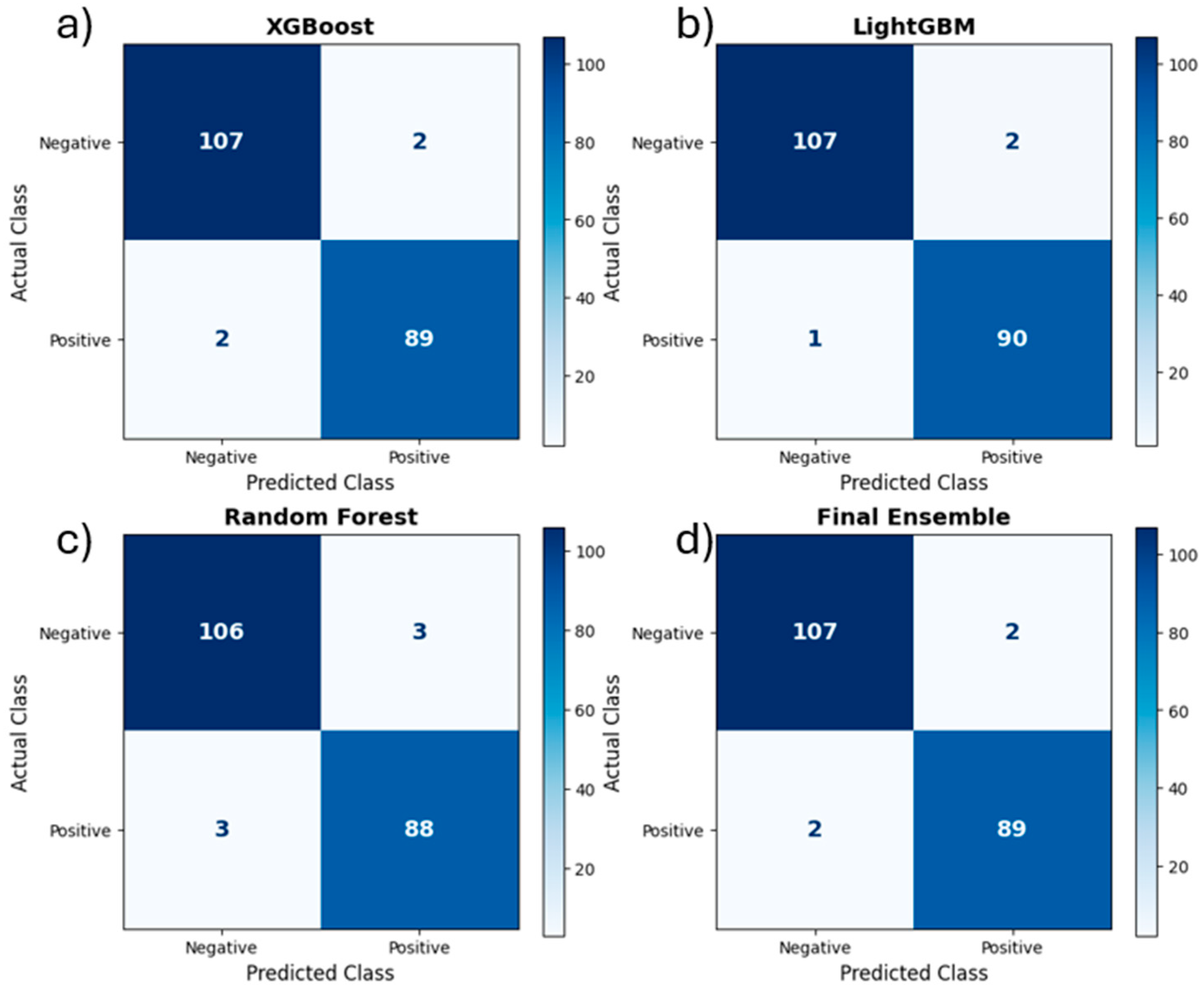
To provide a clinically transparent view of the model’s performance at the optimal threshold (p = 0.32), Figure 8a–d present the confusion matrices for the three individual meta-learners and the final ensemble model at the optimal threshold (p = 0.32). These matrices provide the number of correct and incorrect classifications, which is essential for evaluating the clinical impact of misclassifications, specifically missed diagnoses (false negatives) and unnecessary interventions (false positives).
XGBoost (Figure 8a) correctly identified 89 patients with HF (TP) and 107 patients without HF (TN), but missed 2 HF patients (FN). LightGBM (Figure 8b) showed the highest detection performance, with 90 TP and only 1 FN, corresponding to a sensitivity of 98.90%. Random Forest (Figure 8c) performed slightly lower with 88 TP and 3 FN, corresponding to a sensitivity of 96.70%. The final ensemble model (Figure 8d) achieved a balanced performance, with 89 TP, 2 FN, and only 2 FP. This means that 89 out of 91 HF patients were correctly detected while only 2 healthy patients were incorrectly classified as HF. This low false negative rate is clinically important, as missed diagnoses can lead to delayed treatment and worse outcomes.
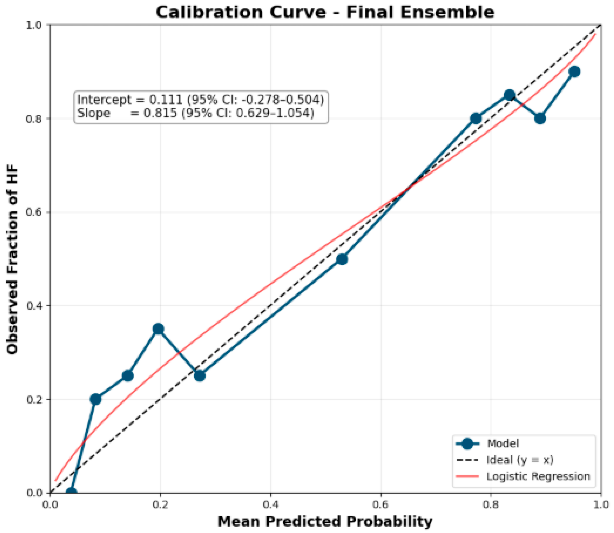
To assess the reliability of the probabilistic outputs, we evaluated the calibration of the final ensemble model. Figure 9 presents the calibration plot, comparing the predicted probabilities with the observed frequencies of heart failure.
Examination of the calibration plot in Figure 9 reveals a strong alignment with the ideal diagonal, indicating good concordance between the predicted probabilities and the observed event rates. The calibration intercept is 0.111 (95% CI: −0.278 to 0.504) and the slope is 0.815 (95% CI: 0.629 to 1.054). The intercept is close to zero, and its confidence interval encompasses zero, confirming the absence of significant systematic over- or under-estimation. Although the slope falls slightly below unity, the confidence interval includes 1, suggesting only a modest tendency to overestimate risks at lower probabilities and underestimate them at higher probabilities. Collectively, these findings support the reliability of the model’s calibration.
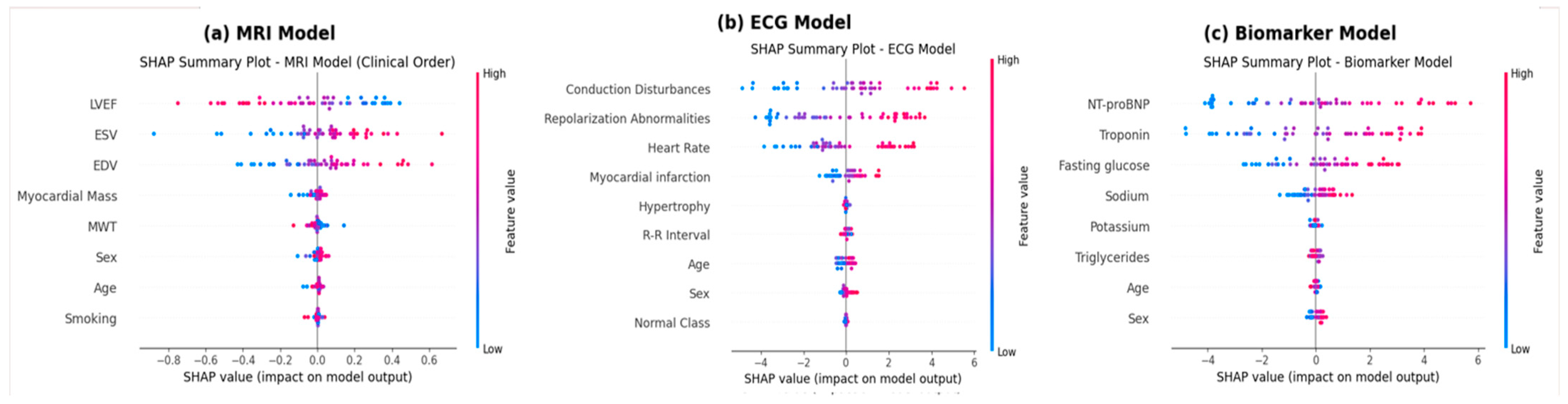
To further interpret the model’s decisions and quantify the contribution of individual features, we performed SHAP analyses for each modality-specific model. Figure 10 presents the SHAP summary plots for the MRI, ECG, and biomarker-based models.
The SHAP analysis for the MRI-based model (Figure 10a) shows that LVEF is the most influential feature, followed by ESV. Low LVEF values (blue) are associated with positive SHAP values, reflecting increased HF risk, while high LVEF values (red) are associated with negative SHAP values, indicating a protective effect. Similarly, high ESV values (red) are associated with positive SHAP values, consistent with its role as a marker of ventricular dysfunction. EDV, myocardial mass and MWT show moderate contributions, reflecting dilatation, hypertrophy and remodeling while age, smoking and sex have lower impacts, consistent with their roles as secondary risk factors.
Regarding the ECG-based model (Figure 10b), the SHAP analysis reveals that conduction disturbances are the most influential features, followed by repolarization abnormalities and heart rate. This hierarchy reflects the clinical importance of electrical remodeling, ventricular dyssynchrony and autonomic imbalance in HF. Myocardial infarction and hypertrophy also contribute significantly, consistent with their roles as structural and ischemic risk factors. Age and sex show lower contributions, consistent with their demographic nature, while the normal class has the lowest impact, reflecting its role as a control reference.
Regarding the biomarker-based model (Figure 10c), the SHAP analysis shows that NT-proBNP is the most influential feature, followed by troponin and fasting glucose. This hierarchy reflects the central role of neurohormonal activation, myocardial injury and metabolic dysregulation in HF. Sodium and potassium also contribute consistently with their roles in fluid balance and arrhythmic risk. Age and sex show lower contributions, consistent with their demographic nature. Overall, these results confirm that the model relies on clinically meaningful features across all modalities, reinforcing its interpretability.
To assess the robustness of the final ensemble model across different patient populations, we performed subgroup analyses by age (<60 vs. ≥60 years), HF severity (mild/moderate vs. severe), and comorbidity status (with vs. without at least one associated condition such as diabetes or hypertension, or renal disease). The results are reported in Table 14.
The model demonstrates strong and consistent performance across all subgroups, including older patients, severe HF cases, and those with comorbidities. While slight variations are observed, the framework remains highly effective across diverse patient populations, confirming its clinical robustness.
To provide a practical illustration of the model’s behavior, we examined three representative cases: a healthy subject, a patient with moderate HF, and a patient with severe decompensated HF. Table 15 reports their clinical characteristics, modality-specific predictions, and final ensemble risk scores.
The results show a clear gradient in risk scores that mirrors clinical severity. The healthy subject receives a low risk score of 0.08, while the moderate-HF patient scores 0.78, and the severe-HF patient scores 0.92.

5. Discussion

The present study investigates the feasibility of a late-fusion meta-learning framework for HF prediction that integrates complementary predictions derived from imaging, electrophysiological and biochemical modalities. This approach addresses a critical gap in current clinical practice by enabling comprehensive risk assessment even when some modalities are missing, thereby reflecting real-world diagnostic variability. To contextualize our findings, we conducted a comparative analysis with representative recent studies on heart failure prediction (Table 16).
Before discussing the comparative results, it is important to acknowledge that the studies summarized in this section were conducted using different datasets, patient populations, data modalities, and evaluation protocols. Consequently, direct quantitative comparisons should be interpreted with caution. The purpose of this comparison is not to establish a strict head-to-head ranking of methods but rather to position the proposed framework within the current body of heart failure prediction research. To the best of our knowledge, no previous study has evaluated a multimodal framework integrating cine-MRI, ECG, and biomarker data using the same experimental design adopted in this work. Therefore, the reported literature results serve primarily as contextual benchmarks that help illustrate the potential relevance and originality of the proposed approach. Despite these methodological differences, the comparison remains informative for highlighting current research trends, identifying existing limitations, and assessing the potential contribution of multimodal learning strategies for heart failure prediction.
The comparative analysis of recent studies reveals notable differences in dataset composition, input modalities, feature richness, and predictive performance. Several works leveraged large-scale databases such as MIMIC-IV [30,34] or the UK Biobank [35], while others relied on smaller institutional cohorts or self-constructed datasets [33,36]. From a feature engineering perspective, the number of features directly influences model complexity and interpretability. The studies compared in Table 16 employ feature sets ranging from 15 to 30 variables. Our framework uses 25 features, which places it between simpler configurations with fewer than ten features [31] and more complex models using up to 30 features [30]. This balanced choice captures a rich and clinically meaningful picture of HF pathophysiology, combining cine-MRI, ECG, biomarkers, and demographics. Consequently, this enables the framework to exploit complementary diagnostic information provided by different modalities, an aspect that is only partially addressed by unimodal or simpler bimodal approaches. The architecture of our framework was also designed to optimize performance and interpretability. Rather than training a single highly complex network, we designed modality-specific learners (Attention U-Net, MLP, XGBoost, LightGBM, and Random Forest), followed by a meta-learner fusion stage. This modular design enhances interpretability, reduces computational burden, and ensures that each modality contributes optimally to the final prediction, unlike previous studies that often rely on a single model for all features. This modular design is further leveraged by averaging the outputs of the three meta-learners. XGBoost and LightGBM are boosting-based algorithms, while Random Forest relies on bagging. Averaging their output balances their complementary biases. This approach reduces prediction variance and mitigates overfitting, while preserving strong discriminative performance.
Beyond the choice of meta-learners, the contribution of each modality-specific cohort was also assessed through cohort combination experiments. The MRI cohort achieves the highest individual accuracy (96.00%), reflecting its ability to capture detailed structural and functional cardiac information. The ECG cohort adds substantial value when combined with MRI, improving sensitivity by 1.6% (from 95.80% to 97.40%). This gain reflects its unique ability to detect early electrical abnormalities, such as arrhythmia or conduction defects, that may precede structural or biochemical changes. The biomarker cohort, although less sensitive in early stages, provides highly specific information, particularly in advanced HF, improving overall specificity when added to imaging and ECG and helping to reduce false positives. These findings confirm that predictions from each cohort are not redundant; each provides distinct and complementary information. Their combination yields the highest performance (98.00%), supporting the feasibility of integrating independently trained cohort-specific predictions within a unified decision-level framework. However, we acknowledge that these experiments compare cohort combinations rather than modalities within matched patients, reflecting the independent-cohort nature of our data and the cohort-pooling design of this feasibility study.
In terms of predictive performance, most recent studies report accuracies between 91% and 98% and AUC values up to 0.997 [34,36]. Our multimodal system achieved an accuracy of 98.00% (95% CI: 94.96–99.45), a sensitivity of 97.80% (95% CI: 92.28–99.73), a specificity of 98.17% (95% CI: 93.53–99.78), an F1-score of 97.80% (95% CI: 93.6–99.8), and an AUC of 0.978 (95% CI: 0.945–0.996).
These results demonstrate competitive performance relative to the state of the art, achieved despite a relatively smaller cohort, and match or surpass the best reported performances. Among the compared studies, Chen et al. [36] reported the highest accuracy (98.50%) and AUC (0.997) using a GCN-based model combining ECG and clinical text. Similarly, Teoh et al. [34] achieved an AUC of 0.996 using a late-fusion strategy combining tabular data, clinical notes, and chest X-rays. Ghazal [33] reported an accuracy of 95.70% and an AUC of 0.975 by fusing ECG, chest X-rays, biomarkers, and clinical text. Our framework, which integrates cine-MRI, ECG, biomarkers, and demographic data, offers a balanced performance across all metrics. Notably, our approach achieves the highest sensitivity (97.80%) among the compared studies, which is critical for minimizing missed diagnoses in clinical practice. It should also be emphasized that our work focuses on diagnostic prediction, identifying existing HF cases, rather than on prognostic forecasting of future outcomes or disease progression.”
Beyond overall performance, the clinical relevance of the model was reinforced by confusion matrix and calibration analyses. The final ensemble model showed a low false negative rate (2.2%), which is clinically critical to avoid missed diagnoses, and a low false-positive rate (1.8%), which limits unnecessary interventions. The calibration analysis further supported reliability, with an intercept close to zero and a slope whose confidence interval included 1, confirming the clinical acceptability of the predicted probabilities.
These results are supported by the diversity of the extracted features combined with modality-specific learners and a meta-learning late fusion strategy, representing a novel and effective contribution. By handling real-world data incompleteness and ensuring balanced sensitivity–specificity performance, our framework provides a clinically reliable and adaptable diagnostic tool. Such an approach holds promise for personalized risk assessment, early intervention and improved patient outcomes. Unlike early feature fusion, which requires aligned multimodal data and is highly sensitive to missing inputs, our late-fusion design was specifically chosen to operate under the constraints of retrospective clinical data, where patient-level alignment is rarely feasible, as detailed in Section 3.5.4.
Despite its strengths, this study has several limitations. First, the retrospective nature of the data and the integration of heterogeneous datasets collected across different institutions and populations introduce variability in acquisition protocols and measurement conditions. Such heterogeneity may lead to distribution shifts across modalities, potentially affecting model robustness and generalization.
Second, the absence of patient-level alignment across all modalities and the lack of external validation on independent cohorts limit the interpretability of absolute performance metrics and may result in optimistic performance estimates when evaluated within the same experimental setting. This risk is further compounded by the heterogeneity of the original datasets—collected from different institutions, populations, and protocols—which may introduce cohort-specific biases despite the mitigating effect of our late-fusion design. Nevertheless, the reported results should be interpreted as a methodological benchmark established under controlled experimental conditions, providing a solid reference for future large-scale and externally validated studies.
Third, despite the strict separation of training and test sets and late fusion strategy, we acknowledge a theoretical concern regarding label leakage, as variables used to define HF are also included as predictors.
Finally, the current framework focuses on heart failure prediction at a single time point and does not model longitudinal disease progression. Extending the framework to incorporate temporal dynamics and external cohorts represents a promising direction for future work, enabling improved long-term monitoring and prognostic assessment. In addition, we did not perform a formal decision curve analysis (DCA), as this analysis requires clinically meaningful risk thresholds and explicit weighting of treatment benefits and harms. This remains an important perspective for future research.

6. Conclusions

This study demonstrates the potential of a multimodal late-fusion framework integrating complementary information derived from cine-MRI, ECG, biomarker, and demographic data for accurate heart failure prediction. By employing modality-specific models trained on pre-extracted features, our framework reduced computational complexity while maintaining competitive predictive performance. With an accuracy of 98.00% (95% CI: 94.96–99.45), sensitivity of 97.8% (95% CI: 92.28–99.73), specificity of 98.17% (95% CI: 93.53–99.78), F1-score of 97.8% (95% CI: 93.6–99.8), and AUC of 0.978 (95% CI: 0.945–0.996), the framework demonstrates that the proposed late-fusion strategy effectively leverages complementary imaging, physiological, and clinical information for robust predictive modeling. To the best of our knowledge, this is the first framework to combine independently developed cine-MRI, ECG, and biomarker prediction models within a unified decision-level framework for HF prediction. The results, supported by favorable calibration and low false negative rates, demonstrate the feasibility of integrating cohort-specific predictions within a unified decision-level framework.

Supplementary Materials

The following supporting information can be downloaded at: https://www.mdpi.com/article/10.3390/technologies14080496/s1.

Author Contributions

Conceptualization: W.B., Methodology: W.B., N.B. and S.L.; Software: W.B., Validation: W.B., S.L., N.B. and A.A.A.; Formal analysis: W.B., A.A.A. and Z.A.; Investigation: W.B.; Resources: W.B., A.K., Z.A. and A.A.A.; Data curation: W.B. and A.K., Writing—original draft: W.B.; Writing—review & editing: W.B., S.L. and N.B.; Visualization: W.B.; Supervision: S.L. and A.J.; Project administration: S.L., A.J. and A.K. All authors have read and agreed to the published version of the manuscript.

Funding

This research received no external funding.

Institutional Review Board Statement

The authors affirm that all procedures involving human participants in this study were conducted in strict accordance with the ethical standards of the institutional research committee, as well as the principles outlined in the 1964 Declaration of Helsinki and its subsequent amendments or equivalent ethical guidelines. As the nature of this study is purely observational and involves retrospective data analysis, formal informed consent was not required. No names, identifiers, or personal information were used; the dataset exclusively comprised anonymized information related to heart failure. Moreover, the researchers had no access to any identifying details or professional background of the patients, except for their age, sex and diagnosed condition.

Informed Consent Statement

Not applicable.

Data Availability Statement

Data are contained within the article. The analytical code is available upon reasonable request from the corresponding author.

Acknowledgments

The authors wish to express their sincere appreciation to the MRI Department at the Military Hospital of Tunis and to the Biochemistry Laboratory team at La Rabta Hospital for their valuable collaboration. Their assistance in providing anonymized datasets ensured full respect for patient confidentiality and allowed comprehensive analyses to be conducted on both healthy individuals and patients with heart failure. The Researchers would like to thank the Deanship of Graduate Studies and Scientific Research at Qassim University for financial (QU-APC) support (السنة الميلادية). The authors acknowledge the use of AI-assisted language editing tools to improve the English language and readability of the manuscript. All scientific content, analyses, and conclusions were produced by the authors.

Conflicts of Interest

The authors declare no conflicts of interest.

Abbreviations

The following abbreviations are used in this manuscript:
AIArtificial Intelligence
AUC-ROCArea Under the Receiver Operating Characteristic Curve
CNNConvolutional Neural Network
DNNDeep Neural Network
ECGElectrocardiogram
EDVEnd-Diastolic Volume
ESVEnd-Systolic Volume
HFHeart Failure
LVLeft Ventricle
LVEFLeft Ventricular Ejection Fraction
LVHLeft Ventricular Hypertrophy
MIMyocardial Infarction
MLMachine Learning
MLPMultilayer Perceptron
MSEMean Squared Error
MWTMyocardial Wall Thickness
RFRandom Forest
SVMSupport Vector Machine
XGBoostExtreme Gradient Boosting

References

  1. Chen, S.; Huang, Z.; Liang, Y.; Zhao, X.; Aobuliksimu, X.; Wang, B.; He, Y.; Kang, Y.; Huang, H.; Li, Q.; et al. Five-year mortality of heart failure with preserved, mildly reduced, and reduced ejection fraction in a 4880 Chinese cohort. ESC Heart Fail. 2022, 9, 2336–2347. [Google Scholar] [CrossRef] [PubMed]
  2. Khan, M.S.; Shahid, I.; Bennis, A.; Rakisheva, A.; Metra, M.; Butler, J. Global epidemiology of heart failure. Nat. Rev. Cardiol. 2024, 21, 717–734. [Google Scholar] [CrossRef] [PubMed]
  3. Savarese, G.; Moritz, P.; Becher, P.M.; Lund, L.H.; Seferovic, P.; Rosano, G.M.C.; Coats, A.J.S. Global burden of heart failure: A comprehensive and updated review of epidemiology. Cardiovasc. Res. 2022, 118, 3272–3287. [Google Scholar] [CrossRef] [PubMed]
  4. Medhi, D.; Kamidi, S.R.; Sree, K.P.M.; Shaikh, S.; Rasheed, S.; Murichathil, A.H.T.; Nazir, Z. Artificial intelligence and its role in diagnosing heart failure: A narrative review. Cureus 2024, 16, e59661. [Google Scholar] [CrossRef] [PubMed]
  5. Adnan, M.; Yi, Y.; Wang, E.; Imtiaz, M.N. StackTrans—Multimodal Heart Disease Detection Using Stacked Transformer Fusion Framework. IEEE Access 2025, 13, 99911–99922. [Google Scholar] [CrossRef]
  6. Sangha, V.; Nargesi, A.A.; Dhingra, L.S.; Khunte, A.; Mortazavi, B.J.; Ribeiro, A.H.; Banina, E.; Adeola, O.; Garg, N.; Brandt, C.A.; et al. Detection of left ventricular systolic dysfunction from electrocardiographic images. Circulation 2023, 148, 765–777. [Google Scholar] [CrossRef] [PubMed]
  7. Awadi, R.; Benameur, N.; Hafsi, H.; Younes, T.B.; Arous, Y.; Labidi, S.; Tavares, J.M.R. Myocardial Strain Assessment for Early Duchenne Muscular Dystrophy Diagnosis in Pediatric Patients Using Cardiac MRI. Appl. Sci. 2024, 14, 10341. [Google Scholar] [CrossRef]
  8. Singh, M.S.; Thongam, K.; Choudhary, P.; Bhagat, P.K. An integrated machine learning approach for congestive heart failure prediction. Diagnostics 2024, 14, 736. [Google Scholar] [CrossRef] [PubMed]
  9. Moshawrab, M.; Adda, M.; Bouzouane, A.; Ibrahim, H.; Raad, A. Cardiovascular events prediction using artificial intelligence models and heart rate variability. Procedia Comput. Sci. 2022, 203, 231–238. [Google Scholar] [CrossRef]
  10. Kottapalle, P.; Tak, T.K.; Kshirsagar, P.R.; Ginnela, G.; Akula, V.K. QHF-CS: Quantum-Enhanced Heart Failure Prediction Using Quantum CNN with Optimized Feature Qubit Selection with Cuckoo Search in Skewed Clinical Data. Comput. Mater. Contin. 2025, 84, 3857–3892. [Google Scholar] [CrossRef]
  11. Wang, J.; Xue, Q.; Zhang, C.W.J.; Wong, K.K.L.; Liu, Z. Explainable coronary artery disease prediction model based on AutoGluon from AutoML framework. Front. Cardiovasc. Med. 2024, 11, 1360548. [Google Scholar] [CrossRef] [PubMed]
  12. Gao, Y.; Jiang, Y.; Peng, Y.; Yuan, F.; Zhang, X.; Wang, J. Medical Image Segmentation: A Comprehensive Review of Deep Learning-Based Methods. Tomography 2025, 11, 52. [Google Scholar] [CrossRef] [PubMed]
  13. Kumar, D.; Balraj, K.; Seth, S.; Vashista, S.; Ramteke, M.; Rathore, A.S. An improved machine learning-based prediction framework for early detection of events in heart failure patients using mHealth. Health Technol. 2024, 14, 495–512. [Google Scholar] [CrossRef]
  14. Panchal, R.; Tiwari, S.; Agarwal, S. Multimodal image fusion on ECG signals for congestive heart failure classification. Multimed. Tools Appl. 2025, 84, 8247–8259. [Google Scholar] [CrossRef]
  15. Khan, S.; Khan, A.A.; Mahendran, R.K.; Fazil, M.; Rehman, A.U.; Jiang, W.; Farouk, A. C2DEEP-OT: Utilizing Multi-Agent Deep Reinforcement Learning Algorithm and Optimized Attentive Transformer Network for Cervical Cancer Detection. Inf. Sci. 2025, 738, 123047. [Google Scholar] [CrossRef]
  16. Chandraman, M.; Santhiyakumari, N.; Shree, K.V.M.; Murugesan, M.; Kumarganesh, S.; Rishabavarthani, P.; Sahani, S.K. Enhancing Cardiovascular Disease Analysis in Healthcare Systems with Hybrid Random Forest and Neural Network Algorithm. Eng. Rep. 2025, 7, e70373. [Google Scholar] [CrossRef]
  17. Lin, C.H.; Liu, Z.Y.; Chu, P.H.; Chen, J.S.; Wu, H.H.; Wen, M.S.; Kuo, C.F.; Chang, T.Y. A multitask deep learning model utilizing electrocardiograms for major cardiovascular adverse events prediction. npj Digit. Med. 2025, 8, 1. [Google Scholar] [CrossRef] [PubMed]
  18. Zhang, Z.; Li, D.; Zhao, J.; Ma, H.; Wang, F.; Hao, Q. Heart failure prognosis risk assessment model based on multimodal data fusion and IoT device monitoring. Alex. Eng. J. 2025, 127, 722–732. [Google Scholar] [CrossRef]
  19. Punn, N.S.; Dewangan, D.K. Ensemble Meta-Learning using SVM for Improving Cardiovascular Disease Risk Prediction. medRxiv 2024, 125, 1–15. [Google Scholar] [CrossRef]
  20. Wagner, P.; Strodthoff, N.; Bousseljot, R.D.; Kreiseler, D.; Lunze, F.I.; Samek, W.; Schaeffter, T. PTB-XL, a large publicly available electrocardiography dataset. Sci. Data 2020, 7, 1–15. [Google Scholar] [CrossRef]
  21. Ronneberger, O.; Fischer, P.; Brox, T. U-net: Convolutional networks for biomedical image segmentation. In Proceedings of the International Conference on Medical Image Computing and Computer-Assisted Intervention; Springer International Publishing: Cham, Switzerland, 2015; pp. 234–241. [Google Scholar] [CrossRef]
  22. Baccouch, W.; Oueslati, S.; Solaiman, B.; Lahidheb, D.; Labidi, S. Automatic left ventricle volume and mass quantification from 2D cine-MRI: Investigating papillary muscle influence. Med. Eng. Phys. 2024, 127, 104162. [Google Scholar] [CrossRef] [PubMed]
  23. Sinsomboonthong, S. Performance comparison of new adjusted min-max with decimal scaling and statistical column normalization methods for artificial neural network classification. Int. J. Math. Math. Sci. 2022, 2022, 3584406. [Google Scholar] [CrossRef]
  24. Paul, A.; Bandyopadhyay, R.; Yoon, J.H.; Geem, Z.W.; Sarkar, R. SinLU: Sinu-sigmoidal linear unit. Mathematics 2022, 10, 337. [Google Scholar] [CrossRef]
  25. Wiens, M.; Verone-Boyle, A.; Henscheid, N.; Podichetty, J.T.; Burton, J. A tutorial and use case example of the eXtreme gradient boosting (XGBoost) artificial intelligence algorithm for drug development applications. Clin. Transl. Sci. 2025, 18, e70172. [Google Scholar] [CrossRef] [PubMed]
  26. Chai, X.; Li, J.; Zhao, J.; Wang, W.; Zhao, X. LGB-PHY: An evaporation duct height prediction model based on physically constrained lightGBM algorithm. Remote Sens. 2022, 14, 3448. [Google Scholar] [CrossRef]
  27. Fatima, S.; Hussain, A.; Amir, S.B.; Ahmed, S.H.; Aslam, S.M.H. Xgboost and random forest algorithms: An in depth analysis. Pak. J. Sci. Res. 2023, 3, 26–31. [Google Scholar] [CrossRef]
  28. Liao, H.; Zhang, X.; Zhao, C.; Chen, Y.; Zeng, X.; Li, H. LightGBM: An efficient and accurate method for predicting pregnancy diseases. J. Obstet. Gynaecol. 2022, 42, 620–629. [Google Scholar] [CrossRef] [PubMed]
  29. Baccouch, W.; Hasnaoui, B.; Benameur, N.; Jemai, A.; Lahidheb, D.; Labidi, S. Deep Learning-Based Algorithm for the Classification of Left Ventricle Segments by Hypertrophy Severity. J. Imaging 2025, 11, 244. [Google Scholar] [CrossRef] [PubMed]
  30. Botros, J.; Mourad-Chehade, F.; Laplanche, D. Explainable multimodal data fusion framework for heart failure detection: Integrating CNN and XGBoost. Biomed. Signal Process. Control 2025, 100, 106997. [Google Scholar] [CrossRef]
  31. Liang, X.; Jiang, N.; Qi, P.; Chen, Z.; Tong, J.; Xia, S. ECGEL: A multimodal 12-lead ECG classification model for heart failure prediction. Biomed. Eng. Lett. 2025, 15, 537–547. [Google Scholar] [CrossRef] [PubMed]
  32. Liu, J.; Zhu, D.; Deng, L.; Chen, X. Predictive Modeling of Heart Failure Outcomes Using ECG Monitoring Indicators and Machine Learning. Ann. Noninvasive Electrocardiol. 2025, 30, e70097. [Google Scholar] [CrossRef] [PubMed]
  33. Ghazal, M.T. Multimodal fusion framework for enhanced diagnosis of heart failure using ECG, chest X-rays, blood biomarkers, and clinical text data. Iran J. Comput. Sci. 2026, 9, 42. [Google Scholar] [CrossRef]
  34. Teoh, J.R.; Hasikin, K.; Wong, H.D.; Ng, W.L.; Lee, K.W.; Kiew, L.V.; Lai, K.W. Multimodal late fusion for heart failure diagnosis using tabular and chest X-ray data: A comparative study of fusion strategies. Biomed. Signal Process. Control. 2026, 120, 110106. [Google Scholar] [CrossRef]
  35. Peng, J.; Beetz, M.; Banerjee, A.; Chen, M.; Grau, V. AEM: An interpretable multi-task multi-modal framework for cardiac disease prediction. Med. Image Anal. 2026, 109, 103951. [Google Scholar] [CrossRef] [PubMed]
  36. Chen, Y.; Liang, X.; Qi, P.; Xia, S.; Tong, J. Multimodal heart failure prediction model based on graph convolutional neural network. Biomed. Eng. Lett. 2026, 1–10. [Google Scholar] [CrossRef]
Figure 1. Overview of Proposed Framework for Heart Failure Prediction.
Technologies 14 00496 g001
Figure 2. Overall architecture of Attention U-Net proposed for left ventricle contour extraction.
Technologies 14 00496 g002
Figure 3. Feature values for 10 representative patients before (left) and after (right) normalization.
Technologies 14 00496 g003
Figure 4. MLP architecture for heart failure probability prediction from cine-MRI features.
Technologies 14 00496 g004
Figure 5. A representative sample of 10 patients showing the original feature values (left) and the processed feature set (right) after preprocessing for model input.
Technologies 14 00496 g005
Figure 6. Feature values for a sample of 10 patients before (a) and after (b) preparation.
Technologies 14 00496 g006
Figure 7. Sensitivity and specificity evolution across classification thresholds with 95% confidence intervals (shaded areas). The red dashed line marks the optimal threshold (p = 0.32) determined by Youden’s index. The corresponding sensitivity and specificity values at this threshold are reported in the inset.
Technologies 14 00496 g007
Figure 8. Confusion matrices at the optimal threshold (p = 0.32) for (a) XGBoost, (b) LightGBM, (c) Random Forest, and (d) the final ensemble model.
Technologies 14 00496 g008
Figure 9. The calibration plot for the final ensemble model. The blue curve represents observed vs. predicted probabilities, the red dashed line shows the logistic regression fit, and the black dashed line corresponds to the ideal calibration (y = x). Intercept and slope values are provided in the inset.
Technologies 14 00496 g009
Figure 10. SHAP summary plots for the (a) MRI, (b) ECG, and (c) biomarker models. Red: high feature values; blue: low feature values. Positive SHAP values increase HF risk; negative values decrease it.
Technologies 14 00496 g010
Table 1. Summary of AI-driven heart failure prediction studies.
Ref.YearHeart DiseaseDatabase/ModalityFeature CountAI-ModelPerformance MeasuresChallenges
[8]2024Heart Failure5888 participants/clinical, demographic features + lifestyle factors + laboratory results12LR, Random forest, SVM, naive Bayes decision tree, DNNAcc = 95.30%
F1-score = 97.03%,
Sen = 96.49%, Pre = 97.58%
Reliance on a single dataset without external validation limits generalizability
[9]2024Heart failureThree public datasets: UCI heart disease, Framingham, Faisalabad/ECG, angiography13a new guided attentive HF prediction approachAcc = 98%Single-center origin and absence of external validation may restrict generalizability; feature ranking remains complex
[11]2024Coronary artery diseaseFive public datasets: Cleveland, Hungary, Switzerland, VA Long Beach and Statlog12AutoGluon modelAUC = 95.62
Acc = 91.67
Group imbalance, no propensity matching, unclear case timing, and missing confounder data limit model validity.
[13]2024Heart failure128 patients/biological, ECG demographic33Gaussian Naive Bayes, SVM, MLPCPre = 98%
Re = 91%
F1-score = 0.94%
Dependence on extensive hyperparameter tuning
[19]2024Cardiovascular disease70,000 samples/ECG, imaging, demographic features, clinical features11Meta-learning using SVMAcc = 90% Auc-ROC = 94%
Pre = 87%
Re = 88%, F1-score = 87%
Careful feature engineering, guided by domain knowledge, is crucial for maximizing performance.
[10]2025Heart failure299 medical records, Cleveland, Hungarian, Switzerland, Long Beach, VA, and Statlog databases13Enhanced Quantum CNNAcc = 94%
pre = 94%
Re = 95% F1-score = 94%
Absence of real-time predictive capability and lack of validation on actual quantum hardware.
[14]2025Heart failure5000 ECG recordings/Multimodal Feature Fusion-Convolutional Neural Networks (CNNs) and Gated Recurrent Units (GRUs)Acc = 97.79% for MIF and 98.19% for MFFDependence on high-quality ECG signal preprocessing and the absence of external validation limit generalizability
[17]2025Cardiac disease2,821,889 standard 12-lead ECGs12Deep neural networkAUROCs of 0.90 for heart failure (HF)High dimensionality of raw ECG data increases computational complexity and may hinder model interpretability
[18]2025Heart failureEMR dataset/Chest X-ray image dataset-CNN + graph neural networksAcc = 97.2%
ROC (AUC) = 97.2%,
High complexity and limited external validation
Table 2. Description of Cine-MRI Features.
FeatureDescriptionTypical ValuesClinical Relevance for HF Prediction
LVEFPercentage of left ventricular blood volume ejected during systole (%)55–70%Reduced LVEF is a direct marker of systolic HF
EDVLeft ventricular volume measured at the end of diastole (mL)120–210 mLElevated EDV indicates ventricular dilatation, common in HF with reduced EF
ESVLeft ventricular volume measured at the end of systole (mL)50–80 mLElevated ESV reflects impaired contraction, predicting systolic dysfunction
MWTAverage thickness of LV myocardium (mm)6–15 mmIncreased thickness suggests hypertrophy; decreased thickness may indicate remodeling or atrophy
Myocardial massTotal mass of LV myocardium (g)100–200 gElevated mass reflects hypertrophy and structural remodeling linked to HF
Table 3. Diagnostic features extracted from the ECG database.
FeaturesDescriptionTypical ValuesClinical Relevance
Myocardial infarction (MI)Presence of prior myocardial infarction, based on ECG annotationBinary
(Yes = 1, No = 0)
Previous MI leads to myocardial damage and is a major risk factor for heart failure
Conduction Disturbances (CDs)Abnormalities in impulse conduction such as bundle branch block or atrioventricular blockBinary
(Yes = 1, No = 0)
Conduction abnormalities impair ventricular synchronization and contribute to reduced cardiac function.
HypertrophyEvidence of ventricular hypertrophy from ECG patternsBinary
(Yes = 1, No = 0)
Hypertrophy increases myocardial workload and predisposes to heart failure.
Repolarization AbnormalitiesAlterations in ST segment or T-waveBinary
(Yes = 1, No = 0)
ST-segment deviations and T-wave abnormalities indicate ventricular electrical instability, reflecting underlying ischemia or ventricular stress.
Normal Class (NORM)Absence of pathological findings in the ECGBinary
(Yes = 1, No = 0)
Serves as a control reference for distinguishing healthy from pathological signals.
R–R IntervalServes as a control reference for distinguishing healthy from pathological signals.~600–1200 ms (normal sinus rhythm: 50–100 bpm)Reflects heart rate variability; deviations may indicate arrhythmias or autonomic imbalance in heart failure.
Heart RateNumber of heart beats per minute derived from R–R intervals~50–100 bpmProvides a direct measure of cardiac function; tachycardia or bradycardia can signal HF risk.
Table 4. Description of Biochemical Features in Biological Dataset.
FeatureDescriptionTypical Values or NormsClinical Relevance
TroponinCardiac-specific biomarker indicating myocardial injury<0.04 ng/mLMarker of ongoing myocardial damage
NT-proBNPBiomarker of ventricular wall stress and overload<125 pg/mLIndicator of heart failure severity
Fasting glucoseBlood glucose after overnight fast70–100 mg/dLMetabolic risk factor
TriglyceridesBlood lipid measurement<150 mg/dLDyslipidemia, cardiovascular risk
SodiumSerum sodium concentration135–145 mmol/LElectrolyte balance
PotassiumSerum potassium concentration3.5–5.0 mmol/LElectrolyte and cardiac electrophysiology
Table 5. Performance of Attention U-Net under different hyperparameter configurations.
ParametersEpochsBatch Size = 4Batch Size = 8
AdamAdamaxAdamAdamax
Learning
Rate
10−22065.2267.6466.1868.06
4071.0672.1171.0573.55
6073.4575.8174.4476.37
8075.3477.1376.6778.64
10−32078.1581.1279.2382.54
4084.4186.3285.3588.31
6088.3691.1089.7893.67
8091.3394.0892.9397.25
10−42070.7371.5472.1173.43
4073.6676.2677.5678.27
6079.0980.7281.9082.28
8082.5184.6785.6586.56
Table 6. Quantitative endocardial and epicardial segmentation results for a healthy subject and a patient with HF using the proposed Attention U-Net.
Patient/SectionMean HD (mm)Mean DSC (%)
EndoEpiEndoEpi
Healthy patientBasal section7.342 ± 2.46.421 ± 2.495.26 ± 3.198.76 ± 3.1
Mid-section6.832 ± 1.35.212 ± 3.196.41 ± 3.597.35 ± 2.0
Apical section7.154 ± 3.27.667 ± 0.394.17 ± 1.795.42 ± 4.2
Patient with heart failureBasal section8.174 ± 1.55.256 ± 1.795.24 ± 2.396.56 ± 3.4
Mid-section6.321 ± 1.16.778 ± 1.297.24 ± 1.198.01 ± 2.2
Apical section8.012 ± 0.27.022 ± 2.695.83 ± 2.396.17 ± 4.5
Table 7. MSE across hyperparameter configurations for the MLP model.
DepthLREpochsBatch Size = 8Batch Size = 16
AdamAdamaxRmspropAdamAdamaxRmsprop
2 hidden layers10−3700.0840.0800.0890.0920.0880.094
800.0800.0760.0850.0900.0860.091
900.0780.0740.0830.0910.0870.092
1000.0760.0720.0810.0930.0890.094
1200.0770.0730.0820.0950.0910.096
10−2700.0720.0680.0790.0880.0840.090
800.0680.0640.0760.0870.0830.089
900.0650.0610.0730.0880.0840.091
1000.0630.0590.0710.0900.0860.092
1200.0640.0600.0720.0910.0880.094
10−1700.0850.0810.0900.0940.0900.096
800.0830.0790.0880.0950.0910.097
900.0810.0770.0860.0960.0930.099
1000.0790.0750.0840.0990.0950.101
1200.0800.0760.0850.1010.0970.103
3 hidden layers10−3700.0880.0840.0930.0950.0910.096
800.0860.0820.0910.0970.0930.099
900.0840.0800.0890.1000.0950.100
1000.0830.0790.0880.1010.0970.103
1200.0840.0800.0890.1130.0990.105
10−2700.0800.0760.0850.0920.0880.094
800.0780.0740.0830.0930.0900.097
900.0760.0720.0810.0960.0920.098
1000.0750.0710.0800.0970.0940.100
1200.0760.0720.0810.1100.0960.102
10−1700.0900.0860.0950.0970.0930.099
800.0880.0840.0930.0990.0950.101
900.0870.0830.0910.1110.0970.123
1000.0860.0820.0900.1030.0990.106
1200.0870.0830.0910.1050.1010.107
Table 8. Representative Predicted Probabilities of Heart Failure Risk Before and After Platt Calibration.
PatientsProbabilities of Heart Failure Risk
Before CalibrationAfter Calibration
Patient 10.720.68
Patient 20.540.51
Patient 30.360.40
Patient 40.830.79
Table 9. Hyperparameter tuning results and selected values for the ECG-based XGBoost model.
ParameterTested ValuesOptimal Selected ValueJustification
n_estimators50, 100, 150100Balanced trade-off between performance and computational cost, reduces overfitting risk
max-depth3, 4, 54Moderate depth captures feature interactions without overfitting
learning rate0.01, 0.1, 0.20.1Provides a good balance between convergence speed and stability
Subsample0.6, 0.8, 1.00.8Ensures robustness while retaining most of the training samples
colsample_bytree0.6, 0.8, 1.00.8Maintains feature diversity per tree without losing important information
reg_alpha0, 0.1, 1.00.1Light L1 regularization to reduce overfitting risk
reg_lambda1, 1.5, 2.01.5Moderate L2 regularization improves model stability
min_child_weight1, 3, 51Allows the model to be sensitive to small but relevant signal variations
gamma0, 0.1, 2.00.1Adds light regularization to prevent overly specific splits
scale_pos_weight1, 1.5, 2.01No major class imbalance observed, hence no additional weighting needed
Table 10. Optimal hyperparameter configuration of XGBoost model for biomarker-based heart failure probability prediction.
ParameterTested ValuesOptimal Selected ValueJustification
n_estimators50, 80, 10080Balanced number of trees to capture variability without overfitting given the smaller dataset.
max-depth2, 3, 43Shallow trees prevent overfitting and ensure stable learning on limited biomarker data
learning rate0.01, 0.05, 0.10.05A moderately small learning rate stabilizes convergence while retaining efficiency.
Subsample0.6, 0.8, 1.01.0All samples are used since the cohort size (157 patients) is relatively small.
colsample_bytree0.6, 0.8, 1.01.0All features are included per tree, reflecting their strong and independent clinical significance.
reg_alpha0, 0.1, 1.00.1Mild L1 regularization improves generalization without discarding important biomarkers.
reg_lambda1.0, 1.5, 2.02.0Stronger L2 regularization reduces variance and enhances stability.
min_child_weight1, 3, 51Allows the model to split on fewer samples, capturing fine-grained patterns in biomarker variation.
gamma0, 0.1, 0.20.1Prevents overly complex splits while still allowing useful partitioning.
scale_pos_weight0.5, 0.67, 1.00.67Adjusted to compensate for class imbalance between HF and healthy groups
Table 11. Hyperparameter configurations tested and selected for XGBoost, Random Forest, and LightGBM meta-learners.
ParameterXGBoostRandom ForestLightGBM
Tested ValuesSelected ValueTested ValuesSelected ValueTested ValuesSelected Value
n_estimators50, 100, 15010050, 100, 20010050, 100, 200100
max_depth3, 4, 543, 5, 753, 4, 64
learning_rate0.01, 0.1, 0.20.1--0.01, 0.05, 0.10.05
Subsample/bagging fraction0.6, 0.8, 1.00.8--0.6, 0.8, 1.00.8
colsample/feature_fraction0.6, 0.8, 1.00.80.6, 0.8, 1.00.80.6, 0.8, 1.00.8
reg_alpha0, 0.1, 1.00.1--0, 0.1, 1.00.1
reg_lambda1, 1.5, 2.01.5--1, 1.5, 2.01.0
min_child_weight1, 3, 51--1, 2, 42
min_samples_split--2, 4, 62--
Table 12. Performance comparison of individual meta-learners and final ensemble model for heart failure prediction.
Metric XGBoostLightGBMRandom ForestFinal Ensemble (Meta-Learning)
MSE0.020 (0.013, 0.027)0.018 (0.011, 0.025)0.025 (0.018, 0.032)0.019 (0.013, 0.027)
Log-Loss0.065 (0.053, 0.077)0.060 (0.048, 0.072)0.075 (0.062, 0.088)0.063 (0.043, 0.081)
Brier Score0.014 (0.011, 0.017)0.012 (0.009, 0.015)0.016 (0.013, 0.019)0.013 (0.009, 0.021)
AUC-ROC0.975 (0.958, 0.992)0.981 (0.964, 0.998)0.968 (0.951, 0.985)0.978 (0.945, 0.996)
Accuracy (%)98.00 (94.96, 99.45)98.50 (95.68, 99.69)97.00 (93.6, 98.9)98.00 (94.96, 99.45)
Sensitivity (%)97.80 (92.28, 99.73)98.90 (94.03, 99.97)96.70 (90.7, 99.3)97.80 (92.28, 99.73)
Specificity (%)98.17 (93.53, 99.78)98.17 (93.53, 99.78)97.25 (92.17, 99.43)98.17 (93.53, 99.78)
F1-score (%)97.80 (92.0, 99.7)98.36 (94.0, 99.7)96.70 (92.1, 99.5)97.80 (93.6, 99.8)
PPV (%)97.80 (92.28, 99.7)97.83 (92.36, 99.73)96.70 (90.7, 99.31)97.80 (92.28, 99.73)
NPV (%)98.17 (93.53, 99.78)99.07 (94.95, 99.97)97.25 (92.17, 99.43)98.17 (93.53, 99.78)
Table 13. The performance of the final ensemble model across different cohort combinations (MRI only, ECG only, biomarkers only, and their combinations). Values are presented as estimates (95% confidence interval).
ModalitiesAccuracy (%)AUCSensitivity (%)Specificity (%)F1-Score (%)
MRI only96.00 (93.8, 97.8)0.962 (0.94–0.98)95.80 (92.1, 98.1)96.20 (93.8, 98.0)96.00 (93.0, 98.1)
ECG only94.50 (91.9, 96.5)0.948 (0.93–0.97)94.20 (91.1, 96.5)94.80 (91.9, 97.0)94.50 (91.0, 97.0)
Biomarkers only91.00 (88.1, 93.4)0.918 (0.89–0.94)91.00 (87.8, 93.8)91.00 (87.4, 93.9)91.00 (87.4, 93.9)
MRI + ECG97.50 (95.8, 98.7)0.975 (0.96–0.99)97.40 (92.5, 99.5)97.60 (93.0, 99.0)97.50 (93.0, 99.0)
MRI + Biomarkers96.80 (94.9, 98.2)0.968 (0.95–0.98)96.70 (93.0, 98.7)96.90 (93.3, 98.9)96.80 (93.3, 98.9)
ECG + Biomarkers95.50 (93.4, 97.2)0.958 (0.94–0.97)95.40 (91.5, 97.8)96.90 (93.3, 98.9)95.50 (91.5, 97.8)
MRI + ECG + Biomarkers98.00 (94.96, 99.45)0.978 (0.945–0.996)97.80 (92.28, 99.73)98.17 (93.53, 99.78)97.8 (93.6, 99.8)
Table 14. Subgroup analysis: the performance of the final ensemble model across age, HF severity, and comorbidity status.
SubgroupAccuracy (%)Sensitivity (%)Specificity (%)F1-Score (%)AUC
Age < 60 years98.20 (95.2, 99.5)98.30 (93.2, 99.8)98.10 (93.2, 99.8)98.20 (93.2, 99.8)0.977 (0.960–0.994)
Age ≥ 60 years97.70 (94.5, 99.2)97.80 (92.6, 99.7)97.60 (92.6, 99.7)97.70 (92.6, 99.7)0.972 (0.955–0.989)
Mild/Moderate HF98.30 (95.4, 99.6)98.14 (93.2, 99.8)98.0 (93.0, 99.7)98.30 (93.2, 99.8)0.978 (0.961–0.995)
Severe HF97.20 (94.0, 99.0)97.40 (91.8, 99.5)97.87 (93.2, 99.8)97.21 (91.8, 99.5)0.968 (0.951–0.985)
With comorbidity97.50 (94.3, 99.2)97.40 (91.6, 99.5)97.40 (91.8, 99.5)97.50 (91.3, 99.6)0.970 (0.953–0.987)
Without comorbidity98.10 (95.1, 99.5)98.20 (93.2, 99.8)98.20 (93.2, 99.8)98.10 (93.2, 99.8)0.976 (0.959–0.993)
Table 15. Clinical case examples: a comparison of patient characteristics and model predictions between a healthy subject and a severe HF patient.
CharacteristicPatient 1 (Healthy)Patient 2 (Moderate HF)Patient 3 (Severe HF)
ModalityMRIECGBiomarkers
Age (years)455872
SexMaleFemaleMale
Key featuresLVEF = 62%, EDV = 130 mL, ESV = 49 mLQRS = 128 ms, Repolarization abnormalities, HR = 95 bpmNT-proBNP = 380 pg/mL, Troponin = 0.08 ng/mL, Glucose = 160 mg/dL
ComorbiditiesNoneHypertensionDiabetes, chronic kidney disease
Clinical ContextHealthy subject, normal cardiac functionModerate HF with early electrical remodelingSevere decompensated HF with diabetes
Final Risk Score0.080.780.92
Table 16. Comparative analysis of the proposed meta-learner against state-of-the-art methods for heart failure prediction.
Ref.YearSample SizeModalitiesFeature CountAI ModelACC (%)Sen (%)Spe (%)F1-ScoreAUC
[30]2025MIMIC-IV databaseECG + blood test30CNN + XGBoost97.4697.1697.67--
[18]2025EMR/Chest X-rayImaging13CNN + graph neural networks83.18--0.8230.938
[31]202556.817 ECGs from 4437 patientsECG signals + clinical text data-LUNet-Efficient Netv2, BiLSTM97.9--97.6-
[32]20251061 patientsclinical and biological data15Random forest (RF) classifier, the Boruta algorithm91.893.889.492.70.969
[33]2026ECG, CXR, Biomarkers, clinical dataECG, chest X-rays, Biomarkers, clinical text data-1D-CNN, ResNet, XGBoost, BioBERT95.796.294.895.70.975
[34]2026MIMIC-IVTabular, Notes, Chest X-ray-LSTM + VGG1697.31---0.9962
[35]2026UK Biobank3D biventricular anatomy + 12-lead ECG-AEM (Multi-task self-supervised Transformer76.89--77.580.8192
[36]202612-lead ECG-Text-LVEF Cardio datasetECG + Clinical Text-Graph Convolutional Neural Network98.599--0.997
Ours2026281 patients (MRI), PTB-XL physionet database, 157 patients (biomarkers)Cine-MRI, ECG, biomarkers, demographic25Cine-MRI, ECG, biomarkers, demographic98.0097.8098.1797.800.978
Disclaimer/Publisher’s Note: The statements, opinions and data contained in all publications are solely those of the individual author(s) and contributor(s) and not of MDPI and/or the editor(s). MDPI and/or the editor(s) disclaim responsibility for any injury to people or property resulting from any ideas, methods, instructions or products referred to in the content.