


Abstract
Fast and reliable fault detection is critical in photovoltaic (PV) systems to improve reliability and energy yield and reduce maintenance costs, ensuring safe and efficient operation under varying operating conditions. Although recent data-driven PV fault detection techniques (FDTs) in literature have demonstrated high diagnostic accuracies, they often suffer from practical limitations, offline operation, lack of fault localization and/or inability to concurrently identify faults. To address these challenges, a unified framework is proposed that simultaneously integrates real-time operation, fault classification and localization, and concurrent-fault identification in a single compact diagnostic approach. This is realized by developing a parallel feedforward neural network (FFNN) architecture whose performance is enhanced by a residual model-based structure, resulting in a more interpretable, scalable, reliable and accurate scheme. In addition, Grey Wolf Optimizer–Support Vector Machine (GWO–SVM) feature selection is incorporated to select the most influential diagnostic features, thus reducing data redundancy, enhancing diagnostic accuracy, and shortening training time. The proposed approach was tested to diagnose five types of PV faults (open circuit, short circuit, partial shading, degradation, and simultaneous faults), as well as classify their intensity and location. Simulation results show that the proposed FFNNs consistently outperform conventional Support Vector Machines (SVMs) in classification accuracy, with accuracies exceeding 98% and 99% for fault classification and localization, respectively, and above 95% for noisy data. Moreover, GWO-SVM proved to offer more stable feature subsets compared to Particle Swarm Optimization–SVM (PSO–SVM) in the considered feature selection structure. Simulation results validated the effectiveness of the proposed unified multiclassification fault diagnosis approach, even under system uncertainties, making it suited for real-world PV systems.
1. Introduction
The increasing global demand for electricity, combined with the environmental risks associated with greenhouse gas emissions, has accelerated the transition from fossil fuels to renewable energy sources (RESs) [1,2]. Among these, photovoltaic (PV) systems have emerged as a key technology due to their scalability, low installation and operational costs, minimal environmental impact, and ability to provide sustainable electricity in remote or arid regions [3]. To fully realize these benefits, PV systems must operate reliably and efficiently throughout their service lives.
However, PV array performance is often affected by different abnormalities, including environmental variability and partial shading (PS) conditions, physical degradation (Deg) or electrical faults in the form of short circuits (SC) and open circuits (OC) along PV strings [4,5,6]. This can reduce energy yield; accelerate system degradation; and, in severe cases, create safety hazards such as fires [7,8]. Electrical faults are acute events requiring immediate detection, as they can severely disrupt power generation and affect system safety [9]. On the other hand, mismatch faults such as shading, dust accumulation, snow, bird droppings, or cell degradation are chronic, often causing gradual performance losses, hotspot formation, or localized heating that accelerate physical deterioration [6,10]. Studies indicate that undetected faults can account for up to 17.5% of total energy loss, whereas timely fault detection and predictive maintenance can recover a significant portion of this lost energy [8,9]. Hence, efficient and early fault detection in PV systems is essential.
Over the past decade, numerous fault detection and diagnosis techniques have been proposed, which can be broadly categorized as model-based and data-driven methods [11,12,13,14]. Model-based approaches rely on comparing measured PV outputs—such as current, voltage, or power curves—with the predictions of a reference fault-free model. Deviations between the measured and predicted values, often referred to as residuals, serve as indicators of faults [15,16]. While these methods are interpretable and effective under high-irradiance conditions, their accuracy is sensitive to environmental variations and depends on precise system modeling, which can be challenging in practice [17]. On the other hand, data-driven techniques use historical or real-time measurements to directly learn patterns associated with different faults, improving diagnosis accuracy [18]. They generally employ conventional machine learning (ML) classifiers and/or artificial neural network (ANN)-based algorithms, providing higher diagnostic accuracy and adaptability to varying operating conditions, yet they require significant computational resources and long training times [19,20,21,22]. Given these trade-offs, hybrid frameworks that integrate model-based residual analysis with ML classifiers have gained attention. Moreover, associating optimization approaches can enhance learning performance. Data-driven PV FDTs can be broadly classified into four categories, as shown in Figure 1:
Figure 1.
Different categories of data-driven PV FDTs in literature [23,24,25,26,27,28,29,30,31,32,33,34,35,36,37,38,39,40,41].
- (i)
- ML-based methods employing conventional classifiers [23,24,25,26,27,28], such as Support Vector Machines (SVMs), k-Nearest Neighbors (k-NN), Decision Trees (DTs) and Random Forest (RF).
- (ii)
- ANN-based approaches capable of learning complex nonlinear relationships [29,30,31,32,33,34], such as feedforward neural networks (FNNs), multilayer perceptrons (MLPs), convolutional neural networks (CNNs) and recurrent neural networks (RNNs).
- (iii)
- Data-driven methods integrated with optimization algorithms [35,36,37,38], for learning performance enhancement through optimization of network weights, hyperparameters tuning and feature selection.
- (iv)
- Data-driven learning combined with model-based system representations [39,40,41]. These approaches combine physical PV models with data-driven learning to improve interpretability and generalization under unseen conditions.
Despite the high diagnosis accuracies achieved by the data-driven PV FDTs introduced in literature [23,24,25,26,27,28,29,30,31,32,33,34,35,36,37,38,39,40,41], they still encounter some limitations, which will be discussed in detail in the succeeding section. First, a number of these studies require additional hardware devices, such as I–V curve tracers, visual imaging systems, or dense sensor networks. Second, only a few studies address online diagnosis or fault localization capabilities. Moreover, existing methods are limited to single-fault scenarios, without exploring the capability of concurrent-fault identification. Finally, not all the reviewed work incorporates feature selection, leading to long training times and a large computational burden.
To address such research gaps, a unified PV fault detection framework is proposed in this paper that simultaneously supports real-time operation, fault classification and localization, as well as concurrent-fault identification with feature selection enhancement. This is realized at high diagnostic accuracy, using a compact and practical input set, and integrated with a residual model-based approach to enhance technique interpretability, accuracy, scalability and reliability. Collectively, the main contribution of the proposed PV FDT is that it can simultaneously achieve the following functions via an efficient, compact, single-diagnostic approach.
- Real-time fault diagnosis:The proposed framework is capable of performing online, real-time fault diagnosis, enabling early detection of five abnormal operating conditions (OC, SC, PS, Deg and concurrent-fault occurrence) before they escalate into severe failures. This enhances system reliability and minimizes power losses.
- Fault classification and localization:Only a few related studies could achieve fault localization. Besides being able to precisely diagnose fault type and level, the proposed approach can accurately localize the faulted section within the PV array. This capability reduces downtime and maintenance costs while also improving overall operational efficiency.
- Concurrent-fault identification:By employing a parallel feedforward neural network (FFNN) architecture, the proposed approach can successfully identify multiple simultaneous faults. This represents a significant advancement over existing studies, as concurrent-fault diagnosis in PV systems has not been previously addressed in the literature.
- Feature selection-based performance enhancement:An added capability of the framework is the integration of feature selection using a GWO–SVM scheme to identify the most informative features. This reduces data redundancy, improves classification accuracy, and shortens training time, resulting in a more efficient and robust diagnostic model.
This paper is divided into six sections. Section 1 is followed by Section 2, which is followed by a detailed explanation of the proposed methodology in Section 3. Then, Section 4 demonstrates simulation work and analysis results. Finally, Section 5 incorporates a discussion of the proposed work, followed by the conclusions drawn in Section 6.
2. Literature Review
Owing to their high diagnostic accuracy and adaptability to varying operating conditions, recent data-driven PV FDTs developed in literature have been studied [23,24,25,26,27,28,29,30,31,32,33,34,35,36,37,38,39,40,41]. Table 1 compares these techniques regarding the category, inputs, strengths and limitations of each, including the adopted fault classification approach, detected PV faults and diagnosis accuracy, as well as localization and real-time capabilities.
Table 1.
Latest data-driven PV fault detection techniques.
The first category of conventional non-neural learning PV FDTs includes [23,24,25,26,27,28]. In [23], an improved PV FDT is proposed that uses the Principal Component Analysis (PCA) technique to extract and select the most relevant multivariate features and supervised machine learning (SML) classifiers for fault diagnosis. Logistic regression with cross-validation in [24] successfully recognized mismatch, OC, and SC faults but lacked robustness to nonlinear patterns. A method that used an SVM classifier on normalized daily power time-series is presented in [25]. This approach specifically tackles the difficult problem of distinguishing between shading and aging faults, which exhibit similar electrical signatures. The Stockwell Transform (ST), coupled with data-mining techniques in [26], produced accurate results but requires careful tuning. In [27], an aggregative model, including multi-ML models—SVM (linear), SVM (Poly), SVM (RBF)—is applied to detect various faults in PV arrays using a small data size. The data size is reduced with the help of horizontal and RF-based simplification techniques. On the other hand, in [28], XGBoost was compared to other ML classifiers, and it achieved higher diagnosis accuracy but suffered from a high false-positive rate, incorrectly flagging normal conditions.
The second category includes the more advanced neural-based learning PV FDT [29,30,31,32,33,34]. In [29], an Internet of Things (IoT)-based diagnostic architecture integrated with FFNN was proposed to identify a number of PV fault types. The diagnostic performance of the adopted FFNN outweighed other conventional ML classifiers; however, its performance degraded under partial shading due to data imbalance. A VGG16-based convolutional CNN is applied in [30] that effectively identified physical and electrical changes, such as dust and bird droppings, yet it exhibited sensitivity to environmental conditions. A hybrid Artificial Neural Network–Support Vector Machine (ANN–SVM) model is proposed in [31] to improve classification accuracy and speed by using ANN-based feature extraction followed by SVM classification. To address the difficult problem of compound faults exacerbated by environmental dust, the authors of [32] developed the Regur model, which is a hybrid deep learning (DL) framework, integrating ResNet and BiGRU, along with a Squeeze-and-Excitation module, for data shrinking. The model’s main strength lies in its robustness to noise and complex fault conditions, though its practical use may be limited by computational cost and complexity. Similarly, in [33], a hybrid DL framework is proposed combining Stacked Sparse Auto-Encoders (SSAEs) for autonomous feature extraction with an optimized multilayer perceptron (OMLP) for precise fault classification, achieving a robust framework for fault diagnosis in photovoltaic systems, yet at the cost of high computation burden and implementation complexity. On the other hand, a new PV FDT is proposed in [34] based on PV photocurrent. The PV array is irradiated with optical signals using a LED array with different modulation frequencies to generate photocurrent with different frequencies on each panel. The SC current amplitude of each frequency is obtained by a fast Fourier transform to measure the photoelectric conversion efficiency of each panel, and accordingly, an ANN is used to identify the amplitude and frequency of short-circuit current to realize fault identification and location respectively.
The third category includes data-driven learning techniques associated with optimization approaches [35,36,37,38]. In [35], Modified Grey Wolf Optimization (MGWO) extracted PV one-diode model parameters for RF classification, outperforming SVM and ANN but depending heavily on predefined fault scenarios. Alternatively, Lightweight 2D CNN was applied in [36], associated with an Energy Valley Optimizer (EVO) for Hyperparameter Optimization and Continuous Wavelet Transform (CWT) scalograms. The proposed FDT demonstrated robustness to noise but necessitated extensive preprocessing. Conversely, in [37], XGBoost, combined with Harris Hawks Optimization (HHO) for feature selection, experienced enhanced multi-fault identification. Again, in [38], XGBoost was applied, yet this time, it was associated with a new optimization scheme for feature selection. This is the World Cup Optimization Algorithm (WCO), which is inspired by the global battle between teams competing for the World Cup.
Finally, the fourth category of data-driven techniques associated with model-based approaches includes [39,40,41]. In [39], an ANN, associated with a residual model-based approach, was trained using three days of normal operation data from Algeria and yielded strong detection performance. I An automatic FDT in grid-tied PV plants was developed in [40], relying on PV model curves and associated with a 1D-CNN for classification and IoT for real-time data acquisition. This model achieves high accuracy but with a high initial cost and a need for additional calibration in cases of large PV systems. In [41], a Digital Multi-Twin architecture introduced a Theory–Features–Vision (TFV) Digital Twin framework that fused analytical modeling, feature engineering, and vision-based analysis. A 2D Gram Angle Field Transformation Algorithm (TDGAF) is applied to achieve targeted 2D mapping of PV feature data. Furthermore, a Swish-activated Deep Convolutional Generative Adversarial Network (SDCGAN) is constructed to achieve balanced augmentation for mapping data. Finally, a Swin lightweight network is applied, incorporating a Lightweight Dual-Channel Attention Module (LDAM) to better analyze the features of the visual twin, enabling more precise fault diagnosis. However, this extreme architectural complexity, reliance on balanced datasets, and heavy computational demands limit applicability in real-time and edge environments.
Despite the high diagnosis accuracy acquired by these reviewed studies, only [24,29,31,36,39,40] feature online real-time fault detection, enabling early fault identification, whereas only [24,34,41] feature fault localization abilities, allowing for the precise identification of faulty components or sections, enabling faster repairs and reduced downtime. Thus, only [24] mastered both capabilities, yet at the cost of an increased number of sensors since the fault diagnosis occurs at the cell level. This increases system cost and size, limiting its practicality. Moreover, none of these studies discussed the diagnosis of concurrent-fault occurrence. To address these gaps, this work proposes an efficient PV fault diagnosis framework, featuring real-time fault detection, early fault identification and classification, as well as precise localization of the faulted section. In addition, relying on a parallel FFNN structure, the proposed approach can successfully identify concurrent faults, which is a capability that has never been studied in literature. In addition, feature selection is an added capability in the proposed approach, which was performed using GWO–SVM to select the most effective features, thus improving accuracy and reducing training time. All these capabilities are realized with high diagnostic effectiveness using a compact and practical input set (array voltage, temperature, irradiance, and string current), avoiding the need for additional hardware devices. This is achieved via a data-driven approach integrated with model-based residual analysis, resulting in a faster and more reliable, interpretable, and scalable fault diagnosis scheme compared to purely model-based or purely data-driven methods.
3. Materials and Methods
In this section, the architecture of the proposed fault diagnosis framework is first demonstrated, followed by presenting the proposed methodology’s overall workflow as a clear, step-by-step pipeline. Each step is then provided with detailed descriptions for data generation, feature extraction and selection, and model implementation. Finally, data balance is illustrated, including a discussion of performance evaluation metrics.
3.1. System Architecture and Data Pipeline
The proposed framework employs a decentralized, parallel architecture designed for online PV fault diagnosis, as illustrated in Figure 2.
Figure 2.
Architecture of the proposed PV fault diagnosis framework.
The proposed framework consists of two independent layers operating simultaneously: a Fault Classification Layer and a Fault Localization Layer. The Classification Layer comprises four dedicated FFNNs (FFNN-SC, FFNN-OC, FFNN-PS, and FFNN-Deg) that operate simultaneously to detect specific fault types and their respective intensities. Each FFNN independently targets its respective fault class, ensuring focused learning without cross-interference. The Localization Layer includes a single FFNN-Loc model that identifies faulty strings irrespective of the fault type. This parallel design eliminates sequential bottlenecks, ensuring minimal latency and improved robustness for online implementation.
3.2. Detailed Step-by-Step Workflow
This section presents the complete workflow of the proposed PV fault diagnosis framework, covering data acquisition, feature extraction, feature selection, fault classification and localization, and finally, decision fusion. As shown by Table 2, the step-wise framework is organized into six well-defined processing stages. For each stage, the inputs, processing operations, outputs, and underlying motivation are explicitly stated to ensure clarity and logical consistency. This is followed by a detailed explanation for each step.
Table 2.
Step-wise workflow of the proposed PV fault detection methodology.
3.2.1. Step 1: Data Generation and Preprocessing
A comprehensive dataset was generated using a detailed MATLAB R2025a/Simulink model of a standalone PV system supplying a DC load and battery. Various fault scenarios, including SC, OC, PS, and Deg, were simulated under controlled irradiance and temperature to ensure reproducibility. Data preprocessing was performed within Simulink using Function blocks to eliminate outliers and prevent numerical instabilities.
3.2.2. Step 2: Feature Extraction
The feature extraction strategy is tailored to each fault type to enhance discrimination. For SC and OC classification, a hybrid GWO–SVM algorithm selects the most informative subset from seven candidate features (V, I, P, I/V, P/V, dI/dV, and dP/dV). Four optimal features (V, I, I/V, P/V) are then used as inputs in the FFNN-SC and FFNN-OC models. For PS and Deg detection, comparisons between measured and simulated parameters yield five dimensionless, ratio-based features: relative voltage (relV), relative current (relI) and relative power (relP),
and two deviation-based features:
Here, Vmeas, Imeas and Pmeas denote the measured voltage, current, and power from the physical PV model, whereas Vsim, Isim and Psim correspond to the simulated quantities obtained from the digital twin. The ratio-based features normalize online measurements relative to a nominal healthy baseline, mitigating irradiance and temperature variation. Meanwhile, the slope-based deviations capture subtle distortions in the I–V and P–V curves, enabling early detection of faults and mismatches. These five features were consistently applied in PS and Deg tasks to ensure a unified and computationally efficient modeling approach. For fault localization, a separate set of features, string-level current deviations between simulated and measured currents (ΔI1, ΔI2, ΔI3), is used, as in (6).
where and represent simulated and measured string currents, respectively, and N represents the string number. The array-level voltage and power deviations between simulated and measured (ΔV, ΔP) are as follows:
They are fed into the FFNN-Loc to pinpoint the faulty string and determine the fault type.
3.2.3. Step3: Feature Selection Using GWO–SVM
GWO was selected as the metaheuristic algorithm for feature selection due to its strong convergence behavior and low computational complexity, compared with other swarm algorithms [42]. GWO exhibits a more balanced trade-off between exploration and exploitation, resulting in faster and more stable convergence [43]. Its hierarchical leadership mechanism (Alpha, Beta, and Delta wolves) can be effectively adapted to binary optimization using sigmoid transfer functions, making it well suited for feature selection problems in which features are encoded as binary decisions. Furthermore, GWO requires fewer control parameters—primarily population size and number of iterations—than algorithms such as PSO, which rely on inertia weight tuning [44]. This simplicity reduces parameter tuning effort, improves reproducibility, and lowers computational overhead.
SVM was chosen as the classifier and fitness evaluator due to its strong generalization capability in high-dimensional feature spaces and its robustness, especially when training data are limited [45,46]. It separates classes using an optimal hyperplane with a maximum margin and employs kernel functions to manage nonlinear relationships. SVM’s maximum-margin formulation reduces the risk of overfitting, compared with instance-based and tree-based classifiers, and penalizes irrelevant or redundant features, unlike ANNs, which may suffer from feature redundancy and co-adaptation. Moreover, by applying a radial basis function (RBF) kernel, SVM is capable of capturing nonlinear PV relationships effectively. Finally, SVM solves a convex optimization problem and guarantees convergence to a global optimum, resulting in faster and more stable evaluations when invoked within a metaheuristic framework.
In regard to the above, integrating GWO with SVM in a hybrid GWO-SVM feature selection framework is proposed in this paper to leverage the complementary strengths of both algorithms: GWO efficiently explores the feature subset space, while SVM accurately evaluates each subset’s discriminative power. Seven candidate features (V, I, P, I/V, P/V, dI/dV, and dP/dV) are derived from simulated PV faults, with each candidate referred to as a wolf and represented by a binary vector (1 = selected, 0 = excluded). For each wolf, the corresponding feature subset trains an SVM classifier, and its classification accuracy defines the wolf’s fitness. The fitness function employs 5-fold cross-validation accuracy of the SVM classifier trained on the selected features, transformed as fitness = 1 − accuracy to create a minimization problem, where lower fitness indicates better performance.
GWO initializes a random population of wolves, identifies the top three leaders (Alpha, Beta, and Delta), and iteratively updates the remaining wolves toward these leaders using a sigmoid transfer function to preserve binary encoding. The process continues until convergence to the optimal feature subset. The flowchart in Figure 3 illustrates the optimized feature set, {V, I, I/V, P/V}, that yields the highest classification accuracy for PV fault detection. The selected features, {V, I, I/V, P/V}, are physically meaningful and highly discriminative fault indicators, and therefore, they remain transferable across different classifier types. Moreover, the selected subset reflects low-redundancy, high-information electrical signatures, which are not specific to hyperplane-based classifiers but rather represent the intrinsic separability of the fault patterns. Thus, when transferred afterwards to nonlinear activation-based classifiers (FFNN models), the selected feature subset will maintain its significance and result in high classification accuracies, as will be verified by the simulation results in Section 4.
Figure 3.
Flowchart of the proposed hybrid GWO–SVM feature selection approach.
As discussed, GWO is employed to select the optimal subset of features, while SVM evaluates the classification performance of each subset. This is explained in detail as follows.
Let the training dataset be defined as
where represents the feature vector, is the corresponding label, m is the number of samples, and Rd is a vector with d-dimensional real-valued features.
Two fault-labeling schemes are considered:
For short-circuit fault detection,
where the label denotes the number of short-circuited modules.
For open-circuit fault detection,
where the label denotes the number of open-circuited strings.
Each feature vector is defined as
Each candidate solution (corresponding to a wolf) is represented by a binary vector:
where indicates that feature j is selected, and otherwise. Thus, the selected feature subset for the sample is defined as
For the separable case, the SVM decision function is given by
where b is the bias term, z is the test sample with selected features, represents the Lagrange multipliers, and is the RBF kernel.
The RBF kernel is employed as it is more effective in fault detection and diagnosis [42]. It is defined as
σ is the width of the Gaussian function; a large σ produces a smoother, wider kernel, while a smaller σ yields a narrower kernel focused on local points.
The Lagrange multipliers, , are obtained from the dual form of the SVM optimization problem, which is more efficient and allows for the use of kernel functions. The dual Lagrangian is given by
subject to constraints
The parameter C is called the regularization parameter (or penalty parameter) for the soft-margin SVM.
For a given solution vector, X, select features → and train/test SVM on the dataset → compute accuracy, and then, compute the fitness function. The fitness of a candidate solution is defined based on SVM classification accuracy:
A lower f(X) corresponds to a better solution. Thus, minimizing f(X) is equivalent to maximizing the classification accuracy. The Grey Wolf Optimizer updates the position of each wolf according to the encircling and hunting strategy. These update rules are applied independently to each dimension of the position vector. For each dimension, the calculations are as follows:
where represent the feature subsets of the best three wolves (α, β, δ), while are coefficient vectors, which are calculated as
where a is a control parameter that decreases linearly from 2 to 0 over the iterations, and r1, r2 are random vectors in [0, 1]. Since the problem requires a binary solution, the continuous position value, X(t + 1), is converted to a binary value using a sigmoid function with a random threshold:
A = 2a · r1 − a
C = 2 · r2
The SVM serves as the evaluator for the fitness function. After a predefined number of iterations, the optimal feature subset is obtained as
The final selected features will be
This GWO–SVM procedure is applied separately for short-circuit fault detection (five classes: 0–4 modules shorted) and open-circuit fault detection (three classes: 0–2 strings open). A one-vs-one strategy is adopted for multiclass SVM, where multiple binary classifiers are trained, and the final decision is obtained via majority voting.
To validate the effectiveness of the proposed GWO–SVM framework, the optimizer settings, feature selection procedure, and evaluation criteria are detailed as follows. The binary GWO was configured with 20 search agents and 10 iterations. The fitness function is obtained from 5-fold cross-validation (CV) using SVM. To enhance robustness, optimization was repeated 10 times, and features selected in at least 50% of runs were retained as stable. For comparison, a binary PSO algorithm was implemented under identical conditions: 20 particles, 10 iterations, inertia weight = 0.7, and acceleration coefficients c1 = c2 = 1.5. Both optimizers used the same SVM-based fitness function, stability criterion, and datasets to ensure a fair comparison.
Once the optimal feature subset was obtained via GWO or PSO, an SVM with an RBF kernel was trained on the reduced dataset and tested on unseen samples. Evaluation metrics included test accuracy, confusion matrices, cross-validation performance, the Wilcoxon test, and execution time. This simulation-based framework ensured that both GWO–SVM (proposed) and PSO–SVM (benchmark) were assessed on identical SC and OC datasets under consistent criteria.
3.2.4. Steps 4 and 5: Fault Classification and Localization Using Dedicated FFNNs
FFNNs are selected for PV fault diagnosis due to their effectiveness in learning complex nonlinear mappings from input features [47,48,49]. Unlike recurrent or convolutional architectures, FFNNs process information in a strictly forward direction through an input layer, multiple hidden layers, and an output layer. Each neuron within these layers computes a weighted sum of its inputs, adds a bias, and applies a nonlinear activation. The mathematical formulation of a single neuron’s output, y, is expressed as [47]
where denotes the input features, is the corresponding weights, b is the bias, and is the activation function. The activation function introduces nonlinearity, allowing the network to learn complex patterns. Common choices include sigmoid, hyperbolic tangent (tanh), rectified linear unit (ReLU), and softmax. In this study, ReLU is used in hidden layers because it activates neurons only when input > 0, improving efficiency, preventing overfitting, and enabling deep nonlinear learning. The essence of the hidden layers’ operation can be illustrated with the forward propagation equation, given by
where is the raw score (logit) at layer l, is the weight matrix, is the activation vector from the previous layer, and is the bias vector for the layer. The layer output is then obtained by applying the activation (Relu is used here):
In the output layer, a softmax activation function converts logits into class probabilities for multiclass classification.
where L is the final layer, C is the total number of classes, and is the predicted probability for class C, where is the pre-activation vector at the final layer, and is the pre-activation value for class k. The goal is to optimize weights and biases to minimize the loss function, representing the difference between predicted and actual values. Consider n training samples in a batch, where a binary indicator denotes whether class c is the correct label for each observation. For multiclass classification, the Categorical Cross-Entropy loss is used, averaging individual losses:
where is the predicted probability for class c [49]. The Adam Optimizer updates the network’s weights, W, and biases, b, to minimize the loss function, using bias-corrected moving averages of gradients and squared gradients, computed via backpropagation. Model performance is evaluated using accuracy, precision, recall and F1-score [50,51,52].
For SC fault classification, the FFNN consists of three fully connected hidden layers with 128, 64, and 32 neurons, using ReLU activation. Batch Normalization and Dropout layers (0.3, 0.26, 0.2) are applied to enhance training stability and prevent overfitting. The output layer has five neurons with softmax activation, representing normal operation (class 0) and one to four shorted modules (classes 1–4). OC fault classification uses the same hidden layers, regularization, and activation functions, with three output neurons corresponding to labels for three classes (0: normal, 1: one OC string, 2: two OC strings). For PS detection and Deg classification, the FFNNs also have three hidden layers (128–64–32 neurons, ReLU) and Batch Normalization and Dropout layers (0.3, 0.26, 0.2). The PS and Deg output layers have three neurons each with softmax activation, representing three labels corresponding to normal operation and one or two shaded modules for PS, while corresponding to normal (0), minor degradation (1), and severe degradation (2) for Deg.
It is worth noting that an ablation study was conducted to validate the rationality of the proposed FFNNs’ structural design, dedicated to fault classification. These FFNNs were evaluated using 5-fold cross-validation, where many architectures were compared for each model, ranging from simple (1-layer) to complex (4-layer) variants, including the originally proposed 3-layer configuration (128–64–32 neurons). The results show a consistent pattern. For both classifiers, the proposed 3-layer architecture achieved the highest mean accuracy (99.50% for SC faults, for example). More complex variants, such as 4-layer or wider 3-layer networks, yielded negligible accuracy gains (<0.01%) while increasing training time by up to 50%, demonstrating clear diminishing returns. Conversely, simpler 1- and 2-layer architectures exhibited progressively lower accuracy, indicating underfitting. These consistent results across different fault types empirically confirm that the selected 3-layer architecture provides the optimal balance of model capacity, generalization, and computational efficiency for the required diagnostic task.
For fault localization, FFNN-Loc uses the five features (ΔI1, ΔI2, ΔI3, ΔV, ΔP) as inputs to identify the faulty string under partial shading or degradation. The architecture consists of three fully connected hidden layers with decreasing sizes (128, 64, and 32 neurons), each activated by ReLU, followed by Batch Normalization and a Dropout layer (rate = 0.3) to ensure stable training and reduce overfitting. The output layer employs softmax activation to classify the system into labels corresponding to specific strings (e.g., Label 0 = normal, Label 1 = fault in string 1, Label 2 = fault in string 2, Label 3 = fault in string 3, Label 4 = fault in strings 2 and 3), enabling precise spatial identification of faults.
To evaluate FFNN performance, an SVM classifier with an RBF kernel was used as a benchmark. Its hyperparameters (C and γ) were optimized via Randomized Search CV with 3-fold cross-validation. SVM models were trained and tested on the same feature sets as the FFNNs for each fault type, ensuring a fair comparison of accuracy, precision, recall, and F1-score. The statistical significance of differences between FFNN and SVM was assessed using the Wilcoxon signed-rank test across multiple runs. SVM performance was averaged over different random seeds to ensure consistent and reliable evaluation.
3.2.5. Step6: Decision Fusion and Reporting
All FFNN models were developed and trained offline in Python 3.13 using fault-specific datasets, with hyperparameters tuned to ensure strong generalization performance. After training, the networks were exported to the Open Neural Network Exchange (ONNX) format and integrated into the Simulink environment using an ONNX inference block. This implementation enables native execution of the Python-trained models within Simulink without requiring runtime Python calls, thereby supporting real-time online fault diagnosis and system monitoring. The final diagnostic output is obtained through a decision fusion stage that combines the results of the fault classification and fault localization architectures. For instance, if the FFNN-SC classifier detects an SC fault, and the FFNN-Loc network identifies string 2 as faulty, the system reports an SC fault located in string2.
3.3. Technical Parameters of the Considered Models
Technical parameters of the considered GWO-SVM and FFNN models are summarized in Table 3, listing the architectures, input features, and number of output classes of each model, as well as its activation functions, training strategies and optimizer/classifier specifications.
Table 3.
Technical parameters of the considered GWO-SVM and FFNN models.
3.4. Data Distribution and Balance
Five datasets are utilized for the comprehensive analysis—short circuit (SC), open circuit (OC), partial shading (PS), degradation (Deg), and localization (Loc)—as shown in Figure 4, each with the class labels discussed in the previous subsection.
Figure 4.
Class distribution for the considered datasets: (a) SC, (b) OC, (c) PS, (d) Deg, (e) Loc.
As detailed in Table 4, all datasets exhibit good to excellent class balance, with maximum imbalance ratios ranging from 1.02:1 to 1.37:1. The Deg dataset shows near-perfect balance (1.02:1), while the Loc dataset demonstrates excellent balance across five classes (1.25:1). The SC, OC, and PS datasets display minor natural variations (1.32–1.37:1), which are well within acceptable limits for machine learning and classification tasks. Thus, none of the datasets exhibit severe class imbalance; i.e., the demonstrated dataset distributions are typical in practical fault diagnosis scenarios and are unlikely to introduce significant training bias or adversely affect model learning or generalization.
Table 4.
Class distribution and balance metrics across all datasets.
These dataset sizes were split 80% for training and 20% for testing.
3.5. Evaluation Metrics
Model performance was evaluated using accuracy, precision, recall, and F1-score, with statistical significance assessed via the Wilcoxon signed-rank test [46].
Accuracy: Measures the proportion of correctly classified instances:
where TP and TN are correctly classified positive and negative instances, and FP and FN are incorrectly classified negatives and positives.
Precision: Proportion of correctly predicted positives among all positive predictions, critical when minimizing false positives:
Recall: Proportion of actual positives correctly identified, important when missing positives have a high cost:
F1 Score: Harmonic mean of precision and recall, balancing the trade-off; useful for imbalanced datasets:
Wilcoxon signed-rank test: Evaluates whether the performance differences between optimization methods are statistically significant. For paired m samples, , the differences are defined as
The absolute differences, , are ranked with , and the signed rank sums are computed as
The test statistic is then
For a sufficiently large m, a normal approximation, Z, is applied with mean ( and variance (:
Finally, the two-sided p-value is computed as
where Φ(⋅) is the cumulative distribution function of the standard normal distribution. The resulting p-value represents the probability of observing a test statistic at least as extreme as that under the null hypothesis. Performance differences are considered statistically significant if p < 0.05 [53].
4. Implementation and Results
In this section, the proposed PV fault diagnosis, classification and localization framework is validated under different scenarios of single faults and concurrent faults, as well as using clean and noisy data. This is carried out using the MATLAB/Simulink platform to simulate the proposed framework and generate all PV operating conditions and fault scenarios, while machine learning and neural network components, including GWO-SVM and FFNN training, are implemented in the Python platform. Three experiments are carried out: the first includes different single-fault scenarios; the second includes concurrent-fault scenarios; and finally, the third experiment includes the evaluation of the proposed technique under system uncertainties, i.e., noisy data and sensor deviations.
4.1. Simulation Setup
The PV system comprises a 15-module array with three parallel strings of five series-connected Solarex MSX-60 modules (Solarex, Frederick, MD, USA). Each module operates at 17.1 V and 3.5 A at MPP, yielding 85.5 V per string and a total array current of 10.5 A at MPP, corresponding to an array power of 897.75 W under standard conditions (1000 W/m2, 25 °C). A boost converter supplies a 25 Ω resistive load and a 130 V battery. MPPT is implemented via a modified Perturb and Observe (P&O) algorithm with larger steps for significant power changes and smaller steps near MPP for precision.
4.2. Feature Selection Benchmarking
GWO is applied to select optimal features for SC and OC fault classification. For SC, four features—V, I, I/V, and P/V—achieved a fitness of 0.02326 (≈97.67% accuracy); for OC, the same features achieved 0.0046 (≈99.54% accuracy). Derivative-based features (dI/dV, dP/dV) were not needed, reducing model complexity and improving real-time suitability. Convergence analysis showed SC fitness dropped sharply from 0.06 to 0.0233 within five iterations, while OC declined gradually to 0.0046, confirming GWO’s ability to identify the most relevant features consistently. Selected features are summarized in Table 5.
Table 5.
Features selected by GWO.
To benchmark the proposed GWO–SVM approach, PSO–SVM was implemented under identical conditions. As shown in Table 6, GWO achieved higher SC test accuracy (97.67%) than that of PSO (97.34%), consistently selecting the stable feature subset [0, 1, 3, 4]. Although GWO required slightly longer execution time (501.58 s vs. 458.22 s for 10 runs), the difference was statistically significant (Wilcoxon p = 0.00195), demonstrating superior reliability and robustness. As shown in Table 7, GWO again achieved higher test accuracy (99.54%) than that of PSO (99.37%) for OC fault selection, consistently selecting [0, 1, 3, 4]. PSO was slightly faster (263.93 s vs. 281.94 s), but the difference was not statistically significant (Wilcoxon p = 0.72871), indicating comparable effectiveness. It is worth noting that the execution times in Table 6 and Table 7 correspond to offline feature selection optimization (10 runs of GWO/PSO) and are not intended to represent online monitoring latency.
Table 6.
Performance comparison of GWO and PSO in feature selection for SC fault.
Table 7.
Performance comparison of GWO and PSO in feature selection for OC fault.
The observed advantage of GWO-SVM during SC fault detection can be attributed to the stronger balance between exploration and exploitation in GWO, guided by the α–β–δ mechanism, which helps avoid premature convergence and improves the likelihood of selecting a more informative and stable feature subset. In contrast, PSO may converge earlier toward local optima when searching high-dimensional feature spaces, resulting in slightly less optimal feature subsets.
4.3. Classifier Performance Benchmarking
The five FFNNs (SC, OC, PS, Deg, and Loc) showed strong convergence and high accuracy across all fault detection tasks. The SC and OC models converged by epoch 40, while the PS and Deg models stabilized similarly. The localization model converged fastest by epoch 10, reaching 99.94% accuracy. Training and validation losses were closely aligned, confirming strong generalization, as demonstrated by Figure 5.
Figure 5.
Training and validation loss curves for each FFNN: (a) SC, (b) OC, (c) PS, (d) Deg, (e) Loc.
SVM classifiers were used as baselines to benchmark the FFNNs. Table 8 shows that the FFNNs consistently achieved higher accuracy, precision, recall, and F1-scores across SC, PS, Deg, and Loc tasks, while SVM performed competitively only for simpler OC faults (p = 0.7287). Wilcoxon tests (p < 0.05) confirm the FFNNs’ superior reliability and robustness in fault detection and localization.
Table 8.
Evaluation Metrics for PV fault classification and localization models.
4.4. Experimentation I (Single Fault Scenarios)
The MATLAB/Simulink PV model was tested under five single-fault scenarios and benchmarked against an ideal system, confirming accurate detection and classification.
4.4.1. Case Study I: Short-Circuit Fault Testing Scenarios
The short-circuit scenarios in Table 9 were applied at 1000 W/m2. As shown in Figure 6a, no faults occurred from 0 to 0.05 s and 0.25 to 0.3 s, while SCs were introduced from 0.05 to 0.2 s in string 3. During this interval, FFNN-SC correctly detected the SC fault and identified the number of shorted modules, and Figure 6b shows accurate localization in the third string using FFNN-Loc. However, from 0.2 to 0.25 s, only one module was shorted at string 2, which was accurately identified by the FFNN-SC and FFNN-Loc. Other fault classifiers remained at zero, confirming specificity and reliability.
Table 9.
Short-circuit scenarios for case study I.
Figure 6.
Case study I: (a) outputs of all FFNN-faults classifiers, (b) output of FFNN-Loc classifier.
4.4.2. Case Study II: Open-Circuit Fault Testing Scenarios
The open-circuit scenarios in Table 10 were applied at 1000 W/m2. Figure 7a shows no faults from 0 to 0.05 s and 0.15 to 0.3; however, between 0.05 and 0.1 s, string 3 was opened, while between 0.1 and 0.15 s, strings 2 and 3 were opened. FFNN-OC accurately detected the number of disconnected strings, with other classifiers remaining at zero. The fault localization in Figure 7b shows that the third string flagged from 0.05 to 0.1 s, and both the second and third strings flagged from 0.1 to 0.15 s (label 4), confirming the method’s accuracy and selectivity.
Table 10.
Open-circuit scenarios for case study II.
Figure 7.
Case study II: (a) outputs of all FFNN-faults classifiers, (b) output of FFNN-Loc classifier.
4.4.3. Case Study III: Partial Shading Fault Testing Scenarios
To test the proposed approach’s under partial shading conditions, Table 11 shows different PS scenarios. For the periods 0–0.05 s and 0.15–0.3 s, normal operation at 1000 W/m2 was applied. From 0.05 to 0.1 s, two modules of string 1 were shaded at 700 W/m2 and 500 W/m2, while from 0.1 to 0.15 s, only one module from the same string was shaded at 500 W/m2. Figure 8a shows that FFNN-PS correctly detected the fault and the number of shaded modules during fault periods, while other fault classifiers remained at zero. Fault localization in Figure 8 showed that the shaded modules belonged to string 1, confirming the selectivity and robustness of the proposed method.
Table 11.
Shading scenarios for case study III.
Figure 8.
Case study III: (a) outputs of all FFNN-faults classifiers, (b) output of FFNN-Loc classifier.
4.4.4. Case Study IV: Degradation Fault Testing Scenarios
The system was tested under degradation scenarios in Table 12 at 1000 W/m2. From 0.05 to 0.1 s, increased series resistance reduced module power to 46.6 W (V = 13.8 V, I = 3.38 A), simulating minor degradation, while from 0.1 to 0.15 s, power dropped to 29.9 W (V = 12 V, I = 2.49 A), representing major degradation and normal conditions otherwise. Figure 9 shows that FFNN-Deg correctly classifies degradation levels—‘1’ for minor, ‘2’ for major, and ‘0’ during normal operation—confirming accurate detection and classification.
Table 12.
Degradation scenarios for case study IV.
Figure 9.
Case study IV: outputs of FFNN-fault classifiers.
4.4.5. Case Study V: Multiple Single-Fault Testing Scenarios
The system was tested under multiple scenarios of single faults, as shown in Table 13, on the same simulation run to emulate sequential faults. Normal operation occurred from 0 to 0.1 s, yet from 0 to 0.05 s, the irradiance of the total array was 1000 W/m2, whereas from 0.05 to 0.1 s, it decreased to 800 W/m2 throughout the whole simulation run. As shown in Figure 9, parts (a) and (b), no fault was detected during these periods, which confirms the proposed approach’s accuracy even during varying conditions of irradiance levels in the whole array. Also, in other faulty periods, fault type, level and location were accurately identified according to the Table 10 scenarios.
Table 13.
Multiple single-fault testing scenarios for case study V.
As shown in Figure 10a, from 0.1 to 0.15 s, FFNN-SC detected two shorted modules; from 0.15 to 0.2 s, FFNN-PS detected one shaded module; from 0.2 to 0.25 s, FFNN-OC identified two open strings; and from 0.25 to 0.3 s, FFNN-Deg output ‘1’ for minor degradation. On the other hand, Figure 10b illustrates fault localization: string 3 flagged from 0.1 to 0.15 s, while string 1 flagged from 0.15 to 0.2 s, and label ‘4’ flagged from 0.2 to 0.25 s, showing that the respective fault occurs at both strings 2 and 3. Thus, the results of this case study confirm the proposed approach generalization and effectiveness during different conditions, i.e., at varying irradiance levels and/or sequential single faults with accurate fault detection, classification, and localization.
Figure 10.
Case study V: (a) output of FFNN fault classifiers, (b) output of FFNN-Loc classifier.
4.5. Experiment II (Concurrent-Fault Scenarios)
To verify the proposed approach’s ability to identify concurrent faults and localize them, two concurrent-fault scenarios were considered, as shown in Table 14. From 0.02 to 0.07 s, one module in string 1 was shaded concurrently with minor array degradation, while from 0.1 to 0.15 s, two modules in string 3 were shorted simultaneously, with a minor array degradation fault, which solely took place in the remaining periods. As shown in Figure 11a, FFNN-Deg continuously flagged, while FFNN-PS flagged from 0.02 to 0.07 s and FFNN-SC from 0.1 to 0.15 s, confirming the effectiveness of the proposed parallel framework to accurately identify concurrent faults. Moreover, Figure 11b illustrates the proposed approach’s fault localization capability even during simultaneous faults: string 1 flagged from 0.02 to 0.07 s while string 3 flagged from 0.1 to 0.15 s. It is worth noting that the proposed approach achieved high classification accuracies of 99.11% for concurrent PS and Deg faults and 98.62% for simultaneous SC and Deg faults, confirming the proposed approach’s accuracy and reliability during concurrent faults.
Table 14.
Concurrent-fault testing scenarios.
Figure 11.
Concurrent-fault scenarios: (a) output of FFNN fault classifiers, (b) output of FFNN-Loc classifier.
4.6. Experiment III (System Uncertainties: Noisy Data and Sensor Deviations)
In this experiment, the effectiveness of the proposed approach was tested under system uncertainties, which include the presence of noisy data or the occurrence of sensor errors.
4.6.1. Noisy Data
White Gaussian noise (WGN) was intentionally added to the input signals (PV voltage and current measurements) to assess the robustness of the proposed fault diagnosis framework under noisy operating conditions, which better reflect real-world environments. These noisy signals were generated using the standard noise model [54]:
where denotes the original (noise-free) signal, and represents zero-mean Gaussian noise, modeled as
where is noise variance determined by the selected Signal-to-Noise ratio (SNR).
where is the average power of the original signal. Thus, the noisy signal becomes
For PV fault analysis, researchers usually use data-driven learning techniques to build robust models that can correctly classify faults despite missing data or significant noise, at 30–40 dB noise levels [55]. Thus, the introduced noise level is 30 dB.
As depicted in Figure 12, the proposed approach demonstrates robust performance under noisy data with accuracies comparable to those with clean data across the considered four fault classes, as well as across the fault localization application. Under baseline clean conditions, all fault classification models achieve ≥97.7% accuracy, with fault localization reaching 99.85%. When subjected to simulated noise levels equivalent to 30 dB SNR, the models maintain excellent performance: fault localization achieves 99.8% accuracy with almost negligible performance drop (0.05%), followed by open-circuit detection (98.00%, 0.2% drop), degradation diagnosis (97.2%, 0.5% drop), partial shading (95.7%, 2.5% drop), and short-circuit detection (95.5%, 2.5% drop). The consistent high performance across all models demonstrates the proposed framework’s robustness, with classification and localization accuracies remaining above 95% even under noisy conditions, highlighting the effectiveness of the proposed approach.
Figure 12.
Performance comparison: clean versus noisy data at 30 dB SNR.
4.6.2. Sensors’ Deviations
In residual model-based PV fault detection, inaccuracies in irradiance and temperature measurements can affect residual generation and decision logic. To evaluate robustness under these uncertainties, irradiance errors of ±5% and module temperature errors of ±2 °C were introduced in the simulations.
In analyzing simulation results for these sensor deviation ranges, some conclusions are drawn and summarized in Table 15. Irradiance errors mainly influence current and power estimation, producing residual deviations of approximately 4–6% under healthy conditions, whereas temperature errors primarily affect voltage estimation due to the negative temperature coefficient of PV modules, resulting in residual variations below 1% under healthy conditions. Regarding deviations in both sensors—combined-error worst-case scenario—residual variation did not exceed 7% under the healthy mode.
Table 15.
Sensitivity analysis under temperature and irradiance sensor deviations.
In cases of faulty modes, because all parallel fault models are driven by identical environmental inputs, sensor errors act as common-mode disturbances, preserving relative residual patterns used for fault classification and localization. Thus, still under combined sensor error and faulty conditions, residual variation did not exceed the 7%.
The previously discussed sensitive analysis can be further demonstrated by Table 16 and Figure 13, comparing PV V, I and P values encountered in the Sensor Error Scenario (−5% irradiance and −2 °C) compared to those in the Normal Residual Model. For the considered temperature sensor error, irradiance sensor error, and combined error, power residual deviations of 0.068%, 4.4%, and 4.3%, respectively, were encountered under normal conditions. Conversely, in the case of combined sensor error during concurrent degradation and PS faults, the system encountered a power deviation of 6.8%. Conclusively, these deviations verify the data provided by Table 12, demonstrating the robustness of the proposed framework under sensor errors, with classification accuracy remaining above 95% within the considered uncertainty ranges.
Table 16.
PV electrical measurements under sensor deviations.
Figure 13.
PV electrical measurements under sensor deviations.
5. Discussion
This paper presented a unified and efficient PV fault diagnosis approach based on a parallel FFNN architecture that addresses several key limitations of existing data-driven techniques. The proposed approach can simultaneously support real-time fault diagnosis, as well as fault classification and localization, within a single compact framework, with concurrent-fault identification and feature selection capabilities. The simulation results verified the high accuracy obtained by the proposed approach.
5.1. Discussion of Simulation Results
The proposed framework’s superiority was rigorously demonstrated through comprehensive simulation results, which included two experiments.
The first experiment incorporated detection, type and intensity classification, as well as localization of single-fault scenarios, achieving exceptional performance with accuracies ≥ 99% for SC (99.71%), OC (99.29%), PS (99.03%), degradation (98.85%), and fault localization (99.94%) tasks. In this experiment, the FFNN classifiers significantly outperformed SVM counterparts across all fault types, with statistical validation confirming these improvements (p < 0.05), while for feature selection, the GWO algorithm consistently produced more stable feature subsets than PSO.
The second experiment incorporates concurrent-fault scenarios (degradation with SC and degradation with PS) under stable conditions, as well as in cases of uncertainties (irradiance variations, noisy data, G and T sensor deviations, and irradiance variations). Again, high accuracies were attained during simultaneous fault scenarios: Deg + SC (99.11%) and Deg + PS (98.62%). During uncertainties, accuracies above 95% were maintained.
5.2. Comparative Analysis with Related Work
The comparison summarized in Table 17 highlights the distinctive advantages of the proposed PV fault diagnosis framework over existing data-driven PV FDTs. Most prior studies rely on a limited set of diagnostic capabilities, typically focusing on fault detection or classification alone, while neglecting other essential aspects such as localization, online implementation, or concurrent-fault detection. Although several approaches report high accuracy values, they often require a large number of sensors, specialized hardware, or offline processing, which limits their practical deployment. Moreover, most of these studies do not imply feature selection schemes, which are important capabilities for reducing data size and training time while maintaining high diagnosis accuracy.
Table 17.
Comparative analysis between related work and proposed FDT.
The proposed approach addressed all of these limitations in a unified framework capable of the following:
- Bridging the Gap between Accuracy and Practicality
Many approaches rely on extensive measurements, including I–V curve tracing [26,27,32,37], visual imaging [30,41], module-level IoT sensors [29], specialized additional hardware [34], computationally intensive deep learning methods [32,33,36], or complex digital twin frameworks [41]. In contrast, the proposed approach achieves high diagnostic effectiveness using a compact and practical input set (array voltage, temperature, irradiance, and string current), requiring no specialized hardware or elaborate preprocessing, thus maintaining a compact profile suitable for edge deployment.
Meanwhile, this is realized at high diagnostic accuracies (>98%), which are comparable to those reported in several studies (e.g., [23,26,32,33,36]). However, these results are often obtained using offline analysis, single-fault assumptions, or specialized inputs, such as I–V curves or dense sensing. The proposed method achieves competitive accuracy while maintaining reduced input requirements, indicating a favorable trade-off between performance and practicality.
- Online real-time capability
Although some works support online diagnosis [29,31,36,39,40], they typically lack fault localization capabilities, and some do not incorporate feature selection. Conversely, the proposed framework is capable of these functions and is designed for real-time operation, enabling early fault detection under dynamic environmental conditions.
- Fault classification and localization
Fault localization is addressed in only a few studies [34,41], without real-time implementation. Only [24] was able to achieve an approach combining real-time and fault localization capabilities, yet at the cost of more sensors since fault diagnosis occurred at the cell level. Also, it did not apply feature selection, requiring a large data size and training time. On the other hand, the proposed method simultaneously performs fault classification and localization, including online diagnosis and feature selection capabilities.
- Feature selection integration
Only a limited subset of studies incorporates feature selection [23,27,32,37,38]. The proposed approach explicitly integrates GWO–SVM-based feature selection, which enhances accuracy and reduces computational burden and training time—an advantage absent in many of the existing techniques.
For the adopted three-layer FFNN architecture (128–64–32 neurons), the computational cost is strongly influenced by the input dimensionality, as the number of trainable weights between the input layer and the first hidden layer scales linearly with the number of features. Reducing the feature set from seven to four decreases these connections from 896 to 512 (7 × 128 = 896 to 4 × 128 = 512), corresponding to a 42.9% reduction, which translates into an overall training time reduction of approximately 40–45% (i.e., training requires about 55–60% of the original time [56]) and a classification time reduction of approximately 35–40%. Moreover, this reduction is scalable. For large-scale PV systems with multiple strings, module-level monitoring, or high-frequency data acquisition, the number of training samples increases substantially. Under such conditions, reducing the input dimensionality yields significant cumulative savings in training time, memory usage, and real-time inference latency, making the proposed approach more suitable for practical deployment in large and complex PV installations.
In addition to computational efficiency, two of the omitted features are derivative-based quantities that are highly sensitive to measurement noise and numerical differentiation errors, which can negatively affect convergence stability and fault localization accuracy in FFNNs. Their exclusion, therefore, improves robustness, generalization capability, and reduces overfitting.
- Concurrent-fault diagnosis
All compared studies focus exclusively on single-fault scenarios. Thus, the proposed framework’s decentralized, parallel architecture is its core innovation, uniquely enabling concurrent fault identification, a capability not previously investigated in the reviewed literature.
The architecture of the proposed approach is based on parallel FFNN models, where each FFNN is dedicated to a specific fault type and trained independently using its respective datasets, described in Section 3.3, to diagnose any fault type or scenario (i.e., single-fault or concurrent-fault scenarios). Hence, because these FFNNs operate independently and simultaneously, concurrent-fault diagnosis does not require a dedicated concurrent-fault training dataset. When multiple faults occur at the same time, the corresponding fault-specific FFNNs are activated in parallel, allowing for effective concurrent fault diagnosis.
In short, this independence and parallelism constitute a key strength of the proposed method, where the system generalizes naturally from single-fault training to concurrent fault diagnosis, and no additional data collection or retraining is required for concurrent-fault scenarios.
5.3. Economic Analysis
Since one of the main objectives of this study is to achieve fault localization, accepting a practical trade-off is a must, i.e., the trade-off between the added value gained from accurate fault localization and the potentially higher cost associated with installing more devices to achieve this function. Importantly, these additional measurements enable functions that cannot be achieved reliably using array-level measurements only. Thus, for a fair assessment of the proposed approach’s cost-effectiveness, it is compared via an economic analysis to related work that supports fault localization functions [24,34,41].
The economic feasibility of these approaches is mainly constrained by measurement requirements and implementation complexity, which directly influence deployment CAPEX/OPEX, i.e., Capital Expenditure, including the upfront/initial cost to buy and install the system/Operational Expenditure, including ongoing running costs during operation over time. Thus, the economic comparison, provided in Table 18, between each of these approaches and the proposed one, mainly incorporates measurement-driven cost channels. Overall, compared to [24,34] and [41], the proposed approach provides the most cost-effective localization pathway because it achieves high localization accuracy while requiring only standard array measurements and string current, avoiding cell-level instrumentation, specialized LED hardware, and high-complexity digital twin frameworks, which collectively increase both CAPEX and OPEX.
Table 18.
Economic comparison table.
However, it is worth noting that while retrofitting string sensors into an existing PV system that lacks smart combiner boxes enables effective fault localization, it does incur non-negligible installation costs. These costs are primarily associated with additional wiring, data acquisition hardware, and system integration, which increase the overall installation effort, especially in large-scale PV systems.
5.4. Future Research Directions
Despite the validated contributions of the proposed PV FDT approach, a number of promising aspects remain open to further investigation in future research.
5.4.1. Real-World Deployment
Although some disturbances, like irradiance variations, sensor deviations and noise inclusion, have been studied to emulate real-world uncertainties, extending the proposed framework beyond simulation is a promising future direction by emphasizing experimental validation and real-world deployment. Hardware-in-the-loop implementation can be pursued to evaluate the robustness and scalability of the proposed framework under realistic operating constraints, including communication delays and rapid environmental variations. Moreover, the framework can be tested on field-measured data from operating PV plants to assess its generalization capability across different PV technologies, system scales, and climatic conditions.
5.4.2. Virtual Model Calibration
In the proposed framework, the virtual PV model serves as a reference model that is required to be compared with an actual PV system to generate residual signals, which are subsequently analyzed for fault diagnosis, classification, and localization. However, virtual model key parameters, including series resistance (Rs) and shunt resistance (Rsh), are assumed to be fixed within the simulation environment. Consequently, the calibration of the virtual model over time, to account for gradual parameter drift caused by natural aging, is not addressed in this study. While this assumption enables a focused evaluation of the proposed fault diagnosis and localization framework, the lack of adaptive parameter updating represents a limitation.
Future research will investigate the integration of online or periodic calibration mechanisms, such as data-driven or hybrid model-based parameter estimation techniques, to dynamically update Rs and Rsh. This extension would allow the proposed approach to better differentiate between natural aging effects and fault-induced degradation under real operating conditions.
5.4.3. IoT Implementation Prospects
Although the proposed approach demonstrates strong performance in online PV fault diagnosis, classification, and localization, the current study focuses on algorithmic development and simulation-based validation, without addressing the implementation of the proposed method within an IoT- or edge-based framework.
Nevertheless, the low computational complexity of the proposed approach suggests its suitability for potential future deployment in IoT and edge computing environments. Such an extension could enable real-time distributed monitoring while addressing practical considerations such as communication latency, hardware constraints, and system scalability.
5.4.4. Exploring Large-Scale PV Systems
The proposed parallel FFNN architecture is inherently scalable. Hence, for larger or more complex PV systems, the FFNN structure can be readily extended by increasing network depth or width, i.e., by increasing the number of layers or neurons, to accommodate higher-dimensional inputs and more complex fault patterns.
5.4.5. Imbalanced Dataset Investigation
Generally, the proposed framework focuses on residual-based discrimination combined with FFNN classification and GWO-SVM feature selection. This mainly relies on class-separating residual patterns rather than purely data-driven frequency learning. This further mitigates the impact of minor class distribution variations on model performance. Moreover, as previously demonstrated, all datasets are considered sufficiently balanced, robust, and suitable for reliable model training and evaluation without the need for aggressive balancing techniques.
However, the investigation of highly imbalanced datasets and adaptive re-weighting strategies is identified as a potential extension for future work, particularly for long-term field deployment scenarios.
5.4.6. Unifying Software Platform
To implement the proposed approach, all PV operating conditions and fault scenarios are generated through detailed physical modeling and simulation in MATLAB R2025a/Simulink, which provides a mature and widely validated environment for PV system modeling and dynamic fault emulation. On the other hand, ML and ANN components, including GWO-SVM and FFNN training, are implemented in Python 3.13 due to its computational efficiency and extensive optimization libraries.
It is worth noting that the integration of Python-based ML models with Simulink is enabled through the ONNX Model Predict block. This block allows a pretrained model exported to the ONNX format to be executed inside MATLAB/Simulink by leveraging the MATLAB Python environment. It automatically manages the conversion of Simulink input signals to Python data types, optionally applies any Python preprocessing functions, runs the ONNX model via a Python runtime, and returns the outputs back to Simulink for further processing. This workflow allows the embedding of the proposed learning-based fault diagnosis model directly into the dynamic PV system simulation without manual interfacing while preserving the model’s behavior and ensuring reproducibility. By using the ONNX standard and its supported Simulink block, Python’s flexibility for advanced ML development is combined with Simulink’s strengths in physical system modeling and real-time simulation.
However, the proposed methodology is platform-independent; thus, future work could explore full MATLAB-native implementations using built-in ML/DL tools to enhance system generality by enabling a unified implementation and evaluation environment.
6. Conclusions
This paper has successfully bridged a critical gap in PV fault diagnosis by developing a compact yet highly accurate and unified framework that can simultaneously achieve functions of fault detection, fault type, and intensity classification, as well as fault localization for both single-fault and concurrent-fault scenarios. In addition, it supports feature selection, reducing computational burden and training time, and excludes derivative-based noise-sensitive features. This is realized by integrating three key approaches: (1) a residual model for robust feature generation, (2) a hybrid GWO-SVM approach for optimal feature selection, and (3) dedicated FFNNs for targeted fault classification and localization, all operating within a single novel parallel architecture. Simulation results validated the proposed approach, achieving high accuracies exceeding 98% and 99% for fault classification and localization, respectively, and above 95% for noisy data. Overall, the results obtained confirm that the proposed method provides a comprehensive, accurate, and practically deployable solution for advanced PV fault diagnosis. Future work will focus on adaptive model calibration and application in real-world conditions.
Author Contributions
Conceptualization, K.A.M. and N.E.Z.; methodology, K.A.M.; software, K.A.M.; validation, N.E.Z. and M.A.; formal analysis, K.A.M., N.E.Z., M.A. and K.H.Y.; investigation, K.A.M.; resources, K.A.M. and N.E.Z.; data curation, K.A.M.; writing—original draft preparation, K.A.M.; writing—review and editing, K.A.M. and N.E.Z.; visualization, K.A.M. and N.E.Z.; supervision, N.E.Z., M.A. and K.H.Y.; project administration, K.A.M.; funding acquisition, K.A.M. All authors have read and agreed to the published version of the manuscript.
Funding
This research received no external funding.
Institutional Review Board Statement
Not applicable.
Informed Consent Statement
Not applicable.
Data Availability Statement
The original contributions presented in this study are included in the article. Further inquiries can be directed to the corresponding author(s).
Acknowledgments
During the preparation of this manuscript, the authors used ChatGPT 5.2 for the purposes of text editing. The authors have reviewed and edited the output and take full responsibility for the content of this publication.
Conflicts of Interest
The authors declare no conflicts of interest.
Abbreviations
The following abbreviations are used in this manuscript:
| ANN | Artificial Neural Network |
| CAPEX | Capital Expenditure |
| CNN | Convolutional Neural Network |
| CV | Cross-Validation |
| CWT | Continuous Wavelet Transform |
| Deg | Degradation |
| DL | Deep Learning |
| DT | Decision Trees |
| EVO | Energy Valley Optimizer |
| FDT | Fault Detection Technique |
| FFNN | Feedforward Neural Network |
| GWO | Grey Wolf Optimizer |
| HHO | Harris Hawks Optimization |
| IoT | Internet of Things |
| k-NN | k-Nearest Neighbors |
| LDAM | Lightweight Dual-Channel Attention Module |
| Loc | Localization |
| MGWO | Modified Grey Wolf Optimizer |
| ML | Machine Learning |
| MLP | Multilayer Perceptron |
| OC | Open Circuit |
| OMLP | Optimized Multilayer Perceptron |
| ONNX | Open Neural Network Exchange |
| OPEX | Operational Expenditure |
| PCA | Principal Component Analysis |
| P&O | Perturb and Observe |
| PS | Partial Shading |
| PSO | Particle Swarm Optimization |
| PV | Photovoltaic |
| RBF | Radial Basis Function |
| RES | Renewable Energy Sources |
| RF | Random Forest |
| ReLU | Rectified Linear Unit |
| SC | Short Circuit |
| SML | Supervised Machine Learning |
| SSAE | Stacked Sparse Auto-Encoders |
| SDCGAN | Swish-activated Deep Convolutional Generative Adversarial Network |
| ST | Stockwell Transform |
| SVM | Support Vector Machine |
| tanh | Tangent |
| TDGAF | 2D Gram Angle Field Transformation Algorithm |
| TFV | Theory–Features–Vision |
| WCO | World Cup Optimization |
| WGN | White Gaussian Noise |
References
- Ali, A.O.; Elgohr, A.T.; El-Mahdy, M.H.; Zohir, H.M.; Emam, A.Z.; Mostafa, M.G.; Al-Razgan, M.; Kasem, H.M.; Elhadidy, M.S. Advancements in Photovoltaic Technology: A Comprehensive Review of Recent Advances and Future Prospects. Energy Convers. Manag. 2025, 26, 100952. [Google Scholar] [CrossRef] [Scilit]
- Abdelhamid, A.M.; Zakzouk, N.E.; El Safty, S. A Multi-Agent Approach for Self-Healing and RES-Penetration in Smart Distribution Networks. Mathematics 2022, 10, 2275. [Google Scholar] [CrossRef] [Scilit]
- Apeh, O.O.; Meyer, E.L.; Overen, O.K. Contributions of solar photovoltaic systems to environmental and socioeconomic aspects of national development—A review. Energies 2022, 15, 5963. [Google Scholar] [CrossRef] [Scilit]
- Madeti, S.R.; Singh, S.N. A comprehensive study on different types of faults and detection techniques for solar photovoltaic systems. Sol. Energy 2017, 158, 161–185. [Google Scholar] [CrossRef] [Scilit]
- Khalil, I.U.; Ul-Haq, A.; Mahmoud, Y.; Jalal, M.; Aamir, M.; Ahsan, M.U.; Mehmood, K. Comparative Analysis of Photovoltaic Faults and Performance Evaluation of its Detection Techniques. IEEE Access 2020, 8, 26676–26700. [Google Scholar] [CrossRef] [Scilit]
- Osmani, K.; Haddad, A.; Lemenand, T.; Castanier, B.; Alkhedher, M.; Ramadan, M. A critical review of PV systems’ faults with the relevant detection methods. Energy Nexus 2023, 12, 100257. [Google Scholar] [CrossRef] [Scilit]
- Alam, M.K.; Khan, F.; Johnson, J.; Flicker, J. A Comprehensive Review of Catastrophic Faults in PV Arrays: Types, Detection, and Mitigation Techniques. IEEE J. Photovolt. 2015, 5, 982–997. [Google Scholar] [CrossRef] [Scilit]
- Nieto, A.E.; Ruiz, F.; Patiño, D. Characterization of electric faults in photovoltaic array systems. DYNA 2019, 86, 54–63. [Google Scholar] [CrossRef] [Scilit]
- Arani, M.S.; Akhavanhejazi, M. The Comprehensive Study of Electrical Faults in PV Arrays. J. Electr. Comput. Eng. 2016, 2016, 8712960. [Google Scholar] [CrossRef] [Scilit]
- Ahmed, R.M.; Zakzouk, N.E.; Abdelkader, M.I.; Abdelsalam, A.K. Modified partial-shading-tolerant multi-input single-output photovoltaic string converter. IEEE Access 2021, 9, 30663–30676. [Google Scholar] [CrossRef] [Scilit]
- Navid, Q.; Hassan, A.; Fardoun, A.A.; Ramzan, R.; Alraeesi, A. Fault diagnostic methodologies for utility-scale photovoltaic power plants: A state-of-the-art review. Sustainability 2021, 13, 1629. [Google Scholar] [CrossRef] [Scilit]
- Hong, Y.-Y.; Pula, R.A. Methods of photovoltaic fault detection and classification: A review. Energy Rep. 2022, 8, 5898–5929. [Google Scholar] [CrossRef] [Scilit]
- Ghazali, S.; Sujod, M. A comparative analysis of solar photovoltaic advanced fault detection and monitoring techniques. Electrica 2022, 23, 137–148. [Google Scholar] [CrossRef] [Scilit]
- El-Banby, G.M.; Moawad, N.M.; Abouzalm, B.A.; Abouzaid, W.F.; Ramadan, E.A. Photovoltaic system fault detection techniques: A review. Neural Comput. Appl. 2023, 35, 24829–24842. [Google Scholar] [CrossRef] [Scilit]
- Taghezouit, B.; Harrou, F.; Sun, Y.; Merrouche, W. Model-based fault detection in photovoltaic systems: A comprehensive review and avenues for enhancement. Results Eng. 2024, 21, 101835. [Google Scholar] [CrossRef] [Scilit]
- Ali, M.H.; Rabhi, A.; El Hajjaji, A.E.; Tina, G.M. Real-time fault detection in photovoltaic systems. Energy Procedia 2017, 111, 914–923. [Google Scholar] [CrossRef] [Scilit]
- Sairam, S.; Seshadhri, S.; Marafioti, G.; Srinivasan, S.; Mathisen, G.; Bekiroglu, K. Edge-based explainable fault detection systems for photovoltaic panels on edge nodes. Renew. Energy 2022, 185, 1425–1440. [Google Scholar] [CrossRef] [Scilit]
- Siya, Y.; Kang, Q.; Abusorrah, A.; Al-Turki, Y. Intelligent and data-driven fault detection of photovoltaic plants. Processes 2021, 9, 1711. [Google Scholar] [CrossRef] [Scilit]
- Mansouri, M.; Trabelsi, M.; Nounou, H.; Nounou, M. Deep learning-based fault diagnosis of photovoltaic systems: A comprehensive review and enhancement prospects. IEEE Access 2021, 9, 126286–126306. [Google Scholar] [CrossRef] [Scilit]
- Suliman, F.; Anayi, F.; Packianather, M. Electrical faults analysis and detection in photovoltaic arrays based on machine learning classifiers. Sustainability 2024, 16, 1102. [Google Scholar] [CrossRef] [Scilit]
- Toche Tchio, G.M.; Kenfack, J.; Kassegne, D.; Menga, F.-D.; Ouro-Djobo, S.S. A comprehensive review of supervised learning algorithms for the diagnosis of photovoltaic systems, proposing a new approach using an ensemble learning algorithm. Appl. Sci. 2024, 14, 2072. [Google Scholar] [CrossRef] [Scilit]
- Moyo, R.; Dewa, M.; Romero, H.M.; Gómez, V.A.; Aragonés, J.; Hernández-Callejo, L. An adaptive neuro-fuzzy inference scheme for defect detection and classification of solar PV cells. Renew. Energy Sustain. Dev. 2024, 10, 218–232. [Google Scholar] [CrossRef] [Scilit]
- Hajji, M.; Harkat, M.-F.; Kouadri, A.; Abodayeh, K.; Mansouri, M.; Nounou, H.; Nounou, M. Multivariate feature extraction-based supervised machine learning for fault detection and diagnosis in photovoltaic systems. Eur. J. Control 2021, 59, 313–321. [Google Scholar] [CrossRef] [Scilit]
- Voutsinas, S.; Karolidis, D.; Voyiatzis, I.; Samarakou, M. Development of a machine-learning-based method for early fault detection in photovoltaic systems. J. Eng. Appl. Sci. 2023, 70, 27. [Google Scholar] [CrossRef] [Scilit]
- Zhong, Y.; Zhang, B.; Ji, X.; Wu, J. Fault diagnosis of PV array based on time series and support vector machine. Int. J. Photoenergy 2024, 2024, 2885545. [Google Scholar] [CrossRef] [Scilit]
- Saiprakash, C.; Joga, R.K.; Mohapatra, A.; Nayak, B. Improved fault detection and classification in PV arrays using Stockwell transform and data mining techniques. Results Eng. 2024, 23, 102808. [Google Scholar] [CrossRef] [Scilit]
- Nedaei, A.; Eskandari, A.; Aghaei, M. Photovoltaic fault detection and classification: Reconsideration of classic machine learning and dataset shrinkage techniques for simplification. Results Eng. 2025, 27, 106356. [Google Scholar] [CrossRef] [Scilit]
- Nassreddine, G.; El Arid, A.; Nassereddine, M.; Al Khatib, O. Fault detection and classification for photovoltaic panel system using machine learning techniques. Appl. AI Lett. 2025, 6, e115. [Google Scholar] [CrossRef] [Scilit]
- Hojabri, M.; Kellerhals, S.; Upadhyay, G.; Bowler, B. IoT-based PV array fault detection and classification using embedded supervised learning methods. Energies 2022, 15, 2097. [Google Scholar] [CrossRef] [Scilit]
- Ledmaoui, Y.; El Maghraoui, A.; El Aroussi, M.; Saadane, R. Enhanced fault detection in photovoltaic panels using CNN-based classification with PyQt5 implementation. Sensors 2024, 24, 7407. [Google Scholar] [CrossRef] [Scilit]
- Pandian, P.S.; Denosha, T.G.; Kumar, R.S.; Sivaiah, B.V. Real-time fault detection in solar PV systems using hybrid ANN–SVM machine learning algorithm. Int. J. Intell. Syst. Appl. Eng. 2024, 12, 1367–1374. [Google Scholar]
- Liu, X.; Goh, H.H.; Xie, H.; He, T.; Yew, W.K.; Zhang, D.; Dai, W.; Kurniawan, T.A. ResGRU: A novel hybrid deep learning model for compound fault diagnosis in photovoltaic arrays considering dust impact. Sensors 2025, 25, 1035. [Google Scholar] [CrossRef] [Scilit]
- Bougoffa, M.; Benmoussa, S.; Djeziri, M.; Palais, O. Hybrid deep learning for fault diagnosis in photovoltaic systems. Machines 2025, 13, 378. [Google Scholar] [CrossRef] [Scilit]
- Tao, Y.; Yu, T.; Yang, J. Photovoltaic array fault diagnosis and localization method based on modulated photocurrent and machine learning. Sensors 2025, 25, 136. [Google Scholar] [CrossRef] [Scilit]
- Amiri, A.F.; Oudira, H.; Chouder, A.; Kichou, S. Faults detection and diagnosis of PV systems based on machine learning approach using random forest classifier. Energy Convers. Manag. 2024, 301, 118076. [Google Scholar] [CrossRef] [Scilit]
- Teta, A.; Korich, B.; Bakria, D.; Hadroug, N.; Rabehi, A.; Alsharef, M.; Bajaj, M.; Zaitsev, I.; Ghoneim, S.S.M. Fault detection and diagnosis of grid-connected photovoltaic systems using energy valley optimizer based lightweight CNN and wavelet transform. Sci. Rep. 2024, 14, 18907. [Google Scholar] [CrossRef] [Scilit] [PubMed]
- Labiod, C.; Meneceur, R.; Bebboukha, A.; Hechifa, A.; Srairi, K.; Ghanem, A.; Zaitsev, I.; Bajaj, M. Enhanced photovoltaic panel diagnostics through AI integration with experimental DC to DC Buck Boost converter implementation. Sci. Rep. 2025, 15, 295. [Google Scholar] [CrossRef] [Scilit]
- Liu, B.; Xie, C.; Yan, E.; Zhang, Z. Research on fault diagnosis method for photovoltaic array based on XGBoost algorithm. EAI Endorsed Trans. Energy Web 2025, 12, e7. [Google Scholar]
- Ben Rahmoune, M.; Iratni, A.; Sabrine, A.; Hafsa, A.; Colak, I. Fault detection and diagnosis of photovoltaic system based on neural networks approach. Diagnostyka 2023, 24, 2023314. [Google Scholar] [CrossRef] [Scilit]
- Aljafari, B.; Satpathy, P.R.; Thanikanti, S.B.; Nwulu, N. Supervised classification and fault detection in grid-connected PV systems using 1D-CNN: Simulation and real-time validation. Energy Rep. 2024, 12, 2156–2178. [Google Scholar] [CrossRef] [Scilit]
- Li, D.; Liu, L.; Qi, Y.; Li, Y.; Liu, H.; Luo, Z. Failure analysis of photovoltaic strings by constructing a digital multi-twin integrating theory, features, and vision. Eng. Fail. Anal. 2025, 167, 108980. [Google Scholar] [CrossRef] [Scilit]
- Al-Tashi, Q.; Md Rais, H.; Abdulkadir, S.J.; Mirjalili, S.; Alhussian, H. A Review of Grey Wolf Optimizer-Based Feature Selection Methods for Classification. In Evolutionary Machine Learning Techniques; Mirjalili, S., Faris, H., Aljarah, I., Eds.; Algorithms for Intelligent Systems; Springer: Singapore, 2020; pp. 273–286. [Google Scholar]
- Kurniadi, F.I.; Wulandari, A.; Arifin, S. Feature Selection using Grey Wolf Optimization Algorithm on Light Gradient Boosting Machine. In Proceedings of the International Conference on Computer Science, Information Technology and Engineering (ICCoSITE), Jakarta, Indonesia, 16–17 February 2023; pp. 795–799. [Google Scholar]
- Ragab, M.M.; Ibrahim, R.A.; Desouki, H.; Swief, R.A. Optimal energy management applying load elasticity integrating renewable resources. Sci. Rep. 2023, 13, 15000. [Google Scholar] [CrossRef] [Scilit]
- Pushpam, C.A.; Joseph, G. Research on Feature Selection using SVM. Int. J. Recent Technol. Eng. (IJRTE) 2019, 8, 7252–7256. [Google Scholar] [CrossRef] [Scilit]
- Khandeparkar, V.; Shreshtha; Ramu, S.K. Effectiveness of Supervised Machine Learning Models for Electrical Fault Detection in Solar PV Systems. Sci. Rep. 2025, 15, 34919. [Google Scholar] [CrossRef] [Scilit]
- Teodorovic, D.; Janic, M. Traffic and transportation analysis techniques. In Transportation Engineering: Theory, Practice and Modeling, 2nd ed.; Elsevier: Amsterdam, The Netherlands, 2017; pp. 63–162. [Google Scholar]
- Voutsinas, S.; Karolidis, D.; Voyiatzis, I.; Samarakou, M. Development of a multi-output feed-forward neural network for fault detection in photovoltaic systems. Energy Rep. 2022, 8, 33–42. [Google Scholar] [CrossRef] [Scilit]
- Johnson, P. Fundamentals of Machine Learning: An Introduction to Neural Networks; HiTeX Press: New York, NY, USA, 2024. [Google Scholar]
- Zhou, X.; Liu, H.; Shi, C.; Liu, J. Deep Learning on Edge Computing Devices: Design Challenges of Algorithm and Architecture; Elsevier: Amsterdam, The Netherlands, 2022; ISBN 978-0-323-85783-3. [Google Scholar]
- Goodfellow, I.; Bengio, Y.; Courville, A. Deep Learning; MIT Press: Cambridge, MA, USA, 2016; ISBN 0262035618. [Google Scholar]
- Fine, T.L. Feedforward Neural Network Methodology; Springer: New York, NY, USA, 2006; ISBN 0387987452. [Google Scholar]
- Demšar, J. Statistical comparisons of classifiers over multiple data sets. J. Mach. Learn. Res. 2006, 7, 1–30. [Google Scholar]
- Jondral, F.K. White Gaussian noise—Models for engineers. Frequenz 2017, 72, 553–556. [Google Scholar] [CrossRef] [Scilit]
- Liu, D.; Zhu, X.; Du, C. A high-precision fault diagnosis method for photovoltaic arrays considering the effect of missing data. Front. Electron. 2025, 6, 1656864. [Google Scholar] [CrossRef] [Scilit]
- Yaicharoen, A.; Hashikura, K.; Kamal, M.A.S.; Murakami, I.; Yamada, K. Effects of Dimensionality Reduction on Classifier Training Time and Quality. In Proceedings of the 3rd International Symposium on Instrumentation, Control, Artificial Intelligence, and Robotics (ICA-SYMP), Bangkok, Thailand, 18–20 January 2023; pp. 53–56. [Google Scholar]
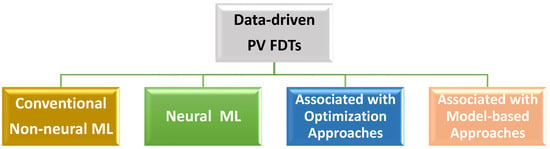
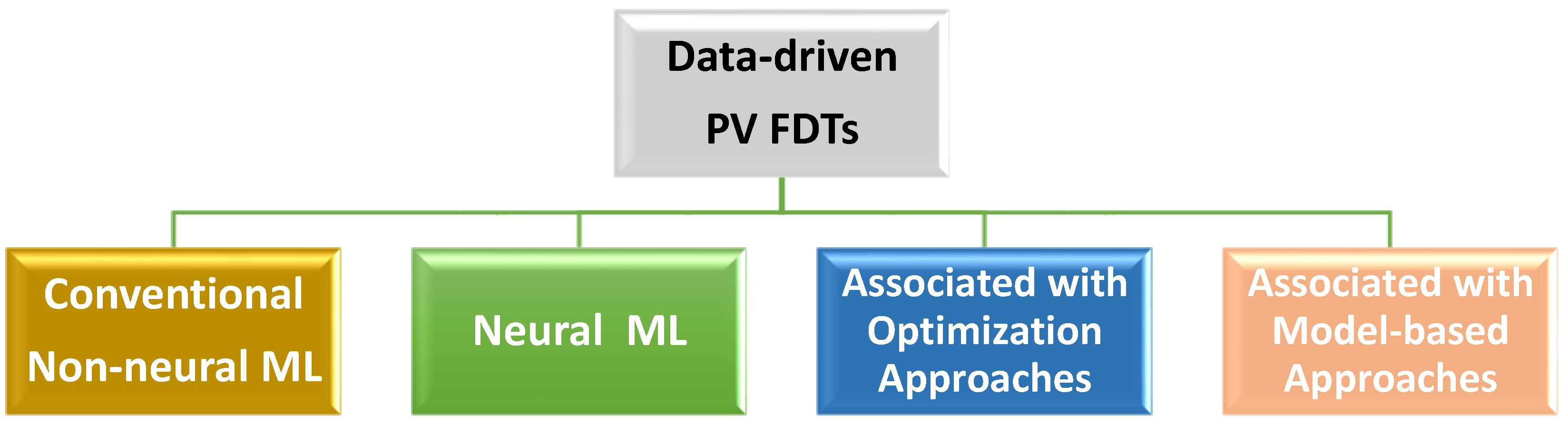
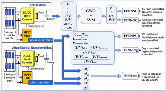
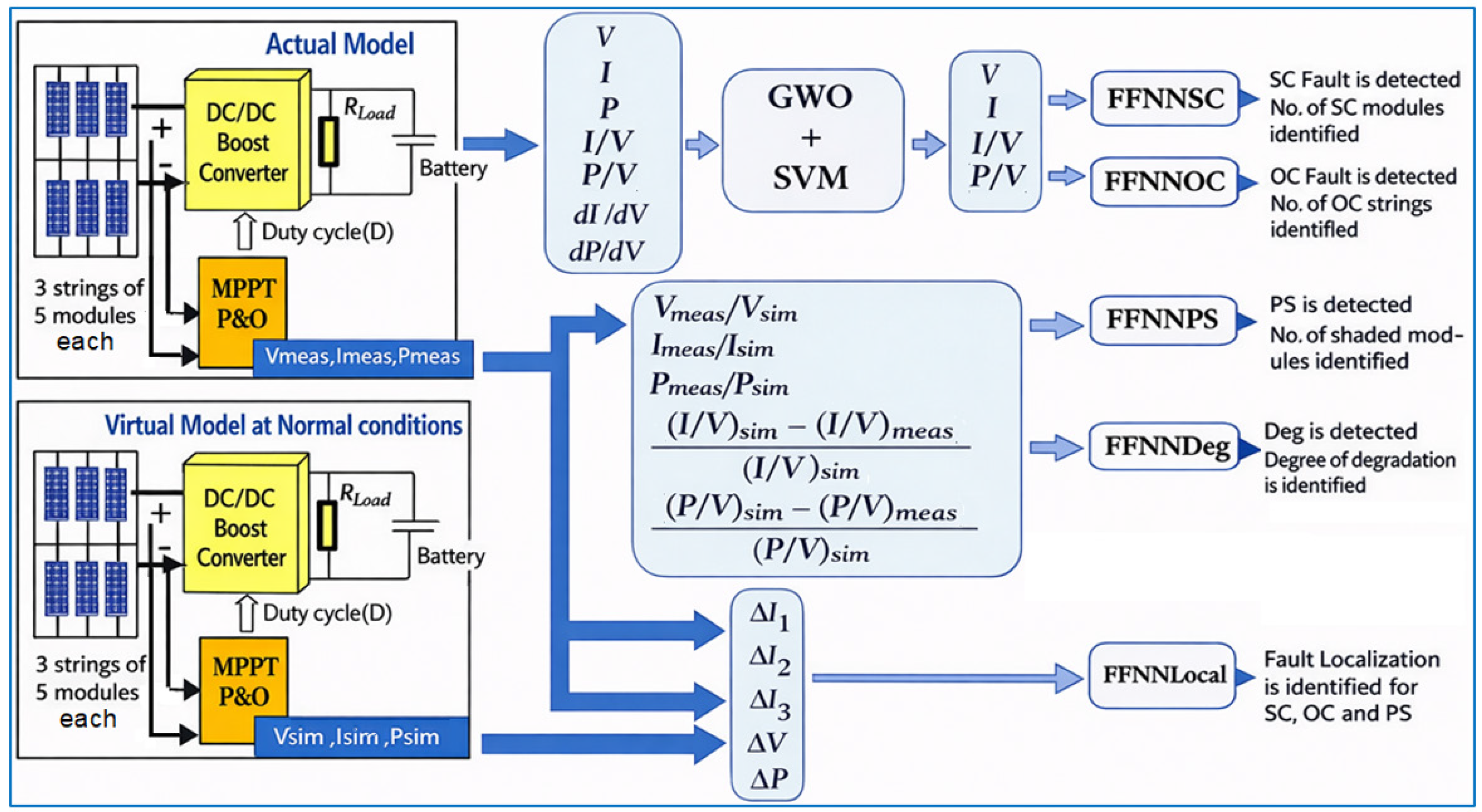
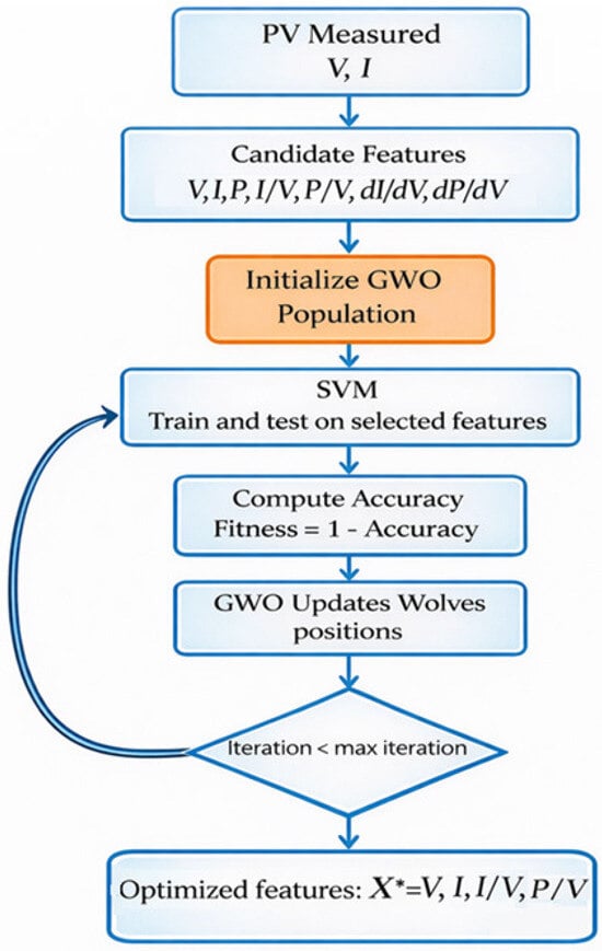
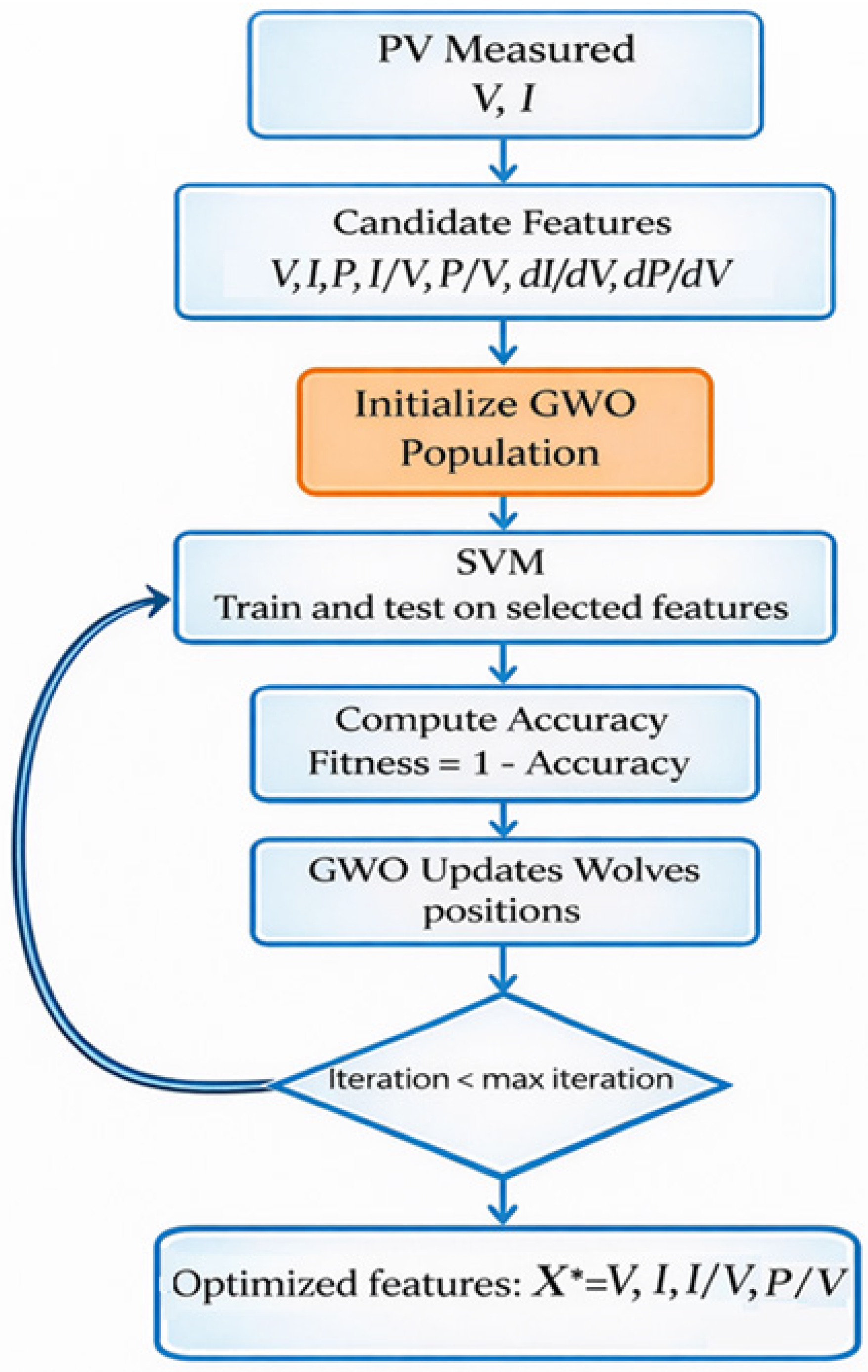
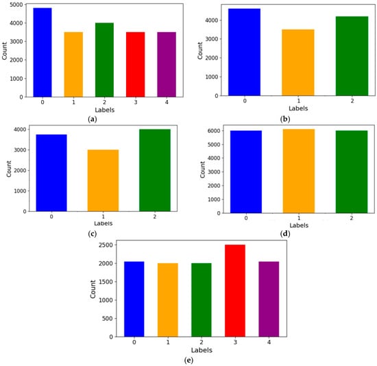
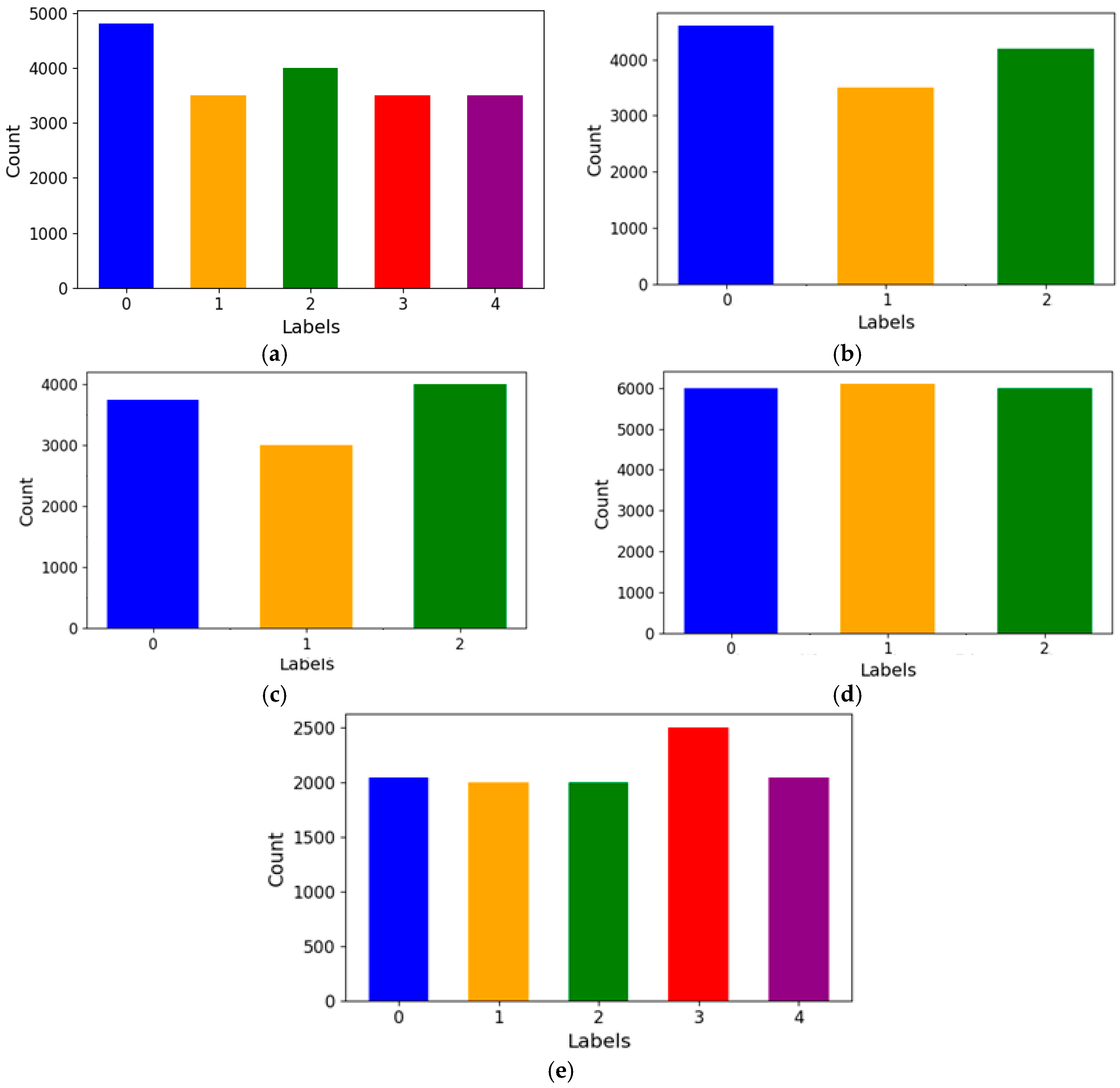
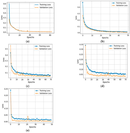
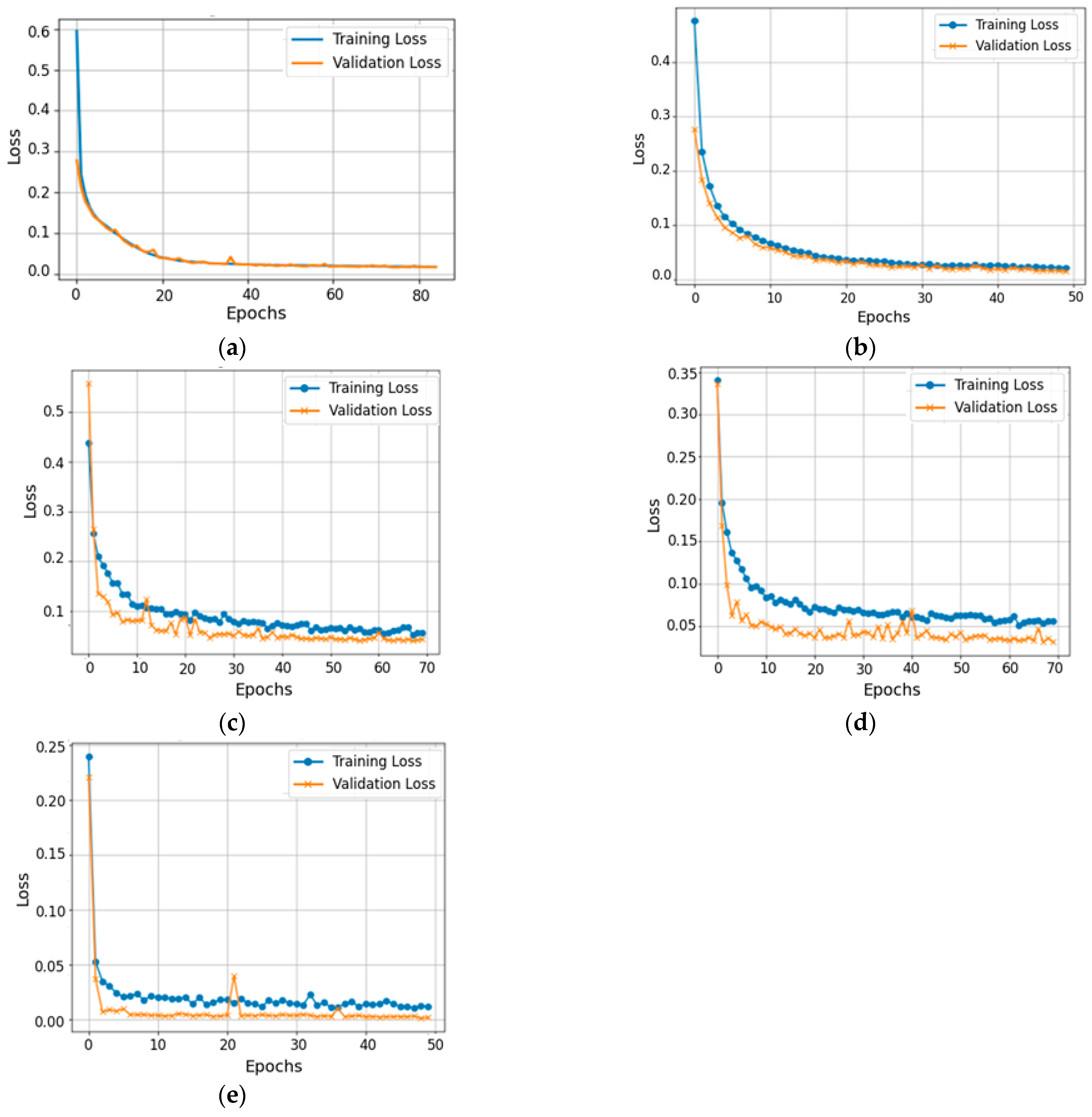
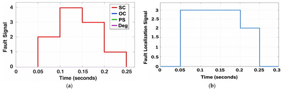
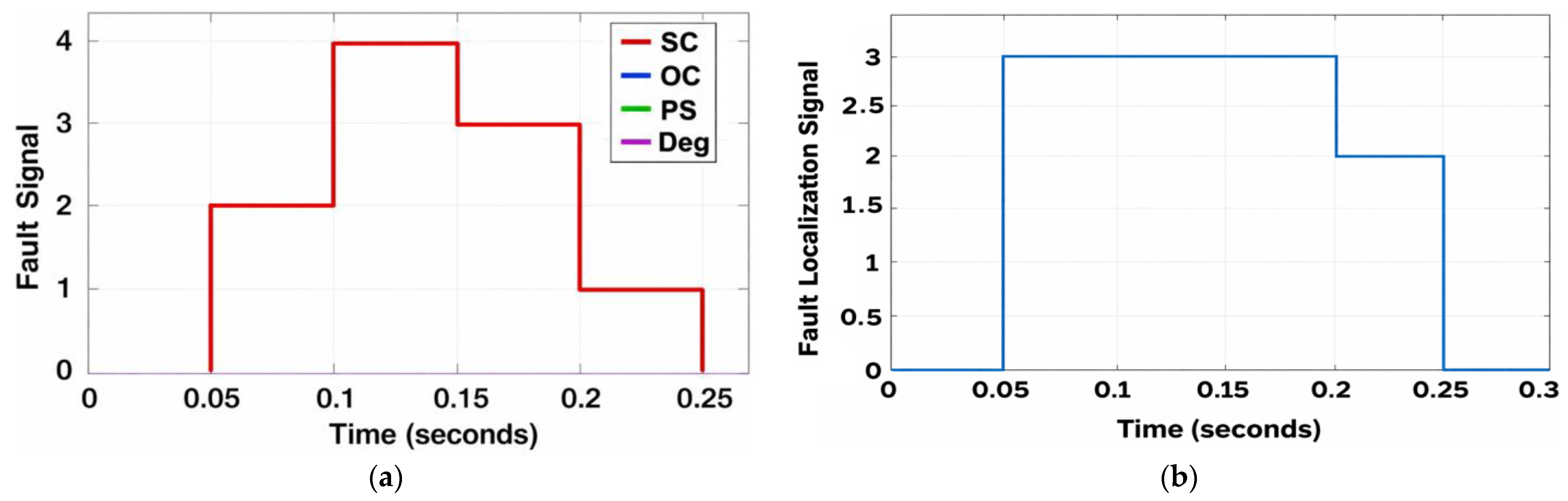
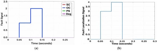
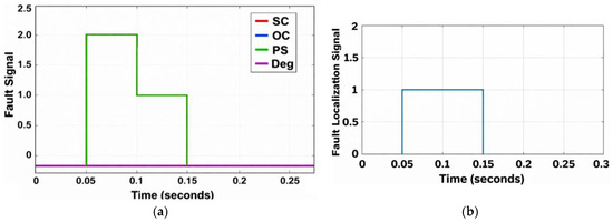
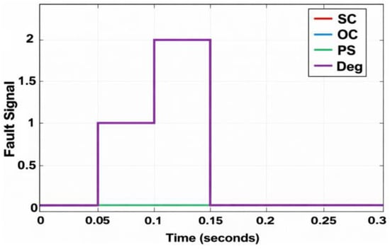
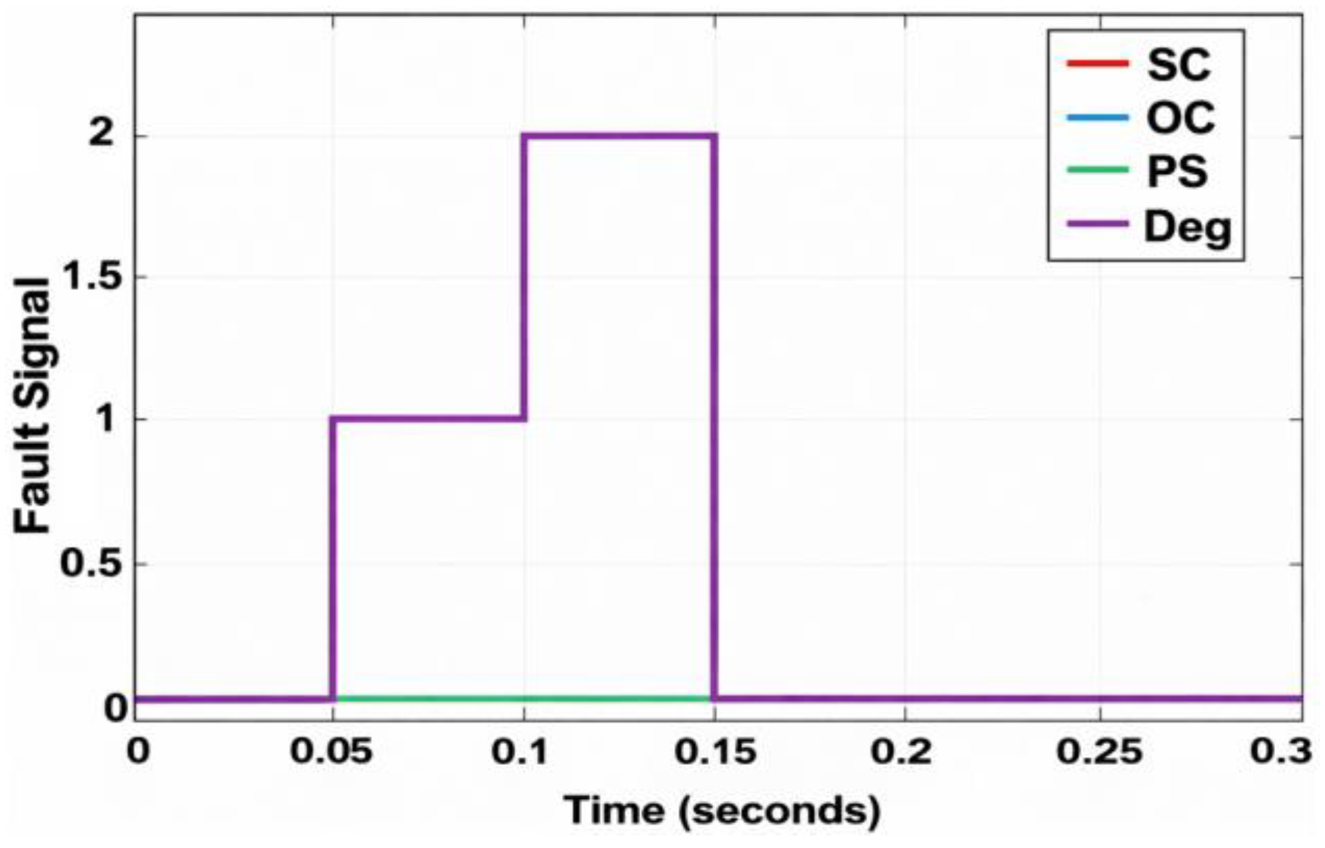
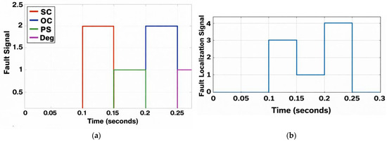
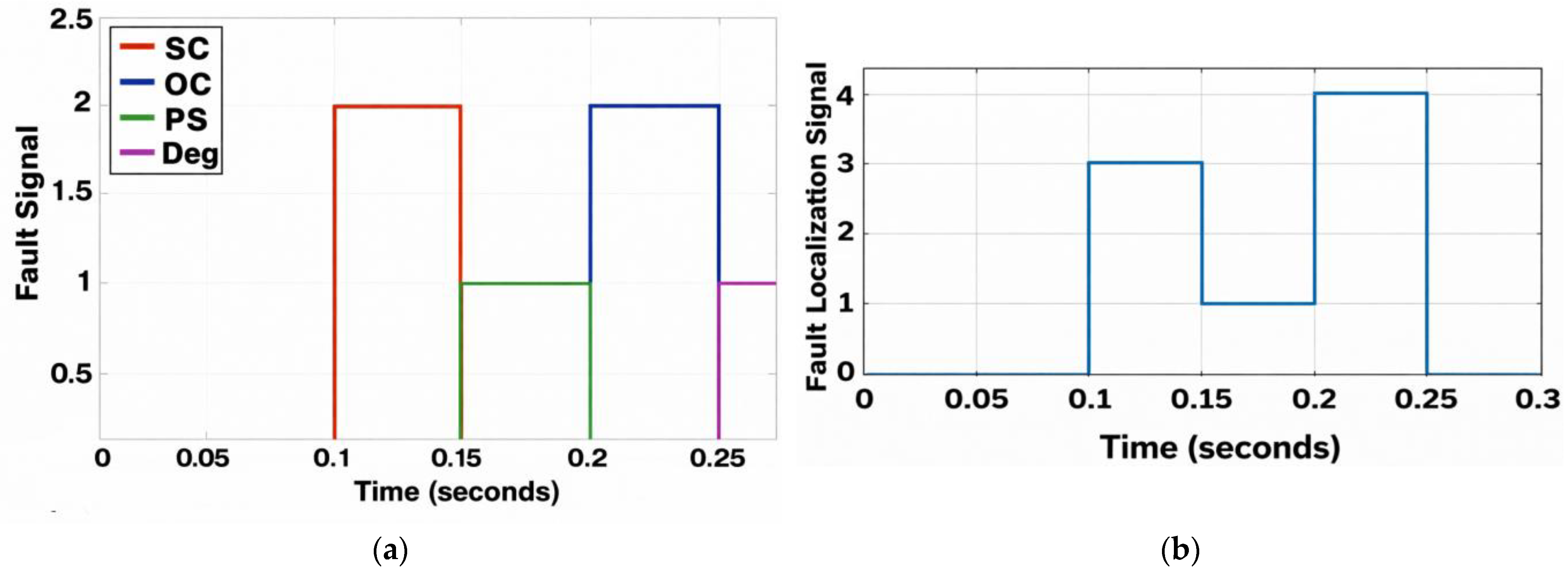
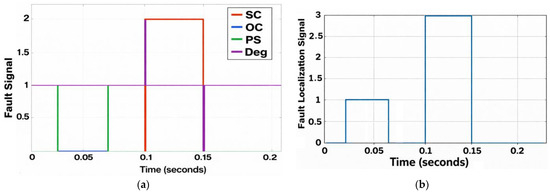
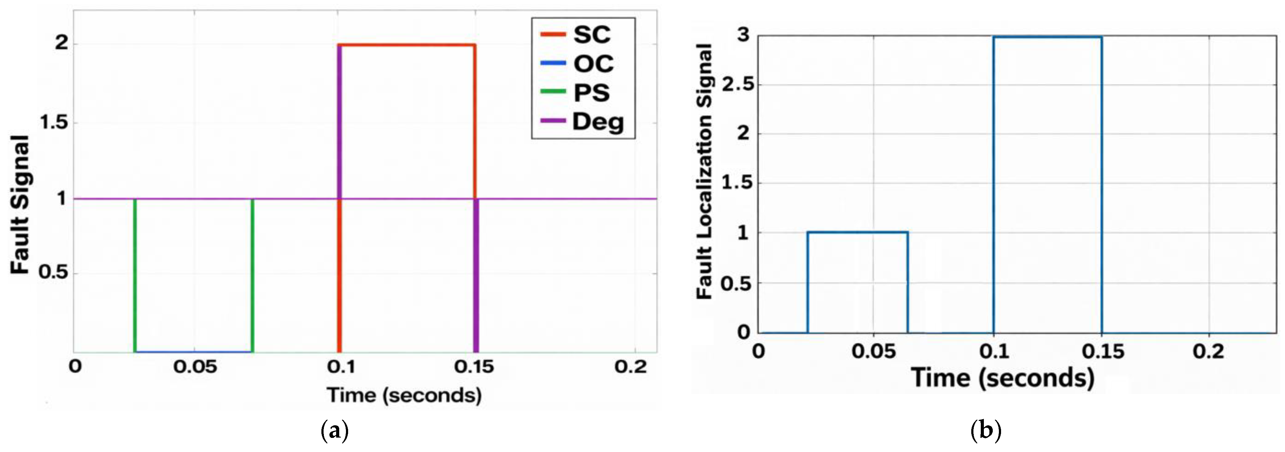
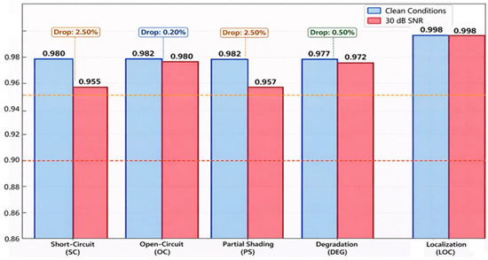
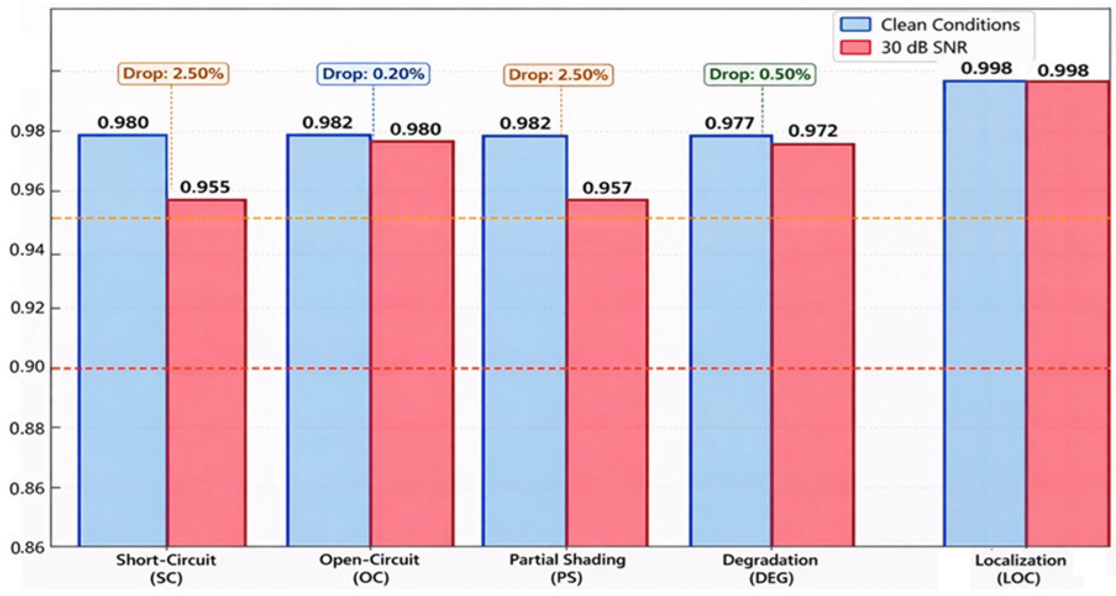
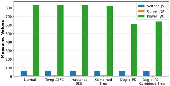
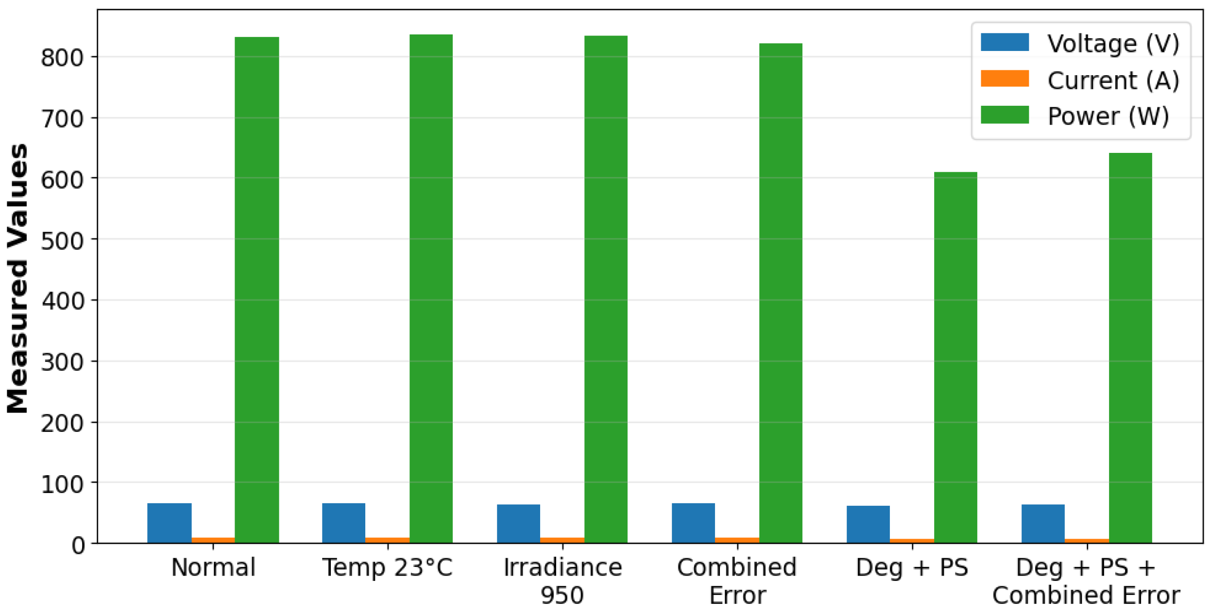

Disclaimer/Publisher’s Note: The statements, opinions and data contained in all publications are solely those of the individual author(s) and contributor(s) and not of MDPI and/or the editor(s). MDPI and/or the editor(s) disclaim responsibility for any injury to people or property resulting from any ideas, methods, instructions or products referred to in the content. |
© 2026 by the authors. Licensee MDPI, Basel, Switzerland. This article is an open access article distributed under the terms and conditions of the Creative Commons Attribution (CC BY) license.