


Abstract
Campaign-level assessments of human lunar exploration architectures are commonly performed over finite horizons, which can conceal systematic buffer drawdown and asset drift beyond the simulated window. This paper presents a reproducible methodology in which sustainability is formalized as a periodic (steady-state) property of the coupled inventory–asset system, defined with respect to the modeled state variables and enforced as a binary feasibility gate on all performance evaluation. The architecture is represented as an event-driven multi-commodity flow over a reduced, SpaceNet-compatible network, equivalent to a time-expanded formulation, with propellant demand coupled to transported mass through the rocket equation. Standard measures of effectiveness are augmented with three dimensionless indicators and a composite index whose alignment with the dominant principal component of the trade space is tested a posteriori. On an Artemis III-derived case study the reference cycle closes (, 32.3-day margin), yet 18 of 81 nominally feasible design points lose periodic sustainability under launch-delay perturbations, all 18 classifications being statistically significant at the 95% level. Periodic-state closure thus provides a formal criterion for cycle-to-cycle depletion that requires no arbitrary horizon choice. Applied unchanged to three architectures spanning nearly seven-fold in launch mass, the analysis shows an expendable direct-descent concept leading every mass-normalized indicator at a fixed two-crew objective, an ordering that is stable under dry-mass and specific-impulse perturbations, while a Gateway hub becomes preferable once orbital infrastructure and extensibility are valued. This study regenerates deterministically from a single input dataset.
1. Introduction
1.1. Motivation: From Mission Feasibility to Campaign Sustainability
The return of human crews to the lunar surface under NASA’s Artemis program requires an integrated logistics architecture. The publicly described Artemis III concept of operations relies on an intensive pre-deployment chain—an Earth-orbit propellant depot, a series of reusable tanker flights, and the transit of the Starship Human Landing System (HLS) to a Near-Rectilinear Halo Orbit (NRHO) before crew arrival—followed by rendezvous, surface expedition, and Earth return [1,2]. Each additional launch, proximity operation, and propellant transfer increases total launch mass and risk exposure, which motivates evaluation with explicit logistics performance and risk measures [3,4].
Most campaign studies, however, assess feasibility over a finite horizon: a scenario is declared feasible if demands are met and vehicles close their propulsive budgets within the simulated window [4,5]. A campaign may satisfy every constraint inside the window while systematically drawing down consumable buffers, stranding assets in non-recoverable configurations, or accumulating propellant deficits that become binding one or two cycles later. For a program whose stated ambition is sustained presence [2,6], feasibility must be redefined. The relevant question is not whether one mission closes, but whether the campaign admits a periodic operating regime in which inventories, asset positions, and crew presence repeat cycle after cycle without depletion. The problem addressed in this paper is how to decide whether a lunar campaign architecture admits such a repeatable operating regime, and how to compare structurally different architectures on that basis in a reproducible way.
Throughout, periodic sustainability denotes the closure of the modeled logistics state over one campaign cycle: inventories, tracked asset positions, and crew presence return to their initial configuration. It is a property of the logistics loop and does not imply material circularity. The life-support model is an open-loop consumables proxy, all commodities are imported from Earth, and no recycling or in situ resource utilization is modeled, so the concept is distinct from the closed material loops of a circular space economy. Section 2.3.3 states the modeled state variables, and all sustainability claims are made with respect to them.
1.2. Related Work
Network-based space logistics modeling originates in the interplanetary supply chain framework of Gralla, Shull, and de Weck [7] and in its consolidation in the SpaceNet simulation environment [4,8,9], which has more recently been extended to a web-based deployment for large-scale exploration analysis [10]. SpaceNet represents exploration as a discrete-event flow of elements and supply classes over nodes and arcs and introduced the measures-of-effectiveness (MOE) suite adopted here [3]. On the optimization side, Taylor et al. formulated interplanetary mission planning as a mathematical program over a logistics network [11]. Ho et al. introduced time-expanded network formulations for campaign-level optimization [12,13], and Ishimatsu et al. generalized the framework to multi-commodity flows with commodity transformation (the generalized multi-commodity network flow, GMCNF, model) for the Earth–Moon–Mars system [14]. Subsequent work coupled logistics network optimization with vehicle design [15], with in-situ resource utilization (ISRU) system sizing [16], with multifidelity planning and infrastructure design [17], and with mixed high-/low-thrust propulsion through event-driven network models [18], while operations under demand and schedule uncertainty have been addressed through servicing-optimization frameworks [19]. The review by Ho [20] consolidates this field and notes that validating its simplified trajectory, vehicle, and operational models against higher-fidelity simulations remains a largely unexplored need, one which reproducible and openly executable tools directly address. Graph-theoretic representations of space architectures are surveyed in [21]; the selection of NRHO as the Artemis staging orbit is established in [22,23,24,25], high-fidelity Gateway-to-low-lunar-orbit transfers in [26], and reliability- and supportability-driven logistics in [27,28].
Two gaps persist in this literature. First, periodic boundary conditions are absent. With the partial exception of steady-state resupply analyses for the International Space Station [29], campaign formulations impose initial conditions and terminal requirements but do not require the terminal state to reproduce the initial state, so finite-horizon feasibility can mask structural unsustainability. Second, evaluation and exploration are decoupled from reproducibility. Published campaign studies are rarely regenerable from their inputs, and scenario assumptions such as orbit proxies, arc-cost proxies, and element parameterizations are seldom enumerated with the completeness required for independent verification, a deficiency the reproducibility literature has documented across computational science [30].
1.3. Contributions
This paper addresses both gaps with three scientific contributions and one implementation contribution.
- 1.
- Periodic sustainability as a first-class feasibility criterion (Section 2.3). Sustainability of a campaign cycle is formalized as cyclic boundary conditions on commodity inventories and tracked asset positions, combined with continuous surface presence, non-depletion, and surface-objective constraints, and condensed into a binary feasibility gate z that conditions all performance evaluation. The results show empirically that this gate, combined with schedule perturbation, exposes architectures that are nominally feasible yet operationally unsustainable (Section 6.4).
- 2.
- An augmented indicator suite with an a-posteriori consistency test (Section 3). The classical MOE suite [3] is extended with three dimensionless indicators—propellant-specific science return , supply resilience , and Monte Carlo schedule-delay robustness R—and a composite Sustainable Exploration Return Index (SERI) whose alignment with the dominant principal component of the evaluation space is tested a posteriori rather than asserted.
- 3.
- A reproducible scenario-exploration pipeline (Section 4 and Section 6). A full-factorial design of experiments is simulated, evaluated, and analyzed with principal component analysis (PCA) [31], Gaussian mixture archetype identification with information-criterion model selection [32], Pareto non-dominance in the sense of [33], and main-effect screening, end to end and deterministically from a single comma-separated values (CSV) input dataset.
In addition, the SpaceNet database schema [9] is reduced to the fields required for campaign-level analysis and implemented in an openly released program (Section 2.2), which enables programmatic scenario sweeps that the original graphical environment does not support at scale. This is an engineering enabler rather than a scientific result. Table 1 separates what the work inherits from the SpaceNet framework from what it introduces.
Table 1.
Provenance of the methodological components.
The Artemis III-derived periodic architecture is the primary demonstration case. The methodology itself is architecture-agnostic, and Section 6.7 demonstrates this by comparing three structurally different concepts—the reusable two-lander baseline, an expendable direct-descent architecture, and an NRHO/Gateway hub—under one common indicator suite and feasibility gate, each instantiated in its own CSV input dataset with no change to the engine.
2. Methodology: Representation and Mathematical Formulation
2.1. Network Representation
The physical system is represented as a static directed graph , where nodes are surface or orbital locations and directed arcs are abstracted transport opportunities characterized by a duration and a set of impulsive burns with velocity increments . This representation follows the SpaceNet convention [8,9]: arcs encode logistics-relevant transfer costs, not physical trajectories, which is the appropriate abstraction level when the object of study is campaign structure rather than astrodynamics [21]. Following the SpaceNet data model, self-loops and duplicate arcs per origin–destination pair are not represented. Loiter, docking, and surface-stay phases are node-level dwell processes (assumption E-1, Section 2.4). Dynamics are introduced through the implicit time expansion of the event engine: an element traversing arc a departing at t occupies the arc during , which is the discrete-event equivalent of the time-expanded network formulations of [12,14]. The advantage of the implicit expansion over an explicit time-expanded graph is computational: scenario sweeps require thousands of cycle simulations, and the event-driven engine evaluates a cycle in milliseconds because the continuous dynamics between events are piecewise linear and integrated in closed form (Section 4.1). The formulation evaluates a given event schedule and does not optimize routing decisions. Exact mixed-integer linear programming (MILP) optimization of the manifest over the expanded network [11,15] is deferred to future work (Section 7).
2.2. Reduced SpaceNet-Compatible Data Model
The full SpaceNet database schema [9] comprises nine object classes with over sixty fields, most of which are not needed at campaign level. The retained field set preserves semantic compatibility in both directions. Nodes carry an identifier, type, name, body, and either a georeference or the Keplerian descriptors (apoapsis, periapsis, inclination); edges carry origin, destination, duration, and distance; burns carry their edge, ordering time, and ; and elements carry type, Class of Supply, environment, masses and volumes, crew and cargo capacities, active fraction, specific impulse, and tank capacity, extended with the explicit initial-state fields (initial_fuel, initial_node, initial commodity loads, and the tracked flag) that the periodic formulation requires.
Commodities are mapped to SpaceNet Classes of Supply (COS): propellants (COS 1), aggregated crew consumables (COS 2/3), science payload and returned samples (COS 6), stowage (COS 5), habitation infrastructure (COS 8), and transportation elements (COS 9) [34]. The entire scenario—network, elements, mission timeline, and simulation parameters—is contained in a single CSV input dataset (one plain-text table per entity), which is the only artifact a user edits (Section 4). The structure of these tables and the meaning of their fields follow the SpaceNet database schema as documented in the SpaceNet User’s Guide [9], to which the reader is referred. The two departures from that schema, the explicit initial-state fields listed above and the mission-timeline event grammar executed by the engine of Section 4.1, are documented in the input guide distributed with the released datasets.
2.3. Mathematical Formulation
2.3.1. State, Flows, and Commodity Balance
Let denote the tracked commodity set, the element set, and one campaign cycle. The system state is
where is the location of element p (a node, an arc, or a disposed/recovered terminal state), its onboard propellant, the inventory of commodity k at node i, and the surface crew count. Between events, inventories obey the piecewise-linear balance
where [kg crew−1 day−1] is the consumables rate (an open-loop environmental control and life support system, ECLSS, proxy of the order of the NASA space logistics consumables model referenced in [9]), [kg crew−1 day−1] the sample-acquisition rate, and the mean crew active fraction (0.66, assumption EL-2 in Section 2.4). Campaign-level sustainability is governed by integrated consumption and delivery rather than by sub-daily ECLSS dynamics, and any higher-fidelity demand model [9] can replace the right-hand sides without altering the formulation. Discrete events (transports, transfers, refuelings) introduce jump discontinuities in at their scheduled epochs.
The scope of the state vector in Equation (1) bounds every sustainability claim in this paper. The tracked quantities are element positions, element propellant, node inventories of the modeled commodities, and the surface crew count. Waste streams, hardware degradation, maintenance demand, spares, and accumulated component failures are not state variables, and transit consumables are provisioned within vehicles and untracked (assumption H1). A campaign that closes in the tracked variables could therefore still degrade in an unmodeled one, and the periodicity conditions of Section 2.3.3 certify sustainability with respect to the modeled state variables and constraints, not absolute campaign sustainability. Extending the state vector with consumable-hardware and sparing states [28] is the natural refinement (Section 7.3).
2.3.2. Propulsive Coupling
Each burn b executed by a designated burner element with specific impulse on a stack of instantaneous wet mass consumes propellant according to the ideal rocket equation [36]:
where sums the dry masses, residual propellants, crew, and carried commodities of every element in the stack. Equation (3) couples the commodity flows to the transport decisions and produces the characteristic logistics nonlinearity, in which propellant carried for later burns inflates the cost of earlier ones, that motivates staged refueling in the Artemis concept [1]. Burns are impulsive and arc costs are fixed proxies (assumption H4, Section 2.4). The fidelity trade is discussed in Section 7.3.
2.3.3. Periodic Sustainability and the Feasibility Gate
The central definition of this paper is the following. A cycle of length is sustainable if and only if the trajectory of (1) satisfies simultaneously:
The feasibility gate is
Three modeling choices in (4) and (5) require justification. First, periodicity is imposed on tracked subsets : expendable elements replenished one-for-one each cycle are excluded from (5) and their cost is charged entirely to Total Launch Mass (H2), the accounting-consistent treatment of a replenished fleet. Second, (5) is stated on the position multiset (): in the demonstration architecture two identical landers exchange roles each cycle, so element-wise periodicity holds only over two cycles while the multiset {surface, staging orbit} is invariant every cycle (H5). Third, the returned-sample stock is permitted to grow, so samples are excluded from while remaining subject to (8) (H3). Tolerances—one crew-day-equivalent of consumables for (4) and a declared propellant band for lander fuel states—absorb the sub-percent numerical residue of the piecewise integration and are reported with the input file.
The gate z is deliberately binary rather than graded. Sustainability, like structural integrity, is an admissibility property. A campaign that violates (7) for one day is not “mostly sustainable”: it fails, and blending the violation into a continuous score would reintroduce the compensability the formulation is designed to exclude. Graded information about how close a feasible campaign is to failure is instead carried by the margin and resilience indicators of Section 3.2.
2.3.4. Margin Metric
2.4. Consolidated Assumptions and Parameter Provenance
Table 2 consolidates the assumptions and parameters of the study and classifies each entry as a modeling hypothesis, a scenario assumption, a model parameter, a derived value, or an externally sourced value. The numbering is contiguous, every in-text code refers to this table, and the same register is embedded in the released input datasets. Element masses, propellant loads, and event epochs are given in full in the input files, in Table 3 and Table 4, and, for the alternative architectures, in Section 6.7.
Table 2.
Consolidated assumption and parameter register. Categories: H = modeling hypothesis; A = scenario assumption; P = model parameter; D = derived value; S = externally sourced value.
Table 3.
Scenario nodes (reduced SpaceNet schema). Orbital apoapsis/periapsis are altitude descriptors in km; echoed verbatim from the input file.
Table 4.
Directed transport arcs and impulsive burn proxies. values follow standard cislunar reference profiles [9] and the NASA NRHO profile [25]. Durations are in days, and the assumption codes refer to Table 2.
3. Evaluation Framework
3.1. Classical Measures of Effectiveness
The classical suite follows the MIT Space Logistics Project definitions [3], retained verbatim to anchor the augmented framework to community-accepted metrics. Crew surface days (CSD), total launch mass (TLM), exploration mass delivered (EMD), upmass capacity utilization (UCU), exploration capability (EC), relative exploration capability (REC), relative scenario cost (RSC) and element active days (EAD) are defined, over one cycle, as follows.
where CSD is in crew-days, EMD and TLM in kg, EC in kg crew-day, UCU in , is the summed element-active-days and the cost weights, both unity here. With unit weights the launch-mass term dominates RSC (the fleet term contributes under of the numerator, so ); RSC is therefore reported but not treated as an independent axis, a near-duplication accounted for in Section 6.5. In Equation (15), are the counted launches, docking/refueling operations, and landings, and the per-event success probabilities (, , ; with the baseline counts of Table 5 these give ). Event independence is a declared simplification standard in campaign-level risk aggregation [3,28]. The Apollo 17 normalization constants of Table 2 are taken from the mission record [35] and exposed as parameters, since REC and RSC are only meaningful relative to a documented baseline.
Table 5.
Baseline evaluation vector of the Artemis III–derived periodic cycle. Risk is computed at the modeled event counts under H2 (see Section 6.7 for the resolved physical counts).
3.2. New Indicators
Three indicators, absent from the classical suite, capture dimensions that the periodic formulation makes measurable. All are dimensionless (or day-normalized) and defined only for .
3.2.1. Propellant-Specific Science Return
With the sample mass returned to Earth per cycle and the cycle propellant expenditure,
measures the sample return obtained per kilogram of propellant expended. Because is dominated by the Earth-to-orbit ascent burns (about of the 9987 t baseline total), correlates strongly with total launch mass and discriminates between architectures mainly through their imported propellant budget rather than through refueling alone, as Section 6.5 and Section 6.7 confirm.
3.2.2. Supply Resilience
With m the margin of (12),
the minimum consumables margin normalized by cycle length. quantifies how close to depletion the architecture operates in nominal conditions and is the deterministic precursor of robustness.
3.2.3. Schedule-Delay Robustness
Launch delays displace the entire operational chain (launch, aggregation, transit, handover, resupply), extending the outgoing crew’s surface stay against a fixed pre-resupply stock. With delays drawn as , a half-normal schedule-perturbation proxy, the schedule-delay robustness is the Monte Carlo estimate
The perturbation model covers launch delays only, and since propellant budgets are delay-invariant under fixed arc proxies (H4), the sole failure channel is depletion of the logistical stock. R is therefore a schedule-delay and reserve robustness metric, not a measure of overall architectural robustness: vehicle-loss contingencies, reliability dynamics, and demand uncertainty lie outside its uncertainty model (Section 7.3). Within that scope, R separates designs indistinguishable in the nominal case. Every reported R is a binomial estimate accompanied by its 95% Wilson interval, with sample sizes declared in Table 2.
3.3. The Sustainable Exploration Return Index
The composite indicator is the base-normalized product
so that and for any unsustainable architecture. The multiplicative form is non-compensable (any factor approaching zero collapses the index) and needs no free weights, but any aggregation imposes a preference structure, so SERI is not the comparative foundation of this work. Rankings are based on the Pareto front over the objective vector
and SERI is subjected to an a posteriori consistency test: its correlation with the first principal component of the standardized evaluation matrix is reported with a bootstrap confidence interval (Section 6.6). Two caveats limit what this test can establish. The first principal component (PC1) is the direction of maximum variance of the same evaluation matrix, not an external reference, and SERI is built from metrics that belong to that matrix, so the test is partly circular. It can refute a grossly misaligned index but cannot validate SERI in the model-validation sense of Section 4.3. The correlation is therefore reported as a descriptive alignment statistic rather than judged against a pass/fail threshold, the stability of the SERI ranking under alternative constructions is examined, and a weak alignment would lead us to report only the Pareto front.
3.4. Cross-Architecture Comparison Methodology
Structurally different architectures are compared under four devices, applied in order: (i) the common feasibility gate z; (ii) baseline-relative normalization, which renders topologically different networks commensurable; (iii) projection into a common principal-component space; and (iv) Pareto dominance over (20). Device (iii) also tests the indicator suite itself: if the classical MOEs are collinear while the new indicators load on distinct components, the new indicators add information the classical suite does not carry. Section 6.5 finds this to hold for , the margin, and R, but only partially for .
4. Simulation Platform and Reproducibility Protocol
4.1. Architecture
The reference implementation is a sequential, open-source program operating on the single CSV input dataset, with modules that map one-to-one onto the methodology: input loading and validation, model construction, the discrete-event engine implementing Equations (1)–(10) (elements in transit are credited to the destination node only from the arc’s arrival time, so surface crew days accrue from landing), one evaluation function per metric, the Monte Carlo layer of (18), the full-factorial scenario generator with its internal-consistency rules, a multivariate layer (standardization, singular value decomposition, SVD, based PCA [31], expectation–maximization, EM, Gaussian mixtures with information-criterion selection [32], Pareto filtering [33]), and an export layer that writes every figure, table, a JavaScript Object Notation (JSON) metrics record with the input manifest, a log, and a report. Only mature open scientific libraries are used, and the multivariate algebra is implemented in numpy so that no machine-learning framework is required.
4.2. Input Validation Layer
Before any simulation, the platform validates mandatory-field completeness, units and physical ranges, network referential integrity, the propulsive capability of every burner, the temporal ordering of the timeline, a positional pre-simulation that verifies each event finds its elements at the required node (the discrete-event analogue of SpaceNet’s pre-simulation [9]), and the expected periodic consumables balance. Every failure reports the table, row, field, and corrective action.
4.3. Verification and Validation Status
The evidential status of the platform is stated in the standard three-level vocabulary. Software verification: the input-validation layer of Section 4.2 checks field completeness, physical ranges, referential integrity, propulsive capability, temporal ordering, and the positional pre-simulation, and every propellant budget is re-verified against Equation (3) at each execution. Internal consistency verification: the periodic-state computation of Section 6.2 (fixed point, contraction, multi-cycle propagation with sub-kilogram residuals) establishes that formulation and implementation are mutually consistent, and the Artemis III-derived case is treated throughout as a demonstration of this consistency. Model validation against an independent implementation, a higher-fidelity trajectory tool, a reference campaign, or flight data has not been performed and is not claimed; the review by Ho [20] identifies this as a largely unresolved need for the field. The sourced values of Table 2 tie the scenario to published data but do not validate the model outputs; the contribution of the released platform is a regenerable baseline against which such validation can be performed.
4.4. Reproducibility Protocol
Reproducibility is enforced by construction rather than by policy [30]: the CSV input dataset is the sole input and is version-controlled with the code, all stochastic layers are seeded from a single declared seed, every figure and table of this paper is a file in the Results/ tree regenerated by a single execution, the assumption register of Table 2 is embedded in the input file, and the execution log records a SHA-256 digest of every input table actually read, so the provenance of a results tree can be checked against the distributed inputs file by file.
5. Demonstration Case: An Artemis III-Derived Periodic Architecture
5.1. From Artemis III to a Periodic Operating Regime
Artemis III, as publicly described, is a single sortie: four crew travel to lunar orbit, two descend, and all four return [1]. A sustained campaign requires an operating regime that repeats. The demonstration case therefore evolves the Artemis III element set into a periodic architecture defined by three features. First, continuous surface presence with paired rotations: each cycle launches a crew pair, overlaps it on the surface with the outgoing pair during handover (: ), and returns the outgoing pair with the accumulated samples; the four-crew Artemis III sortie is the documented bootstrap mission preceding the periodic regime and is not itself simulated. Second, a two-lander HLS fleet alternating between the surface and the staging orbit: the orbiting, refueled lander descends with the incoming pair while the surface lander ascends with the outgoing pair, is refueled, and becomes the next cycle’s descent asset, so that each lander executes one powered leg per cycle, which renders the propellant budget closable (a single lander executing all legs was found to be propulsively infeasible under the declared proxies). Third, aggregated cislunar propellant delivery: a cargo/tanker element, the accounting-level aggregation of the NASA depot-plus-tankers concept [1], delivers the lander refueling load, crew-vehicle top-off, and logistics upmass, and is expended (H2).
5.2. Network Instantiation
The scenario network consists of six nodes and six directed transport arcs, defined in Table 3 and Table 4 and shown in Figure 1; the assumption codes refer to Table 2.
Figure 1.
Earth–Moon logistics network of the periodic scenario (schematic layout). Generated by the program from the node, edge, and burn definitions in the input file. Node codes (KSC, Kennedy Space Center; LEO, low-Earth orbit; LLPO, low-lunar polar orbit; LSP, lunar south pole; PAC, Pacific splashdown node) are as in Table 3.
Each row of Table 3 gives the node identifier and name, the celestial body, and, for orbital nodes, the apoapsis and periapsis altitudes and the inclination as read from the input file; surface nodes carry a georeference instead. The launch origin uses the KSC LC-39A coordinates (N-1), the low-Earth-orbit staging and aggregation nodes use the km, i = 28.5° orbit of the SLS DSNE specification (N-2), the recovery node is a Pacific splashdown proxy (N-6), and the surface node is a Shackleton-region south-pole proxy (N-5). The lunar staging node is encoded as a 100 km circular polar low lunar orbit (LLPO), a Keplerian descriptor compatible with the reduced schema, while the and time of flight of the arc that reaches it absorb the reference NRHO insertion profile, so that the node is cost-equivalent to the Artemis NRHO staging orbit (N-3/N-4); this mapping is a declared modeling proxy.
Table 4 lists the arcs with their transit time, a geometric distance proxy (E-2), and the total impulsive , decomposed in the last column into burns. The KSC–LEO arc carries an aggregated 9500 m/s surface-to-LEO cost (B-1). The translunar arc combines the 3150 m/s trans-lunar injection with the 450 m/s staging insertion, modeled as two 225 m/s burns following the reference NRHO profile (B-2). Mid-course corrections are absorbed into the arc proxies (B-3), the powered-descent and ascent arcs carry the 2030 and 1875 m/s reference costs, and the return arc aggregates trans-Earth injection and entry. All values are fixed proxies under H4 and the absolute propellant figures inherit their uncertainty (Section 7.3).
5.3. Element Set and Closable Propellant Budgets
The thirteen scenario elements (crew vehicle with 316 s hypergolic-class service propulsion; a 462 s cryogenic upper stage performing TLI, Interim Cryogenic Propulsion Stage (ICPS) class; aggregated crew and cargo launch stacks at 430 s; two 100-t HLS landers at 380 s; the expendable tanker; a pressurized logistics carrier; a pre-deployed surface habitat holding the consumables reserve and sample backlog; and four tracked crew members at the 100 kg SpaceNet convention) are listed with their full parameterization in the input file. Initial propellant loads were sized ex ante by backward propagation of Equation (3) along each element’s burn sequence and are re-verified by the engine at every execution (Equation (9)). Two sizing results carry architectural meaning: the per-cycle lander refueling load at the staging node is 188 t, so the aggregated tanker requires about 680 t of propellant in LEO, which is why the cargo launch stack (H2) dominates cycle launch mass (Section 6.1).
5.4. Mission Timeline
The 20-event cycle timeline is fully specified in the mission_timeline table of the input file, with its parameter references resolved against the parameter table, and is the sequence read chronologically from Figure 2. The steady-state design values are exposed as editable parameters: a consumption rate of 7 kg crew−1 d−1 [9], a 45-day reserve, a 1274 kg resupply per cycle equal to the expected 182 crew-day cycle demand, 100 kg of science upmass, and a 144 kg sample export equal to the expected cycle generation.
Figure 2.
Element time-location chart of the reference cycle, showing all thirteen scenario elements. Small vertical offsets separate traces that share a location, the left panel expands the event-dense active phase (days −1 to 18), and the right panel compresses the static remainder of the 90-day cycle. Dashed traces are crew. The vertical axis carries physical locations only: disposal (REMOVE) and recovery (RECOVER) are marked by cross and down-triangle glyphs at the location where they occur, where the corresponding trace ends. The HLS_A/HLS_B traces exchanging the LSP and LLPO levels visualize the position-multiset periodicity of Equation (5).
6. Results
All quantitative results in this section are outputs of the reference execution of the released program on the reference input file; they are not asserted values, and re-executing the program regenerates every number, figure, and table reported below.
6.1. Baseline Cycle: Sustainability Closure
The baseline cycle satisfies the full feasibility gate () with zero propellant violations, continuous presence throughout, no depletion, and the sample objective met. All periodic conditions are satisfied to numerical precision rather than merely within tolerance. The periodic state is computed rather than assumed (Section 6.2). The terminal consumables stock returns to its initial 630 kg level with a residual below kg against a 14 kg tolerance, the tracked lander propellant states return to their initial values t with a residual below kg against a 5 t tolerance, the lander position multiset {LSP, LLPO} is invariant, and two crew are on the surface at . The minimum consumables margin is days (). Cycle totals are m/s executed, t, and t across two modeled launches, six docking or refueling operations, and two landings. Table 5 reports the complete evaluation vector. Risk in Table 5 is computed at the modeled event counts under the launch-aggregation hypothesis H2. When the aggregated cargo launch is resolved into its physical flights, as in the cross-architecture comparison of Section 6.7, the baseline value rises from 0.087 to 0.191.
6.2. The Periodic State: Fixed Point and Multi-Cycle Propagation
A declared tolerance on the periodicity conditions invites an objection: a residual small enough to pass the gate but systematically signed would accumulate over successive cycles. Two results address it. First, the periodic state is computed rather than assumed. Writing the cycle as a return map that carries the propellant loads of the tracked fleet from the start of a cycle to its end, with the lander roles rotating as required by Equation (5), the periodic state is its fixed point . Iterating from the nominal design loads t converges in 17 iterations to t, the load declared in the input file, and the cycle resupply mass is set to the exact cycle consumption kg; with as initial condition, the per-cycle residuals fall below kg on a 255 t fleet inventory. Second, is a contraction: deviations decay geometrically with ratio per cycle, so the declared tolerance acts as a convergence criterion on the approach to the periodic orbit rather than as a license for drift, which is also why it remains meaningful across the scenario campaign, where each design point has its own periodic orbit. Figure 3 shows the campaign propagated over four consecutive cycles: the histories repeat, the consumables return to exactly 630 kg at every cycle boundary, and the per-cycle propellant drift of the tracked fleet is kg or below, the dynamic form of .
Figure 3.
Four consecutive cycles chained end-to-start (the terminal state of each cycle seeds the next, with the lander roles rotating); the shaded band marks the unit cycle that repeats indefinitely. Panels: surface crew count (blue trace) against the continuity floor (dotted line, Equation (6)); consumables stock against the depletion floor and the initial reserve level, returning to exactly 630 kg at every cycle boundary—the periodic-inventory closure of Equation (4); and cumulative sample generation/export.
Figure 2 is the element time-location chart of the reference cycle, read chronologically. At , the crew and cargo stacks lift off from KSC and their boosters are staged within hours (the disposal crosses at the KSC level). Both stacks aggregate at the LEO docking node on days 1–2, where the tanker tops off the crew vehicle, and reach the staging orbit around day 8. Lander B lands with the incoming pair at d, lander A ascends with the outgoing pair at d and is refueled at d, and the crew vehicle performs trans-Earth injection at d with recovery at d (the triangles at PAC); the expended tanker and carrier are disposed of at d. From day 18 to d, the configuration is static, which the right panel compresses. The central feature is that the HLS_A and HLS_B traces exchange the LSP and LLPO levels between cycle start and cycle end: this exchange is the graphical expression of the position-multiset periodicity of Equation (5).
Figure 3 shows the surface histories (crew count, consumables against and the reserve, sample accumulation), Figure 4 the per-vehicle propellant trajectories with the 188 t staging-node refueling as the positive step, and Figure 5 the budget and cycle launch mass, whose dominance by the cargo launch quantifies the launch-mass cost of importing all cislunar propellant from Earth, which is the trade-off that motivates ISRU studies [16].
Figure 4.
Per-vehicle propellant trajectories (symmetric-log scale; time axis from day −1; the shaded area marks the linear range of the axis, below 50 t, in which the small crew-vehicle and upper-stage loads are resolved). Discrete drops are impulsive burns consuming propellant per Equation (3); the positive step on the ascended lander is the 188 t staging-node refueling that closes the fleet’s propulsive cycle. Vehicle disposal and recovery are marked by cross and down-triangle glyphs, respectively.
Figure 5.
(Left) aggregate budget per network arc. (Right) cycle launch-mass decomposition; the cargo/tanker launch aggregates the multi-flight tanker campaign of the NASA concept [1] at accounting level (assumption H2).
6.3. Schedule-Delay Robustness of the Baseline
Under half-normal launch delays with days, the baseline remains sustainable in every realization, giving with a 95% Wilson interval of . The 45-day reserve absorbs the induced extension of the pre-resupply consumption window with a large margin: analytically, depletion requires a delay exceeding about 32 days at the baseline reserve, and the half-normal model with d makes such delays extremely unlikely. Figure 6 shows the Monte Carlo distributions of margin, resilience, and . The left tail of the margin distribution quantifies how delays erode the buffer without breaching it. This result should be interpreted together with Section 6.4: schedule-delay robustness is a property of the reserve sizing, not of the architecture topology, and it degrades sharply at lower reserves.
Figure 6.
Monte Carlo distributions (histogram and kernel density) of the minimum margin, supply resilience , and under half-normal launch delays ( d, ), baseline scenario.
6.4. Scenario Campaign: The Hidden-Depletion Phenomenon
The full-factorial campaign spans d, reserve d, , and d, giving 81 design points. The rotation size is held at the steady-state pair, and the campaign is performed on architecture A1, so this section and Section 6.5 and Section 6.6 characterize the design space of the two-lander baseline. Internal-consistency rules re-derive the resupply mass, the initial stock, and the science flows at each point, so no design point is malformed by construction. Each point is evaluated deterministically and with a Monte Carlo estimate of R using draws, with a 95% Wilson interval on every estimate.
The principal result is the dissociation between nominal and perturbed sustainability: all 81 design points are feasible under the nominal schedule (), yet 18 are fragile (), losing periodic sustainability through depletion of the pre-resupply surface stock. Since one third of the design has and cannot be fragile by construction, the relevant fraction is 18 of the 54 delay-perturbed points, and every fragile point sits at the 15-day reserve level. The classification is statistically firm. All 18 fragile classifications are significant at the 95% level (largest fragile estimate , Wilson interval ), the fragile estimates fall in two groups by delay dispersion (– at d and – at d), every robust delay-perturbed point returned (400/400, one-sided lower bound 0.993), and no point lies between and . Figure 7 supports the choice of with a convergence study at four representative design points: the estimates stabilize well before , and the intervals at the production sample size are narrow relative to the separation between the classes.
Figure 7.
Convergence of the schedule-delay robustness estimate with the number of Monte Carlo draws at four representative design points. Shaded bands are 95% Wilson intervals, the dashed line marks the fragility threshold, and the dotted vertical line marks the production sample size . The baseline trace coincides with the robust trace ( at every M) and lies beneath it.
The formulation does not claim that finite-horizon analysis is incapable of revealing depletion; a sufficiently long finite-horizon simulation with uncertainty propagation could expose the same drawdown. What the periodic formulation contributes is a formal criterion for systematic cycle-to-cycle drift that requires no arbitrary horizon choice: a nominal one-cycle analysis would certify all 81 designs indistinguishably, whereas the gate-plus-perturbation methodology stratifies them by their operating margin under the declared perturbation model.
The maximum is attained jointly by seven design points, all with d and and every reserve– combination at which . The tie is structural: with Risk constant across the sweep, SERI reduces to up to normalization, so at fixed and the index is reserve-invariant wherever delay perturbations do not reduce feasibility.
6.5. Multivariate Structure of the Trade Space
The evaluation suite defines fourteen metrics, but the analysed matrix is smaller. Risk and are constant across the 81 design points, because the sweep varies neither the event counts nor the network, so both are removed before standardization and the retained matrix is . That matrix contains exact and near-exact duplicates: UCU and TLM are perfectly correlated in this design (), as are EC and REC, while RSC and track TLM with (Section 3.1). Its full spectrum confirms the degeneracy: the rank is seven, with explained-variance ratios , and retaining the duplicates would count the launch-mass block up to five times.
The primary analysis therefore uses a de-duplicated set of eight metrics, one representative per collinear group: CSD, EMD, TLM, REC, , , R, and the margin. Its explained-variance ratios are : two components carry 74.2% and three 91.5% of the variance, so the suite has an intrinsic dimensionality of approximately three. Figure 8 shows both scree plots and Table 6 the loadings of the first three primary components.
Figure 8.
Scree plots of the evaluation matrix: the primary de-duplicated eight-metric set (left) and the retained twelve-metric set (right), with cumulative explained variance. The retained set has rank seven because of the metric duplications described in the text.
Table 6.
Loadings of the first three principal components of the de-duplicated evaluation matrix.
The loadings support the non-redundancy claim of contribution 2, with one qualification. The classical exploration metrics load jointly on PC1 (CSD 0.43, TLM 0.46, REC 0.47), and , the margin, and R load dominantly on a distinct second component (0.55, 0.61, 0.50), so the margin-and-robustness indicators carry information the classical suite does not. , in contrast, loads on PC1 with the mass block (0.49): it does not separate along the science-allocation direction, which is PC3 (EMD against CSD and TLM), consistent with its dominance by the imported-propellant budget noted in Section 3.2. The non-redundancy conclusion is accordingly claimed for , the margin, and R, but not for .
Figure 9 shows the biplot of the primary analysis. The number of Gaussian-mixture components is selected by the Bayesian information criterion (BIC) over to 6 on the first two principal-component scores, each model fitted with 20 random EM restarts; label stability is measured by the adjusted Rand index across restarts. BIC takes the values 653.7, 661.1, 671.1, 568.5, 565.0, and 568.0 for to 6 and selects , with and within and a mean adjusted Rand index (ARI) of 0.62 at the selected K (the Akaike information criterion, AIC, decreases monotonically; the full selection table is exported with the results). Figure 10 shows the five archetypes and Table 7 their mean profiles and sizes. A low-reserve fragile archetype (25 points, mean reserve exactly 15 d, , mean ) isolates the fragility phenomenon of Section 6.4, and a short-cycle conservative archetype (15 points, d, 45-day reserves, ) trades launch-mass efficiency for margin. The long-cycle family splits by science allocation into a high-return archetype (, REC 6.1, SERI 1.99) and a mid-allocation counterpart (, REC 4.1), 7 points each, and the remaining 27 mid-range points form a central archetype. The isolation of the fragile group is the operationally important feature, and it is preserved by the selection procedure.
Figure 9.
PCA biplot of the de-duplicated scenario-evaluable matrix (color: SERI; red vectors: metric loadings). The classical exploration metrics load jointly on PC1, while , the margin, and R load on a distinct second component, supporting the non-redundancy of the margin-and-robustness indicators.
Figure 10.
Scenario archetypes identified by a Gaussian mixture (EM algorithm [32]) in principal-component space, with components selected by BIC. Ring markers denote the mixture means, the shaded ellipses the 1-sigma and 2-sigma covariance contours of each component (degenerating to line segments for the two seven-point long-cycle archetypes), and Table 7 gives the archetype profiles.
Table 7.
Mean profile and size of each Gaussian-mixture archetype (, selected by BIC). in kg of returned samples per ton of propellant.
Figure 11 shows the REC–TLM projection of the trade space with the 49-point Pareto set over Equation (20). The size of the front is expected under five-objective dominance in a factorial design, and the archetype and principal-component structure supplies the interpretable organization that raw dominance does not.
Figure 11.
REC–TLM projection of the trade space with the Pareto-non-dominated set over circled; only scenarios compete.
6.6. SERI Consistency Test and Sensitivity Screening
The a posteriori consistency test of Section 3.3 yields , with a 95% bootstrap confidence interval of over 5000 resamples (Figure 12). No fixed pass/fail threshold is applied, since PC1 is not a ground truth against which an index can pass or fail. SERI is aligned with the dominant axis of the trade space, but implies that approximately of the PC1 variance remains unexplained, so SERI is a summary rather than a substitute, and ranking decisions defer to the Pareto front of Equation (20). The ranking is robust to reasonable re-definitions of the index: removing the Risk factor or replacing the product by the geometric mean leaves the ranking of the 81 points unchanged (Spearman 1.00), an additive min-max composite gives 0.96, and substituting for REC gives 0.91, whereas the alignment statistic itself varies between 0.52 and 0.76 across constructions, a further reason to treat it as a consistency check rather than a validation.
Figure 12.
A posteriori consistency of SERI with the (orientation-adjusted) first principal component (, 95% bootstrap CI ). A weak alignment here would have led us to report only the Pareto front.
Main-effect screening over the factorial design (Figure 13) separates the two responses. Science allocation ( between extreme levels) and cycle length (, through launch-mass amortization in REC) dominate SERI, with the reserve a clearly weaker third factor (). The schedule-delay robustness responds to a different pair: the reserve is its dominant positive driver () and the delay dispersion its dominant negative driver (), while cycle length and science allocation are immaterial (). This is the quantitative form of the hidden-depletion mechanism. Variance-based global sensitivity indices, such as Sobol’ indices estimated by Saltelli sampling [39], would refine this screening and are a natural extension of the exploration layer.
Figure 13.
Main-effect (tornado) screening of the factorial design: effect of each design variable (high-level minus low-level means) on SERI (left) and on the schedule-delay robustness R (right). The reserve dominates R and the delay dispersion degrades it, while cycle length and science allocation drive SERI.
6.7. Multi-Architecture Comparison
The preceding results characterize a single architecture. The central methodological claim, however, is generality: any concept expressed in the reduced schema is evaluated by the same engine, indicators, and feasibility gate (Section 3.4). Two additional architectures were therefore instantiated, each in its own CSV input dataset with no change to the engine code, sharing crew size, cadence, consumables model, science allocation, and Apollo-17 normalization with the baseline, so that differences in the evaluables are attributable to architecture and to the declared vehicle parameterization, whose influence is quantified below. The three are: A1, the reusable two-lander baseline; A2, an Apollo-derived direct-descent expendable concept in which a single integrated launch delivers an expendable trans-lunar and descent stack and a small ascent vehicle directly to the surface, with no orbital staging; and A3, an NRHO/Gateway hub with a persistent orbital outpost and a single reusable lander refuelled at the Gateway by a dedicated tanker chain. A2 and A3 were sized ex ante so that every burn closes and the cycle is periodic, the engine confirms for all three, and the schedule-delay robustness of each is with a 95% Wilson interval of at draws.
A prerequisite of the comparison is a consistent risk accounting. Hypothesis H2 aggregates a multi-flight tanker campaign into one accounting-equivalent launch for A1 and A3, whereas A2 flies a single physical launch, so counting only the modeled events would charge the refueling architectures less launch-risk exposure than they incur. The primary risk figures of the comparison therefore resolve each aggregated launch into physical flights, at the declared 125 t capacity of Table 2: seven flights for A1’s cargo campaign (eight Earth launches per cycle in total), four for A3 (five in total), and one for A2. Per-flight depot berthings are conservatively not added to the docking counts, which understates A1’s and A3’s exposure and works against the conclusion drawn below.
Table 8 reports the cross-normalized comparison, with indicators referred to A1. All three architectures are sustainable () with the same estimated robustness and consumables margins of 32.3 d (A1, A3) and 36.8 d (A2, whose resupply lands earlier in the cycle), confirming that schedule-delay robustness is governed by reserve sizing rather than by topology. The evaluable differences are ordered and mechanistically explicable. Total launch mass orders A2 < A3 < A1 (1562, 7549 and 10,359 t), which quantifies the launch-mass cost of importing cislunar propellant from Earth (H2), largest for A1’s 100 t-class reusable fleet, smaller for A3’s single 40 t lander, and near-minimal for A2’s Apollo-class expendable stages. Exploration mass delivered is equal (EMD kg) and crew surface days are almost identical (, , ; the handover overlap of A3 is 0.1 d longer), so relative exploration capability, which rewards exploration per unit launch mass, orders inversely: A2 > A3 > A1 (REC , , ). Since crew surface days and exploration mass are the same for the three concepts, REC reduces to the launch-mass ratio, 10,359/1562 = 6.63 for A2 and 10,359/7549 = 1.37 for A3. Scenario risk at resolved physical launch counts tracks the number of critical operations: A2 flies one launch with no rendezvous (), A3 accumulates five launches and seven Gateway handoffs (), and A1 eight launches and six dockings (); under the aggregated accounting, the figures would be , and , so the resolution widens A2’s risk advantage. Propellant-specific science return orders the same way ( relative to A1 , , ), the smaller multiple than REC reflecting A2’s lower absolute sample return (100 vs. 144 kg). The composite index, computed with the physical-count risk, ranks A2 > A3 > A1 (, , ; , , under the aggregated accounting). These orderings hold at the two-crew, sample-return objective encoded by the suite and under the declared vehicle parameterization, whose influence is bounded below.
Table 8.
Cross-architecture comparison of the three concepts under the identical indicator suite and feasibility gate. Risk is computed at resolved physical launch counts (primary accounting), with the aggregated single-launch figure Riskagg shown for reference. REC, , and SERI are cross-normalized to the A1 baseline (A1 ), and SERI uses the physical-count risk. CSD is given absolutely so that the REC ordering can be reconciled with the launch masses (since and EMD kg for all three). All three satisfy the periodic gate () with at .
All three architectures deliver the same science upmass (EMD kg), so the exploration capability EC differs only through CSD.
Underlying vehicle definitions. Table 9 lists the propulsive elements of the three architectures with their dry mass, specific impulse, initial propellant load, cargo capacity, initial location, and reusability, and Table 10 gives the campaign-level totals. Multi-stage vehicles are represented stage by stage, staging being an event that discards the spent stage after its last burn, so the rocket equation is applied over the instantaneous stack mass. For the tracked, pre-deployed landers the initial propellant is the exact periodic state computed in Section 6.2.
Table 9.
Propulsive-element parameters of the three architectures. Dry mass, specific impulse, initial propellant load, and cargo capacity; “Reus.” marks tracked assets subject to the periodicity conditions.
Table 10.
Campaign-level totals per architecture: executed velocity increment, propellant consumed, total launch mass, and the counted critical operations entering Equation (15).
Risk exposure across aggregation levels. Because the physical launch counts depend on the declared per-flight capacity, the resolution level was swept directly. When the aggregated cargo/tanker launch stands for N physical flights, Risk rises for A1 from at to at and at , and for A3 from to over the same range, while A2, which has no aggregated campaign, is invariant at ; the primary values above correspond to (A1) and (A3). Every resolution level widens rather than narrows A2’s risk advantage, so the risk ordering is insensitive to the choice, and total launch mass is invariant to N by construction, so the mass-normalized indicators are unaffected.
Sensitivity to vehicle-sizing assumptions. The three concepts differ simultaneously in dry mass, specific impulse, staging, and aggregation level, so the comparison could reflect the assumed vehicle sizing as much as the logistics topology. To quantify this, the propulsive dry masses of each architecture were scaled over – and the specific impulses over –, one factor at a time. Because the reference propellant loads were sized to close every budget, each perturbed case is re-sized with the same closure logic: the propellant load of every propulsive element and the refuelling quantities are recomputed as the fixed point of the cycle map, inheriting the residual margins of the reference datasets, and the engine then verifies closure and periodicity; at unit scale, the procedure reproduces the reference launch masses to within .
Figure 14 gives the results (the full table is exported with the results tree). The REC ordering A2 > A3 > A1 is preserved at every perturbation level of both factors, whether applied to a single architecture or to all three, although the absolute evaluables move strongly: a specific-impulse penalty raises A1’s launch mass from 10,359 to 15,782 t and its cargo campaign from seven to nine flights. The margin protecting the ordering is wide. Degrading A2 alone, its propulsive dry masses must grow by a factor of about before its REC falls to A3’s nominal value and about before it falls to A1’s, and reducing A2’s specific impulse alone produces no inversion in the range over which the re-sizing converges. The ranking statements of this section are therefore insensitive to plausible vehicle-sizing errors, while remaining conditional on the declared concept definitions.
Figure 14.
Sensitivity of the absolute REC of the three architectures to the vehicle-sizing factors, with propellant loads and refuelling quantities re-sized to budget closure and periodicity at every point. The REC ordering A2 > A3 > A1 is preserved throughout both ranges.
Figure 15 shows that all three architectures close the periodic inventory condition, Figure 16 renders the comparative profile as grouped bars and a radar chart, and Figure 17 projects the three architectures into a single common principal-component space built by pooling their reserve × delay stress grids (deterministic imposed delays of 0, 2 and 4 days, a stress sweep rather than draws from the half-normal model). The architectures separate almost entirely along the first component (67% of variance), which carries the architecture identity, while the second component reflects only the common stress response: structurally different architectures share the same latent axes and are therefore directly commensurable (device (iii) of Section 3.4).
Figure 15.
Surface consumables histories (green traces) of the three architectures against the depletion floor (dotted line) and the initial reserve (dashed line); all three return to the initial reserve, evidencing periodic inventory closure.
Figure 16.
Quantitative comparison of the three architectures. (Left) key evaluables normalized to the column maximum (A1 blue, A2 orange, A3 green, as in the legend of the right panel). (Right) comparative radar profile (outer = better), with TLM, Risk and RSC inverted.
Figure 17.
Common latent space of the three architectures, obtained by pooling their reserve × imposed-delay stress grids into one PCA. Rings mark the architecture centroids. The first component carries the architecture identity and the second the common stress response.
7. Discussion
7.1. Implications
Three implications follow. Methodologically, nominal feasibility gates that ignore periodicity and perturbation do not stratify architectures by operating margin, whereas the stratification obtained here (81 nominally feasible, 18 fragile, all at the smallest reserve) is the information a program office needs to size reserves; the analysis converts the qualitative injunction to carry margin into a quantified reserve-versus-robustness trade (Figure 6 and Figure 13). Architecturally, the launch-mass dominance of cislunar propellant import (Figure 5) is the launch-mass cost of the two-lander architecture’s reusability and delimits the region in which lunar ISRU becomes advantageous [16]: any in situ propellant fraction reduces the dominant TLM term while leaving the sustainability gate untouched. Programmatically, REC (3.08 at baseline) reflects the CSD-integrating structure of the exploration-capability metric under continuous presence, not launch-cost superiority over Apollo, which is why REC enters SERI jointly with Risk and R.
7.2. Comparison with Alternative Architectures
The comparison methodology of Section 3.4 is architecture-agnostic by construction, and Section 6.7 exercised it on three concepts (Table 8). The outcome contradicts the common expectation that reusability is preferable. Under the current indicator suite, the two-crew sample-return objective, and the declared vehicle parameterization, the expendable direct-descent architecture (A2) leads on every scalar reported, with sustainability and schedule-delay robustness equal to the others. The mechanism is direct: when all propellant is imported from Earth (H2) and throughput is capped at two crew, a reusable fleet’s launch-mass premium is not amortized. The sensitivity study shows that this ordering survives dry-mass and specific-impulse perturbations with a wide margin, but it remains a statement about the compared concept definitions at the stated objective, not about expendable versus reusable architectures in general.
These results do not establish A2 as the preferable architecture in general. The scalar suite measures mass and risk efficiency at a fixed, small objective and does not price the dimensions on which A1 and A3 dominate: surface-throughput scaling (A1’s fleet and Starship-class cargo against A2’s two-crew ceiling and A3’s single-lander bottleneck), orbital infrastructure and abort options (absent in the direct profile, partial at A1’s staging orbit, and provided by the persistent Gateway of A3), evolvability toward in situ resource utilization (A1 and A3 extensible, A2 not), and the effect of ISRU on the dominant cost (highest for A1, whose large refuel term it would displace, and lowest for A2, which imports little propellant in the first place). The same analysis identifies where reusability pays off: A1’s launch-mass premium is amortized only when throughput is high or when ISRU displaces the dominant imported-propellant term, the term A1 maximizes and A2 minimizes, while the Gateway hub (A3) preserves reusability and adds persistent orbital infrastructure at a considerably smaller penalty than that of A1, and it is the architecture in which an ISRU capability that would invert the TLM ranking would be installed. The recommendation is therefore conditional: A2 for a mass-minimal two-crew sortie campaign, A3 for a sustained, scalable program of the kind Artemis intends, and A1 when surface throughput must scale past the single-lander bottleneck.
7.3. Limitations
The hypotheses of Table 2 bound the claims. Under H1, transit consumables are untracked, which displaces cycle demand by under 10% but understates absolute demand. Under H2, expendable-fleet replenishment is charged wholly to TLM, and production-rate and cost dynamics are out of scope. H3 and H5 are deliberate modeling choices justified in Section 2.3.3. Under H4, burns are impulsive over fixed arc proxies without CR3BP dynamics; NRHO-family transfer costs vary with geometry and epoch and require ephemeris-based transfer design to resolve [23,24,26], so the absolute and propellant figures carry the proxy uncertainty. The risk model of Equation (15) assumes event independence with fixed scenario-level probabilities and is an exposure proxy rather than a reliability model [27,28]. The perturbation model behind R is limited to schedule delays; discrete vehicle-loss contingencies, which would couple to the fleet-position periodicity, and the state-vector extensions of Section 2.3 are the most consequential extensions. Finally, the engine evaluates a declared event schedule and does not optimize manifests, so exact MILP optimization over the time-expanded network [11,12,15] remains the natural optimization companion.
These hypotheses do not bias the compared architectures uniformly, so the comparability of the results cannot be argued from their common application alone. Table 11 states, hypothesis by hypothesis, the expected direction of the bias per architecture and its bearing on the reported ordering. Three of the four differential effects are conservative with respect to the conclusions of Section 6.7, because correcting them would widen rather than narrow A2’s lead, while the fixed-arc-proxy hypothesis (H4) affects the NRHO-staged architectures in a direction that only ephemeris-based transfer budgets can resolve. The comparability claim is therefore made in this bounded form: the reported orderings are supported within the declared model form, the directions of the known differential biases are stated, and H4 is the uncertainty that requires higher-fidelity resolution.
Table 11.
Differential model-form uncertainty: expected direction of the bias of each hypothesis per architecture and its bearing on the reported ordering (A2 > A3 > A1 on the mass-normalized indicators; A2 lowest on risk).
8. Conclusions
This paper addressed the question of whether a lunar campaign admits a periodic operating regime without depletion, and answered it by formulating periodicity as a checkable mathematical condition, implementing an openly released platform that evaluates it, and applying that platform to three architectures. The two gaps identified in Section 1.2 can be closed explicitly. The first was the absence of periodic boundary conditions. The methodology makes periodicity a first-class feasibility criterion: on the Artemis III-derived demonstration case, the periodic state was computed as the attracting fixed point of the cycle map and shown to hold over multi-cycle propagation, and the practical consequence is the hidden-depletion result, in which all 81 design points of the factorial campaign are feasible under the nominal schedule yet 18 lose their periodic regime under launch delays, every one of them at the smallest reserve considered and all 18 classifications significant at the 95% level. Periodic-state closure thus provides a formal criterion for cycle-to-cycle drift that requires no arbitrary horizon choice, and it converts reserve sizing into a quantified trade: the reserve is the dominant driver of schedule-delay robustness and the delay dispersion its dominant threat, while cycle length and science allocation govern return efficiency. The second gap was the decoupling of evaluation from reproducibility, closed by construction: a single CSV input dataset regenerates every number, figure, and table of this paper in under a minute, with the provenance of every input table recorded by digest.
Three further results follow. The indicators , m, and R carry information the classical suite does not, whereas largely tracks the launch-mass axis; SERI is aligned with the dominant axis of the trade space (, a consistency statistic rather than a validation) and its ranking is stable under reasonable re-definitions, so it can be used as a summary indicator while Pareto non-dominance remains the basis of the comparison. And when all propellant is imported from Earth and throughput is fixed at two crew, the expendable direct-descent concept leads every mass-normalized indicator with the lowest risk exposure, an ordering that survives the resolution of launch aggregation and wide vehicle-sizing perturbations, while the Gateway hub becomes preferable once orbital infrastructure, abort options, and ISRU extensibility are valued. The preferred architecture is therefore a function of the program’s objective weighting, and the contribution of the methodology is to make that dependence explicit, quantified, and reproducible.
The claims are bounded by the model form (Section 7.3). Future work will replace the arc proxies with ephemeris-based NRHO transfer budgets [26] within a multifidelity workflow [17,20], extend the state vector with sparing and degradation terms, add ISRU generation and discrete failure contingencies, benchmark the platform against an independent implementation, and couple the evaluation layer to exact manifest optimization.
Supplementary Materials
The following supporting information can be downloaded at https://www.mdpi.com/article/10.3390/aerospace13090845/s1, File S1: reproducibility archive (ZIP) containing the simulation notebook, the CSV input datasets of the three architectures (A1, A2 and A3), the input guide, and the reference results tree that regenerates every figure, table and number reported in this article. The same archive is deposited at Zenodo (https://doi.org/10.5281/zenodo.22715084).
Author Contributions
Conceptualization, P.S.-M. and P.O.-C.; methodology, P.S.-M.; software, P.S.-M.; validation, P.S.-M., P.O.-C. and U.G.L.; formal analysis, P.S.-M.; investigation, P.S.-M.; resources, F.A.-A.; data curation, P.S.-M.; writing—original draft preparation, P.S.-M.; writing—review and editing, P.O.-C., U.G.L. and F.A.-A.; visualization, P.S.-M.; supervision, P.O.-C. and F.A.-A.; project administration, F.A.-A.; funding acquisition, F.A.-A. All authors have read and agreed to the published version of the manuscript.
Funding
This research was supported by atlanTTic Research Center for Telecommunication Technologies, Universidade de Vigo and has received financial support from Consellería de Educación, Ciencia, Universidades e Formación Profesional and co-funded by UE.
Institutional Review Board Statement
Not applicable.
Informed Consent Statement
Not applicable.
Data Availability Statement
The complete reproducibility archive—the simulation notebook, the CSV input datasets of the three architectures, the input guide, and the reference results tree that regenerates every figure, table, and number reported in this article—is openly archived at Zenodo (https://doi.org/10.5281/zenodo.22715084) under a permissive licence and accompanies this article as Supplementary Materials. A single execution of under one minute regenerates the full study, and the SHA-256 manifest written to the results tree allows the inputs to be verified file by file. The input tables follow the SpaceNet database schema described in the SpaceNet User’s Guide [9]; the input guide documents the reduced field set and the mission-timeline event grammar specific to this implementation.
Conflicts of Interest
The authors declare no conflicts of interest.
Abbreviations
| AIC | Akaike Information Criterion |
| ARI | Adjusted Rand Index |
| BIC | Bayesian Information Criterion |
| CI | Confidence Interval |
| COS | Class of Supply |
| CR3BP | Circular Restricted Three-Body Problem |
| CSD | Crew Surface Days |
| CSV | Comma-Separated Values |
| DoE | Design of Experiments |
| DSNE | Design Specification for Natural Environments |
| EAD | Element Active Days |
| EC | Exploration Capability |
| ECLSS | Environmental Control and Life Support System |
| EM | Expectation–Maximization |
| EMD | Exploration Mass Delivered |
| GMCNF | Generalized Multi-Commodity Network Flow |
| GMM | Gaussian Mixture Model |
| HLS | Human Landing System |
| ISRU | In-Situ Resource Utilization |
| KSC | Kennedy Space Center |
| LEO | Low-Earth Orbit |
| LLPO | Low-Lunar Polar Orbit |
| LSP | Lunar South Pole (surface node) |
| MILP | Mixed-Integer Linear Programming |
| MOE | Measure of Effectiveness |
| NRHO | Near-Rectilinear Halo Orbit |
| PAC | Pacific splashdown node |
| PC | Principal Component |
| PCA | Principal Component Analysis |
| REC | Relative Exploration Capability |
| RSC | Relative Scenario Cost |
| SERI | Sustainable Exploration Return Index |
| SLS | Space Launch System |
| SVD | Singular Value Decomposition |
| TEI | Trans-Earth Injection |
| TLI | Trans-Lunar Injection |
| TLM | Total Launch Mass |
| UCU | Upmass Capacity Utilization |
References
- NASA. Artemis III: NASA’s First Human Mission to the Lunar South Pole; NASA: Washington, DC, USA, 2023. Available online: https://www.nasa.gov/missions/artemis/artemis-iii/ (accessed on 12 March 2026).
- NASA. NASA’s Lunar Exploration Program Overview; NP-2020-05-2853-HQ; NASA: Washington, DC, USA, 2020.
- MIT Space Logistics Project. Measures of Effectiveness. Available online: http://strategic.mit.edu/spacelogistics/measure_effectiveness.php (accessed on 19 March 2026).
- Grogan, P.T.; Yue, H.; de Weck, O.L. Space Logistics Modeling and Simulation Analysis using SpaceNet: Four Application Cases. In Proceedings of the AIAA SPACE 2011, Long Beach, CA, USA, 27–29 September 2011. AIAA 2011-7346. [Google Scholar] [CrossRef] [Scilit]
- Shull, S.; Gralla, E.; Silver, M.; Li, X.; de Weck, O. Modeling and Simulation of Lunar Campaign Logistics. In Proceedings of the AIAA SPACE 2007, Long Beach, CA, USA, 18–20 September 2007. AIAA 2007-6244. [Google Scholar] [CrossRef] [Scilit]
- Crusan, J.C.; Smith, R.M.; Craig, D.A.; Caram, J.M.; Guidi, J.; Gates, M.; Krezel, J.M.; Herrmann, N.B. Deep Space Gateway Concept: Extending Human Presence into Cislunar Space. In Proceedings of the IEEE Aerospace Conference, Big Sky, MT, USA, 3–10 March 2018; pp. 1–10. [Google Scholar] [CrossRef] [Scilit]
- Gralla, E.; Shull, S.; de Weck, O. A Modeling Framework for Interplanetary Supply Chains. In Proceedings of the AIAA SPACE 2006, San Jose, CA, USA, 19–21 September 2006. AIAA 2006-7229. [Google Scholar] [CrossRef] [Scilit]
- Lee, G.; Jordan, E.; Shishko, R.; de Weck, O.; Armar, N.; Siddiqi, A. SpaceNet: Modeling and Simulating Space Logistics. In Proceedings of the AIAA SPACE 2008, San Diego, CA, USA, 9–11 September 2008. AIAA 2008-7747. [Google Scholar] [CrossRef] [Scilit]
- de Weck, O.L.; Simchi-Levi, D.; Shishko, R.; Ahn, J.; Gralla, E.; Klabjan, D.; Mellein, J.; Shull, A.; Siddiqi, A.; Bairstow, B.; et al. SpaceNet v1.3 User’s Guide; NASA/TP-2007-214725; NASA: Washington, DC, USA, 2007.
- Capra, L.; Hilton, J.; Bentley, S.; Sherman, T.; Alfaro, A.; Savin, R.; de Weck, O.L.; Grogan, P.T. SpaceNet Cloud: Web-Based Modeling and Simulation Analysis for Space Exploration Logistics. In Proceedings of the ASCEND 2021, Las Vegas, NV, USA, 15–17 November 2021. AIAA 2021-4068. [Google Scholar] [CrossRef] [Scilit]
- Taylor, C.; Song, M.; Klabjan, D.; de Weck, O.L.; Simchi-Levi, D. A Mathematical Model for Interplanetary Logistics. Logist. Spectr. 2007, 41, 23–33. [Google Scholar]
- Ho, K.; de Weck, O.L.; Hoffman, J.A.; Shishko, R. Dynamic Modeling and Optimization for Space Logistics Using Time-Expanded Networks. Acta Astronaut. 2014, 105, 428–443, Erratum in Acta Astronaut. 2017, 131, 226. https://doi.org/10.1016/j.actaastro.2014.10.026. [Google Scholar] [CrossRef] [Scilit]
- Ho, K.; de Weck, O.L.; Hoffman, J.A.; Shishko, R. Campaign-Level Dynamic Network Modelling for Spaceflight Logistics for the Flexible Path Concept. Acta Astronaut. 2016, 123, 51–61. [Google Scholar] [CrossRef] [Scilit]
- Ishimatsu, T.; de Weck, O.L.; Hoffman, J.A.; Ohkami, Y. Generalized Multicommodity Network Flow Model for the Earth–Moon–Mars Logistics System. J. Spacecr. Rockets 2016, 53, 25–38. [Google Scholar] [CrossRef] [Scilit]
- Chen, H.; Ho, K. Integrated Space Logistics Mission Planning and Spacecraft Design with Mixed-Integer Nonlinear Programming. J. Spacecr. Rockets 2018, 55, 365–381. [Google Scholar] [CrossRef] [Scilit]
- Chen, H.; Sarton du Jonchay, T.; Hou, L.; Ho, K. Integrated In-Situ Resource Utilization System Design and Logistics for Mars Exploration. Acta Astronaut. 2020, 170, 80–92. [Google Scholar] [CrossRef] [Scilit]
- Chen, H.; Sarton du Jonchay, T.; Hou, L.; Ho, K. Multifidelity Space Mission Planning and Infrastructure Design Framework for Space Resource Logistics. J. Spacecr. Rockets 2021, 58, 538–551. [Google Scholar] [CrossRef] [Scilit]
- Jagannatha, B.B.; Ho, K. Event-Driven Network Model for Space Mission Optimization with High-Thrust and Low-Thrust Spacecraft. J. Spacecr. Rockets 2020, 57, 446–463. [Google Scholar] [CrossRef] [Scilit]
- Sarton du Jonchay, T.; Chen, H.; Gunasekara, O.; Ho, K. Framework for Modeling and Optimization of On-Orbit Servicing Operations Under Demand Uncertainties. J. Spacecr. Rockets 2021, 58, 1157–1173. [Google Scholar] [CrossRef] [Scilit]
- Ho, K. Space Logistics Modeling and Optimization: Review of the State of the Art. J. Spacecr. Rockets 2024, 61, 1417–1427. [Google Scholar] [CrossRef] [Scilit]
- Arney, D.C.; Wilhite, A.W. Modeling Space System Architectures with Graph Theory. J. Spacecr. Rockets 2014, 51, 1413–1429. [Google Scholar] [CrossRef] [Scilit]
- Whitley, R.; Martinez, R. Options for Staging Orbits in Cislunar Space. In Proceedings of the IEEE Aerospace Conference, Big Sky, MT, USA, 5–12 March 2016; pp. 1–9. [Google Scholar] [CrossRef] [Scilit]
- Zimovan, E.M.; Howell, K.C.; Davis, D.C. Near Rectilinear Halo Orbits and Their Application in Cis-Lunar Space. In Proceedings of the 3rd IAA Conference on Dynamics and Control of Space Systems, Moscow, Russia, 30 May–1 June 2017. IAA-AAS-DyCoSS3-125. [Google Scholar]
- Williams, J.; Lee, D.E.; Whitley, R.J.; Bokelmann, K.A.; Davis, D.C.; Berry, C.F. Targeting Cislunar Near Rectilinear Halo Orbits for Human Space Exploration. In Proceedings of the 27th AAS/AIAA Space Flight Mechanics Meeting, San Antonio, TX, USA, 5–9 February 2017. AAS 17-267. [Google Scholar]
- Merancy, N. How: NRHO—The Artemis Orbit; NASA: Washington, DC, USA, 2023. Available online: https://www.nasa.gov/wp-content/uploads/2023/10/nrho-artemis-orbit.pdf (accessed on 27 April 2026).
- Sanna, D.; Leonardi, E.M.; De Angelis, G.; Pontani, M. Optimal Impulsive Orbit Transfers from Gateway to Low Lunar Orbit. Aerospace 2024, 11, 460. [Google Scholar] [CrossRef] [Scilit]
- Siddiqi, A.; de Weck, O.L. Spare Parts Requirements for Space Missions with Reconfigurability and Commonality. J. Spacecr. Rockets 2007, 44, 147–155. [Google Scholar] [CrossRef] [Scilit]
- Owens, A.; de Weck, O.L.; Stromgren, C.; Goodliff, K.E.; Cirillo, W. Supportability Challenges, Metrics, and Key Decisions for Future Human Spaceflight. In Proceedings of the AIAA SPACE and Astronautics Forum and Exposition, Orlando, FL, USA, 12–14 September 2017. AIAA 2017-5124. [Google Scholar] [CrossRef] [Scilit]
- Siddiqi, A.; Shull, S.; de Weck, O. Matrix Methods Analysis of International Space Station Logistics. In Proceedings of the AIAA SPACE 2008, San Diego, CA, USA, 9–11 September 2008. AIAA 2008-7605. [Google Scholar] [CrossRef] [Scilit]
- Peng, R.D. Reproducible Research in Computational Science. Science 2011, 334, 1226–1227. [Google Scholar] [CrossRef] [Scilit] [PubMed]
- Jolliffe, I.T.; Cadima, J. Principal Component Analysis: A Review and Recent Developments. Philos. Trans. R. Soc. A 2016, 374, 20150202. [Google Scholar] [CrossRef] [Scilit] [PubMed]
- Dempster, A.P.; Laird, N.M.; Rubin, D.B. Maximum Likelihood from Incomplete Data via the EM Algorithm. J. R. Stat. Soc. Ser. B 1977, 39, 1–22. [Google Scholar] [CrossRef] [Scilit]
- Deb, K.; Pratap, A.; Agarwal, S.; Meyarivan, T. A Fast and Elitist Multiobjective Genetic Algorithm: NSGA-II. IEEE Trans. Evol. Comput. 2002, 6, 182–197. [Google Scholar] [CrossRef] [Scilit]
- Shull, S.; Gralla, E.; Siddiqi, A.; de Weck, O.; Shishko, R. The Future of Asset Management for Human Space Exploration: Supply Classification and an Integrated Database. In Proceedings of the AIAA SPACE 2006, San Jose, CA, USA, 19–21 September 2006. AIAA 2006-7232. [Google Scholar] [CrossRef] [Scilit]
- NASA. Apollo 17 Mission Report; JSC-07904; NASA Johnson Space Center: Houston, TX, USA, 1973.
- Sutton, G.P.; Biblarz, O. Rocket Propulsion Elements, 9th ed.; John Wiley & Sons: Hoboken, NJ, USA, 2016. [Google Scholar]
- Leahy, F.B. SLS-SPEC-159 Cross-Program Design Specification for Natural Environments (DSNE), Revision F; NASA SLS Program: Huntsville, AL, USA, 2019.
- NASA Science. Moon Facts. Available online: https://science.nasa.gov/moon/facts/ (accessed on 8 May 2026).
- Sobol’, I.M. Global Sensitivity Indices for Nonlinear Mathematical Models and Their Monte Carlo Estimates. Math. Comput. Simul. 2001, 55, 271–280. [Google Scholar] [CrossRef] [Scilit]
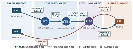
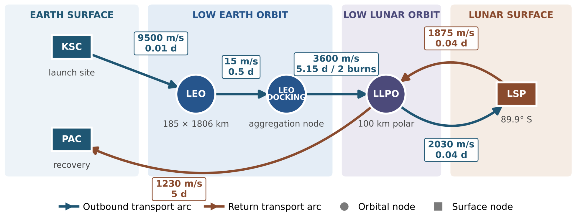
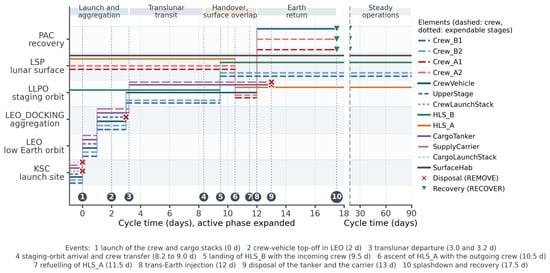
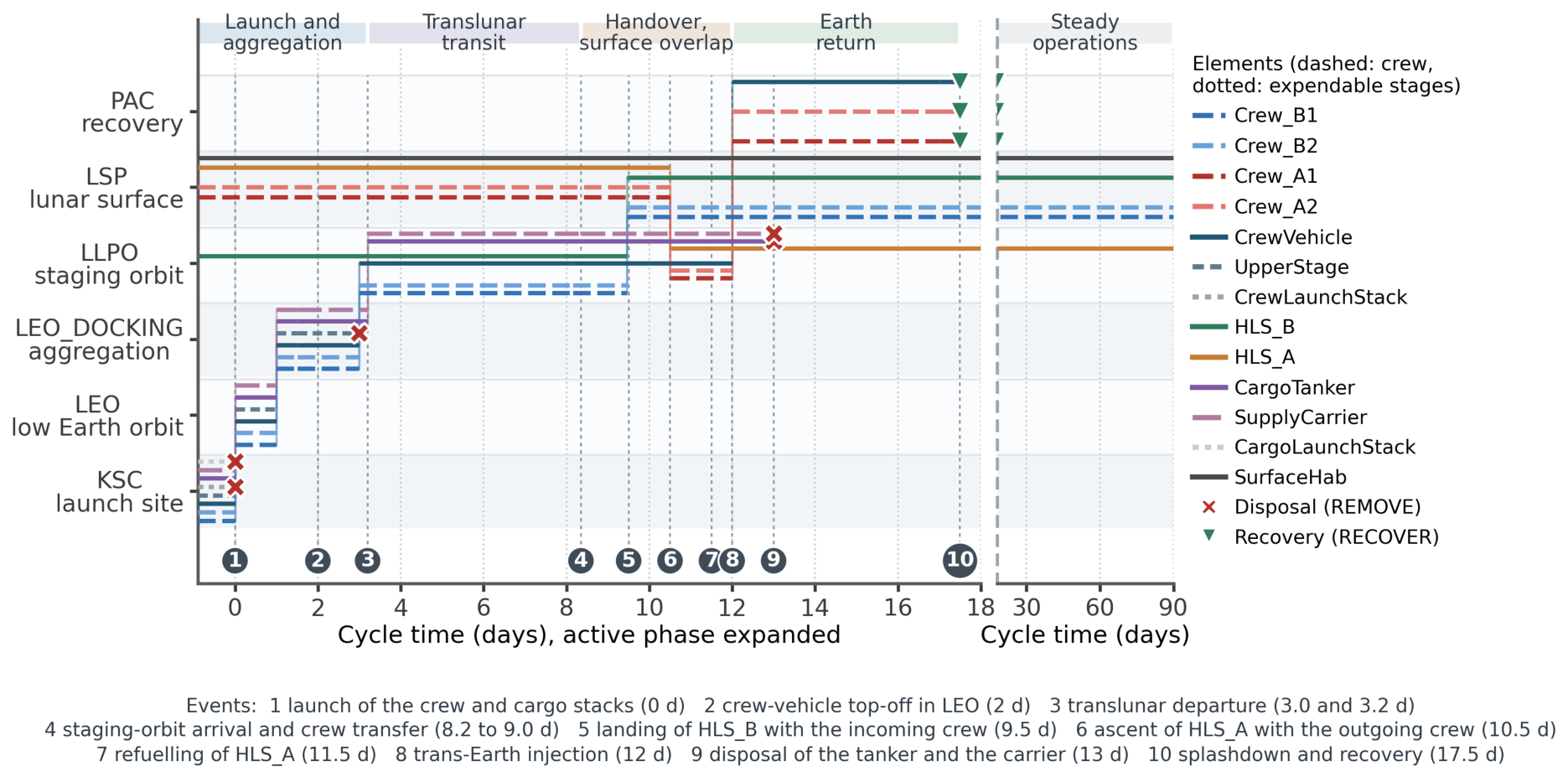
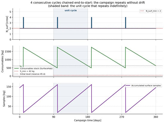
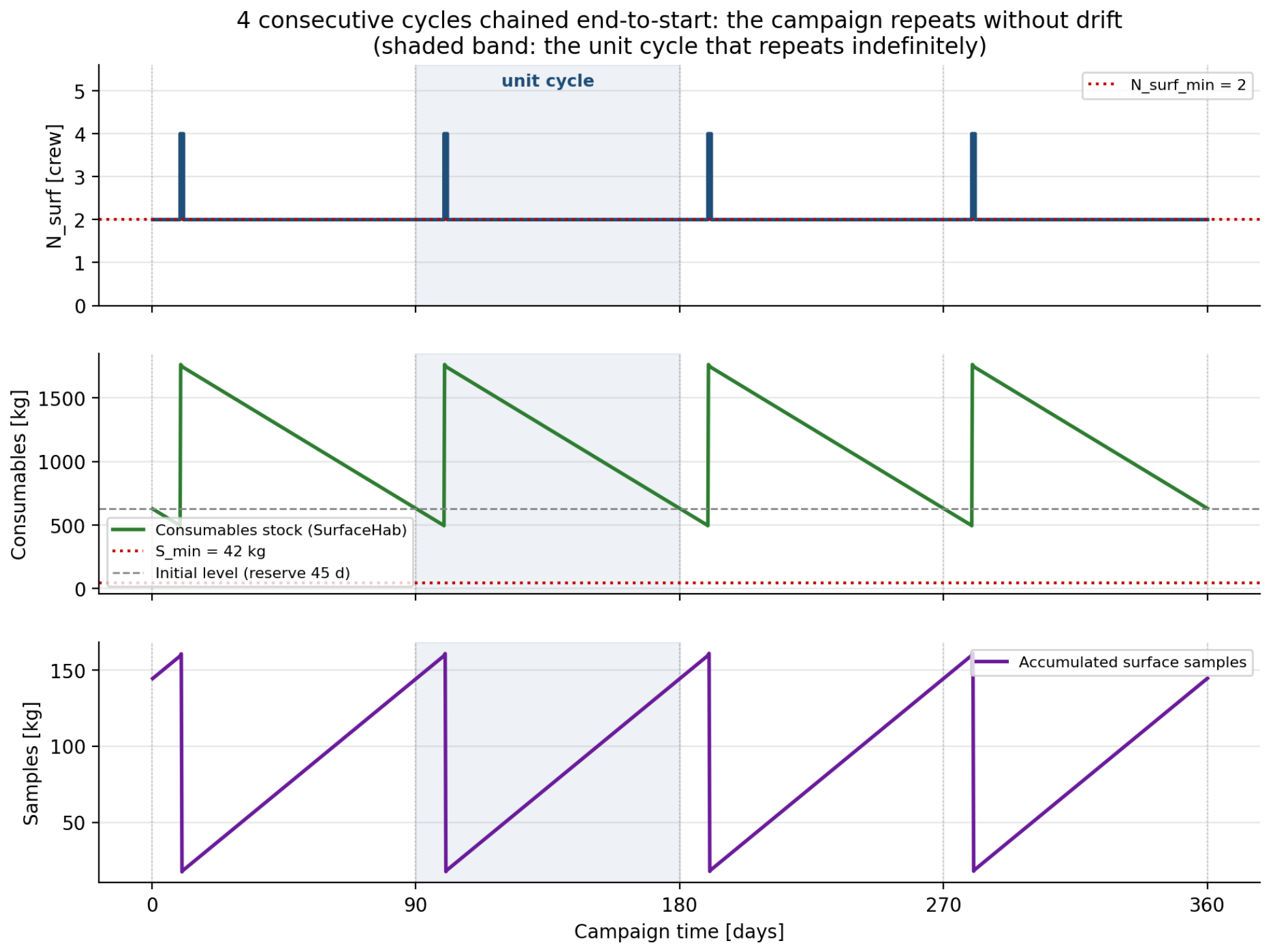
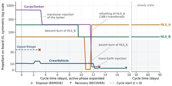
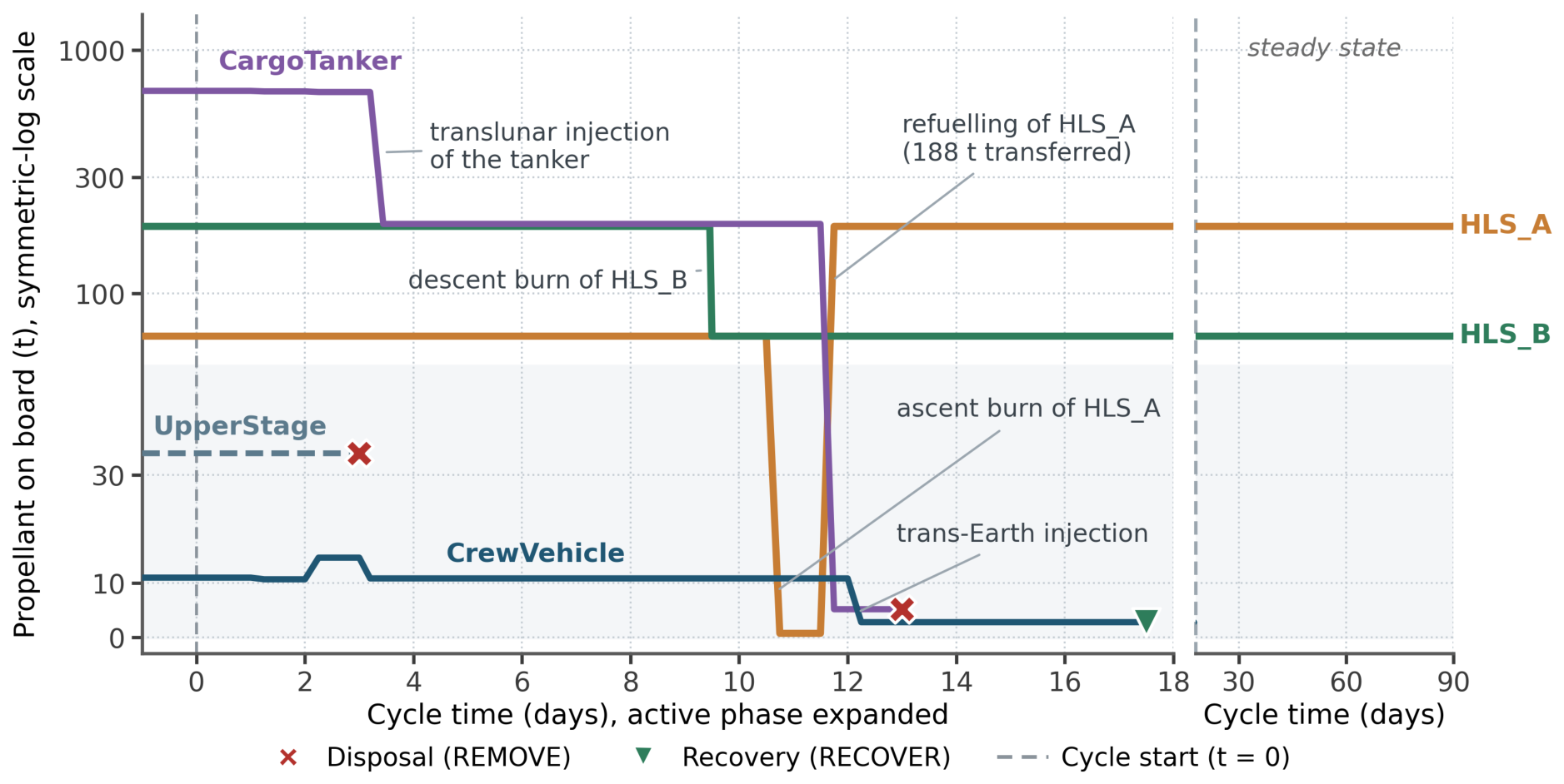
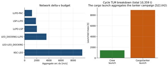
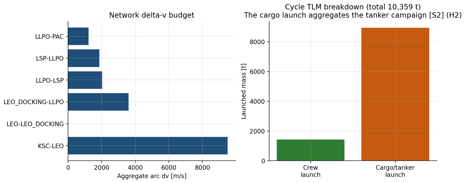
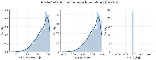
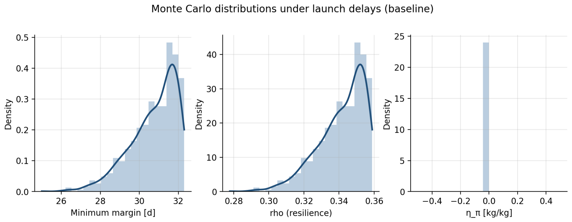
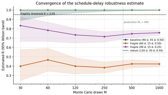
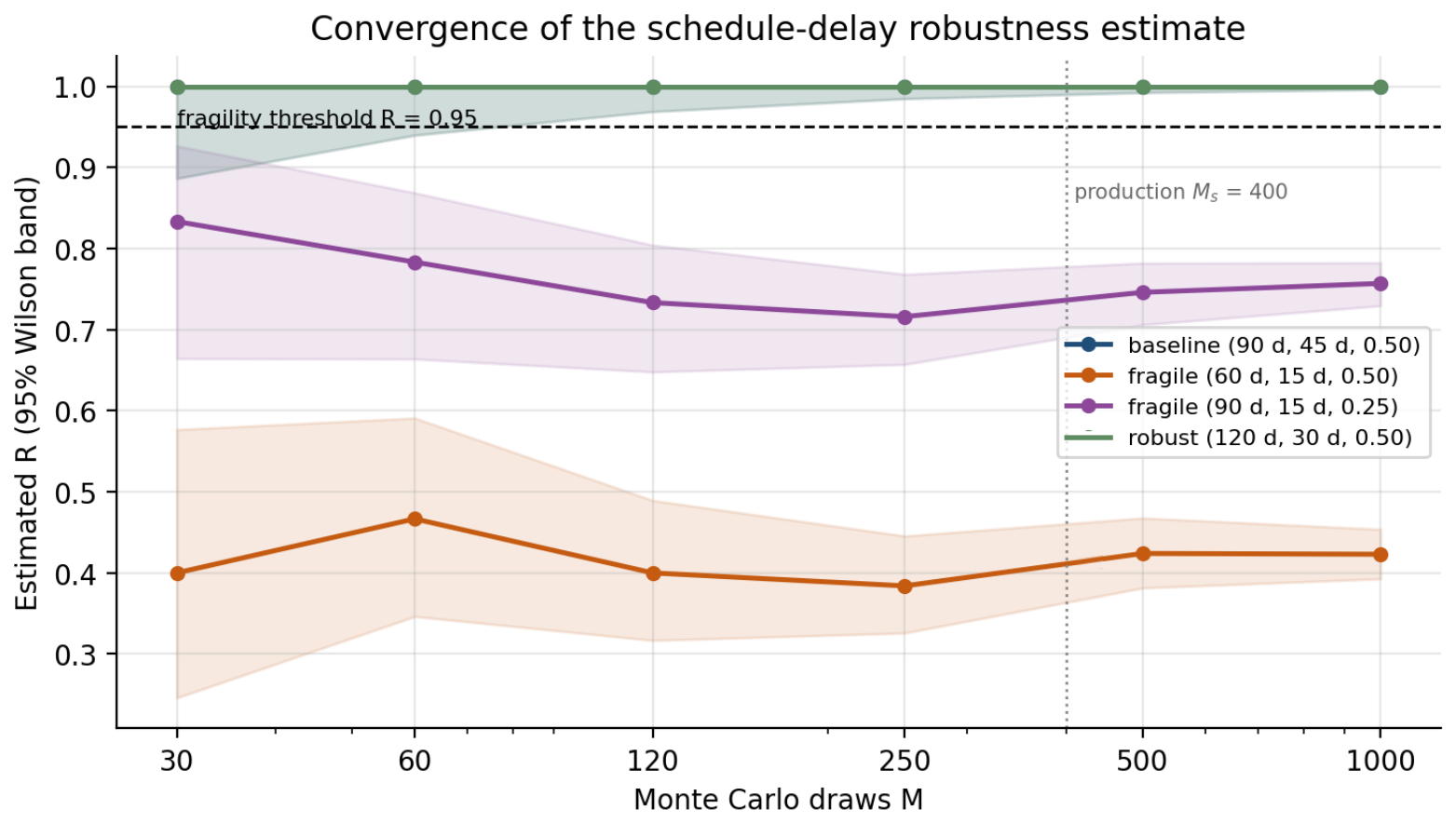
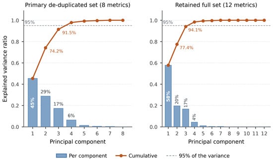
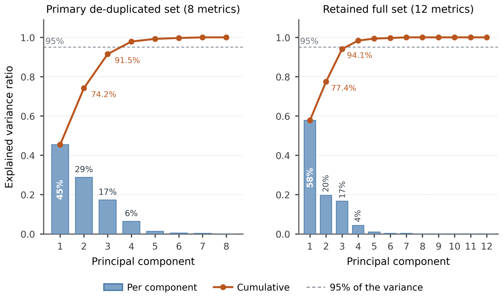
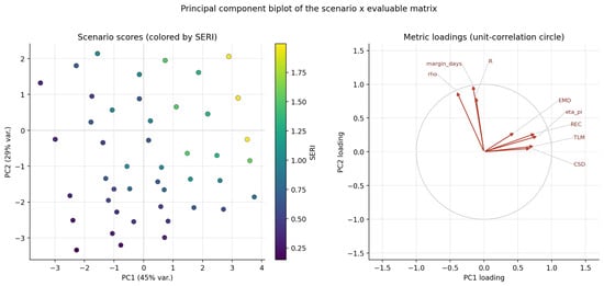
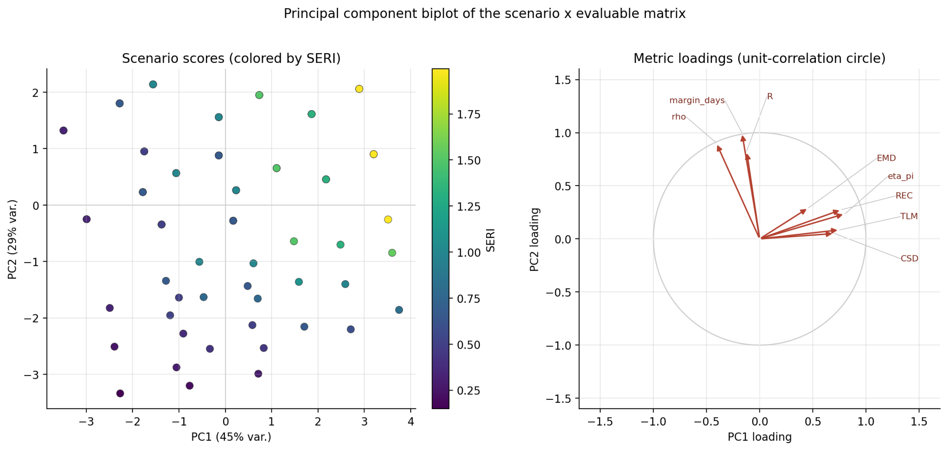
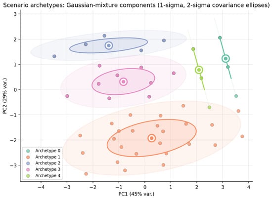
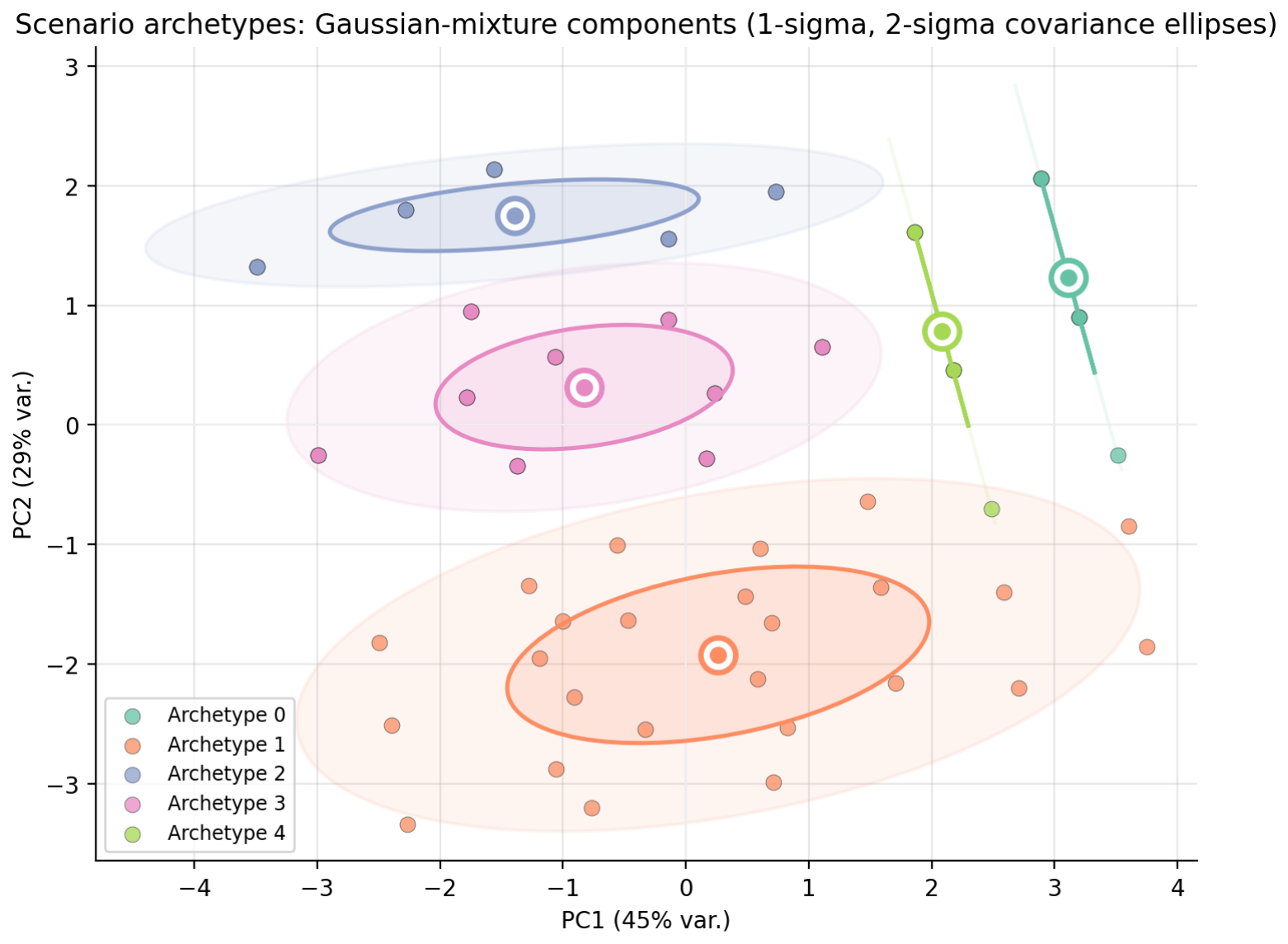
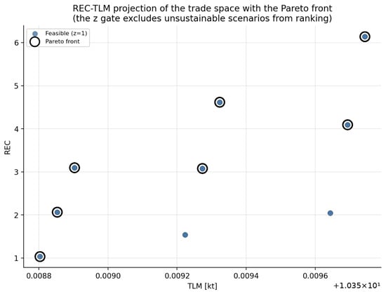
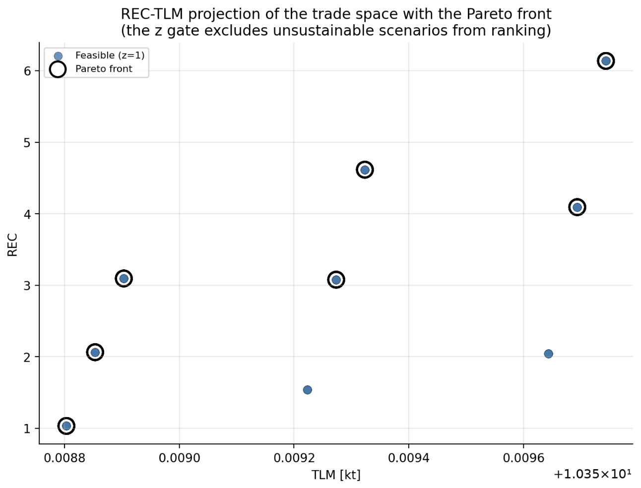
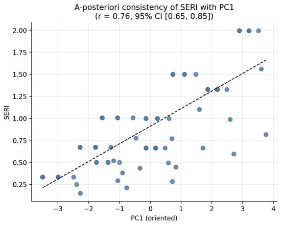
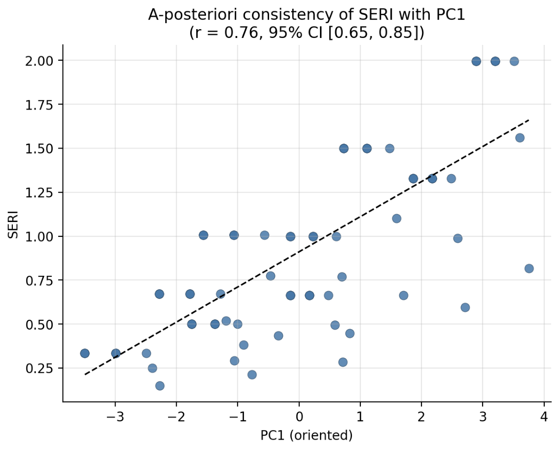
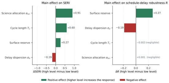
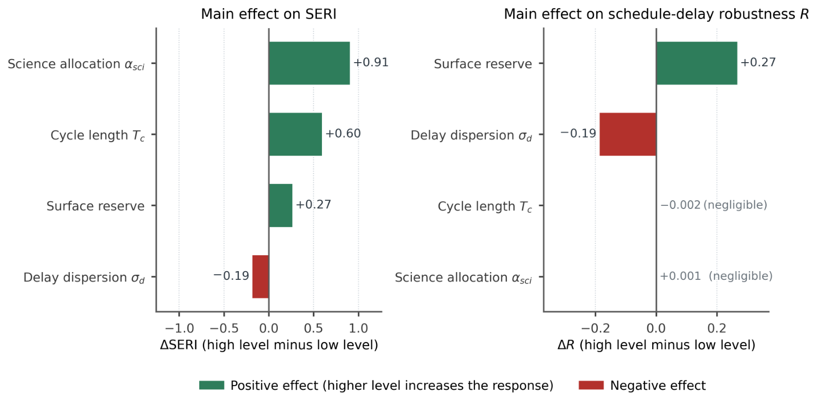
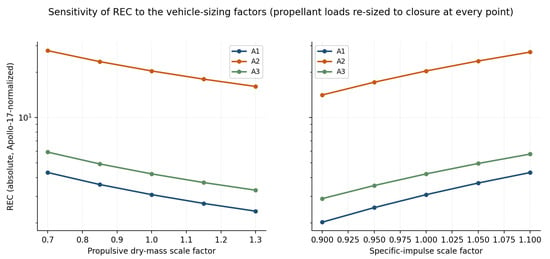
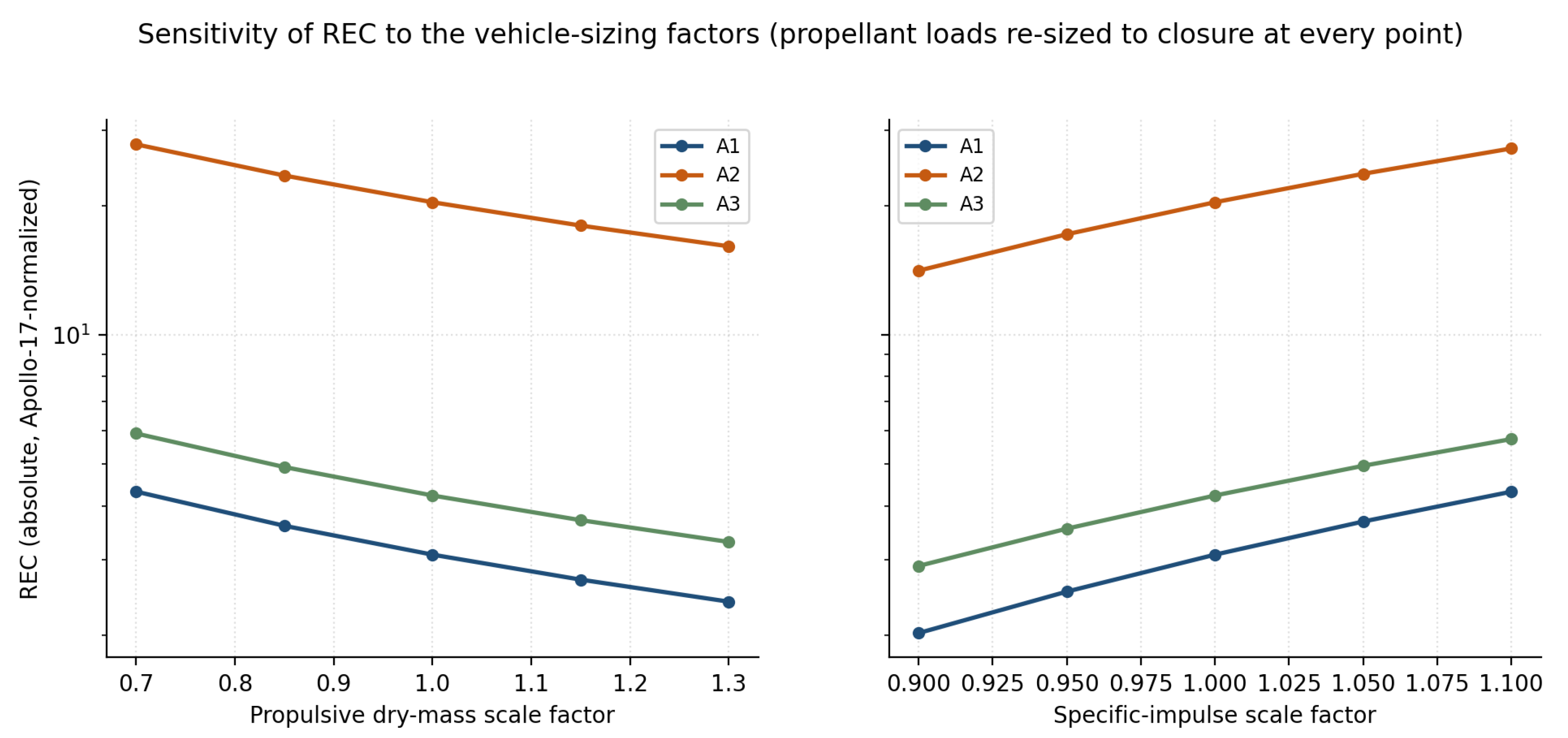
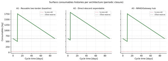
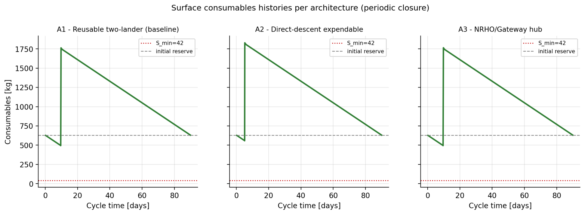
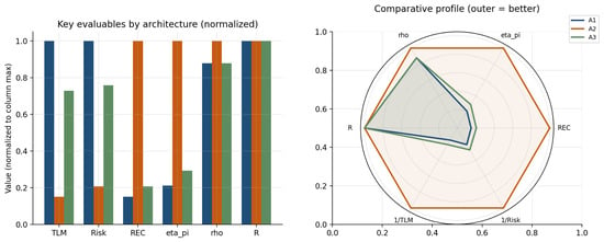
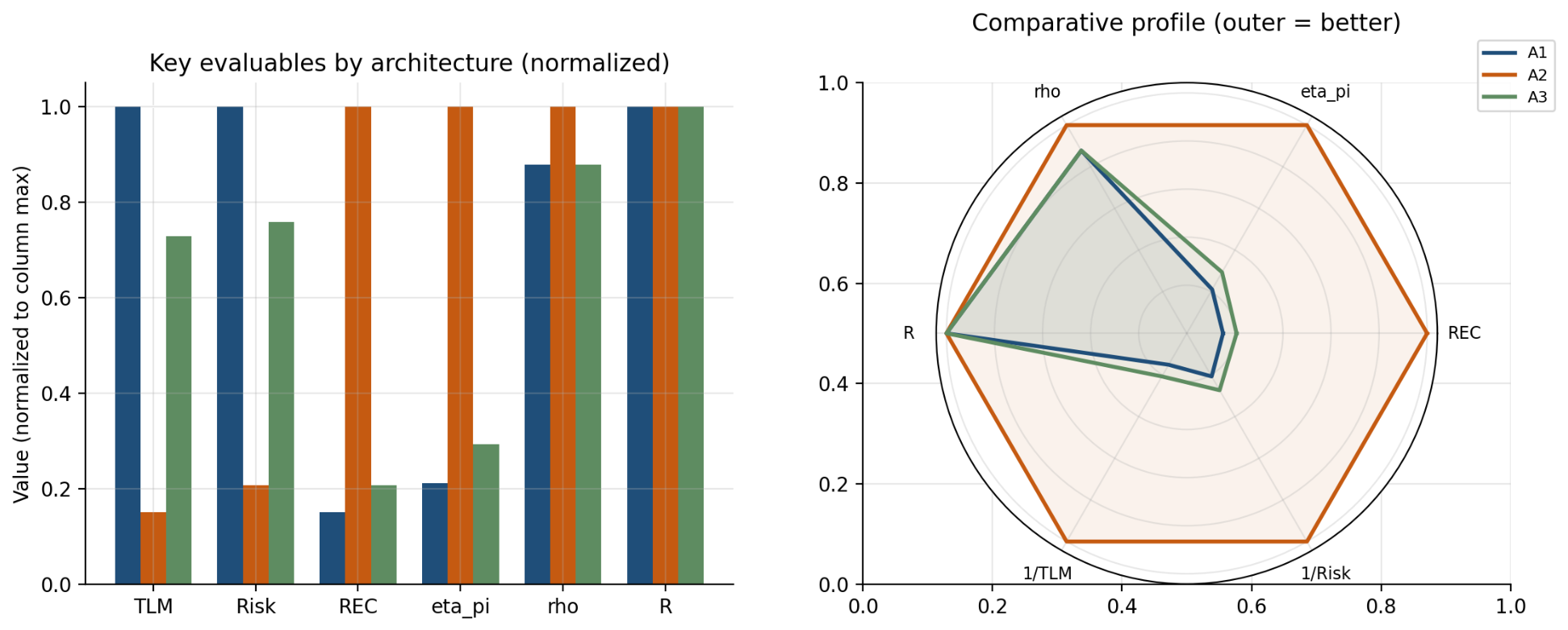
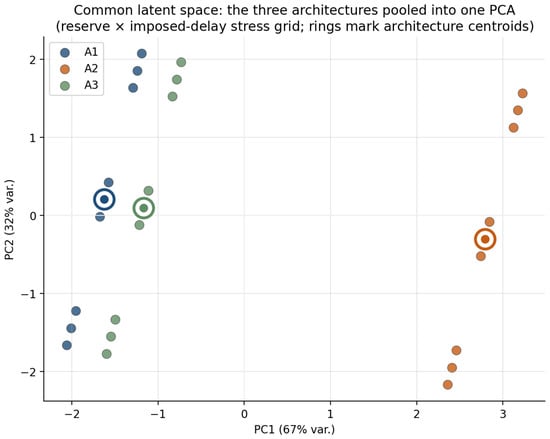
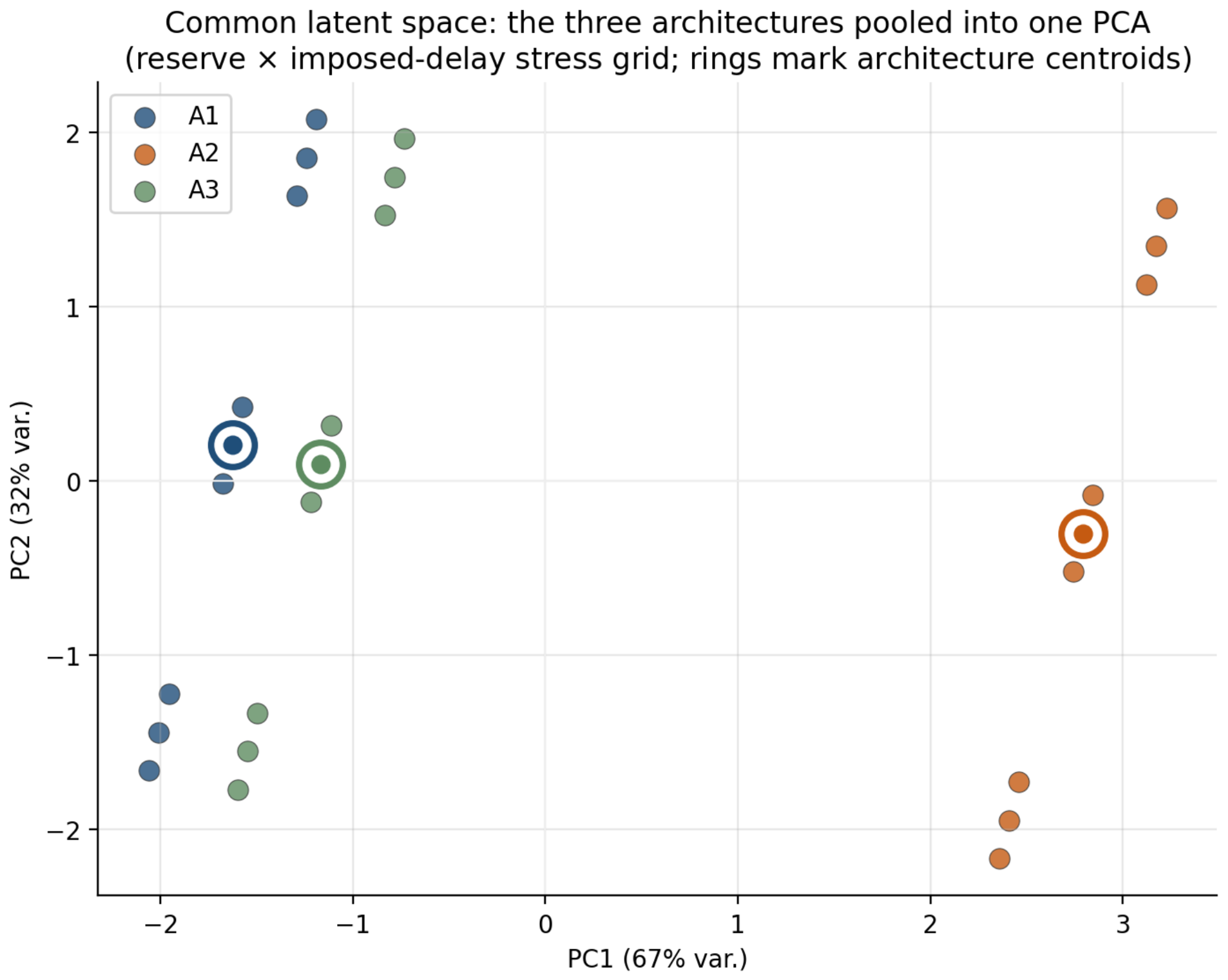

Disclaimer/Publisher’s Note: The statements, opinions and data contained in all publications are solely those of the individual author(s) and contributor(s) and not of MDPI and/or the editor(s). MDPI and/or the editor(s) disclaim responsibility for any injury to people or property resulting from any ideas, methods, instructions or products referred to in the content. |
© 2026 by the authors. Licensee MDPI, Basel, Switzerland. This article is an open access article distributed under the terms and conditions of the Creative Commons Attribution (CC BY) license.