Multi-History-Weighted Projection-Adaptive Jacobian Control for Close-Range UAV Visual Servoing near Overhead Ground Wires

Abstract

Close-range UAV visual servoing near overhead ground wires requires simultaneous regulation of the target’s lateral position, apparent width, and orientation angle in the image. Owing to flight-control response lag and visual-processing delay, current image changes may reflect the combined effects of multiple historical control inputs. To address this issue, this paper proposes a multi-history-weighted projection-adaptive Jacobian control method (MHW-PAJ-CLF). For each visual channel, the method takes a weighted sum of the parameter corrections associated with different historical inputs based on response prediction errors and input magnitudes and updates the local Jacobian matrix online under projection bounds. The online estimate is then blended with the nominal model. Control Lyapunov function-based quadratic programming (CLF-QP) uses the blended model to generate velocity and yaw-rate commands, coordinating the regulation of the three visual errors under input constraints. Comparative experiments were conducted on the RflySim–PX4 hardware-in-the-loop platform. The proposed method achieves a mean success rate of 75.50%, exceeding that of the best baseline by 11.05 percentage points. In tests with additional visual-feedback delay and command–response lag, the proposed method achieves lower overall tracking error than single-history PAJ-CLF, indicating that multi-history weighting helps improve visual tracking under time delays.

1. Introduction

Overhead ground wires are key components of lightning-protection systems for transmission lines, and their operating conditions directly affect transmission-line safety and power-supply reliability. Compared with manual inspection, UAV-based inspection can reduce risks to personnel during high-voltage and long-distance operations and improve inspection efficiency. Existing work on UAV-based power-line inspection covers inspection methods and engineering challenges [1], visual assistance for inspection and landing [2], UAV-LiDAR-based intelligent inspection [3], perception-aware control for line inspection [4], and multi-UAV cooperative inspection and maintenance [5]. However, close-range visual servoing near an overhead ground wire differs from conventional waypoint tracking. The UAV must maintain a line-shaped target within the camera field of view while simultaneously regulating its lateral position, apparent width, and orientation angle. In ultra-high-voltage electromagnetic environments, external positioning information or relative-range measurements may be unreliable, making close-range visual servoing more dependent on onboard visual measurements. Image sampling, target detection, filtering, and actuation jointly introduce a temporal lag between control input and visual response. This paper investigates coordinated regulation of multidimensional image errors under this temporal lag in close-range visual servoing near overhead ground wires.

Reliable extraction of the line target is the prerequisite for this task. Zhang et al. proposed an attention-guided multitask network for power-line component detection [6]. Liu et al. developed a deep-learning framework for key-target and defect detection on high-voltage transmission lines [7]. Choudhary et al. designed a lightweight detector for power-line components in UAV images [8]. Xu et al. improved orientation representation for rotated targets through instance-level orientation enhancement [9]. These advances provide the image measurements required for close-range control, but the detected line features must still be converted into coordinated flight commands. Beyond perception alone, Lin and Lai integrated YOLO-based runway detection and CNN-based localization with guidance and flight-control laws for fixed-wing UAV landing in GNSS-denied environments [10].

Image-based visual servoing (IBVS) generates motion commands directly from image-feature errors and therefore reduces dependence on complete three-dimensional reconstruction. Wang et al. extended IBVS to quadrotors tracking arbitrary flight targets [11]. Li et al. developed a robocentric model-based visual-servoing framework for quadrotor flight [12]. Xie et al. constructed a UAV visual-servoing controller using a virtual camera to accommodate changes in system parameters [13]. Lin et al. introduced robust observer-based visual control for tracking unknown moving targets [14]. Image-based feedback has also been applied to moving-platform landing and planar-target tracking [15,16]. Yang et al. combined IBVS with delayed state estimation for high-speed multicopter interception [17]. For measurement delay caused by image acquisition and processing, Yang et al. developed a sampled-data visual-servoing method using a time-delay disturbance observer [18]. Chen et al. addressed unmeasured states and disturbances through robust observation and output feedback [19]. Sepahvand et al. employed a self-organizing neural network to compensate for uncertainty in aerial-robot IBVS [20]. These studies cover target-relative flight in tracking, interception, and landing tasks. Close-range line tracking also requires the local mapping error from control commands to image variation to be addressed.

Constraint-aware, predictive, and learning-based methods have been introduced to improve visual-control performance. Yang and Li incorporated visibility constraints into robust model predictive visual servoing [21]. Zhou et al. combined constrained IBVS with sampling-based planning to handle image and physical constraints [22]. Liu et al. developed a dual-rate predictive observer for low camera-sampling rates and view constraints [23]. Yi et al. used a neural network to compensate for model uncertainty in quadrotor IBVS [24]. More recently, Byun et al. proposed vector-field-based robust landing on a moving platform [25]. Zhang et al. developed data-driven generalized iterative predictive control for nonlinear and coupled UAV dynamics [26]. Guo et al. addressed image-based formation encirclement and tracking of unknown targets [27]. These methods improve visibility maintenance, predictive regulation, and uncertainty compensation. Updating the local image-response model also requires relating the observed image changes to the earlier commands that produced them.

Online estimation offers a complementary means of reducing local model mismatch. Pan and Shi incorporated online data memory into adaptive estimation and control [28]. Li et al. used stored data in composite learning for uncalibrated visual servoing [29]. Kamath and Feroskhan mapped image variations directly to multirotor input commands through augmented dynamics [30]. Kamath et al. subsequently introduced a physics-informed Koopman neural operator for augmented-dynamics visual servoing [31]. These methods use closed-loop data to update the mapping between control input and image response. A projection-adaptive Jacobian (PAJ) update provides a lightweight online correction of the local image-response matrix. The PAJ baseline uses the current image-state change and a single recent control input to update the model. Flight-control response, actuation, and visual processing take time. The current image change may therefore reflect several earlier commands. The relevant input history can vary with the command response and visual channel.

The proposed multi-history-weighted projection-adaptive Jacobian method uses CLF-QP command generation and is termed MHW-PAJ-CLF. For each visual channel, the current model predicts the response to each historical input. Comparing each prediction with the observed state-change rate gives its response error. These errors and the input magnitudes determine the weights used to sum the PAJ parameter corrections. The update includes a correction toward the nominal value, and projection bounds the result. The updated estimate and the nominal model are combined in a prescribed proportion. The CLF-QP uses this model to regulate the three visual errors within the velocity and yaw-rate limits. The main contributions are as follows:

• A multi-history-weighted projection-adaptive Jacobian update method is proposed to address flight-control response lag and visual-processing delay. For each visual channel, parameter corrections associated with multiple historical inputs are weighted and summed according to response prediction errors and input magnitudes to update the local image-response model online.
• A three-channel visual-servoing framework is developed for close-range operations near overhead ground wires. The online Jacobian estimate is blended with the nominal model and used by the CLF-QP to coordinate regulation of the target’s lateral position, apparent width, and orientation angle within the velocity and yaw-rate limits.
• Comparative experiments are conducted on the RflySim–PX4 hardware-in-the-loop platform. The results show that the proposed method achieves better overall visual tracking performance than the comparison baselines, with lower mean absolute visual errors and a higher mean success rate.

2. System Modeling

This section first establishes the UAV dynamic model, then defines the visual errors of the overhead ground wire, and, finally, describes the local relationship between the control input and visual-error variation.

2.1. UAV Modeling

The UAV dynamics are described by a six-degree-of-freedom rigid-body model. The NED frame is used as the inertial frame $\mathcal{I}$, and the FRD frame is used as the body frame $\mathcal{B}$, where $x_b$, $y_b$, and $z_b$ point forward, rightward, and downward, respectively. The UAV position and velocity are expressed in the NED frame as

$${\mathit{p}}_u={[x,y,z]}^{\mathrm{T}},$$

(1)

$$\mathit{v}={[v_x,v_y,v_z]}^{\mathrm{T}}.$$

(2)

The attitude is described by the rotation matrix $\mathit{R}\in SO\left(3\right)$, which transforms vectors from the body frame $\mathcal{B}$ to the NED frame $\mathcal{I}$. The body-frame angular velocity is

$$\mathit{\omega }={[p,q,r]}^{\mathrm{T}}.$$

(3)

The translational and rotational dynamics are

$${\dot{\mathit{p}}}_u=\mathit{v},$$

(4)

$$m\dot{\mathit{v}}=\left[\begin{array}{c}0\\ 0\\ mg\end{array}\right]+\mathit{R}\left[\begin{array}{c}0\\ 0\\ -T\end{array}\right]+{\mathit{f}}_d,$$

(5)

$$\dot{\mathit{R}}=\mathit{R}{\left[\mathit{\omega }\right]}_{\times },$$

(6)

$$\mathit{J}\dot{\mathit{\omega }}=\mathit{\tau }-\mathit{\omega }\times \mathit{J}\mathit{\omega }+{\mathit{\tau }}_d,$$

(7)

where m is the UAV mass, $\mathit{J}$ is the inertia matrix, g is the gravitational acceleration, and ${\mathit{f}}_d$ and ${\mathit{\tau }}_d$ denote aerodynamic drag, modeling errors, and external disturbances. The total thrust T and body-frame control torque $\mathit{\tau }={[{\tau }_x,{\tau }_y,{\tau }_z]}^{\mathrm{T}}$ are obtained by summing the contributions of the four rotors:

$$T={\displaystyle \sum _{i=1}^4}{T}_i,$$

(8)

$$\mathit{\tau }={\displaystyle \sum _{i=1}^4}\left({\mathit{r}}_i\times \left[\begin{array}{c}0\\ 0\\ -T_i\end{array}\right]+\left[\begin{array}{c}0\\ 0\\ M_i\end{array}\right]\right),$$

(9)

where $T_i$ and $M_i$ are the thrust and reaction torque generated by the ith rotor, respectively, and ${\mathit{r}}_i$ is its body-frame position vector relative to the vehicle center of mass. For the ith rotor with angular speed ${\mathrm{\Omega }}_i$, $T_i$ and $M_i$ satisfy the quadratic relations

$$T_i=k_T{\mathrm{\Omega }}_i^2,$$

(10)

$$M_i={\sigma }_i{k}_M{\mathrm{\Omega }}_i^2,$$

(11)

where $k_T$ and $k_M$ are the thrust and reaction-torque coefficients, respectively, and ${\sigma }_i\in \{+1,-1\}$ denotes the rotor rotation direction. The motor response is approximated by a first-order lag:

$$\begin{array}{c}{\dot{\mathrm{\Omega }}}_i={\displaystyle \frac{1}{{\tau }_m}}({\mathrm{\Omega }}_{i,\mathrm{ss}}-{\mathrm{\Omega }}_i),\\ {\mathrm{\Omega }}_{i,\mathrm{ss}}=a_{\mathrm{\Omega }}{u}_{m,i}+b_{\mathrm{\Omega }}\end{array},$$

(12)

where ${\mathrm{\Omega }}_{i,\mathrm{ss}}$ is the steady-state motor speed corresponding to $u_{m,i}$, $u_{m,i}$ is the normalized motor-throttle command generated by the mixer, $a_{\mathrm{\Omega }}$ and $b_{\mathrm{\Omega }}$ are the slope and intercept of the steady-state throttle–speed relation, and ${\tau }_m$ is the motor response time constant.

2.2. Visual-Error Modeling

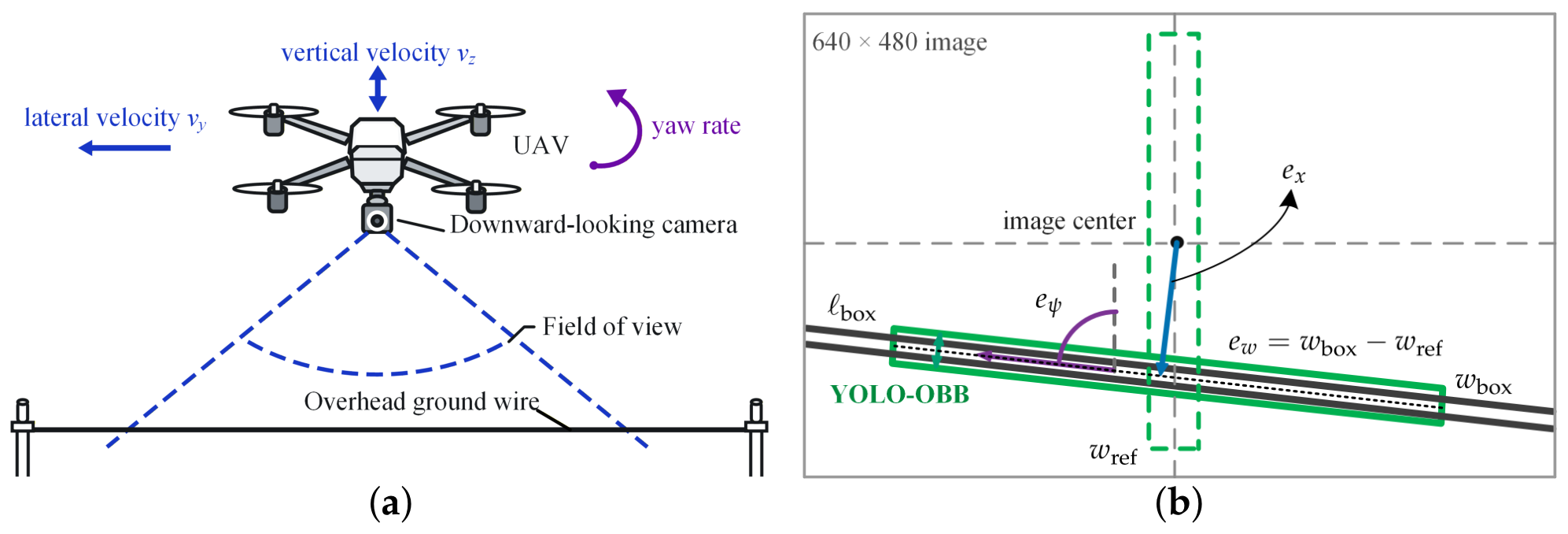
The YOLO11s-OBB detector provides the rotated bounding box of the overhead ground wire. Its centerline position, short-side width, and orientation angle define the three image-space quantities used for visual regulation, as illustrated in Figure 1b.

As shown in Figure 1b, the green solid box denotes the current rotated bounding box of the overhead ground wire detected by YOLO11s-OBB, and the green dashed box denotes the desired target box. The two dark-gray parallel lines denote the image boundaries of the same overhead ground wire. Let the image center be $c_{\mathrm{img}}$, the centerline of the current detection box be ${𝓁}_{\mathrm{box}}$, the short-side width of the detection box be $w_{\mathrm{box}}$, and the box orientation angle be ${\psi }_{\mathrm{box}}$. With desired box width $w_{\mathrm{ref}}$ and orientation angle ${\psi }_{\mathrm{ref}}$, the raw visual-error vector is

$$\mathit{e}={\left[\begin{array}{ccc}{e}_x& e_w& e_{\psi }\end{array}\right]}^{\mathrm{T}},$$

(13)

where $e_x$ is the lateral-position error between the image center and the target-box centerline, $e_w=w_{\mathrm{box}}-w_{\mathrm{ref}}$ is the apparent-width error, and $e_{\psi }$ is the angle error between the detected and desired box orientation angles.

Before $e_{\psi }$ is calculated, the detected box orientation is mapped to $[-\pi /2,\pi /2)$. When the angle crosses an interval boundary, equivalent wire orientations separated by $\pi$ are used to correct angle jumps between successive frames.

Within the local regulation region, when the UAV is approximately level and the wire is near the center of the downward-looking image, the apparent wire width increases as the camera–wire distance decreases. It therefore provides visual feedback for regulating the UAV’s vertical position relative to the wire.

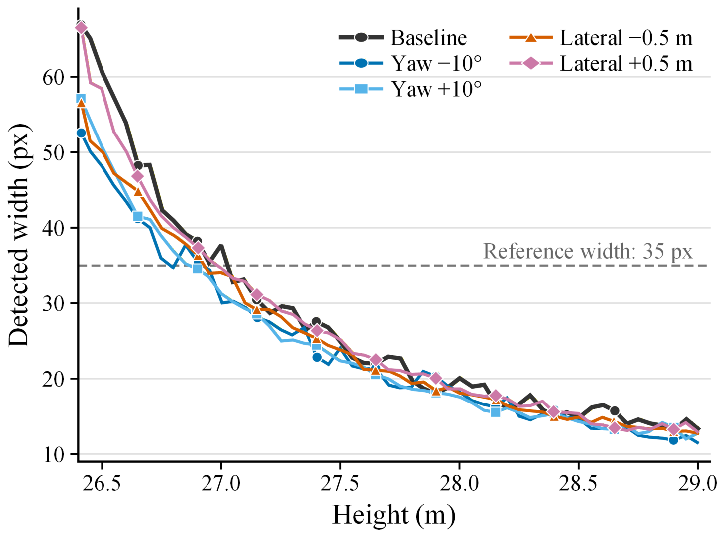
As shown in Figure 1a, flight height h and wire height $h_{\mathrm{w}}$ share the same height reference. When the UAV is approximately level and the wire is near the center of the downward-looking image, the camera–wire distance is approximately $h-h_{\mathrm{w}}$. Camera attitude and viewing direction also affect the apparent width. Calibration was performed during descent at the reference viewpoint, relative yaw offsets of $\pm {10}^{\circ }$, and lateral offsets of $\pm 0.5$ m, with flight height and detected short-side width recorded together (Figure 2). The desired width is set to $w_{\mathrm{ref}}=35\mathrm{px}$.

2.3. Three-Channel Visual State and Control Input

Because the lateral-position, apparent-width, and angle errors have different physical dimensions and numerical scales, the normalized three-channel visual state is defined to balance the relative contributions of the three channels:

$$\mathit{q}={\left[\begin{array}{ccc}{e}_x/s_x& e_w/s_w& e_{\psi }/s_{\psi }\end{array}\right]}^{\mathrm{T}},$$

(14)

where $s_x$, $s_w$, and $s_{\psi }$ are the normalization scales for the lateral-position, apparent-width, and angle errors, respectively. Let

$$\mathit{S}=\mathrm{diag}(s_x,s_w,s_{\psi }).$$

(15)

The normalized visual state can then be written as

$$\mathit{q}={\mathit{S}}^{-1}\mathit{e}.$$

(16)

If ${\mathit{B}}_e\left(t\right)$ denotes the local image-response matrix in the raw-error coordinates, its expression in the normalized visual-state coordinates is

$$\mathit{B}\left(t\right)={\mathit{S}}^{-1}{\mathit{B}}_e\left(t\right).$$

(17)

Therefore, the local image-response matrix $\mathit{B}\left(t\right)$, the online estimate $\widehat{\mathit{B}}$, and the nominal matrix ${\mathit{B}}_0$ are all defined in the same normalized visual-state coordinates.

The UAV control input is defined as

$$\mathit{u}={\left[\begin{array}{ccc}{v}_y^{\mathrm{ref}}& v_z^{\mathrm{ref}}& r^{\mathrm{ref}}\end{array}\right]}^{\mathrm{T}},$$

(18)

where $v_y^{\mathrm{ref}}$, $v_z^{\mathrm{ref}}$, and $r^{\mathrm{ref}}$ denote the lateral-velocity, vertical-velocity, and yaw-rate reference commands, respectively. The velocity reference commands use the body FRD frame. The three command channels predominantly regulate lateral image alignment, camera–wire distance represented by apparent width, and relative heading represented by the angle.

2.4. Local Image-Response Model

Within the current visual-regulation region, the relationship between the control input and the normalized visual-state rate is locally approximated as

$$\dot{\mathit{q}}=\mathit{B}\left(t\right)\mathit{u}+\mathit{\eta }\left(t\right),$$

(19)

where $\mathit{B}\left(t\right)$ is the local image-response matrix in normalized visual-state coordinates and describes the local effect of the control input $\mathit{u}$ on the visual-state rate $\dot{\mathit{q}}$. The term $\mathit{\eta }\left(t\right)$ collects the effects of detection noise, visual filtering, unmodeled dynamics, and other disturbances.

According to the dominant correspondences between lateral velocity, vertical velocity, and yaw rate and the three visual states, the local image-response matrix is decomposed as

$$\mathit{B}\left(t\right)={\mathit{B}}_d\left(t\right)+{\mathit{B}}_o\left(t\right),$$

(20)

where the diagonal component is defined as

$${\mathit{B}}_d\left(t\right)=\mathrm{diag}\left(B_{11}\left(t\right),B_{22}\left(t\right),B_{33}\left(t\right)\right)$$

(21)

The matrix ${\mathit{B}}_d\left(t\right)$ contains the three dominant channels, whereas ${\mathit{B}}_o\left(t\right)$ contains the off-diagonal coupling terms between channels. Equation (19) can therefore be rewritten as

$$\dot{\mathit{q}}={\mathit{B}}_d\left(t\right)\mathit{u}+{\mathit{\eta }}_o\left(t\right),$$

(22)

where ${\mathit{\eta }}_o\left(t\right)={\mathit{B}}_o\left(t\right)\mathit{u}+\mathit{\eta }\left(t\right)$ represents the off-diagonal channel response and other unmodeled terms.

Command transmission, flight-control response, actuation, and visual processing take time. The change between two visual frames may therefore reflect several earlier commands. This effect is expressed as

$${\mathit{q}}_k-{\mathit{q}}_{k-1}=T_{\mathrm{img},k}{\displaystyle \sum _{j=0}^{J_k}}{\mathit{H}}_k^{\left(j\right)}{\mathit{u}}_{k-1-j}+{\mathit{\zeta }}_k,$$

(23)

where $T_{\mathrm{img},k}=t_k-t_{k-1}$ is the interval between adjacent valid visual frames, $J_k$ is the currently available history depth, ${\mathit{H}}_k^{\left(j\right)}$ denotes the unknown linear contribution of the jth historical command to the current visual-state increment, and ${\mathit{\zeta }}_k$ represents the error outside the finite-history approximation.

Within the local visual-regulation region, each channel’s response gain is treated as approximately constant over the short history window. Each historical input in that channel is evaluated using the same current parameter estimate.

Equation (23) describes how several historical commands contribute to the current visual change. For online updating, each historical input is multiplied by the current gain estimate of its channel to obtain the corresponding prediction of the visual-state rate. The difference between each prediction and the observed rate is used to compute a PAJ parameter correction. These corrections are weighted and summed separately for each channel. Inter-channel effects, timing differences, and other dynamics are collected in the local-model error.

The model is initialized using the nominal local image-response matrix ${\mathit{B}}_0$:

$${\mathit{B}}_0=\left[\begin{array}{ccc}{b}_{11}& 0& 0\\ 0& b_{22}& 0\\ 0& 0& b_{33}\end{array}\right],$$

(24)

where $b_{11}$, $b_{22}$, and $b_{33}$ describe the locally dominant responses from the lateral-velocity, vertical-velocity, and yaw-rate commands to the three normalized visual-state channels, respectively. Each online update includes a correction toward ${\mathit{B}}_0$.The control model combines the updated estimate and ${\mathit{B}}_0$ in a prescribed proportion.

3. MHW-PAJ-CLF Control Method

3.1. Control Architecture

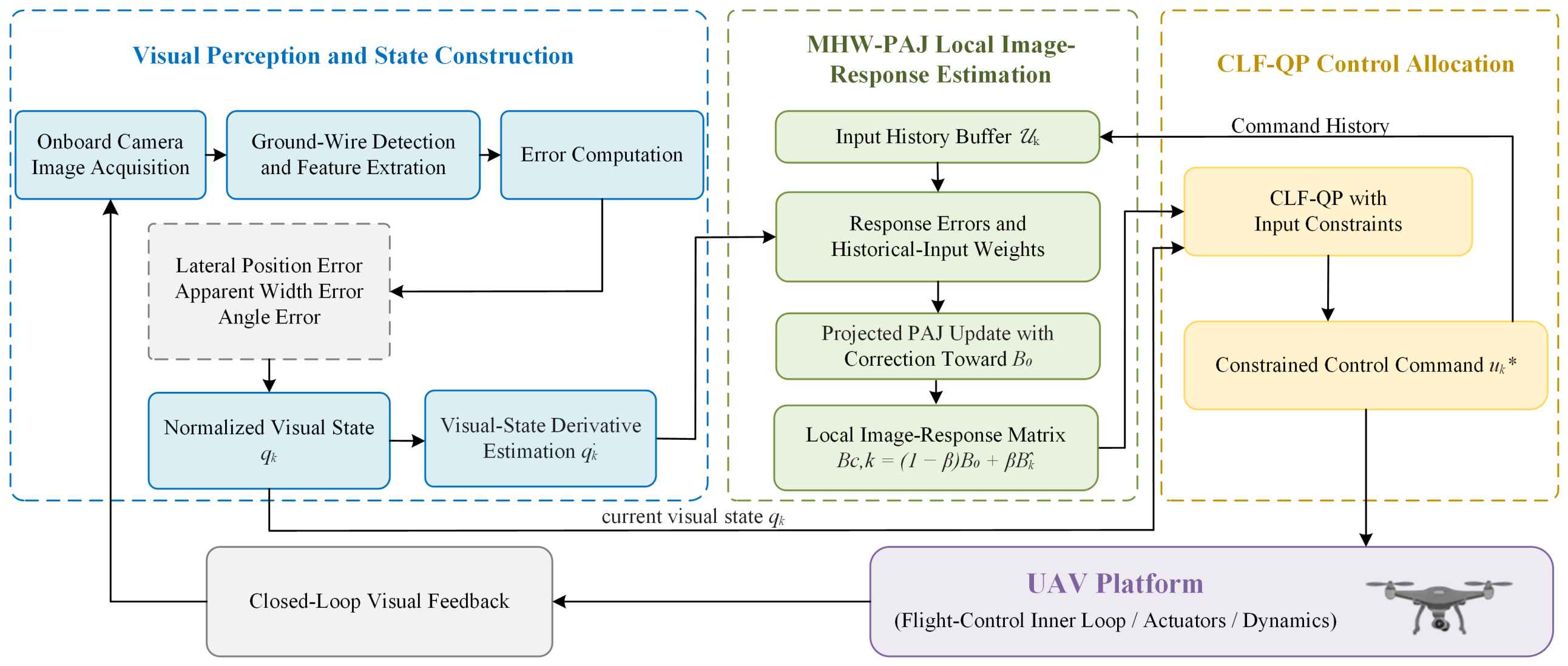
Figure 3 shows the MHW-PAJ-CLF control loop. At each valid visual update, the perception module forms ${\mathit{q}}_k$ from the three filtered visual errors. It estimates ${\dot{\mathit{q}}}_k$ from two consecutive valid states. MHW-PAJ uses each historical input in ${\mathcal{U}}_k$ to compute a response error and a PAJ parameter correction. For each channel, the corrections are weighted using the response errors and input magnitudes, then summed. The update includes a correction toward the nominal value, and projection bounds the result. The updated estimate and ${\mathit{B}}_0$ are combined in a prescribed proportion to obtain ${\mathit{B}}_{c,k}$. The CLF-QP uses ${\mathit{q}}_k$ and ${\mathit{B}}_{c,k}$ to compute ${\mathit{u}}_k^{\star }$ within the input limits. The command is sent to the UAV; at each valid visual update, the previous control input ${\mathit{u}}_{k-1}$ is used together with earlier inputs to update the model. A new valid visual frame triggers a parameter update. Between visual frames, the control loop computes commands using the latest visual state and model.

3.2. Conventional Projection-Adaptive Jacobian Update

The PAJ update uses the visual-state rate computed from two consecutive valid visual frames. For channel i, this rate is approximated as

$${\dot{q}}_{i,k}={\displaystyle \frac{q_{i,k}-q_{i,k-1}}{t_k-t_{k-1}}}={\displaystyle \frac{q_{i,k}-q_{i,k-1}}{T_{\mathrm{img},k}}},$$

(25)

where $T_{\mathrm{img},k}=t_k-t_{k-1}$ is the interval between adjacent valid visual frames and is used directly in the finite difference.

At each valid visual update, PAJ pairs ${\dot{q}}_{i,k}$ with the most recent historical control input $u_{i,k-1}$ and updates the local image-response parameter as

$${\widehat{\theta }}_{i,k}={\mathrm{\Pi }}_i\left[{\widehat{\theta }}_{i,k-1}+\gamma {\displaystyle \frac{u_{i,k-1}}{ϵ+u_{i,k-1}^2}}\left({\dot{q}}_{i,k}-{\widehat{\theta }}_{i,k-1}{u}_{i,k-1}\right)+\lambda T_{\mathrm{img},k}({\theta }_{0,i}-{\widehat{\theta }}_{i,k-1})\right],$$

(26)

where $\gamma >0$ is the adaptive gain that regulates online correction speed and sensitivity to measurement noise, $ϵ>0$ is the update regularizer that limits numerical amplification by small inputs, $\lambda \ge 0$ slowly moves the estimate toward its nominal value under weak excitation, and ${\theta }_{0,i}$ is the nominal response parameter of channel i. The projection operator ${\mathrm{\Pi }}_i$ restricts the updated estimate to $[{\underline{\theta }}_i,{\overline{\theta }}_i]$, thereby ensuring bounded online estimates. The denominator $ϵ+u_{i,k-1}^2$ scales the correction of channel i using the corresponding channel-input energy.

3.3. Multi-History-Weighted Projection-Adaptive Jacobian Update

The current visual change may reflect several historical commands. MHW-PAJ uses the current parameter estimate to predict the state-change rate for each historical input. It compares these predictions with the observed rate and assigns weights using the response errors and input magnitudes.

At the kth valid visual update, the control-input history is written as

$${\mathcal{U}}_k=\{{\mathit{u}}_{k-1},{\mathit{u}}_{k-2},\dots ,{\mathit{u}}_{k-1-N_d}\},$$

(27)

where $N_d$ is the maximum history-buffer depth, $J_k\le N_d$ is the largest currently available history lag, and $j=0,\dots ,J_k$ denotes the lag, in visual-update steps, of a historical input relative to the current update.

For channel $i\in \{1,2,3\}$, the input magnitudes within the history window are checked first. Let $u_{\mathrm{th}}>0$ be the prescribed excitation-level parameter, with the channel threshold set to $u_{\mathrm{th}}/\sqrt{3}$. If

$$\underset{0\le j\le J_k}{\max }\left|u_{i,k-1-j}\right|<{\displaystyle \frac{u_{\mathrm{th}}}{\sqrt{3}}},$$

the response-error correction of channel i is set to zero, and the $\lambda$ term in Equation (34) moves the estimate toward the nominal value before projection is applied. Otherwise, the response error and weight associated with each historical input are calculated. The response error for the jth historical input is defined as

$$r_{i,k}^{\left(j\right)}={\dot{q}}_{i,k}-{\widehat{\theta }}_{i,k-1}{u}_{i,k-1-j},$$

(28)

where $r_{i,k}^{\left(j\right)}$ is the difference between the observed state-change rate and the prediction for the jth historical input. All predictions for channel i use the same estimate ${\widehat{\theta }}_{i,k-1}$. The response errors are scaled within each channel using

$${\sigma }_{i,k}^2={\displaystyle \frac{1}{J_k+1}}{\displaystyle \sum _{j=0}^{J_k}}{\left(r_{i,k}^{\left(j\right)}\right)}^2+{ϵ}_r,$$

(29)

where ${ϵ}_r>0$ is the error-scale regularizer. The input-magnitude factor is defined as

$${\chi }_{i,k}^{\left(j\right)}={\displaystyle \frac{u_{i,k-1-j}^2}{{ϵ}_u+u_{i,k-1-j}^2}},$$

(30)

where ${ϵ}_u>0$ is a regularizer; ${\chi }_{i,k}^{\left(j\right)}$ approaches unity as the input magnitude increases.

The historical-input weights are defined by the response error and input magnitude as

$$\begin{array}{cc}\hfill {\tilde{w}}_{i,k}^{\left(j\right)}& ={\chi }_{i,k}^{\left(j\right)}\exp \left[-{\displaystyle \frac{{\left(r_{i,k}^{\left(j\right)}\right)}^2}{{\sigma }_{i,k}^2}}\right],\hfill \end{array}$$

(31)

$$\begin{array}{cc}\hfill w_{i,k}^{\left(j\right)}& ={\displaystyle \frac{{\tilde{w}}_{i,k}^{\left(j\right)}}{{\sum }_{𝓁=0}^{J_k}{\tilde{w}}_{i,k}^{(𝓁)}}},\hfill \end{array}$$

(32)

where ${\tilde{w}}_{i,k}^{\left(j\right)}$ and $w_{i,k}^{\left(j\right)}$ are the unnormalized and normalized weights, respectively, with $w_{i,k}^{\left(j\right)}\ge 0$ and ${\sum }_{j=0}^{J_k}{w}_{i,k}^{\left(j\right)}=1$. A historical input receives a larger weight when its response error is smaller and its magnitude is larger. The weights are held fixed during the current parameter correction.

When the channel passes the input-magnitude check, MHW-PAJ computes a PAJ parameter correction for each historical input. The corrections are weighted and summed to obtain $g_{i,k}$:

$$g_{i,k}={\displaystyle \sum _{j=0}^{J_k}}{w}_{i,k}^{\left(j\right)}{\displaystyle \frac{u_{i,k-1-j}}{ϵ+u_{i,k-1-j}^2}}{r}_{i,k}^{\left(j\right)},$$

(33)

$${\widehat{\theta }}_{i,k}={\mathrm{\Pi }}_i\left[{\widehat{\theta }}_{i,k-1}+\gamma g_{i,k}+\lambda T_{\mathrm{img},k}\left({\theta }_{0,i}-{\widehat{\theta }}_{i,k-1}\right)\right],$$

(34)

Here, $g_{i,k}$ is the weighted sum of the parameter corrections for channel i. The coefficients $\gamma$, $ϵ$, $\lambda$, ${\theta }_{0,i}$, and the projection operator ${\mathrm{\Pi }}_i$ follow the definitions in Section 3.2. The weighted correction and the correction toward the nominal value are added to the previous estimate. Projection places the result within its prescribed interval.

3.4. CLF-QP Command Generation

The three channel estimates form ${\widehat{\mathit{B}}}_k=\mathrm{diag}({\widehat{\theta }}_{1,k},{\widehat{\theta }}_{2,k},{\widehat{\theta }}_{3,k})$. For command generation, this online estimate is combined with the nominal model in the following proportion:

$${\mathit{B}}_{c,k}=(1-\beta ){\mathit{B}}_0+\beta {\widehat{\mathit{B}}}_k,0\le \beta \le 1,$$

(35)

where $\beta$ sets the proportion of the online estimate in the control model.

The $\lambda$ term moves the parameter toward its nominal value, while $\beta$ sets the proportion of the online estimate used for command generation.

The nominal command is computed using the control model ${\mathit{B}}_{c,k}$. It aims to make the visual errors decrease according to $\dot{\mathit{q}}=-\kappa \mathit{q}$, where $\kappa >0$ sets the desired convergence rate. The calculation also penalizes command magnitude:

$${\mathit{u}}_k^{\mathrm{nom}}=\arg \underset{\mathit{u}}{\min }{\displaystyle \frac{1}{2}}\parallel {\mathit{B}}_{c,k}\mathit{u}+\kappa {\mathit{q}}_k{\parallel }^2+{\displaystyle \frac{{\rho }_a}{2}}{\parallel \mathit{u}\parallel }^2,$$

(36)

where ${\rho }_a>0$ is the command regularization coefficient. The first term measures how closely the model prediction follows the desired decrease in visual error. The second term penalizes command magnitude. The diagonal model allows the three command components to be computed separately.

For channel i, the nominal command has the form $u_{i,k}^{\mathrm{nom}}=-\kappa b_{c,i,k}{q}_{i,k}/(b_{c,i,k}^2+{\rho }_a)$, where $b_{c,i,k}$ is the corresponding diagonal entry of ${\mathit{B}}_{c,k}$. The response coefficient thus determines the nominal feedback gain for that channel. Online updating adjusts this gain as the observed response changes.

To impose an explicit local descent condition under the command constraints, consider the control Lyapunov function

$$V\left(\mathit{q}\right)={\displaystyle \frac{1}{2}}{\mathit{q}}^{\mathrm{T}}\mathit{q}.$$

(37)

Under the local image-response model used for control, $\dot{\mathit{q}}\approx {\mathit{B}}_{c,k}\mathit{u}$, the Lyapunov-function derivative is approximated by $\dot{V}\approx {\mathit{q}}_k^{\mathrm{T}}{\mathit{B}}_{c,k}\mathit{u}$. The following CLF condition is imposed to drive the visual state toward the desired configuration:

$${\mathit{q}}_k^{\mathrm{T}}{\mathit{B}}_{c,k}\mathit{u}\le -\kappa {\mathit{q}}_k^{\mathrm{T}}{\mathit{q}}_k,$$

(38)

A non-negative slack variable $\delta$ softens the CLF descent condition to accommodate the available command range. The following quadratic program balances the desired descent with the command limits:

$$\begin{array}{cc}\hfill ({\mathit{u}}_k^{\star },{\delta }_k^{\star })=\arg \underset{\mathit{u},\delta \ge 0}{\min }& {\displaystyle \frac{1}{2}}{(\mathit{u}-{\mathit{u}}_k^{\mathrm{nom}})}^{\mathrm{T}}\mathit{W}(\mathit{u}-{\mathit{u}}_k^{\mathrm{nom}})+{\displaystyle \frac{{\rho }_{\delta }}{2}}{\delta }^2,\hfill \\ \hfill \mathrm{s}.\mathrm{t}.& {\mathit{q}}_k^{\mathrm{T}}{\mathit{B}}_{c,k}\mathit{u}\le -\kappa {\parallel {\mathit{q}}_k\parallel }^2+\delta ,\hfill \end{array}$$

(39)

$$\begin{array}{cc}\hfill & {\mathit{u}}_{\min }\le \mathit{u}\le {\mathit{u}}_{\max },\hfill \end{array}$$

(40)

where $\mathit{W}\succ 0$ is the positive diagonal weighting matrix for the command deviation, ${\rho }_{\delta }>0$ is the slack penalty, and ${\delta }_k^{\star }$ is the optimal CLF slack. For a fixed command, the minimizing slack is $\delta =[{\mathit{q}}_k^{\mathrm{T}}{\mathit{B}}_{c,k}\mathit{u}+\kappa \parallel {\mathit{q}}_k{{\parallel }^2]}_{+}$, where ${\left[x\right]}_{+}=\max \{x,0\}$.For any control command satisfying the input limits, the slack given by this expression satisfies the CLF constraint; hence, the soft-constrained QP has a feasible solution. Eliminating $\delta$ reduces Equations (39) and (40) to

$$\underset{{\mathit{u}}_{\min }\le \mathit{u}\le {\mathit{u}}_{\max }}{\min }{\displaystyle \frac{1}{2}}{(\mathit{u}-{\mathit{u}}_k^{\mathrm{nom}})}^{\mathrm{T}}\mathit{W}(\mathit{u}-{\mathit{u}}_k^{\mathrm{nom}})+{\displaystyle \frac{{\rho }_{\delta }}{2}}[{\mathit{q}}_k^{\mathrm{T}}{\mathit{B}}_{c,k}\mathit{u}+\kappa \parallel {\mathit{q}}_k{{\parallel }^2]}_{+}^2.$$

(41)

Because $\mathit{W}$ is diagonal, the KKT conditions of Equation (41) reduce to a monotone scalar equation whose root is computed by bisection. The resulting command satisfies the input box, and ${\delta }_k^{\star }$ is recovered from the positive-part expression above.

3.5. Local Ultimate Boundedness

The projection operator in Equation (34) restricts each channel estimate to its prescribed interval:

$${\widehat{\theta }}_{i,k}\in [{\underline{\theta }}_i,{\overline{\theta }}_i],i\in \{1,2,3\}.$$

(42)

Consequently, the estimated local image-response matrix is assembled as

$${\widehat{\mathit{B}}}_k=\mathrm{diag}({\widehat{\theta }}_{1,k},{\widehat{\theta }}_{2,k},{\widehat{\theta }}_{3,k})$$

(43)

The projection bounds keep ${\widehat{\mathit{B}}}_k$ bounded throughout the online update. Because the nominal local image-response matrix ${\mathit{B}}_0$ is fixed and bounded and the combination coefficient satisfies $0\le \beta \le 1$, the corresponding control model is

$${\mathit{B}}_{c,k}=(1-\beta ){\mathit{B}}_0+\beta {\widehat{\mathit{B}}}_k,$$

(44)

The convex combination in Equation (44) is therefore also bounded.

For the closed-loop analysis, $\mathit{q}\left(t\right)$ denotes the current visual state in the local continuous-time model. The matrix ${\mathit{B}}_c\left(t\right)$ is the model used to generate the currently held command and is held over the corresponding control interval. According to Equation (19), the realized local visual-state dynamics can be expressed as

$$\dot{\mathit{q}}={\mathit{B}}_c\mathit{u}+{\mathit{\eta }}_c,$$

(45)

where the local-model error term is defined as

$${\mathit{\eta }}_c=(\mathit{B}-{\mathit{B}}_c)\mathit{u}+\mathit{\eta }$$

(46)

The term ${\mathit{\eta }}_c$ includes local image-response estimation error, inter-channel effects, visual measurement error, and other disturbances.

The visual loop runs at 20 Hz, and the control loop computes commands at 100 Hz. Between valid visual updates, the controller uses the latest observation and model. Let ${\mathit{q}}_h\left(t\right)$ denote the observed state used to compute the current command. The state-holding error is the difference between the current state $\mathit{q}\left(t\right)$ and this observation:

$${\mathit{e}}_h\left(t\right)=\mathit{q}\left(t\right)-{\mathit{q}}_h\left(t\right).$$

(47)

This difference reflects the effects of sampling, feedback lag, measurement, and filtering. Let ${\delta }^{\star }\left(t\right)$ denote the optimal slack held over the corresponding control interval. The QP condition in Equation (40) applies to ${\mathit{q}}_h$ and gives

$${\mathit{q}}_h^{\mathrm{T}}{\mathit{B}}_c{\mathit{u}}^{\star }\le -\kappa {\parallel {\mathit{q}}_h\parallel }_2^2+{\delta }^{\star }.$$

(48)

The closed-loop trajectory is assumed to remain in a compact local regulation region. Within this region, the target stays visible and the local image-response model remains valid. The input box contains feasible commands. Let finite constants $\overline{\eta }$, $\overline{e}$, and ${\overline{\delta }}^{\star }$ satisfy

$$\parallel {\mathit{\eta }}_c{\left(t\right)\parallel }_2\le \overline{\eta },{\parallel {\mathit{e}}_h\left(t\right)\parallel }_2\le \overline{e},0\le {\delta }^{\star }\left(t\right)\le {\overline{\delta }}^{\star }.$$

(49)

The bounds on ${\mathit{B}}_c$ and the input give a finite constant $\overline{M}$ such that $\parallel {\mathit{B}}_c{\mathit{u}}^{\star }{\parallel }_2\le \overline{M}$. Using ${\mathit{q}}_h=\mathit{q}-{\mathit{e}}_h$, the derivative of the Lyapunov function in Equation (37) satisfies

$$\begin{array}{cc}\hfill \dot{V}& ={\mathit{q}}^{\mathrm{T}}({\mathit{B}}_c{\mathit{u}}^{\star }+{\mathit{\eta }}_c)\hfill \\ \hfill & ={\mathit{q}}_h^{\mathrm{T}}{\mathit{B}}_c{\mathit{u}}^{\star }+{\mathit{e}}_h^{\mathrm{T}}{\mathit{B}}_c{\mathit{u}}^{\star }+{\mathit{q}}^{\mathrm{T}}{\mathit{\eta }}_c\hfill \\ \hfill & \le -\kappa {\parallel {\mathit{q}}_h\parallel }_2^2+\overline{M}\overline{e}+\overline{\eta }{\parallel \mathit{q}\parallel }_2+{\overline{\delta }}^{\star }\hfill \\ \hfill & \le -\kappa {\parallel \mathit{q}\parallel }_2^2+(\overline{\eta }+2\kappa \overline{e}){\parallel \mathit{q}\parallel }_2+{\overline{\delta }}^{\star }+\overline{M}\overline{e}.\hfill \end{array}$$

(50)

Let $s={\parallel \mathit{q}\parallel }_2$. The right-hand side of Equation (50) is

$$-\kappa s^2+(\overline{\eta }+2\kappa \overline{e})s+{\overline{\delta }}^{\star }+\overline{M}\overline{e},$$

(51)

which is strictly negative whenever

$$s>s_{\infty }={\displaystyle \frac{\overline{\eta }+2\kappa \overline{e}+\sqrt{{(\overline{\eta }+2\kappa \overline{e})}^2+4\kappa ({\overline{\delta }}^{\star }+\overline{M}\overline{e})}}{2\kappa }}.$$

(52)

Thus, V decreases outside the ball of radius $s_{\infty }$, and the normalized visual state is locally ultimately bounded with

$$\underset{t\to \infty }{\lim \sup }{\parallel \mathit{q}\left(t\right)\parallel }_2\le s_{\infty }.$$

(53)

The radius accounts for local-model error, state-holding error, and QP slack. If $\overline{e}=0$ and ${\delta }^{\star }\left(t\right)=0$ throughout the region, then ${\overline{\delta }}^{\star }=0$ and the radius reduces to

$$s_{\infty }={\displaystyle \frac{\overline{\eta }}{\kappa }}.$$

(54)

If $\overline{\eta }=0$ also holds, then

$$\dot{V}\le -\kappa {\parallel \mathit{q}\parallel }_2^2=-2\kappa V,$$

(55)

which gives local exponential convergence of the visual-state origin.

3.6. Online Procedure

The visual loop runs at $20\mathrm{Hz}$, updating the visual state and MHW-PAJ parameters when a valid frame arrives. At $100\mathrm{Hz}$, the control loop computes the nominal command and solves the CLF-QP using the latest visual state and model. During detection loss, the preceding lateral-velocity, vertical-velocity, and yaw-rate commands are progressively attenuated. When the loss threshold is exceeded, the response-gain estimate is reset and a yaw-search command is issued. Algorithm 1 summarizes this procedure.

Let $n_q$ be the number of visual channels. The conventional PAJ update has complexity $O\left(n_q\right)$. At each valid visual update, the MHW-PAJ computation has complexity $O\left(n_q(J_k+1)\right)$ and worst-case complexity $O\left(n_q(N_d+1)\right)$; its history requires $O\left(n_q(N_d+1)\right)$ memory. Here, $n_q=3$. Each bisection evaluation of the reduced soft CLF-QP costs $O\left(n_q\right)$, and $N_{\mathrm{bis}}$ evaluations give a solution complexity of $O\left(N_{\mathrm{bis}}{n}_q\right)$. Thus, the principal additional cost of the multi-history update grows linearly with the history depth.

Algorithm 1 MHW-PAJ-CLF Dual-Rate Online Control

Require: Latest filtered visual state ${\mathit{q}}_k$, detection status, new-frame flag, control-input history ${\mathcal{U}}_k$, ${\mathit{B}}_0$, and ${\widehat{\mathit{B}}}_{k-1}$

Ensure: Command ${\mathit{u}}_k^{\star }$

1: if the current detection is the first valid OBB then

2:     Set ${\mathit{q}}_{k-1}={\mathit{q}}_k$ and ${\widehat{\mathit{B}}}_k={\mathit{B}}_0$, and clear ${\mathcal{U}}_k$.

3:     Issue a zero command and return.

4: end if

5: if a new valid visual frame has arrived then

6:     Append the most recently applied command to ${\mathcal{U}}_k$, estimate ${\dot{\mathit{q}}}_k$, and set $J_k$.

7:     for $i=1,2,3$ do

8:          if ${\max }_{0\le j\le J_k}\left|u_{i,k-1-j}\right|<u_{\mathrm{th}}/\sqrt{3}$ then

9:             Set $g_{i,k}=0$, move the estimate toward the nominal value, and apply projection in Equation (34).

10:          else

11:             Compute $r_{i,k}^{\left(j\right)}$ using Equation (28), followed by ${\sigma }_{i,k}^2$, ${\chi }_{i,k}^{\left(j\right)}$, and $w_{i,k}^{\left(j\right)}$.

12:             Update ${\widehat{\theta }}_{i,k}$ using Equations (33) and (34) and project the result.

13:          end if

14:     end for

15: end if

16: Construct ${\mathit{B}}_{c,k}$ using Equation (35).

17: Compute ${\mathit{u}}_k^{\mathrm{nom}}$ and solve the reduced soft CLF-QP in Equation (41) by scalar bisection.

18: Compute the optimal slack ${\delta }_k^{\star }$ from the CLF constraint residual.

19: Issue ${\mathit{u}}_k^{\star }$; the command computation above is executed at every control cycle.

4. Experimental Validation and Results

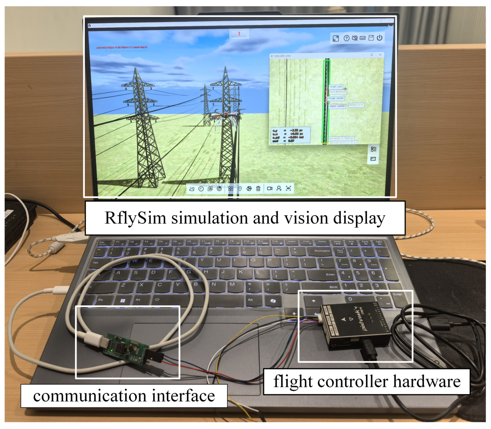
Experiments were conducted on the RflySim–PX4 hardware-in-the-loop platform shown in Figure 4, using a fixed overhead-ground-wire scene. The experiments evaluate visual tracking, robustness to perturbations, and the contribution of historical-input weighting. Local-model comparisons, parameter sensitivity, and computation time are also examined.

4.1. Experimental Platform and Evaluation Metrics

The platform consists of flight-control hardware, the RflySim simulation environment, and the visual-control program [32]. The flight-control inner loop runs on the hardware, while RflySim supplies the UAV dynamics, sensor feedback, three-dimensional scene, and onboard-camera images. The visual-control program converts YOLO11s-OBB detections into velocity and yaw-rate commands. Each visual-error component was processed by an independent constant-velocity Kalman filter before being used for control. 

Table 1. Common HIL platform, visual-perception, and experimental settings.

Item	Value	Item	Value
Inertia matrix $\mathit{J}$	$0.0211,0.0219,0.0366\mathrm{kg}{\mathrm{m}}^2$	Mass m	$1.4$ kg
Arm length	$0.225$ m	Motor time constant ${\tau }_m$	$0.05$ s
Camera offset	$[0.1,0,0]$ m	Camera FOV	${90}^{\circ }$
Image resolution	$640\times 480$	Reference width $w_{\mathrm{ref}}$	35 px
Visual rate	20 Hz	Control rate	100 Hz
Run duration	40 s	Inference mean/p95	$11.39/28.89$ ms
Scales $(s_x,s_w,s_{\psi })$	$(80,20,0.5)$	Command bounds	$(0.20,0.30,0.60)$
Detector	YOLO11s-OBB	Selected OBB	Highest confidence
Object class	Wire (one class)	Dataset source	RflySim
Training images	800	Validation images	200
Input size	640	Batch size	16
Training epochs	100	Detector training seed	0
Confidence	$0.25$	NMS IoU	$0.70$
Precision	$1.000$	Recall	$0.994$
${\mathrm{mAP}}_{50}$	$0.995$	${\mathrm{mAP}}_{50:95}$	$0.779$

The command bounds are symmetric; the entries for $(v_y,v_z,r)$ are given in $\mathrm{m}/\mathrm{s}$, $\mathrm{m}/\mathrm{s}$, and $\mathrm{rad}/\mathrm{s}$, respectively.

lists the platform and visual-detection settings, and

Table 2. Default parameters of the proposed MHW-PAJ-CLF controller.

Parameter	Value	Parameter	Value
$\mathrm{diag}\left({\mathit{B}}_0\right)$	$(-5.55,1.00,-2.30)$	$\beta$	$0.80$
${\theta }_{\min }$	$(-11.25,1.00,-8.00)$	${\theta }_{\max }$	$(-0.50,12.50,-0.30)$
$N_d$	10	$\gamma$	$0.02$
$\lambda$	$0.04$	$u_{\mathrm{th}}$	$0.03$
$(ϵ,{ϵ}_r,{ϵ}_u)$	$({10}^{-2},{10}^{-6},{10}^{-4})$	$({\rho }_a,{\rho }_{\delta })$	$(0.01,100)$
$\kappa$	$0.60$	$\mathrm{diag}\left(\mathit{W}\right)$	$(1,2,8)$

gives the MHW-PAJ-CLF parameters.

The controller parameters were adjusted progressively according to the closed-loop responses, considering success rate, transient overshoot, and oscillations in the tracking errors and control commands. Table 2 gives the resulting parameter values. The parameter settings of the baseline methods are listed in

Table 3. Parameter settings of the baseline methods.

Method	Parameter Group	Setting
PID	Channel gains	$K_p=(0.002,0.010,0.40)$; $K_i=(0.00005,0.0002,0)$; $K_d=(0,0,0.005)$.
ADRC	x channel	${({\omega }_c,{\omega }_o,b_0)}_x=(0.13,1.4,360)$.
	w channel	${({\omega }_c,{\omega }_o,b_0)}_w=(0.5,2.5,100)$.
	$\psi$ channel	${({\omega }_c,{\omega }_o,b_0)}_{\psi }=(1.5,5.0,6.0)$.
NVPC	Prediction/visibility	$N_p=16$; $\Delta t=0.05$ s; ${\rho }_v=220$; minimum normalized edge margin $=0.18$.
	Cost weights	$Q=(0.45,0.80,0.40)$; $R=(0.70,0.25,0.60)$; $R_{\Delta }=(6.00,1.50,2.00)$.
	Command damping	Smoothing coefficient $=0.88$; damping blend $=0.95$; proportional gain $=0.25$; error-rate gains $=(1.20,0.20,0.15)$.
RBF-IBVS	Basis functions	27 centers on ${\{-1,0,1\}}^3$; Gaussian width $=0.85$.
	Adaptive update	Learning rate $=0.025$; leakage $=0.02$; compensation gain $=0.55$.
	Control parameters	Convergence rate $=0.48$; ${\widehat{f}}_{\max }=(1.20,1.00,0.45)$.

.

PID and ADRC use independent three-channel feedback structures, with ADRC additionally using extended-state observation. NVPC balances predicted tracking error, command magnitude, and command changes, with a visibility penalty that discourages motion toward the image boundary. RBF-IBVS uses Gaussian basis functions to estimate and compensate for local model error. The baseline parameters were adjusted progressively according to the observed closed-loop responses. The selected baseline parameters were kept fixed across the five evaluation runs. PID uses bounded integral accumulation and command clipping; ADRC commands are clipped to their prescribed bounds; NVPC projects candidate inputs into the admissible range; and the RBF-IBVS output is limited before command application. These controller-generated commands are subject to the common bounds listed in Table 1. All five methods use the same detector and visual-filter settings, initial conditions, sampling rates, bounds on the controller-generated commands, and success criterion. Results presented as the mean ± sample standard deviation are calculated from five runs. The numerical results in the tables are rounded to the precision shown, and the reported percentage changes in tracking error are calculated from the displayed mean values. The best mean values are shown in bold in the comparison tables.

For the initial-pose, noise-and-dropout, and command-bias conditions in Section 4.3, PAJ-CLF and MHW-PAJ-CLF were each evaluated in five runs using run seeds $12,001$–$12,005$. The same seed was assigned to the two methods for each repetition.

The mean absolute error measures tracking accuracy in each visual channel. The overall tracking error $E_q$ combines the three normalized errors:

$$E_q=\sqrt{{\displaystyle \frac{1}{N}}\sum _{k=1}^N{\parallel {\mathit{q}}_k\parallel }_2^2},$$

(56)

where N is the number of observations. A smaller $E_q$ indicates a smaller overall tracking error.

For each run, the success rate is the percentage of the total run duration during which all three visual errors simultaneously satisfy the following tolerances:

$$|e_x| \le 8\mathrm{px},|e_w| \le 3\mathrm{px},|e_{\psi }| \le 0.10\mathrm{rad}.$$

For results reported as a mean, the success rates are averaged over five runs.

The local-response residual $E_B$ is computed consistently across the local-model update methods, using the preceding control model and the most recent historical input for prediction:

$$E_B=\sqrt{{\displaystyle \frac{1}{3N_h}}\sum _{k\in \mathcal{H}}{\parallel {\dot{\mathit{q}}}_k-{\mathit{B}}_{c,k-1}{\mathit{u}}_{k-1}\parallel }_2^2},$$

(57)

where $\mathcal{H}$ contains the consecutive valid visual observations used to calculate the response errors throughout the run and $N_h=\left|\mathcal{H}\right|$. A smaller $E_B$ indicates closer agreement between the model prediction and the observed visual response.

4.2. Visual-Tracking Performance

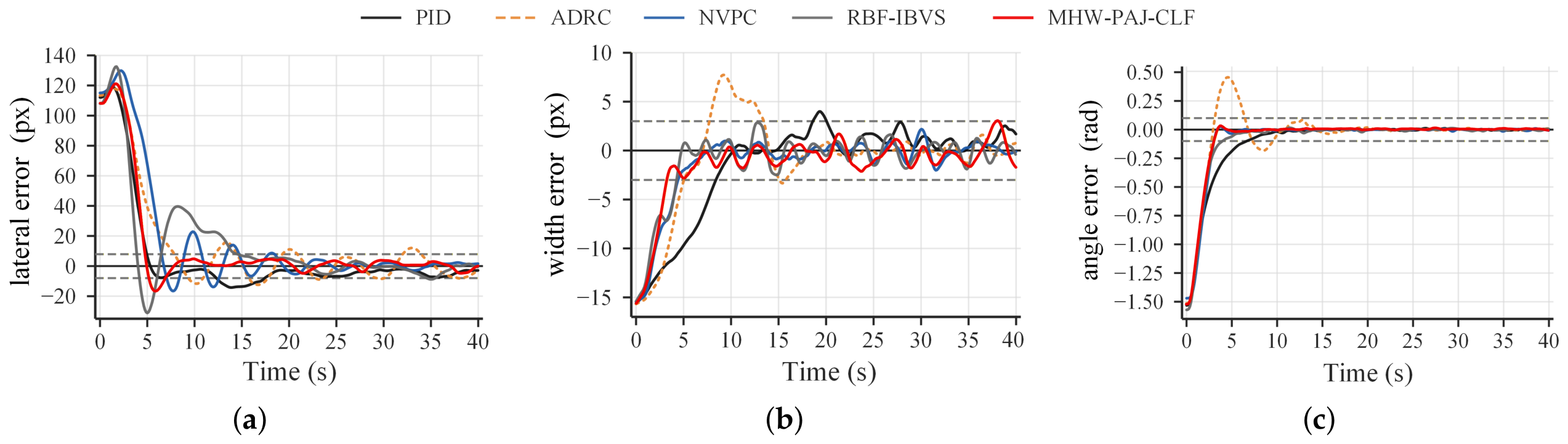
The visual-tracking comparison included MHW-PAJ-CLF, PID, ADRC, an NVPC baseline adapted from [33], and RBF-IBVS [20]. Figure 5 shows the lateral-position, apparent-width, and angle-error responses. 

Table 4. Visual-tracking performance of the five methods.

Method	$\overline{|{\mathit{e}}_{\mathit{x}}|}$ (px)	$\overline{|{\mathit{e}}_{\mathit{w}}|}$ (px)	$\overline{|{\mathit{e}}_{\mathit{\psi }}|}$ (rad)	Success Rate (%)
PID	$15.592\pm 0.843$	$3.526\pm 0.137$	$0.09993\pm 0.00168$	$37.82\pm 11.43$
ADRC	$25.038\pm 0.700$	$2.891\pm 0.083$	$0.11644\pm 0.00103$	$46.44\pm 3.59$
NVPC	$36.380\pm 0.492$	$2.983\pm 0.041$	$0.18845\pm 0.00070$	$40.91\pm 2.40$
RBF-IBVS	$20.878\pm 3.323$	$2.188\pm 0.058$	$0.09308\pm 0.00026$	$64.45\pm 7.14$
MHW-PAJ-CLF	$\mathbf{15}.\mathbf{201}\pm 3.564$	$\mathbf{2}.\mathbf{005}\pm 0.222$	$\mathbf{0}.\mathbf{07561}\pm 0.00446$	$\mathbf{75}.\mathbf{50}\pm 6.10$

Bold values indicate the best mean performance in each column.

compares the tracking errors and success rates.

MHW-PAJ-CLF achieves the lowest mean absolute error in all three visual channels. Its lateral-position error is 2.51% lower than that of PID, the best baseline for this channel. The improvements in apparent width and angle are larger: relative to RBF-IBVS, the best baseline for these two channels, the errors decrease by 8.36% and 18.77%, respectively.

MHW-PAJ-CLF achieves a mean success rate of 75.50%, exceeding the 64.45% of RBF-IBVS by 11.05 percentage points. Together with the reductions in width and angle errors, the higher success rate shows that the proposed controller improves coordinated regulation of the three visual variables while maintaining lateral alignment accuracy.

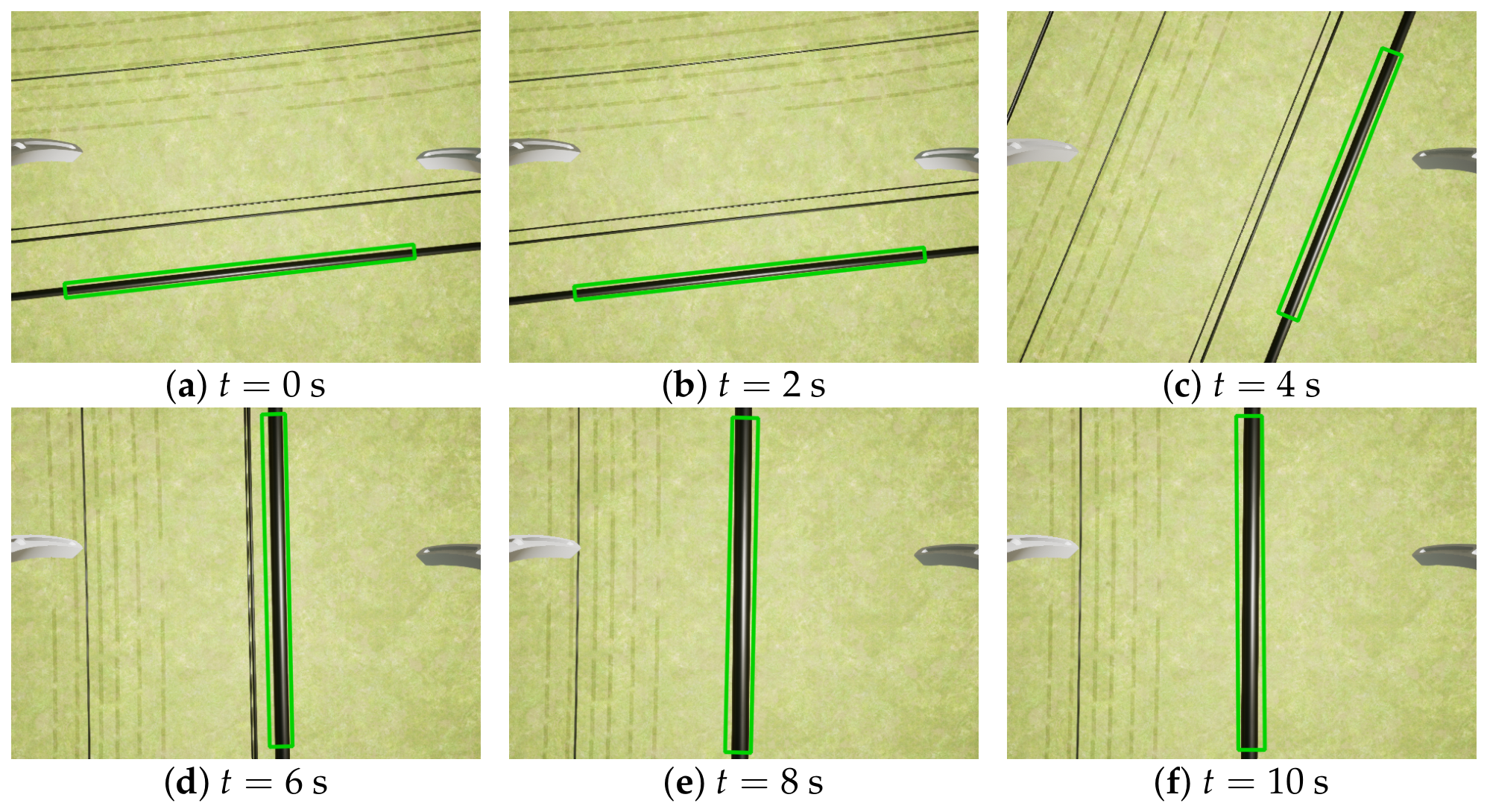
Figure 6 shows the YOLO11s-OBB detections during the initial closed-loop phase.

4.3. Performance Under Perturbations and Temporal Lag

To assess tracking robustness, PAJ-CLF and MHW-PAJ-CLF are compared under changes in initial pose, measurement noise and frame dropout, command bias, and additional visual-feedback delay.

Table 5. Tracking and local-response prediction under different perturbations.

Test	Tracking RMSE ${\mathit{E}}_{\mathit{q}}$		Local-Response Residual ${\mathit{E}}_{\mathit{B}}$
	PAJ	MHW	PAJ	MHW
Reference	$0.780\pm 0.119$	$\mathbf{0}.\mathbf{716}\pm \mathbf{0}.\mathbf{037}$	$0.270\pm 0.101$	$\mathbf{0}.\mathbf{237}\pm \mathbf{0}.\mathbf{057}$
Initial pose	$0.803\pm 0.222$	$\mathbf{0}.\mathbf{714}\pm \mathbf{0}.\mathbf{051}$	$0.256\pm 0.054$	$\mathbf{0}.\mathbf{250}\pm \mathbf{0}.\mathbf{014}$
Noise + dropout	$0.745\pm 0.039$	$\mathbf{0}.\mathbf{707}\pm \mathbf{0}.\mathbf{022}$	$0.432\pm 0.014$	$\mathbf{0}.\mathbf{413}\pm \mathbf{0}.\mathbf{015}$
Command bias	$0.799\pm 0.038$	$\mathbf{0}.\mathbf{761}\pm \mathbf{0}.\mathbf{039}$	$0.278\pm 0.020$	$\mathbf{0}.\mathbf{264}\pm \mathbf{0}.\mathbf{019}$
Delay, 100 ms	$0.735\pm 0.006$	$\mathbf{0}.\mathbf{728}\pm \mathbf{0}.\mathbf{016}$	$0.234\pm 0.014$	$\mathbf{0}.\mathbf{226}\pm \mathbf{0}.\mathbf{007}$
Delay, 200 ms	$0.758\pm 0.018$	$\mathbf{0}.\mathbf{737}\pm \mathbf{0}.\mathbf{005}$	$0.248\pm 0.019$	$\mathbf{0}.\mathbf{242}\pm \mathbf{0}.\mathbf{006}$

Bold values indicate the lower mean value for each metric under each test condition.

summarizes the results.

The initial-pose condition introduces a lateral displacement of $0.70$ m, a height change of $1.0$ m, and a yaw offset of ${10}^{°}$ relative to the reference condition. The noise-and-dropout condition uses measurement-noise standard deviations of 4 px, $1.5$ px, and $0.02$ rad for the lateral-position, apparent-width, and orientation-angle errors, respectively, with a $0.5$ s frame dropout beginning at 12 s.

The command-bias condition applies offsets of $0.08$ m/s, $0.06$ m/s, and $0.06$ rad/s to the lateral-velocity, vertical-velocity, and yaw-rate commands, respectively, during 10–25 s, with 1 s linear onset and removal ramps. These offsets are added after controller output limiting. Additional visual-feedback delays of 100 and 200 ms are evaluated separately.

MHW-PAJ-CLF achieves lower mean tracking error $E_q$ and local-response prediction error $E_B$ in every condition in Table 5. The largest reduction in tracking error, 11.08%, occurs under initial-pose variation, where the standard deviation also decreases from 0.222 to 0.051. This combination indicates more accurate and more consistent tracking as the initial pose changes. Under noise and frame dropout and under command bias, the mean tracking error decreases by 5.10% and 4.76%, respectively.

With additional visual-feedback delays of 100 and 200 ms, MHW-PAJ-CLF retains lower mean tracking errors than PAJ-CLF. Its $E_q$ values are 0.728 and 0.737, compared with 0.735 and 0.758 for PAJ-CLF, respectively.

The relationship between the control-method output ${\mathit{u}}_c$ and the command applied through the flight-control interface, ${\mathit{u}}_a$, is represented by the first-order dynamics

$${\tau }_a{\dot{\mathit{u}}}_a+{\mathit{u}}_a={\mathit{u}}_c,$$

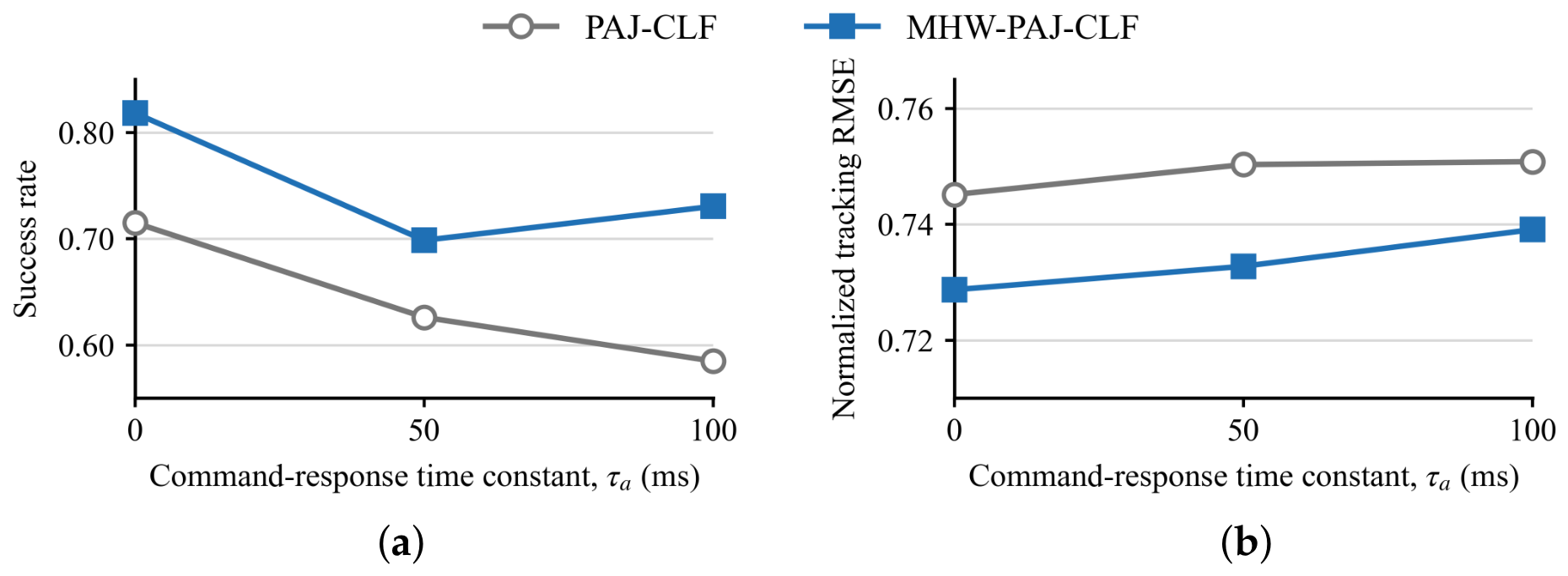
where ${\tau }_a$ is the time constant of the first-order element imposed at the command interface; when ${\tau }_a=0$, this element satisfies ${\mathit{u}}_a={\mathit{u}}_c$. Figure 7 and

Table 6. Visual-tracking metrics at different command-response time constants.

${\mathit{\tau }}_{\mathit{a}}$ (ms)	Method	$\overline{|{\mathit{e}}_{\mathit{x}}|}$ (px)	$\overline{|{\mathit{e}}_{\mathit{w}}|}$ (px)	$\overline{|{\mathit{e}}_{\mathit{\psi }}|}$ (rad)	Success Rate (%)	${\mathit{E}}_{\mathit{q}}$
0	PAJ-CLF	16.608	1.912	0.08249	71.51	0.7451
0	MHW-PAJ-CLF	14.440	1.806	0.07126	81.83	0.7287
50	PAJ-CLF	16.963	2.164	0.08362	62.61	0.7503
50	MHW-PAJ-CLF	16.204	1.829	0.07359	69.86	0.7328
100	PAJ-CLF	17.414	2.099	0.08350	58.49	0.7508
100	MHW-PAJ-CLF	16.040	1.840	0.07670	73.06	0.7391

compare the tracking performance at ${\tau }_a=0$, 50 ms, and 100 ms.

MHW-PAJ-CLF achieves smaller mean absolute errors in all three channels at each command-response time constant. As ${\tau }_a$ increases from 0 to 100 ms, its $E_q$ rises from 0.7287 to 0.7391 and remains below that of PAJ-CLF. At 100 ms, the success rate is 73.06%, compared with 58.49% for PAJ-CLF. Together with the visual-feedback-delay results, these findings show that multi-history updating retains its tracking benefit under both delayed visual feedback and slower command response.

Across the 60 PAJ-CLF and MHW-PAJ-CLF runs, the Pearson and Spearman correlations between $E_B$ and $E_q$ are $0.282$ and $0.420$, respectively. These modest positive correlations indicate that lower prediction errors tend to accompany lower tracking errors. In closed-loop operation, the estimated response gains also shape the feedback commands, so tracking performance depends on both prediction accuracy and the resulting control action.

4.4. Analysis of Historical-Input Weighting

Table 7. Control performance of the local-model update methods.

Method	${\mathit{E}}_{\mathit{q}}$	${\mathit{E}}_{\mathit{B}}$	${\mathit{T}}_{\mathbf{first}}$ (s)	${\mathit{T}}_{3\mathbf{s}}$ (s)
Fixed-${\mathit{B}}_0$-CLF	$0.7500\pm 0.0345$	$0.2379\pm 0.0229$	$9.13\pm 1.79$	$10.44\pm 2.60$
PAJ-CLF	$0.7798\pm 0.1187$	$0.2703\pm 0.1005$	$7.63\pm 2.06$	$10.00\pm 5.55$
MHW-PAJ-CLF	$0.7162\pm 0.0368$	$0.2372\pm 0.0572$	$5.91\pm 1.68$	$10.13\pm 3.14$

compares the fixed nominal model, single-history PAJ update, and multi-history-weighted PAJ update within the same CLF-QP control framework. The time $T_{\mathrm{first}}$ measures when all three errors first satisfy their tolerances, and $T_{3\mathrm{s}}$ marks the start of the first interval in which they remain within the tolerances for at least 3 s.

MHW-PAJ-CLF achieves the lowest mean tracking error and reaches the three error tolerances $3.22$ s earlier than the fixed model and $1.72$ s earlier than PAJ-CLF, on average. The mean $T_{3\mathrm{s}}$ values are close, ranging from $10.00$ to $10.44$ s. MHW-PAJ-CLF and the fixed model also have similar mean $E_B$ values. The main improvements therefore concern the initial reduction of the visual errors and overall closed-loop tracking.

During the first 10 s, the mean $E_q$ values are $1.493\pm 0.067$, $1.550\pm 0.232$, and $1.425\pm 0.073$ for the fixed model, PAJ-CLF, and MHW-PAJ-CLF, respectively. The corresponding mean lateral feedback gains are $0.108$, $0.121$, and $0.168$, and the mean RMS lateral-velocity commands are $0.110$, $0.124$, and $0.134$ m/s. As described in Section 3.4, the estimated response gain determines the feedback gain used to generate the command. The larger initial feedback gain of MHW-PAJ-CLF produces stronger lateral corrections, which are consistent with its earlier first entry and lower initial tracking error.

Table 8. Ablation of historical-input weighting.

Weighting	${\mathit{E}}_{\mathit{q}}$	$\mathbf{\Delta }{\mathit{E}}_{\mathit{q}}$ (%)
Full	0.7162$\pm$0.0368	–
Uniform	0.7287 ± 0.0297	+1.75
Error only	0.7268 ± 0.0293	+1.48
Shared	0.7298 ± 0.0330	+1.90

Bold entries indicate the method with the lowest mean tracking error.

examines the weighting rule through three alternatives. Uniform weighting assigns equal weights to all historical inputs; response-error-only weighting uses their prediction errors; shared weighting applies the same weights to all three visual channels.

The full configuration determines the weights separately for each channel using both prediction error and input magnitude. It achieves the lowest mean $E_q$ among the tested configurations. Uniform weighting, response-error-only weighting, and shared weighting give mean errors that are 1.75%, 1.48%, and 1.90% higher, respectively. These results support the combined weighting rule used by MHW-PAJ.

The weighted mean history position describes whether the weights favor more recent or earlier inputs:

$${\overline{d}}_{i,k}={\displaystyle \sum _{j=0}^{J_k}}j{w}_{i,k}^{\left(j\right)},$$

(58)

The equivalent number of historical inputs measures how widely the weights are distributed:

$$N_{\mathrm{eff},i,k}={\left[{\displaystyle \sum _{j=0}^{J_k}}{\left(w_{i,k}^{\left(j\right)}\right)}^2\right]}^{-1}.$$

(59)

A larger ${\overline{d}}_{i,k}$ indicates greater weighting toward earlier inputs, while a larger $N_{\mathrm{eff},i,k}$ indicates that more historical inputs share the weights.

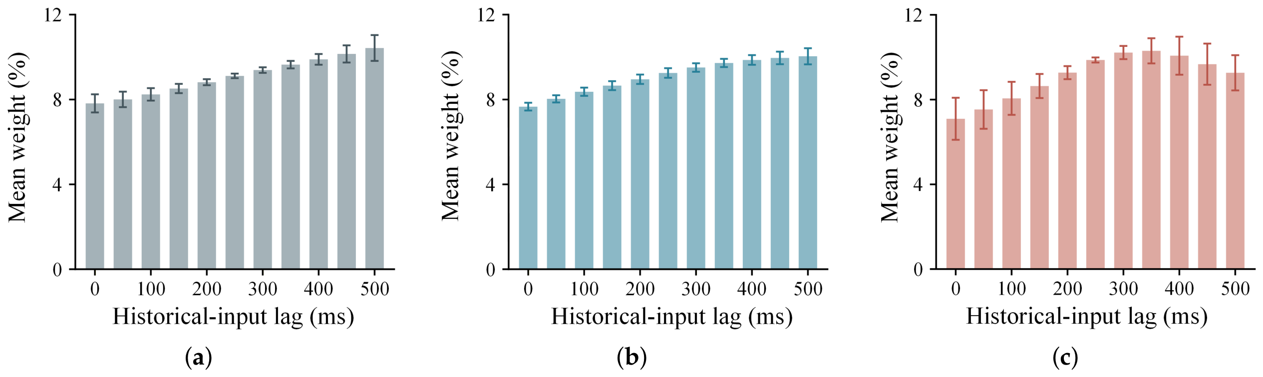
Figure 8 shows the historical-input weights in the lateral-position, apparent-width, and angle channels. Each bar corresponds to one history position, ordered from the newest input on the left to the oldest on the right. With a nominal visual-update interval of 50 ms, 0 ms denotes the most recent input and 500 ms denotes the input ten updates earlier.

The mean weights range from approximately $7.1\%$ to $10.4\%$, showing that multiple historical inputs contribute to the update. The lateral-position and apparent-width channels give slightly higher weights to older inputs, while the angle channel gives higher weights to inputs at 300–400 ms. Each channel uses prediction error and input magnitude to weight the parameter corrections associated with these historical inputs, then combines the corrections to update its local response gain.

Table 9. Historical-input weight statistics.

Channel	Mean ${\overline{\mathit{d}}}_{\mathit{i}}$ (Steps)	Mean ${\mathit{N}}_{\mathbf{eff},\mathit{i}}$
Lateral	$5.294\pm 0.106$	$10.258\pm 0.258$
Width	$5.268\pm 0.058$	$9.346\pm 0.173$
Angle	$5.297\pm 0.245$	$9.526\pm 0.364$

gives mean equivalent numbers of historical inputs between $9.35$ and $10.26$ within the eleven-input window, further indicating that the update draws on a broad part of the available history.

With additional visual-feedback delays of 0, 100, and 200 ms, the weighted mean history positions in the three channels, expressed in time units, are $(265,263,265)$, $(270,263,278)$, and $(263,262,282)$ ms, respectively. Increasing the additional delay from 0 to 200 ms changes these mean positions by $-1.7$, $-1.6$, and $17.1$ ms. The weighted mean history position characterizes the center of the gain-update weight distribution over the input history. Its value depends on the input amplitudes, prediction errors, and available history length.

4.5. Comparison of Diagonal and Full Local Image-Response Models

The controller uses ${\mathit{B}}_0$ as a preset nominal matrix, while ${\widehat{\mathit{B}}}_{\mathrm{diag}}$ and ${\widehat{\mathit{B}}}_{\mathrm{full}}$ are diagonal and full local constant models identified from experimental data. Both models use the input–response relation

$${\dot{\mathit{q}}}_k\approx \mathit{B}{\mathit{u}}_{k-1}.$$

(60)

Pseudo-random binary inputs are used to obtain the identification data at the reference viewpoint and within the command limits listed in Table 1. The full and diagonal models are identified by multivariable and channel-wise least squares, respectively, and evaluated using validation data. The rows correspond to $q_x$, $q_w$, and $q_{\psi }$, and the columns correspond to $v_y$, $v_z$, and r. The identified matrices are

$${\widehat{\mathit{B}}}_{\mathrm{full}}=\left[\begin{array}{ccc}-0.6550& 0.0534& -0.0981\\ 0.0391& 0.5213& -0.0249\\ 0.0402& 0.0269& -1.0741\end{array}\right],{\widehat{\mathit{B}}}_{\mathrm{diag}}=\mathrm{diag}(-0.6720,0.5332,-1.0763).$$

(61)

The corresponding diagonal elements of ${\widehat{\mathit{B}}}_{\mathrm{full}}$ and ${\widehat{\mathit{B}}}_{\mathrm{diag}}$ differ by 2.52%, 2.23%, and 0.20%.The ratio between the Frobenius norms of the off-diagonal and diagonal parts of ${\widehat{\mathit{B}}}_{\mathrm{full}}$ is 9.57%. The largest off-diagonal element is $B_{13}=-0.0981$, whose magnitude is 14.98% of the main diagonal element in the same row. The validation RMSE values of the two models are summarized in

Table 10. Validation RMSE values of the diagonal and full local image-response models.

Model	${\mathit{q}}_{\mathit{x}}$	${\mathit{q}}_{\mathit{w}}$	${\mathit{q}}_{\mathit{\psi }}$	Overall
Diagonal	0.1805	0.2877	0.1525	0.2150
Full	0.1837	0.2883	0.1525	0.2161

.

For predictions of the normalized visual-state rate, the overall validation RMSE values of the diagonal and full models are 0.2150 and 0.2161, respectively. At the reference viewpoint and within the tested command range, the three corresponding input–output channels provide the dominant responses, supporting the use of a diagonal local image-response structure for control.

4.6. Parameter Sensitivity and Computation Time

Table 11. Effect of the slack-penalty coefficient ${\rho }_{\delta }$ on control performance.

${\mathit{\rho }}_{\mathit{\delta }}$	${\mathit{E}}_{\mathit{q}}$	Mean Slack
50	$0.7188\pm 0.0232$	0.0360
100	$0.7162\pm 0.0368$	0.0340
200	$\mathbf{0}.\mathbf{7150}\pm \mathbf{0}.\mathbf{0207}$	0.0350

Bold values indicate the lowest mean value in each performance column.

examines how the CLF-QP slack penalty ${\rho }_{\delta }$ affects tracking performance at values of 50, 100, and 200.

Across this range, the mean $E_q$ varies by 0.53%, and the mean slack remains between 0.0340 and 0.0360. The small change in mean error indicates stable tracking performance over this parameter range, which includes the reference value ${\rho }_{\delta }=100$.

The adaptive gain $\gamma$ sets the strength of the response-error correction, while the history depth $N_d$ sets the extent of the input history used for updating.

Table 12. Effects of adaptive gain and history depth on control performance.

$\mathit{\gamma }$	${\mathit{N}}_{\mathit{d}}$	${\mathit{E}}_{\mathit{q}}$
$0.01$	10	$0.768\pm 0.071$
$0.02$	10	$0.716\pm 0.037$
$0.04$	10	$\mathbf{0}.\mathbf{711}\pm \mathbf{0}.\mathbf{030}$
$0.02$	5	$0.721\pm 0.020$
$0.02$	15	$0.752\pm 0.030$

Bold values indicate the lowest mean tracking error among the tested parameter settings.

examines their effects on tracking performance.

With $N_d=10$, increasing $\gamma$ from 0.01 to 0.02 reduces the mean $E_q$ from 0.768 to 0.716. A further increase to 0.04 gives a smaller reduction to 0.711. Thus, strengthening the correction has a larger benefit at the lower gains, and the reference value of 0.02 achieves mean tracking performance close to that at 0.04.

With $\gamma =0.02$, history depths of 5 and 10 give similar mean $E_q$ values of 0.721 and 0.716, while a depth of 15 gives a higher value of 0.752. A longer window incorporates more distant commands into the local-response update. The lower errors at depths 5 and 10 support the reference history depth of 10 under the tested conditions.

The controller computation times are summarized in

Table 13. Controller computation time under the repeated reference setting.

Method	Mean (ms)	p95 (ms)
PAJ-CLF	0.037	0.107
MHW-PAJ-CLF	0.038	0.113

. The mean computation times of PAJ-CLF and MHW-PAJ-CLF are 0.037 and 0.038 ms, respectively, and their 95th-percentile times are 0.107 and 0.113 ms. For MHW-PAJ-CLF, the 95th-percentile time occupies 1.13% of the 10 ms control period, supporting the dual-rate configuration with channel-gain updates at 20 Hz and CLF-QP command generation at 100 Hz.

5. Discussion

The five-method comparison highlights the contribution of MHW-PAJ-CLF to coordinated visual regulation. It maintains lateral alignment accuracy while improving apparent-width and angle regulation, increasing the proportion of time during which all three visual errors simultaneously satisfy their tolerances.

MHW-PAJ-CLF and the fixed model have similar mean prediction errors, and MHW-PAJ-CLF reaches all three error tolerances earlier. Online updates of the local model adjust the feedback gains through the nominal control law and influence the commands generated by the CLF-QP. During the first 10 s, MHW-PAJ-CLF exhibits a larger lateral feedback gain and lateral-velocity command magnitude, consistent with its lower initial tracking error and earlier simultaneous satisfaction of all three error tolerances.

MHW-PAJ combines parameter corrections associated with several preceding inputs. Each visual channel weights these corrections according to prediction error and input magnitude. The full weighting rule gives the lowest mean tracking error among the tested configurations, and the comparisons with PAJ-CLF show that its tracking benefit extends to additional visual-feedback delay and command-response lag.

The three-channel local model is used near the reference pose, and closed-loop performance is evaluated through HIL experiments in a fixed overhead-ground-wire scene. The experiments did not include controlled variations in illumination or scene background, so robustness to these changes remains unverified. Future work will evaluate the effects of illumination and background variation on visual tracking, alongside adaptive history-window selection and real-flight validation.

6. Conclusions

This paper develops MHW-PAJ-CLF for three-channel close-range UAV visual servoing near overhead ground wires. The method uses response error and input magnitude to assign weights to historical inputs separately for each channel. It then takes the weighted sum of the corresponding PAJ parameter corrections. The update includes a correction toward the nominal value, and projection restricts the estimated response parameter of each channel to its prescribed interval. The updated estimate and the nominal model are combined in a prescribed proportion. The CLF-QP uses this model to regulate the three visual errors within the input limits.

Across five HIL runs, MHW-PAJ-CLF achieves mean absolute lateral-position, apparent-width, and angle errors of $15.201$ px, $2.005$ px, and $0.07561$ rad, respectively, and a mean success rate of $75.50\%$. Compared with the best baseline for each visual-error metric, the three mean absolute errors decrease by $2.51\%$, $8.36\%$, and $18.77\%$, respectively. The mean success rate exceeds that of RBF-IBVS by $11.05$ percentage points. In the reference comparison with PAJ-CLF, the mean time to first satisfy all three error tolerances decreases from $7.63$ to $5.91$ s. Under initial-pose variation, measurement noise and frame dropout, control-command bias, additional visual-feedback delay, and different command-response time constants, MHW-PAJ-CLF achieves a lower overall tracking error $E_q$ than PAJ-CLF. The three simplified weighting configurations have mean tracking errors 1.48–1.90% above that of the full configuration, and the 95th-percentile computation time of MHW-PAJ-CLF is 0.113 ms. These HIL results support the use of multi-history weighting to improve close-range UAV visual tracking under visual-feedback delay and command-response lag.

References

1. Ahmed, F.; Mohanta, J.C.; Keshari, A. Power transmission line inspections: Methods, challenges, current status and usage of unmanned aerial systems. J. Intell. Robot. Syst. 2024, 110, 54. [Google Scholar] [CrossRef] [Scilit]
2. Diniz, L.F.; Pinto, M.F.; Melo, A.G.; Honorio, L.M. Visual-based assistive method for UAV power line inspection and landing. J. Intell. Robot. Syst. 2022, 106, 41. [Google Scholar] [CrossRef] [Scilit]
3. Guan, H.; Sun, X.; Su, Y.; Hu, T.; Wang, H.; Wang, H.; Peng, C.; Guo, Q. UAV-LiDAR aids automatic intelligent powerline inspection. Int. J. Electr. Power Energy Syst. 2021, 130, 106987. [Google Scholar] [CrossRef] [Scilit]
4. Xing, J.; Cioffi, G.; Hidalgo-Carrio, J.; Scaramuzza, D. Autonomous power line inspection with drones via perception-aware MPC. In Proceedings of the 2023 IEEE/RSJ International Conference on Intelligent Robots and Systems (IROS), Detroit, MI, USA, 1–5 October 2023; pp. 1086–1093. [Google Scholar] [CrossRef] [Scilit]
5. Ollero, A.; Suarez, A.; Papaioannidis, C.; Pitas, I.; Marredo, J.M.; Hoang, V.D.; Ebeid, E.; Kratky, V.; Saska, M.; Hanoune, C.; et al. Multi-aerial robotic system for power line inspection and maintenance: Comparative analysis from the AERIAL-CORE final experiments. IEEE Trans. Field Robot. 2025, 2, 549–573. [Google Scholar] [CrossRef] [Scilit]
6. Zhang, H.; Wu, L.; Chen, Y.; Chen, R.; Kong, S.; Wang, Y.; Hu, J.; Wu, J. Attention-guided multitask convolutional neural network for power line parts detection. IEEE Trans. Instrum. Meas. 2022, 71, 5008213. [Google Scholar] [CrossRef] [Scilit]
7. Liu, Z.; Wu, G.; He, W.; Fan, F.; Ye, X. Key target and defect detection of high-voltage power transmission lines with deep learning. Int. J. Electr. Power Energy Syst. 2022, 142, 108277. [Google Scholar] [CrossRef] [Scilit]
8. Choudhary, S.; Saurav, S.; Gidde, P.; Saini, R.; Singh, S. LPC-Det: Attention-based lightweight object detector for power line component detection in UAV images. Comput. Electr. Eng. 2025, 126, 110476. [Google Scholar] [CrossRef] [Scilit]
9. Xu, Y.; Xu, Z.; Wang, H.; Wei, Z.; Wu, Z. Instance-level orientation enhancement for horizontal box supervised oriented object detection in remote sensing images. IEEE Trans. Image Process. 2025, 34, 7613–7626. [Google Scholar] [CrossRef] [Scilit] [PubMed]
10. Lin, Y.X.; Lai, Y.C. Deep Learning-Based Navigation System for Automatic Landing Approach of Fixed-Wing UAVs in GNSS-Denied Environments. Aerospace 2025, 12, 324. [Google Scholar] [CrossRef] [Scilit]
11. Wang, G.; Qin, J.; Liu, Q.; Ma, Q.; Zhang, C. Image-based visual servoing of quadrotors to arbitrary flight targets. IEEE Robot. Autom. Lett. 2023, 8, 2022–2029. [Google Scholar] [CrossRef] [Scilit]
12. Li, Y.; Lu, G.; He, D.; Zhang, F. Robocentric model-based visual servoing for quadrotor flights. IEEE/ASME Trans. Mechatron. 2023, 28, 2155–2166. [Google Scholar] [CrossRef] [Scilit]
13. Xie, H.; Fink, G.; Lynch, A.F.; Jagersand, M. Adaptive visual servoing of UAVs using a virtual camera. IEEE Trans. Aerosp. Electron. Syst. 2016, 52, 2529–2538. [Google Scholar] [CrossRef] [Scilit]
14. Lin, J.; Wang, Y.; Miao, Z.; Fan, S.; Wang, H. Robust observer-based visual servo control for quadrotors tracking unknown moving targets. IEEE/ASME Trans. Mechatron. 2023, 28, 1268–1279. [Google Scholar] [CrossRef] [Scilit]
15. Lin, J.; Wang, Y.; Miao, Z.; Wang, H.; Fierro, R. Robust image-based landing control of a quadrotor on an unpredictable moving vehicle using circle features. IEEE Trans. Autom. Sci. Eng. 2023, 20, 1429–1440. [Google Scholar] [CrossRef] [Scilit]
16. Kumar, Y.; Shamsi, B.P.; Roy, S.B.; Sujit, P.B. Tracking a planar target using image-based visual servoing technique. IEEE Trans. Intell. Veh. 2024, 9, 4362–4372. [Google Scholar] [CrossRef] [Scilit]
17. Yang, K.; Bai, C.; She, Z.; Quan, Q. High-speed interception multicopter control by image-based visual servoing. IEEE Trans. Control Syst. Technol. 2025, 33, 119–135. [Google Scholar] [CrossRef] [Scilit]
18. Yang, J.; Liu, X.; Sun, J.; Li, S. Sampled-data robust visual servoing control for moving target tracking of an inertially stabilized platform with a measurement delay. Automatica 2022, 137, 110105. [Google Scholar] [CrossRef] [Scilit]
19. Chen, Y.; Li, B.; Shi, W.; Zhang, X. Image-based visual servoing of micro aerial vehicles with robust observation and output feedback. IEEE Trans. Control Syst. Technol. 2025, 33, 1995–2004. [Google Scholar] [CrossRef] [Scilit]
20. Sepahvand, S.; Janabi-Sharifi, F.; Masnavi, H.; Aghili, F.; Amiri, N. Robust image-based visual servoing of an aerial robot using self-organizing neural networks. Int. J. Control Autom. Syst. 2024, 22, 3762–3776. [Google Scholar] [CrossRef] [Scilit]
21. Yang, Q.; Li, H. RMPC-based visual servoing for trajectory tracking of quadrotor UAVs with visibility constraints. IEEE/CAA J. Autom. Sin. 2024, 11, 2027–2029. [Google Scholar] [CrossRef] [Scilit]
22. Zhou, Y.; Xu, F.; Zhou, Y.; Zhang, Z.; Wang, H. Constrained image-based visual servoing with a sampling-based planning framework. IEEE/ASME Trans. Mechatron. 2025, 30, 4899–4909. [Google Scholar] [CrossRef] [Scilit]
23. Liu, Q.; Mao, J.; Han, L.; Zhang, C.; Yang, J. Predictive observer-based dual-rate prescribed performance control for visual servoing of robot manipulators with view constraints. IEEE Trans. Cybern. 2025, 55, 2424–2436. [Google Scholar] [CrossRef] [Scilit] [PubMed]
24. Yi, X.; Luo, B.; Zhao, Y. Neural network-based robust guaranteed cost control for image-based visual servoing of quadrotor. IEEE Trans. Neural Netw. Learn. Syst. 2024, 35, 12693–12705. [Google Scholar] [CrossRef] [Scilit] [PubMed]
25. Byun, W.; Huh, S.; Jang, H.; Yu, S.; Lim, S.; Lee, S.; Nam, W. Vector Field-Based Robust Quadrotor Landing on a Moving Ground Platform. Aerospace 2025, 12, 590. [Google Scholar] [CrossRef] [Scilit]
26. Zhang, L.; Lin, Y.; Chen, Y.; Wang, A.; Ren, Z. Data-driven generalized iterative predictive control with IESO for UAV trajectory tracking. Int. J. Control Autom. Syst. 2026, 24, 1156–1170. [Google Scholar] [CrossRef] [Scilit]
27. Guo, H.; Song, T.; Ye, J.; Abdulrahman, Y.; Gu, X.; Jiang, T.; Dong, Y. Image-Based Visual Servoing for Quadrotor Formation Encirclement and Tracking of Unknown Targets. Aerospace 2026, 13, 138. [Google Scholar] [CrossRef] [Scilit]
28. Pan, Y.; Shi, T. Adaptive estimation and control with online data memory: A historical perspective. IEEE Control Syst. Lett. 2024, 8, 267–278. [Google Scholar] [CrossRef] [Scilit]
29. Li, Z.; Lai, B.; Pan, Y. Image-based composite learning robot visual servoing with an uncalibrated eye-to-hand camera. IEEE/ASME Trans. Mechatron. 2024, 29, 2499–2509. [Google Scholar] [CrossRef] [Scilit]
30. Kamath, A.K.; Feroskhan, M. Augmented dynamics visual servoing: Mapping image variations to multirotor’s input commands. IEEE Trans. Aerosp. Electron. Syst. 2025, 61, 14928–14942. [Google Scholar] [CrossRef] [Scilit]
31. Kamath, A.K.; Yan, B.; Shi, P.; Feroskhan, M. Physics-informed Koopman neural operator for augmented dynamics visual servoing of multirotors. IEEE Trans. Autom. Sci. Eng. 2026, 23, 4639–4653. [Google Scholar] [CrossRef] [Scilit]
32. Wang, S.; Dai, X.; Ke, C.; Quan, Q. RflySim: A rapid multicopter development platform for education and research based on Pixhawk and MATLAB. In Proceedings of the 2021 International Conference on Unmanned Aircraft Systems (ICUAS), Athens, Greece, 15–18 June 2021; pp. 1587–1594. [Google Scholar] [CrossRef] [Scilit]
33. Zhang, Y.; Yao, J.; Qian, C. Event-triggered nonlinear visual predictive control strategy for robots. J. Intell. Robot. Syst. 2025, 111, 80. [Google Scholar] [CrossRef] [Scilit]
Figure 1. Physical task geometry and visual-error definition: (a) physical geometry and reference-command directions; (b) image-space visual errors.
Aerospace 13 00844 g001
Figure 2. Height–width calibration from five viewpoints.
Aerospace 13 00844 g002
Figure 3. Closed-loop structure and signal flow of the proposed MHW-PAJ-CLF control method. Arrows indicate the direction of signal flow; the superscript asterisk denotes the optimal control command obtained by solving the CLF-QP.
Aerospace 13 00844 g003
Figure 4. RflySim–PX4 HIL platform and visual-control program.
Aerospace 13 00844 g004
Figure 5. Visual-error responses of the five methods: (a) lateral-position error; (b) apparent-width error; (c) angle error. The gray dashed lines indicate the error tolerance limits: ± 8 px in (a), ± 3 px in (b), and ± 0.10 rad in (c).
Aerospace 13 00844 g005
Figure 6. YOLO11s-OBB detection results during the initial closed-loop phase: (af) successive visual observations from 0 to 10 s. The green boxes indicate the oriented bounding boxes of the overhead ground wire detected by YOLO11s-OBB.
Aerospace 13 00844 g006
Figure 7. Visual-tracking performance at different command-response time constants: (a) success rate; (b) normalized tracking root-mean-square error E q .
Aerospace 13 00844 g007
Figure 8. Historical-input weights in the (a) lateral-position, (b) apparent-width, and (c) angle channels. Bar heights and error bars show the mean and sample standard deviation of the run-averaged weights across five reference runs.
Aerospace 13 00844 g008