Perspective-n-Point Post Optimization for Far-Field Pose Measurement Based on Weighted Central Normalization

Abstract

Far-field vision-based pose measurement is a crucial technology for applications such as high-resolution Earth observation and space security early warning. However, owing to the perspective imaging model of long-range optical systems, conventional vision-based pose measurement methods are highly susceptible to image noise and pose parameter coupling, leading to significant estimation deviations. Consequently, these methods fail to meet the rigorous requirements for the accurate measurement and intelligent perception of object poses in far-field scenarios, particularly when the object distance significantly exceeds the focal length. To address these challenges, this paper presents a Perspective-n-Point (PnP) preprocessing and post-optimization method for far-field pose measurement based on weighted central normalization. First, the Robust PnP (RPnP) algorithm is employed to obtain an initial pose for the far-field object, and an objective function is formulated by minimizing the reprojection error of the image feature points. Second, central normalization is applied to the Jacobian matrix of the pose parameters, and the information matrix is weighted according to the localization uncertainty of the image feature points. Finally, a weighted nonlinear optimization is executed to obtain refined pose parameters. Under the tested conditions, this approach can reduce the sensitivity of the pose parameters to image noise, minimizes the coupling among extrinsic parameters, and reduces the tendency of noise-driven pose-update excursions. The proposed method is evaluated through simulations and scaled physical relative-comparison experiments, supporting its potential for numerically stable vision-based pose measurement of far-field objects in aerospace and related domains. Noise-and-turbulence simulations demonstrate the pose-refinement benefit of CS and improved rotation estimation with a known spatial covariance model.

1. Introduction

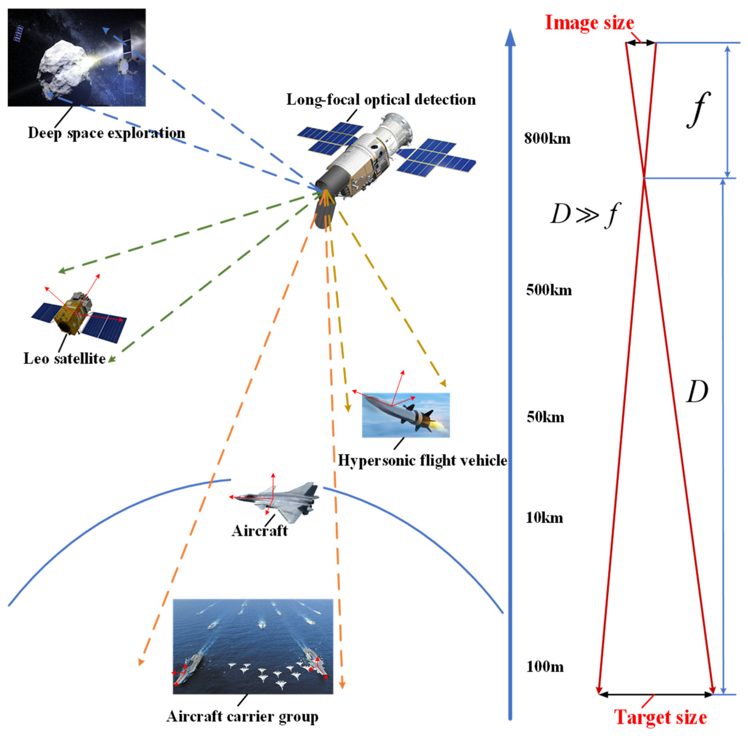
Far-field vision-based pose measurement is an enabling technique for high-resolution Earth observation, space-target monitoring, and long-range optical surveillance. Recent Remote Sensing studies have addressed aircraft pose estimation from keypoints and structural constraints, non-cooperative space-target pose estimation through cross-source point-cloud fusion, and monocular pose determination for robotic capture operations [1,2,3]. Broader reviews summarize electro-optical pose-determination architectures and the practical limitations of monocular navigation for cooperative and uncooperative spacecraft [4,5]. Model-based pose refinement has also been demonstrated in autonomous rendezvous and docking and in aerial-video georegistration [6,7]. Representative scenarios include deep-space observation, on-orbit monitoring, and ground-based tracking with telephoto optical systems. In these settings, object distances may range from 10⁴ to 10⁶ m, whereas the focal length is typically 1–10 m, so the distance-to-focal-length ratio can reach 10³–10⁵. By comparison, near-field measurements usually involve distances of 0.5–10 m and focal lengths of approximately 8–50 mm. Consequently, depth variations across a far-field object contribute only weakly to the overall range, and the imaging geometry approaches a parallel-projection regime. For on-orbit servicing, debris inspection, and spacecraft rendezvous, the estimated optical pose supplies state information to guidance and attitude-control subsystems, while compact nanosatellite attitude actuators provide a complementary downstream example [8]. Representative far-field measurement scenarios are illustrated in Figure 1.

Under far-field conditions, the small perspective variation across the target makes the estimated pose highly sensitive to image-localization perturbations. The Jacobian columns associated with rotation and translation can also differ by several orders of magnitude and exhibit strong correlation, so a small reprojection residual may coexist with substantial drift along depth or coupled pose directions. Robust geometric initialization and numerically balanced local refinement are therefore both required.

The Perspective-n-Point (PnP) problem and its numerical properties have been studied extensively [9]. Linear projective methods such as DLT [10] are inexpensive, but the projective design matrix loses effective numerical rank as the imaging geometry approaches the affine limit, increasing the noise sensitivity of depth-related coefficients. Minimal and closed-form solvers, including P3P variants [11,12], EPnP [13], DLS [14], UPnP [15], and SQPnP [16], improve algebraic efficiency and solution selection; their far-field accuracy remains governed by the weak perspective information in the observations. Iterative and robust formulations such as POSIT [17], globally convergent pose estimation [18], RPnP [19], planar-target methods [20], and algebraic outlier rejection [21] improve initialization, redundancy, or mismatch resistance, while the subsequent local system still inherits the rotation-translation scale imbalance. RPnP is therefore selected as the initializer and followed by conditioning-oriented refinement.

Learning-based methods improve the image evidence supplied to geometric pose estimation. EPro-PnP [22], differentiable RANSAC-based localization [23], PVNet [24], and the Spacecraft Pose Network [25] estimate keypoints, correspondences, or pose distributions in difficult imagery. Maximum-likelihood PnP [26], covariance-aware point-and-line estimation [27], and probabilistic relocalization [28] further improve the statistical treatment of localization uncertainty. These approaches address measurement reliability, whereas Jacobian preconditioning addresses scale imbalance and near-null pose directions.

Nonlinear refinement is commonly implemented through bundle adjustment, Gauss–Newton, or Levenberg–Marquardt (LM) iterations [29,30,31,32] with calibrated camera intrinsics and a consistent perspective model [33,34]. In far-field geometry, a single damping scale acts on rotational and translational coordinates whose Jacobian columns may differ by several orders of magnitude, allowing high-sensitivity directions to dominate the update. The present method therefore inserts a numerical preprocessing stage between RPnP initialization and LM refinement: each Jacobian column is centered in residual space, scaled by its current norm, and optionally combined with feature-localization weights. Centering and scaling follow established principles of numerical preconditioning, and covariance weighting follows weighted least squares; their integration here is tailored to the far-field PnP update.

The main contributions are as follows:

• A far-field PnP refinement pipeline is formulated that separates RPnP initialization, conditioning-oriented Jacobian preprocessing, optional uncertainty weighting, and step acceptance using the original reprojection objective.
• Residual-space centering and per-iteration column scaling balance the Jacobian columns and reduce sensitivity to common-mode residual perturbations. Their effects on the information matrix and weak pose directions are analyzed explicitly.
• Feature-localization uncertainty is incorporated through a weighted information matrix. Simulations evaluate localization noise, atmospheric turbulence, target distance, feature count, initialization, and individual optimization components. Scaled physical experiments assess the resulting relative-pose measurement performance.

The remainder of this paper is organized as follows. Section 2 presents the imaging model, RPnP initialization, central normalization, and uncertainty-weighted optimization. Section 3 reports simulation and physical experiments. Section 4 discusses the findings and limitations, and Section 5 concludes the paper.

2. Materials and Methods

2.1. Method Overview

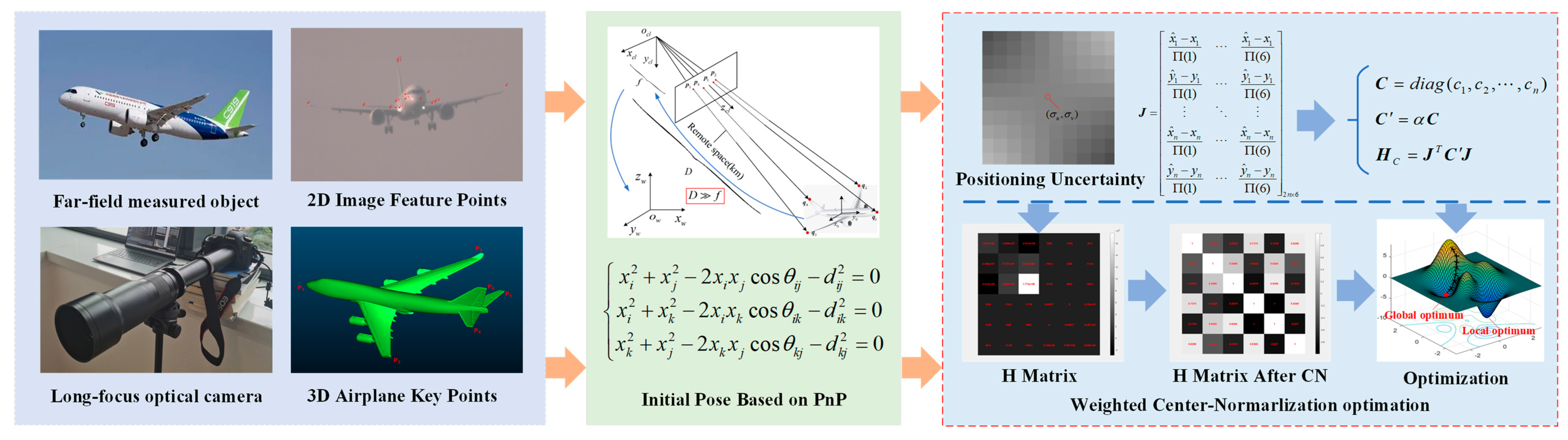
The proposed workflow is shown in Figure 2. The 2D image feature points and their corresponding 3D object points are first acquired. RPnP then estimates the initial pose. An objective function is constructed from the reprojection residuals, the Jacobian matrix is centrally normalized, and each residual is weighted according to the localization uncertainty of the corresponding feature point. The normalized weighted LM iteration produces the refined far-field pose.

2.2. Perspective Projection and Initial Pose Estimation

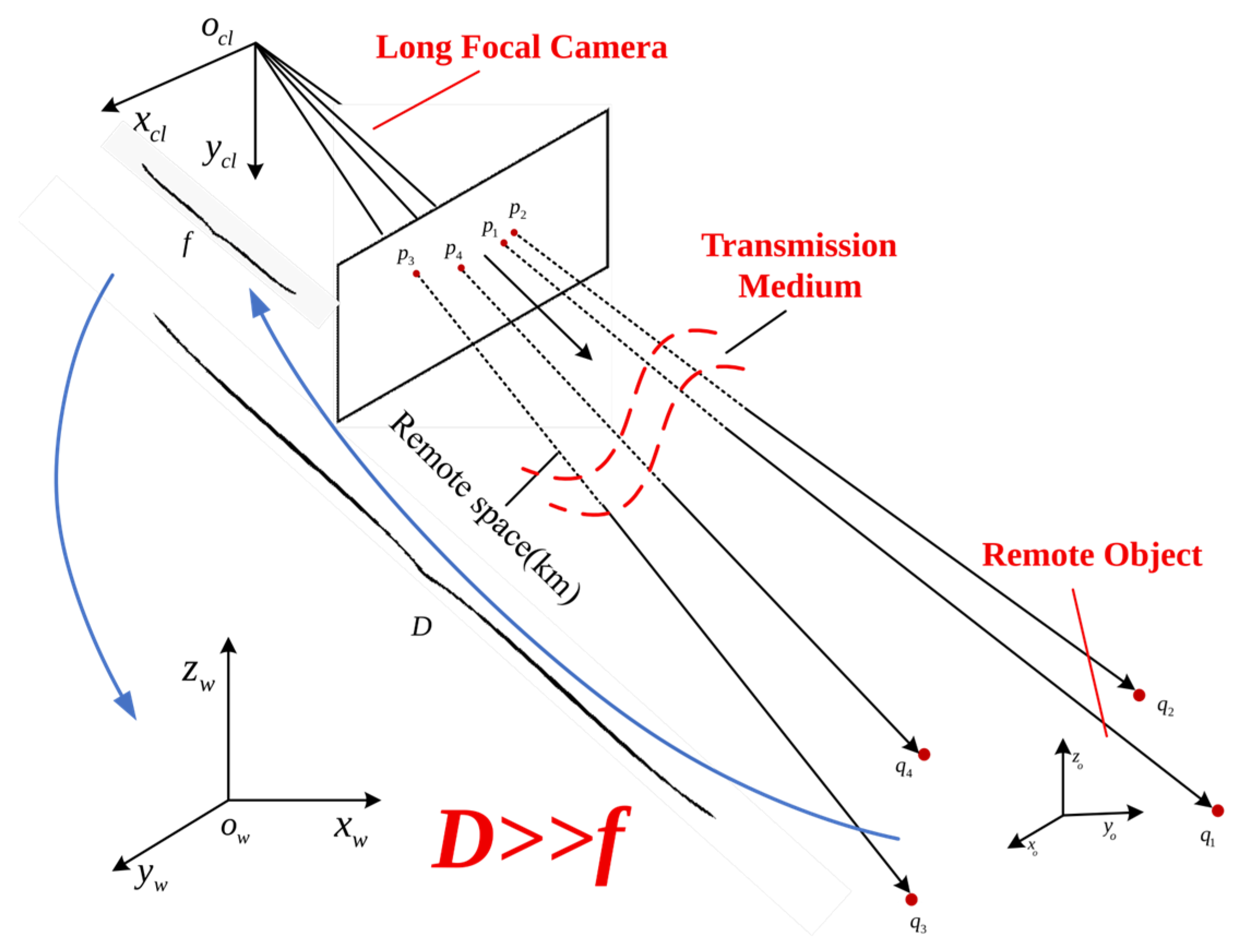
Let the known object points be ${\mathbf{P}}_i=[X_i,Y_i,Z_i{]}^{\mathrm{T}}$ and their image observations be ${\mathbf{p}}_i=[x_i,y_i{]}^{\mathrm{T}}$, for $i=1,\dots ,n$. The pinhole projection relationship is illustrated in Figure 3 and written as

$$s_i\left[\begin{array}{c}{x}_i\\ y_i\\ 1\end{array}\right]=\mathbf{K}\left[\begin{array}{cc}\mathbf{R}& \mathbf{t}\end{array}\right]\left[\begin{array}{c}{X}_i\\ Y_i\\ Z_i\\ 1\end{array}\right], \mathbf{K}=\left[\begin{array}{ccc}{f}_x& \gamma & u_0\\ 0& f_y& v_0\\ 0& 0& 1\end{array}\right]$$

(1)

where s_i ≠ 0 is the projective scale, $f_x$ and $f_y$ are the focal lengths in pixels, (u₀,v₀) is the principal point, and γ is the skew coefficient. The rotation matrix R and translation vector t define the object pose with respect to the camera. Lens distortion is corrected before pose estimation using calibrated radial and tangential coefficients [33,34].

RPnP is used to determine the initial pose [19]. The two object points with the largest image separation define a stable reference baseline, and the remaining points form multiple three-point subsets. For each subset, the law of cosines gives

$$\left\{\begin{array}{l}{x}^2+y^2-2xy\mathrm{c}\mathrm{o}\mathrm{s}{\theta }_1-d_1^2=0,\\ y^2+z^2-2yz\mathrm{c}\mathrm{o}\mathrm{s}{\theta }_2-d_2^2=0,\\ z^2+x^2-2zx\mathrm{c}\mathrm{o}\mathrm{s}{\theta }_3-d_3^2=0,\end{array}\right.$$

(2)

where x, y, and z are the depths of the three points, d₁, d₂, d₃ are their known pairwise Euclidean distances, and θ₁, θ₂, θ₃ are the angles between the corresponding camera rays.

Algebraic elimination converts each three-point subset into a univariate quartic polynomial,

$$g_i\left(x\right)=a_i{x}^4+b_i{x}^3+c_i{x}^2+d_{i}x+e_i,$$

(3)

and the full set of subset constraints is collected as

$$\mathbf{g}\left(x\right)={\left[\begin{array}{cccc}{g}_1\left(x\right)& g_2\left(x\right)& \cdots & g_{n-2}\left(x\right)\end{array}\right]}^T.$$

(4)

The squared polynomial residuals form the scalar cost

$$G\left(x\right)={\displaystyle \sum _{i=1}^{n-2}}{g}_i^2\left(x\right),$$

(5)

whose stationary points satisfy

$$G^{\prime }\left(x\right)=2{\displaystyle \sum _{i=1}^{n-2}}{g}_i\left(x\right){g_i}^{\prime }\left(x\right)=0.$$

(6)

The physically valid roots are evaluated using the reprojection error. After reconstructing the point depths, a rotation axis is established from a pair of 3D points, and the rotation is represented as

$$\mathbf{R}={\mathbf{R}}_0\mathrm{R}\mathrm{o}\mathrm{t}\left({\mathbf{z}}_c,\theta \right).$$

(7)

A homogeneous linear system is then solved by singular-value decomposition to recover the rotation angle and translation vector. The resulting RPnP pose is used only as the initial estimate for the proposed post-optimization.

2.3. Analysis of the Information Matrix

For a least-squares pose problem, the approximate information matrix is the Gauss–Newton Hessian. Its diagonal elements reflect the local sensitivity of the residuals to each parameter, whereas its off-diagonal elements reflect parameter correlations. Large differences between diagonal terms and large off-diagonal terms indicate unbalanced observability and strong coupling. A large Jacobian condition number further amplifies measurement noise in the estimated update.

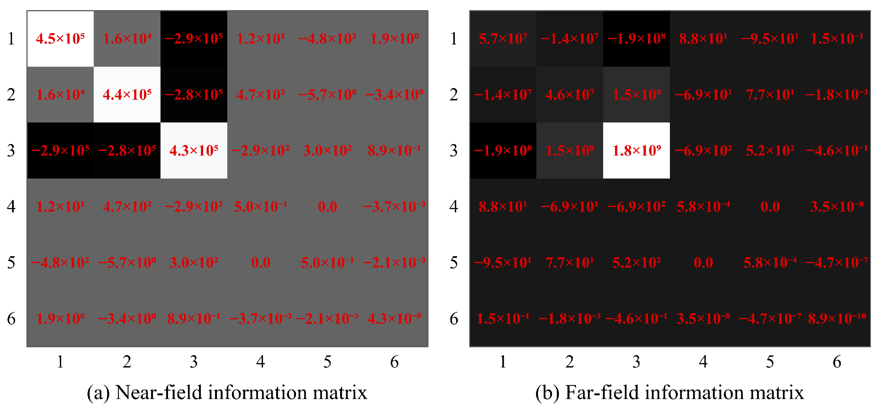
Figure 4 compares the information matrices obtained in a near-field simulation at an object distance of 0.1 km and a far-field simulation at 1000 km. In the near field, the absolute diagonal values range from approximately 4.3 × 10⁻⁵ to 4.5 × 10⁵, while in the far field they range from approximately 8.9 × 10⁻¹⁰ to 1.8 × 10⁹. The far-field matrix therefore exhibits a substantially greater scale imbalance and stronger off-diagonal coupling.

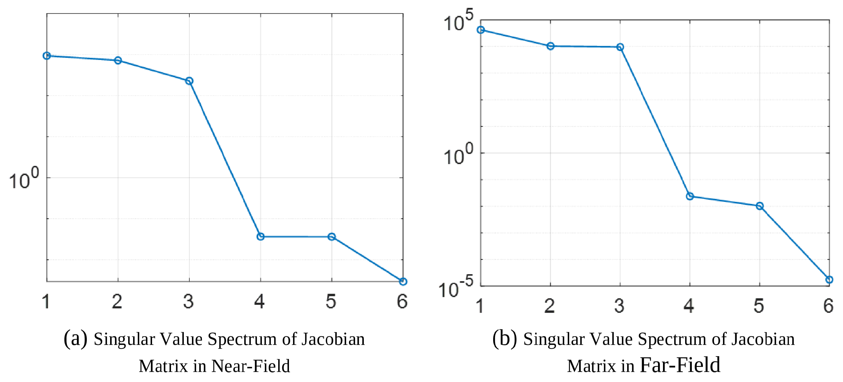
The corresponding singular-value spectra are shown in Figure 5. The Jacobian condition number increases from approximately 5.13 × 10⁵ in the near field to 2.61 × 10⁹ in the far field, and the singular values span a much wider range. This behavior explains why a conventional unscaled nonlinear iteration becomes sensitive to small feature perturbations at long range.

2.4. Central Normalization of the Jacobian Matrix

Let Π denote the six-dimensional pose-parameter vector. The reprojection-error objective is

$$\underset{\mathsf{\Pi }}{\mathrm{m}\mathrm{i}\mathrm{n}}F\left(\mathsf{\Pi }\right)={\displaystyle \sum _{i=1}^n}\left[{\left({\widehat{x}}_i-x_i\right)}^2+{\left({\widehat{y}}_i-y_i\right)}^2\right],$$

(8)

where $({\widehat{x}}_i,{\widehat{y}}_i)$ is the projection of $P_i$ under the current pose and

$$\mathsf{\Pi }={\left[\begin{array}{cccccc}{r}_x& r_y& r_z& t_x& t_y& t_z\end{array}\right]}^T.$$

(9)

Using the residual vector r(Π), the first-order approximation at iteration k is

$$\mathbf{r}\left({\mathsf{\Pi }}_k+{\mathbf{d}}_k\right)\approx \mathbf{r}\left({\mathsf{\Pi }}_k\right)+{\mathbf{J}}_k{\mathbf{d}}_k,$$

(10)

with the Jacobian

$${\mathbf{J}}_k={\left.{\displaystyle \frac{\partial \mathbf{r}\left(\mathsf{\Pi }\right)}{\partial \mathsf{\Pi }}}\right|}_{{\mathsf{\Pi }}_k}\in {\mathbb{R}}^{2n\times 6}.$$

(11)

The Gauss–Newton information matrix is

$${\mathbf{H}}_k={\mathbf{J}}_k^T{\mathbf{J}}_k,$$

(12)

and the LM update is

$${\mathbf{d}}_k=-{\left({\mathbf{H}}_k+\lambda \mathbf{I}\right)}^{-1}{\mathbf{J}}_k^T\mathbf{r}\left({\mathsf{\Pi }}_k\right),$$

(13)

Here, $\lambda >0$ is the damping parameter. The damping is reduced after a successful step and increased when the objective does not decrease, balancing the update size and numerical stability [30,31,32].

To reduce the far-field scale imbalance, the columns of the Jacobian are first centered. Let 1_2n denote a vector of ones and let $\overline{j}$ contain the column means. The centered Jacobian is

$${\mathbf{J}}_c=\mathbf{J}-1_{2n}{\bar{\mathbf{J}}}^T,$$

(14)

where the mean of column q is

$${\bar{J}}_q={\displaystyle \frac{1}{2n}}{\displaystyle \sum _{i=1}^{2n}}{J}_{iq}.$$

(15)

Each centered column is then normalized by its Euclidean norm,

$${J^{\prime }}_{iq}={\displaystyle \frac{J_{iq}-{\bar{J}}_q}{s_q}},$$

(16)

with

$$s_q={\left[{\displaystyle \sum _{i=1}^{2n}}{\left(J_{iq}-{\bar{J}}_q\right)}^2\right]}^{1/2}.$$

(17)

The centrally normalized information matrix becomes

$${\mathbf{H}}^{\prime }={{\mathbf{J}}^{\prime }}^T{\mathbf{J}}^{\prime }.$$

(18)

Equations (14)–(18) can be written in matrix form. Define the residual-space centering matrix as

$$\mathbf{C}={\mathbf{I}}_{2n}-{\displaystyle \frac{1}{2n}}{\mathbf{1}}_{2n}{\mathbf{1}}_{2n}^{\mathrm{T}}.$$

(19)

For Jacobian columns ${\mathbf{j}}_q$, the diagonal scale and normalized Jacobian are

$$\mathbf{D}=\mathrm{d}\mathrm{i}\mathrm{a}\mathrm{g}\left(\Vert \mathbf{C}{\mathbf{j}}_1{\Vert }_2,\dots ,\Vert \mathbf{C}{\mathbf{j}}_6{\Vert }_2\right), {\mathbf{J}}^{\prime }=\mathbf{C}\mathbf{J}{\mathbf{D}}^{-1}.$$

(20)

The centering matrix satisfies

$${\mathbf{C}}^{\mathrm{T}}=\mathbf{C}, {\mathbf{C}}^2=\mathbf{C}, \mathbf{C}{1}_{2n}=0.$$

(21)

Substitution into the normalized information matrix gives

$${\mathbf{H}}^{\prime }={\mathbf{D}}^{-1}\left[{\mathbf{J}}^{\mathrm{T}}\mathbf{J}-{\displaystyle \frac{1}{2n}}\left({\mathbf{J}}^{\mathrm{T}}{\mathbf{1}}_{2n}\right){\left({\mathbf{J}}^{\mathrm{T}}{\mathbf{1}}_{2n}\right)}^{\mathrm{T}}\right]{\mathbf{D}}^{-1}.$$

(22)

Centering subtracts the common-mode contribution from the Jacobian Gram matrix. For nonzero centered columns, $\mathbf{D}$ is nonsingular and normalizes their Euclidean norms, balancing the local rotational and translational sensitivities.

The normalized LM step is transformed back using the diagonal scale, as specified in Equations (30) and (31). The candidate pose is evaluated by the weighted reprojection objective

$$\Phi \left(\mathsf{\Pi }\right)=\mathbf{r}\left(\mathsf{\Pi }{)}^{\mathrm{T}}\mathbf{W}\mathbf{r}\right(\mathsf{\Pi }),$$

(23)

where $\mathbf{W}={\mathbf{I}}_{2n}$ for unweighted CS. A candidate step ${\mathbf{d}}_k$ is accepted when

$$\Phi ({\mathsf{\Pi }}_k+{\mathbf{d}}_k)<\Phi \left({\mathsf{\Pi }}_k\right).$$

(24)

The pose is expressed in local Rodrigues coordinates. Scaling is reversed in the pose update, while centering acts on the residual-space linearization. The increment relation $d_{k,q}^{*}=s_q{d}_{k,q}$ gives $d_k=D^{-1}{d}_k^{*}$. The star and prime both denote the normalized increment in Equations (29)–(31). Inverse scaling restores parameter units; objective consistency additionally requires retaining the residual-space mean contribution.

The effect on weak directions follows from

$$\mathbf{J}\mathbf{v}=\mathbf{0} ⟹ \mathbf{C}\mathbf{J}\mathbf{v}=\mathbf{0}, \mathrm{r}\mathrm{a}\mathrm{n}\mathrm{k}\left(\mathbf{C}\mathbf{J}\right)\le \mathrm{r}\mathrm{a}\mathrm{n}\mathrm{k}\left(\mathbf{J}\right).$$

(25)

Every null direction of the original Jacobian remains a null direction after centering. The operation balances the working system and can introduce further null directions; physical depth observability remains determined by the camera–target geometry.

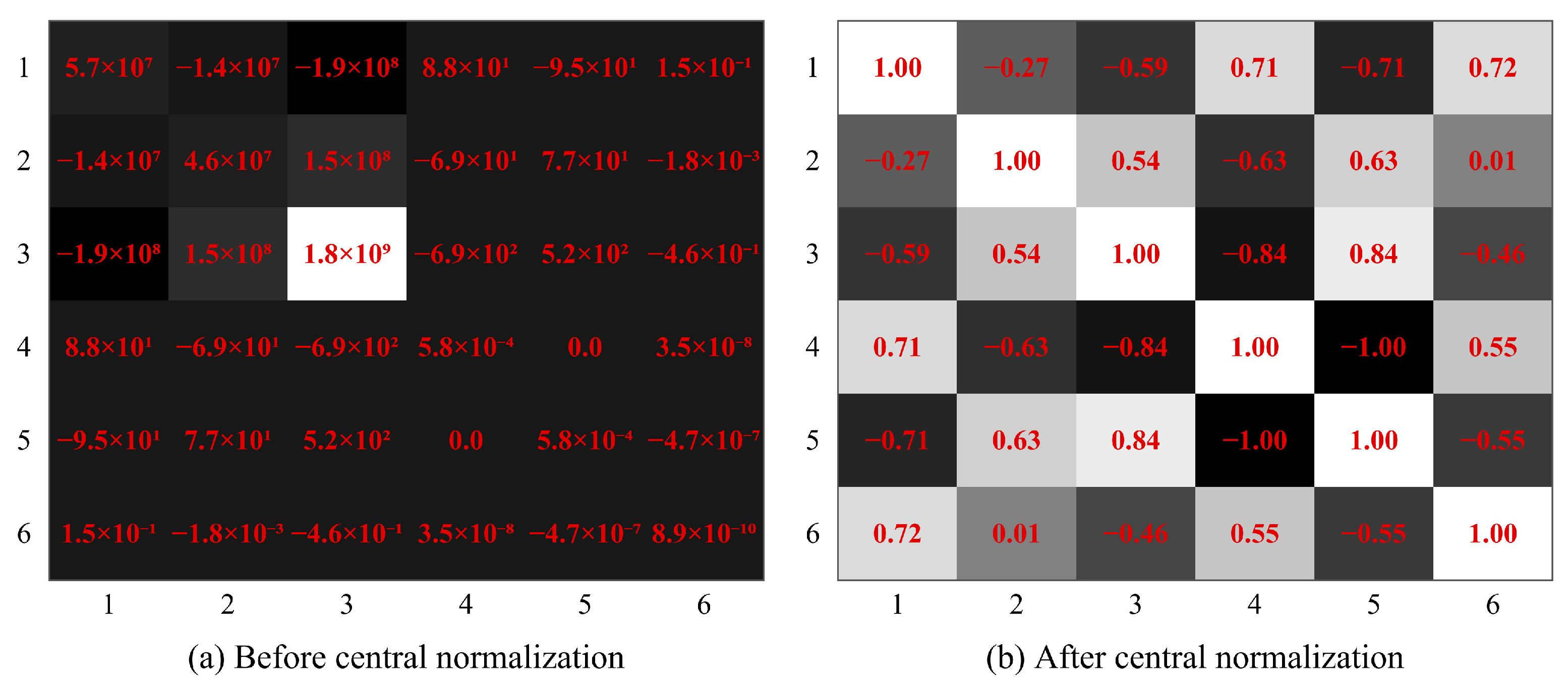
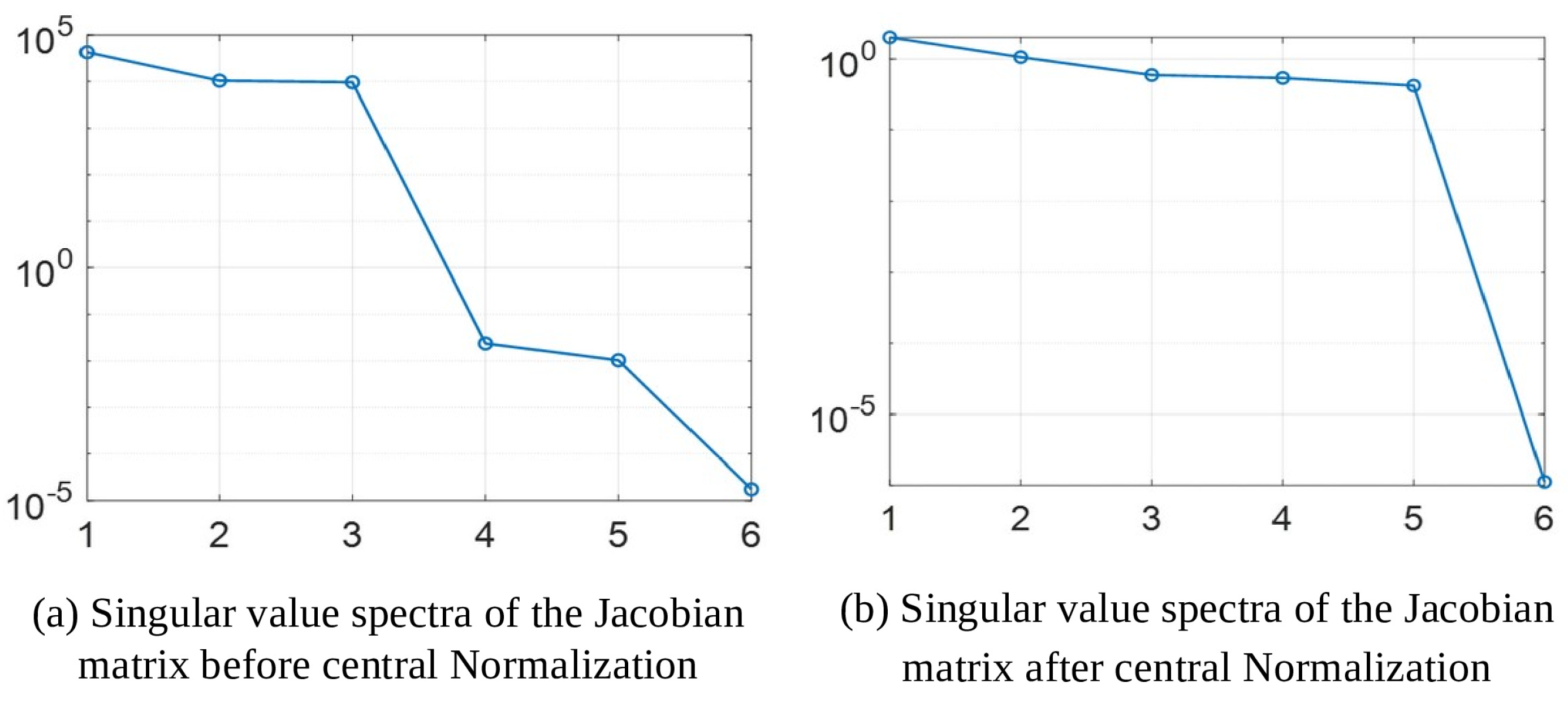
Because each normalized column has unit Euclidean norm, the diagonal terms of H′ are unity, and the off-diagonal terms directly represent normalized column correlations. Figure 6 shows that the large magnitude disparities in the original information matrix are removed. Figure 7 shows that the Jacobian condition number decreases from 2.61 × 10⁹ to 2.24 × 10⁶ and that the singular-value spectrum becomes substantially more compact.

2.5. Uncertainty-Weighted Optimization

Central normalization alone assigns equal importance to all image residuals. In practice, feature points can have different localization accuracies because of blur, low contrast, occlusion, or perspective deformation. For feature point i, the inverse-variance weight matrix is defined as

$${\mathbf{W}}_i=\left[\begin{array}{cc}{\sigma }_{x,i}^{-2}& 0\\ 0& {\sigma }_{y,i}^{-2}\end{array}\right],$$

(26)

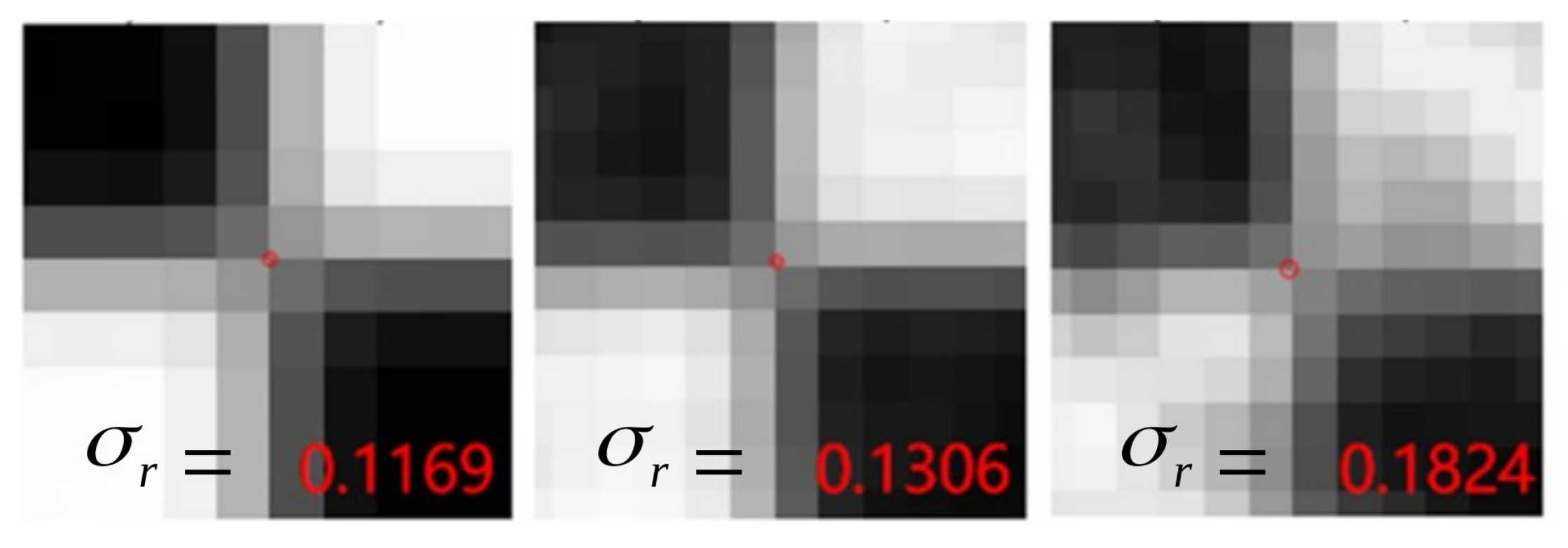
so that features with larger localization uncertainty receive lower weights. Figure 8 illustrates the point-dependent uncertainty radii used in the optimization.

In the physical experiments, feature-reliability scales are calculated before pose optimization. The checkerboard and aircraft extraction scripts use refinement half-windows of 31 and 21 pixels, respectively. The empirical scales enter WCS as fixed relative uncertainty weights. The pose refinement is evaluated conditional on these feature coordinates and scales; the uncertainty-assignment and covariance-sensitivity comparisons characterize how the choice of weights affects the result.

The simulation weighting benchmark uses the absolute difference between the clean and perturbed coordinates as a realized-error, or oracle, scale. The covariance-model experiments use the specified localization-noise-and-turbulence parameters to construct diagonal and full covariance matrices. These two weighting conditions assess the effects of pointwise precision and spatial correlation, respectively. A coordinate variance below $10^{-5}$ pixel² is assigned unit precision in the pointwise benchmark. These benchmarks use clean coordinates or a prescribed covariance model, respectively.

Pointwise inverse variances approximate the precision matrix by independent coordinate contributions. Atmospheric image motion, common blur, and calibration residuals can also produce cross-feature and cross-coordinate correlation. For a joint covariance matrix, whitening is defined by

$$\mathsf{\Sigma }={\mathbf{L}}_{\Sigma }{\mathbf{L}}_{\Sigma }^{\mathrm{T}}, \tilde{\mathbf{r}}={\mathbf{L}}_{\Sigma }^{-1}\mathbf{r}, \tilde{\mathbf{J}}={\mathbf{L}}_{\Sigma }^{-1}\mathbf{J}.$$

(27)

For the controlled comparisons in Section 3.2.6, whitening is applied to both the residual and Jacobian before centering and column scaling. These operations generally do not commute. Centered and mean components are retained together so that the local weighted objective is preserved.

A scalar factor $\alpha$ adjusts the nominal precision level

$${{\mathbf{W}}^{\prime }}_i=\alpha {\mathbf{W}}_i.$$

(28)

The nominal precision scale is $\alpha =1$, and $\alpha =3$ and 9 evaluate sensitivity. For uniform rescaling, substituting $\mathbf{W}\left(\alpha \right)=\alpha \mathbf{W}\left(1\right)$ into the normalized LM equations and dividing by $\alpha$ gives

$$\left[{\mathbf{J}}^{\prime \mathrm{T}}\mathbf{W}(1){\mathbf{J}}^{\prime }+{\displaystyle \frac{\lambda }{\alpha }}{\mathbf{I}}_6\right]{\mathbf{d}}^{\prime }=-{\mathbf{J}}^{\prime \mathrm{T}}\mathbf{W}(1)\mathbf{r}.$$

(29)

A global precision scale therefore changes the effective damping while preserving the undamped weighted least-squares minimizer. Section 3.2.3 and Section 3.2.5 examine pointwise uncertainty assignment and uniform covariance rescaling.

For the whitened residual $e=L_{\mathsf{\Sigma }}^{-1}r$ and Jacobian $B=L_{\mathsf{\Sigma }}^{-1}J$, define $A_c=CB{D}^{-1}$, $a_0=\sqrt{m}\hspace{0.17em}\overline{B}{D}^{-1}$, and $e_0=\sqrt{m}\hspace{0.17em}\overline{e}$, where $m=2n$ and bars denote means over the m residual coordinates. The normalized weighted LM update is

$$d_k^{*}=-{\left(A_c^T{A}_c+a_0^T{a}_0+\lambda I_6\right)}^{-1}\left(A_c^{T}Ce+a_0^T{e}_0\right).$$

(30)

Finally, the update is transformed back to the original parameter scale: the mean terms give $A_c^T{A}_c+a_0^T{a}_0=D^{-1}{B}^{T}B{D}^{-1}$ and $A_c^{T}Ce+a_0^T{e}_0=D^{-1}{B}^{T}e$, retaining the full objective gradient.

$${\mathbf{d}}_k={\mathbf{D}}^{-1}{{\mathbf{d}}^{\prime }}_k, \mathbf{D}=\mathrm{d}\mathrm{i}\mathrm{a}\mathrm{g}\left(s_1,s_2,\dots ,s_6\right).$$

(31)

The diagonal scale and current-pose Jacobian are recomputed at each linearization. Centered-column norms are bounded below by $\mathrm{m}\mathrm{a}\mathrm{x}({10}^{-12}{∥B_{:q}∥}_2,{10}^{-300})$. The Rodrigues-vector and translation coordinates are updated additively, followed by Rodrigues conversion to a rotation matrix. The augmented least-squares system is solved by SVD. Termination records distinguish the gradient criterion, a small step and the iteration limit.

3. Results

3.1. Experimental Settings and Evaluation Metrics

The proposed approach is compared with DLT, EPnP, RPnP, conventional LM refinement initialized by RPnP (RPnP-LM), central-normalization refinement (RPnP-CS), and weighted central normalization at three precision scales (RPnP-WCS-1C, RPnP-WCS-3C, and RPnP-WCS-9C). Each simulation condition contains 100 paired trials. Competing refinements receive the same image observations and RPnP initialization within each trial.

Rotation and translation errors were evaluated separately. The rotation-matrix error is

$$e_{\mathrm{r}\mathrm{o}\mathrm{t}}={∥{\mathbf{R}}_{\mathrm{e}\mathrm{s}\mathrm{t}}{\mathbf{R}}_{\mathrm{g}\mathrm{t}}^T-{\mathbf{I}}_3∥}_F,$$

(32)

and the translation error is

$$e_{\mathrm{t}\mathrm{r}\mathrm{a}\mathrm{n}}={∥{\mathbf{t}}_{\mathrm{e}\mathrm{s}\mathrm{t}}-{\mathbf{t}}_{\mathrm{g}\mathrm{t}}∥}_2.$$

(33)

For the noise-and-turbulence comparisons, the per-point reprojection RMS is

$$e_{\mathrm{i}\mathrm{m}\mathrm{g}}=\sqrt{{\displaystyle \frac{1}{n}}{\displaystyle \sum _{i=1}^n}\left[({\widehat{x}}_i-x_i{)}^2+({\widehat{y}}_i-y_i{)}^2\right]}.$$

(34)

The rotation and translation metrics use the same definitions across the simulation comparisons. Section 3.2.2 reports the aggregate reprojection statistic, and Section 3.2.5 reports the per-point RMS above.

3.2. Simulation Results

The simulations use focal lengths of 100, 1000, and 10,000 mm with planar and three-dimensional targets.

Table 1. Camera focal lengths and target geometry used in the simulations. The X/Y extent is the full target span along each image-plane direction.

Target	Focal Length (mm)	Range (km)	Full X/Y Extent (m)	Depth Extent (m)
2D	100	15	2160	0.0
2D	1000	600	10,800	0.0
2D	10,000	15,000	21,600	0.0
3D	100	10	2160	467.5
3D	1000	300	10,800	2329.8
3D	10,000	10,000	21,600	4755.2

lists the object ranges and full target extents. These six configurations examine numerical conditioning at different far-field scales. A fixed-target distance sweep evaluates angular shrinking, and the noise-and-turbulence experiments evaluate measurement disturbances under the same camera and target configurations.

The principal point is (4344, 2896) pixels, the image size is 8688 × 5792 pixels, and the pixel pitch is 36/8688 mm. The camera model has zero skew and zero lens distortion. Each geometry and noise level contains 100 pose/noise realizations with 100 feature points.

3.2.1. Pose Measurement Accuracy

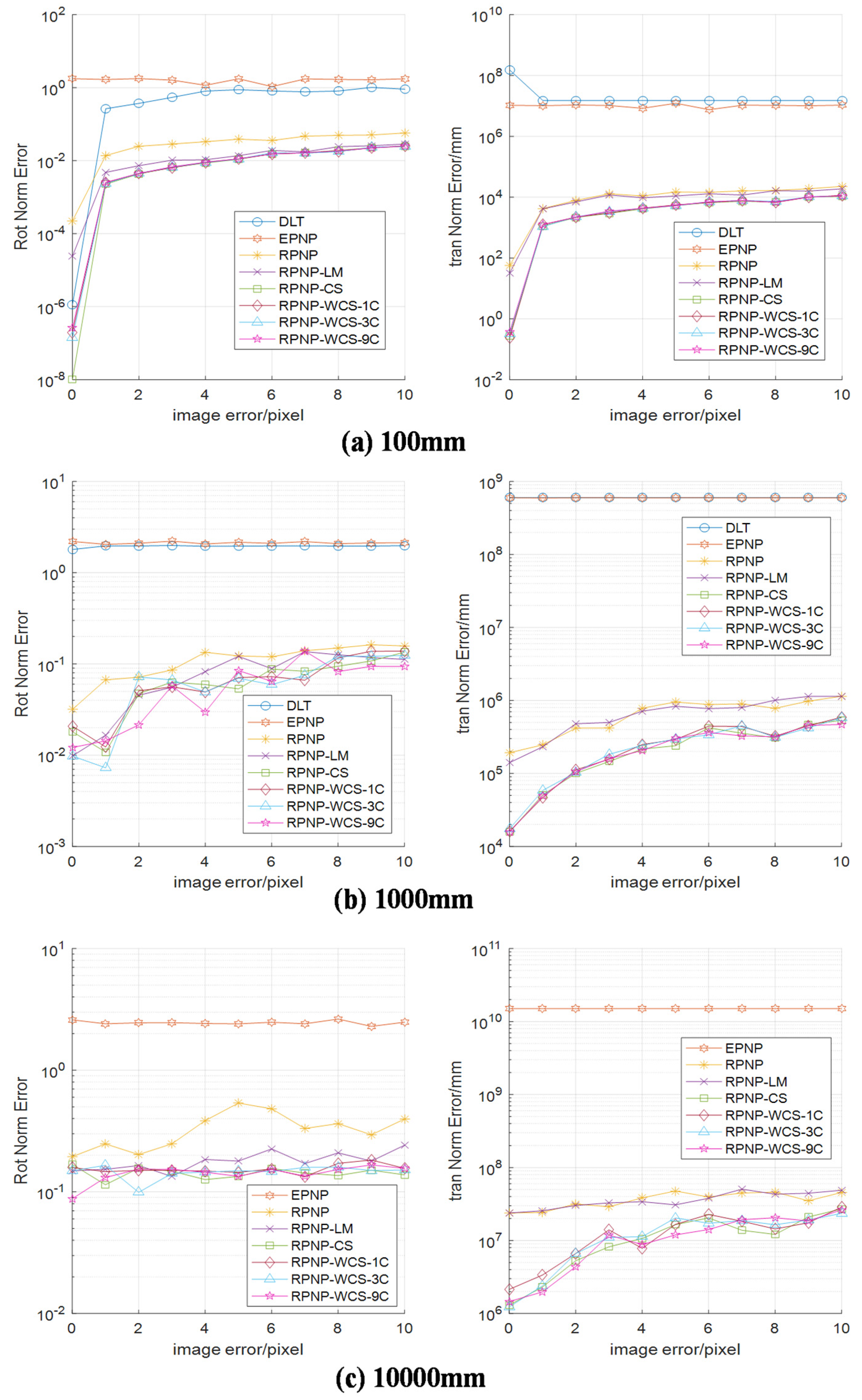
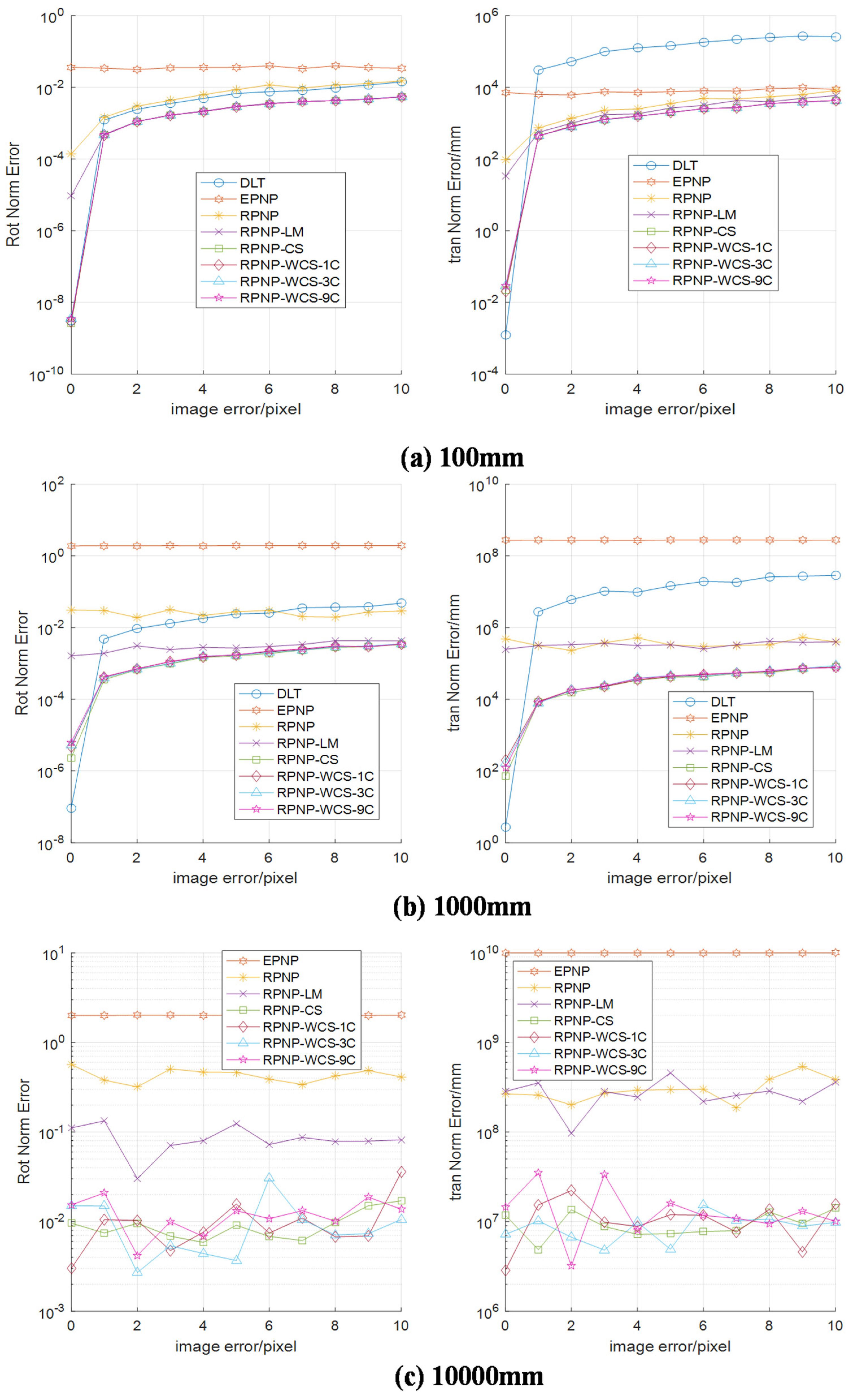
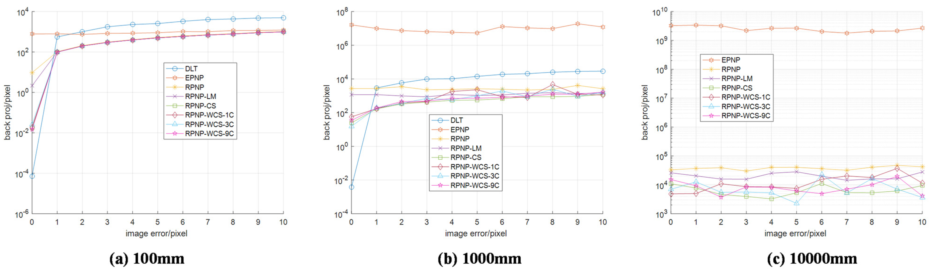
Figure 9 and Figure 10 compare pose errors for planar and three-dimensional targets at three focal lengths. RPnP provides a stable initialization, and nonlinear refinement improves its accuracy. For the three-dimensional target at 10,000 mm and 1-pixel noise, CS reduces robust-RMS rotation and translation errors by 94.4% and 98.6% relative to RPnP-LM. Section 3.2.3 and Section 3.2.5 examine geometry, initialization, and measurement disturbances.

At 2-pixel noise and a 10,000 mm focal length, the planar-target median $e_{\mathrm{r}\mathrm{o}\mathrm{t}}$ values are 0.1079, 0.0954, and 0.0524 for RPnP-LM, RPnP-CS, and WCS-3C, respectively. Relative translation error is the translation norm error divided by the ground-truth translation norm and expressed as a percentage. Its median values are 0.1360%, 0.0257%, and 0.0260%, with pose-threshold failure rates of 18%, 12%, and 14%. A pose-threshold failure exceeds 10° in geodesic rotation error or 2% in relative translation error. Central normalization substantially reduces the translation error in this weak-perspective geometry.

For the three-dimensional target under the same condition, the median $e_{\mathrm{r}\mathrm{o}\mathrm{t}}$ values are 0.0088, 0.0019, and 0.0015, and the median relative translation errors are 0.4564%, 0.0164%, and 0.0126%. The respective pose-threshold failure rates are 25%, 13%, and 15%. Both normalized variants improve pose accuracy, with WCS-3C giving the lowest median errors in this condition.

3.2.2. Reprojection Error

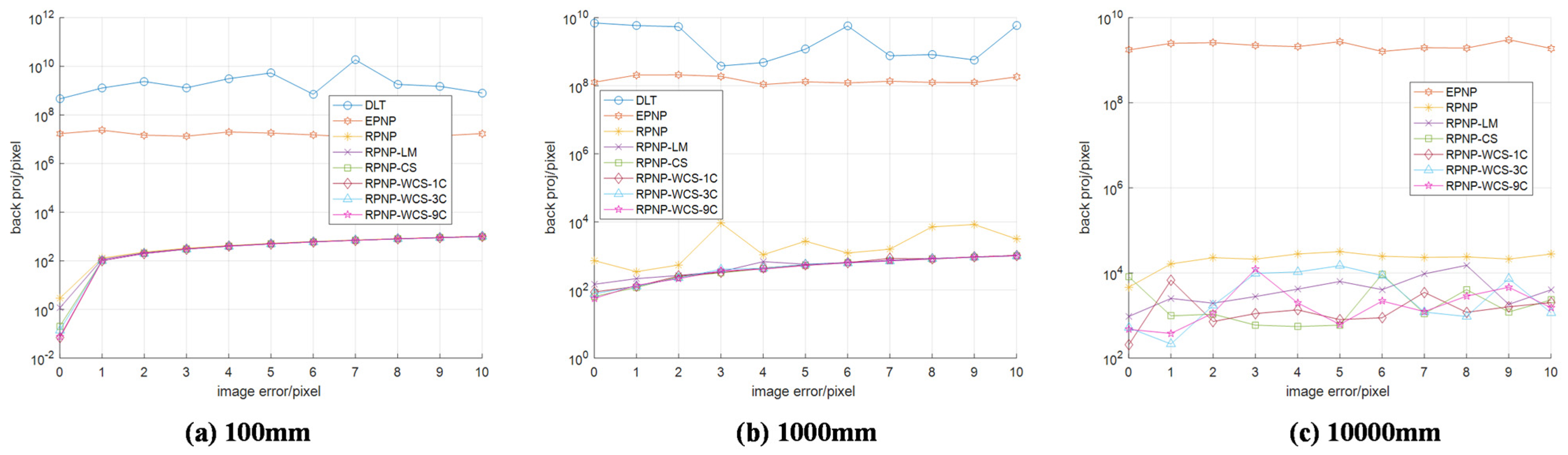
Figure 11 and Figure 12 show the image reprojection errors for planar and three-dimensional objects. Because all nonlinear variants minimize a reprojection objective, their final image-space errors are closer to one another than their pose-parameter errors. Nevertheless, the centrally normalized solutions remain stable as the focal length increases, indicating that the improved pose accuracy is not obtained at the expense of poorer image consistency.

3.2.3. Sensitivity, Ablation, and Converged-Hessian Analysis

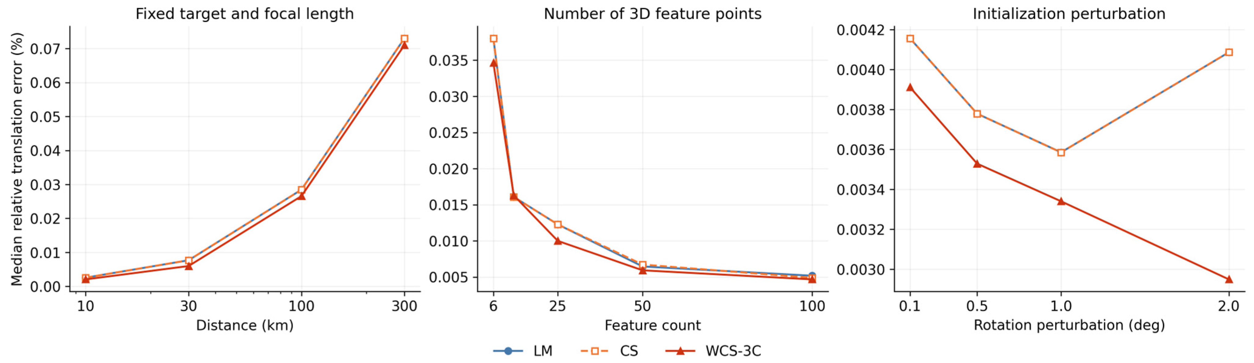
For a fixed target with a full X/Y span of 2160 m and a 100 mm focal length, increasing distance from 10 to 300 km raises the WCS-3C median relative translation error from 0.0021% to 0.0710%, showing the effect of angular shrinking. Increasing the three-dimensional feature count from 6 to 100 lowers this error from 0.0346% to 0.0047%. Across initialization perturbations of 0.1° to 2.0°, WCS-3C maintains a median error below 0.004% with zero pose-threshold failures. The heteroscedastic noise levels are 0.5, 1.0, and 0.75 pixels for these three tests, respectively. LM, CS, and WCS are applied sequentially with the stopping tolerances used in

Table 2. Controlled component ablation at 10,000 mm focal length and 2-pixel image noise (100 paired trials per geometry).

Geometry	Variant	${\mathit{e}}_{\mathbf{r}\mathbf{o}\mathbf{t}}$ Median	${\mathit{e}}_{\mathbf{t}\mathbf{r}\mathbf{a}\mathbf{n}}$ (%) Median	Mean Iterations	Failure (%)
2D	LM	0.0477	0.0184	10.97	12
2D	C	0.0477	0.0367	18.78	12
2D	S	0.0122	0.0120	5.47	11
2D	CS	0.0122	0.0122	7.07	10
2D	CS-GN	0.1438	0.1343	1.00	100
2D	WCS-3C	0.0224	0.0081	10.28	17
3D	LM	0.0011	0.0075	10.87	20
3D	C	0.0013	0.0124	21.23	20
3D	S	0.0010	0.0060	3.93	0
3D	CS	0.0010	0.0060	6.08	0
3D	CS-GN	0.1623	0.8995	1.00	100
3D	WCS-3C	0.0018	0.0101	18.98	9

Errors are medians over 100 paired trials. Failure includes nonconvergence, geodesic rotation error above 10°, or relative translation error above 2%. C, S, and CS denote centering, scaling, and their combination; CS-GN removes damping. Iteration counts exclude RPnP initialization.

. WCS uses the prescribed coordinate variances and $\alpha =3$.

The component ablation uses the 10,000 mm, 2-pixel observations and a common RPnP initialization for every variant. Each geometry contains 100 paired trials. The common stopping rule is a relative scaled-step tolerance of $10^{-10}$, an accepted relative objective reduction below $10^{-12}$, or 250 iterations. The comparison separates centering (C), column scaling (S), their combination (CS), LM damping, and uncertainty weighting. Figure 13 summarizes the distance, feature-count, and initialization tests.

Table 2 shows the contribution of each component. For the planar target, scaling reduces the median $e_{\mathrm{r}\mathrm{o}\mathrm{t}}$ and relative translation error from 0.0476 and 0.0184% for LM to 0.0122 and 0.0120%. CS gives 0.0122 and 0.0123% and reduces the failure rate from 12% to 10%. For the three-dimensional target, the corresponding errors are 0.0011 and 0.0075% for LM, 0.0010 and 0.0060% for S, and 0.0010 and 0.0060% for CS; S and CS have zero failures. The accuracy improvement is mainly associated with column-scale balancing. CS-GN fails the common convergence test in all trials, demonstrating the role of damping in stabilizing this update. The controlled comparison in Section 3.2.6 complements these results with a common-initialization comparison using the complete weighted update.

The uncertainty perturbation tests distinguish global scale from relative assignment. In the planar case, multiplying every estimated $\sigma$ by 0.5 or 2 gives median rotation/relative-translation error values of 0.0185/0.0086% and 0.0147/0.0067%, whereas permuting the pointwise values increases them to 0.0892/0.0661%. In the three-dimensional case, the corresponding values are 0.0015/0.0083%, 0.0009/0.0048%, and 0.0075/0.0520%. For $\alpha =1$, 3, and 9, the planar WCS failure rates are 15%, 17%, and 19%, and the three-dimensional rates are 8%, 9%, and 10%. Uniform rescaling mainly interacts with damping, while accurate feature-to-uncertainty correspondence has a stronger effect on accuracy. Reliable featurewise uncertainty estimates are needed to supply this correspondence for WCS, while CS provides the unweighted refinement.

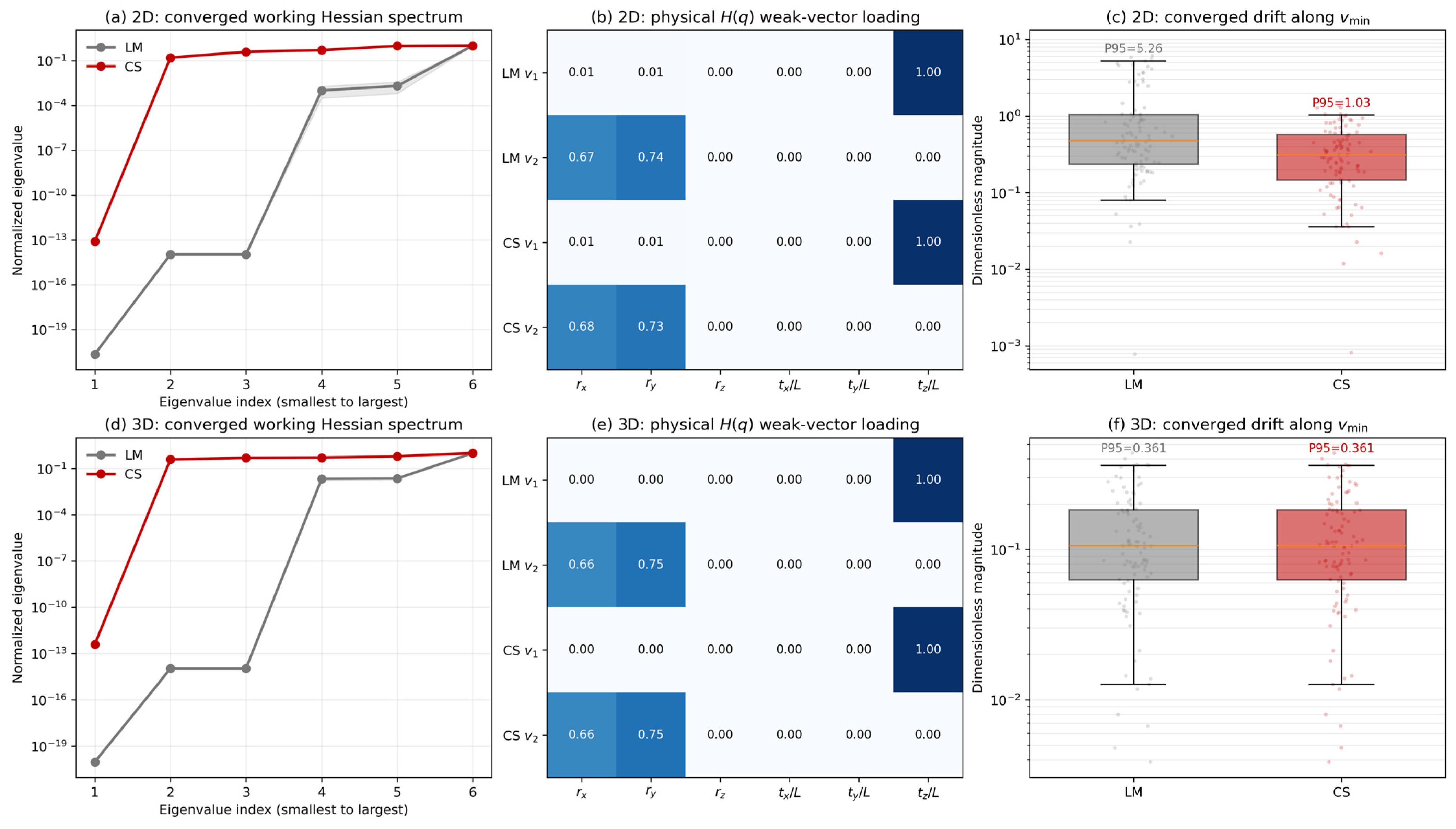
Weak modes are evaluated at each converged LM and CS estimate in the 10,000 mm, 2-pixel heteroscedastic-noise condition. With the Jacobian columns ordered as rotation followed by translation, the dimensionless pose and target scaling are

$$\mathbf{q}={\left[{\mathbf{r}}^{\mathrm{T}},(\mathbf{t}/L{)}^{\mathrm{T}}\right]}^{\mathrm{T}}, \mathbf{S}=\mathrm{d}\mathrm{i}\mathrm{a}\mathrm{g}({\mathbf{I}}_3,L{\mathbf{I}}_3),$$

(35)

Here, $\mathbf{r}$ is the Rodrigues rotation vector and $L$ is the target root-mean-square radius. The target-scale-normalized Jacobian and information matrix are

$${\mathbf{J}}_q=\mathbf{J}\mathbf{S}, {\mathbf{H}}_q={\displaystyle \frac{1}{2n}}{\mathbf{J}}_q^{\mathrm{T}}{\mathbf{J}}_q.$$

(36)

The unit eigenvector associated with the smallest eigenvalue defines the weak direction and its pose-error component:

$${\mathbf{H}}_q{\mathbf{v}}_{\mathrm{m}\mathrm{i}\mathrm{n}}={\lambda }_{\mathrm{m}\mathrm{i}\mathrm{n}}\left({\mathbf{H}}_q\right){\mathbf{v}}_{\mathrm{m}\mathrm{i}\mathrm{n}}, d_{\mathrm{m}\mathrm{i}\mathrm{n}}=\left|{\mathbf{v}}_{\mathrm{m}\mathrm{i}\mathrm{n}}^{\mathrm{T}}\Delta \mathbf{q}\right|.$$

(37)

The normal matrices used by the two algorithms are evaluated as

$${\mathbf{H}}_{\mathrm{L}\mathrm{M}}={\mathbf{J}}^{\mathrm{T}}\mathbf{J}, {\mathbf{H}}_{\mathrm{C}\mathrm{S}}={\mathbf{J}}^{\prime \mathrm{T}}{\mathbf{J}}^{\prime }.$$

(38)

These matrices characterize numerical conditioning, while the dimensionless matrix characterizes the geometry of weak pose directions. All statistics use 100 paired trials per target geometry.

Figure 14 confirms that the smallest-eigenvalue direction is dominated by normalized depth translation, $q_6={\displaystyle \frac{t_z}{L}}$. For the planar target, the median value of $\left|{v_{\mathrm{m}\mathrm{i}\mathrm{n}}}_6\right|$ is 0.99995 for LM and 0.99996 for CS; for the three-dimensional target, it is 0.99999 for both methods. The second-smallest mode is dominated by coupled $r_x$–$r_y$ rotation. The physical near-null direction remains essentially unchanged after central normalization.

The median spectral condition numbers of the algorithmic normal matrices are ${\kappa }_2\left(H_{\mathrm{L}\mathrm{M}}\right)=4.49\times {10}^{20}$ and ${\kappa }_2\left(H_{\mathrm{C}\mathrm{S}}\right)=1.27\times {10}^{13}$ for the planar target, and ${\kappa }_2\left(H_{\mathrm{L}\mathrm{M}}\right)=1.06\times {10}^{20}$ and ${\kappa }_2\left(H_{\mathrm{C}\mathrm{S}}\right)=2.57\times {10}^{12}$ for the three-dimensional target. These values compare numerical conditioning in the corresponding solver coordinates, whereas the target-scale-normalized matrix characterizes physical observability.

For the planar target, the LM-to-CS changes are $\mathrm{m}\mathrm{e}\mathrm{d}\mathrm{i}\mathrm{a}\mathrm{n}\left(d_{\mathrm{m}\mathrm{i}\mathrm{n}}\right)=0.472\to 0.309$, $P_{95}\left(d_{\mathrm{m}\mathrm{i}\mathrm{n}}\right)=5.26\to 1.03$, and $\mathrm{m}\mathrm{a}\mathrm{x}\left(d_{\mathrm{m}\mathrm{i}\mathrm{n}}\right)=8.29\to 1.36$. These correspond to reductions of 34.4% in the sample median and 80.5% in the 95th percentile. For the three-dimensional target, the rounded median and 95th percentile remain 0.106 and 0.361, respectively, for both methods. The benefit is therefore concentrated in suppressing the upper tail of weak-mode drift for the more ambiguous planar geometry.

3.2.4. Runtime Analysis

The runtime evaluation uses MATLAB R2016 on Windows 10 with an Intel Core i7-10510U processor.

Table 3. Mean runtime of the evaluated methods over 100 repeated trials (ms).

Focal Length (mm)	DLT	EPnP	RPnP	RPnP-LM	RPnP-CS	RPnP-WCS
100	14.9	15.5	18.0	76.7	161.9	461.4
1000	15.5	15.4	14.3	71.4	144.2	403.3
10,000	—	16.5	15.4	78.2	177.5	309.7

An em dash indicates that a valid DLT result was not obtained for the 10,000 mm case. In this near-affine limit, the DLT linear system loses effective numerical rank.

reports the mean of 100 runs for each focal length. RPnP-LM contains one refinement stage, RPnP-CS applies LM followed by CS, and WCS applies LM, CS, and WCS sequentially, with at most 1000 iterations per stage. The additional refinement stages and matrix operations increase the total runtime. Under the common stopping rule in Table 2, the mean final-stage iteration counts for the planar/three-dimensional targets are 10.97/10.87 for LM, 18.78/21.23 for C, 5.47/3.93 for S, 7.07/6.08 for CS, and 10.28/18.98 for WCS-3C. These counts identify the contribution of each refinement component to the computational cost.

3.2.5. Robustness to Localization Noise and Atmospheric Turbulence

The robustness experiments use the six configurations in Table 1 and localization-noise levels from 0 to 10 pixels. Atmospheric displacement is applied to the image coordinates. Turbulence is evaluated both alone and in combination with 1-pixel localization noise. Each condition contains 100 trials with 100 feature points, and all methods receive the same perturbed observations within each trial. The random seed is 20,260,905, with paired realizations across turbulence strengths.

Atmospheric image motion is modeled by a single thin layer with aperture-averaged von Kármán angle-of-arrival covariance [35,36]. The wavelength is ${\lambda }_{\mathrm{w}}=550$ nm, the outer scale is $L_0=25$ m, the inner scale is $l_0=0.01$ m, and the effective layer distance is 1000 m. The simulated aperture ratio is f/10, giving diameters of 0.01, 0.1, and 1 m for the three focal lengths. Fried parameters $r_0=0.20$, 0.10, and 0.05 m represent increasing turbulence strength. At a focal length of 10,000 mm, the corresponding marginal coordinate standard deviations are 1.458, 2.598, and 4.629 pixels.

The phase power spectrum is

$${\Phi }_{\phi }(\nu )=0.023 r_0^{-5/3}\mathrm{e}\mathrm{x}\mathrm{p}\left[-{\left({\displaystyle \frac{\nu }{{\nu }_m}}\right)}^2\right]{\left({\nu }^2+L_0^{-2}\right)}^{-11/6},$$

(39)

where $\nu$ is spatial frequency and the inner-scale cutoff is

$${\nu }_m={\displaystyle \frac{5.92}{2\pi l_0}}.$$

(40)

For a circular aperture of diameter $D$, the aperture-averaging transfer function is

$$A_D(\nu )={\displaystyle \frac{2J_1\left(\pi D\nu \right)}{\pi D\nu }},$$

(41)

where $J_1$ is the first-order Bessel function. The angle-of-arrival covariance at footprint separation $\mathsf{\rho }$ is

$$K_{ab}(\mathsf{\rho })={\lambda }_{\mathrm{w}}^2{\int }_{{\mathbb{R}}^2}{\nu }_a{\nu }_b{\Phi }_{\phi }(\Vert \mathsf{\nu }\Vert )A_D^2(\Vert \mathsf{\nu }\Vert )\mathrm{c}\mathrm{o}\mathrm{s}\left(2\pi {\mathsf{\nu }}^{\mathrm{T}}\mathsf{\rho }\right) {\mathrm{d}}^2\mathsf{\nu }.$$

(42)

Indices $a,b\in \{x,y\}$ identify the two image coordinates. Let ${\mathsf{\rho }}_i$ denote the feature-ray footprint in the effective layer and let $f_a$ be the focal length in pixels along coordinate $a$. The image-displacement covariance and observation model are

$$[{\mathsf{\Sigma }}_{\mathrm{a}\mathrm{t}\mathrm{m}}{]}_{(i,a),(j,b)}=f_a{f}_b{K}_{ab}({\mathsf{\rho }}_i-{\mathsf{\rho }}_j),$$

(43)

$${\mathsf{ϵ}}_{\mathrm{a}\mathrm{t}\mathrm{m}}\sim \mathcal{N}(\mathbf{0},{\mathsf{\Sigma }}_{\mathrm{a}\mathrm{t}\mathrm{m}}), {\mathbf{p}}_{\mathrm{o}\mathrm{b}\mathrm{s}}={\mathbf{p}}_{\mathrm{l}\mathrm{o}\mathrm{c}}+{\mathsf{ϵ}}_{\mathrm{a}\mathrm{t}\mathrm{m}}.$$

(44)

The $2n\times 2n$ covariance includes inter-feature and cross-coordinate terms. The vector ${\mathbf{p}}_{\mathrm{l}\mathrm{o}\mathrm{c}}$ contains the localization-noise observations, and the correlated atmospheric displacement is applied before pose estimation.

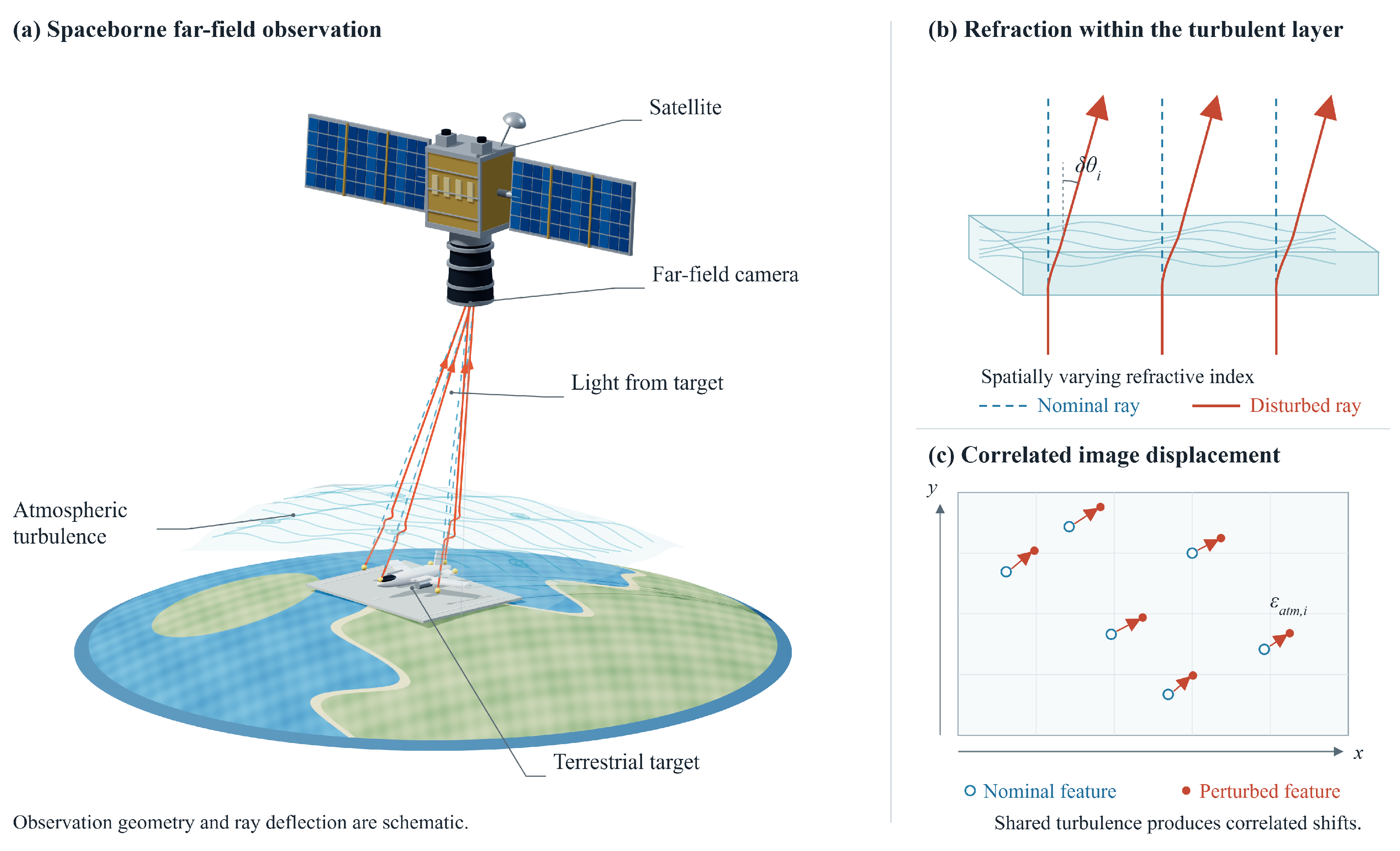
Figure 15 illustrates the formation of atmospheric image motion in a conceptual spaceborne observation geometry. Light from the target traverses a turbulent atmospheric layer before reaching the camera. Spatial variations in refractive index perturb the arrival directions, and neighboring feature rays experience correlated angular deviations. The simulation represents this effect through the joint covariance of image-coordinate displacements.

The method-comparison curves evaluate the sequential RPnP, LM, CS, and WCS stages. Table 2 and Section 3.2.1, Section 3.2.2, Section 3.2.3, Section 3.2.4 and Section 3.2.5 describe this finite-budget pipeline. The controlled comparisons in Section 3.2.6 evaluate Equation (30) from common RPnP initializations with a current-pose Jacobian, consistent whitening, and the complete centered and mean components.

The robust-RMS procedure uses $m_e=\mathrm{m}\mathrm{e}\mathrm{d}\mathrm{i}\mathrm{a}\mathrm{n}\left(e_i\right)$ and $s_e=\mathrm{m}\mathrm{e}\mathrm{d}\mathrm{i}\mathrm{a}\mathrm{n}\left|e_i-m_e\right|/0.6745$, rejecting $\left|e_i-m_e\right|>3s_e$. At most $\mathrm{f}\mathrm{l}\mathrm{o}\mathrm{o}\mathrm{r}\left(0.2N_f\right)$ finite observations with the largest deviations are excluded; ties follow record order. Nonfinite results are counted separately, and capped or nonstationary finite results remain in unfiltered summaries. The controlled comparison in Section 3.2.6 is unfiltered. Section 3.2.7 and Section 3.3.6 report the unfiltered statistics and actual exclusions.

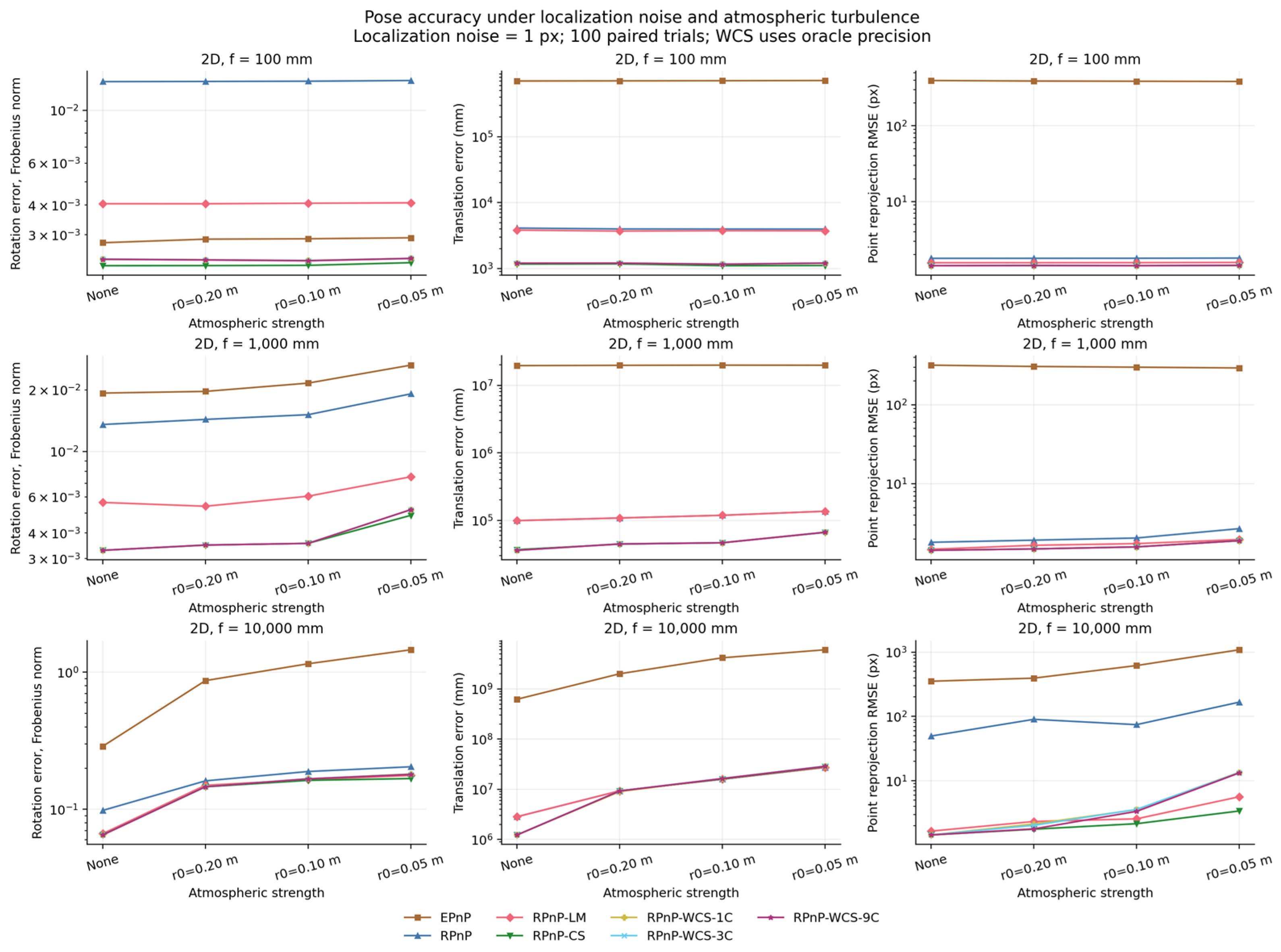
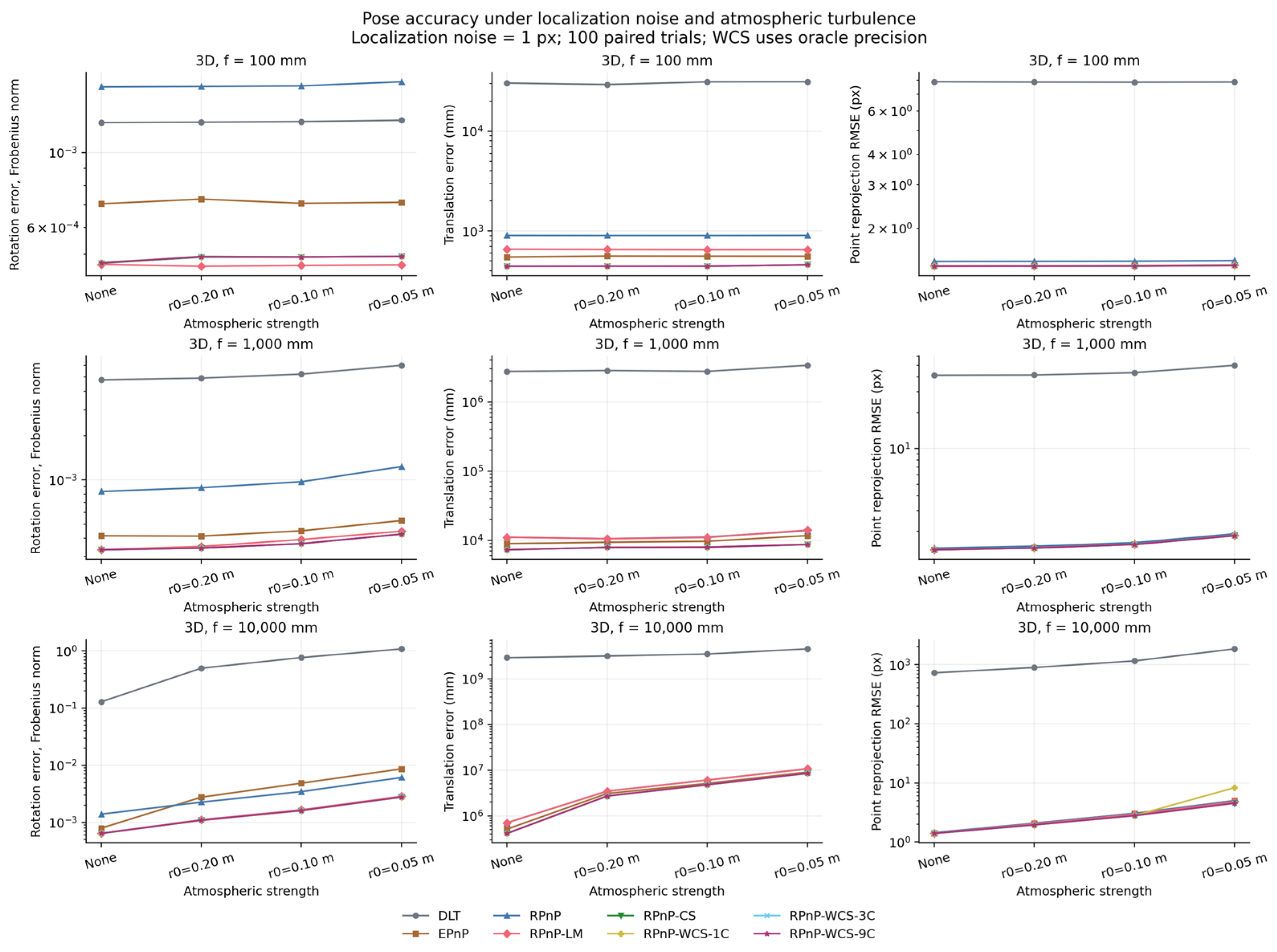
Figure 16 and Figure 17 show increased image residuals and pose errors under atmospheric disturbance. At $r_0=0.10$ m in the 10,000 mm three-dimensional sequential comparison, CS reduces robust-RMS rotation error from 0.0035 to 0.0016 and translation error from $6.086\times {10}^6$ to $4.810\times {10}^6$ mm relative to RPnP. Per-point reprojection RMS decreases from 3.033 to 2.790 pixels.

The translation benefit persists across the three turbulence strengths. For $r_0=0.20$, 0.10, and 0.05 m, CS reduces the robust-RMS translation error relative to RPnP-LM by 21.7%, 21.0%, and 20.6%, respectively. The CS and WCS curves nearly coincide at the representative condition, summarizing the performance of this sequential comparison. The WCS stage reaches the 1000-iteration limit in 56–57% of these trials. Section 3.2.6 reports termination statistics for the complete update in Equation (30).

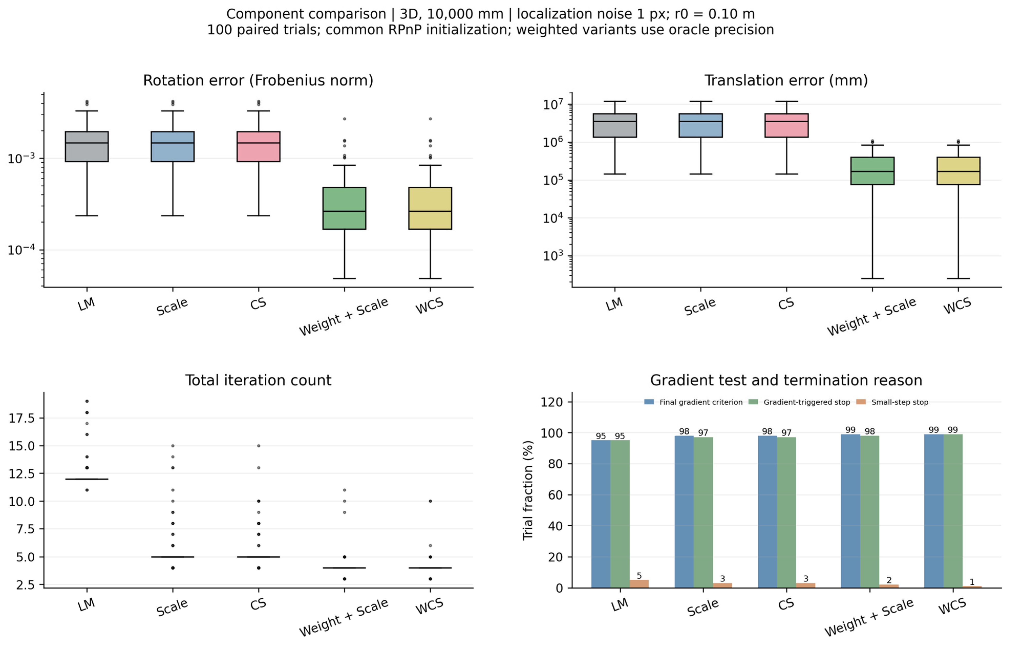
Figure 18 evaluates central normalization and uncertainty weighting under common observations and initialization. CS and scaling give nearly identical errors and a median of five iterations, compared with twelve for LM. WCS and the weighted scaling baseline both satisfy the final gradient criterion in 99% of trials. Section 3.2.6 and Section 3.2.7 give the paired comparisons and full error statistics. With the same gradient threshold, the mean-omission diagnostic gives 0/100 WCS gradient passes, compared with 99/100 for the complete update.

The controlled runs use an initial damping value of ${10}^{-5}$ and a factor-of-ten damping decrease or increase after accepted or rejected steps. The final column-normalized true-gradient threshold is ${10}^{-6}$. Gradient-triggered/small-step stops are 95/5 for LM, 97/3 for scaling and CS, 98/2 for Weight + Scale, and 99/1 for WCS. The final-pose gradient test is evaluated separately from the triggering stop.

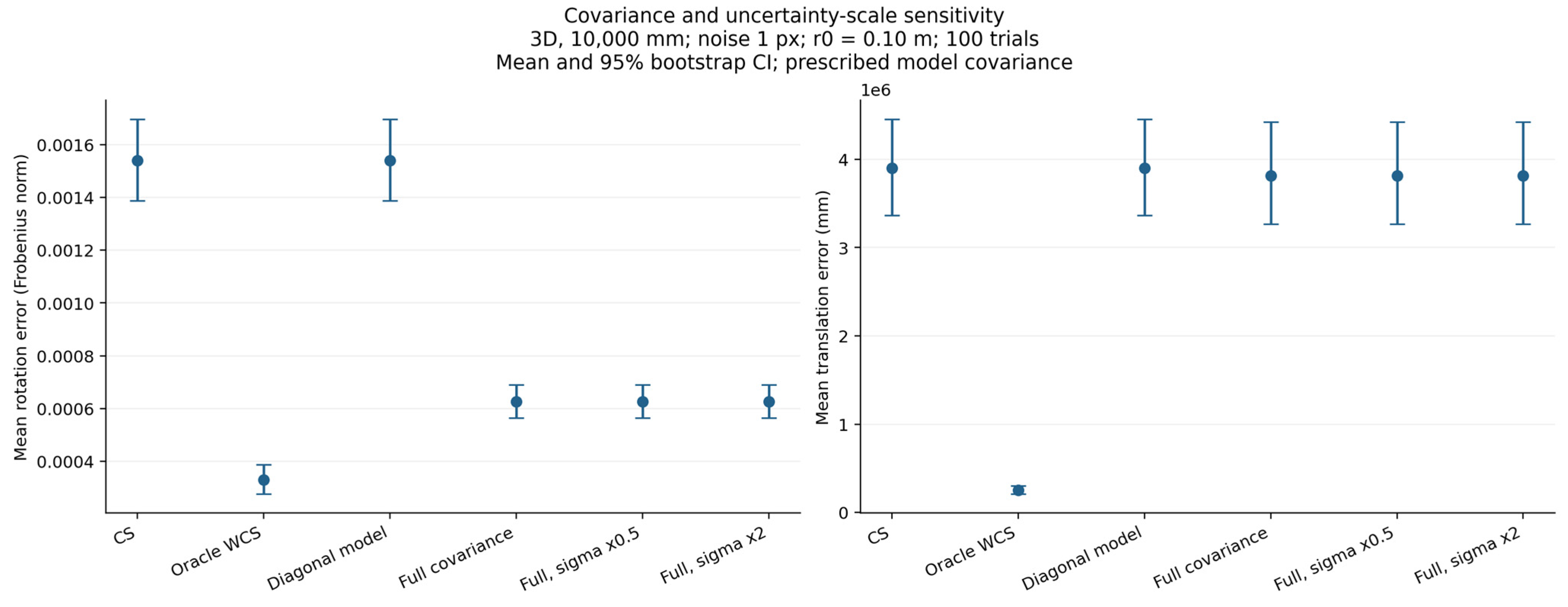
Figure 19 shows the influence of spatial covariance on pose refinement. The full model uses the joint covariance to whiten both the residual vector and Jacobian, while the diagonal model uses the marginal variances. The mean rotation error decreases from $1.539\times 10^{-3}$ for the diagonal model to $6.265\times 10^{-4}$ for the full model, a reduction of 59.3%. The paired mean difference is $-9.125\times 10^{-4}$, with a 95% confidence interval of $-1.093\times 10^{-3}$ to $-7.453\times 10^{-4}$. Accounting for spatial correlation therefore improves rotation estimation under the specified covariance model. The mean translation errors are statistically comparable.

Uniformly multiplying the assumed standard deviations by 0.5 or 2 produces essentially coincident results in Figure 19. A global covariance scale preserves the undamped weighted least-squares minimizer and largely cancels after column normalization. The rotation improvement is thus associated with the covariance structure. Weighted refinement evaluates image agreement in the covariance metric, so its unweighted reprojection RMS can differ from that of the unweighted fit.

3.2.6. Controlled Optimization and Covariance Results

Figure 18 and

Table 4. Termination and iteration statistics for the controlled Figure 18 comparison (100 trials per method).

Method	Final Gradient Pass	Gradient Stop	Small-Step Stop	Cap	Median Iterations
LM	95	95	5	0	12
Scale	98	97	3	0	5
CS	98	97	3	0	5
Weight + Scale	99	98	2	0	4
WCS	99	99	1	0	4

and

Table 5. Unfiltered mean pose errors and paired differences in Figure 18. Rotation error is the dimensionless Frobenius norm; translation is in mm.

Method or Paired Difference	Mean Rotation Error	Mean Translation Error (mm)
LM	0.0015	3,900,527.3919
Scale	0.0015	3,900,527.4002
CS	0.0015	3,900,527.3989
Weight + Scale	0.0004	272,346.9054
WCS	0.0004	272,346.9144
CS minus Scale	−1.5675 × 10−12	−0.0013
WCS minus Weight + Scale	3.2813 × 10−12	0.0090

use the same 100 observations and RPnP initializations for every method, with a common 1000-iteration budget. The final-pose gradient test and the event triggering termination are reported separately. All 500 outputs are finite, and no run reaches the iteration cap.

CS and Scale give comparable pose estimates in this comparison. The oracle-weighted variants give smaller pose errors under the known realized feature-reliability inputs. The paired differences in Table 5 summarize matched trials.

Table 6. Geometry comparison with common observations, initializations and iteration limits.

Geometry	Method	Median Rotation	Median Translation (%)	Mean Iterations	Gradient Pass	Pose Failures	Caps
Planar	LM	0.0661	0.0151	33.4000	82	8	5
Planar	Scale	0.0598	0.0125	7.3000	98	8	0
Planar	CS	0.0598	0.0125	7.3100	99	8	0
Planar	WCS-3C	0.0404	0.0018	7.6000	100	8	0
3D	LM	0.0010	0.0057	12.3900	95	0	0
3D	Scale	0.0010	0.0057	4.4400	97	0	0
3D	CS	0.0010	0.0057	4.3400	98	0	0
3D	WCS-3C	0.0002	0.0008	4.2000	98	0	0

uses 100 paired trials per geometry at a 10,000 mm focal length and 2-pixel noise, with a common 250-iteration budget. Pose failure denotes a rotation error above 10 degrees, a relative translation error above 2%, or an invalid pose. Rotation medians use the dimensionless Frobenius error.

Table 7. Prescribed covariance and global-scale comparison (100 trials per condition).

Covariance Model	Mean Rotation	Mean Translation (mm)	Gradient Pass	Caps
Diagonal	0.0015	3,900,527.4069	99	0
Full	0.0006	3,630,884.9470	99	0
Full; std × 0.5000	0.0006	3,630,884.9510	95	0
Full; std × 2	0.0006	3,630,884.9423	100	0

reports the prescribed covariance and global-scale comparison for the same 100 trials per condition.

Full covariance reduces mean rotation error by 59.3356% relative to diagonal covariance. Multiplying all full-model standard deviations by 0.5000 or 2 leaves the displayed pose errors nearly unchanged; the absolute gradient threshold gives different pass counts for the differently scaled precision models.

The centered and mean decomposition preserves the scaled local objective. Across the 100 Figure 18 linearizations, the maximum relative Gram-matrix and right-hand-side identity errors are 1.0015 × 10⁻¹⁵ and 3.3118 × 10⁻¹⁵, respectively. These comparisons characterize central normalization and uncertainty weighting under the stated geometries and weighting inputs.

3.2.7. Unfiltered Errors and Trial Accounting

Table 8. Filtered and unfiltered Figure 18 pose errors and actual exclusions.

Method	Rotation F	Rotation U	nR	Translation F (mm)	Translation U (mm)	nt
LM	0.0017	0.0017	2	4,809,468.9142	4,809,468.9142	0
Scale	0.0017	0.0017	2	4,809,468.9171	4,809,468.9171	0
CS	0.0017	0.0017	2	4,809,468.9162	4,809,468.9162	0
Weight + Scale	0.0004	0.0005	7	304,882.0921	371,912.0958	6
WCS	0.0004	0.0005	7	304,882.1097	371,912.1094	6

and

Table 9. Figure 18 tail errors and per-point reprojection RMS; n_P denotes reprojection exclusions.

Method	Rotation P95	Translation P95 (mm)	Reprojection F (px)	Reprojection U (px)	nP
LM	0.0028	8,505,148.6778	2.7744	2.7890	1
Scale	0.0028	8,505,148.6691	2.7744	2.7890	1
CS	0.0028	8,505,148.6691	2.7744	2.7890	1
Weight + Scale	0.0010	752,600.9728	3.5744	3.6332	2
WCS	0.0010	752,600.9728	3.5744	3.6332	2

report all 100 outputs per Figure 18 method. F and U denote filtered and unfiltered RMS; n_R and n_t are actual rotation and translation exclusion counts. Rotation errors are dimensionless and translation errors are in mm.

For each metric, filtering starts from finite observations and follows the median/MAD rule in Section 3.2.5. The 20% cap is applied after thresholding, retaining the largest deviations as exclusions. A zero MAD uses the same strict threshold inequality. Unfiltered summaries retain capped and nonstationary finite outputs; nonfinite outputs are counted separately. The geometry comparison contains five capped planar LM trials, which remain in its unfiltered error and failure summaries. Trial-level records identify observations, initial and final poses, gradient checks, accepted and rejected steps, termination reasons and paired method differences.

3.3. Scaled Physical Relative-Comparison Experiments

3.3.1. Experimental Setup

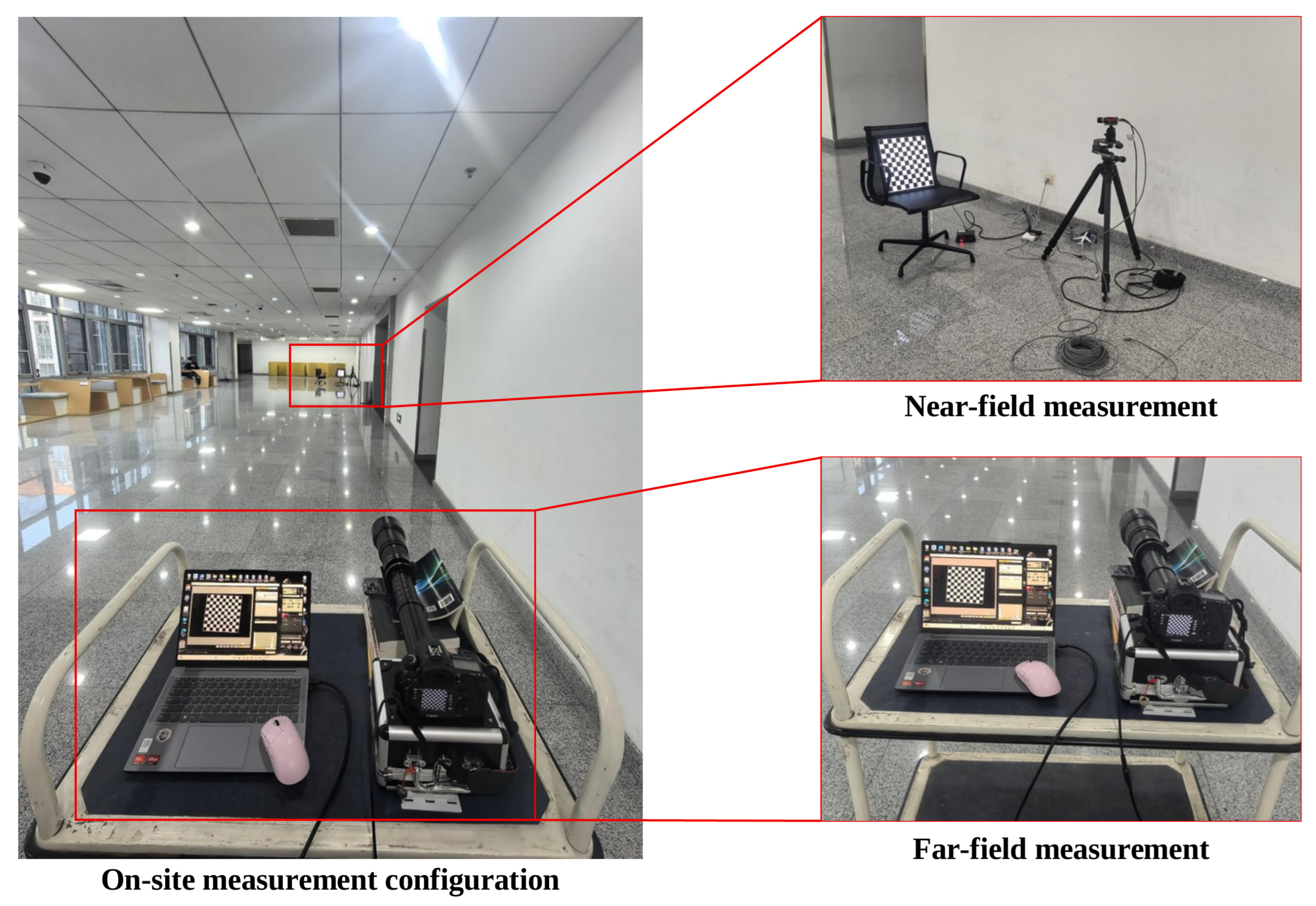
The physical setup uses near-field and far-field cameras to observe the same target, as shown in Figure 20. The far-field optical path spans approximately 40 m across the laboratory building, and the near-field camera is within 2 m of the target. A 10 × 10 checkerboard with 30 mm squares, an aircraft model, and a satellite model are measured. The approximate geometric scale is 1:1000. The setup evaluates relative-pose changes with long-focal-length imaging and controlled target placements.

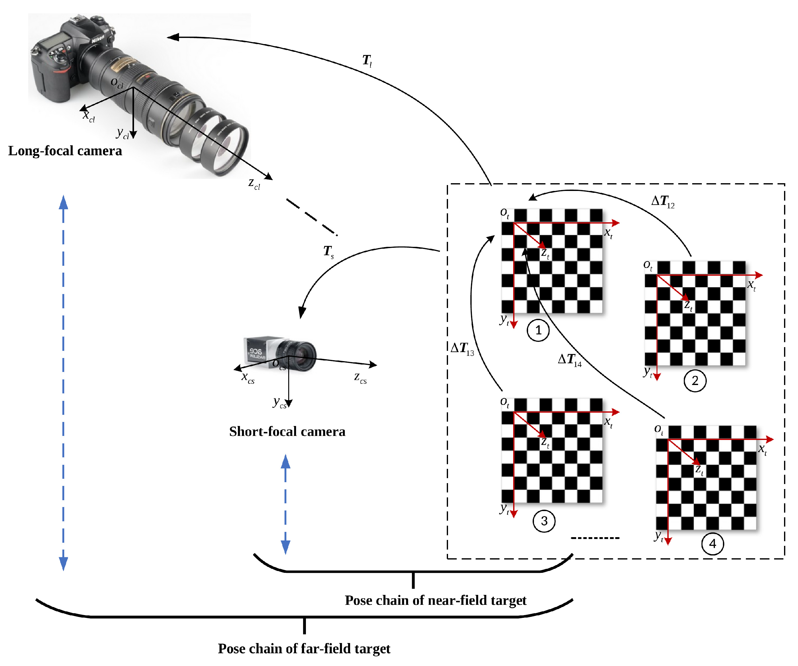
The near-field camera was an AVT GT2000NIR with a 17 mm lens. The far-field camera was a Canon EOS 5DS coupled to a 1300 mm focal-length optical system. Both cameras remained fixed while the target pose was changed. Images were acquired simultaneously, and the near-field measurements were used as reference values. Relative-pose changes between two target placements were compared through the transformation chain shown in Figure 21.

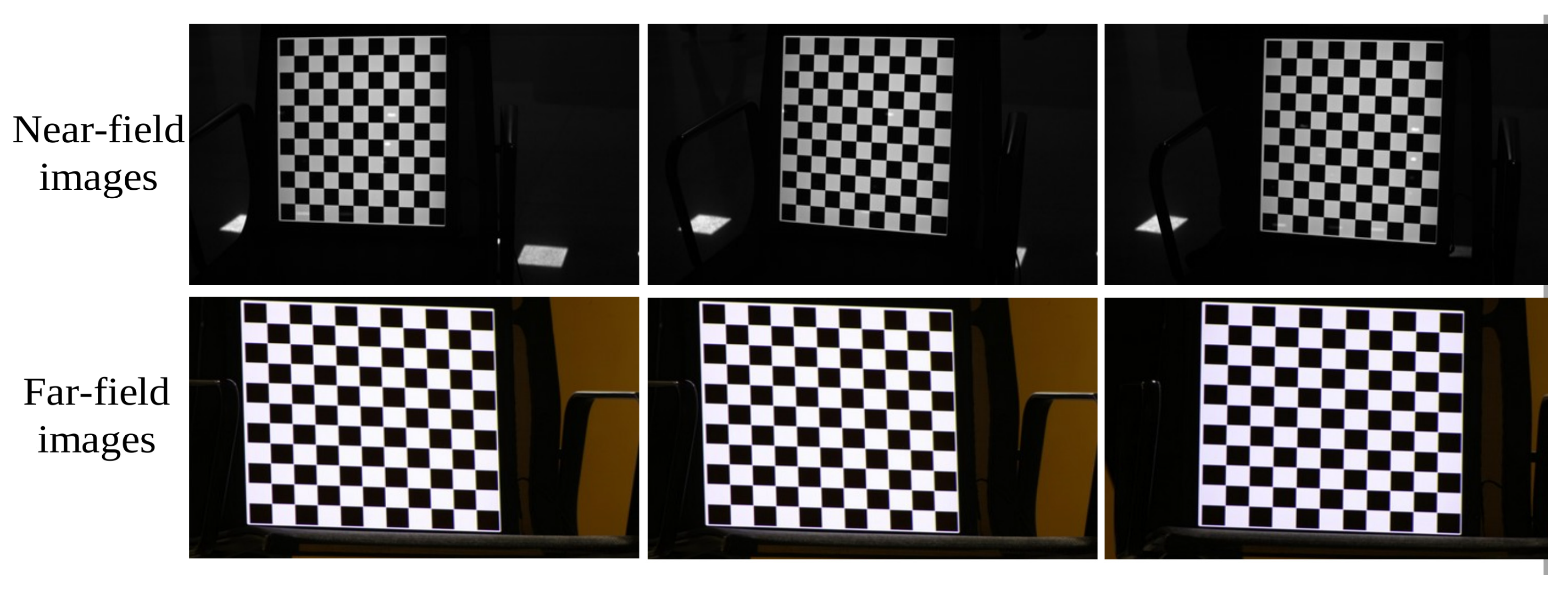
3.3.2. Planar-Target Results

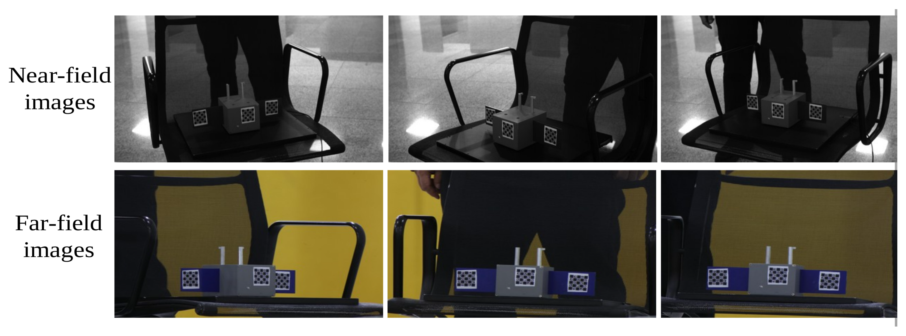
The checkerboard was placed at 40 different poses and imaged simultaneously by both cameras. Example near-field and far-field images are shown in Figure 22. Checkerboard corners were detected at subpixel precision, and their localization uncertainties were represented by empirical feature-reliability scales. Localization uncertainty was estimated from 156 near/far frames containing 8696 feature points. The median/P95 coordinate uncertainties are 0.054/0.070 pixel (checkerboard near), 2.806/6.000 pixels (checkerboard far), 0.132/0.387 pixel (aircraft near), 1.323/7.001 pixels (aircraft far), 0.173/1.294 pixel (satellite near), and 1.923/9.247 pixels (satellite far).

Table 10. Relative-pose-change disagreements for the checkerboard experiment using the near-field camera estimate as a reference.

Error	DLT	EPnP	RPnP	RPnP-LM	RPnP-CS	WCS-1C	WCS-3C	WCS-9C
$e_{\mathrm{r}\mathrm{o}\mathrm{t}}$	0.1350	0.1349	0.0930	0.0929	0.0931	0.0918	0.0926	0.0953
$e_{\mathrm{t}\mathrm{r}\mathrm{a}\mathrm{n}}$	850.6907	235.9967	67.7046	67.4541	67.0505	64.7549	65.9849	64.3823

$e_{\mathrm{r}\mathrm{o}\mathrm{t}}$ denotes the Frobenius-norm rotation error; $e_{\mathrm{t}\mathrm{r}\mathrm{a}\mathrm{n}}$ denotes the Euclidean translation error in millimeters.

summarizes the robust-RMS relative-pose disagreements for the checkerboard. DLT and EPnP exhibit large translation disagreements under the long-focal-length geometry. The best weighted configuration reduces the RPnP translation disagreement from 67.7046 to 64.3823, a reduction of approximately 4.9%. Rotation disagreements remain close among the RPnP-based variants. The translation benefit is modest under this comparison protocol.

3.3.3. Aircraft-Model Results

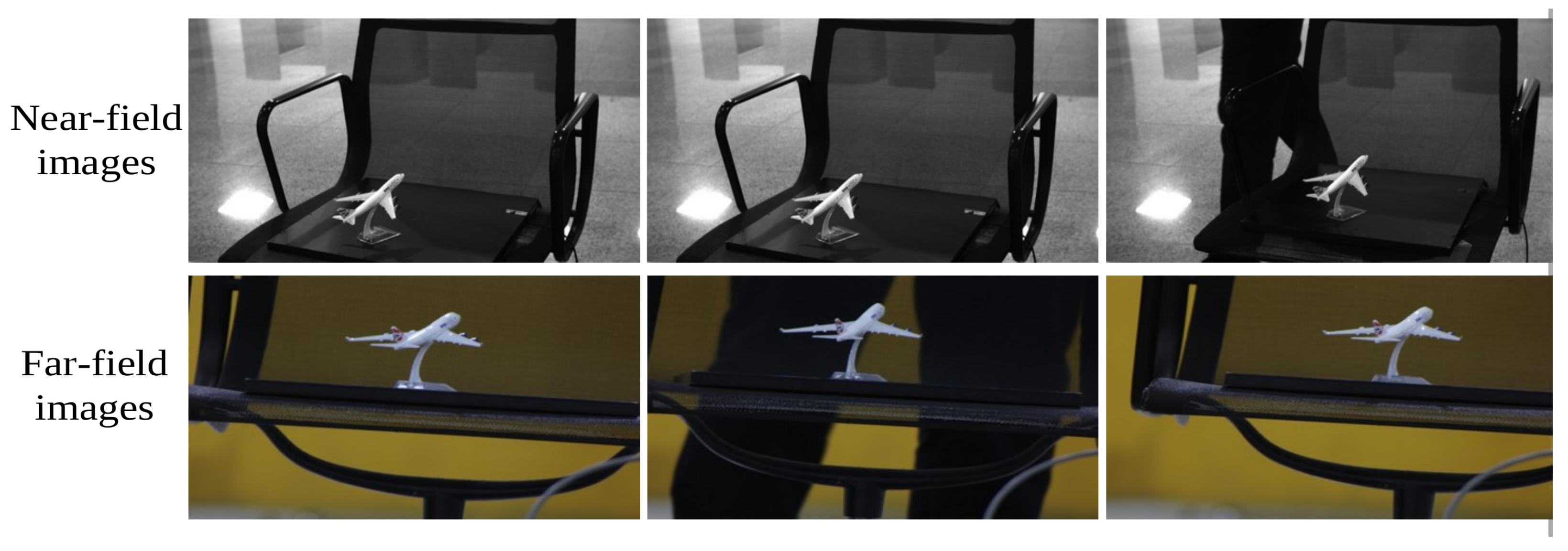
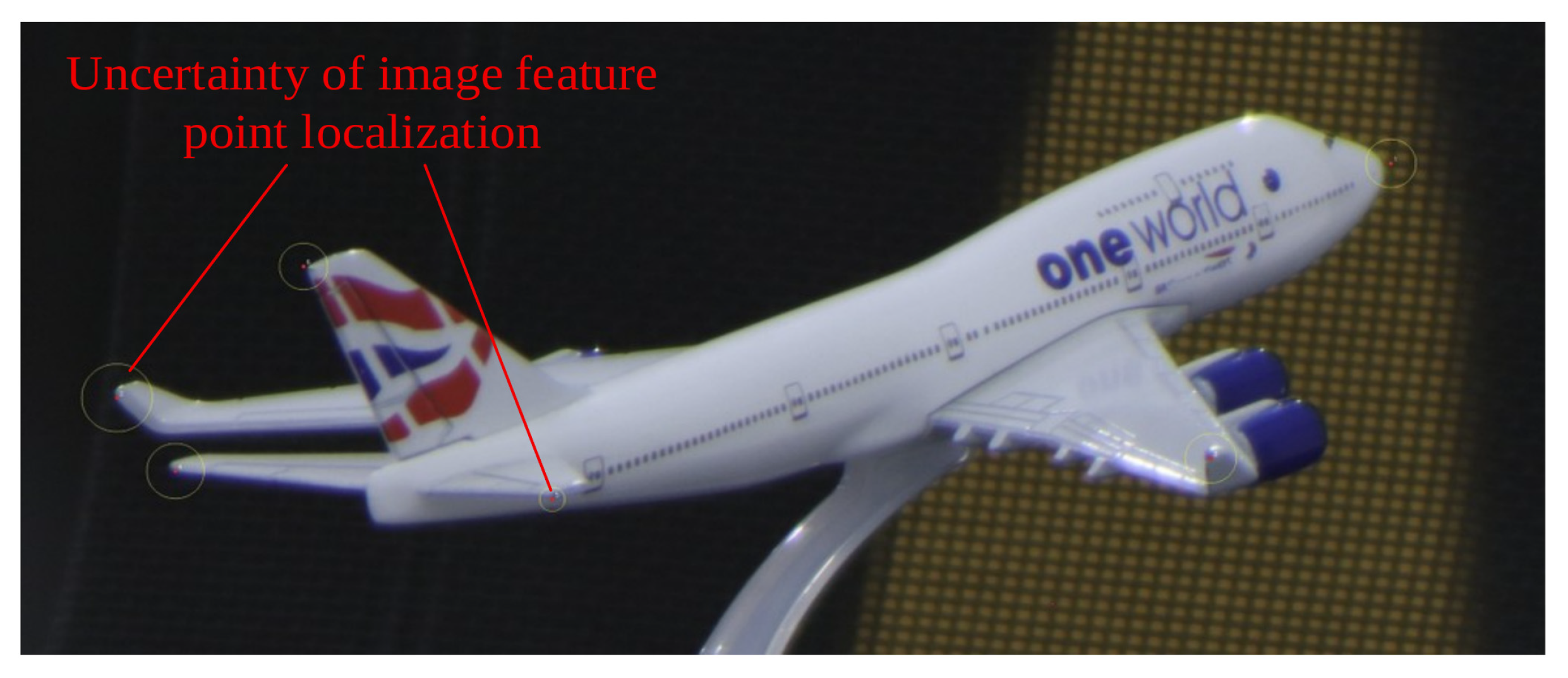
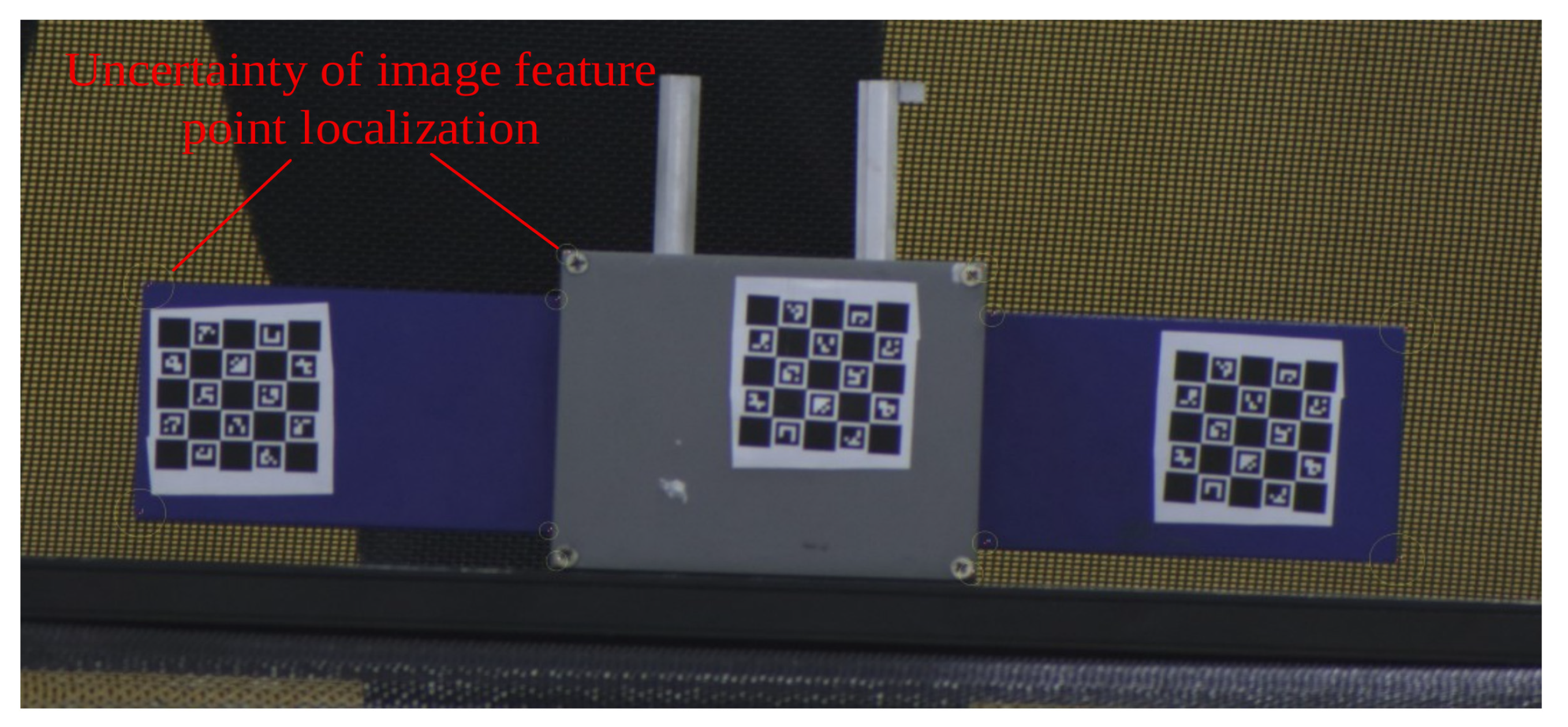
The aircraft model was placed at 18 poses. Figure 23 shows representative near-field and far-field images, and Figure 24 shows six extracted feature points with their estimated localization-uncertainty radii.

As shown in

Table 11. Relative-pose-change disagreements for the aircraft-model experiment using the near-field camera estimate as a reference.

Error	DLT	EPnP	RPnP	RPnP-LM	RPnP-CS	WCS-1C	WCS-3C	WCS-9C
$e_{\mathrm{r}\mathrm{o}\mathrm{t}}$	2.0957	1.8772	0.1189	0.1193	0.1193	0.1193	0.1193	0.1193
$e_{\mathrm{t}\mathrm{r}\mathrm{a}\mathrm{n}}$	161.2104	6.3157 × 103	286.0094	276.7685	276.7644	276.7653	276.7664	276.7691

The small difference between the nonlinear RPnP variants is small in this sample.

, RPnP-CS reduces the translation disagreement from 286.0094 for RPnP to 276.7644, a reduction of approximately 3.2%. The weighted variants give similar results. The small image footprint and limited feature-localization precision restrict the improvement in this six-point configuration. The EPnP translation value of $6.3157\times 10^3$ corresponds to solver divergence.

3.3.4. Satellite-Model Results

The satellite model was placed at 20 poses. Representative images and feature-localization uncertainties are shown in Figure 25 and Figure 26, respectively.

Table 12. Relative-pose-change disagreements for the satellite-model experiment using the near-field camera estimate as a reference.

Error	DLT	EPnP	RPnP	RPnP-LM	RPnP-CS	WCS-1C	WCS-3C	WCS-9C
$e_{\mathrm{r}\mathrm{o}\mathrm{t}}$	0.8930	2.4238	0.3254	0.2568	0.2585	0.2655	0.2586	0.2631
$e_{\mathrm{t}\mathrm{r}\mathrm{a}\mathrm{n}}$	760.9986	5.4649 × 103	631.5805	439.8077	353.1425	358.6333	360.8371	367.3882

The centrally normalized unweighted solution (RPnP-CS) produced the lowest translation error in this experiment.

shows that RPnP-LM reduces the translation disagreement by approximately 30.4% relative to RPnP, while RPnP-CS gives a reduction of approximately 44.1%. The uncertainty-weighted variants are slightly less accurate than CS in this sample. The combined centering-and-scaling stage gives the larger descriptive improvement in this dataset, while the weighting performance depends on the accuracy of the feature uncertainty model.

3.3.5. Reference Uncertainty and Common-Frame Comparison

The near-field camera provides convenient, rapid and low-cost reference measurements at a shorter working distance. Its pose estimates are used as approximate ground truth for the relative-pose comparison under the assumption that their errors are small compared with the far-field errors. Physical translations are expressed in millimeters; the approximate 1:1000 geometric analogy does not multiply the recorded errors. For an object-to-camera pose $T_{c,i}$, the relative transform $T_{c,i}^{-1}{T}_{c,j}$ cancels the fixed camera extrinsic transform, giving $R_{ij}=R_{c,i}^T{R}_{c,j}$ and $t_{ij}=R_{c,i}^T(t_{c,j}-t_{c,i})$ in the object frame at placement i.

Table 10, Table 11 and Table 12 summarize the original native-camera component differences. The common-object-frame comparison uses the same saved poses and corresponding placements.

Table 13. Physical reference observations and median per-frame RPnP reprojection RMS.

Target	Placements	Pairs per Method	Near RMS (px)	Far RMS (px)
Checkerboard	40	780	0.6393	1.1023
Aircraft	18	153	1.8620	10.4829
Satellite	20	190	11.9239	94.8192

gives the number of placements and pairs and the near/far reference-image residuals. Pairs sharing a placement are dependent; the summaries describe this set of placements.

For translation vectors or vectorized rotation matrices in the common frame, let ${\epsilon }_F$ and ${\epsilon }_N$ denote the far-field and near-field estimation errors relative to the same pose quantity. Their observed difference is $d={\epsilon }_F-{\epsilon }_N$. With RMS evaluated over the same set of matched pairs, the triangle inequality gives

$$\left|\mathrm{R}\mathrm{M}\mathrm{S}\left(d\right)-\mathrm{R}\mathrm{M}\mathrm{S}\left({\epsilon }_F\right)\right|\le \mathrm{R}\mathrm{M}\mathrm{S}\left({\epsilon }_N\right)$$

(45)

When $\mathrm{R}\mathrm{M}\mathrm{S}\left({\epsilon }_N\right)\ll \mathrm{R}\mathrm{M}\mathrm{S}\left({\epsilon }_F\right)$, the near-field pose can therefore be treated as approximate ground truth at the far-field error scale. Table 13 provides an image-space check: the near-field reprojection RMS is lower for each target. This supports the reference choice, while the pose-level approximation remains the stated assumption. The same near-field estimates and paired placements are used for every method.

3.3.6. Unfiltered Relative-Pose Comparisons

Table 14. Checkerboard common-object-frame relative-pose errors (780 pairs per method).

Method	Rotation F	Rotation U	nR	Translation F (mm)	Translation U (mm)	nt
DLT	0.1127	0.1143	5	848.1971	1604.3368	155
EPnP	0.1123	0.1138	5	212.0234	217.8174	6
RPnP	0.0391	0.1413	47	14.4058	28.5612	41
LM	0.0394	0.1419	47	13.4902	26.9447	46
CS	0.0397	0.1409	47	13.0161	28.1046	48
WCS-1C	0.0391	0.0408	11	13.3501	13.9959	13
WCS-3C	0.0409	0.0424	9	15.2154	15.9011	11
WCS-9C	0.0438	0.1634	44	14.6767	15.9764	22

,

Table 15. Aircraft common-object-frame relative-pose errors (153 pairs per method).

Method	Rotation F	Rotation U	nR	Translation F (mm)	Translation U (mm)	nt
DLT	2.0689	2.0689	0	160.8029	240.2819	16
EPnP	1.8974	1.8974	0	6300.1892	6754.2943	4
RPnP	0.0360	0.0639	17	276.7488	968.2244	17
LM	0.0358	0.0595	17	267.8284	894.1211	17
CS	0.0358	0.0595	17	267.8254	894.7244	17
WCS-1C	0.0358	0.0595	17	267.8264	894.6956	17
WCS-3C	0.0358	0.0595	17	267.8270	894.6177	17
WCS-9C	0.0358	0.0595	17	267.8304	894.6182	17

and

Table 16. Satellite common-object-frame relative-pose errors (190 pairs per method).

Method	Rotation F	Rotation U	nR	Translation F (mm)	Translation U (mm)	nt
DLT	1.2908	1.2908	0	807.8725	807.8725	0
EPnP	2.4878	2.2284	38	5618.1797	5618.1797	0
RPnP	0.2304	0.3386	27	626.3973	1509.0365	38
LM	0.1805	0.2261	12	418.3941	584.3829	16
CS	0.1794	0.2271	13	335.2526	550.1338	19
WCS-1C	0.1777	0.2277	14	342.8834	551.6853	18
WCS-3C	0.1825	0.2276	12	342.6958	554.4909	19
WCS-9C	0.1826	0.2278	12	335.3368	556.4348	21

give the common-object-frame comparisons. F and U denote filtered and unfiltered RMS; n_R and n_t are the actual exclusion counts. Rotation error is the dimensionless Frobenius norm, and translation error is in mm. Each metric uses the rule in Section 3.2.5. All listed pairs are finite; this measures pose-pair completeness, separately from the optimizer convergence criteria used in the simulations.

The common-frame CS translation RMS decreases by approximately 9.6466%, 3.2244% and 46.4792% relative to RPnP for the checkerboard, aircraft and satellite, respectively. The checkerboard benefit is modest, aircraft nonlinear refinements are nearly identical, and the satellite gives the larger translation improvement. The filtered and unfiltered values also show how large pairwise disagreements affect each summary. Central normalization and uncertainty weighting are evaluated here through relative-pose agreement; interpretation across targets accounts for their different image residuals and the shared near-field reference.

4. Discussion

The simulations identify column-scale imbalance and weak depth sensitivity as the main numerical difficulties in far-field pose refinement. Scaling supplies most of the median component-ablation improvement, centering changes the residual-space common mode, and damping stabilizes the update. The weak-mode analysis shows how these operations affect solution dispersion. Across the three turbulence strengths, CS maintains a translation improvement, while a full covariance model improves rotation estimation by representing the spatial correlation of the measurement disturbance.

The weakest physical mode is dominated by depth translation for both LM and CS. In the planar trials, CS reduces the upper tail of solution drift along this mode; the three-dimensional trials show smaller changes. This behavior is consistent with the information-matrix decomposition in Section 2.4: normalization balances the working system, while the weak pose directions remain governed by the observation geometry.

The uncertainty-sensitivity tests show that preserving the feature-to-uncertainty correspondence is more consequential than changing a global precision scale. The checkerboard benefits modestly from weighting, whereas the aircraft and satellite comparisons show similar or slightly larger errors for WCS than for CS. These comparisons evaluate uncertainty weighting through empirical relative feature reliability. An absolute uncertainty calibration serves the additional purpose of assigning coverage to pose intervals, while CS supplies the corresponding unweighted refinement.

The preprocessing acts on the local Jacobian and is compatible with residuals formed from points, lines, contours, skeletons, or surface normals. Its computational cost reflects the additional matrix construction and refinement stages. Vectorized Jacobian evaluation and parallel weight construction are possible routes to reducing this cost for applications with demanding update rates.

The physical experiments quantify relative-pose-change agreement using the near-field camera as approximate ground truth under the small-reference-error assumption in Section 3.3.5. This convenient, low-cost arrangement supports comparisons at the far-field error scale. The atmospheric model evaluates short-exposure spatial feature displacement under prescribed optical and turbulence parameters. Operational absolute accuracy and exposure-dependent image degradation require a broader measurement and calibration study.

5. Conclusions

This paper presents a far-field PnP refinement method based on weighted central normalization. RPnP initializes the pose, centering and column scaling balance the Jacobian, and uncertainty weighting incorporates feature reliability. At a 10,000 mm focal length with 1-pixel noise and moderate atmospheric turbulence, CS reduces robust-RMS rotation and translation errors by 53.2% and 21.0% relative to RPnP. Representing the full spatial covariance reduces mean rotation error by 59.3% relative to a diagonal model. The component ablation identifies the roles of scaling, centering, weighting, and damping, and the scaled physical experiments demonstrate improved relative-pose agreement. These results support central normalization for far-field pose refinement and covariance weighting when a suitable uncertainty model is available. The physical results assess relative-pose agreement using the near-field camera as approximate ground truth under the small-reference-error assumption.

References

1. Fan, R.; Xu, T.-B.; Wei, Z. Estimating 6D Aircraft Pose from Keypoints and Structures. Remote Sens. 2021, 13, 663. [Google Scholar] [CrossRef] [Scilit]
2. Li, J.; Zhuang, Y.; Peng, Q.; Zhao, L. Pose Estimation of Non-Cooperative Space Targets Based on Cross-Source Point Cloud Fusion. Remote Sens. 2021, 13, 4239. [Google Scholar] [CrossRef] [Scilit]
3. Opromolla, R.; Vela, C.; Nocerino, A.; Lombardi, C. Monocular-Based Pose Estimation Based on Fiducial Markers for Space Robotic Capture Operations in GEO. Remote Sens. 2022, 14, 4483. [Google Scholar] [CrossRef] [Scilit]
4. Opromolla, R.; Fasano, G.; Rufino, G.; Grassi, M. A Review of Cooperative and Uncooperative Spacecraft Pose Determination Techniques for Close-Proximity Operations. Prog. Aerosp. Sci. 2017, 93, 53–72. [Google Scholar] [CrossRef] [Scilit]
5. Pasqualetto Cassinis, L.; Fonod, R.; Gill, E. Review of the Robustness and Applicability of Monocular Pose Estimation Systems for Relative Navigation with an Uncooperative Spacecraft. Prog. Aerosp. Sci. 2019, 110, 100548. [Google Scholar] [CrossRef] [Scilit]
6. Kelsey, J.M.; Byrne, J.; Cosgrove, M.; Seereeram, S.; Mehra, R.K. Vision-Based Relative Pose Estimation for Autonomous Rendezvous and Docking. In Proceedings of the 2006 IEEE Aerospace Conference, Big Sky, MT, USA, 4–11 March 2006; pp. 1–20. [Google Scholar] [CrossRef] [Scilit]
7. Bourdis, N.; Marraud, D.; Sahbi, H. Camera Pose Estimation Using Visual Servoing for Aerial Video Change Detection. In Proceedings of the 2012 IEEE International Geoscience and Remote Sensing Symposium, Munich, Germany, 22–27 July 2012; pp. 3459–3462. [Google Scholar] [CrossRef] [Scilit]
8. Khan, S.A.; Ali, A.; Shiyou, Y.; Tong, J. Reconfigurable Asymmetric Embedded Magnetorquers for Attitude Control of Nanosatellites. IEEE J. Miniaturization Air Space Syst. 2021, 2, 236–243. [Google Scholar] [CrossRef] [Scilit]
9. Haralick, R.M.; Lee, C.-N.; Ottenberg, K.; Nölle, M. Review and Analysis of Solutions of the Three Point Perspective Pose Estimation Problem. Int. J. Comput. Vis. 1994, 13, 331–356. [Google Scholar] [CrossRef] [Scilit]
10. Abdel-Aziz, Y.I.; Karara, H.M. Direct Linear Transformation from Comparator Coordinates into Object Space Coordinates in Close-Range Photogrammetry. Photogramm. Eng. Remote Sens. 2015, 81, 103–107. [Google Scholar] [CrossRef] [Scilit]
11. Gao, X.-S.; Hou, X.-R.; Tang, J.; Cheng, H.-F. Complete Solution Classification for the Perspective-Three-Point Problem. IEEE Trans. Pattern Anal. Mach. Intell. 2003, 25, 930–943. [Google Scholar] [CrossRef] [Scilit]
12. Kneip, L.; Scaramuzza, D.; Siegwart, R. A Novel Parametrization of the Perspective-Three-Point Problem for a Direct Computation of Absolute Camera Position and Orientation. In Proceedings of the 2011 IEEE Conference on Computer Vision and Pattern Recognition, Colorado Springs, CO, USA, 20–25 June 2011; pp. 2969–2976. [Google Scholar] [CrossRef] [Scilit]
13. Lepetit, V.; Moreno-Noguer, F.; Fua, P. EPnP: An Accurate O(n) Solution to the PnP Problem. Int. J. Comput. Vis. 2009, 81, 155–166. [Google Scholar] [CrossRef] [Scilit]
14. Hesch, J.A.; Roumeliotis, S.I. A Direct Least-Squares (DLS) Method for PnP. In Proceedings of the 2011 IEEE International Conference on Computer Vision, Barcelona, Spain, 6–13 November 2011; pp. 383–390. [Google Scholar] [CrossRef] [Scilit]
15. Kneip, L.; Li, H.; Seo, Y. UPnP: An Optimal O(n) Solution to the Absolute Pose Problem with Universal Applicability. In Computer Vision—ECCV 2014; Springer: Cham, Switzerland, 2014; pp. 127–142. [Google Scholar] [CrossRef] [Scilit]
16. Terzakis, G.; Lourakis, M. A Consistently Fast and Globally Optimal Solution to the Perspective-n-Point Problem. In Computer Vision—ECCV 2020; Springer: Cham, Switzerland, 2020; pp. 478–494. [Google Scholar] [CrossRef] [Scilit]
17. DeMenthon, D.F.; Davis, L.S. Model-Based Object Pose in 25 Lines of Code. Int. J. Comput. Vis. 1995, 15, 123–141. [Google Scholar] [CrossRef] [Scilit]
18. Lu, C.-P.; Hager, G.D.; Mjolsness, E. Fast and Globally Convergent Pose Estimation from Video Images. IEEE Trans. Pattern Anal. Mach. Intell. 2000, 22, 610–622. [Google Scholar] [CrossRef] [Scilit]
19. Li, S.; Xu, C.; Xie, M. A Robust O(n) Solution to the Perspective-n-Point Problem. IEEE Trans. Pattern Anal. Mach. Intell. 2012, 34, 1444–1450. [Google Scholar] [CrossRef] [Scilit]
20. Schweighofer, G.; Pinz, A. Robust Pose Estimation from a Planar Target. IEEE Trans. Pattern Anal. Mach. Intell. 2006, 28, 2024–2030. [Google Scholar] [CrossRef] [Scilit]
21. Ferraz, L.; Binefa, X.; Moreno-Noguer, F. Very Fast Solution to the PnP Problem with Algebraic Outlier Rejection. In Proceedings of the 2014 IEEE Conference on Computer Vision and Pattern Recognition, Columbus, OH, USA, 23–28 June 2014; pp. 501–508. [Google Scholar] [CrossRef] [Scilit]
22. Chen, H.; Wang, P.; Wang, F.; Tian, W.; Xiong, L.; Li, H. EPro-PnP: Generalized End-to-End Probabilistic Perspective-N-Points for Monocular Object Pose Estimation. In Proceedings of the IEEE/CVF Conference on Computer Vision and Pattern Recognition, New Orleans, LA, USA, 19–24 June 2022; pp. 2781–2790. [Google Scholar]
23. Brachmann, E.; Krull, A.; Nowozin, S.; Shotton, J.; Michel, F.; Gumhold, S.; Rother, C. DSAC—Differentiable RANSAC for Camera Localization. In Proceedings of the IEEE Conference on Computer Vision and Pattern Recognition, Honolulu, HI, USA, 21–26 July 2017; pp. 6684–6692. [Google Scholar]
24. Peng, S.; Liu, Y.; Huang, Q.; Zhou, X.; Bao, H. PVNet: Pixel-Wise Voting Network for 6DoF Pose Estimation. In Proceedings of the IEEE/CVF Conference on Computer Vision and Pattern Recognition, Long Beach, CA, USA, 15–20 June 2019; pp. 4561–4570. [Google Scholar]
25. Sharma, S.; D’Amico, S. Neural Network-Based Pose Estimation for Noncooperative Spacecraft Rendezvous. IEEE Trans. Aerosp. Electron. Syst. 2020, 56, 4638–4658. [Google Scholar] [CrossRef] [Scilit]
26. Urban, S.; Leitloff, J.; Hinz, S. MLPnP—A Real-Time Maximum Likelihood Solution to the Perspective-n-Point Problem. ISPRS Ann. Photogramm. Remote Sens. Spat. Inf. Sci. 2016, III-3, 131–138. [Google Scholar] [CrossRef] [Scilit]
27. Vakhitov, A.; Ferraz, L.; Agudo, A.; Moreno-Noguer, F. Uncertainty-Aware Camera Pose Estimation from Points and Lines. In Proceedings of the IEEE/CVF Conference on Computer Vision and Pattern Recognition, Nashville, TN, USA, 20–25 June 2021; pp. 4659–4668. [Google Scholar]
28. Kendall, A.; Cipolla, R. Modelling Uncertainty in Deep Learning for Camera Relocalization. In Proceedings of the 2016 IEEE International Conference on Robotics and Automation, Stockholm, Sweden, 16–21 May 2016; pp. 4762–4769. [Google Scholar] [CrossRef] [Scilit]
29. Triggs, B.; McLauchlan, P.F.; Hartley, R.I.; Fitzgibbon, A.W. Bundle Adjustment—A Modern Synthesis. In Vision Algorithms: Theory and Practice; Triggs, B., Zisserman, A., Szeliski, R., Eds.; Springer: Berlin/Heidelberg, Germany, 2000; pp. 298–372. [Google Scholar] [CrossRef] [Scilit]
30. Levenberg, K. A Method for the Solution of Certain Non-Linear Problems in Least Squares. Q. Appl. Math. 1944, 2, 164–168. [Google Scholar] [CrossRef] [Scilit]
31. Marquardt, D.W. An Algorithm for Least-Squares Estimation of Nonlinear Parameters. J. Soc. Ind. Appl. Math. 1963, 11, 431–441. [Google Scholar] [CrossRef] [Scilit]
32. Moré, J.J. The Levenberg–Marquardt Algorithm: Implementation and Theory. In Numerical Analysis; Watson, G.A., Ed.; Springer: Berlin/Heidelberg, Germany, 1978; pp. 105–116. [Google Scholar] [CrossRef] [Scilit]
33. Zhang, Z. A Flexible New Technique for Camera Calibration. IEEE Trans. Pattern Anal. Mach. Intell. 2000, 22, 1330–1334. [Google Scholar] [CrossRef] [Scilit]
34. Hartley, R.; Zisserman, A. Multiple View Geometry in Computer Vision, 2nd ed.; Cambridge University Press: Cambridge, UK, 2004. [Google Scholar]
35. Roddier, F. The Effects of Atmospheric Turbulence in Optical Astronomy. Prog. Opt. 1981, 19, 281–376. [Google Scholar] [CrossRef] [Scilit]
36. Maire, J.; Ziad, A.; Borgnino, J.; Martin, F. Comparison between Atmospheric Turbulence Models by Angle-of-Arrival Covariance Measurements. Mon. Not. R. Astron. Soc. 2008, 386, 1064–1068. [Google Scholar] [CrossRef] [Scilit]
Figure 1. Far-field measurement with long-focal-length optics. Dashed arrows show target sightlines, blue arrows indicate range, and red rays show projection geometry.
Aerospace 13 00846 g001
Figure 2. Overview of the proposed far-field PnP preprocessing and post-optimization framework, including RPnP-based initialization and weighted central-normalization refinement.
Aerospace 13 00846 g002
Figure 3. Perspective-projection model for a far-field object. Black arrows indicate coordinate axes and projection rays; blue arrows indicate the camera-to-object relationship and the object distance.
Aerospace 13 00846 g003
Figure 4. Information-matrix distributions under near-field and far-field simulation conditions. Grayscale shading represents the numerical matrix entries, with lighter cells indicating larger values; red numerals give the corresponding entries.
Aerospace 13 00846 g004
Figure 5. Singular-value spectra of the Jacobian matrix in near-field and far-field simulations.
Aerospace 13 00846 g005
Figure 6. Information-matrix distributions before and after central normalization. Grayscale shading represents the numerical matrix entries, with lighter cells indicating larger values; red numerals give the corresponding entries.
Aerospace 13 00846 g006
Figure 7. Singular-value spectra of the Jacobian matrix before and after central normalization.
Aerospace 13 00846 g007
Figure 8. Illustration of feature-dependent localization uncertainty. Grayscale represents image intensity, red circles mark the feature locations and uncertainty radii, and the red numerical values give the corresponding localization uncertainties.
Aerospace 13 00846 g008
Figure 9. Rotation and translation errors for planar objects at focal lengths of 100, 1000, and 10,000 mm. Each curve aggregates 100 Monte Carlo trials per image-noise level.
Aerospace 13 00846 g009
Figure 10. Rotation and translation errors for three-dimensional objects at focal lengths of 100, 1000, and 10,000 mm. Each curve aggregates 100 Monte Carlo trials per image-noise level.
Aerospace 13 00846 g010
Figure 11. Reprojection errors for planar objects at focal lengths of 100, 1000, and 10,000 mm.
Aerospace 13 00846 g011
Figure 12. Reprojection errors for three-dimensional objects at focal lengths of 100, 1000, and 10,000 mm.
Aerospace 13 00846 g012
Figure 13. Fixed-target distance, three-dimensional feature-count, and initialization sensitivity (100 paired trials per point). Curves show sequential LM, CS, and WCS refinement.
Aerospace 13 00846 g013
Figure 14. Converged-Hessian weak-mode analysis for planar and three-dimensional targets (10,000 mm focal length, 2-pixel low-SNR heteroscedastic noise; 100 paired trials). Panels (a,d): normalized algorithmic eigenvalue spectra; (b,e): median absolute loadings of the two weakest eigenvectors of H q ; (c,f): final weak-mode drift d m i n . Gray/red denote LM/CS; darker blue indicates larger loadings.
Aerospace 13 00846 g014
Figure 15. Atmospheric disturbance in a conceptual spaceborne observation geometry. (a) A satellite-mounted far-field camera observes a terrestrial target through a turbulent layer. (b) Refractive-index variations perturb the light-ray directions. (c) The resulting image displacements are spatially correlated. Blue dashed rays and open points denote nominal observations; red rays and filled points denote disturbed observations. Geometry and ray deflections are schematic.
Aerospace 13 00846 g015
Figure 16. Planar-target comparison under 1-pixel noise and turbulence (100 paired trials). DLT is rank-deficient; WCS uses oracle precision.
Aerospace 13 00846 g016
Figure 17. Method comparison for three-dimensional targets under the conditions in Figure 16. Rows correspond to focal lengths of 100, 1000, and 10,000 mm. The horizontal axis contains zero turbulence followed by r 0 = 0.20 , 0.10, and 0.05 m; smaller r 0 indicates stronger turbulence.
Aerospace 13 00846 g017
Figure 18. Controlled comparison for a three-dimensional target at a 10,000 mm focal length, 1-pixel noise, and r 0 = 0.10 m. All methods use the same 100 observations, RPnP initializations, and 1000-iteration budget. CS and WCS retain the centered and mean components. Weight + Scale is the weighted scaling baseline. Boxes show medians and interquartile ranges; whiskers extend to 1.5 interquartile ranges. Final gradient tests and actual stopping reasons are reported separately; all 500 outputs are finite, with no iteration caps.
Aerospace 13 00846 g018
Figure 19. Covariance-model and uncertainty-scale sensitivity for the same 100 trials as Figure 18. Points and bars show arithmetic means and 95% bootstrap confidence intervals. The diagonal and full models use the specified simulation parameters. Oracle WCS is included as the pointwise-precision benchmark. The two scale tests multiply all standard deviations by 0.5 and 2.
Aerospace 13 00846 g019
Figure 20. Configuration of the scaled physical experiment.
Aerospace 13 00846 g020
Figure 21. Evaluation of relative-pose-change disagreements using the near-field estimate as the reference in the transformation chain. Circled numbers 1–4 label successive target placements. Curved black arrows denote pose transformations between the camera or target frames, red arrows indicate target-frame axes, and blue double-headed arrows indicate the near-field and far-field measurement distances.
Aerospace 13 00846 g021
Figure 22. Checkerboard images captured by the near-field and far-field cameras. The top and bottom rows show near-field and far-field captures, respectively; colors belong to the acquired images and do not encode measured quantities.
Aerospace 13 00846 g022
Figure 23. Aircraft-model images captured by the near-field and far-field cameras.
Aerospace 13 00846 g023
Figure 24. Aircraft feature points and their localization uncertainties.
Aerospace 13 00846 g024
Figure 25. Satellite-model images captured by the near-field and far-field cameras.
Aerospace 13 00846 g025
Figure 26. Satellite feature points and their localization uncertainties.
Aerospace 13 00846 g026