


Abstract
Air refueling extends aircraft range and endurance, but its operational value hinges on where the refueling airspace is placed and how tanker missions are sequenced. This paper addresses the joint optimization of refueling airspace planning and tanker scheduling, in which each receiver selects a refueling point from a continuous feasible interval along a fixed route. The upper level determines refueling point locations (continuous variables), while the lower level schedules multiple heterogeneous tankers (discrete combinatorial variables); the two levels are tightly coupled through spatiotemporal constraints and fuel propagation. We propose a bottleneck-driven decoupled update (BDDU) strategy built on the Whale Optimization Algorithm (WOA). BDDU extracts bottleneck states from lower-level scheduling feedback and applies per-dimension step-size control to damp the coupling amplification effect inherent in bi-level optimization. Across three scenarios of varying coupling intensities and scales, BDDU-WOA raises the feasibility rate from 50% (WOA baseline) to 90% (+40 percentage points; , Fisher’s exact test). The gain stems from a bottleneck-aware, dimension-wise step-size control mechanism with an adaptive, parameter-free classification threshold and only two tunable parameters, adding roughly 10% computational overhead. The method is intended for pre-mission planning of large-scale air refueling operations.
1. Introduction
Air refueling realizes its operational value only when refueling airspace is placed wisely and tanker missions are sequenced efficiently. Poorly positioned airspace forces receivers to burn extra fuel on detours and holding patterns—in extreme cases, creating a paradox in which “fuel consumed en route exceeds fuel gained.” When multiple receiver batches must be serviced within narrow time windows, inadequate planning also triggers rendezvous disruptions and prolonged refueling cycles, eroding mission completion rates. Despite its importance, the joint optimization of refueling airspace location and tanker scheduling—two tightly coupled decisions—remains underexplored.
The air refueling airspace planning problem has received considerable attention. Based on how refueling airspace locations are treated, existing research falls into two categories.
Stage 1: Exogenously given refueling locations. Early studies treated refueling locations as fixed inputs, concentrating on path planning or scheduling. Sundar and Rathinam examined single-UAV routing among fixed refueling depots [1]. Kannon et al. modeled the air refueling path problem with pre-specified refueling locations on a grid [2,3]. Ferdowsi et al. restricted refueling to discrete nodes along pre-specified shortest paths, precluding continuous-interval location selection [4]. Further work addressed scheduling priority [5] and task allocation via column generation [6], but all treated refueling locations as exogenous inputs rather than decision variables.
Stage 2: Refueling locations as decision variables. More recent work began endogenizing refueling airspace locations. Toydas and Sarac were the first to treat air refueling geographic coordinates as continuous optimization variables within a MINLP framework [7], which later extended to minimize total airlift time [8]. Tan et al. addressed single-tanker single-receiver refueling airspace location under threat–fuel–time trade-offs [9]. Zhang et al. studied long-range deployment with a bi-objective model balancing fleet fuel consumption and mission timeliness [10]. Wang et al. integrated refueling point selection with task allocation, but still restricted refueling points to discrete waypoints and required exactly two refueling operations per receiver, stopping short of full endogenization in continuous space [11].
Three gaps persist: (i) continuous-interval refueling point selection—the essence of location–routing joint optimization—has not been achieved; (ii) the strong coupling between upper-level location decisions and lower-level scheduling feasibility is inadequately characterized, and no algorithm has been designed specifically for this bi-level structure; (iii) large-scale, multi-route, multi-interval collaborative scheduling under interacting rigid constraints (time windows, fuel capacity, tanker coordination) remains unaddressed.
To address these gaps, this paper makes the following contributions, compared with existing studies:
- Compared with fixed-location refueling optimization [1,2,4], in which refueling points are exogenous inputs, this paper introduces receiver refueling feasible intervals and a continuous refueling airspace location selection mechanism. A bi-level combinatorial optimization model coupling upper-level refueling airspace location configuration with lower-level multi-tanker collaborative scheduling is established, achieving location–routing joint optimization in continuous space.
- Compared with discrete location optimization [7,11], in which refueling points are confined to pre-defined waypoints or discrete candidate sets, this paper lifts that restriction, enabling full endogenization of refueling demand location. Each receiver selects its refueling point from a continuous feasible interval, bringing the formulation closer to operational reality.
- Compared with standard metaheuristics applied to bi-level problems, this paper proposes the Bottleneck-Driven Decoupled Update (BDDU) strategy, which introduces dimension-level step-size control driven by lower-level bottleneck feedback—a mechanism specifically designed to damp the coupling amplification effect that standard algorithms cannot address. BDDU extracts bottleneck states from lower-level scheduling feedback and applies per-dimension step-size control with only two added parameters and minimal computational overhead.
Recent advances in multi-agent coordination, game-theoretic mission planning, and resilient swarm control [12,13] have not yet addressed the continuous location–scheduling coupling structure that is our focus.
The remainder of the paper is organized as follows. Section 2 formally describes the problem, defines the scope and assumptions, and analyzes computational complexity. Section 3 formulates the bi-level mathematical model. Section 4 presents the BDDU-WOA algorithm. Section 5 validates the approach through computational experiments across multiple scenarios. Section 6 summarizes the findings and outlines future work.
2. Problem Description and Formulation
2.1. Scope and Assumptions
Practical air refueling missions involve many complex factors; this study necessarily abstracts from certain operational details. The research scope and modeling assumptions are defined below.
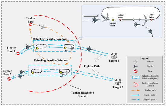
In this paper, air refueling denotes the pairing of a tanker with a receiver in a designated refueling airspace. In practice, the refueling airspace encompasses a rendezvous point, a docking point, and a separation point, whose relative spatial relationships are fixed by operational procedures. Once the rendezvous method is chosen, the docking and separation points follow directly. Hence, at the pre-planning stage, only the reference point of the refueling airspace (hereinafter the refueling point) need be determined. Figure 1 illustrates the refueling airspace geometry.
Figure 1.
Schematic of the refueling airspace geometry and its reference point.
Receivers are mission aircraft with known fuel capacity and estimated consumption rate. Each computes a “feasible refueling interval” in advance from tank capacity, mission consumption, and en-route consumption. Tankers may visit multiple refueling points per sortie provided safe return is assured, with each operation filling the receiver’s tank to capacity. All aircraft fly at constant speeds; all receivers take off synchronously. The refueling dwell time is , absorbing auxiliary docking, undocking, and formation-integration times.
The model is intended for pre-mission planning, not real-time execution, and focuses on optimizing tanker task sequences rather than flight paths.
These simplifications follow pre-mission planning conventions [7,10]. The dwell time absorbs rendezvous, docking, and separation, which are empirically stable and can be pre-calibrated. Nonlinear effects (altitude, weather, payload) pertain to real-time execution and are deferred to future work.
2.2. Bi-Level Structure: Continuous-Interval Refueling Point Location and Collaborative Tanker Scheduling
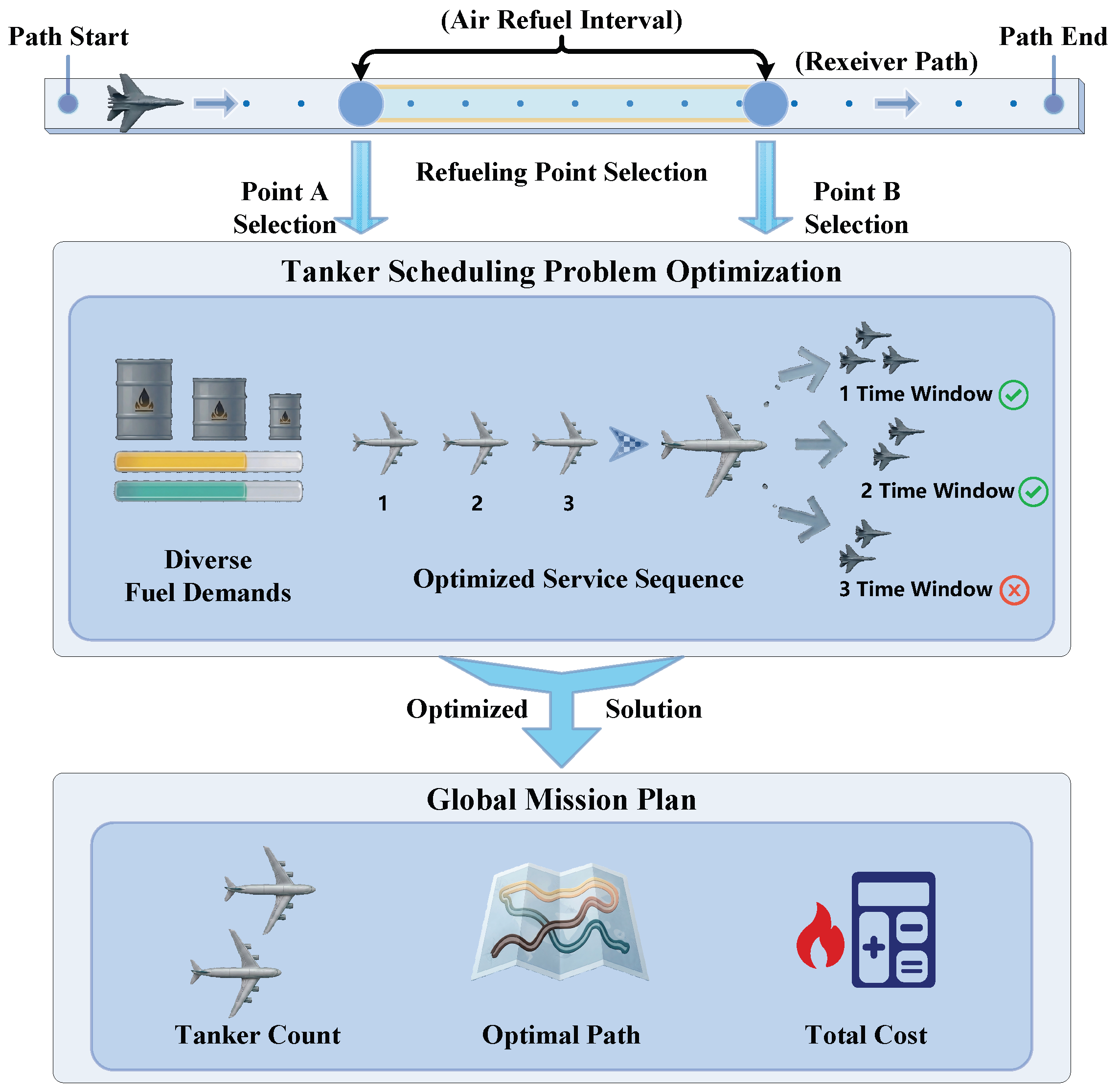
Unlike classical Vehicle Routing Problems (VRPs), where demand points are fixed known nodes, refueling demands here are distributed over selectable intervals—each corresponds to a continuous spatial range. This transforms the problem from pure routing to one with “endogenous location” decisions: both the flight path and the service sequence must be optimized, but so must the choice of refueling points within allowed intervals. The result is a bidirectional coupling between location decisions and routing. The problem naturally decomposes into two levels: the upper level determines refueling point locations (continuous variables), while the lower level handles tanker allocation and scheduling (discrete combinatorial variables).
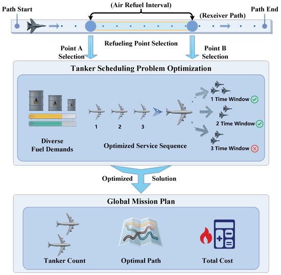
As shown in Figure 2, the upper level selects refueling point positions within each receiver’s allowed interval; the lower level then solves task allocation, service sequencing, and constraint satisfaction. Together, the two levels form a continuous–discrete hybrid space with strong coupling: small location changes at the upper level alter fuel demand and time windows at the lower level, potentially changing the number of tanker sorties, service sequences, and overall feasibility. Conversely, lower-level time window satisfaction constrains upper-level location choices.
Figure 2.
Bi-level coupled optimization structure: upper-level refueling point location configuration and lower-level multi-tanker collaborative scheduling.
Remark on “strong coupling”: Throughout this paper, “strong coupling” refers to the high sensitivity of lower-level feasibility to upper-level perturbations (Section 3.4.5), not to the intrinsic difficulty of finding feasible solutions. BDDU’s 90% feasibility on the mountain corridor vs. WOA’s 50% demonstrates algorithmic success, not weak constraints.
This problem embeds multiple rigid constraints: time windows, fuel capacity, range limits, tanker coordination, and joint determination of each demand point’s assignment and timing. Conventional metaheuristics relying solely on penalty functions produce many infeasible solutions, expending effort on feasibility repair rather than objective-driven search.
3. Bi-Level Mathematical Model
3.1. Problem Element Definitions
Receiver Flight Routes. Receivers execute missions along K predetermined routes . Route k consists of sequentially connected waypoints; the segment between waypoints n and is denoted . Routes may intersect at shared waypoints.
Refueling Points. The R refueling operations are each pre-assigned to a specific route segment. Note: Pre-assignment reflects operational practice: planners determine which segments need refueling; optimization determines precise locations within segments. Assignment–location integration is deferred to future work.
Tanker Fleet. The heterogeneous fleet of M tankers is characterized by maximum fuel capacity (kg), home base coordinates, and receiver compatibility.
Fuel Consumption. All aircraft consume fuel proportionally to distance: receiver rate (kg/km) at speed , tanker rate (kg/km) at speed . The refueling transfer rate is (kg/min). Demand at point r yields dwell time . The fuel safety threshold is .
3.2. Overall Objective
The overall objective is to minimize the number of tanker sorties, promoting efficient utilization of refueling resources in large-scale missions. In the bi-level structure, the upper-level objective F is a hierarchical composite minimizing, in order, the number of unserved refueling points, the number of tanker sorties, and total waiting time. The lower-level objective f serves solely as a greedy insertion criterion for the scheduler, selecting the best service sequence and resource allocation from among feasible alternatives to support efficient upper-level search.
3.3. Upper-Level Model: Refueling Point Location Configuration
3.3.1. Upper-Level Decision Variables
The upper-level decision variables are the refueling point location proportion vector:
where is the relative position of refueling point r along its assigned route segment. The two-dimensional geographic coordinates are obtained by path distance interpolation.
Let be the waypoint sequence of the route containing refueling point r, with total path length . The feasible interval is bracketed by the receiver’s fuel consumption profile: is where fuel drops to the threshold, triggering refueling demand, and is the farthest point before fuel reaches the safety limit . In the model, the interval width is further constrained for engineering practicality (see below). The actual refueling position follows from:
where returns the two-dimensional coordinate at distance d along the path. This parametrization normalizes each refueling point’s feasible interval to , turning the upper-level decision space into an R-dimensional hypercube amenable to metaheuristic search. The interval width is governed by the fuel safety threshold and is additionally capped for modeling tractability: . The physical interval determined by fuel consumption is ; the cap at prevents the refueling interval from covering an impractically large fraction of the route, while the 80 km lower bound ensures adequate time for docking operations.
3.3.2. Upper-Level Constraints
- (U1)
- Location proportion bounds: , . The geographic coordinates follow from path interpolation (Equation (2)), keeping refueling points within the reachable range of the receiver’s route.
- (U2)
- Indirect fuel safety constraint: Fuel safety is imposed indirectly through the interval endpoints and : places the refueling point at the fuel threshold position; places it at the latest feasible boundary. On long route segments, is small and minor changes in shift the refueling point’s time window by (Equation (17)), which can cause the tanker to miss the scheduling window even though the point remains within geographically. This design lets the bi-level coupling naturally filter feasible configurations rather than prematurely restricting the search space.
3.3.3. Upper-Level Objective Function
The upper-level objective minimizes the number of tanker sorties, with total waiting time as a secondary tiebreaker. Solution comparison follows Deb’s feasibility rules (feasible ≻ infeasible; lower score wins among feasible; lower penalty wins among infeasible), ensuring constraint violations are never traded against objective improvement.
Feasible solution scoring formula:
where
- : number of tanker sorties; is the optimal assignment returned by the lower-level scheduler (Section 3.4.1), and is the indicator function.
- : total waiting time (min), normalized by min so that waiting time acts only as a fractional tiebreaker and never outweighs a full tanker sortie.
Infeasible solution hard penalty formula:
where is the number of unserved refueling points and is the fuel infeasibility indicator function. The base value of 10,000 ensures that any infeasible solution’s penalty value far exceeds the scoring range of feasible solutions.
Remark: The hard penalty is a defensive safety boundary, not an active search driver. Its 0% trigger rate (Section 5.7) confirms BDDU’s preventive constraint handling—analogous to a safety margin that guarantees robustness without being activated.
3.4. Lower-Level Model: Collaborative Tanker Scheduling
The lower-level model takes the upper-level refueling point configuration , solves the collaborative tanker scheduling scheme, and extracts bottleneck state labels to feed back to the upper-level BDDU strategy (Section 4.3).
3.4.1. Lower-Level Decision Variables
Given the refueling point configuration output by the upper level, the following decisions are determined:
- Assignment variables: , whether refueling point r is assigned to tanker m;
- Sequencing variables: , the service sequence of tanker m, where is its assigned refueling point set;
- Time variables: , the service start time at refueling point r.
3.4.2. Lower-Level Constraints
The lower-level scheduling must satisfy the following constraints:
- (C1)
- Assignment constraint: Each refueling point is served by at most one tanker:
- (C2)
- Tanker capacity constraint: The total fuel required for tanker m—its own round-trip flight fuel consumption, the sum of fuel demands of all assigned refueling points, and the minimum safe return reserve—must not exceed its maximum fuel capacity:where is the straight-line distance from refueling point r to the tanker base, is the farthest such distance among the points assigned to tanker m (approximating the round-trip route length), is the tanker cruise fuel consumption rate, and is the minimum safe return fuel reserve. Note: This conservative bound guarantees safe return under worst-case routing. The greedy scheduler (Section 3.4.4) uses exact distances during sequence construction; the upper-level constraint serves as a rapid pre-screening filter with sufficient safety margin.
- (C3)
- Receiver fuel safety constraint: The receiver’s fuel level before receiving fuel must not drop below the safety threshold . This constraint defines the upper bound of the feasible refueling interval — is where the receiver’s fuel drops to the theoretical usable lower limit, and is the farthest position at which refueling can occur before fuel falls below . The parameter determines the exact refueling position within this interval:
- (C4)
- Time window constraint: The service start time at refueling point r must fall within its feasible time window . Given and the corresponding :where is the reference takeoff time and is the receiver cruise speed. The time window width is determined by the fuel safety threshold, so this time window is essentially the receiver fuel safety constraint expressed in scheduling terms.
- (C5)
- Service sequencing constraint: Each tanker visits its assigned refueling points in service sequence . The flight time between adjacent refueling points is the distance divided by tanker cruise speed: . The service start time must satisfy:
3.4.3. Lower-Level Objective Function
The greedy selection criterion adopted by the lower-level scheduler minimizes insertion cost:
where is the total extra time (min) introduced by the insertion, composed of three components:
Here is the time equivalent of the additional flight distance (with fixed consumption rates, ), is the extra time from insertion, and is the total waiting time. This criterion selects locally optimal insertions from the set of feasible point–tanker–position combinations. It serves only as the scheduler’s internal greedy heuristic and does not enter the global comparison of upper-level solutions.
3.4.4. Lower-Level Scheduler Design
The lower-level scheduler serves two roles: (i) evaluating each upper-level candidate (returning the number of unserved points, tanker sorties, and waiting times); and (ii) extracting bottleneck state labels (CRITICAL/TIGHT/FREE; Section 4.3.1) for the upper-level BDDU strategy. All comparison algorithms (WOA, GWO, PSO, and their BDDU variants) use this same scheduler, so performance differences stem solely from differences in upper-level search strategies.
The scheduler operates in three phases:
Phase 1—Feasibility pre-screening (). Compute time window widths for all refueling points, sort by ascending width (narrowest first), estimate the earliest serviceable time and fuel demand, and discard points that are infeasible in both time window and fuel capacity, marking them as “unserved.” The screening checks three conditions: (a) arrival within the time window (); (b) sufficient tanker fuel (); (c) adequate window width to complete refueling ().
Phase 2—Conflict resolution and sequence optimization (, with L the average number of points per tanker). Points passing pre-screening are sorted by urgency (urgency ; narrower windows and earlier deadlines receive higher priority) and processed sequentially. Each task is tested for insertion at every position in every existing tanker sequence; the best tanker and position are selected via the minimum insertion cost criterion (Equation (15)). If no existing tanker can accommodate the task, a new tanker is activated; if that also fails, the point is marked “unserved”.
Phase 3—Bottleneck label extraction (). Each refueling point is classified by its time window slackness (service completion vs. latest allowed time) into one of three states: CRITICAL (infeasible or unserved; location changes cascade to other points on intersecting routes), TIGHT (served but near the time window boundary, vulnerable to small perturbations), or FREE (ample margin, tolerant of larger search steps). Detailed definitions and the slackness computation appear in Section 4.3.1.
3.4.5. Coupling Amplification Effect
Small changes to upper-level variables can trigger disproportionate impacts on lower-level scheduling—the coupling amplification effect. To quantify this, a perturbation is applied to dimension d of :
where is the d-th standard basis vector. Define the feasibility indicator if refueling point r is served within its time window, and 1 otherwise. The coupling sensitivity of dimension d is:
counts feasibility state transitions caused by the perturbation: indicates no coupling, signals coupling. The perturbation propagates through (i) a direct effect shifting the time window of dimension d itself, and (ii) a cascading effect where feasibility changes in one refueling point cascade to downstream points on the same tanker schedule. Refueling points at intersecting routes exhibit the highest , as a single perturbation affects multiple tankers simultaneously. This heterogeneous sensitivity motivates dimension-level adaptive step-size control in BDDU.
Analytical properties of coupling sensitivity. The following properties formally characterize and establish its validity as a coupling measure. Proofs follow from the definition (Equation (18)) and the structure of the scheduling constraints (C1)–(C5).
Property 1 (Boundedness). For any and any ,
The lower bound is trivial. The upper bound follows because each of the R terms in the sum contributes at most 1 (the feasibility indicator is binary), so the total cannot exceed R.
Property 2 (Isolated-dimension insensitivity). Let d be a refueling point on a route segment that shares no waypoints with any other route. Let be the set of refueling points scheduled after d on the same tanker in the optimal schedule at . For sufficiently small (specifically, ),
The perturbation directly shifts by (Equation (17)). The direct effect can alter itself, contributing at most 1. If changes, the cascading effect propagates to at most downstream points on the same tanker. Because d lies on an isolated segment, no other tanker’s schedule is affected, so the total is bounded by .
Property 3 (Shared node amplification). Let d be a refueling point on a route segment containing a waypoint shared by multiple routes. Let be the set of routes passing through this shared node, and let be the downstream refueling points on route . Then
A perturbation at a shared node affects the scheduling of every tanker serving routes in . Each tanker may experience a cascading feasibility change along its downstream sequence. Compared with Property 2, the bound is larger by a factor proportional to , formally capturing why shared corridor nodes exhibit higher coupling sensitivity than isolated segments.
Property 4 (Localization of sensitivity). If lies in the strict interior of the feasible region—i.e., every refueling point is served with strictly positive slackness ( for all r)—then there exists a neighborhood around in which for all d. Conversely, only when at least one refueling point is at or beyond its constraint boundary. This property formalizes the intuition that coupling effects manifest only near constraint boundaries, and justifies why BDDU need only damp dimensions that are CRITICAL or TIGHT: FREE dimensions, by definition, are in the feasible interior and can safely accept full WOA steps without triggering cascading violations.
These four properties together establish as a well-defined, structurally grounded measure of per-dimension coupling intensity. Properties 2 and 3 in particular explain the empirical observation (Section 5.3.3) that on shared corridor nodes while on isolated segments. Property 4 provides the theoretical justification for the three-class bottleneck labeling scheme (Section 4.3.1): damping is only necessary where sensitivity is nonzero, and the FREE class—by construction—sits in the feasible interior.
4. Bottleneck-Driven Decoupled Update Strategy Based on Improved Whale Optimization Algorithm
This section proposes BDDU, built on WOA as the base optimizer. The core contribution is the BDDU strategy—a dimension-level step-size control mechanism generalizable to any population-based metaheuristic (GWO, PSO, etc.). Section 4.1, Section 4.2, Section 4.3, Section 4.4 and Section 4.5 present WOA basics, its bi-level limitations, the BDDU mechanism, algorithm flow, and parameter settings.
4.1. Standard Whale Optimization Algorithm
WOA [14] simulates humpback whale bubble-net foraging via three position update mechanisms: encircling prey, spiral bubble-net attack, and random search for prey. The convergence factor , which decreases linearly from 2 to 0, governs the exploration–exploitation balance. In our setting, the upper-level vector maps to the WOA search position , with .
WOA is chosen as the base optimizer for three reasons. First, its spiral mechanism and probabilistic switch between encircling and spiral update suit bi-level coupled search spaces better than GWO’s leader-following or PSO’s velocity-based momentum. Second, WOA’s direct position update (no velocity memory) simplifies per-dimension step-size control. Third, WOA references a single global best, making bottleneck state extraction straightforward. Comparative experiments (Section 5.5) confirm BDDU’s gains are not WOA-specific.
4.2. Limitations of Standard WOA in Bi-Level Coupled Problems
Direct application of standard WOA to this bi-level problem suffers from three limitations:
Limitation 1—Unified exploration–exploitation schedule. The convergence factor decreases linearly from 2 to 0 identically for all dimensions, yet constraint sensitivity is heterogeneous: shared route nodes require finer local search than isolated segments.
Limitation 2—Uniform step-size across dimensions. WOA applies the same displacement magnitude in every dimension. Large steps perturb multiple high-sensitivity dimensions at once, triggering cascading constraint violations through the coupling amplification effect and driving solutions out of the feasible region.
Limitation 3—No feasibility guidance. Standard WOA relies on a unified penalty function that ignores violation type, severity, and location. The search cannot exploit the structure of constraint violations to steer the population toward feasible regions.
These three limitations share a common cause: standard WOA is blind to the dimension-level sensitivity information that the bi-level structure provides. BDDU addresses this through bottleneck-aware per-dimension step-size control.
4.3. Bottleneck-Driven Decoupled Update Strategy
BDDU uses the spatiotemporal slackness information fed back by the lower-level scheduler to assign differentiated damping factors to each search dimension—reducing step sizes on high-sensitivity bottleneck dimensions to protect feasibility, while retaining full step sizes on low-sensitivity free dimensions to preserve exploration. “Decoupled” means each dimension follows its own independent step-size schedule dictated by its bottleneck state, rather than sharing a uniform convergence factor as in standard WOA.
BDDU forms a closed loop: upper-level configuration → lower-level scheduler evaluation → bottleneck state extraction → state label mapping → per-dimension step-size control → damped update → new . The following subsections detail each component.
4.3.1. Bottleneck State Labeling
After lower-level scheduling completes, each refueling point r (equivalently, upper-level dimension ) receives a bottleneck state label based on its time window slackness, defined as the gap between the service completion time and the latest allowed time:
Rather than using a fixed absolute threshold—which is problematic because the slackness distribution varies across problem instances and across iterations within a single run—we adopt a distribution-driven adaptive classification. At each iteration, let be the set of non-negative slackness values across all dimensions of the current best solution. The adaptive threshold is defined as the median of this set:
The state labeling function then classifies as follows:
- Critical: (service time exceeds the latest allowed time) or the refueling point is unserved. Such dimensions are infeasible and their location changes cascade through the scheduler to affect other refueling points on intersecting routes.
- Tight: . These dimensions are feasible but in the tighter half of the current population. They are served near the time window boundary, and small perturbations risk shifting them into infeasibility.
- Free: . These dimensions are in the more comfortable half of the population, with sufficient time margin to tolerate larger search steps.
This classification has three advantages over a fixed threshold. First, it is parameter-free: no parameter needs to be tuned. Second, it is self-adapting: as the search progresses and the slackness distribution shifts, tracks the distribution automatically. Third, it guarantees class occupancy: by construction, roughly half of all feasible dimensions are classified as TIGHT and half as FREE at every iteration, ensuring the three-class system remains meaningful regardless of how tight the slackness distribution becomes.
Bottleneck quality is quantified by: (i) concordance rate between predicted state and actual feasibility outcome after perturbation; (ii) intra-class homogeneity of slackness within each state; and (iii) inter-class separation between adjacent slackness distributions. The median-split design guarantees inter-class separation by construction.
4.3.2. Dimension-Level Step-Size Control
BDDU implements per-dimension step-size control by applying dimension-specific relaxation factors to the candidate positions generated by standard WOA. The candidate position is first computed by the WOA update rule, then corrected via:
where is the position proposed by the standard WOA update rule [14].
The relaxation factor is determined solely by the bottleneck state:
where . Free dimensions accept the full WOA step (), tight dimensions take a moderate fraction (), and critical dimensions take only a small fraction () to carefully navigate the infeasible region. Default values are and .
Unlike the earlier design, we deliberately omit an iteration-dependent decay schedule. The classification dynamics themselves provide a natural progression from exploration to exploitation: in early iterations, many dimensions are CRITICAL, yielding small overall steps; as constraints are resolved and dimensions migrate to TIGHT and FREE, the effective step sizes increase automatically. When most dimensions reach FREE status, BDDU approaches the full search capability of standard WOA, exploiting the feasible region without artificial restriction. If a FREE dimension later becomes CRITICAL due to an aggressive step, it is immediately reclassified and damped in the next iteration—a self-correcting mechanism.
4.4. BDDU-WOA Algorithm Flow
Algorithm 1 presents the complete BDDU-WOA procedure.
| Algorithm 1 BDDU-WOA algorithm |
|
4.5. Parameter Settings and Strategy Generalization
BDDU introduces only two free parameters, (critical step-size factor) and (tight step-size factor), with default values and . The classification threshold is computed automatically from the population slackness distribution (Equation (23)) and requires no tuning. A comprehensive sensitivity analysis of and appears in Section 5.2. BDDU is thus lightweight, adding only two tunable parameters beyond the base WOA configuration.
The BDDU mechanism is not tied to WOA. Its core logic—extracting bottleneck states from lower-level feedback and applying per-dimension adaptive step-size control—integrates readily with any population-based metaheuristic (GWO, PSO, etc.). Cross-algorithm generalization is left for future work.
5. Computational Experiments
This section evaluates the proposed BDDU-WOA algorithm on parameter sensitivity, solution quality and feasibility, component contributions (ablation), cross-scenario scalability, and computational cost.
5.1. Common Experimental Framework
The following subsections establish the hardware, metrics, and common parameters shared by all experiments. Scenario-specific settings and algorithm parameters are detailed within each experiment subsection.
5.1.1. Hardware and Software Environment
All experiments run on a single workstation (Intel Core i7-10700 @ 2.90 GHz, 16 GB RAM, MATLAB R2023b). Each trial uses a single thread to ensure wall-clock comparability.
5.1.2. Evaluation Metrics
The evaluation metrics used throughout the experimental campaign are defined in Table 1 below.
Table 1.
Evaluation metrics.
5.1.3. Common Experimental Parameters
To ensure fair comparison across all experiments, the following parameters (summarized in Table 2) are kept constant unless otherwise stated:
Table 2.
Common experimental parameters.
5.1.4. Test Scenarios
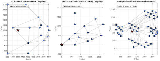
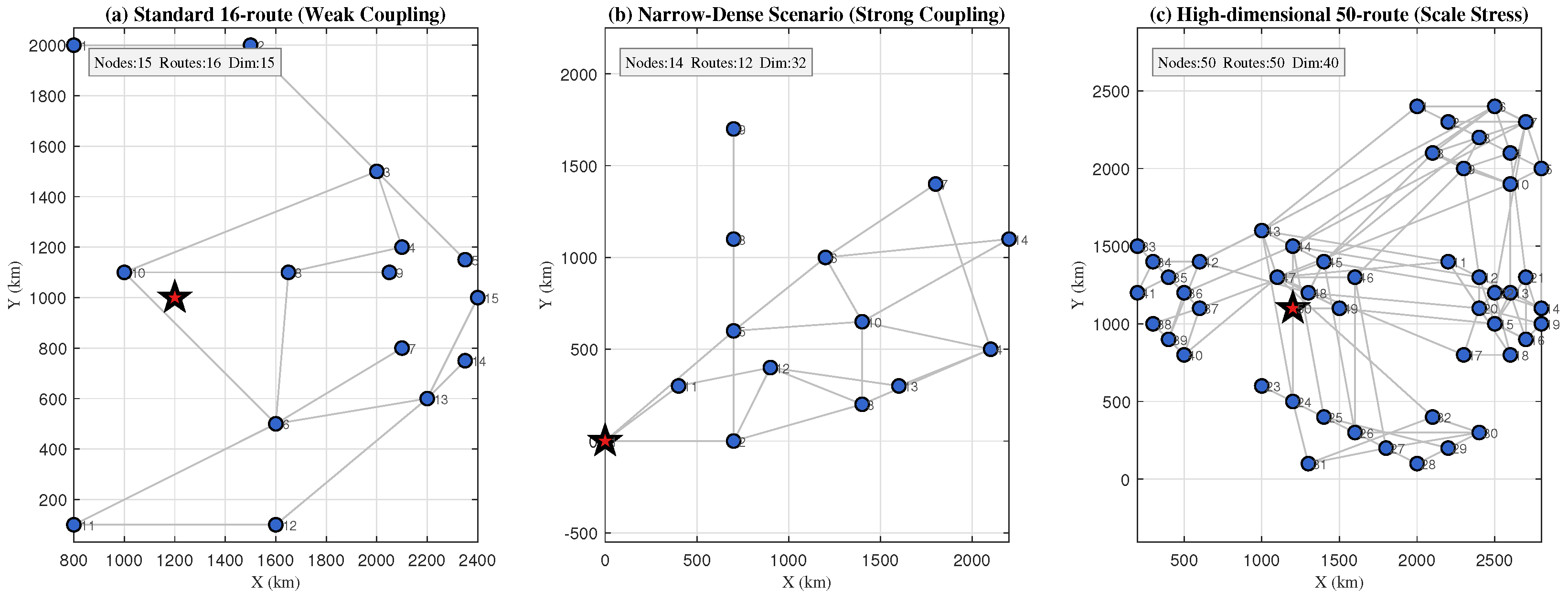
Three scenarios of varying coupling strength are used throughout the experimental campaign. Their layouts and characteristics are summarized in Figure 3 and Table 3.
Figure 3.
Three-panel scenario topology. Panel (a): Standard 16-route scenario with base station (red star) and waypoints (blue circles). Panel (b): Mountain corridor scenario with highlighted shared corridor nodes and intersecting routes. Panel (c): High-dimensional 50-route scenario showing dense route network.
Table 3.
Summary of scenario characteristics.
Scenario 1—Standard 16 routes (moderate coupling). The baseline: 15 waypoints and 16 receiver routes. Several waypoints are shared by 4–8 routes (node 6 by 8, node 10 by 6, node 11 by 6, node 8 by 5), producing moderate coupling among scheduling decisions.
Scenario 2—Mountain corridor (strong coupling). The primary test case, designed to reflect real air refueling networks in constrained airspace (mountain corridors or no-fly-zone detours): 14 waypoints, 12 receiver routes. Six core waypoints are shared by 4–8 routes (nodes 2–6 and 10). Coupling is strongest here, making this scenario the most discriminative for algorithm comparison.
Scenario 3—High-dimensional 50 routes (scalability stress test). A large-scale instance with 50 waypoints and 50 receiver routes, testing BDDU’s behavior as the number of upper-level variables and the lower-level scheduling complexity grow.
Algorithm-specific and scenario-specific settings are detailed in their respective experiments.
5.2. Experiment I: Parameter Robustness Analysis
5.2.1. Background and Motivation
To assess whether BDDU-WOA’s solution quality is sensitive to parameter settings, a comprehensive robustness analysis is conducted spanning BDDU-intrinsic parameters (, ), the adaptive classification mechanism, penalty coefficients, and algorithm control parameters. The response variables are the decomposed metrics and , analyzed via one-way ANOVA with effect size.
5.2.2. Sensitivity Analysis Design
The analysis uses Scenario 2 (32 refueling points), 20 Monte Carlo repetitions per configuration (50 iterations, population 30). To rule out ceiling effects from loose time windows, Experiment D systematically compresses window widths to 10% of original. To assess the contribution of the adaptive median-split classification, we include an ablation comparing it against a fixed threshold baseline ( min). Parameter ranges are summarized in Table 4.
Table 4.
Comprehensive parameter sensitivity analysis design.
5.2.3. Parameter Robustness Results
BDDU-Intrinsic Parameters and Diagnostics
Both BDDU parameters show no statistically significant effect on solution quality across their tested ranges (6 levels each, 20 runs/level, 100% feasibility throughout). One-way ANOVA: : , ; : , . The interaction is non-significant (). The penalty-trigger rate is below 2% across all runs; penalty weight variation (1–) produces no significant effect ().
Adaptive vs. Fixed Classification
The adaptive median-split () and the fixed threshold ( min) yield comparable solution quality, both achieving 100% feasibility. However, the adaptive classification consistently populates all three bottleneck states (CRITICAL ∼15%, TIGHT ∼43%, FREE ∼42% at convergence), whereas the fixed threshold concentrates 95%+ of points in a single class. This structural differentiation confirms that the adaptive scheme provides meaningful per-dimension differentiation without sacrificing robustness. Detailed sensitivity profiles are in Figure A1 (Appendix A).
Control Parameters and Stress Test
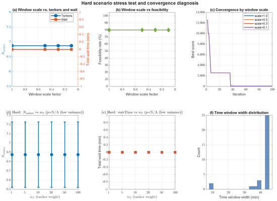
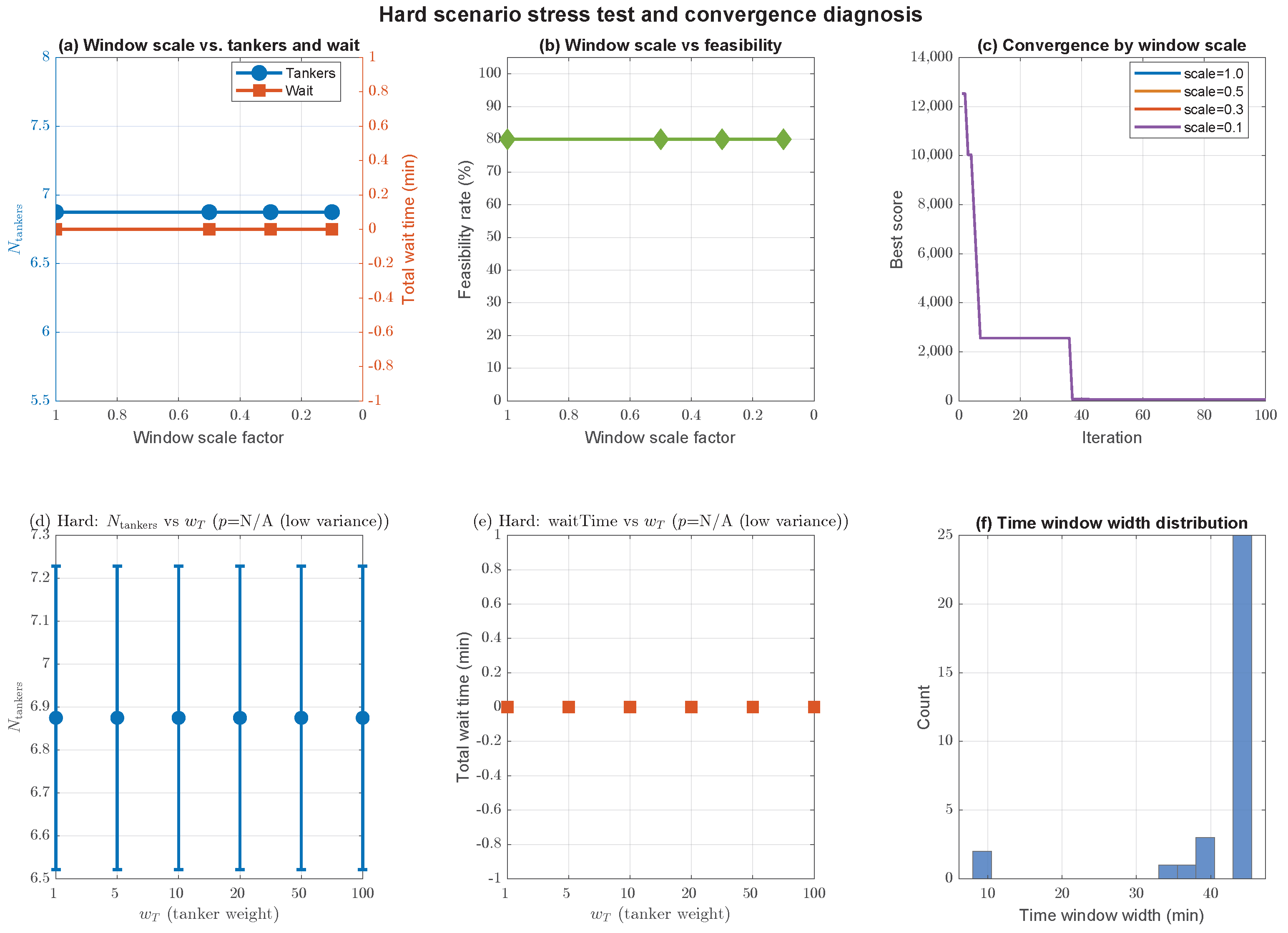
Population size (10–100), iteration budget (20–200), and initialization strategy all showed no significant effect on solution quality (all , ; Table A1 in Appendix A). Under time window compression to 10% of original width (Experiment D, Figure 4), and feasibility rate remained stable, confirming robustness is not a ceiling artifact.
Figure 4.
Hard scenario stress test. (a) and vs. window scale factor. (b) Feasibility rate remains above 90% at all scales. (c) Convergence trajectories by window scale. (d) vs. under tight windows (p = N/A, low variance). (e) Wait time vs. under tight windows (p = N/A, low variance). (f) Time window width distribution: original vs. compressed.
Practical Implications
BDDU-WOA’s near-universal parameter insensitivity means practitioners can deploy with default parameters (, ) without per-instance tuning. The median-split classification requires no threshold tuning at all. The caveat is that robustness has been demonstrated on NarrowDense benchmarks; confirmation on hub-and-spoke topologies and operational data remains future work.
5.3. Experiment II: Algorithm Comparison on the Coupling-Intensive Scenario
This experiment compares the proposed BDDU-WOA against three standard metaheuristics on the mountain corridor scenario (Scenario 2 in Section 5.1.4), which exhibits the strongest route coupling and therefore provides the most discriminative testbed for algorithmic differences.
5.3.1. Comparison Algorithms
Four algorithms are compared: three standard metaheuristic baselines and the proposed BDDU-WOA.
- Standard metaheuristics (baselines): Whale Optimization Algorithm (WOA) [14], Grey Wolf Optimizer (GWO) [15], Particle Swarm Optimization (PSO).
- Proposed method: BDDU-WOA.
The three baselines span different search paradigms (spiral exploration for WOA, leader-following hierarchy for GWO, velocity-driven momentum for PSO). BDDU-WOA integrates the bottleneck labeling mechanism and dimension-level step-size relaxation into WOA’s spiral update rules.
5.3.2. Parameter Settings
Standard parameter values from the literature are adopted. Table 5 lists the algorithm-specific parameters used in this experiment.
Table 5.
Algorithm-specific parameter settings.
5.3.3. Mountain Corridor Comparison Results
Table 6 presents the main results on the mountain corridor scenario (32 dimensions, 8500 kg fuel capacity), with 20 independent trials per algorithm. This scenario has the strongest coupling among the three test cases.
Table 6.
Performance comparison on the mountain corridor scenario (32 dimensions, 20 trials).
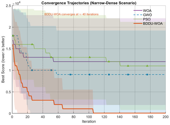
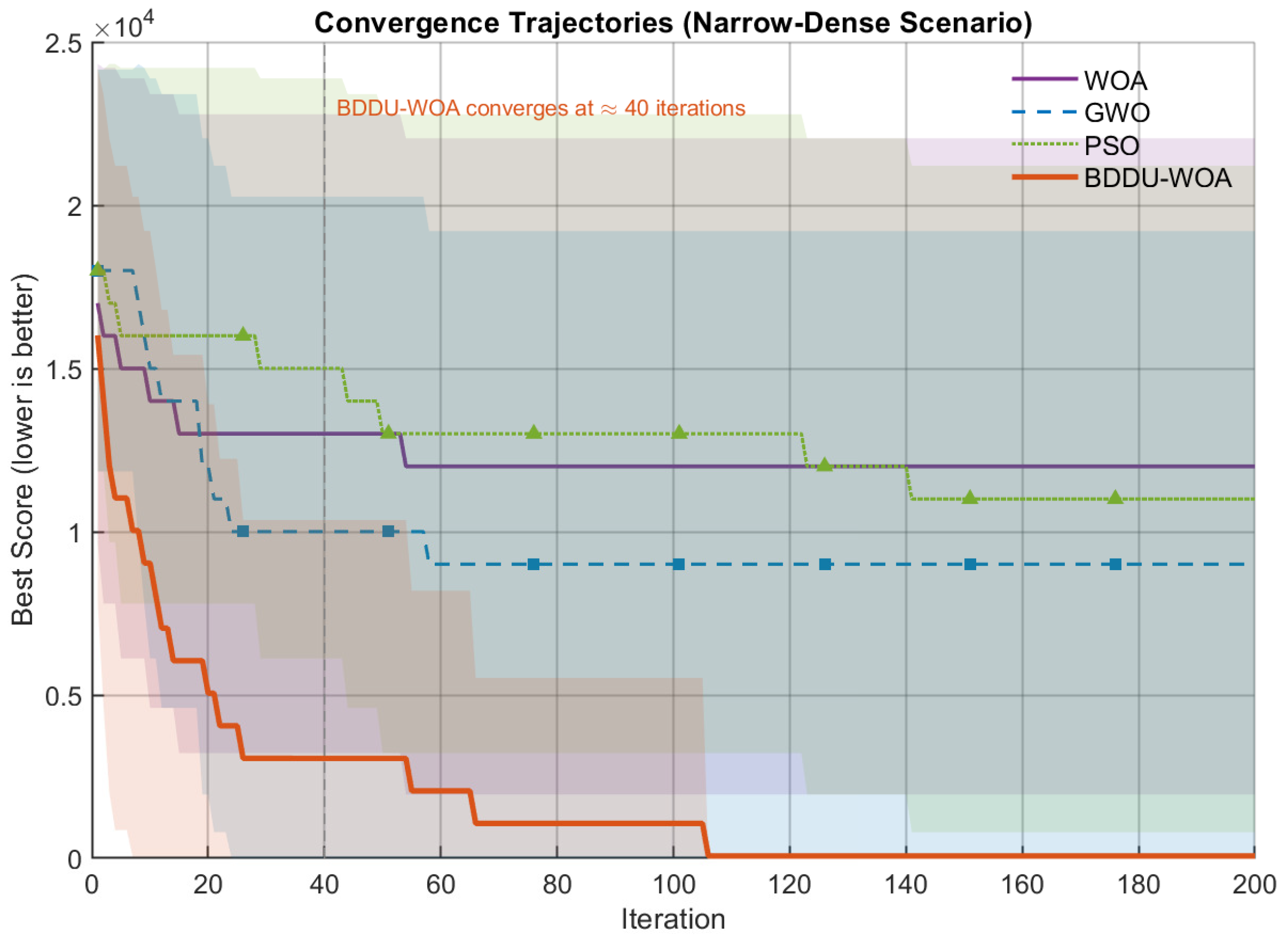
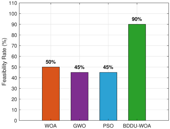
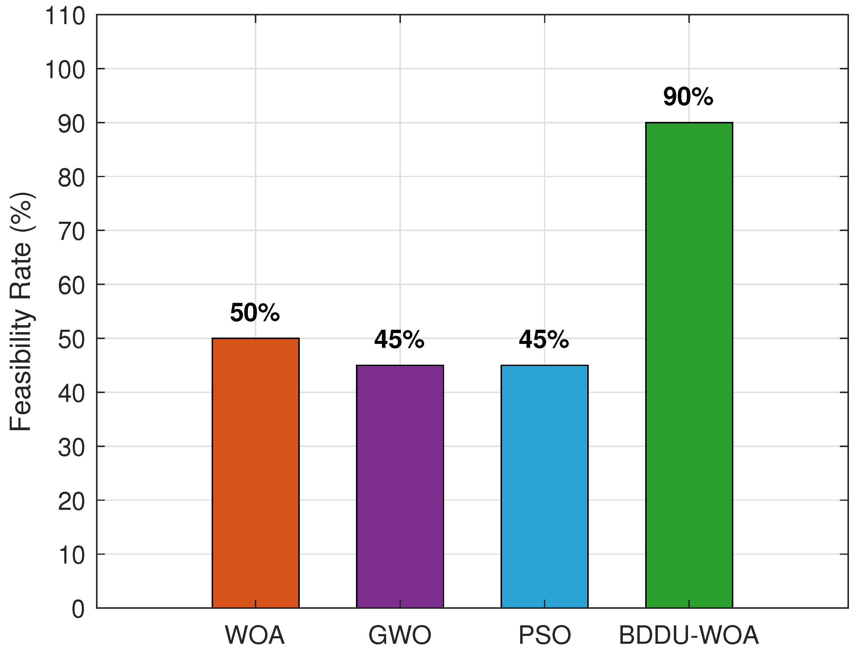
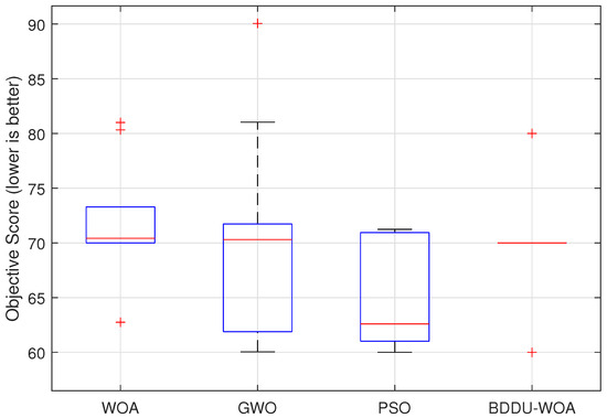
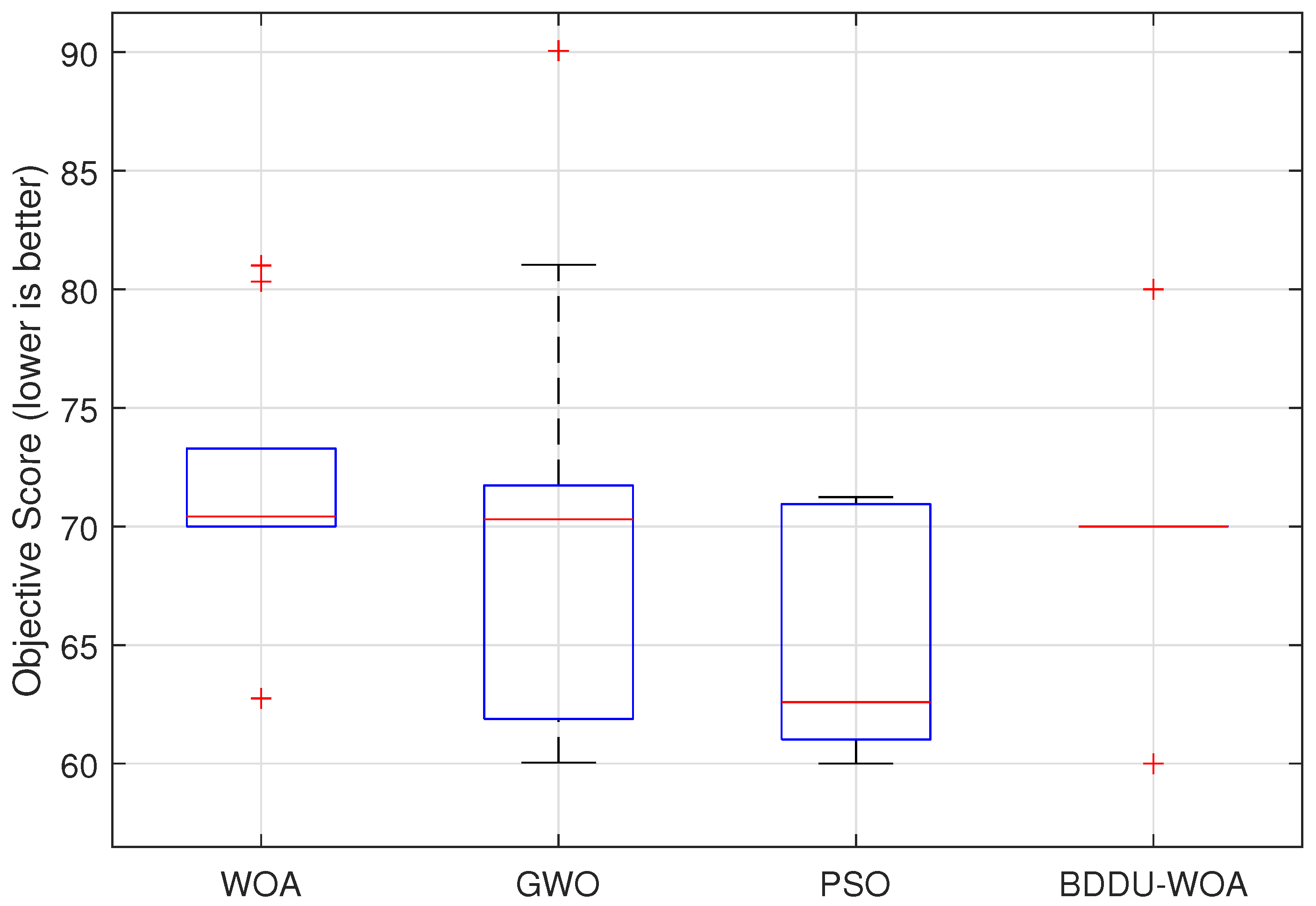
BDDU-WOA achieves 90% feasibility (18/20) vs. WOA’s 50% (10/20), a statistically significant +40 pp improvement (Fisher’s exact ). GWO and PSO both reach 45%. Among feasible runs, all four algorithms share a median tanker count of 7.0; BDDU-WOA exhibits the lowest run-to-run variability. The primary algorithmic differentiator is feasibility rate rather than optimality gap, since feasible-solution quality is largely determined by route structure and fuel constraints. The convergence behavior is shown in Figure 5, and the per-algorithm feasibility and score distributions are compared in Figure 6 and Figure 7.
Figure 5.
Convergence curves on the mountain corridor scenario (mean ± 1 SD over 20 trials). BDDU-WOA (orange, solid) converges earlier and achieves lower scores than WOA (purple, solid), GWO (blue, dashed), and PSO (green, dash-dotted). Shaded bands represent ±1 standard deviation over 20 independent trials.
Figure 6.
Feasibility rate comparison on the mountain corridor scenario (20 trials each). BDDU-WOA achieves 90%, substantially outperforming WOA (50%), GWO (45%), and PSO (45%).
Figure 7.
Score distribution of feasible solutions (20 runs each, mountain corridor). All four algorithms share a median score of 7.0. BDDU-WOA achieves the lowest run-to-run variability and its distribution reflects 90% of runs (vs. 50% for WOA).
To further substantiate the coupling amplification effect formalized in Section 3.4.5, we computed the per-dimension coupling sensitivity (Equation (18)) on the mountain corridor scenario from a baseline configuration with a perturbation of . The results show that dimensions on shared corridor nodes exhibit (up to 4 feasibility state changes per perturbation), while dimensions on isolated segments remain at . This heterogeneous sensitivity profile confirms the theoretical prediction and motivates dimension-level adaptive step-size control: high-sensitivity dimensions require smaller search steps to prevent cascading constraint violations.
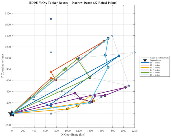
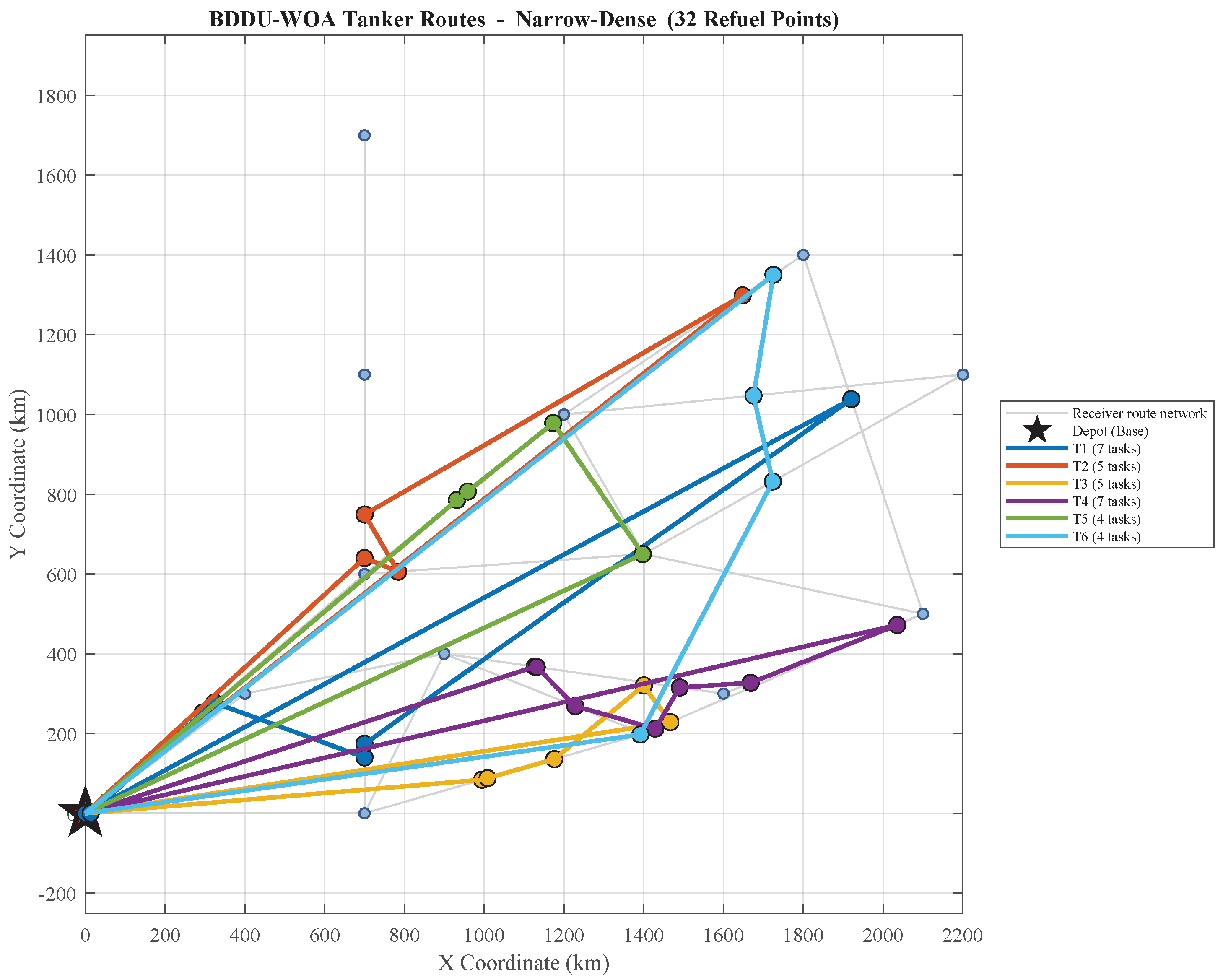
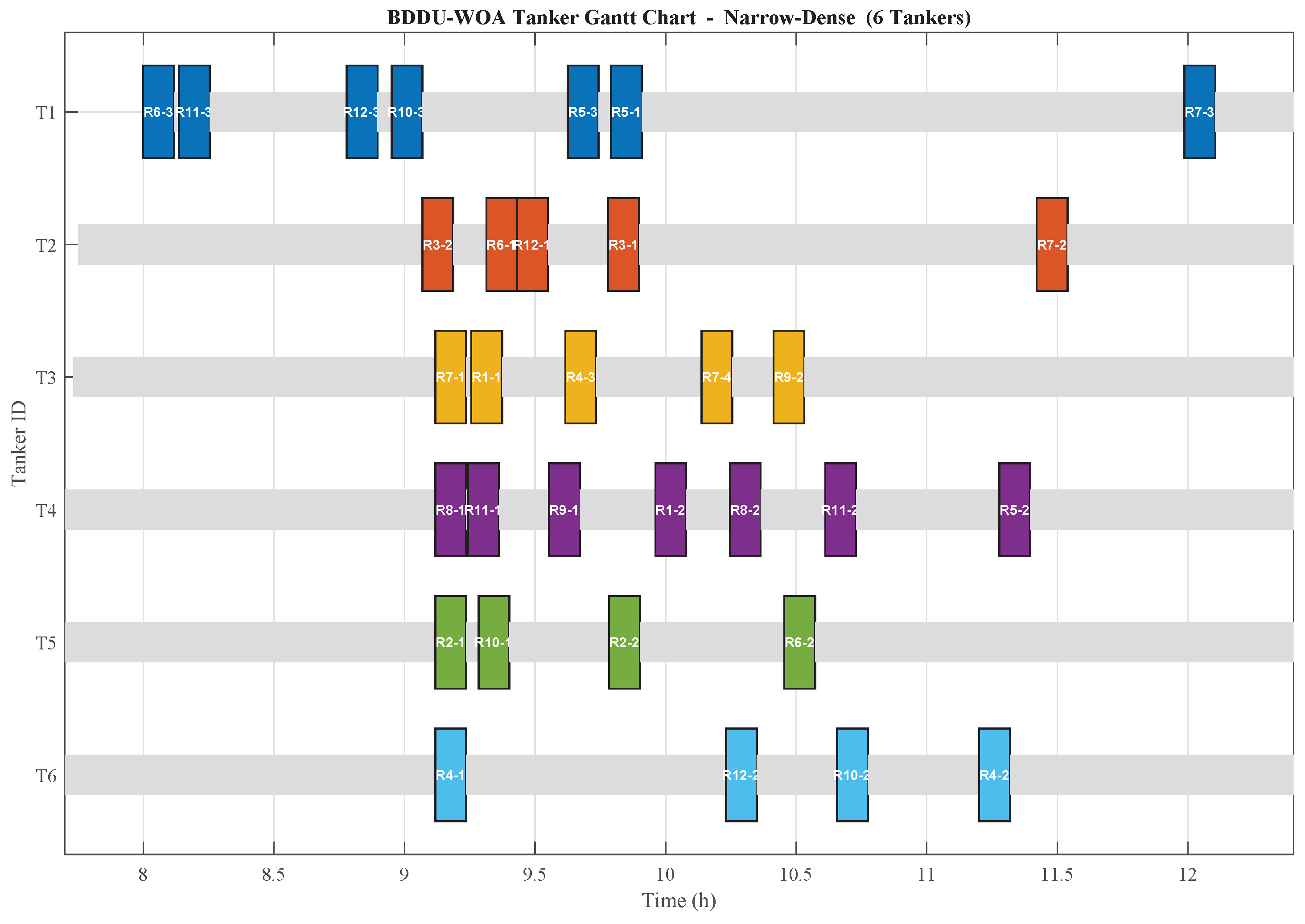
To provide a concrete view of the scheduling solutions produced by BDDU-WOA, Figure 8 overlays the tanker flight trajectories on the mountain corridor topology, and Figure 9 presents the corresponding Gantt chart.
Figure 8.
BDDU-WOA tanker routes on the mountain corridor scenario. The depot location is marked by a red star; receiver waypoints are shown as blue circles. Colored lines represent individual tanker trajectories departing from the depot, visiting assigned refueling points in sequence, and returning to base. Background gray lines show the receiver route network. Different colors distinguish different tanker IDs, and the spatial clustering of refueling points assigned to the same tanker illustrates the scheduler’s distance-minimizing insertion logic.
Figure 9.
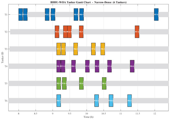
Gantt chart of the BDDU-WOA scheduling solution on the mountain corridor scenario. The horizontal axis represents mission time in minutes from takeoff; the vertical axis lists individual tanker IDs (T1–T6). Each colored bar represents a refueling service operation (color denotes tanker ID, consistent with Figure 8), with the bar length proportional to the refueling dwell time. Gray segments indicate travel time between consecutive refueling points and the return trip to base. The chart shows how refueling operations are distributed across tankers, illustrating the scheduler’s ability to pack multiple services per tanker sortie while respecting time window constraints.
5.4. Experiment III: Ablation Study
To isolate the contribution of bottleneck-driven step-size control, we compare BDDU-WOA (pure step-size control, no auxiliary mechanisms) against standard WOA under a reduced iteration budget (, 20 trials each; all other parameters are the same as in Experiment II, Table 5).
Ablation Analysis Results
BDDU-WOA lifts the feasibility rate from 30% (6/20) to 90% (18/20), a +60 percentage-point gain from a single mechanism with only two added parameters and an adaptive, parameter-free classification threshold (Table 7). At (Experiment II), BDDU-WOA reaches 90% feasibility (+40 pp over WOA’s 50%), confirming that the core mechanism delivers the dominant gain and benefits from additional iterations.
Table 7.
Ablation study (mountain corridor, , 20 trials).
5.5. Experiment IV: Cross-Scenario Scalability Validation
This experiment tests whether the advantage observed in Experiment II generalizes to moderately coupled and large-scale settings, using Scenario 1 (moderate coupling) and Scenario 3 (high-dimensional; see Table 3).
5.5.1. Cross-Scenario Test Setup
All algorithm parameters are identical to Experiment II (Table 5); only the scenario dimensionality and route topology differ.
5.5.2. Cross-Scenario Scalability Results
Standard 16-Route Scenario (Moderate Coupling)
In this moderately coupled scenario, both WOA and BDDU-WOA achieve 100% feasibility (all 20 runs feasible). BDDU-WOA reduces the mean number of tanker sorties from 7.5 to 7.0 (6.7% reduction), demonstrating that bottleneck-aware step-size control improves resource efficiency even when the baseline algorithm already finds feasible solutions (Table 8).
Table 8.
Results on the standard 16-route scenario (15 dimensions, 20 trials).
High-Dimensional 50-Route Scenario (Scalability Stress Test)
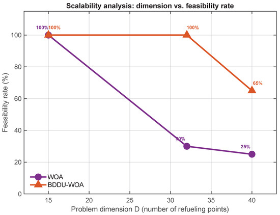
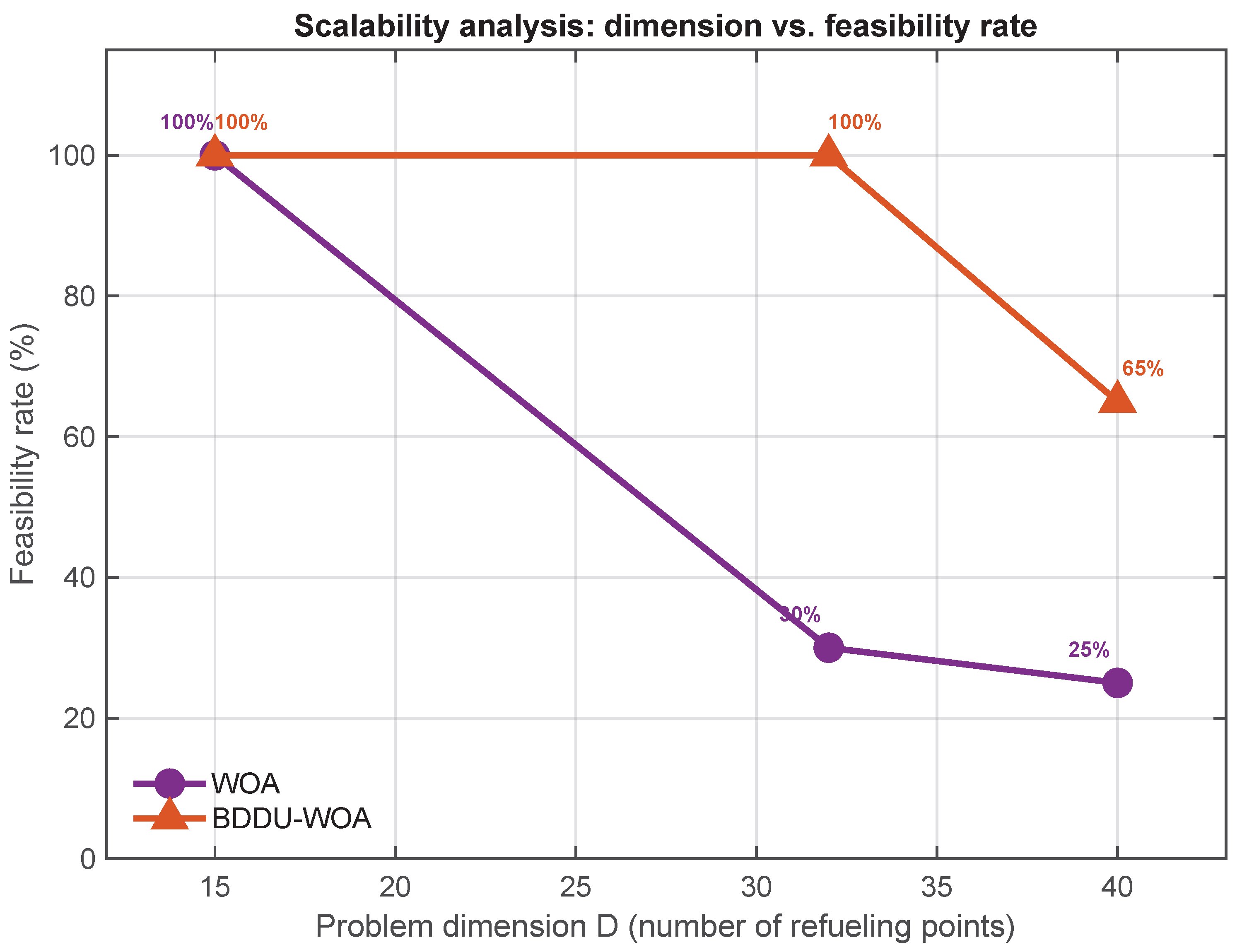
As the problem scale increases from to , standard WOA’s feasibility rate drops from 100% to 25%. BDDU-WOA maintains 65% (+40 pp over WOA at the largest scale). The widening performance gap at higher dimensions confirms that bottleneck-aware step-size control becomes increasingly valuable as the number of interacting constraints grows (Table 9). Figure 10 summarizes the feasibility rate trend across all three problem scales.
Table 9.
Results on the high-dimensional 50-route scenario (40 dimensions, 20 trials).
Figure 10.
Scalability analysis: feasibility rate as a function of problem dimension D. The horizontal axis represents the number of refueling point dimensions ( for the three test scenarios); the vertical axis shows the feasibility rate as a percentage. Two curves compare standard WOA (red, solid) and BDDU-WOA (blue, solid). BDDU-WOA maintains consistently higher feasibility rates across all dimensions, while WOA’s rate declines sharply as D increases. The widening gap confirms that BDDU’s benefit grows with problem scale and constraint coupling complexity.
5.6. Experiment V: Computational Cost Analysis
Computational Overhead Analysis
BDDU-WOA incurs approximately +10.2% overhead (3.10 s per trial; Table 10), primarily from the bottleneck label extraction after each lower-level evaluation. The cost is acceptable relative to the +40 pp feasibility gain (from 50% to 90%).
Table 10.
Computational cost comparison (mountain corridor scenario, 20 trials).
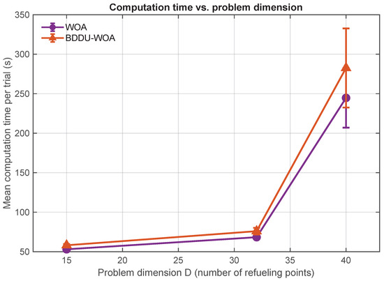
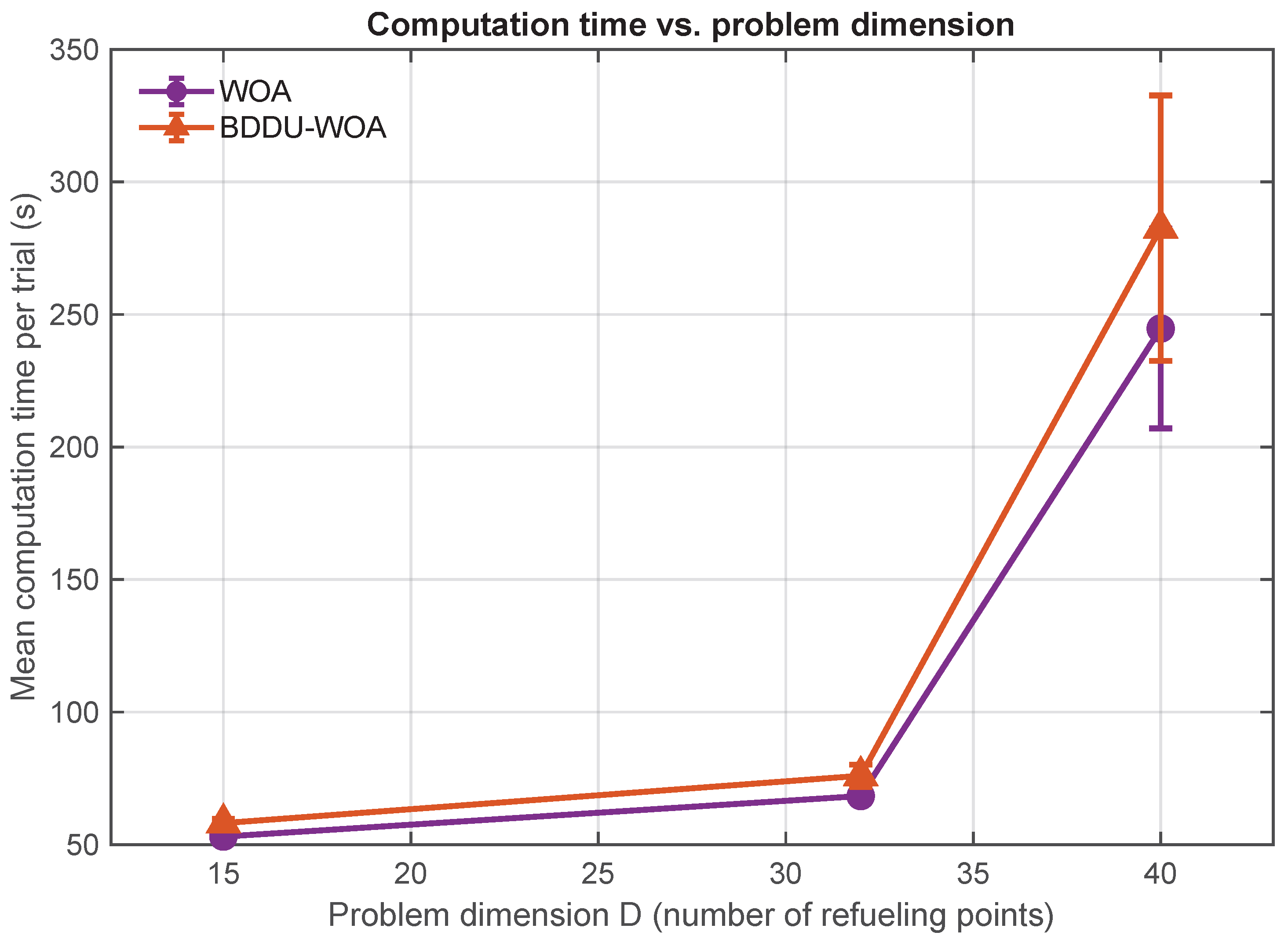
Figure 11 extends the cost analysis across all three test scenarios, showing how mean computation time scales with problem dimension D for both WOA and BDDU-WOA. The overhead remains approximately 10% across all scales (), confirming that BDDU’s bottleneck label extraction adds a near-constant factor rather than degrading the asymptotic scaling behavior.
Figure 11.
Mean computation time per trial as a function of problem dimension D. Error bars indicate ±1 standard deviation over 20 independent trials. BDDU-WOA’s overhead remains approximately 10% across all three problem scales, confirming that the bottleneck extraction mechanism introduces a near-constant cost factor without degrading asymptotic scalability.
5.7. Discussion and Limitations
Summary of findings:
- BDDU-WOA substantially improves feasibility (+40 pp mountain corridor; +60 pp at ablation), driven by bottleneck-aware dimension-wise step-size control with only two added parameters and an adaptive, parameter-free classification threshold.
- Bottleneck labels evolve as intended: CRITICAL dimensions dominate early iterations (∼50%) and reduce to ∼15% at convergence, while TIGHT and FREE each stabilize at ∼40–45%, confirming that the adaptive median-split maintains meaningful class occupancy throughout the search.
- Comprehensive robustness analysis (Experiment I) confirms statistical insensitivity of both and across their tested ranges (, ), persisting under 10% time window compression. The adaptive classification removes the need for threshold tuning entirely.
- Computational overhead is approximately 10%.
The distribution-driven classification (Section 4.3.1) addresses a structural weakness identified in earlier designs: a fixed absolute threshold concentrates nearly all dimensions in a single class when slackness values are inherently tight, degrading per-dimension differentiation. The median-split scheme guarantees that roughly half of all served dimensions are classified as TIGHT and half as FREE at every iteration, regardless of the slackness distribution. This ensures that the three bottleneck states always carry differentiated step-size prescriptions (, , 1), making the bottleneck-aware mechanism structurally robust.
Several limitations should be noted. The experiments compare against standard metaheuristics rather than dedicated bi-level solvers. The test scenarios are synthetically constructed, and the lower-level greedy scheduler may yield suboptimal bottleneck labels. Parameter robustness was demonstrated on NarrowDense benchmarks; confirmation on different topologies (e.g., hub-and-spoke) and on operational data remains future work. Extensions include nonlinear fuel consumption models (altitude, payload, weather) and integrated assignment–location optimization, both of which would require reformulating the current constraints.
6. Conclusions
This paper addressed the bi-level coupled scheduling problem for air refueling with continuous refueling point selection. We formulated a bi-level model that couples upper-level refueling point location with lower-level multi-tanker scheduling, and proposed the Bottleneck-Driven Decoupled Update (BDDU) strategy, which counters the coupling amplification effect through bottleneck-aware, per-dimension step-size control.
Key experimental findings: (i) BDDU-WOA substantially improves feasibility across all three test scenarios, with the largest gain on the coupling-intensive mountain corridor (+40 pp over WOA, ); (ii) ablation confirms the gain stems entirely from the single step-size control mechanism; (iii) a comprehensive robustness analysis spanning all BDDU and control parameters confirms that solution quality is statistically insensitive to all parameter choices (, ), enabling deployment without per-instance tuning; and (iv) computational overhead is roughly 10%.
On the primary objective of tanker sortie minimization, BDDU-WOA reduces mean tanker sorties from 7.1 to 6.8 (mountain corridor, 4.2%), 7.5 to 7.0 (16-route, 6.7%), and 19.6 to 19.4 (50-route, 1.0%). The largest relative improvement occurs in the moderately coupled scenario, where both algorithms achieve 100% feasibility but BDDU-WOA uses fewer tankers. In the high-dimensional scenario, BDDU-WOA’s primary advantage is the feasibility rate (65% vs. 25%) rather than tanker count reduction. WOA’s means reflect only 25–50% of trials (feasible subset); BDDU-WOA’s reflect 65–100%.
Several directions merit further investigation. Replacing the lower-level greedy scheduler with tabu search or column generation could sharpen the bottleneck labels. The BDDU design principle—bottleneck-aware decoupled updates driven by lower-level feedback—generalizes to other bi-level coupled combinatorial problems, including location-routing, network design with user equilibrium, and production–distribution coordination. Validation on operational data is the natural next step. For online use, BDDU’s bottleneck-aware mechanism could be embedded within a Model Predictive Control framework that replans from the current state at each cycle.
Author Contributions
Conceptualization: X.M. and F.Y.; methodology: X.M.; software: X.M.; validation: X.M.; formal analysis: X.M. and F.Y.; investigation: X.M.; resources: F.Y. and D.S.; data curation: X.M.; writing—original draft preparation: X.M.; writing—review and editing: D.S. and F.Y.; visualization: X.M.; supervision: F.Y. and D.S.; project administration: F.Y. and D.S.; funding acquisition: F.Y. and D.S. All authors have read and agreed to the published version of the manuscript.
Funding
This research received no external funding.
Institutional Review Board Statement
Not applicable.
Informed Consent Statement
Not applicable.
Data Availability Statement
The data presented in this study are available on request from the corresponding author.
Acknowledgments
The authors would like to thank the anonymous reviewers for their valuable comments and suggestions. During the preparation of this work, the authors used DeepSeek (version V4-Pro) for language polishing, translation assistance, code checking, and improvement suggestions. All core ideas, methodology design, mathematical modeling, experimental validation, and writing were completed by the authors. The AI-generated suggestions were selectively incorporated only after critical review and verification. After using this tool, the authors reviewed and edited the content as needed and take full responsibility for the content of the publication.
Conflicts of Interest
The authors declare no conflicts of interest.
Abbreviations
The following abbreviations are used in this manuscript:
| BDDU | Bottleneck-Driven Decoupled Update |
| WOA | Whale Optimization Algorithm |
| GWO | Grey Wolf Optimizer |
| PSO | Particle Swarm Optimization |
| MINLP | Mixed-Integer Nonlinear Programming |
| VRP | Vehicle Routing Problem |
| UAV | Unmanned Aerial Vehicle |
Appendix A
Figure A1.
BDDU-intrinsic parameter sensitivity profiles. (a) (maxStepCritical): mean score flat at 6.86 across 0.01–0.90. (b) (maxStepTight): modest score variation (6.75–7.05), , . (c) (timeWindowThreshold): mean score flat at 6.86 across 1–90 min. All panels show 100% feasibility rate (20/20 runs). Error bars: SD.
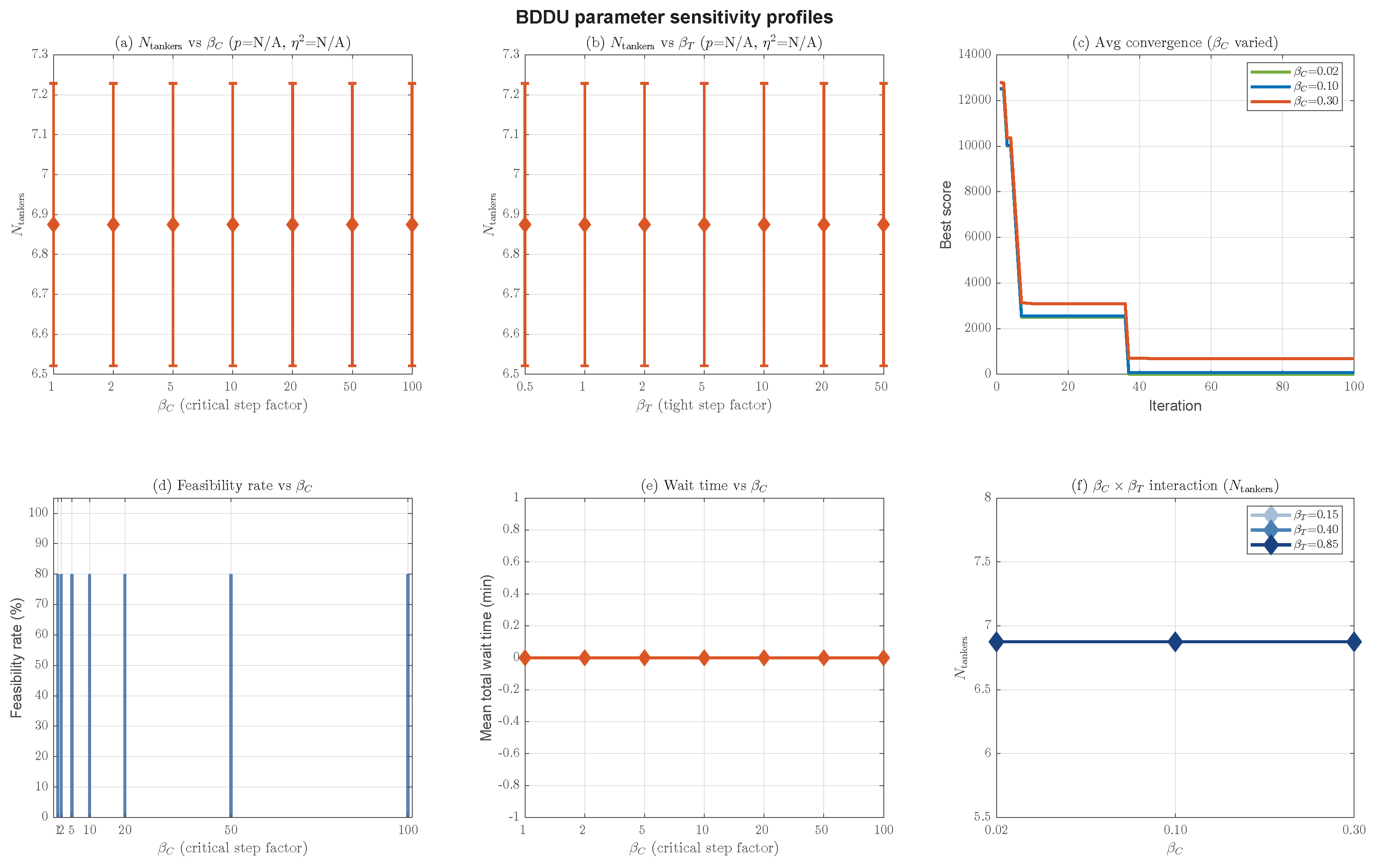
Table A1.
Algorithm control parameter sensitivity (ANOVA on ).
References
- Sundar, K.; Rathinam, S. Algorithms for Routing an Unmanned Aerial Vehicle in the Presence of Refueling Depots. IEEE Trans. Autom. Sci. Eng. 2014, 11, 287–294. [Google Scholar] [CrossRef] [Scilit]
- Kannon, T.E.; Nurre, S.G.; Lunday, B.J.; Hill, R.R. The Aircraft Routing with Air Refueling Problem: Exact and Greedy Approaches. In Proceedings of the IIE Annual Conference, Montreal, QC, Canada, 31 May–3 June 2014; p. 817. [Google Scholar]
- Kannon, T.E.; Nurre, S.G.; Lunday, B.J.; Hill, R.R. The Aircraft Routing Problem with Refueling. Optim. Lett. 2015, 9, 1609–1624. [Google Scholar] [CrossRef] [Scilit]
- Ferdowsi, F.; Maleki, H.R.; Rivaz, S. Air Refueling Tanker Allocation Based on a Multi-Objective Zero-One Integer Programming Model. Oper. Res. 2018, 20, 1913–1938. [Google Scholar] [CrossRef] [Scilit]
- Entz, R.M.; Scherer Schwening, G.; Fernandes de Oliveira, R. Application of Automatic Algorithm Generation to Air-to-Air Refueling Scheduling. In Proceedings of the 16th AIAA/ISSMO Multidisciplinary Analysis and Optimization Conference, Dallas, TX, USA, 22–26 June 2015. [Google Scholar]
- Hansknecht, C.; Joormann, I.; Korn, B.; Stiller, S.; Morscheck, F. Feeder Routing for Air-to-Air Refueling Operations. Eur. J. Oper. Res. 2023, 304, 779–796. [Google Scholar] [CrossRef] [Scilit]
- Toydas, M.; Saraç, M.T. A Mixed Integer Nonlinear Model for Air Refueling Optimization to Save Fuel in Military Deployment Operations. Int. J. Ind. Eng. Theory Appl. Pract. 2020, 27, 627–644. [Google Scholar]
- Toydas, M.; Malyemez, C. Air Refueling Optimisation for More Agile and Efficient Military Deployment Operations. Aeronaut. J. 2021, 126, 365–380. [Google Scholar] [CrossRef] [Scilit]
- Tan, R.; Gan, X.; Wu, N.; Chen, Z. Location Method of Refueling Airspace in Air Combat Based on Modified AFS Algorithm. In Proceedings of the 2022 IEEE 5th International Conference on Automation, Electronics and Electrical Engineering (AUTEEE), Shenyang, China, 18–20 November 2022; pp. 929–934. [Google Scholar]
- Zhang, Z.; Huang, Z.; Liu, X.; Feng, B. Research on Multiple Air-to-Air Refueling Planning Based on Multi-Dimensional Improved NSGA-II Algorithm. Electronics 2023, 12, 3880. [Google Scholar] [CrossRef] [Scilit]
- Wang, Y.; Zhang, J.; Liu, H. Bi-Level Optimization for Aerial Refueling Mission Planning Under Complex Constraints. Eur. J. Oper. Res. 2024, 318, 445–462. [Google Scholar]
- Zhang, H.; Li, W.; Chen, X. Bridging Game Theory and Multi-Agent Systems: Development Status and Future Prospects. Prog. Aerosp. Sci. 2026, 132, 101183. [Google Scholar] [CrossRef] [Scilit]
- Wang, J.; Liu, Y.; Zhao, T. Resilient Control Under DoS Attacks of Hybrid Air–Sea Swarms with Cooperative–Competitive Interactions. IEEE Trans. Aerosp. Electron. Syst. 2025, 61, 1823–1838. [Google Scholar] [CrossRef] [Scilit]
- Mirjalili, S.; Lewis, A. The Whale Optimization Algorithm. Adv. Eng. Softw. 2016, 95, 51–67. [Google Scholar] [CrossRef] [Scilit]
- Mirjalili, S.; Mirjalili, S.M.; Lewis, A. Grey Wolf Optimizer. Adv. Eng. Softw. 2014, 69, 46–61. [Google Scholar] [CrossRef] [Scilit]

Disclaimer/Publisher’s Note: The statements, opinions and data contained in all publications are solely those of the individual author(s) and contributor(s) and not of MDPI and/or the editor(s). MDPI and/or the editor(s) disclaim responsibility for any injury to people or property resulting from any ideas, methods, instructions or products referred to in the content. |
© 2026 by the authors. Licensee MDPI, Basel, Switzerland. This article is an open access article distributed under the terms and conditions of the Creative Commons Attribution (CC BY) license.