A Novel Strong-Form Zonal Free Element Method Based on Lagrange Interpolation for Vibro-Acoustic Coupling Analysis

Abstract

A novel strong-form meshless method based on Lagrange interpolation is proposed for vibro-acoustic coupling analysis. The governing equations of acoustic and structural domains, together with the coupling interface conditions, are discretized directly in differential form without relying on predefined meshes, thereby improving geometric flexibility. The computational domain is partitioned into local subdomains, within which Lagrange interpolation is employed to construct approximation functions from nodal distributions. In this manner, the proposed framework combines the flexibility of meshless formulations with a zonal parameterization strategy similar to that used in isogeometric analysis. Moreover, spatial derivatives and system matrices are directly evaluated and assembled at nodal points, avoiding numerical integration and simplifying the implementation procedure. Owing to the Kronecker delta property of Lagrange polynomials, boundary conditions can be imposed accurately and conveniently. For transient analysis, the Newmark-$\beta$ scheme is adopted to integrate both first- and second-order temporal terms, ensuring stable and accurate time integration. Finally, numerical examples, including comparisons with commercial software, demonstrate the accuracy and effectiveness of the proposed method for complex vibro-acoustic problems.

1. Introduction

Extremely high acoustic loads, with sound pressure levels up to 180 dB [1], are often imposed on turbine blades, struts, and other critical engine components. Such intense acoustic excitation can severely threaten structural integrity and shorten fatigue life. In high-intensity noise environments, rapidly fluctuating stresses are likely to induce the initiation and propagation of fatigue cracks, eventually leading to structural failure [2]. Therefore, reliable numerical methods are required to accurately predict the vibro-acoustic response of such structures.

In structural vibration analysis, numerical methods such as the finite element method (FEM) [3] and the boundary element method (BEM) [4] have been widely used. For instance, the nonlinear response of aerospace structures under random excitation was analyzed by Vaicaiti [5] using a combination of the Galerkin method and the Monte Carlo approach. Zhang et al. [6] applied FEM to the X-43 model to investigate vibro-acoustic coupling, and the deviations between the first ten natural frequencies and experimental results were within 5%, with most modes showing errors below 1%. BEM provides clear advantages in modeling unbounded acoustic fields and multi-scale thermal protection structures [7], as only the boundaries need to be discretized. To handle vibro-acoustic problems of wings, a hybrid FEM–BEM algorithm was developed by Djojodihardjo [8]. Zheng et al. [9] combined BEM with the element differential method to simulate thermo-mechanical coupling in combustor cooling channels with coatings.

With the advancement of numerical techniques, problems in acoustics and structural dynamics have increasingly been solved using advanced approaches, such as the element differential method (EDM) [10], the discontinuous Galerkin method (DGM) [11], and the virtual element method (VEM) [12]. The free element method (FREM), proposed by Gao et al. [13], is a meshless collocation technique distinguished from other meshless methods [14] by constructing isoparametric interpolations through local collocation elements. In FREM, shape functions are employed for interpolation in a manner similar to FEM, which ensures good approximation properties.

Essential boundary conditions can be handled more easily in FREM than in meshless Galerkin methods [15], which provides higher stability and robustness for multi-physics interface coupling. It is worth noting that for meshfree collocation formulations, the resulting system matrices are generally non-symmetric, especially in transient analyses. This may raise important issues regarding numerical stability and modal properties. Recent work by [16] has shown that, for least-squares meshfree collocation methods, the symmetry of the formulation is lost in transient problems, which may lead to complex eigenvalues and affect stability. These findings highlight the necessity of carefully assessing the stability characteristics of strong-form meshfree methods in time-domain simulations. In the present work, this aspect is examined through transient numerical examples.

The FREM has achieved notable success in analyzing piezoelectric materials [17], thermoelastic behavior of functional materials [18], and internal or external flow problems [19,20]. Gao et al. [21] proposed the domain partitioning concept to simplify modeling in multi-material and multi-physics coupling systems. This approach makes mesh generation and interface treatment more efficient.

In this work, a zonal free element method (ZFREM) is developed for time-domain vibro-acoustic coupling analysis. The method adopts a zonal decomposition strategy combined with a strong-form meshless formulation based on Lagrange interpolation, providing a flexible framework for complex coupled systems. The governing equations are directly discretized in differential form over both acoustic and structural domains as well as their interfaces, avoiding the need for numerical integration required in conventional weak-form or mesh-dependent approaches. A node-wise construction strategy is employed within each subdomain to evaluate spatial derivatives and assemble system matrices efficiently. In addition, boundary quantities are consistently determined from governing boundary equations, ensuring a stable treatment of interface and boundary conditions.

The remainder of this paper is organized as follows. Section 2 introduces the fundamental theory of vibro-acoustic coupling, providing the theoretical basis for the subsequent analysis. In Section 3, the discretization procedure based on ZFREM is described in detail, highlighting its implementation and advantages. Section 4 presents numerical examples to demonstrate the reliability and effectiveness of the proposed approach. Finally, Section 5 summarizes the main findings and draws conclusions.

2. Mathematical Formulation of Vibro-Acoustic Coupling

2.1. Governing Equations of the Acoustic Domain

The governing equation of the acoustic domain is given by the classical wave equation:

$$\nabla ·\left({\displaystyle \frac{1}{{\rho }_{\alpha }}}\nabla p\right)-{\displaystyle \frac{1}{{\rho }_{\alpha }{c}^2}}{\displaystyle \frac{{\partial }^{2}p}{\partial t^2}}=-q,$$

(1)

where p denotes the acoustic pressure, c is the speed of sound, ${\rho }_{\alpha }$ is the medium density, and q represents the internal acoustic source term.

The boundary conditions associated with Equation (1) are summarized as follows. On the acoustic pressure boundary ${\mathsf{\Gamma }}_p$, the pressure p is prescribed as

$$p=\overline{p},$$

(2)

where $\overline{p}=0$ corresponds to an acoustically soft boundary, in which the incident wave is reflected with equal amplitude but opposite phase.

On the normal acceleration boundary ${\mathsf{\Gamma }}_a$, the normal acceleration $a_n$ of the medium is specified as

$${\displaystyle \frac{1}{{\rho }_{\alpha }}}{\displaystyle \frac{\partial p}{\partial \mathit{n}}}={\overline{a}}_n,$$

(3)

which is derived from the momentum conservation equation relating the pressure gradient to fluid acceleration. Here, $\mathit{n}$ denotes the unit normal vector on the vibro-acoustic interface, which is consistently defined as pointing from the solid domain to the acoustic domain. This convention is used consistently in both the acoustic and structural governing equations to ensure sign consistency in the coupling conditions. When ${\overline{a}}_n=0$, ${\mathsf{\Gamma }}_a$ represents an acoustically hard boundary, for which the wave is reflected with the same amplitude and phase.

On the impedance boundary ${\mathsf{\Gamma }}_z$, the acoustic impedance Z is prescribed as

$${\displaystyle \frac{1}{{\rho }_{\alpha }}}{\displaystyle \frac{\partial p}{\partial \mathit{n}}}={\displaystyle \frac{1}{Z}}{\displaystyle \frac{\partial p}{\partial t}},$$

(4)

which relates the normal particle velocity to the acoustic pressure through the impedance Z. When Z equals the characteristic impedance of the medium, $Z={\rho }_{\alpha }c$, the boundary becomes non-reflecting, such that the incident acoustic waves are fully absorbed without affecting the computational domain.

2.2. Governing Equations of the Solid Domain

The governing equation of the linear elastic solid domain [22] is expressed as

$${\displaystyle \frac{\partial {\sigma }_{ij}}{\partial x_j}}-{\rho }_s{\displaystyle \frac{{\partial }^2{u}_i}{\partial t^2}}-\mu {\displaystyle \frac{\partial u_i}{\partial t}}=-b_i, i=1,\dots ,m,$$

(5)

where ${\sigma }_{ij}$ is the stress tensor, ${\rho }_s$ is the material density, $\mu$ is the damping coefficient, $b_i$ denotes the body force, and m is the spatial dimension of the problem. Repeated indices imply summation according to the Einstein summation convention.

The stress tensor ${\sigma }_{ij}$ is related to the strain tensor ${\epsilon }_{kl}$ through the constitutive relation

$${\sigma }_{ij}=D_{ijkl}\left(\mathbf{x}\right) {\epsilon }_{kl},$$

(6)

where $D_{ijkl}\left(\mathbf{x}\right)$ is the elastic constitutive tensor, which may vary spatially.

The strain tensor ${\epsilon }_{kl}$ is defined in terms of the displacement field $u_i$ as

$${\epsilon }_{kl}={\displaystyle \frac{1}{2}}\left({\displaystyle \frac{\partial u_k}{\partial x_l}}+{\displaystyle \frac{\partial u_l}{\partial x_k}}\right).$$

(7)

By substituting Equations (7) and (6) into Equation (5), the governing equation can be written as

$$D_{ijkl}{\displaystyle \frac{{\partial }^2{u}_k}{\partial x_l\partial x_j}}+{\displaystyle \frac{\partial D_{ijkl}}{\partial x_j}}{\displaystyle \frac{\partial u_k}{\partial x_l}}-{\rho }_s{\displaystyle \frac{{\partial }^2{u}_i}{\partial t^2}}-\mu {\displaystyle \frac{\partial u_i}{\partial t}}=-b_i.$$

(8)

The boundary conditions associated with Equation (8) are defined as follows. On the displacement boundary ${\mathsf{\Gamma }}_u$, the displacement is prescribed:

$$u_i={\overline{u}}_i.$$

(9)

On the traction boundary ${\mathsf{\Gamma }}_t$, the traction is specified as

$${\sigma }_{ij}{n}_j={\overline{t}}_i.$$

(10)

Substituting Equations (6) and (7) into Equation (10) yields

$$D_{ijkl}{n}_j{\displaystyle \frac{\partial u_k}{\partial x_l}}={\overline{t}}_i.$$

(11)

The initial conditions for the coupled vibro-acoustic system are expressed as

$$\left\{\begin{array}{c}p(\mathit{x},0)=\overline{p}\left(\mathit{x}\right),\hfill \\ p_{,t}(\mathit{x},0)={\overline{p}}_{,t}\left(\mathit{x}\right),\hfill \\ u_i(\mathit{x},0)={\overline{u}}_i\left(\mathit{x}\right),\hfill \\ u_{i,t}(\mathit{x},0)={\overline{u}}_{i,t}\left(\mathit{x}\right),\hfill \end{array}\right.$$

(12)

where $p_{,t}={\displaystyle \frac{\partial p}{\partial t}}$ and $u_{i,t}={\displaystyle \frac{\partial u_i}{\partial t}}$ denote time derivatives.

2.3. Coupling Equations at the Interface

At the interface between the acoustic and solid domains, an m-dimensional problem involves $m+1$ unknowns: the displacement components in each spatial direction and the acoustic pressure. The coupling conditions among these variables include:

The particle accelerations on both sides of the interface are identical. Taking Equation (3) into account, the coupling equation can be expressed as

$${\displaystyle \frac{1}{{\rho }_{\alpha }}}{\displaystyle \frac{\partial p}{\partial \mathit{n}}}={\displaystyle \frac{{\partial }^2{u}_n}{\partial t^2}},$$

(13)

where $u_n=u_i{n}_i$ denotes the normal component of the displacement along the interface normal direction. The traction exerted on the solid domain is equal to the acoustic pressure in the acoustic domain. According to Equation (11), the coupling equation is given by

$$D_{ijkl}{n}_j{\displaystyle \frac{\partial u_k}{\partial x_l}}=-n_{i}p.$$

(14)

3. Numerical Discretization

3.1. Computational Domain Discretization Method

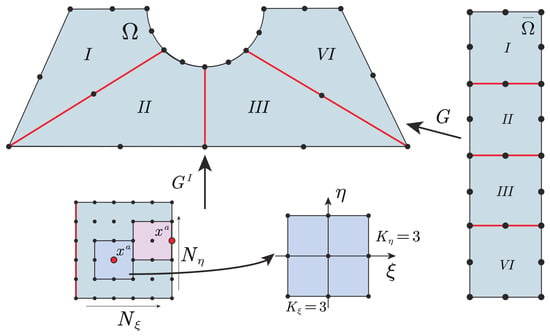
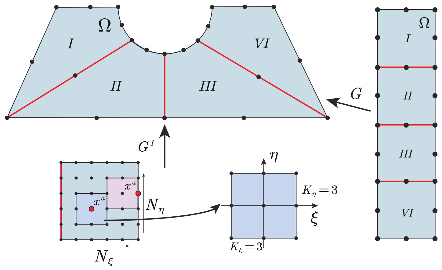
In vibro-acoustic coupling analysis, complex geometries and multi-material configurations are handled by first dividing the computational domain into a set of simpler subdomains. An illustrative example of this subdivision is provided in Figure 1. Each subdomain is subsequently mapped to a standard reference domain $\overline{\mathsf{\Omega }}$ through a geometric transformation $G:\overline{\mathsf{\Omega }}\to \mathsf{\Omega }$. Within each reference subdomain $\overline{\mathsf{\Omega }}$, a structured distribution of nodes is introduced in the form of a uniform $N_{\xi }\times N_{\eta }$ grid, where $N_{\xi }$ and $N_{\eta }$ denote the numbers of nodes in each coordinate direction. Based on the nodal distribution, the collocation nodes are classified into interior, boundary, and interface nodes according to their locations. For each node, a local interpolation domain is constructed by selecting its neighboring nodes, forming a local collocation element in a node-wise manner. Such local elements are generated adaptively for each node, rather than being predefined as in conventional element-based methods. As a result, the present formulation avoids the need for global mesh connectivity and element topology, while retaining the flexibility of node-based approximation and the geometric adaptability of local interpolation. This characteristic enables the method to effectively handle complex geometries and multi-domain coupling problems within a unified framework.

Figure 1. Schematic illustration of domain partitioning and collocation element generation.

As depicted in Figure 1, a collocation element is generated for each node $x^a$ in the reference subdomain $\overline{\mathsf{\Omega }}$ by incorporating the node together with its surrounding points. This procedure gives rise to a local Lagrangian element containing $K_{\xi }\times K_{\eta }$ nodes in two-dimensional cases. The element shape functions $N_{\alpha }$ are derived from one-dimensional Lagrange interpolation polynomials.

$$x_i=N_{\alpha }{x}_i^{\alpha },$$

(15)

$$p=N_{\alpha }{p}^{\alpha },$$

(16)

$$u_i=N_{\alpha }{u}_i^{\alpha }.$$

(17)

The element shape functions $N_{\alpha }$ are derived from one-dimensional Lagrange interpolation polynomials. For a one-dimensional local coordinate $\xi$, the Lagrange interpolation polynomial associated with node $\alpha$ is given by

$$N_{\alpha }\left(\xi \right)={\mathsf{\Pi }}_{\beta =1,\beta \ne \alpha }^k{\displaystyle \frac{\xi -{\xi }^{\beta }}{{\xi }^{\alpha }-{\xi }^{\beta }}}.$$

(18)

For two-dimensional cases, the shape functions are constructed by tensor-product expansion as

$$N_{\alpha }(\xi ,\eta )=N_i\left(\xi \right)N_j\left(\eta \right),$$

(19)

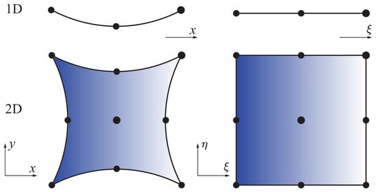
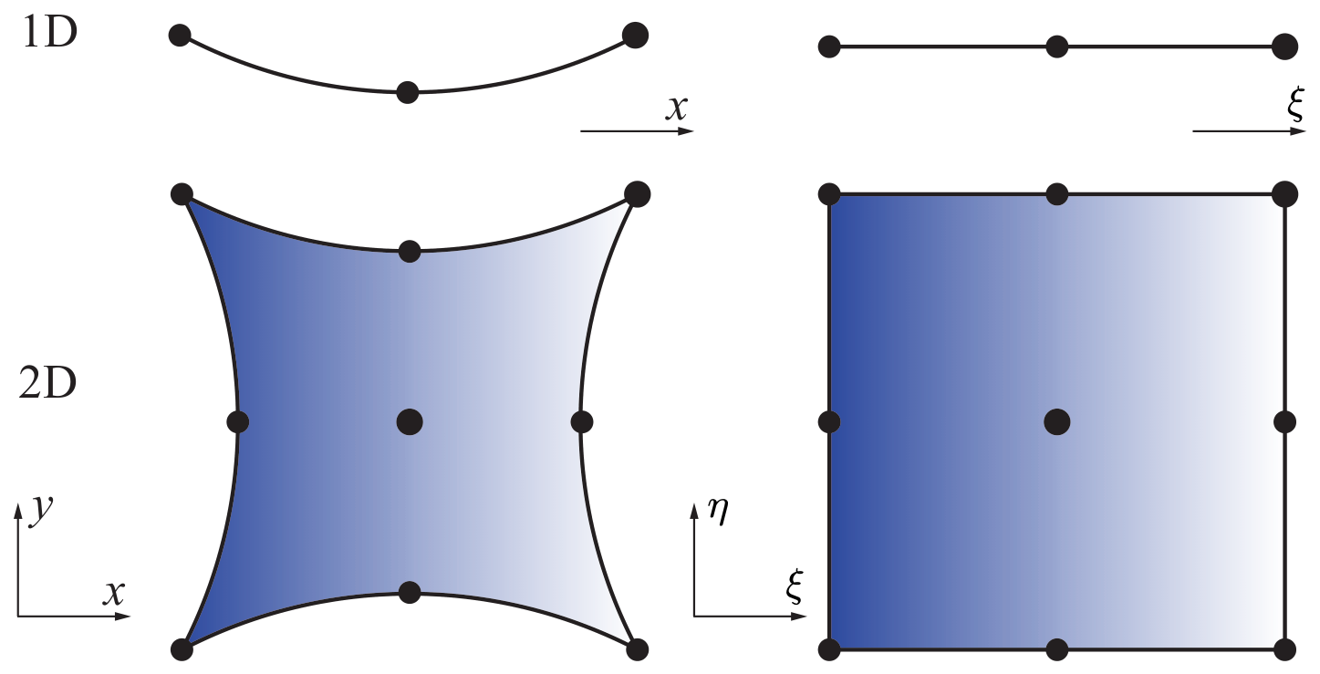
where $\alpha$ corresponds to the node index associated with the pair $(i,j)$. The mapping relationship for the three-node and nine-node Lagrange interpolation elements is shown in Figure 2.

Figure 2. Mapping of three-node and nine-node Lagrange interpolation elements between local and physical coordinate systems.

In the above equation, $N_{\alpha }$ denotes the shape function of node $\alpha$ within the local collocation element, which is an explicit function of the local coordinates ${\xi }_i$. Using the chain rule, the derivatives of the shape functions with respect to the spatial coordinates, ${\displaystyle \frac{\partial N_{\alpha }}{\partial x_i}}$ and ${\displaystyle \frac{{\partial }^2{N}_{\alpha }}{\partial x_i\partial x_j}}$, can be obtained (for computational details, see [13]). Then, the derivatives of an arbitrary nodal variable $\varphi$ with respect to the spatial coordinates can be calculated as

$${\displaystyle \frac{\partial \varphi }{\partial x_i}}={\displaystyle \frac{\partial N_{\alpha }}{\partial x_i}}{\varphi }^{\alpha },$$

(20)

$${\displaystyle \frac{{\partial }^2\varphi }{\partial x_i{x}_j}}={\displaystyle \frac{{\partial }^2{N}_{\alpha }}{\partial x_i{x}_j}}{\varphi }^{\alpha }.$$

(21)

For a homogeneous medium, substituting Equations (20) and (21) into the governing equation of the acoustic field (Equation (1)) yields the discrete equations for the nodal variables within the domain.

$${\displaystyle \frac{1}{{\rho }_{\alpha }}}{\displaystyle \frac{{\partial }^2{N}_{\alpha }\left(\xi \right)}{\partial x_i\partial x_i}}{p}^{\alpha }-{\displaystyle \frac{1}{{\rho }_{\alpha }{c}^2}}{\displaystyle \frac{{\partial }^{2}p\left(\mathit{x}\right)}{\partial t^2}}=-q\left(\mathit{x}\right).$$

(22)

For the internal subdomain interfaces within the acoustic field, both sides belong to the same medium, while multiple interfaces may intersect at corner points. Therefore, the normal accelerations on the two sides should be equal in magnitude but opposite in direction, and their sum is zero. According to Equation (3), this condition can be expressed as

$${\displaystyle \sum _{f=1}^M}-{\displaystyle \frac{1}{{\rho }_{\alpha }}}{\displaystyle \frac{\partial N_{\alpha }\left({\xi }^I\right)}{\partial x_i}}{n}_i^f\left({\xi }^I\right)p^{\alpha }=0,$$

(23)

where M denotes the number of interface segments associated with node ${\xi }^I$. $n_i^f$ denotes the outward normal direction of interface f. For physical boundaries, the discrete equations can be obtained by substituting Equations (20) and (21) into the corresponding boundary condition relations.

For the solid domain, the governing equations at internal nodes are discretized as follows:

$$\left[D_{ijkl}\left(\mathit{\xi }\right){\displaystyle \frac{{\partial }^2{N}_{\alpha }\left(\mathit{\xi }\right)}{\partial x_l\partial x_j}}+{\displaystyle \frac{\partial N_{\beta }\left(\mathit{\xi }\right)}{\partial x_j}}{D}_{ijkl}^{\beta }{\displaystyle \frac{\partial N_{\alpha }\left(\mathit{\xi }\right)}{\partial x_l}}\right]u_k^{\alpha }-{\rho }_s{\displaystyle \frac{{\partial }^2{u}_i\left(\mathit{x}\right)}{\partial t^2}}-\mu {\displaystyle \frac{\partial u_i\left(\mathit{x}\right)}{\partial t}}=-b_i\left(\mathit{x}\right).$$

(24)

where $\mathit{\xi }$ denotes the local coordinates of the internal collocation point within the subdomain, with $\mathit{\xi }=(\xi ,\eta )$ for two-dimensional problems, and $D_{ijkl}^{\beta }$ represents the generalized elastic matrix associated with node $\beta$.

Similarly, for internal interfaces within the solid domain, the discrete equations can be obtained based on the balance of tractions on both sides as

$${\displaystyle \sum _{f=1}^M}{D}_{ijkl}\left({\mathit{\xi }}^I\right){\displaystyle \frac{\partial N_{\alpha }\left({\mathit{\xi }}^I\right)}{\partial x_i}}{n}_j^f\left({\mathit{\xi }}^I\right)u_k^{\alpha }=0,$$

(25)

where $n_i^{\left(f\right)}\left({\mathit{\xi }}^I\right)$ denotes the unit normal vector of the f-th boundary segment at the collocation point. All normal vectors are consistently defined to point from the solid domain to the acoustic domain.

For the points located on the physical boundary, the discrete equations can be obtained by directly substituting Equations (20) and (21) into the corresponding boundary condition relations. On the vibro-acoustic coupling boundary, the discrete equations can be obtained from Equations (13) and (14), respectively, as follows:

$${\displaystyle \sum _{f=1}^M}-{\displaystyle \frac{1}{{\rho }_a}}{\displaystyle \frac{\partial N_{\alpha }\left({\mathit{\xi }}^I\right)}{\partial x_i}}{n}_i^f\left({\mathit{\xi }}^I\right)p^{\alpha }=-n_j{\displaystyle \frac{{\partial }^2{u}_j}{\partial t^2}},$$

(26)

$${\displaystyle \sum _{f=1}^M}{D}_{ijkl}\left({\mathit{\xi }}^I\right){\displaystyle \frac{\partial N_{\alpha }\left({\mathit{\xi }}^I\right)}{\partial x_l}}{n}_i^f\left({\mathit{\xi }}^I\right)u_k^{\alpha }=-n_{j}p.$$

(27)

It should be noted that the above formulation applies exclusively to the vibro-acoustic coupling interface.

3.2. Time Discretization

Following spatial discretization, the governing equations are transformed into the semi-discrete system of the following form:

$$\left[\begin{array}{cc}{\mathit{M}}_{uu}& 0\\ {\mathit{M}}_{pu}& {\mathit{M}}_{pp}\end{array}\right]\left[\begin{array}{c}\ddot{\mathit{u}}\\ \ddot{\mathit{p}}\end{array}\right]+\left[\begin{array}{cc}{\mathit{C}}_{uu}& 0\\ 0& {\mathit{C}}_{pp}\end{array}\right]\left[\begin{array}{c}\dot{\mathit{u}}\\ \dot{\mathit{p}}\end{array}\right]+\left[\begin{array}{cc}{\mathit{K}}_{uu}& {\mathit{K}}_{up}\\ 0& {\mathit{K}}_{pp}\end{array}\right]\left[\begin{array}{c}\mathit{u}\\ \mathit{p}\end{array}\right]=\mathit{F}.$$

(28)

The above equations show that, besides spatial derivative terms, the governing equations and boundary conditions of both the acoustic and elastic fields also contain temporal derivatives. In this work, both the first- and second-order time derivatives are approximated using the Newmark-$\beta$ method [22],

$${\ddot{\varphi }}_{t+\Delta t}={\displaystyle \frac{1}{\alpha \Delta {\mathrm{t}}^2}}\left({\varphi }_{t+\Delta t}-{\varphi }_t\right)-{\displaystyle \frac{1}{\alpha \Delta \mathrm{t}}}{\dot{\varphi }}_t-\left({\displaystyle \frac{1}{2\alpha }}-1\right){\ddot{\varphi }}_t,$$

(29)

$${\dot{\varphi }}_{t+\Delta t}={\displaystyle \frac{\delta }{\alpha \Delta \mathrm{t}}}\left({\varphi }_{t+\Delta t}-{\varphi }_t\right)+\left(1-{\displaystyle \frac{\delta }{\alpha }}\right){\dot{\varphi }}_t+\left(1-{\displaystyle \frac{\delta }{2\alpha }}\right)\Delta t{\ddot{\varphi }}_t.$$

(30)

In the present work, the parameters are chosen as $\alpha =0.25$ and $\delta =0.5$, corresponding to the constant average acceleration scheme. This choice ensures unconditional stability for linear problems and is widely used in transient dynamic analysis. It is worth noting that the Newmark method is unconditionally stable for linear problems when the parameters satisfy $\delta \ge 0.5$ and $\alpha \ge {\displaystyle \frac{1}{4}}{(\delta +0.5)}^2$, indicating that the stability of the solution is independent of the time step size $\Delta t$. The potential $\varphi$ is replaced by the acoustic pressure p and the displacement components $u_i$. These quantities are then substituted into the semi-discrete equations of the acoustic and structural fields to obtain the final discrete system.

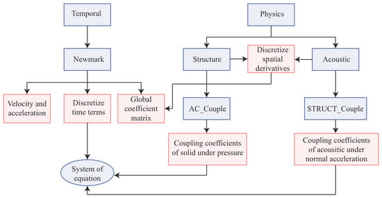
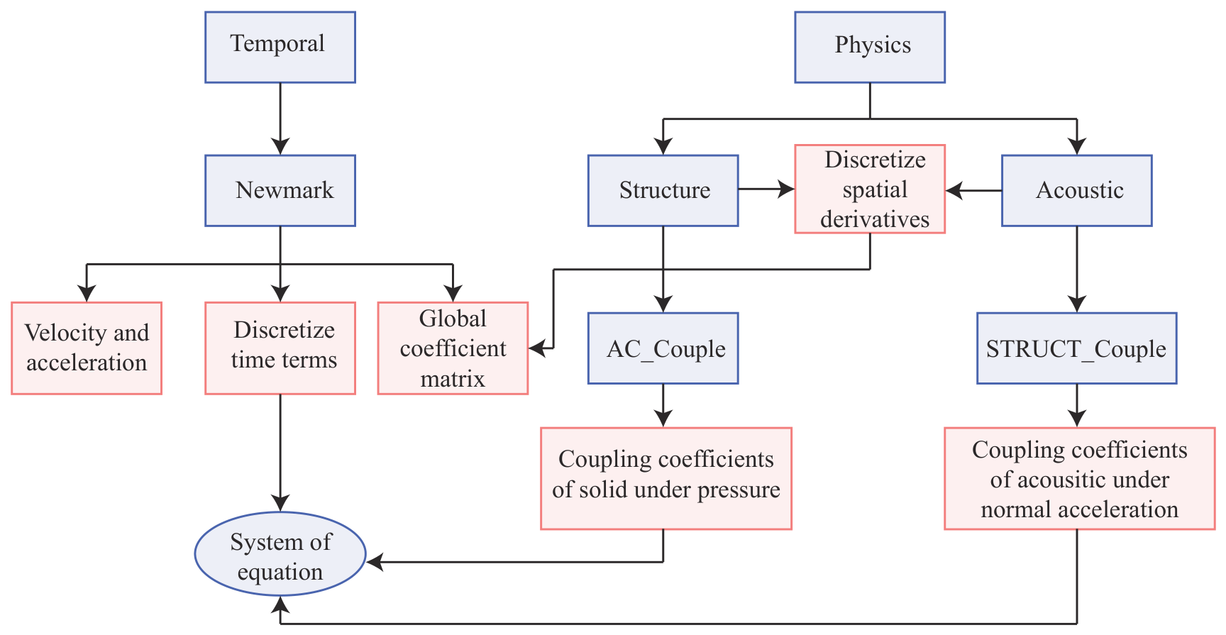
As illustrated in Figure 3, the framework consists of two core modules: the temporal iteration module (Temporal) and the physical field module (Physics). These modules are responsible for time integration and the computation of physical field variables, respectively. Both modules are derived from a common base class, and different types of computations are realized by overloading the internal functions.

Figure 3. Flowchart of the vibro-acoustic coupling computation in the ZFREM framework.

4. Numerical Examples and Discussion

4.1. A Channel Model with Two Elastic Ribs

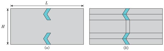
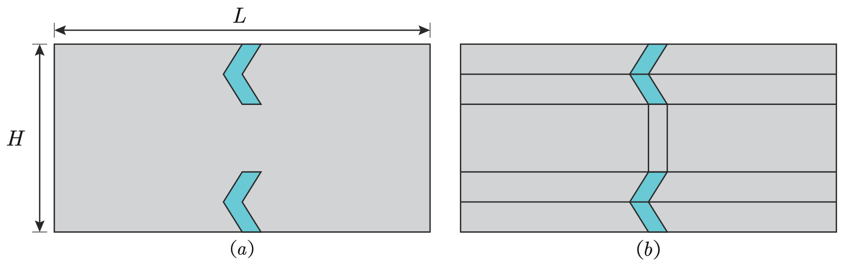
The schematic diagram of the channel model is shown in Figure 4a. The channel contains two elastic ribs, where the blue regions represent the ribs and the gray regions denote air. The overall dimensions of the channel are $L=10 \mathrm{m}$ in length and $H=5 \mathrm{m}$ in height. The medium inside the channel is air, with a density of $1 \mathrm{kg}/{\mathrm{m}}^3$ and a sound speed of $340 \mathrm{m}/\mathrm{s}$. The elastic material has a density of $7000 {\mathrm{kg}/\mathrm{m}}^3$, a Young’s modulus of $2 \mathrm{GPa}$, and a Poisson’s ratio of $0.3$. Initially, the air pressure is zero and the elastic ribs are at rest. The time step used in the simulations is $\Delta t=0.001$, and the total simulation time is $T=0.1$. Unless otherwise specified, the viscous damping coefficient $\mu$ is taken as zero in the following numerical examples. At $t=0$, a sinusoidal pressure is imposed at the left boundary of the channel, with an amplitude of $10 \mathrm{kPa}$ and a frequency of $100 \mathrm{Hz}$. A non-reflecting boundary condition is applied to the right end of the channel, while the upper and lower boundaries are modeled as rigid walls.

Figure 4. Schematic of the duct model: (a) Geometry of the channel. (b) Zonal domain of the channel.

The computational domain is partitioned as shown in Figure 4b, followed by node discretization. Three levels of spatial discretization with different node densities are employed in ZFREM to examine convergence behavior. The coarse discretization contains 1395 nodes, including 182 nodes in the solid domain and 1213 nodes in the acoustic domain. The medium discretization consists of 7171 nodes, with 870 nodes in the solid domain and 6301 nodes in the acoustic domain. The fine discretization contains 20,691 nodes, including 2450 nodes in the solid domain and 18,241 nodes in the acoustic domain. To assess the accuracy of the proposed method, the COMSOL Multiphysics 6.3 (COMSOL AB, Stockholm, Sweden) results obtained with a sufficiently refined mesh are taken as reference solutions. In COMSOL, 27,898 quadratic triangular elements are employed, yielding a total of 59,897 nodes.

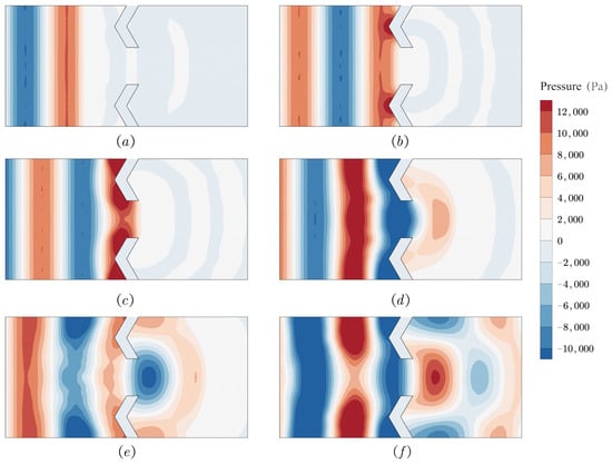
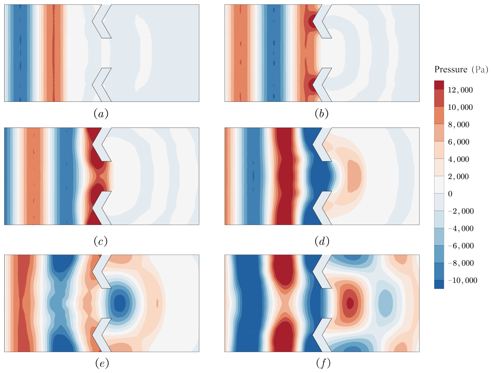
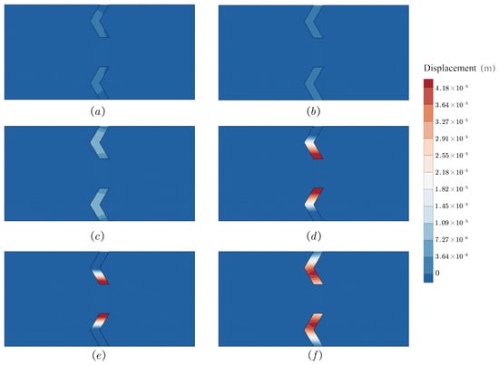
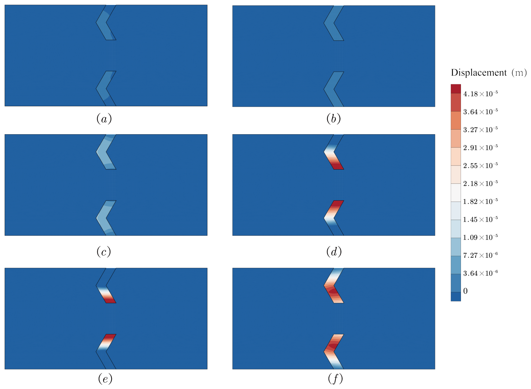
Figure 5 and Figure 6 present the distributions of acoustic pressure and solid displacement at six different time instants. Figure 5a–f and Figure 6a–f correspond to $t=0.01 \mathrm{s}$, $0.015 \mathrm{s}$, $0.017 \mathrm{s}$, $0.022 \mathrm{s}$, $0.025 \mathrm{s}$, and $0.031 \mathrm{s}$, respectively. Initially, the incident wavefront is planar. As the wave propagates through the opening between the elastic ribs, diffraction effects are clearly observed. Upstream of the elastic ribs, part of the acoustic wave is reflected due to the obstruction of the solid structures, resulting in significant modifications of the acoustic field. Meanwhile, the displacement field in the solid domain exhibits pronounced vibration near the elastic ribs, driven by the incident acoustic waves. The spatial distribution of displacement is closely correlated with the acoustic pressure field, reflecting the coupled vibro-acoustic behavior. These results clearly demonstrate the wave scattering and diffraction induced by the elastic obstacles, as well as the dynamic response of the solid structure.

Figure 5. Snapshots of acoustic pressure distributions at different time instants: (a) $t=0.01$ s. (b) $t=0.015$ s. (c) $t=0.017$ s. (d) $t=0.022$ s. (e) $t=0.025$ s. (f) $t=0.031$ s.

Figure 6. Snapshots of displacement distributions in the solid domain at different time instants: (a) $t=0.01$ s. (b) $t=0.015$ s. (c) $t=0.017$ s. (d) $t=0.022$ s. (e) $t=0.025$ s. (f) $t=0.031$ s.

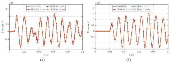
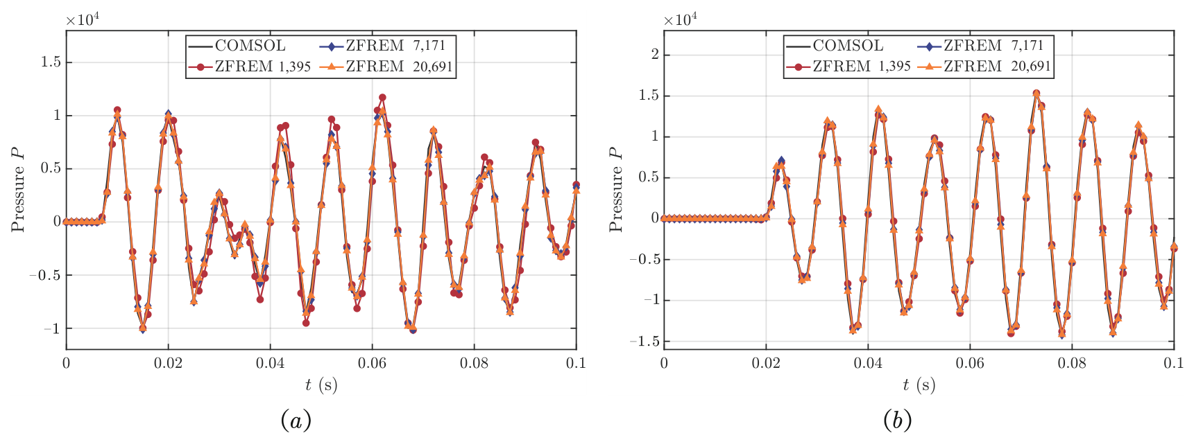
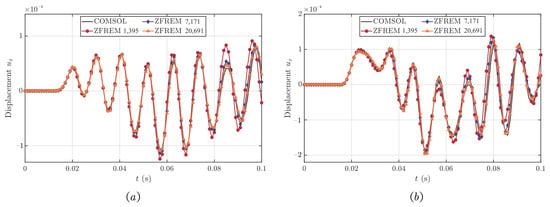
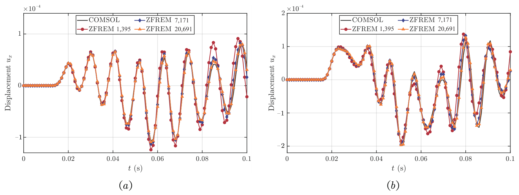
Figure 7 and Figure 8 show the temporal variations in acoustic pressure and solid displacement at selected nodes. Even with the coarsest mesh, the acoustic pressure closely matches the reference solution, while the medium and fine meshes yield results nearly identical to COMSOL. For solid displacement, noticeable discrepancies appear under the coarse mesh, but the errors rapidly decrease with increasing nodal density. This behavior is primarily due to the elastic wave speed in the solid being an order of magnitude higher than the sound speed in air, resulting in shorter wavelengths and higher spatial resolution requirements. ZFREM can effectively resolve these high-frequency elastic waves by uniformly refining the node distribution, ensuring accurate representation of the coupled vibro-acoustic response.

Figure 7. Variations in acoustic pressure at different nodes: (a) Node (2.50, 2.50). (b) Node (7.00, 2.50).

Figure 8. Variations in the displacement in the x-direction at different nodes: (a) Node (4.50, 4.13). (b) Node (5.00, 3.27).

Overall, Figure 5, Figure 6, Figure 7 and Figure 8 demonstrate that the proposed ZFREM accurately captures both acoustic and structural responses. The method exhibits excellent convergence with increasing nodal density, reliably reproduces high-frequency elastic wave behavior, and effectively resolves the coupled vibro-acoustic dynamics, even under coarse discretization. These results confirm the capability of ZFREM to achieve high accuracy in representing complex vibro-acoustic problems, with controllable nodal refinement enabling flexible resolution adjustment.

4.2. Vibro-Acoustic Response of a Tail Structure Under Acoustic Excitation

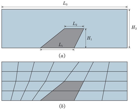
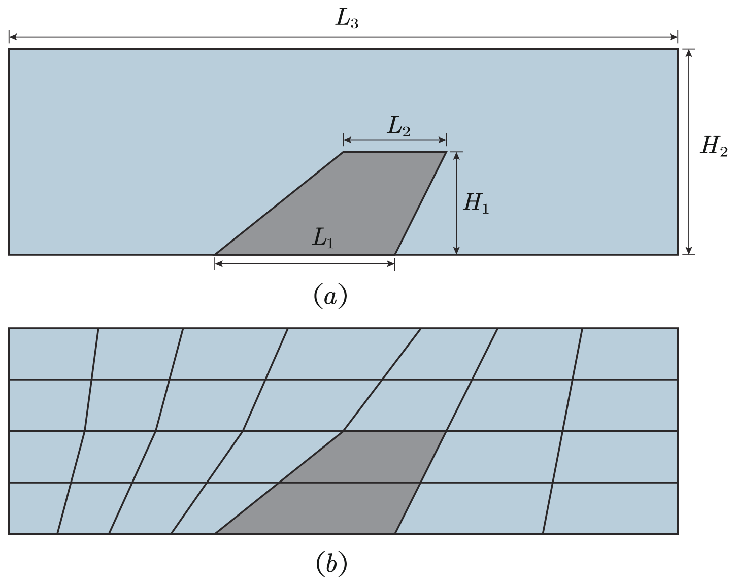
The second example considers a simplified tail structure subjected to external acoustic excitation, without considering mean flow or aerodynamic effects. This example is intended as a benchmark problem to evaluate the vibro-acoustic coupling performance of the proposed method. An acoustic medium with dimensions $L_3=13$ m and $H_2=4$ m surrounds the structure. The detailed geometric configuration is illustrated in Figure 9a. Here, the acoustic domain is indicated in blue, while the tail structure is shown in gray, with dimensions $L_1=3.5$ m, $L_2=2$ m, and $H_1=1.8$ m. The solid domain is made of TA15 titanium alloy, characterized by a Young’s modulus of $118 \mathrm{GPa}$, a density of $4450 \mathrm{kg}/{\mathrm{m}}^3$, and a Poisson’s ratio of $0.3$.

Figure 9. Schematic diagram of the tail structure: (a) Geometry of the tail. (b) Zonal domain of the tail.

Initially, the acoustic pressure is set to zero, and the tail structure is at rest. The time step used in the simulations is $\Delta t=0.001$, and the total simulation time is $T=0.05$. At $t=0$, a time-harmonic pressure load is applied on the left boundary of the acoustic domain, defined as

$$P\left(t\right)=5000\sin \left(\omega t\right) \mathrm{Pa},$$

where three excitation cases are considered, with $\omega =200\pi$, $\omega =300\pi$, and $\omega =400\pi$, corresponding to 100 Hz, 150 Hz and 200 Hz, respectively.

The purpose of this example is to investigate the frequency-dependent behavior of the vibro-acoustic system and to assess the performance of the proposed method under different excitation frequencies. A higher frequency results in a shorter wavelength, thereby imposing more stringent demands on spatial discretization.

The right boundary is treated as a non-reflecting condition to simulate an unbounded acoustic domain, while the bottom boundary of the tail structure is fully fixed. The computational domain is partitioned as shown in Figure 9b. In the COMSOL model, the tail structure contains 17,955 nodes, whereas the present method uses 10,302 nodes for discretization.

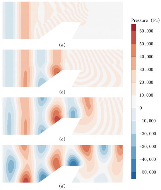
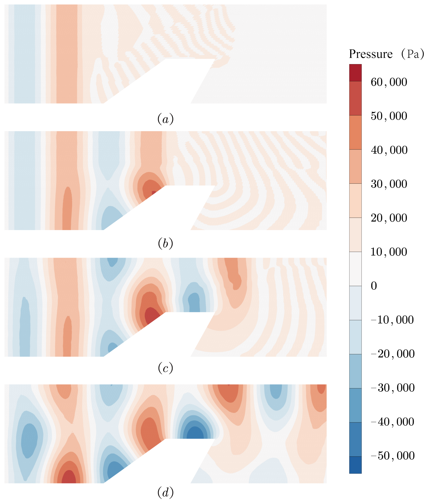
As shown in Figure 10, the evolution of acoustic pressure at different time instants is illustrated. At $t=0.01$ s, the wavefront is approximately planar. At $t=0.02$ s, when the wave reaches the leading edge of the tail structure, reflection phenomena begin to appear. At $t=0.03$ s, the wave has completely passed the trailing edge, and the acoustic field in front of the tail structure becomes stable without further significant changes.

Figure 10. Snapshots of acoustic pressure distributions at different time instants under $\omega =200\pi$: (a) $t=0.01$ s, (b) $t=0.02$ s, (c) $t=0.03$ s, (d) $t=0.05$ s.

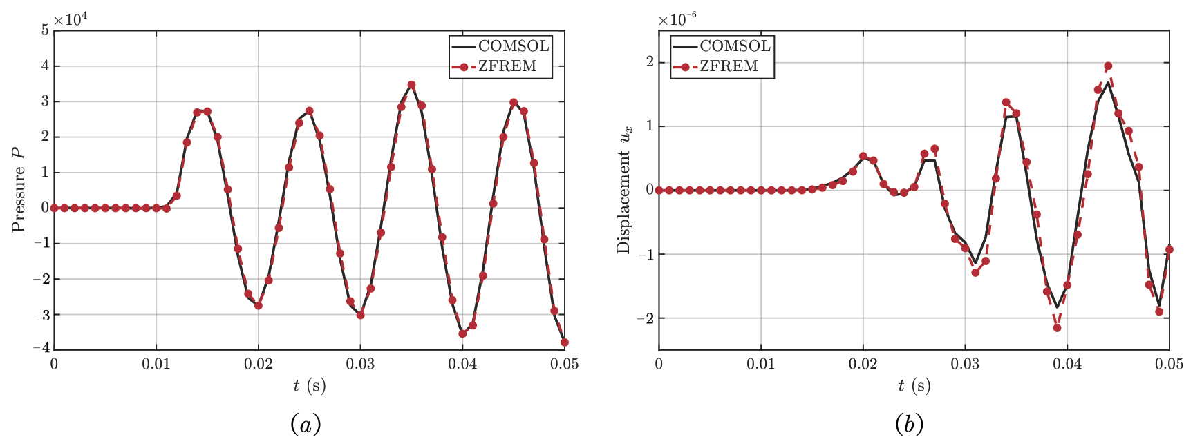
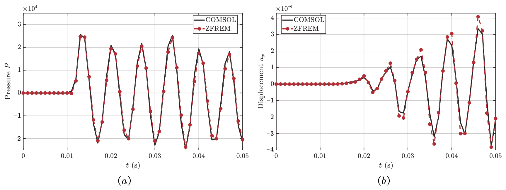
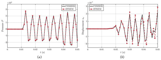
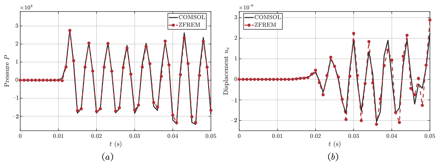
Figure 11, Figure 12 and Figure 13 present the comparisons of acoustic pressure and displacement responses under excitation frequencies of 100 Hz ($\omega =200\pi$), 150 Hz ($\omega =300\pi$), and 200 Hz ($\omega =400\pi$), respectively. As shown in these figures, good agreement between the proposed method and COMSOL is observed for all three excitation frequencies. To further quantify the agreement, a relative root-mean-square (RMS) error is introduced to measure the discrepancy between the present method (ZFREM) and COMSOL results.

$$\mathrm{RMS}=\sqrt{{\displaystyle \frac{{\sum }_{n=1}^N{\left(x_n^{\mathrm{ZFREM}}-x_n^{\mathrm{COMSOL}}\right)}^2}{{\sum }_{n=1}^N{\left(x_n^{\mathrm{COMSOL}}\right)}^2}}},$$

(31)

where $x_n$ denotes the response quantity (acoustic pressure or structural displacement) at the n-th time step, and N is the total number of sampled time steps. The relative RMS errors under different excitation frequencies are summarized in Table 1.

Figure 11. Comparisons of acoustic pressure and displacement responses obtained by the two methods under $\omega =200\pi$: (a) Acoustic pressure at node $(0, 0.9)$. (b) Displacement at node $(4.4, 1.62)$.

Figure 12. Comparisons of acoustic pressure and displacement responses obtained by the two methods under $\omega =300\pi$: (a) Acoustic pressure at node $(0, 0.9)$. (b) Displacement at node $(4.4, 1.62)$.

Figure 13. Comparisons of acoustic pressure and displacement responses obtained by the two methods under $\omega =400\pi$: (a) Acoustic pressure at node $(0, 0.9)$. (b) Displacement at node $(4.4, 1.62)$.

Table 1. Relative RMS errors of acoustic pressure and structural displacement under different excitation frequencies.

Frequency (Hz)	Pressure Error (%)	Displacement Error (%)
100	0.21	3.8
150	0.68	2.1
200	1.12	4.5

Based on this metric, the RMS errors of the acoustic pressure remain within 1.2% for all excitation frequencies, showing a slight increase with frequency. For the structural displacement, the RMS errors remain below 5%, indicating good overall agreement between the proposed method and COMSOL. With increasing frequency, the wavelength decreases, resulting in more rapid oscillations in both acoustic and structural responses. The proposed method maintains good agreement with the reference solutions under all considered excitation frequencies. Meanwhile, accurate results are obtained with the present discretization, demonstrating the capability of the proposed method to achieve reliable solutions.

5. Conclusions

A strong-form meshless framework has been presented for vibro-acoustic coupling analysis, combining Lagrange interpolation with a domain decomposition strategy. The method constructs local approximation spaces directly from nodal distributions, thereby eliminating mesh dependence and enabling fully differential discretization of both acoustic and structural governing equations, as well as their coupling interfaces. The Kronecker delta property of Lagrange interpolation allows boundary conditions to be imposed directly without additional constraints. A node-wise procedure is employed for the evaluation and assembly of spatial derivatives and system matrices, contributing to good numerical stability and implementation flexibility. Transient responses are computed using the Newmark-$\beta$ scheme, providing stable and accurate time integration. Numerical examples show good agreement with COMSOL results, demonstrating the accuracy and reliability of the proposed method. Overall, the present method provides a unified strong-form meshless framework for multi-physics vibro-acoustic problems, with advantages in handling complex geometries and multi-domain coupling.

References

- Sha, Y.; Zhao, W.; Tang, X.; Zhao, F. Acoustic and Vibration Response and Fatigue Life Analysis of Thin-Walled Connection Structures under Heat Flow Conditions. Aerospace 2024, 11, 287. [Google Scholar] [CrossRef] [Scilit]
- Rakow, J.F.; Waas, A.M. Thermal buckling of metal foam sandwich panels for convective thermal protection systems. J. Spacecr. Rockets 2005, 42, 832–844. [Google Scholar] [CrossRef] [Scilit]
- Rahman, T.; Jansen, E.L.; Tiso, P. A finite element-based perturbation method for nonlinear free vibration analysis of composite cylindrical shells. Int. J. Struct. Stab. Dyn. 2011, 11, 717–734. [Google Scholar] [CrossRef] [Scilit]
- Chen, Y.C.; Hwu, C. Boundary element method for vibration analysis of two-dimensional anisotropic elastic solids containing holes, cracks or interfaces. Eng. Anal. Bound. Elem. 2014, 40, 22–35. [Google Scholar] [CrossRef] [Scilit]
- Vaicaitis, R. Nonlinear response and sonic fatigue of national aerospace space plane surface panels. J. Aircr. 1994, 31, 10–18. [Google Scholar] [CrossRef] [Scilit]
- Zhang, G.J.; Yan, Y.J.; Li, P.B. Vibration test of structural noise and analysis of the aeroelastic coupling response of aircraft. Appl. Math. Mech. 2013, 34, 1157–1164. (In Chinese) [Google Scholar]
- Gao, X.W.; Wang, J.; Peng, H.F.; Yang, K. Advanced Boundary Element Method: Theory and Program; Science Press: Beijing, China, 2015. (In Chinese) [Google Scholar]
- Djojodihardjo, H. Vibro-acoustic analysis of the acoustic-structure interaction of flexible structure due to acoustic excitation. Acta Astronaut. 2015, 108, 129–145. [Google Scholar] [CrossRef] [Scilit]
- Zheng, Y.-T.; Gao, X.-W.; Peng, H.-F.; Xu, B.-B. The coupled method of multi-domain BEM and element differential method for solving multi-scale problems. Eng. Anal. Bound. Elem. 2020, 113, 145–155. [Google Scholar] [CrossRef] [Scilit]
- Zhu, Y.-M.; Gao, X.-W. Element Differential Method for Computational Acoustics in Time Domain. Int. J. Comput. Methods 2023, 20, 2250031. [Google Scholar]
- Afsar, H.; Peiwei, G.; Aldandani, M.; Akbar, Y.; Alam, M.M. Analyzing the acoustic wave propagation characteristics in discontinuous bifurcated waveguide. Chaos Solit. Fractals 2023, 172, 113499. [Google Scholar] [CrossRef] [Scilit]
- Beirão da Veiga, L.; Mora, D.; Rivera, G.; Rodríguez, R. A virtual element method for the acoustic vibration problem. Numer. Math. 2017, 136, 725–763. [Google Scholar]
- Gao, X.-W.; Gao, L.-F.; Zhang, Y.; Cui, M.; Lv, J. Free element collocation method: A new method combining advantages of finite element and mesh free methods. Comput. Struct. 2019, 215, 10–26. [Google Scholar] [CrossRef] [Scilit]
- Gao, X.-W.; Jiang, W.-W.; Xu, X.-B.; Liu, H.-Y.; Yang, K.; Lv, J.; Cui, M. Overview of advanced numerical methods classified by operation dimensions. Aerosp. Res. Commun. 2023, 1, 11522. [Google Scholar] [CrossRef] [Scilit]
- Wang, D.; Peng, H. A Hermite reproducing kernel Galerkin meshfree approach for buckling analysis of thin plates. Comput. Mech. 2013, 51, 1013–1029. [Google Scholar]
- Chen, P.; Wang, D.; Hou, S.; Chu, Y. Temporal stability and accuracy of least squares meshfree collocation method for transient heat conduction analysis. Comput. Mech. 2026, 77, 761–800. [Google Scholar]
- Jiang, W.-W.; Gao, X.-W.; Liu, H.-Y. Multi-physics zonal Galerkin free element method for static and dynamic responses of functionally graded magneto-electro-elastic structures. Compos. Struct. 2023, 321, 117217. [Google Scholar] [CrossRef] [Scilit]
- Xu, B.-B.; Gao, X.-W.; Cui, M. High precision simulation of thermal-mechanical problems in functionally graded materials by spectral element differential method. Compos. Struct. 2021, 270, 114084. [Google Scholar] [CrossRef] [Scilit]
- Liu, H.-Y.; Gao, X.-W.; Xu, B.-B. An implicit free element method for simulation of compressible flow. Comput. Fluids 2019, 192, 104276. [Google Scholar] [CrossRef] [Scilit]
- Liu, H.-Y.; Gao, X.-W.; Pan, T. Pressure-velocity coupled zonal free element method for fluid-solid conjugate heat transfer. Eng. Anal. Bound. Elem. 2023, 155, 251–263. [Google Scholar] [CrossRef] [Scilit]
- Gao, X.-W.; Liu, H.-Y.; Ruan, B. Discontinuous zone free element method with variable condensation and applications in thermal-stress analysis of functionally graded material structures with cracks. Comput. Struct. 2021, 243, 106411. [Google Scholar] [CrossRef] [Scilit]
- Lv, J.; Song, C.; Gao, X.-W. Element differential method for free and forced vibration analysis for solids. Int. J. Mech. Sci. 2019, 151, 828–841. [Google Scholar] [CrossRef] [Scilit]
Disclaimer/Publisher’s Note: The statements, opinions and data contained in all publications are solely those of the individual author(s) and contributor(s) and not of MDPI and/or the editor(s). MDPI and/or the editor(s) disclaim responsibility for any injury to people or property resulting from any ideas, methods, instructions or products referred to in the content. |
© 2026 by the authors. Licensee MDPI, Basel, Switzerland. This article is an open access article distributed under the terms and conditions of the Creative Commons Attribution (CC BY) license.