A Composite Control Strategy for Aircraft Anti-Skid Braking Systems Based on Gaussian Quantum Particle Swarm Optimization

Abstract

The performance of the aircraft anti-skid braking system is critical to the ground operational safety of an aircraft. Conventional Pressure Bias Modulation (PBM) can suffer from deep skidding under low runway friction coefficients or low aircraft speeds. To address these issues, a composite control strategy based on Gaussian Quantum Particle Swarm Optimization (GQPSO) is proposed. This strategy employs the GQPSO algorithm for offline Proportional–Integral–Derivative (PID) parameter optimization, followed by real-time adaptive scheduling through a lookup table to accommodate varying speed domains and runway conditions. Simultaneously, by integrating the main-wheel dynamics model and friction characteristics, a runway identification function based on a Back Propagation Neural Network (BPNN) is designed to provide runway status information. The stability of the controller is verified via phase-plane analysis and Monte Carlo simulation. Subsequently, comparative Hardware-in-the-Loop (HIL) tests are conducted among PBM, PSO-PID, and the proposed GQPSO-PID controller under various runway conditions. The experimental results demonstrate that this composite controller can adapt to different speed domains and runway conditions, stably track the target slip ratio, effectively suppress skidding, and significantly improve braking efficiency, as well as exhibiting excellent robustness and control performance.

1. Introduction

The aircraft anti-skid braking system (ABS) is a critical subsystem that ensures ground safety by enabling efficient braking to shorten the taxiing distance while preventing wheel skidding or lock-up [1,2,3]. Data indicate that approximately 50% of global aviation accidents occur during the taxiing phase [4]. Although modern aircraft braking systems include auxiliary devices such as spoilers, thrust reversers, and deceleration parachutes, the use of these devices is subject to various operational limitations [5,6,7,8]. In contrast, wheels, as the only braking mechanism operable across the full speed range and all weather conditions, have a braking performance that directly impacts the aircraft’s taxiing safety [9]. If the anti-skid system fails, the wheels are prone to deep skidding or even lock-up, which not only reduces braking efficiency but also significantly increases the risk of tire blowouts, posing a serious threat to taxiing safety [10,11]. Therefore, developing efficient and reliable anti-skid braking controllers remains a key research focus in the modern aviation industry.

The friction provided by the runway to the wheels is influenced by a combination of runway conditions and wheel motion states. Consequently, the core of designing an aircraft anti-skid braking system lies in controlling the braking pressure to maximize the utilization of runway friction while preventing wheel lock-up, thereby reducing the taxiing distance. Currently, traditional Pressure Bias Modulation (PBM) is widely used in existing aircraft anti-skid braking systems due to advantages such as strong robustness, high reliability, and simple implementation [12,13]. PBM is an improved form of Proportional–Integral–Derivative (PID) control, where the PBM module replaces the integral module of PID, offering strong runway adaptability and reliability. However, this control method is prone to inducing deep wheel skidding on runways with low friction coefficients or at low speeds, leading to poor braking efficiency [14,15]. The root cause lies in the uncertainties, strong nonlinearities, and real-time requirements of aircraft anti-skid braking systems, which pose significant challenges to controller design [16,17,18]. To address these issues, researchers have proposed various new anti-skid control strategies, such as Model Predictive Control (MPC) [19,20], Sliding Mode Control (SMC) [21,22], Fuzzy Control (FC) [23,24], and Artificial Neural Network Control (ANNC) [25,26]. However, SMC struggles to avoid inherent chattering issues, which may affect braking stability [27,28]; the control rules of FC heavily rely on expert prior knowledge [29,30]; MPC requires accurate system models and imposes high real-time computational loads [31,32]; meanwhile, ANNC demands extensive experimental data for model training, with complex learning processes and generalization capabilities limited by data quality [33,34,35].

Given the advantages of PID control, such as simple structure and ease of engineering implementation, along with the rise of intelligent algorithms, various intelligent algorithms are often used for self-tuning PID control parameters [36,37]. Compared with traditional PID control, PID control combined with intelligent algorithms can achieve better control effects and higher efficiency [38]. Among them, the Particle Swarm Optimization (PSO) algorithm, known for its fast convergence, few adjustable parameters, and strong global search capability, has been gradually introduced into the design of aircraft anti-skid braking controllers. In this regard, Fengrui Xu et al. proposed an active disturbance rejection anti-skid control algorithm based on PSO, which optimizes the parameters of active disturbance rejection control using PSO, enabling the system to operate within a stable region without deep skidding [39]. Jennan N et al. designed an anti-skid control method based on PSO, optimizing the additive term in the reaching law with PSO, significantly improving braking performance [40]. Lei Li et al. proposed an aircraft braking control algorithm based on an improved PSO algorithm, identifying key parameters for optimal control through PSO and optimizing both braking distance and anti-skid performance [41]. Compared to the traditional PSO algorithm, the Gaussian Quantum Particle Swarm Optimization (GQPSO) algorithm offers faster convergence and more robust global search capabilities, and it has been widely used in fields such as new energy, biology, and medicine [42,43,44]. However, research on the application of GQPSO in aircraft anti-skid braking control remains relatively scarce.

Beyond intelligent PID optimization, recent studies have also examined aircraft anti-skid braking from the perspectives of runway-friction estimation, gain-scheduled controller design, stability verification, and implementation-oriented validation [45,46,47]. These studies indicate that these aspects should be considered together in aircraft anti-skid braking design.

To address the above research gaps, this paper develops an integrated Hardware-in-the-Loop (HIL)-validated control framework that combines GQPSO-based PID parameter scheduling, runway identification, and stability screening. In this framework, a back-propagation neural network (BPNN) runway identification module based on main-wheel dynamics is designed to provide the target slip-ratio reference. GQPSO is used to generate offline PID gain lookup tables, and the scheduled gains are applied online according to aircraft speed, real-time slip ratio, and the identified target slip ratio. Phase-plane analysis and Monte Carlo simulation (MCS) are used as a stability-screening step before HIL testing. Finally, the proposed controller is compared with PBM and PSO-PID under dry–wet and dry–ice mixed runway conditions to evaluate its slip-ratio tracking, recovery after runway-friction changes, and braking performance.

(1)

Proposing a runway status identification method based on the BPNN and the Magic Formula (MF) model, which can effectively identify runway status information, thereby providing the controller with a target slip ratio for efficient braking and laying the foundation for braking efficiency optimization;

(2)

Developing a GQPSO-based offline PID parameter scheduling method, in which the optimized gains are implemented through lookup tables to achieve accurate tracking of the target slip ratio and enhance the controller’s adaptability to complex operating conditions;

(3)

Establishing a validation procedure that combines phase-plane analysis, MCS-based stability screening, and HIL tests under abrupt runway-friction changes, thereby linking parameter optimization, local stability constraints, and braking-performance evaluation.

The remainder of this paper is organized as follows: Section 2 establishes the dynamic model of the aircraft braking system. Section 3 develops a composite aircraft anti-skid braking controller based on GQPSO. Section 4 validates the proposed controller through HIL experiments. Section 5 contains the conclusions and suggestions for future work.

2. Modeling of Aircraft Braking System

2.1. Dynamic Model of the Airframe

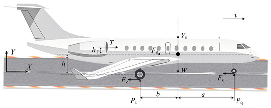
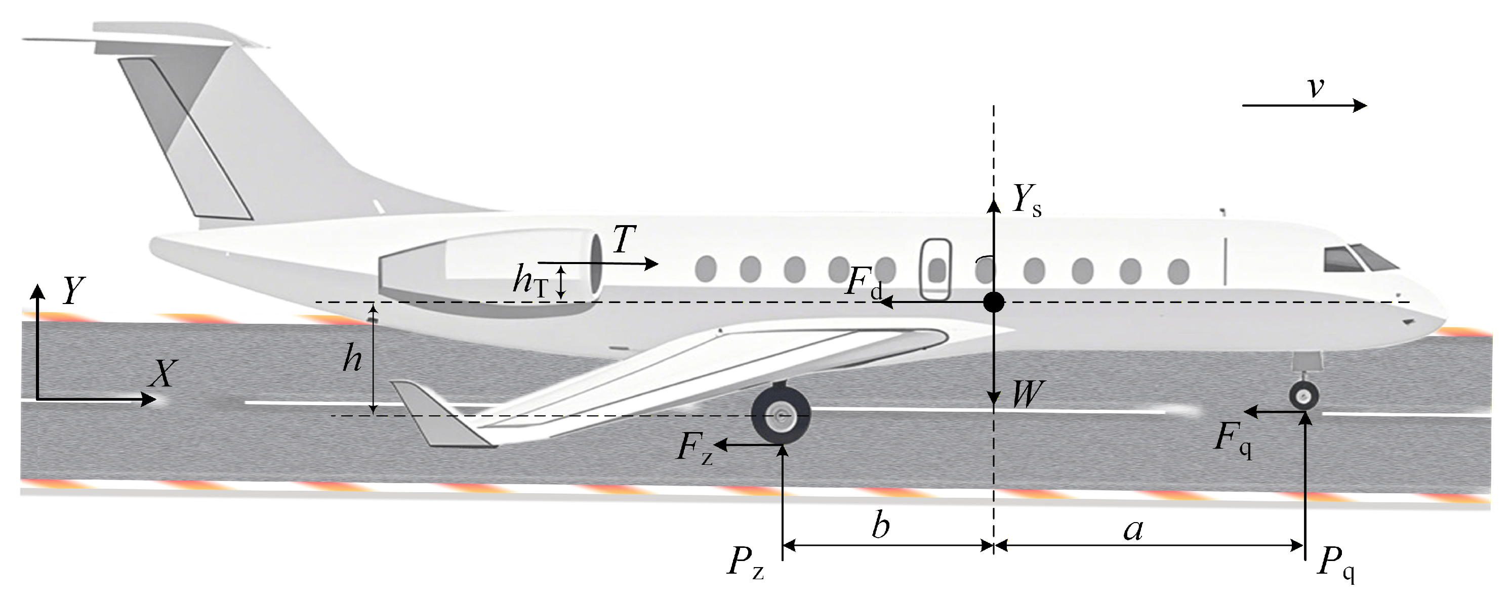
During the aircraft landing taxiing process, its motion state is influenced by various complex factors. To simplify the system analysis and modeling, the following assumptions are made in this paper: it is assumed that the aircraft motion is rigid-body motion always along the runway direction, while ignoring lateral disturbances such as crosswinds, landing gear shimmy, and nose wheel steering. Based on these simplified conditions, the dynamics model of the airframe during the landing taxiing process is established, and its force analysis is shown in Figure 1. The kinetic equilibrium equation for aircraft taxiing is shown in Equation (1).

$$\left\{\begin{array}{l}{\displaystyle \sum F_x}=T-F_d-F_z-F_q-{\displaystyle \frac{W}{\mathrm{g}}}\cdot \dot{v}=0\hfill \\ {\displaystyle \sum F_y}=Y_s+P_z+P_{\mathrm{q}}-W=0\hfill \\ {\displaystyle \sum M}=P_q\cdot a-P_z\cdot b-(F_z+F_q)\cdot h-T\cdot h_T=0\hfill \end{array}\right.$$

(1)

where $W$ is the aircraft landing weight, $g$ is the gravitational acceleration, $T$ is the engine idle thrust, $\dot{v}$ is the acceleration of the airframe along the longitudinal axis, $Y_{\mathrm{s}}$ is the aircraft lift force, $F_{\mathrm{d}}$ is the air resistance, $P_{\mathrm{z}}$ is the load on the main gear, $P_{\mathrm{q}}$ is the load on the nose gear, $F_{\mathrm{z}}$ is the ground friction force on all the main wheels, $F_{\mathrm{z}}=P_{\mathrm{z}}·\mu$, $\mu$ is the friction coefficient of the main wheels, $F_{\mathrm{q}}$ is the ground friction force on the nose wheel, $F_{\mathrm{q}}=P_{\mathrm{q}}·{\mu }_{\mathrm{gd}}$, ${\mu }_{\mathrm{gd}}$ is the rolling friction coefficient of the nose wheel, $a$ and $b$ represent the longitudinal distances from the center of gravity to the nose and main landing gear centers, respectively, $h_{\mathrm{T}}$ is the distance from the aircraft’s center of gravity to the engine thrust line, and $h$ is the distance from the aircraft’s center of gravity to the wheel center.

Figure 1. Force analysis diagram of the aircraft during taxiing.

Under the assumption that the atmosphere is an ideal fluid, the lift force and aerodynamic drag acting on the airframe can be calculated using the established aerodynamic model, as shown in the Equation (2).

$$\left\{\begin{array}{l}{Y}_{\mathrm{s}}={\displaystyle \frac{1}{2}}\cdot \rho \cdot v^2\cdot S\cdot C_{\mathrm{Y}}\hfill \\ F_{\mathrm{d}}={\displaystyle \frac{1}{2}}\cdot \rho \cdot v^2\cdot S\cdot C_{\mathrm{X}}\hfill \end{array}\right.$$

(2)

where $\mathsf{\rho }$ is the air density at the landing airport, $S$ is the wing windward area, and $C_{\mathrm{X}}$ and $C_{\mathrm{Y}}$ are the aircraft’s aerodynamic drag and lift coefficients, respectively.

During the aircraft landing taxiing process, the engine needs to maintain low-power operation, thus resulting in some residual thrust. Considering the influence of engine residual thrust, this paper establishes an engine model to reflect the variation pattern of thrust, as shown in the Equation (3).

$$T=K_{\mathrm{m}}\cdot v$$

(3)

where $K_{\mathrm{m}}$ is the engine residual thrust coefficient.

Combining Equations (1)–(3), the acceleration of the aircraft along the X-axis is obtained as:

$$\begin{array}{ll}\dot{v}& ={\displaystyle \frac{g\cdot T}{W}}-{\displaystyle \frac{g\cdot \rho \cdot C_{\mathrm{X}}\cdot S\cdot v^2}{2W}}-{\displaystyle \frac{g\cdot \mu \cdot [(W-Y_{\mathrm{s}})\cdot (a-{\mu }_{\mathrm{gd}}\cdot h)-T\cdot h_{\mathrm{T}}]}{W\cdot [a+b+(\mu -{\mu }_{\mathrm{gd}})\cdot h]}}\\ & -{\displaystyle \frac{g\cdot {\mu }_{\mathrm{gd}}\cdot [(W-Y_{\mathrm{s}})\cdot b+T\cdot h_{\mathrm{T}}]}{W\cdot [a+b+(\mu -{\mu }_{\mathrm{gd}})\cdot h]}}\end{array}$$

(4)

2.2. Dynamics Model of the Wheel

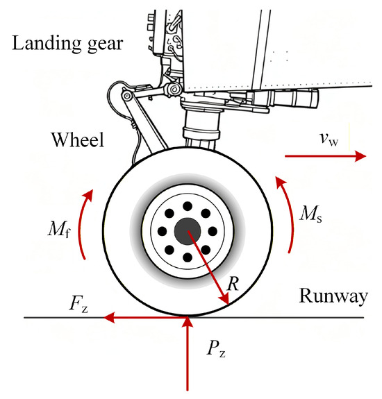
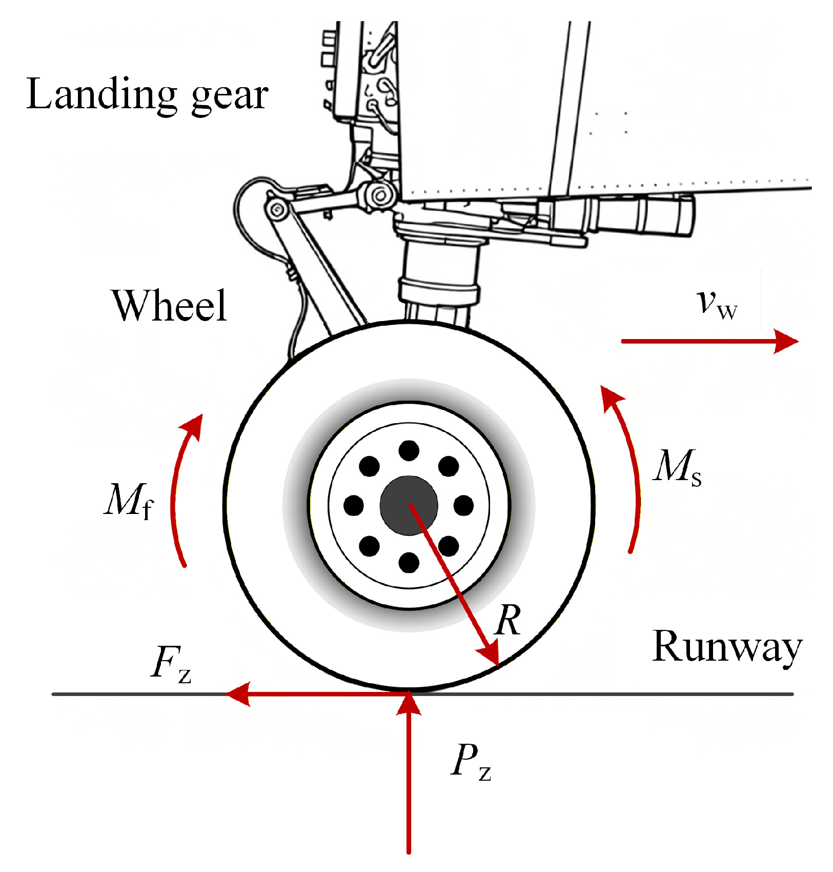
The aircraft wheel braking is primarily achieved by the main wheels. The force analysis diagram for the main wheel motion is shown in Figure 2. The main wheel rotates under the combined action of the braking torque and the ground reaction torque. Accordingly, the dynamics model of the wheel can be established, as shown in the Equation (5).

$$\left\{\begin{array}{l}{v}_{\mathrm{w}}=\omega \cdot R\hfill \\ M_f=F_{\mathrm{z}}\cdot R\hfill \\ \dot{\omega }={\displaystyle \frac{M_{\mathrm{f}}-M_{\mathrm{s}}}{J_{\mathrm{g}}}}\hfill \end{array}\right.$$

(5)

where $v_{\mathrm{w}}$ is the speed of the main wheel, $\omega$ is the angular velocity of the main wheel, $R$ is the rolling radius of the wheel, $M_{\mathrm{f}}$ is the ground friction torque acting on the main wheel, $M_{\mathrm{s}}$ is the braking torque acting on the main wheel, and $J_{\mathrm{g}}$ is the rotational inertia of the wheel.

Figure 2. Force analysis diagram of the main wheel motion.

The friction coefficient between the runway and the wheel is difficult to measure directly. Compared to other descriptive methods, the MF model has better uniformity, practicality, and higher fitting accuracy, so it is often used to indirectly estimate the runway friction coefficient [48,49]. In summary, the friction model between the wheel and the runway can be established using the MF model, as shown in the Equation (6).

$$\mu =D\cdot \sin [C\cdot \arctan (B\cdot \sigma )]$$

(6)

where $B$ is the stiffness factor, $C$ is the shape factor, and $D$ is the peak factor.

During aircraft taxiing, under the combined action of the braking torque and the ground friction torque, the wheel is usually in a state of partial sliding and partial rolling. When the braking torque exceeds the ground friction torque, the wheel locks up, entering a state of pure sliding. Typically, the wheel’s motion state is described by the slip ratio, as shown in the Equation (7).

$$\sigma ={\displaystyle \frac{v-v_{\mathrm{w}}}{v}}$$

(7)

When the slip ratio is close to 1, the wheel is considered locked; when the slip ratio is close to 0, the wheel is in a state of pure rolling.

The system equation is defined as:

$$\left\{\begin{array}{c}{x}_1=\sigma \\ x_2=\dot{\sigma }\end{array}\right.$$

(8)

3. Controller Design

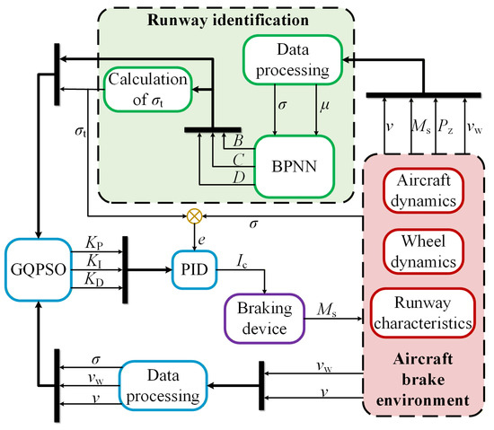
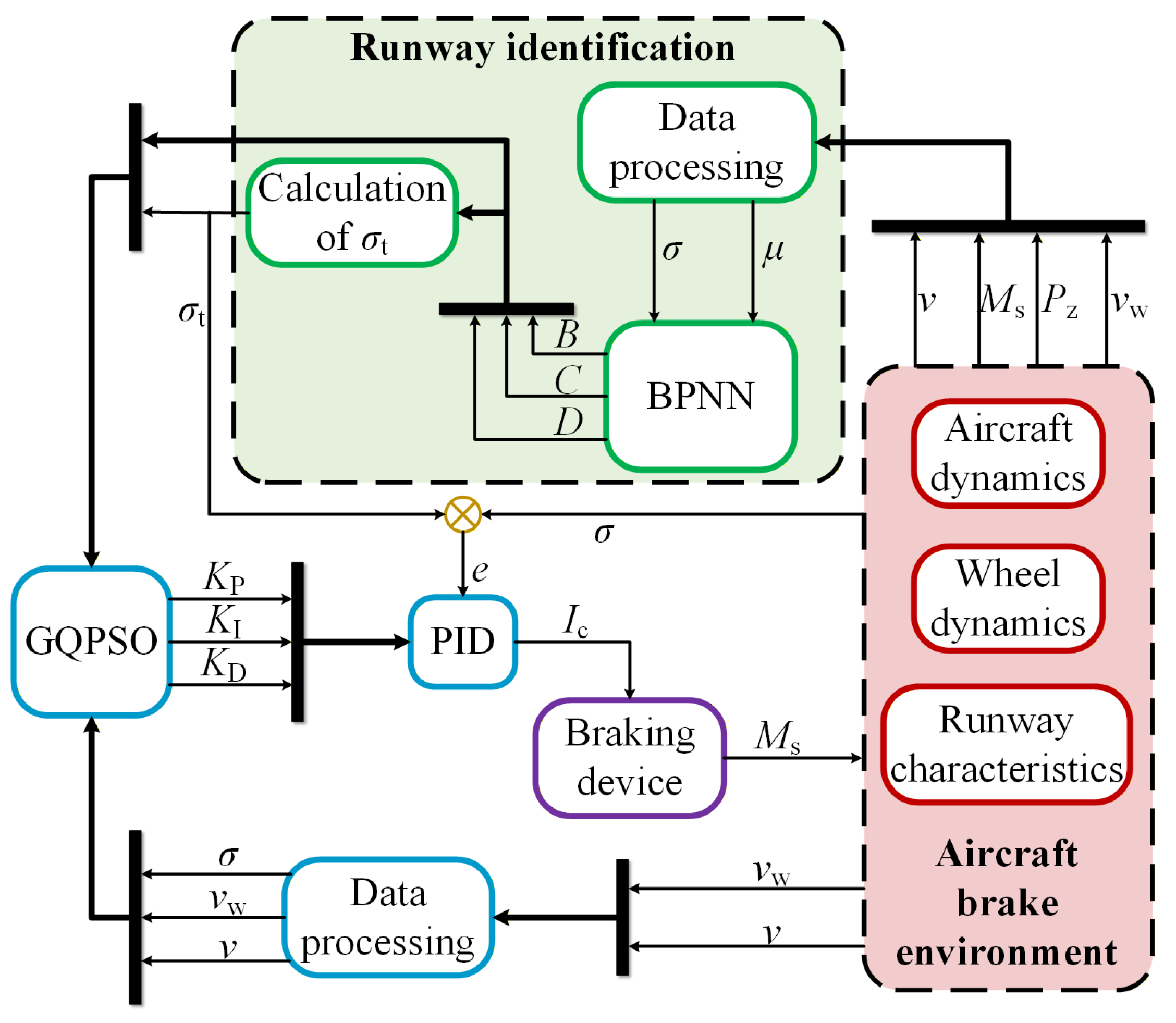
To enhance the control performance and braking efficiency of the PID controller across the full speed range and under all runway conditions, this paper designs a controller framework as shown in Figure 3. The core components of this framework include a runway status identification module based on BPNN, a PID controller based on GQPSO, and a priori stability constraint settings. Among these, the runway status identification module takes the wheel speed, aircraft speed, braking torque, and vertical load as inputs and estimates the runway status information and target slip ratio via the BPNN. The GQPSO-based PID controller adopts a parameter scheduling mechanism, where the PID parameters are pre-calculated offline using the GQPSO algorithm and stored in a lookup table. During operation, the controller retrieves the optimal parameters based on the real-time identified runway state and aircraft speed. Taking the slip ratio error as input, the controller then commands the braking device to output an appropriate braking torque, thereby achieving precise tracking of the target slip ratio. In the stability analysis phase, the criterion for determining the type of singular points is first analyzed using the phase-plane method. Subsequently, the distribution of stable singular points within the PID controller parameter space is statistically analyzed using MCS, ultimately validating the system’s stability. The following sections will elaborate in detail on the BPNN-based runway status identification module, the GQPSO-based PID controller, and the stability analysis process.

Figure 3. Overall framework of the controller.

3.1. Runway Status Identification Based on BPNN

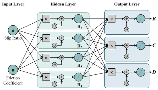
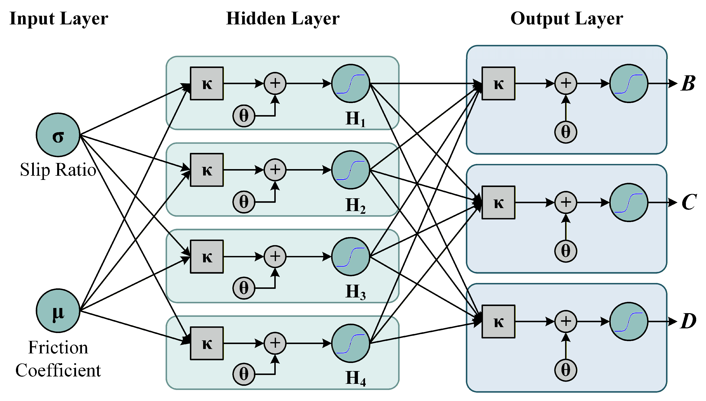
The main wheels directly participate in the conversion of braking energy and produce significant slip during deceleration, making their dynamic response highly sensitive to runway conditions. From Equations (5) and (6), it is known that $f(\dot{\omega },{ P}_{\mathrm{z}}) = f\left(B, C, D, \sigma \right)$. However, due to the interference of the braking torque, the raw angular acceleration cannot accurately reflect the runway status. Therefore, a data pre-processing stage is implemented prior to the neural network. In this stage, the angular acceleration is decoupled based on the braking torque. Derived from Equation (5), the decoupled equivalent free-rolling angular acceleration can be obtained as ${\dot{\omega }}_{\mathrm{eq}} = \dot{\omega }+M_{\mathrm{s}}/J_{\mathrm{g}}$, which is subsequently utilized to deduce the friction coefficient $\mu$. Consequently, a BPNN identification module can be established with the friction coefficient $\mu$ and slip ratio $\sigma$ as inputs and runway status parameters as outputs. Based on these output runway status parameters, a solver subsequently computes the optimal slip ratio that maximizes the friction coefficient via the MF model. Finally, this optimal slip ratio is designated as the target slip ratio for the anti-skid controller. The structure of the backpropagation neural network is shown in Figure 4.

Figure 4. Schematic diagram of the back propagation neural network.

The basic computational logic of the BPNN involves, over multiple iterations, repeatedly calculating the output results of the hidden and output layers, while continuously updating the weights and bias coefficients of the hidden and output layers based on error feedback, until the training termination condition is met. The operational steps of the BPNN are detailed below.

The input vector X and output vector Y of the BPNN are, respectively:

$$\left\{\begin{array}{l}X=[\mu ,\sigma ]=[X_1,X_2]\hfill \\ Y=[B,C,D]=[Y_1,Y_2,Y_3]\hfill \end{array}\right.$$

(9)

The activation function for the hidden layer $f_{\mathrm{h}}$ and the output layer $f_{\mathrm{o}}$ are, respectively:

$$\left\{\begin{array}{l}{f}_{\mathrm{h}}(x)={\displaystyle \frac{1-e^{-x}}{1+e^{-x}}}\hfill \\ f_{\mathrm{o}}(x)={\displaystyle \frac{1}{1+e^{-x}}}\hfill \end{array}\right.$$

(10)

The input value $s_{\mathrm{j}}$ and output value $h_{\mathrm{j}}$ for the j-th node (j = 1, 2, , nh) in the hidden layer are, respectively:

$$\left\{\begin{array}{l}{s}_{\mathrm{j}}={\displaystyle \sum _{\mathrm{i}=1}^{\mathrm{n}}({\kappa }_{\mathrm{ij}}\cdot X_{\mathrm{i}})+{\theta }_{\mathrm{j}}}\hfill \\ h_{\mathrm{j}}=f_{\mathrm{h}}(s_{\mathrm{j}})\hfill \end{array}\right.$$

(11)

where ${\kappa }_{\mathrm{ij}}$ is the weight from the i-th node in the input layer to the j-th node in the hidden layer, and ${\theta }_{\mathrm{j}}$ is the bias of the j-th node in the hidden layer.

The input value $l_{\mathrm{k}}$ and output value $Y_{\mathrm{k}}$ for the k-th node (k = 1, 2, …, p) in the output layer are, respectively:

$$\left\{\begin{array}{l}{l}_{\mathrm{k}}={\displaystyle \sum _{\mathrm{j}=1}^{\mathrm{nh}}({\kappa }_{\mathrm{jk}}\cdot h_{\mathrm{j}})+{\theta }_{\mathrm{k}}}\hfill \\ Y_{\mathrm{k}}=f_{\mathrm{o}}(l_{\mathrm{k}})\hfill \end{array}\right.$$

(12)

where ${\kappa }_{\mathrm{jk}}$ is the weight from the j-th node in the hidden layer to the k-th node in the output layer, and ${\theta }_{\mathrm{k}}$ is the bias of the k-th node in the output layer.

The mean square error E for the sample is:

$$E={\displaystyle \frac{1}{2}}{\displaystyle \sum _{\mathrm{k}=1}^{\mathrm{p}}{(Y_{\mathrm{k}}-t_{\mathrm{k}})}^2}$$

(13)

where $t_{\mathrm{k}}$ is the sample label corresponding to the k-th node in the output layer.

The residual error ${\delta }_{\mathrm{k}}$ for the output layer and the residual error ${\delta }_{\mathrm{j}}$ for the hidden layer are, respectively:

$$\left\{\begin{array}{l}{\delta }_{\mathrm{k}}=Y_{\mathrm{k}}\cdot (t_{\mathrm{k}}-Y_{\mathrm{k}})\cdot (1-Y_{\mathrm{k}})\hfill \\ {\delta }_j={\displaystyle \frac{1-{h_{\mathrm{j}}}^2}{2}}[{\displaystyle \sum _{\mathrm{k}=1}^{\mathrm{p}}({\delta }_{\mathrm{k}}\cdot {\kappa }_{\mathrm{jk}})}]\hfill \end{array}\right.$$

(14)

The updated weight ${\stackrel{\mathrm{~}}{\kappa }}_{\mathrm{ij}}$ between the input and hidden layers and the updated weight ${\stackrel{\mathrm{~}}{\kappa }}_{\mathrm{jk}}$ between the hidden and output layers are, respectively:

$$\left\{\begin{array}{l}{\tilde{\kappa }}_{\mathrm{ij}}={\kappa }_{\mathrm{ij}}+\eta \cdot h_{\mathrm{j}}\cdot {\delta }_{\mathrm{k}}\hfill \\ {\tilde{\kappa }}_{\mathrm{jk}}={\kappa }_{\mathrm{jk}}+\eta \cdot X_{\mathrm{j}}\cdot {\delta }_{\mathrm{j}}\hfill \end{array}\right.$$

(15)

where η is the learning rate. A larger learning rate reduces the number of cycles required to meet the training error; however, an excessively large learning rate will cause obvious network oscillations. Generally, the optimal range for the learning rate is 0.1 to 0.3 [50].

The updated hidden layer bias ${\stackrel{\mathrm{~}}{\theta }}_{\mathrm{j}}$ and output layer bias ${\tilde{\theta }}_{\mathrm{k}}$ are, respectively:

$$\left\{\begin{array}{l}{\tilde{\theta }}_{\mathrm{k}}={\theta }_{\mathrm{k}}+\eta \cdot {\delta }_{\mathrm{k}}\hfill \\ {\tilde{\theta }}_{\mathrm{j}}={\theta }_{\mathrm{j}}+\eta \cdot {\delta }_{\mathrm{j}}\hfill \end{array}\right.$$

(16)

Subsequently, the calculation steps from Equation (11) to Equation (16) are repeated for the training sample data until the global average error falls below a preset threshold or the maximum number of iterations is reached, at which point the training process terminates.

To ensure the deterministic convergence of the network training, a high-dimensional mechanistic database is constructed. It comprises 935,362 independent data groups. The dataset generation is based on the physical mechanism model of the MF. Multi-dimensional grid loops with variable step sizes are executed within the strict boundaries of the characteristic parameters. These parameter ranges are configured as follows: stiffness factor $B \in [10.0326, 12.2198]$, shape factor $C \in [1.5344, 2.0875]$, and curvature factor $D \in [0.18, 0.8]$. Concurrently, a full-spectrum parametric sweep was conducted over the slip ratio domain $\sigma \in [0, 1]$ with a fine step of 0.01.

However, the dataset originates from deterministic numerical simulation grid sampling. Therefore, high correlations inevitably exist among the samples. To eliminate the impact of this high correlation on network generalization, a chaotic mapping algorithm is introduced. This algorithm performs nonlinear pseudo-random partitioning to decouple the database. The discrete iterative state equation of the chaotic system is defined as follows:

$$l_{\mathrm{k}+1}=\xi \cdot l_{\mathrm{k}}\cdot (1-l_{\mathrm{k}})$$

(17)

where $l_{\mathrm{k}}$ represents the chaotic state variable, $l_{\mathrm{k}} \in (0,1)$, and $\xi$ is the chaotic coefficient, $\xi \in (0,4]$. A larger chaotic coefficient indicates a higher degree of chaotic intensity. Subsequently, the total sample pool is separated into a training set (70%), a mutually exclusive validation set (15%), and an independent testing set (15%) based on this method. Under this partitioning mechanism, the training samples are used to drive the gradient calculations for error backpropagation. In contrast, the testing samples are used to verify the generalization capability after the training ends. This approach successfully eliminates the artificial inflation of the goodness-of-fit.

To eliminate the impact of dimensional disparities among different physical variables, a min–max normalization procedure is applied to the dataset prior to learning. All input and output features are linearly mapped into a bounded interval of [0.1, 0.9].

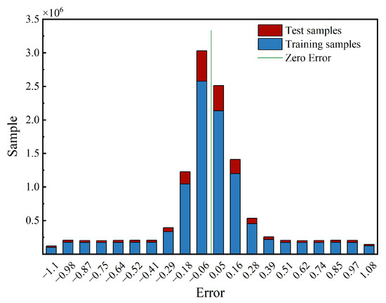
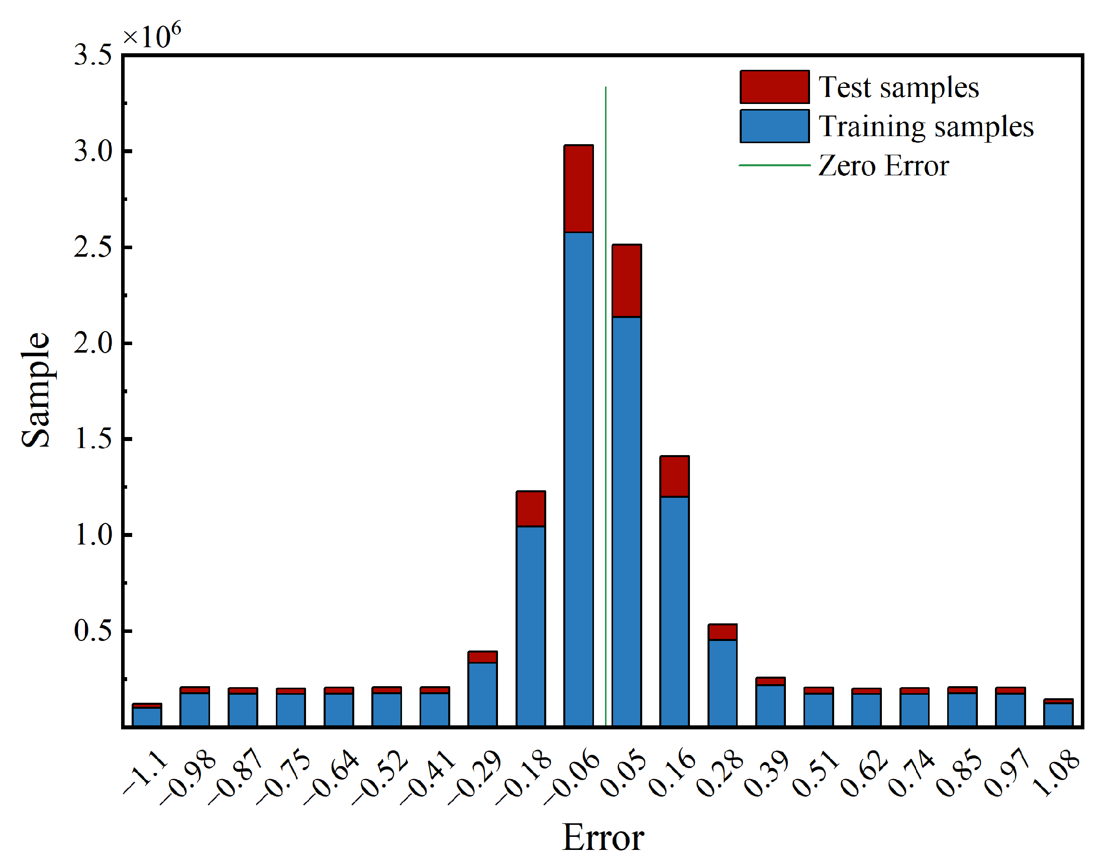
In this study, the termination conditions for the BPNN training are set as follows: reaching a maximum of 1000 iterations or the gradient dropping below 1.0 × 10⁻⁷. The training results showed that after 415 iterations of the sample data, the gradient dropped to 1.12 × 10⁻⁸ (less than 1.0 × 10⁻⁷), and the training stopped accordingly. Validation shows that the fitting degree of the trained neural network reaches 0.9976. Its error distribution is shown in Figure 5. As can be seen from the figure, the error values of most samples are concentrated near zero, and there are very few samples that are obvious outliers. This indicates that the neural network possesses high fitting accuracy and good generalization capability, making it suitable for runway status identification.

Figure 5. Neural network error distribution.

As known from the MF model, the relationship between the runway friction coefficient and the slip ratio exhibits a “first increase then decrease” characteristic: in the first stage, the friction coefficient increases with the slip ratio, reaches a peak, and then decreases with further increase in slip ratio. However, even when the wheel locks, its friction coefficient remains higher than in pure rolling. Therefore, when the derivative of the runway friction coefficient with respect to the slip ratio is zero, the friction coefficient reaches its peak. If this slip ratio can be maintained, the maximum braking efficiency can be achieved.

Combining with Equation (5), the slip ratio ${\sigma }_{\mu \max }$ corresponding to the peak friction coefficient can be calculated as:

$${\sigma }_{\mu \max }={\displaystyle \frac{\tan (\frac{\pi }{2C})}{B}}$$

(18)

However, if the slip ratio corresponding to the maximum friction coefficient is directly set as the target slip ratio, the actual slip ratio can easily fall into the descending segment of the friction curve, causing frequent wheel skidding and significantly reducing the stability of the anti-skid system [51]. Therefore, it is necessary to shift the target slip ratio towards the ascending segment of the friction curve by introducing a bias amount ε for correction. The final target slip ratio ${\sigma }_{\mathrm{t}}$ is:

$${\sigma }_{\mathrm{t}}={\sigma }_{\mu \max }+\epsilon$$

(19)

3.2. PID Controller Based on GQPSO

To improve the robustness and adaptability of PID control, this study uses the GQPSO algorithm to optimize the PID control parameters. The traditional PID controller takes the error between the actual slip ratio and the target slip ratio as the control object, outputting a braking torque control signal to track the target slip ratio. Its braking torque control signal $M_{\mathrm{sc}0}$ is:

$$M_{\mathrm{sc}0}=K_{\mathrm{p}}\cdot e+K_{\mathrm{i}}\cdot {\displaystyle \int e} \mathrm{d}t+K_{\mathrm{d}}\cdot \dot{e}$$

(20)

where $e$ is the error between the actual slip ratio and the target slip ratio, $e ={ \sigma }_{\mathrm{t}}-\sigma$, $K_{\mathrm{p}}$ is the proportional coefficient, $K_{\mathrm{i}}$ is the integral coefficient, and $K_{\mathrm{d}}$ is the derivative coefficient.

The Quantum Particle Swarm Optimization (QPSO) algorithm introduces quantum mechanics concepts based on the traditional (PSO) algorithm. It characterizes the particle swarm state using a wave function $\psi \left(x, t\right)$, replacing the description of particle position and velocity in traditional algorithms, making the particle search process more flexible. The GQPSO algorithm is a further improvement on QPSO, replacing the original uniform random numbers with a Gaussian probability distribution mutation operator. This ensures the generation of numerous small-amplitude steps near the current position for local fine-tuning, while also allowing, with a small probability, the generation of larger-amplitude steps to escape local optima [52].

The basic computational logic of GQPSO is that, over multiple iterations, particle positions are continuously updated based on the fitness function and historical search results, searching for the particle position corresponding to the optimal fitness value until the maximum number of iterations is reached. The operational steps of the GQPSO algorithm are detailed below.

The initial position of the particles is:

$$x_{\mathrm{i},\mathrm{d}}(0)~U(l{b}_{\mathrm{d}},u{b}_{\mathrm{d}})$$

(21)

where i is the population size, i = 1, 2, …, m; d is the optimization dimension, d = 1, 2, …, n; $U({lb}_{\mathrm{d}},{ub}_{\mathrm{d}})$ is the uniform distribution in the d-th dimension search space; and ${lb}_{\mathrm{d}}$ and ${ub}_{\mathrm{d}}$ are the lower and upper bounds of the d-th dimension, respectively.

The initial individual best pbest value is:

$$pbes{t}_{\mathrm{i},\mathrm{d}}(0)=x_{\mathrm{i},\mathrm{d}}(0)$$

(22)

The initial global best gbest value is:

$$gbest(0)=\arg {\min }_{\mathrm{i}=1..\mathrm{m}}f(pbes{t}_{\mathrm{i}}(0))$$

(23)

The optimal result should make the actual slip ratio closer to the target slip ratio, so the fitness function f is:

$$f=\min (w_1\left|({\sigma }_{\mathrm{t}}-\sigma )\right|+w_2({M_{\mathrm{sc}}}^{\prime }))$$

(24)

where $w_1$ is the penalty coefficient for slip rate error, and $w_2$ is the penalty coefficient for the change rate of brake torque control signal.

When the particle position exceeds the bounds, boundary repair is performed on the particle position. The repaired particle position is:

$$\left\{\begin{array}{l}{x}_{\mathrm{i},\mathrm{d}}=x_{\mathrm{i},\mathrm{d}}+\mathrm{rand}(0,1)\cdot (u{b}_{\mathrm{d}}-l{b}_{\mathrm{d}}),x_{\mathrm{i},\mathrm{d}}<l{b}_{\mathrm{d}}\hfill \\ x_{\mathrm{i},\mathrm{d}}=x_{\mathrm{i},\mathrm{d}}-\mathrm{rand}(0,1)\cdot (u{b}_{\mathrm{d}}-l{b}_{\mathrm{d}}),x_{\mathrm{i},\mathrm{d}}>u{b}_{\mathrm{d}}\hfill \end{array}\right.$$

(25)

The global guidance point $Mbest\left(\mathrm{t}\right)$, defined as the mean of all individual best vectors ${pbest}_{\mathrm{i}}\left(\mathrm{t}\right)$, for the t-th iteration is:

$$Mbest(\mathrm{t})={\displaystyle \frac{1}{\mathrm{m}}}\cdot {\displaystyle \sum _{\mathrm{i}=1}^{\mathrm{m}}pbes{t}_{\mathrm{i}}(\mathrm{t})}$$

(26)

The local attractor $p_{\mathrm{i},\mathrm{d}}$ for the t-th iteration is:

$$\left\{\begin{array}{l}{p}_{\mathrm{i},\mathrm{d}}(\mathrm{t})=(G_{\mathrm{p}}\cdot pbes{t}_{\mathrm{i},\mathrm{d}}(\mathrm{t})+g_{\mathrm{p}}\cdot gbes{t}_{\mathrm{d}}(\mathrm{t}))/(G_{\mathrm{p}}+g_{\mathrm{p}})\hfill \\ G_{\mathrm{p}}=\left|N(0,1)\right|\hfill \\ g_{\mathrm{p}}=\left|N(0,1)\right|\hfill \end{array}\right.$$

(27)

where $G_{\mathrm{p}}$ and $g_{\mathrm{p}}$ are Gaussian random numbers, generated using a Gaussian distribution sequence with zero mean and unit variance.

Based on the quantum potential well model, the particle position for the (t + 1)-th iteration is updated as:

$$\left\{\begin{array}{l}{x}_{\mathrm{i},\mathrm{d}}(\mathrm{t}+1)=p_{\mathrm{i},\mathrm{d}}(\mathrm{t})+\beta (\mathrm{t})\cdot \left|Mbes{t}_{\mathrm{d}}-x_{\mathrm{i},\mathrm{d}}(\mathrm{t})\right|\cdot \ln (1/G_{\mathrm{p}}),k\ge 0.5\hfill \\ x_{\mathrm{i},\mathrm{d}}(\mathrm{t}+1)=p_{\mathrm{i},\mathrm{d}}(\mathrm{t})-\beta (\mathrm{t})\cdot \left|Mbes{t}_{\mathrm{d}}-x_{\mathrm{i},\mathrm{d}}(\mathrm{t})\right|\cdot \ln (1/G_{\mathrm{p}}),k<0.5\hfill \\ \beta (\mathrm{t})={\beta }_0-({\beta }_0-{\beta }_{\mathrm{end}})/(\mathrm{t}/{\mathrm{t}}_{\max })\hfill \end{array}\right.$$

(28)

where $\beta \left(\mathrm{t}\right)$ is the contraction–expansion coefficient, which linearly decreases from 0.55 to 0.22 as the iteration count increases, and k is a uniform random number in the range of [0, 1]. In the implementation, the denominator is the prescribed maximum iteration number rather than the instantaneous iteration index, so $\beta \left(\mathrm{t}\right)$ is well defined at initialization.

In the (t + 1)-th iteration, the individual best value $pbest$ and the global best value $gbest$ are updated as:

$$\left\{\begin{array}{l}pbes{t}_{\mathrm{i},\mathrm{d}}(\mathrm{t}+1)=x_{\mathrm{i},\mathrm{d}}(\mathrm{t}+1),x_{\mathrm{i},\mathrm{d}}(\mathrm{t}+1)<pbes{t}_{\mathrm{i},\mathrm{d}}(\mathrm{t})\hfill \\ pbes{t}_{\mathrm{i},\mathrm{d}}(\mathrm{t}+1)=pbes{t}_{\mathrm{i},\mathrm{d}}(\mathrm{t}),x_{\mathrm{i},\mathrm{d}}(\mathrm{t}+1)>pbes{t}_{\mathrm{i},\mathrm{d}}(\mathrm{t})\hfill \\ gbest(\mathrm{t}+1)=\arg {\min }_{\mathrm{i}=1..\mathrm{m}}f(pbes{t}_{\mathrm{i}}(\mathrm{t}+1))\hfill \end{array}\right.$$

(29)

Subsequently, the calculation steps from Equation (26) to Equation (29) are repeated for the training sample data until the maximum number of iterations is reached. The final global best value is then used as the control parameters for the PID controller. The optimized PID controller is:

$$M_{\mathrm{sc}}=K_{\mathrm{p}}^z\cdot e+K_{\mathrm{i}}^z\cdot {\displaystyle \int e} \mathrm{d}t+K_{\mathrm{d}}^z\cdot \dot{e}$$

(30)

where $K_{\mathrm{p}}^{\mathrm{z}}$, $K_{\mathrm{i}}^{\mathrm{z}}$, and $K_{\mathrm{d}}^{\mathrm{z}}$ are the proportional, integral, and derivative coefficients at the current scheduling iteration z, respectively.

However, considering the strict real-time requirements of the aircraft ABS and the computational limits of the hardware controller, the GQPSO algorithm is not executed via online iterations directly. Instead, extensive offline simulations are conducted to search for the optimal parameters across the entire braking speed range and typical runway conditions, constructing a multi-dimensional lookup table for $K_{\mathrm{p}}$, $K_{\mathrm{i}}$ and $K_{\mathrm{d}}$. During online operation, the controller only needs to perform computationally inexpensive table lookups and linear interpolations. This approach achieves the real-time switching of the optimal control parameters, enabling the system to adapt to the full speed range and complex runway environments.

It should be noted that the anti-skid control law is implemented via an incremental PID architecture in practice. This structure is adopted to mitigate the effects of integrator windup. The actual controller incorporates both incremental PID and derivative filtering. However, the subsequent stability analysis intentionally retains the continuous-time idealized PID formulation. This nominal system simplification ensures mathematical tractability. Specifically, it allows for tracking phase-plane singularity trajectories and extracting explicit eigenvalue bounds. In addition, auxiliary parameters are excluded from the global optimization algorithm. These parameters include the derivative filter coefficient and control saturation bounds. Instead, they are determined by physical actuator boundaries, sensor noise thresholds, and empirical engineering tuning.

3.3. Stability Analysis

The phase-plane analysis method is an effective means to analyze the stability of nonlinear systems. When using the phase-plane method to analyze the stability of the anti-skid system, Equation (8) must first be transformed into a second-order differential equation composed of the slip ratio and its derivative.

The fast wheel-slip dynamics operate on a millisecond scale. In contrast, due to the large inertia of the airframe, the variation in aircraft forward velocity evolves over a much slower time horizon. Based on the principle of time-scale separation, assuming a quasi-constant aircraft speed in the short term is mathematically justified. Combining Equations (5) and (7), $x_2$ can be obtained as:

$$x_2=-{\displaystyle \frac{{\dot{v}}_{\mathrm{w}}}{v}}=-{\displaystyle \frac{R\dot{\omega }}{v}}$$

(31)

Then, $\dot{\omega }$ can be expressed in terms of $x_2$ as:

$$\dot{\omega }=-{\displaystyle \frac{v}{R}}{x}_2$$

(32)

The equation for $x_2$ and $x_1$ can be constructed by substituting Equations (29) and (31) into Equation (5):

$$-J\cdot {\displaystyle \frac{v}{R}}\cdot x_2=P_{\mathrm{z}}\cdot \mu \cdot R-K_{\mathrm{p}}^z({\sigma }_{\mathrm{t}}-x_1)-K_{\mathrm{i}}^z{\displaystyle \int ({\sigma }_{\mathrm{t}}-x_1)} \mathrm{d}t+K_{\mathrm{d}}^z{x}_2$$

(33)

Since $\mu$ is a function of $\sigma$, the derivative of the runway friction coefficient is expressed as ${\mu }^{\prime }\left(\sigma \right)$ with respect to the slip ratio. Therefore, the time derivative should be interpreted as:

$$\dot{\mu }={\mu }^{\prime }(\sigma )\cdot \dot{\sigma }$$

(34)

The magnitude of the main landing gear load is related to the friction coefficient and thus also to the slip ratio. However, the change in the main landing gear load is primarily dominated by variables such as lift and gravity. Under the “constant aircraft speed” assumption, the lift does not change in the short term, so it can be further assumed that the main landing gear load is constant in the short term. Combining these assumptions, the integral term is eliminated by differentiating the Equation (33), and the second-order differential equation of $x_2$ and $x_1$ can be obtained as follows:

$$-(J\cdot {\displaystyle \frac{v}{R}}+K_{\mathrm{d}}^z)\cdot {\dot{x}}_2=(P_{\mathrm{z}}\cdot R\cdot {\mu }^{\prime }(\sigma )+K_{\mathrm{p}}^z)\cdot x_2+K_{\mathrm{i}}^z\cdot x_1-K_{\mathrm{i}}^z\cdot {\sigma }_{\mathrm{t}}$$

(35)

The coefficients of Equation (35) are extracted as follows:

$$\left\{\begin{array}{l}a=J\cdot {\displaystyle \frac{v}{R}}+K_{\mathrm{d}}^z\hfill \\ b=P_{\mathrm{z}}\cdot R\cdot {\mu }^{\prime }(\sigma )+K_{\mathrm{p}}^z\hfill \\ c=d=K_{\mathrm{i}}^z\hfill \end{array}\right.$$

(36)

Then, Equation (35) can be simplified to:

$$-a\cdot {\dot{x}}_2=b\cdot x_2+c\cdot x_1-d\cdot {\sigma }_{\mathrm{t}}$$

(37)

The core of analyzing system stability is judging the system’s response to disturbances, so the non-homogeneous term in the equation can be ignored. Here, the variable $\tilde{\sigma } = \sigma -{\sigma }_{\mathrm{t}}$ is introduced to replace $\sigma$, transforming the original system into an error system. Thus:

$$\left\{\begin{array}{l}\sigma =\tilde{\sigma }+{\sigma }_{\mathrm{t}}\hfill \\ \dot{\tilde{\sigma }}=\dot{\sigma },\ddot{\tilde{\sigma }}=\ddot{\sigma }\hfill \end{array}\right.$$

(38)

The system equation for the error system is:

$$\left\{\begin{array}{c}{\tilde{x}}_1=\tilde{\sigma }\\ {\tilde{x}}_2=\dot{\tilde{\sigma }}\end{array}\right.$$

(39)

Substituting Equation (38) into Equation (37), the second-order differential equation of the error system can be obtained as follows:

$$a\cdot \ddot{\sigma }+b\cdot \dot{\sigma }+c\cdot (\tilde{\sigma }+{\sigma }_{\mathrm{t}})=d\cdot {\sigma }_{\mathrm{t}}$$

(40)

The equilibrium point in the phase plane must satisfy $\dot{\sigma } = 0$, $\ddot{\sigma }= 0$; thus:

$$c\cdot \tilde{\sigma }=0$$

(41)

Combining with the original equilibrium point $\sigma = {\sigma }_{\mathrm{t}}$, $\tilde{\sigma } = 0$, it can be deduced that the new equilibrium point of the error system is $(x_1, x_2) = (\tilde{\sigma }, \dot{\tilde{\sigma }}) = (0, 0)$. Near the equilibrium point $x_1 \approx 0$, the nonlinear term ${\mu }^{\prime }\left(\sigma \right)$ is linearized and approximated as a constant ${\mu }^{\prime }(\sigma ) \approx {\mu }^{\prime }({\sigma }_{\mathrm{t}})$. Thus, the following is obtained:

$$\left\{\begin{array}{l}{\dot{x}}_1=x_2\hfill \\ {\dot{x}}_2={\displaystyle \frac{-P_{\mathrm{z}}\cdot R\cdot {\mu }^{\prime }({\sigma }_{\mathrm{t}})-K_{\mathrm{p}}^z}{K_{\mathrm{d}}^z+J_{\mathrm{g}}\cdot \frac{v}{R}}}\cdot x_2-{\displaystyle \frac{K_{\mathrm{i}}^z}{K_{\mathrm{d}}^z+J_{\mathrm{g}}\cdot \frac{v}{R}}}\cdot x_1\hfill \end{array}\right.$$

(42)

The coefficients of Equation (42) are extracted as follows:

$$\left\{\begin{array}{l}{\alpha }_{\mathrm{x}}={\displaystyle \frac{P_{\mathrm{z}}\cdot R\cdot {\mu }^{\prime }({\sigma }_{\mathrm{t}})+K_{\mathrm{p}}^z}{K_{\mathrm{d}}^z+J_{\mathrm{g}}\cdot \frac{v}{R}}}\hfill \\ {\beta }_{\mathrm{x}}={\displaystyle \frac{K_{\mathrm{i}}^z}{K_{\mathrm{d}}^z+J_{\mathrm{g}}\cdot \frac{v}{R}}}\hfill \end{array}\right.$$

(43)

Then, Equation (42) can be simplified to:

$$\left\{\begin{array}{l}{\dot{x}}_1=x_2\hfill \\ {\dot{x}}_2=-{\alpha }_{\mathrm{x}}\cdot x_2-{\beta }_{\mathrm{x}}\cdot x_1\hfill \end{array}\right.$$

(44)

The matrix form is expressed as:

$$\begin{array}{l}\left[\begin{array}{c}{\dot{x}}_1\\ {\dot{x}}_2\end{array}\right]=\left[\begin{array}{cc}0& 1\\ -{\beta }_{\mathrm{x}}& -{\alpha }_{\mathrm{x}}\end{array}\right]\left[\begin{array}{c}{x}_1\\ x_2\end{array}\right]\\ \dot{x}=Ax\end{array}$$

(45)

The eigenvalue $\lambda$ of the state matrix $\mathbf{A}$ satisfies $\det (\lambda \mathbf{I}-\mathbf{A}) = 0$, where $\mathbf{I}$ is the identity matrix. The determinant is calculated as:

$$\det (\left[\begin{array}{cc}\lambda & 0\\ 0& \lambda \end{array}\right]-\left[\begin{array}{cc}0& 1\\ -{\beta }_{\mathrm{x}}& -{\alpha }_{\mathrm{x}}\end{array}\right])=\det (\left[\begin{array}{cc}\lambda & -1\\ {\beta }_{\mathrm{x}}& \lambda +{\alpha }_{\mathrm{x}}\end{array}\right])$$

(46)

Expanding the determinant, the following is obtained:

$${\lambda }^2+{\alpha }_{\mathrm{x}}\cdot \lambda +{\beta }_{\mathrm{x}}=0$$

(47)

Let $A_{\mathrm{m}} = K_{\mathrm{d} }^{\mathrm{z}}+ (J_{\mathrm{g}}·v)/R$, $A_{\mathrm{n}} ={ K}_{\mathrm{p}}^{\mathrm{z}} +{ P}_{\mathrm{z}}·R·{\mu }^{\prime }({\sigma }_{\mathrm{t}})$, and $A_{\mathrm{k}} = K_{\mathrm{i}}^{\mathrm{z}}$. The above equation can be described as:

$$A_{\mathrm{m}}\cdot {\lambda }^2+A_{\mathrm{n}}\cdot \lambda +A_{\mathrm{k}}=0$$

(48)

When $A_{\mathrm{n}} > 0, {A_{\mathrm{n}}}^2 > 4A_{\mathrm{m}}{A}_{\mathrm{k}}$, the singular point is a stable node, the characteristic roots are two negative real roots, and the phase trajectory monotonically converges to the equilibrium point from any initial point. When $A_{\mathrm{n}} > 0, {A_{\mathrm{n}}}^2 < 4A_{\mathrm{m}}{A}_{\mathrm{k}}$, the singular point is a stable focus, the characteristic roots are a pair of complex conjugate roots with negative real parts, and the phase trajectory converges to the equilibrium point from any initial point. When $A_{\mathrm{n}} < 0, A_{\mathrm{m}}{A}_{\mathrm{k}} < 0$, the singular point is an unstable node or focus, the characteristic roots have positive real parts, and the phase trajectory diverges.

Considering Equation (43), it can be seen that the PID control parameters and the aircraft speed are closely related to the type of singular point. Therefore, it is necessary to conduct stability verification for combinations of different control parameters and different aircraft speeds. In this study, the MCS method is used to randomly sample within the PID control parameter range and aircraft speed range. Combining the above criteria for determining the type of singular points, the distribution proportion of various types of singular points is counted to judge the system’s stability. Furthermore, to verify the stability of the controller under different runways, MCS needs to be conducted separately for different runways. The stability probability of the system is:

$$P_{\mathrm{stability}}={\displaystyle \frac{1}{N}}{\displaystyle \sum (A_1+A_2)}$$

(49)

where $A_1$ and $A_2$ are the numbers of stable nodes and stable foci, respectively, and $N$ is the sample size of the MCS.

4. Experimental Results and Discussion

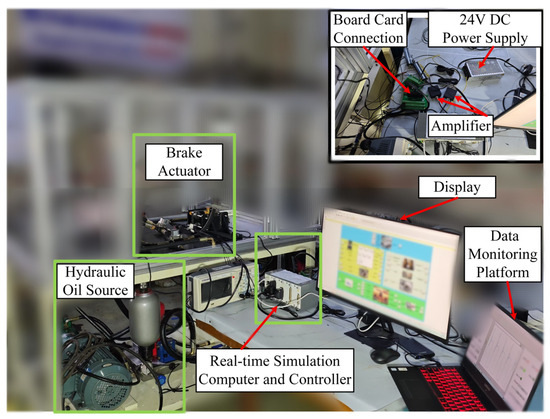
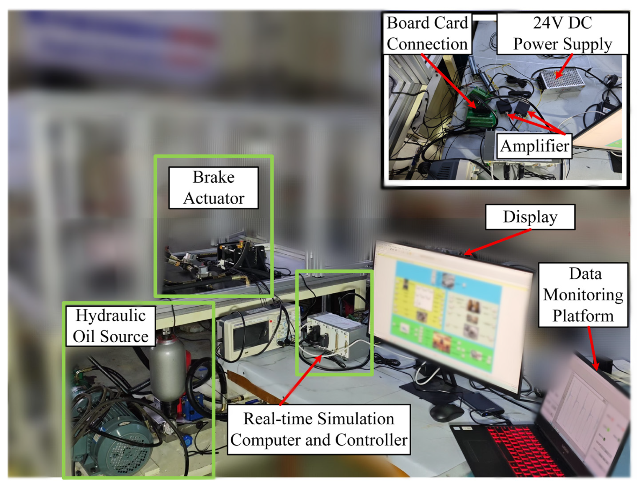
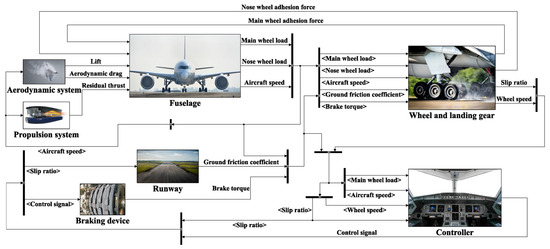
To validate the braking performance of the proposed anti-skid controller, comparative experiments are conducted on an anti-skid braking Hardware-in-the-Loop (HIL) test bench. The structure of the test bench is shown in Figure 6.

Figure 6. Hardware-in-the-Loop test bench.

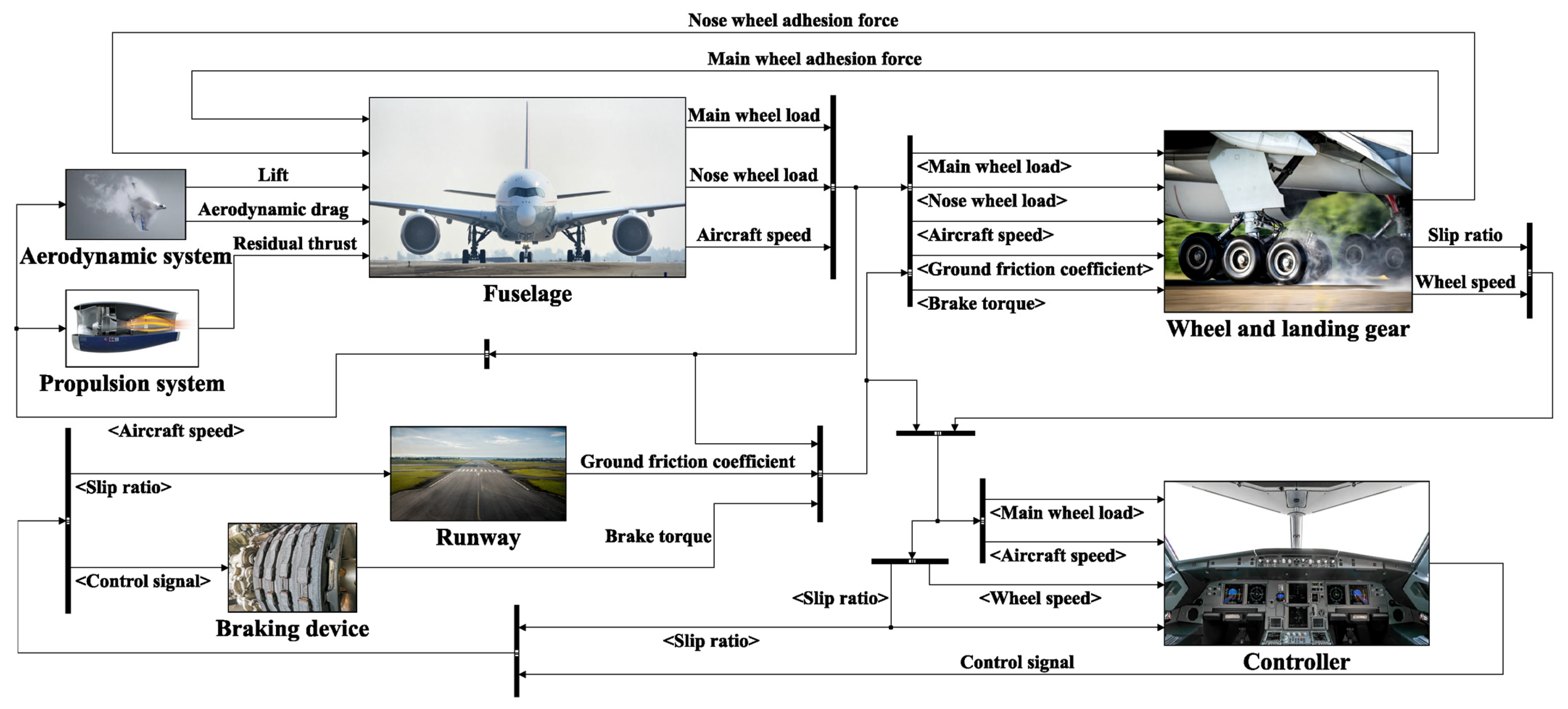
The HIL experiment, also known as semi-physical simulation, effectively enhances the confidence level of experiments by integrating physical hardware components with simulation software (MATLAB 2023a). Given the complex working characteristics of hydraulic braking systems, the test bench utilizes a real hydraulic braking system to execute braking actions in order to authentically validate the control performance of the proposed strategy in practical hydraulic braking scenarios. Furthermore, to facilitate the testing of multiple types of runway environments, the test bench uses an accurate runway model instead of an inertial platform. The HIL test bench primarily consists of a hydraulic braking system, a real-time simulator and controller, a display, and a data monitoring platform, among other components. The real-time simulator contains an aircraft dynamics simulation model used to simulate the entire aircraft braking process; the model structure is shown in Figure 7.

Figure 7. Simulink simulation model on the real-time simulator.

The braking test procedure is as follows: First, the real-time simulator and controller are started with the set initial parameters, and the brake signal is sent to the hydraulic braking system. Next, the hydraulic braking system distributes braking pressure to the brake actuator according to this signal. At this point, various sensors collect the action signals of the brake actuator and transmit them to the real-time simulator and controller. Finally, the real-time simulation computer combines the received signals to further simulate the motion states of components such as the airframe and wheels, and outputs the control signal for the next working cycle in combination with the control strategy. The above steps are executed cyclically until the experiment ends, thereby realizing the closed-loop test of the braking system.

To fully validate the control performance of the proposed controller, three controllers are tested on the HIL bench: the traditional PBM controller, a PSO-based composite PID controller, and the proposed GQPSO-based composite PID controller. The PBM controller is retained as the engineering benchmark because it is a conventional and directly implementable anti-skid law for aircraft braking systems. The PSO-based controller provides an intelligent PID/optimization baseline with the same composite-control framework as the proposed method, so that the contribution of the Gaussian quantum optimization mechanism can be isolated. Because the composite controllers regulate the PID gains through offline lookup tables during the real-time braking process, the PSO and GQPSO parameter tables are generated under identical optimization settings before the HIL experiments; the iteration number is set to 10 and the swarm size is set to 18 for both algorithms. Beyond the stability screening under single-runway conditions, two abrupt-friction scenarios are considered: a dry–wet–dry runway and a dry–ice–dry runway. In both cases, the aircraft first rolls over 200 m of dry runway, then passes through a 200 m wet or icy section, and finally returns to a dry runway. These scenarios also provide a sensitivity test for rapid changes in the friction curve. The key parameters of the HIL test are shown in Table 1.

Table 1. Key parameters for the Hardware-in-the-Loop test.

Symbol	Explanation	Values
v (m/s)	Initial aircraft speed	72
vend (m/s)	Aircraft anti-skid disengagement speed	7
W (N)	Landing weight of aircraft	759,500
R (m)	Wheel radius	0.53
Jg (kg·m2)	Wheel moment of inertia	2.88
ε	Slip rate offset	−0.01
B	Stiffness factors of dry, wet, and icy runways	[10.0326, 8.2098, 12.2198]
C	Shape factors for dry, wet, and icy runways	[1.5344, 2.0192, 2.0875]
D	Peak factors for dry, wet, and icy runways	[0.8, 0.4, 0.18]
Kp	Proportional coefficient of the PBM controller	53.7851
Ki	Integral coefficient of the PBM controller	0.2872
Kd	Differential coefficients of the PBM controller	0.1255
Kpz	Proportional coefficient range of the controller	[20, 62]
Kiz	Integral coefficient range of the controller	[0.025, 56]
Kdz	Differential coefficient range of the controller	[0.05, 0.78]
$\beta \left(\mathrm{t}\right)$	Contraction–expansion coefficient	[0.22, 0.55]
$w_1$	Penalty coefficient for slip rate error	1
$w_2$	Penalty coefficient for brake torque change rate	0.002
Tc (ms)	Control period	10

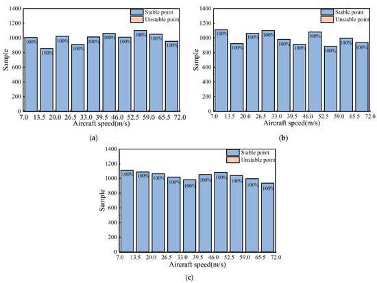
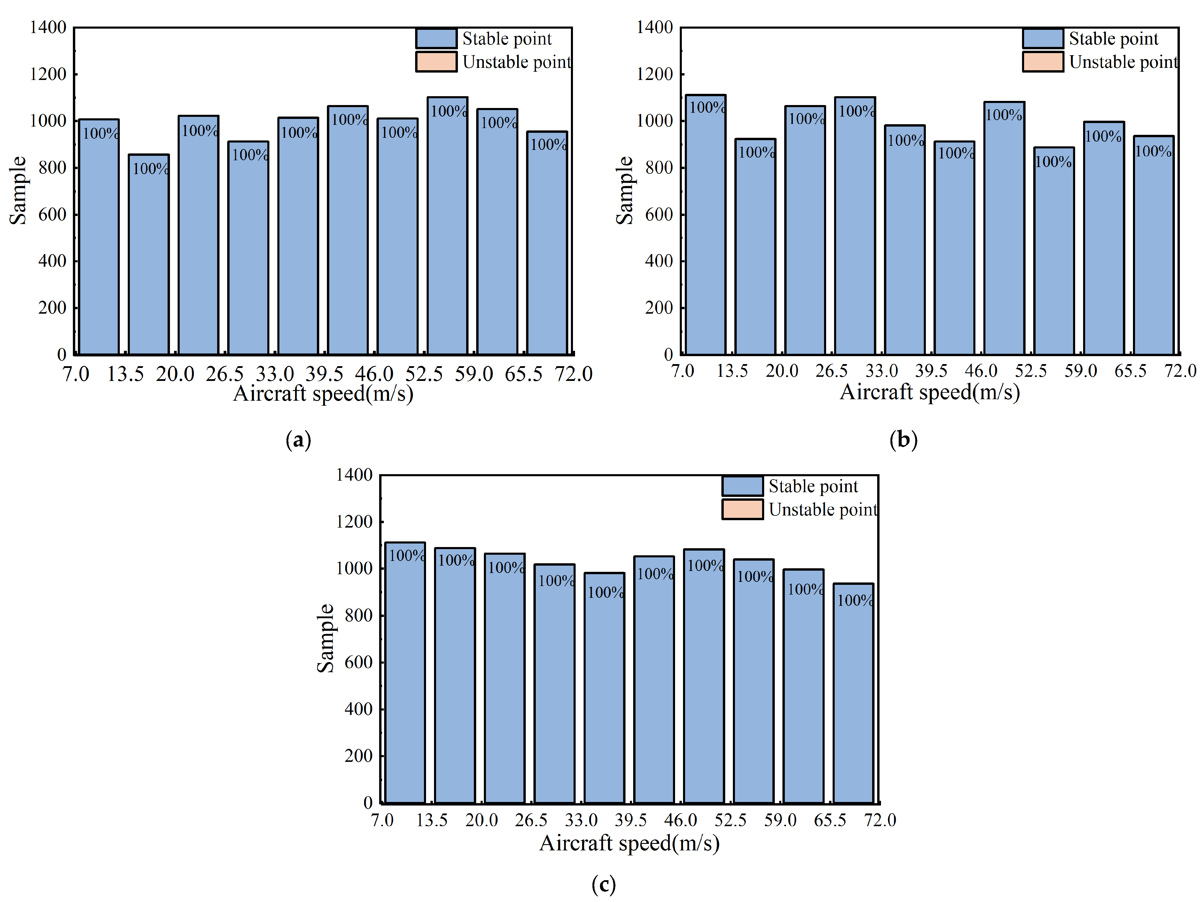
Before the experimental test, combined with the content in Section 3.3, the stability of the controller parameters under dry, wet, and icy runway conditions is first analyzed. The sample size of MCS is set to $N = 10,000$. The analysis results are shown in Figure 8. The results indicate that the control system remains stable within the verified sample space and exhibits a robust stability margin across different speed ranges and runway conditions. These trials evaluate the sensitivity of system stability against parameter deviations. The randomized nodes cover the operational envelope of aircraft speed and vertical load. The stable performance across these conditions indicates that the stability conclusions exhibit relatively low sensitivity to the violation of the constant-parameter assumptions. Furthermore, the sample distribution from the MCS is relatively uniform across the various speed ranges, indicating the good universality of the simulation results across speed ranges.

Figure 8. Stability analysis. (a) Analysis results on dry runway. (b) Analysis results on wet runway. (c) Analysis results on icy runway.

The offline generation of the multi-dimensional parameter lookup table is a critical step in the proposed control strategy. To construct a high-quality parameter matrix more rapidly across various conditions, an efficient optimization algorithm is required. Therefore, the performance of the adopted GQPSO is compared with that of the standard PSO algorithm.

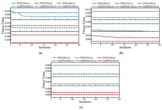
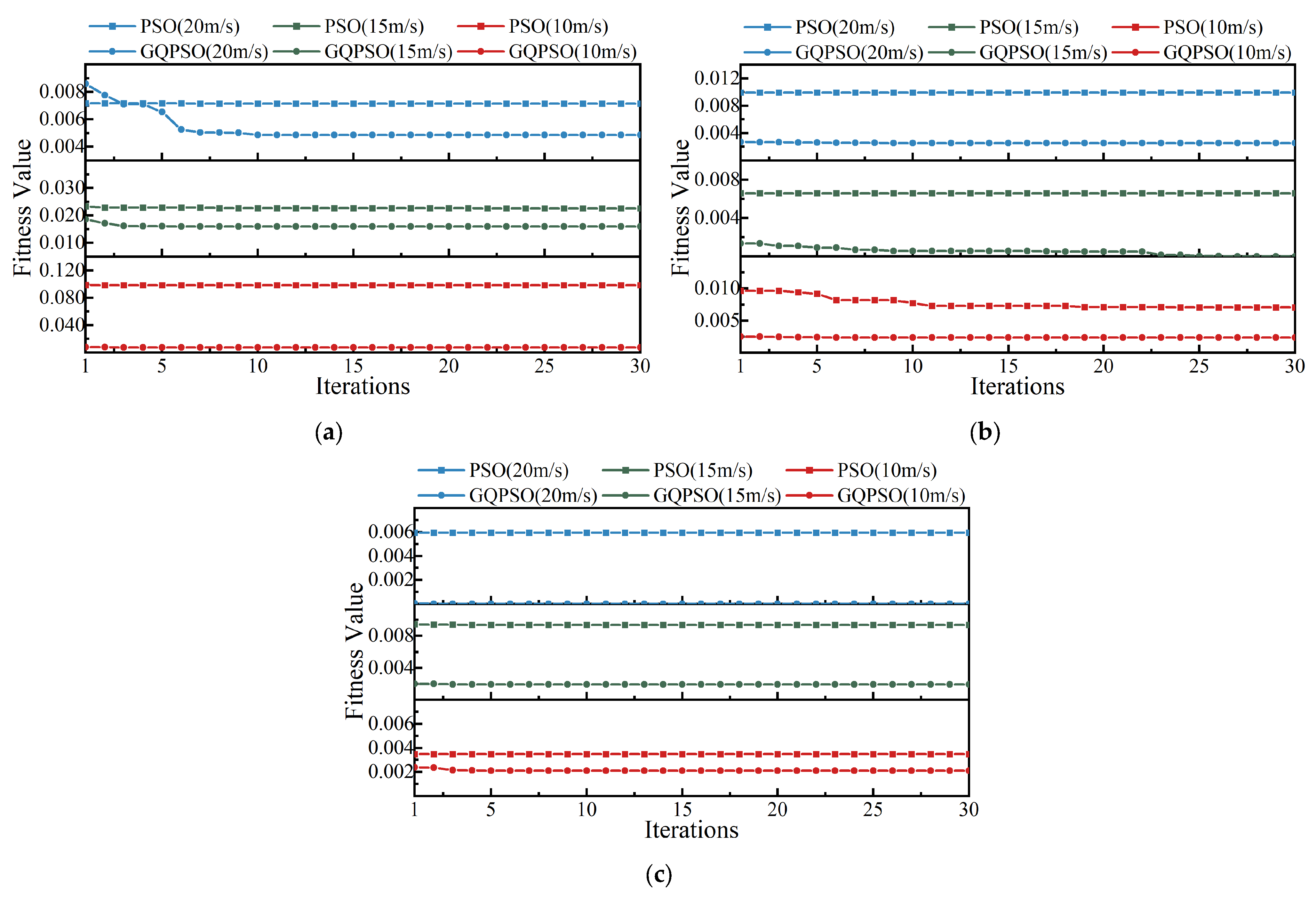
The optimization processes of both algorithms are recorded at aircraft speeds of 10 m/s, 15 m/s, and 20 m/s under dry, wet, and icy runway conditions, with the number of iterations set to 30. The corresponding convergence curves are presented in Figure 9. As illustrated in the figure, GQPSO consistently converges to lower fitness values and at a faster rate than PSO across all tested scenarios. The PSO frequently exhibits premature convergence, becoming trapped in sub-optimal local minima. This indicates that GQPSO is capable of searching for better PID parameters within a limited number of iterations.

Figure 9. Convergence performance comparison between PSO and GQPSO at different aircraft speeds. (a) Results on dry runway. (b) Results on wet runway. (c) Results on icy runway.

If configured with a larger swarm size and an extended number of iterations, the PSO algorithm might also obtain comparable optimal parameters. However, the PSO is susceptible to premature convergence and is sensitive to the initial particle distribution. Utilizing it for the generation of a multi-dimensional offline lookup table would consume excessive computational resources and is prone to yielding local optimal solutions. In contrast, by incorporating quantum mechanics principles and Gaussian mutation operators, GQPSO ensures faster convergence rates and superior global search stability. Based on the multi-dimensional parameter lookup table generated by GQPSO, the HIL experiments are subsequently conducted.

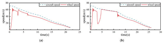
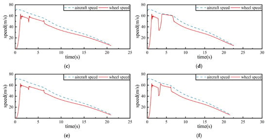
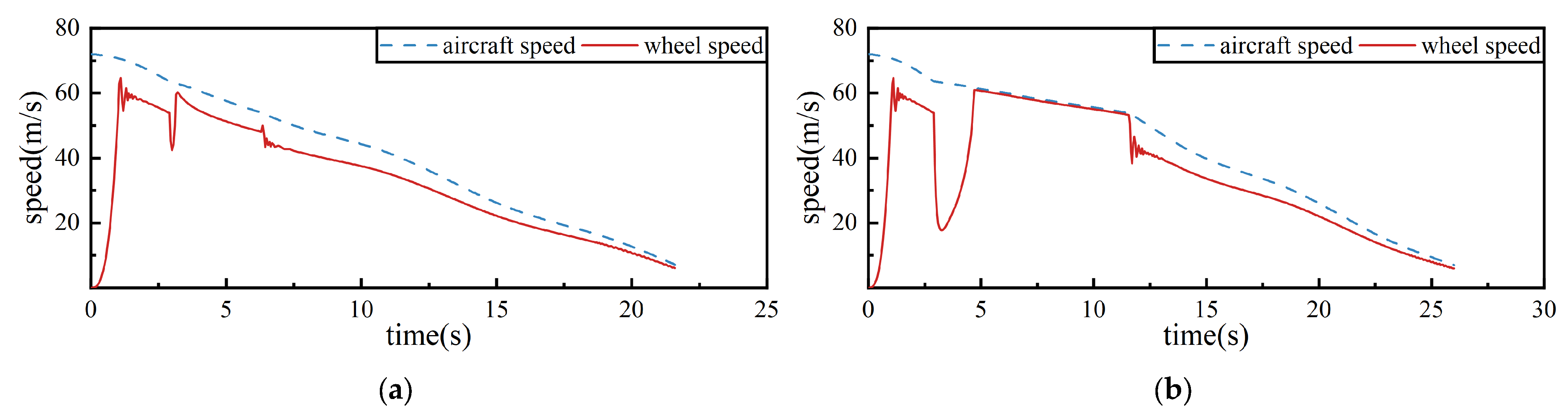
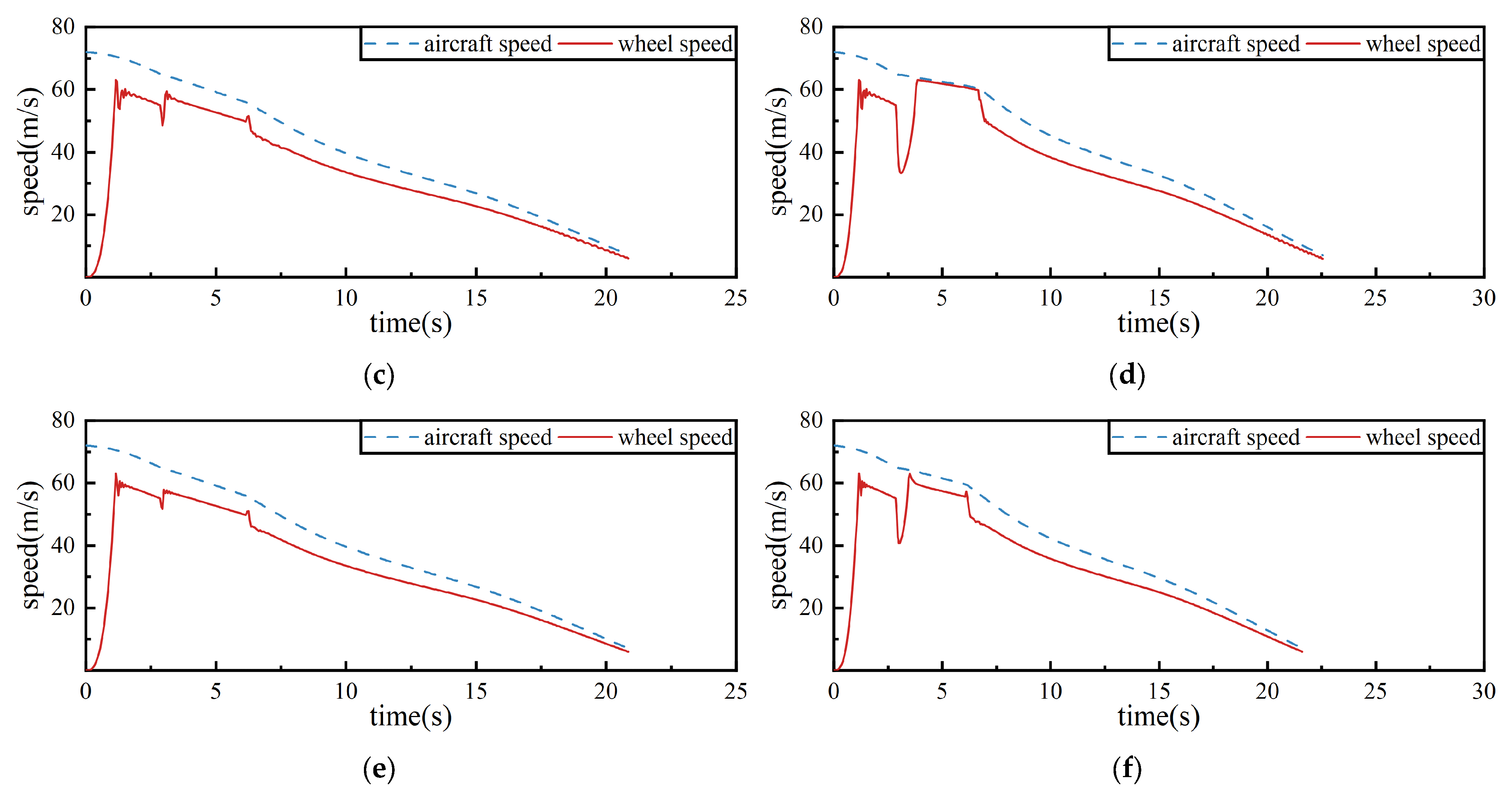
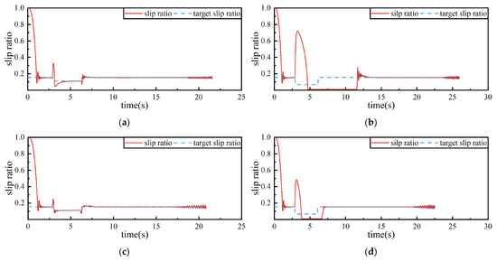
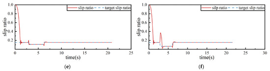
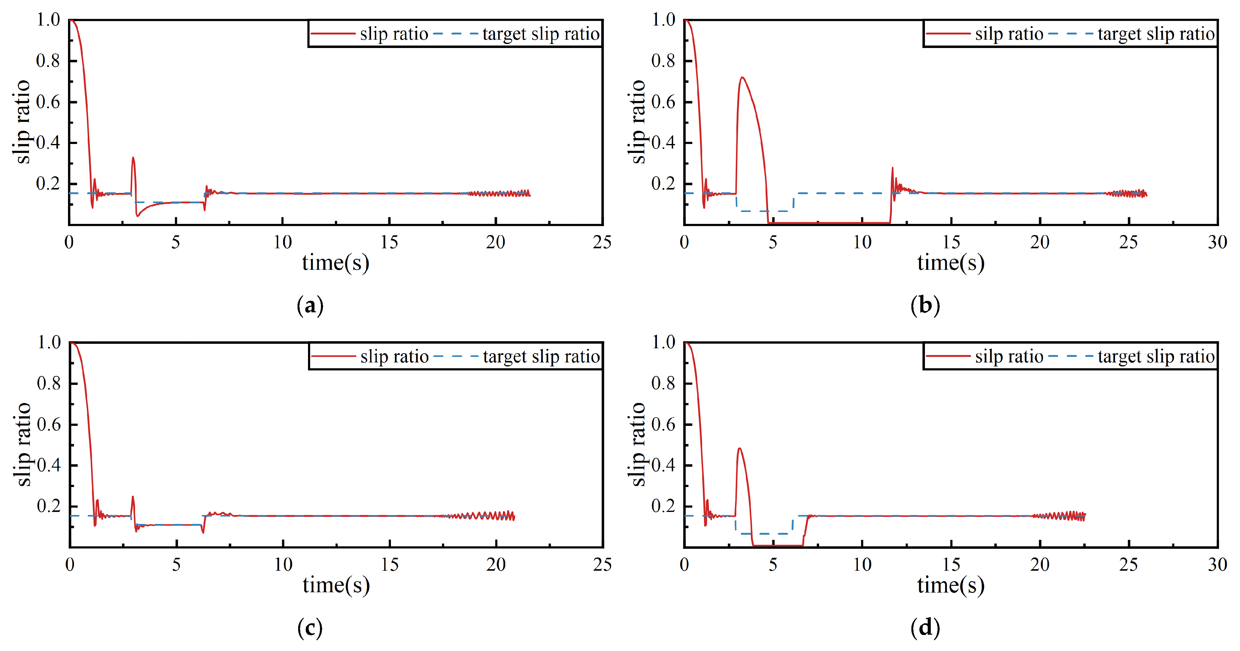
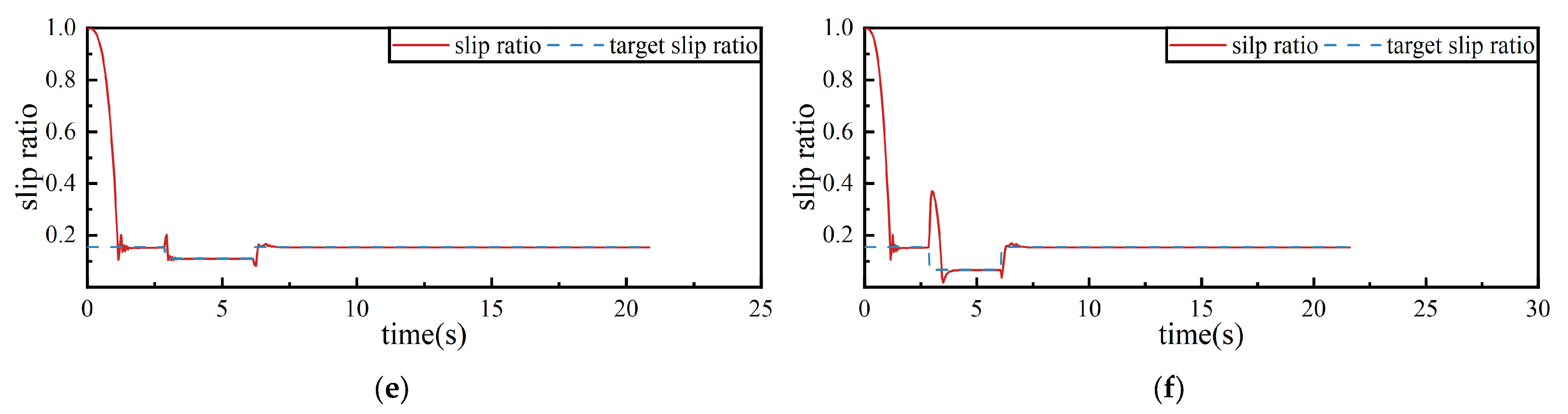
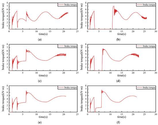
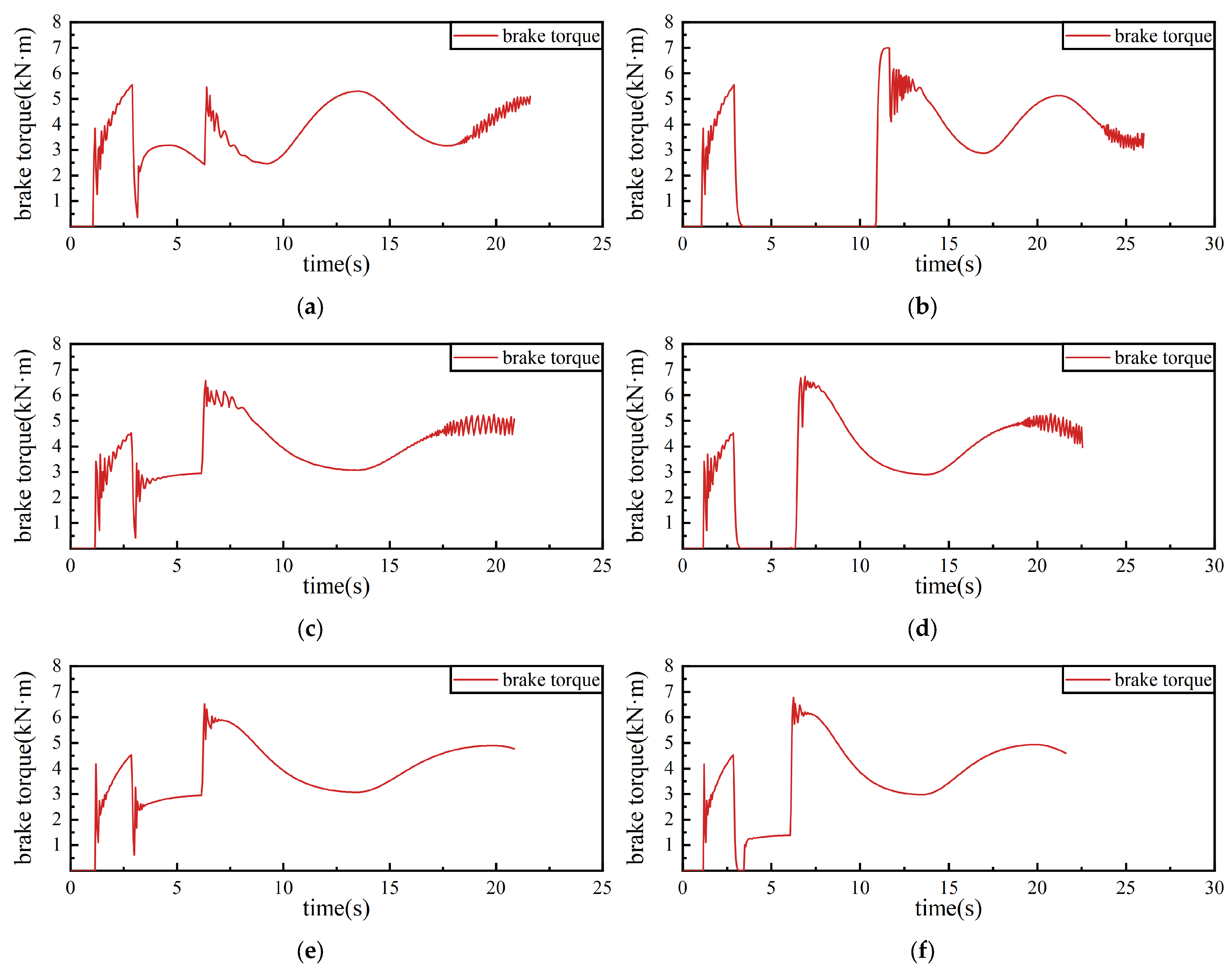
The results of the anti-skid braking HIL experiments are shown in Figure 10, Figure 11 and Figure 12, which illustrate the variations in aircraft speed, slip ratio, and braking torque, respectively, under the control of different controllers (traditional PBM controller, PSO-based composite controller and GQPSO-based composite controller) on dry–wet mixed runways and dry–ice mixed runways.

Figure 10. Variations in airframe speed and wheel speed under different controllers. (a) Experimental results of the PBM controller on a dry–wet mixed runway. (b) Experimental results of the PBM controller on a dry–ice mixed runway. (c) Experimental results of the PSO-based composite controller on a dry–wet mixed runway. (d) Experimental results of the PSO-based composite controller on a dry–ice mixed runway. (e) Experimental results of the GQPSO-based composite controller on a dry–wet mixed runway. (f) Experimental results of the GQPSO-based composite controller on a dry–ice mixed runway.

Figure 11. Aircraft slip ratio variations under different controllers. (a) Experimental results of the PBM controller on a dry–wet mixed runway. (b) Experimental results of the PBM controller on a dry–ice mixed runway. (c) Experimental results of the PSO-based composite controller on a dry–wet mixed runway. (d) Experimental results of the PSO-based composite controller on a dry–ice mixed runway. (e) Experimental results of the GQPSO-based composite controller on a dry–wet mixed runway. (f) Experimental results of the GQPSO-based composite controller on a dry–ice mixed runway.

Figure 12. Brake torque variations under different controllers. (a) Experimental results of the PBM controller on a dry–wet mixed runway. (b) Experimental results of the PBM controller on a dry–ice mixed runway. (c) Experimental results of the PSO-based composite controller on a dry–wet mixed runway. (d) Experimental results of the PSO-based composite controller on a dry–ice mixed runway. (e) Experimental results of the GQPSO-based composite controller on a dry–wet mixed runway. (f) Experimental results of the GQPSO-based composite controller on a dry–ice mixed runway.

From Figure 10a,c,e, it can be observed that no distinct discrepancy in braking time is exhibited by the three controllers under the dry–wet mixed runway. Specifically, braking times of 21.640 s, 20.883 s, and 20.866 s are recorded under the PBM controller, the PSO-based controller, and the GQPSO-based controller, respectively. Nevertheless, compared with PBM and PSO-PID, the shortest braking time is still achieved by the proposed GQPSO-based controller. From Figure 11a,c,e, it can be observed that no large separation in slip-ratio tracking is shown by the three controllers under the dry–wet mixed runway. However, compared with PBM and PSO-PID, the target slip ratio is tracked more closely by the GQPSO-based controller. Specifically, when the runway transition occurs, the target slip ratio is re-attained after 0.231 s by the PBM controller, after 0.162 s by the PSO-PID controller, and after 0.114 s by the GQPSO-based controller. Furthermore, a smaller overshoot as well as weaker fluctuation are exhibited by this proposed controller. Specifically, under the PBM controller, a maximum slip-ratio error of 0.220 is generated. Similarly, a maximum slip-ratio error of 0.140 is exhibited under the PSO-PID controller. By comparison, a maximum error of 0.106 is yielded by the GQPSO-based controller. The difference is rendered much clearer under the dry–ice mixed runway. Under the operation of PBM and PSO-PID, low-speed skidding is exhibited by the wheels at low aircraft velocities. Conversely, the target slip ratio is stably maintained in the neighborhood by the GQPSO-based controller even in the low-speed phase.

From Figure 10b,d,f, a distinct discrepancy in braking time is clearly exhibited by the three controllers under the dry–ice mixed runway. Specifically, braking times of 26.002 s, 22.560 s, and 21.639 s are recorded under the PBM controller, the PSO-PID controller, and the GQPSO-based controller, respectively. Compared with the results obtained under the dry–wet mixed runway, a significant prolongation in braking time is experienced by the PBM controller. Meanwhile, an increase in braking time is also exhibited by both the PSO-PID and GQPSO-PID controllers. Nevertheless, a more pronounced extension is manifested by the PSO-PID controller than by the proposed GQPSO-based method.

From Figure 11b,d,f, it can be observed that compared with the case under the dry–wet mixed runway, deviations of varying degrees in tracking the target slip ratio are exhibited by all three controllers when the runway transition occurs. However, compared with the PBM controller and the PSO-PID controller, a faster recovery to the neighborhood of the target slip ratio as well as a smaller overshoot are achieved by the GQPSO-based controller. Specifically, during the abrupt runway transition, the neighborhood of the target slip ratio is never re-attained by the PBM controller, whereby tracking instability is induced; furthermore, after the runway returns to the dry condition, 5.492 s is still required by this controller to re-enter the target slip ratio, and another 1.458 s is needed for stabilization to be achieved on it. A similar tracking instability is exhibited under the PSO-PID controller as the target neighborhood is never returned to during the transition phase; nevertheless, after returning to the dry runway, the target slip ratio is re-entered within only 0.880 s, and stabilization is achieved after an additional 0.071 s. By contrast, stabilization in the neighborhood of the new target slip ratio is achieved by the GQPSO-based controller within only 0.851 s after the runway transition; furthermore, the target slip ratio is tracked within only 0.172 s when returning to the dry runway, and stabilization on it is attained after another 0.696 s. In addition, a smaller maximum overshoot is exhibited by this proposed controller throughout the entire process. Specifically, a maximum overshoot of 0.654 is generated under the PBM controller. Similarly, an overshoot of 0.419 is exhibited under the PSO-PID controller. By comparison, a maximum overshoot of only 0.306 is yielded by the GQPSO-based controller. Thus, it is demonstrated that a smaller overshoot can still be maintained by the proposed controller even under harsh environments, whereby the occurrence of deep skidding is suppressed. Additionally, consistent with the case under the dry–wet mixed runway, low-speed skidding is exhibited by both the PBM and PSO-PID controllers in the low aircraft velocity phase. Detailed data can be found in Table 2.

Table 2. The effects of different controllers on mixed runways.

Runway	Controller	Rise Time (s)	Setting Time (s)	Overshoot
Dry–wet	PBM	0.231 s (dry–wet), 0.117 s (wet–dry)	1.142 s (dry–wet), 0.680 s (wet–dry)	0.220
Dry–wet	PSO-PID	0.162 s (dry–wet), 0.159 s (wet–dry)	0.458 s (dry–wet), 1.318 s (wet–dry)	0.140
Dry–wet	GQPSO-PID	0.114 s (dry–wet), 0.127 s (wet–dry)	0.242 s (dry–wet), 0.491 s (wet–dry)	0.106
Dry–ice	PBM	1.756 s (dry–ice), 5.492 s (wet–ice)	None (dry–ice), 6.950 s (ice–dry)	0.654
Dry–ice	PSO-PID	0.901 s (dry–ice), 0.880 s (wet–ice)	None (dry–ice), 0.951 s (ice–dry)	0.419
Dry–ice	GQPSO-PID	0.547 s (dry–ice), 0.172 s (wet–ice)	0.851 s (dry–ice), 0.696 s (ice–dry)	0.306

A consistent difference among the three controllers is shown by the brake torque responses in Figure 12. In Figure 12a,b, frequent torque release and re-application are produced by PBM after the friction changes. In Figure 12c,d, part of this fluctuation is reduced by PSO-PID. However, relatively frequent torque variation is still exhibited by this controller, especially on the dry–ice mixed runway. In Figure 12e,f, a smoother brake-torque command with smaller variation is generated by the GQPSO-based controller. High-frequency actuation of the braking device can be reduced by this smoother torque regulation.

In the dry–wet mixed runway, braking efficiencies of 94.38%, 95.16%, and 95.46% are achieved by PBM, PSO-PID, and GQPSO, respectively. Corresponding stopping distances of 872.07 m, 846.74 m, and 845.84 m are recorded. Thus, an improvement of 1.08 percentage points over PBM and 0.30 percentage points over PSO-PID in braking efficiency is achieved by GQPSO. Meanwhile, reductions of 3.01% and 0.11% in the stopping distance are yielded, respectively. A much larger advantage is manifested in the dry–ice mixed runway. Specifically, braking efficiencies of 63.22%, 79.45%, and 94.23% are obtained under PBM, PSO-PID, and GQPSO, respectively. The corresponding stopping distances are measured as 1128.24 m, 957.94 m, and 899.28 m. Therefore, increments of 31.00 percentage points over PBM and 14.77 percentage points over PSO-PID in braking efficiency are provided by GQPSO. Additionally, the stopping distance is shortened by 20.29% and 6.12%, respectively.

Under the dry–wet mixed runway, the target slip ratio can be tracked quickly and stably by both PBM and PSO-PID. Thus, only minor performance discrepancies are manifested between these two baseline controllers and GQPSO-PID. However, due to the issue of low-speed skidding and small tracking deviations, lower braking efficiencies and longer stopping distances are still exhibited by PBM and PSO-PID relative to GQPSO-PID. Conversely, a different behavior is shown under the dry–ice mixed runway. When the abrupt runway transition occurs, the target slip ratio cannot be tracked in a timely manner by either PBM or PSO-PID. Concurrently, large overshoots are produced by both controllers. Consequently, a dramatic decrease in braking efficiency is caused, and the stopping distance is substantially elongated. In contrast, the target slip ratio can still be tracked quickly and stably by GQPSO-PID despite the abrupt runway variation. Therefore, a high braking efficiency and a shorter stopping distance are successfully maintained by the proposed controller.

The principle behind low-speed skidding can be explained by the definition of slip ratio. A larger change in the slip ratio is produced by the same wheel-speed disturbance when a low aircraft speed is encountered. Under the traditional PBM controller, sufficient adaptation to this speed-dependent sensitivity cannot be achieved by the fixed control parameters. As a result, a high susceptibility to low-speed skidding and repeated brake release is manifested. Under the PSO-PID controller, the adjustment of the PID gains can be performed through an offline lookup table. However, a slower convergence rate is exhibited by the standard PSO algorithm. Additionally, a high tendency towards entrapment in a local optimum is shown by this standard algorithm. Under limited iteration and particle swarm size, suboptimal PID parameters are easily generated due to the weaker optimization capability. Consequently, a larger overshoot and poorer tracking performance are induced when a sharp change in runway friction is encountered. By contrast, a stronger global search capability and a faster convergence speed are demonstrated by the GQPSO algorithm. Thus, more suitable PID parameters can be provided for the transition process. Ultimately, smaller overshoot, faster recovery speed, and smoother torque regulation are reflected.

To further evaluate the repeatability and mass sensitivity of the proposed GQPSO-based controller, repeated experiments are conducted under different aircraft masses on a dry runway. These repeated experiment results are presented in Table 3.

Table 3. Data from repeated experiments.

Number	Aircraft Quality	Brake Time	Brake Distance	Maximum Slip Rate Error
1	Cargo 20%	19.486 s	749.62 m	0.113
2	Cargo 20%	19.334 s	747.25 m	0.106
3	Cargo 20%	19.389 s	750.08 m	0.105
4	Cargo 40%	19.452 s	754.72 m	0.080
5	Cargo 40%	19.506 s	758.21 m	0.095
6	Cargo 40%	19.574 s	757.39 m	0.116
7	Cargo 60%	19.648 s	765.53 m	0.091
8	Cargo 60%	19.772 s	769.03 m	0.111
9	Cargo 60%	19.759 s	770.96 m	0.104
10	Cargo 80%	19.796 s	774.03 m	0.107
11	Cargo 80%	19.789 s	771.50 m	0.102
12	Cargo 80%	19.822 s	775.02 m	0.083
13	Cargo 100%	19.878 s	777.45 m	0.067
14	Cargo 100%	19.947 s	781.87 m	0.098
15	Cargo 100%	19.880 s	778.04 m	0.078

The repeatability experiments are carried out for cargo conditions of 20%, 40%, 60%, 80%, and 100%. For each aircraft mass level, three repeated trials are performed. Therefore, this analysis is reported in the form of descriptive statistics and a linear trend assessment rather than a formal hypothesis test.

An increase from 19.403 s to 19.902 s in the mean braking time is observed as the cargo condition is increased from 20% to 100%. Concurrently, an increase from 748.98 m to 779.12 m in the mean braking distance is recorded. Within-group coefficients of variation below 0.40% for the braking time and below 0.36% for the braking distance are obtained. Through these indices, a small run-to-run dispersion at each mass level is indicated. A least-squares fit is performed using all 15 trials. A regression slope of 0.385 m in the braking distance per 1% cargo increase is yielded by this fit. Concurrently, a coefficient of determination of 0.953, a residual standard error of 2.60 m, and a maximum absolute residual of 5.58 m are generated. When the fit is applied to the five group means, the coefficient of determination is increased to 0.976. Meanwhile, a maximum residual of 3.13 m is manifested. Compared with the 30.14 m increase in the mean braking distance from 20% to 100% cargo, these residuals are found to be small. Consequently, a systematic mass effect is suggested, while limited uncertainty in the repeated tests is implied. The maximum slip-ratio error is generally confined between 0.067 and 0.116. A weak mass dependence is exhibited by the regression analysis of the slip-ratio error, where a coefficient of determination of 0.296 and an RMSE of 0.0117 are yielded. In summary, it is demonstrated by the results that repeatable braking performance can be maintained by the proposed controller under different aircraft mass levels.

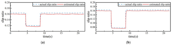
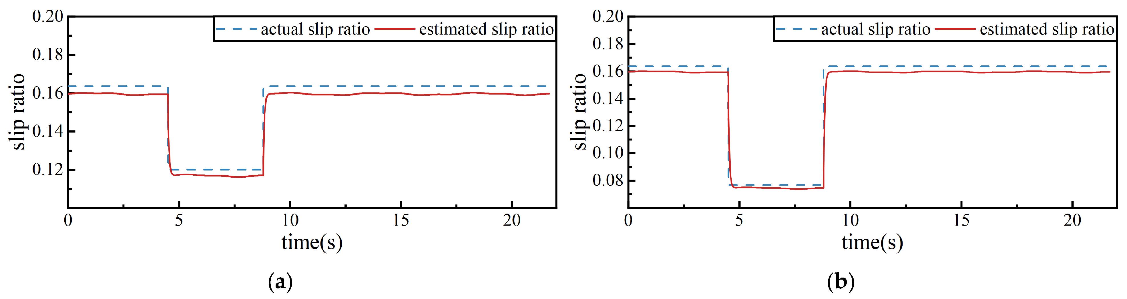
For a more intuitive demonstration of the effectiveness of the runway identification module, a direct comparison between the actual and estimated optimal slip ratios is conducted. These variations are shown in Figure 13.

Figure 13. Runway identification results. (a) Runway identification results of dry–wet mixed runway. (b) Runway identification results of dry–ice mixed runway.

As shown in Figure 13a, the dry–wet–dry transition trend is well tracked by the identified value. A mean absolute error of 0.00398 and a root-mean-square error (RMSE) of 0.00433 are obtained. As shown in Figure 13b, a larger instantaneous step is exhibited under the dry–ice mixed runway. Nevertheless, the dry–ice–dry transition trend is still well tracked by the identified value. In this scenario, a mean absolute error of 0.00401 and an RMSE of 0.00533 are generated. Although a lag behind the actual value is manifested by the identified value at the two sudden transitions, a short delay is produced. Specifically, a delay time within 0.05–0.09 s is recorded under the dry–wet mixed runway. Meanwhile, a delay of approximately 0.09–0.13 s is exhibited under the dry–ice mixed runway. Therefore, the actual optimal slip ratio can be rapidly tracked by the identification module. Concurrently, a small residual error is maintained. Consequently, the requirements for use as the target slip ratio reference of the composite anti-skid controller are satisfied.

In summary, more stable slip-ratio tracking is achieved by the proposed GQPSO-based composite controller than by the PBM and PSO-PID controllers. Higher braking efficiency, shorter braking distance, and faster recovery after runway changes are obtained under the tested mixed runway conditions. The runway identification module also provides acceptable optimal-slip-ratio estimation, with small errors and short delays after sudden runway changes. The repeated tests under different mass levels further indicate that stable and repeatable braking performance can be maintained.

5. Conclusions

To address the issues of runway condition uncertainty and low-speed skidding, a composite anti-skid braking strategy based on GQPSO is developed. The strategy is evaluated through HIL experiments and compared with PBM and PSO-PID under mixed runway conditions. The main conclusions and future research directions are summarized as follows:

(1)

A BPNN-based runway identification method based on main-wheel dynamics and friction characteristics is developed. This module provided the target slip-ratio reference for the controller and demonstrated small estimation errors in the mixed-runway tests. This result supports its application as an identification-assisted reference module in the proposed strategy.

(2)

A GQPSO-based PID scheduling strategy is proposed. The PID gains are optimized offline and implemented through lookup tables, thereby reducing online computational demand. Under abrupt runway changes, the GQPSO-PID controller achieved smoother torque regulation as well as faster and more stable slip-ratio tracking compared with PBM and PSO-PID.

(3)

Phase-plane analysis and MCS are utilized to screen the feasible PID parameter space before HIL testing. The results indicate that the selected controller parameters remain within the verified stable region under the tested runway and speed ranges.

(4)

The HIL tests demonstrate that the proposed controller can maintain stable slip-ratio tracking under both dry–wet and dry–ice mixed runways. This advantage is particularly evident on the dry–ice mixed runway, where deep skidding is effectively suppressed and braking efficiency is improved. Large-scale repetitive testing also indicates good repeatability of braking performance within the tested range.

(5)

The present study still includes simplified measurement assumptions. The runway identification module utilizes vertical load and braking-torque-related information from the main wheels. In practical deployment, the vertical load may be obtained from landing-gear load sensors or strain gauges, whereas the braking torque usually needs to be estimated from brake pressure rather than measured directly. Therefore, future work will focus on the accurate estimation of load and braking torque, brake thermal effects, and further experimental validation of the runway identification method.

References

- Li, R.; Qiao, W.; Liu, X.; Jin, H.; Gao, X.; Li, D.; Wu, S.; Shang, Y.; Jiao, Z. A novel dual-redundancy more-electric braking system and regulation strategy based on on/off valves. IEEE/ASME Trans. Mechatron. 2024, 29, 4594–4605. [Google Scholar] [CrossRef] [Scilit]
- Jiao, Z.; Zhang, H.; Shang, Y.; Liu, X.; Wu, S. A power-by-wire aircraft brake system based on high-speed on-off valves. Aerosp. Sci. Technol. 2020, 106, 106177. [Google Scholar] [CrossRef] [Scilit]
- Jiao, Z.; Liu, X.; Shang, Y.; Huang, C. An integrated self-energized brake system for aircrafts based on a switching valve control. Aerosp. Sci. Technol. 2017, 60, 20–30. [Google Scholar] [CrossRef] [Scilit]
- Jiao, Z.; Bai, N.; Liu, X.; Li, Y.; Wang, Z.; Sun, D.; Qi, P.; Shang, Y. Aircraft anti-skid braking control technology: A review. Acta Aeronaut. Astronaut. Sin. 2022, 43, 450–474. [Google Scholar] [CrossRef]
- Yan, Y.; Gan, X.; Wu, Y.; Yang, L. Aircraft landing safety quality analysis based on modified FRAM method. J. Beijing Univ. Aeronaut. Astronaut. 2022, 49, 1964–1973. [Google Scholar] [CrossRef]
- Huang, J.; Zhang, X.; Meng, C.; Tian, Q.; Xu, D. Effect of thrust reverser on the deceleration performance of civil aircraft. J. Aerosp. Power 2023, 38, 728–734. [Google Scholar] [CrossRef]
- Chung, H.S. Computational investigations of adverse effects of deploying spoilers on airfoil aerodynamic characteristics. J. Korean Soc. Aeronaut. Space Sci. 2020, 48, 335–342. [Google Scholar] [CrossRef] [Scilit]
- Wang, X.L.; Wang, F.X.; Li, Y.L. Aerodynamic characteristics of high-lift devices with downward deflection of spoiler. J. Aircr. 2011, 48, 730–735. [Google Scholar] [CrossRef] [Scilit]
- Korba, P.; Huňady, R.; Hovanec, M.; Racek, B.; Pavelka, P. Fatigue life analysis of an aircraft brake component to prevent damage and ensure operational safety. Eng. Fail. Anal. 2021, 129, 105653. [Google Scholar] [CrossRef] [Scilit]
- Cui, J.; Zhang, N.; Cui, X.; Wang, J.; Yu, M.; Liu, D.; Jiang, L. Fault diagnosis method of aircraft anti-skid brake system based on GWO-PNN. In Proceedings of the 2021 33rd Chinese Control and Decision Conference, Kunming, China, 22–24 May 2021. [Google Scholar] [CrossRef] [Scilit]
- Li, J.; Zhu, K.; Fang, W. Key technologies of high speed aircraft braking system. Aerosp. Technol. 2024, 457, 17–22. [Google Scholar] [CrossRef]
- Xu, F.; Liang, X.; Chen, M.; Liu, W. Robust self-learning PID control of an aircraft anti-skid braking system. Mathematics 2022, 10, 1290. [Google Scholar] [CrossRef] [Scilit]
- Zhao, G.; Yin, Q.; Zhang, S.; Wei, X.; Nie, H. All-electric braking control method for UAVs based on hierarchical PID. Acta Aeronaut. Astronaut. Sin. 2026, 47, 32760. [Google Scholar] [CrossRef]
- Wang, Z.; Liu, X.; Qi, P. Brake-induced landing gear walk vibration analysis and suppression method research. J. Aircr. 2024, 61, 1218–1229. [Google Scholar] [CrossRef] [Scilit]
- Zhao, P.; Liang, N.; Yuan, Z.; Lu, J.; Zeng, Z. The design of adaptive anti-skid control based on the slip rate constraints. In Proceedings of the 2018 3rd International Conference on Mechanical, Control and Computer Engineering, Hangzhou, China, 22–23 October 2018. [Google Scholar] [CrossRef] [Scilit]
- Lei, X.; Gao, G.; Li, B.; Liu, S.; Qu, Q. Research and development on advanced technology of aircraft brake system. J. Air Force Eng. Univ. 2022, 23, 8–16. [Google Scholar] [CrossRef]
- Wang, Z.; Bai, N.; Liu, X.; Qi, P. Observer-based adaptive robust control of aircraft antiskid brakes with disturbance compensation. Control Eng. Pract. 2024, 152, 106079. [Google Scholar] [CrossRef] [Scilit]
- Chen, J.; Wang, J.; Wang, W. Robust adaptive control for nonlinear aircraft system with uncertainties. Appl. Sci. 2020, 10, 4270. [Google Scholar] [CrossRef] [Scilit]
- Prach, A.; Gürsoy, G.; Yavrucuk, L. Nonlinear controller for a fixed-wing aircraft landing. In Proceedings of the 2019 American Control Conference, Philadelphia, PA, USA, 10–12 July 2019. [Google Scholar] [CrossRef] [Scilit]
- Chen, M.; Xu, F.; Liang, X.; Liu, W. MSD-based NMPC aircraft anti-skid brake control method considering runway variation. IEEE Access 2021, 9, 51793–51804. [Google Scholar] [CrossRef] [Scilit]
- Du, C.; Li, F.; Yang, C.; Shi, Y.; Liao, L.; Gui, W. Multiphase-based optimal slip ratio tracking control of aircraft antiskid braking system via second-order sliding-mode approach. IEEE/ASME Trans. Mechatron. 2021, 27, 823–833. [Google Scholar] [CrossRef] [Scilit]
- Fu, L.; Tian, G.; Wang, P.; Liang, B.; Huangfu, Y. Adaptive sliding mode control strategy for the aircraft antiskid braking system based on slip ratio. J. Northwest. Polytech. Univ. 2015, 33, 770–774. [Google Scholar]
- Zhang, X.; Lin, H. Backstepping fuzzy sliding mode control for the antiskid braking system of unmanned aerial vehicles. Electronics 2020, 9, 1731. [Google Scholar] [CrossRef] [Scilit]
- Chen, X.; Wang, H.; Yan, X.; Yang, J. Control of aircraft anti-skid braking system considering nonlinear factors. Control Theory Appl. 2022, 39, 950–958. [Google Scholar] [CrossRef]
- Papa, G.; Schiano, P.; Tanelli, M.; Panzani, G.; Savaresi, S.M. A wheel slip control scheme for aeronautical braking applications based on neural network estimation. Eur. J. Control 2022, 68, 100691. [Google Scholar] [CrossRef] [Scilit]
- Papa, G.; Tanelli, M.; Panzani, G.; Savaresi, S.M. A comparison of model-based and black-box methods for speed estimation in aircraft. IFAC-PapersOnLine 2020, 53, 14775–14780. [Google Scholar] [CrossRef] [Scilit]
- Chen, Y.; Tan, R.; Zheng, Y.; Zhou, Z. Sliding-mode control with multipower approaching law for dc-link voltage of z-source photovoltaic inverters. IEEE Access 2019, 7, 133812–133821. [Google Scholar] [CrossRef] [Scilit]
- Xiong, J.; Gu, H. Research on a sliding mode variable structure control FOC of PMSM for electric vehicles. In Proceedings of the 2018 IEEE 9th International Conference on Software Engineering and Service Science, Beijing, China, 23–25 November 2018. [Google Scholar] [CrossRef] [Scilit]
- Chen, F.; Ding, S.; Dong, Y. Research on control strategy of explosion-proof door based on BP neural network optimized fuzzy PID control. Mod. Manuf. Eng. 2022, 507, 111. [Google Scholar] [CrossRef]
- Lin, X.; Li, K.; Wang, L. A driving-style-oriented adaptive control strategy based PSO-fuzzy expert algorithm for a plug-in hybrid electric vehicle. Expert Syst. Appl. 2022, 201, 117236. [Google Scholar] [CrossRef] [Scilit]
- Ławryńczuk, M. Nonlinear model predictive control for processes with complex dynamics: A parameterisation approach using Laguerre functions. Int. J. Appl. Math. Comput. Sci. 2020, 30, 35–46. [Google Scholar] [CrossRef] [Scilit]
- Liu, Y.; Wu, H.; Wang, L.; Ge, Q.; Zhu, X. A review of unmanned systems research based on neurodynamic optimization. Control Decis. 2025, 40, 2049–2069. [Google Scholar] [CrossRef]
- Vega, F.; Yu, W. Fuzzy modeling using LSTM cells for nonlinear systems. In Proceedings of the 2020 IEEE International Conference on Fuzzy Systems, Glasgow, UK, 19–24 July 2020. [Google Scholar] [CrossRef] [Scilit]
- Wang, M.; Yang, X.; Qian, Y.; Lei, Y.; Cai, J.; Huan, Z.; Lin, X.; Dong, H. Adaptive neural network structure optimization algorithm based on dynamic nodes. Curr. Issues Mol. Biol. 2022, 44, 817–832. [Google Scholar] [CrossRef] [Scilit] [PubMed]
- Sun, G.; Li, S.; Yu, Q.; Zhang, J. Enhancing position control in pneumatic systems using ANFIS and high-speed on-off valves with compound PWM. Int. J. Hydromechatron. 2024, 7, 347–367. [Google Scholar] [CrossRef] [Scilit]
- Cunegatto, E.H.T.; Zinani, F.S.F.; Rigo, S.J. Multi-objective optimisation of micromixer design using genetic algorithms and multi-criteria decision-making algorithms. Int. J. Hydromechatron. 2024, 7, 224–249. [Google Scholar] [CrossRef] [Scilit]
- Kanungo, A.; Kumar, P.; Gupta, V.; Salim; Saxena, N.K. A design an optimized fuzzy adaptive proportional-integral-derivative controller for anti-lock braking systems. Eng. Appl. Artif. Intell. 2024, 133, 108556. [Google Scholar] [CrossRef] [Scilit]
- He, Q.; Zheng, H.; Ma, X.; Wang, L.; Kong, H.; Zhu, Z. Artificial intelligence application in a renewable energy-driven desalination system: A critical review. Energy AI 2022, 7, 100123. [Google Scholar] [CrossRef] [Scilit]
- Xu, F.; Chen, M.; Liang, X.; Liu, W. PSO optimized active disturbance rejection control for aircraft anti-skid braking system. Algorithms 2022, 15, 158. [Google Scholar] [CrossRef] [Scilit]
- Jennan, N.; Mellouli, E.M. Optimal fixed-time sliding mode control for anti-lock braking systems based fuzzy logic and neural network. Results Eng. 2025, 25, 103921. [Google Scholar] [CrossRef] [Scilit]
- Li, L.; Zhang, X.; Fu, Y.; Ma, X. Parameter optimization of aircraft brake control law based on improved particle swarm optimization algorithm. Fire Control Command Control 2024, 49, 41–48. [Google Scholar] [CrossRef]
- Merrouche, W.; Lekouaghet, B.; Bouguenna, E. Gaussian quantum-behaved PSO strategy for lithium battery model optimization. In Proceedings of the International Symposium on Quantum Sciences: Applications and Challenges, Algiers, Algeria, 24–25 September 2023; pp. 107–119. [Google Scholar] [CrossRef] [Scilit]
- Ishak Boushaki, S.; Bendjeghaba, O.; Kamel, N.; Salhi, D.E. Enhanced gaussian quantum particle swarm optimization for the clustering of biomedical data. In Proceedings of the International Symposium on Quantum Sciences: Applications and Challenges, Algiers, Algeria, 24–25 September 2023; pp. 38–49. [Google Scholar] [CrossRef] [Scilit]
- Concepcion, R.; Dadios, E.; Alejandrino, J.; Mendigoria, C.H.; Aquino, H.; Alajas, O.J. Diseased surface assessment of maize cercospora leaf spot using hybrid gaussian quantum-behaved particle swarm and recurrent neural network. In Proceedings of the 2021 IEEE International IOT, Electronics and Mechatronics Conference, Toronto, ON, Canada, 21–24 April 2021. [Google Scholar] [CrossRef] [Scilit]
- Mendoza Lopetegui, J.J.; Finotto, G.; Tanelli, M. Gain-scheduled design of active braking control systems for optimized ground handing in aircraft. In Proceedings of the 2024 European Control Conference (ECC), Stockholm, Sweden, 25–28 June 2024. [Google Scholar] [CrossRef] [Scilit]
- Mendoza Lopetegui, J.J.; Tanelli, M. Robust electro-hydraulic control for aircraft anti-skid systems with full validation from test bench to flight. Control Eng. Pract. 2026, 169, 106814. [Google Scholar] [CrossRef] [Scilit]
- Crocetti, F.; Fravolini, M.; Costante, G.; Valigi, P. Data-driven and uncertainty-aware robust airstrip surface estimation. Neural Comput. Appl. 2023, 35, 19565–19580. [Google Scholar] [CrossRef] [Scilit]
- Zhao, J.; Wu, X.; Song, Z.; Sun, H. State estimation of tractor semi-trailer based on improved particle filter. J. Hunan Univ. (Nat. Sci.) 2025, 52, 14–23. [Google Scholar] [CrossRef]
- Pacejka, H.B. Tire and Vehicle Dynamics; Butterworth-Heinemann: Amsterdam, The Netherlands, 2012. [Google Scholar]
- Liu, Y.; Li, D. AdaXod: A new adaptive and momental bound algorithm for training deep neural networks. J. Supercomput. 2023, 79, 17691–17715. [Google Scholar] [CrossRef] [Scilit]
- Schmidt, K. Aircraft Wheels, Brakes, and Brake Controls: Key Principles for Landing Gear Design; SAE International: Warrendale, PA, USA, 2022. [Google Scholar]
- Dos Santos Coelho, L. Gaussian quantum-behaved particle swarm optimization approaches for constrained engineering design problems. Expert Syst. Appl. 2010, 37, 1676–1683. [Google Scholar] [CrossRef] [Scilit]
Disclaimer/Publisher’s Note: The statements, opinions and data contained in all publications are solely those of the individual author(s) and contributor(s) and not of MDPI and/or the editor(s). MDPI and/or the editor(s) disclaim responsibility for any injury to people or property resulting from any ideas, methods, instructions or products referred to in the content. |
© 2026 by the authors. Licensee MDPI, Basel, Switzerland. This article is an open access article distributed under the terms and conditions of the Creative Commons Attribution (CC BY) license.