


Abstract
The bonding between cabin sections and exterior shells represents a critical manufacturing operation in shell assembly, directly determining the reliability and structural performance of the assembled structure. However, traditional manual scraping suffers from low efficiency, poor consistency, and heavy reliance on manual operation, while conventional teach-and-repeat robotic automation fails to adapt to significant manufacturing tolerances and complex surface curvatures common in large-scale shell components. To address these challenges, this paper proposes a vision-guided robotic scraping method that generates adaptive trajectories on irregular cabin sections. The method achieves full pipeline integration and is particularly suited for production lines where various models share similar macro-geometries but possess subtle geometric variations. A system integrating a laser profile sensor is developed to perceive surface geometry and local normal vectors. By establishing a unified coordinate transformation chain and a scan–mesh–spline workflow, the sensed geometric information is directly mapped to the robot end-effector pose. A trajectory generation algorithm based on point cloud meshing and B-spline interpolation is employed to construct continuous, smooth scraping paths that accommodate geometric deviations without relying on complex fixtures. Unlike RGB-D correction-based methods that require pre-programmed initial trajectories, or CAD-driven offline programming that cannot adapt to manufacturing deviations, the proposed approach directly generates conformal scraping paths from measured geometry. Experimental results on a typical cabin section demonstrate that the generated trajectories accurately follow the surface normals, achieving a low standard deviation of 36 μm in adhesive layer thickness, indicating excellent thickness consistency and uniformity. Furthermore, the automated process reduced the total operation time to approximately 40 min, improving production efficiency by more than two times compared to manual operations, thereby validating the robustness and suitability of the method for high-precision batch manufacturing.
1. Introduction
With the advancement of industrial manufacturing technology, surface treatment processes for irregular components have become a critical factor affecting workpiece performance and reliability [1]. In the field of spacecraft structural assembly, the bonding quality between irregular parts and protective layers directly determines the service life and safety of the workpiece. Therefore, automated scraping technology has gradually developed into an emerging direction in intelligent manufacturing [2]. Automated scraping systems for irregular cabin sections feature controllable costs, high production efficiency, and flexible adaptation of process modules [3]. Combined with digital modeling and real-time quality monitoring technology, they significantly improve the consistency of the scraping process and workpiece yield [4]. In aerospace assembly, the acceptable tolerance of adhesive layer thickness is typically on the order of tens of micrometers, imposing stringent requirements on both geometric conformity and process stability.
The bonding between spacecraft cabin sections and exterior shells is a critical process in shell assembly. The consistency of adhesive layer thickness, boundary neatness, and overall uniformity are directly related to service reliability and structural performance [5]. In engineering practice, two-component adhesives are commonly used, which are characterized by strong thixotropy, high viscosity, sensitivity to environmental temperature and humidity and surface cleanliness, and limited operating time [6]. Currently, such bonding processes are primarily performed manually. However, manual methods generally suffer from low efficiency, poor stability, large variations in adhesive layer thickness, and severe boundary overflow and contamination. These issues make it difficult to meet current requirements for quality consistency and batch production cycle time, highlighting an urgent need for automation [7].
For automatic scraping of complex curved surfaces, industrial robots have been explored in various related manufacturing scenarios. Compared with general manufacturing scenarios, spacecraft cabin assembly imposes significantly stricter requirements due to complex free-form geometries, cabin deformation, and stringent tolerance constraints on adhesive thickness. Nevertheless, these existing studies still provide valuable insights and methodological references for the problem addressed in this work. Some of these scenarios rely on regular geometry or fixed fixtures, where process paths are pre-taught and then repeatedly executed, supplemented by quantitative adhesive supply to obtain good [8]. Maiolino et al. developed a robotic sealant dispensing system for aircraft manufacturing in which RGB-D sensor data were utilized to adaptively correct pre-programmed offline trajectories, thereby improving the flexibility of robotic operations under geometric variability [9]. Leali et al. investigated an offline programming approach for robotic deburring of aerospace components, comparing CAD-based and digitizer-based strategies to improve flexibility and efficiency in processing complex and variable geometries [10]. However, trajectory correction methods typically involve a manual teaching process to define the initial trajectory, which reduces operational efficiency. Guo et al. proposed a versatile method based on weighted locally optimal projection (WLOP) to directly generate machining paths from point cloud data [11], but did not consider process-aware constraints such as adhesive thickness compensation. To handle non-uniform geometries, Pušnik and Hace proposed a region-based framework that subdivides the surface according to local curvature features to optimize robotic motion dynamics and path efficiency [12]. To address the inefficiency of grinding complex aluminum alloy surfaces with weld defects, Zhao et al. proposed a defect positioning method combining 2D images with 3D point clouds and a space spiral trajectory planning strategy to improve grinding efficiency and surface quality [13]. Li et al. proposed a floating grinding actuator utilizing a composite force–position fuzzy control strategy to overcome the reliance on precise geometric pre-measurement in traditional grinding [14]. To address the precision and efficiency issues in traditional free-form surface polishing, Song et al. proposed an improved trajectory planning method based on curvature-based dynamic partitioning and a hybrid optimization framework combining Genetic Algorithm and Local Search to enhance trajectory smoothness and machining quality [15]. These VGR methods from manufacturing practices offer valuable insights for the present work.
However, existing research still has some deficiencies: (1) Existing vision-based methods typically rely on predefined trajectories generated via offline programming or manual teaching, and mainly perform trajectory correction based on sensor feedback, lacking the capability of directly generating task-specific trajectories from measured geometry. This is especially significant for production lines where different models share similar macro-geometries but possess subtle variations, as our method eliminates the need for labor-intensive recalibration; (2) Manufacturing and clamping errors, as well as in situ deformation of cabin sections and exterior shells, often reach levels causing teach-and-repeat offline paths to easily mismatch under field deviations [4]; (3) Finished product quality thresholds are higher, with requirements for adhesive layer thickness consistency, edge quality, and cleanliness significantly stricter than those in general manufacturing scenarios [7]. The manual acceptance standard now for thickness standard deviation is 100 μm, an automated workflow is essential to avoid thickness fluctuations and inconsistencies caused by varying levels of manual operation skills.
To address these challenges, this paper proposes a vision-guided robotic scraping method that uses a laser profiler to perceive cabin surface geometry. By establishing a coordinate transformation chain, the measured geometric information is directly mapped to the robot end-effector pose and trajectory correction, thereby achieving adaptive control of adhesive layer thickness under conditions of manufacturing and clamping deviations.
The main contributions of this paper are:
- Proposing a vision–motion collaborative framework for irregular cabin sections, clarifying the transformation relationships between sensor coordinate systems, robot base, flange, and tool coordinate systems, and cabin coordinate systems, and providing the mapping path from measured surface geometry to robot end-effector tool pose and trajectory.
- Presenting a scraping pose generation and thickness compensation approach based on local normals and tooling geometry, which ensures robust adhesive layer thickness control and path conformity under geometric deviations.
- Achieving a full pipeline integration from vision perception to automated scraping execution. Compared to RGB-D correction-based methods, the proposed approach eliminates the need for pre-programming of initial robotic trajectories, thereby significantly improving operational efficiency. Meanwhile, unlike traditional CAD-driven offline programming, it is capable of dynamically compensating for actual manufacturing tolerances and deformations of the cabin sections.
The remainder of this paper is structured as follows. The proposed vision-guided robotic scraping framework and adaptive trajectory generation method are first described, including system configuration and coordinate transformation modeling. Subsequently, experimental results are presented to validate the effectiveness of the approach in terms of trajectory accuracy, thickness consistency, and operational efficiency. Finally, concluding remarks and future research directions are provided.
2. Materials and Methods
2.1. Cabin Surface Scraping System
2.1.1. System Components and Functions
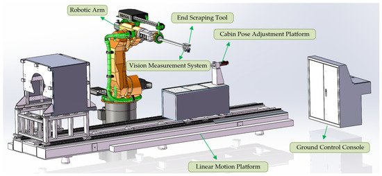
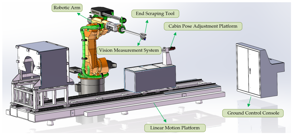
The cabin shell surface scraping system mainly consists of a linear motion platform, cabin pose adjustment platform, robotic arm with end scraping tool, vision measurement system, and ground control console. As shown in Figure 1.
Figure 1.
System composition.
The linear motion platform is responsible for the overall long-stroke linear movement of the workstation and carrying the upper-level devices. The cabin pose adjustment platform mounted on it is used to fix and support the cabin model, providing multi-degree-of-freedom position and attitude fine-tuning capabilities. The robotic arm, equipped with an end scraping tool, is responsible for adhesive mixing, supply, and trajectory-based scraping. The vision measurement system uses a laser profiler to online acquire target geometry and attitude. The ground control console coordinates and schedules all subsystems, generates motion and process control commands.
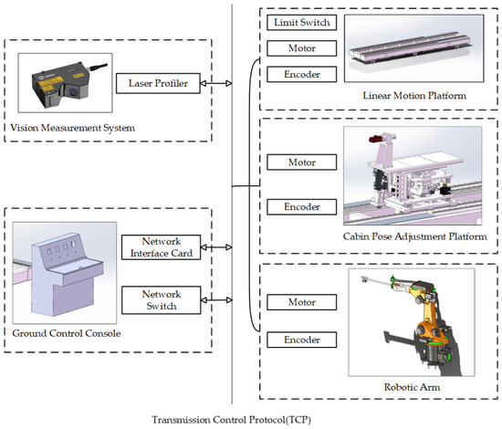
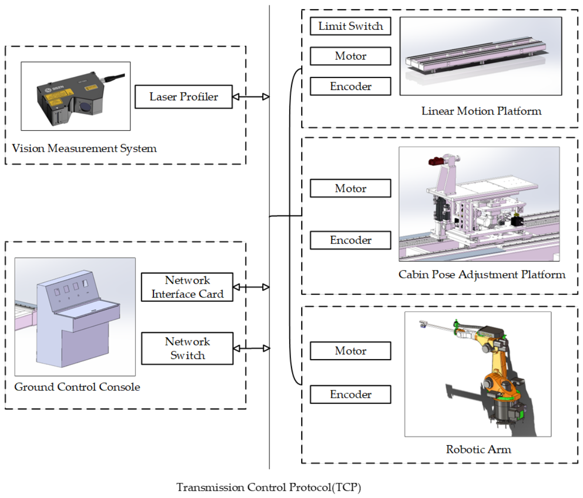
As shown in Figure 2, the system employs a centralized master–slave control hierarchy. The ground control console acts as the master node, while the vision measurement system, robotic arm, and motion platform function as slave nodes. The communication relies on a TCP network protocol via the network switch. During the perception phase, spatial synchronization between the laser profiler and the robot end-effector is achieved through timestamp-matching. The profiler continuously captures 3D features while the robot controller records joint encoder data at high frequency. During the scraping execution phase, the ground control console transmits the generated trajectory to the robot’s lower-level controller. Meanwhile, the master console maintains a lower-frequency supervisory loop to monitor limit switches and global state parameters, ensuring stable and collision-free operations.
Figure 2.
System electrical connection.
2.1.2. Coordinate System Definition
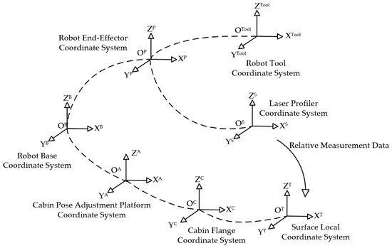
The cabin surface automatic scraping system defines the robot base, end-effector and tool coordinate systems, the cabin pose adjustment platform base coordinate system and cabin coordinate system [16], and defines the robot base coordinate system as the system reference coordinate system. The transformation relationships between coordinate systems are shown in Figure 3.
Figure 3.
Coordinate system transformation relationships, where , , , , , , and represent the coordinate systems of the robot base, end-effector, tool, laser profiler, adjustment platform, cabin flange, and surface local, respectively.
The system defines seven coordinate systems following the right-hand rule: robot base , cabin pose adjustment platform , cabin flange , robot end-effector , robot tool , laser profiler , and surface local . serves as the global reference with its X-axis aligned along the linear rail. and are fixed to the platform and cabin end flange respectively. and are centered at the robot’s sixth joint, while is rigidly attached to the tool frame for surface scanning. Finally, is established on each surface mesh cell, where the Z-axis aligns with the outward surface normal to guide the scraping orientation.
In practical implementation, the transformations were calibrated using a Hexagon Leica laser tracker.
2.2. System Coordinate Transformation Relations
2.2.1. Reference Coordinate System and Platform, Flange, and Surface Coordinate Systems
The robot base coordinate system serves as the system reference. The cabin pose adjustment platform coordinate system is basically parallel to , with only origin translation:
The cabin flange coordinate system coincides with when the platform is at zero position. When there is attitude adjustment on the platform, there is translation and rotation between them:
For each -th mesh cell on the cabin surface, a corresponding surface local coordinate system is defined. The homogeneous transformation from the surface local coordinate system to the cabin flange coordinate system is:
where is the position of the -th mesh center point from , and the third column of is consistent with the surface normal . Accordingly, the total transformation from the surface local coordinate to the base is:
2.2.2. Robot End-Effector and Tool Coordinate Systems
The pose of the robot end-effector coordinate system relative to is obtained from the DH chain [17] of joint angles :
where , , , are DH parameters.
The robot we use is KUKA KR70R2100. The transformation relationship between the end-effector system and the base system is represented by the robot D-H parameters, detailed in Table 1.
Table 1.
Robot D-H parameters.
The robot tool coordinate system has a length offset along relative to :
2.2.3. Laser Profiler Coordinate Unification
Let the laser profiler coordinate system be , rigidly mounted on tool , with relative pose:
Then the sensor-to-base and tool pose chains are respectively:
For point measured in , unified to base and tool [18]:
2.3. Scraping Trajectory Generation Algorithm
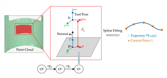
This section describes the method for generating spline scraping trajectories executable by the robotic arm from point clouds obtained by laser profiler scanning [19,20]. First, the point cloud acquired from laser profiling scans is spatially discretized into rectangular meshes based on the scraping tool’s effective width. Within each mesh, the geometric centroid is calculated to serve as the anchor point. To ensure the scraping tool conforms perfectly to the irregular cabin sections, the local tool pose is strictly defined by geometric constraints: the tool’s Z-axis is aligned with the surface normal derived from the local covariance matrix of the mesh points, while the scraping advance direction X-axis, is constructed to be orthogonal to the cabin’s central axis within the tangent plane. Subsequently, a thickness compensation is applied along the normal vector to determine the final target coordinate. Finally, these discrete target poses serve as control points for trajectory reconstruction, where B-spline fitting and quaternion spherical linear interpolation are employed to generate a smooth, continuous path that guarantees consistent coating thickness and stable tool orientation. As shown in Figure 4, the algorithm workflow converts raw point cloud data into executable robotic trajectories by integrating mesh-based feature extraction, coordinate transformation, thickness compensation, and spline-based path smoothing.
Figure 4.
Scraping trajectory generation algorithm workflow, where , , and represent the base, cabin flange, and surface local coordinate systems; , , , and denote the mesh centroid, surface normal, target control point, and thickness compensation, respectively.
2.3.1. Mesh Division and Control Point Extraction
To facilitate the discretization of continuous surfaces into several executable control units, rectangular mesh division is performed on the cabin surface according to the scraping tool width w and the laser profiler scan bandwidth . In regions where the cabin surface profile exhibits large curvature variations, the mesh size is adaptively reduced to densify the grid and ensure adequate control point resolution in geometrically complex areas. Let the -th mesh be:
where represents the point cloud set measured by the laser profiler and registered to the cabin coordinate system. The geometric range of each is approximately in regions of uniform curvature, with refined dimensions applied in high-curvature areas.
Define the center point centroid of the mesh as:
where is the point cloud coordinate. To determine the surface normal, local principal component analysis is adopted to calculate the local covariance matrix:
Perform eigenvalue decomposition on , and take the unit eigenvector corresponding to the minimum eigenvalue as the normal candidate . Unify the normal sign according to the outward-facing rule to obtain the unit normal [21]:
2.3.2. Local Tool Pose Determination
The desired orientation of the scraping tool in the mesh satisfies: the tool Z-axis is consistent with the surface normal, the tool X-axis, which points to the scraping advance direction, is perpendicular to the cabin central axis, and the tool y-axis is determined by the right-hand rule.
For the -th mesh, the desired scraping pose of the tool in satisfies: the tool axis aligns with the surface normal and maintains a gap along the normal:
The local pose obtained here can be expressed as a homogeneous transformation:
Using the coordinate transformation chain established in Section 2.2, the desired pose of the tool in the base coordinate system is:
where is the transformation from surface local coordinate to cabin flange coordinate , and , are the previously determined platform and base transformations.
2.3.3. Spline Fitting and Attitude Interpolation
The mesh control poses obtained in the previous subsection are ordered according to the trajectory traversal rule (row-by-row along the cabin axial direction). For each pose, the tool position extracted from is denoted as , and the corresponding orientation is . The position trajectory is generated by a three-dimensional B-spline [22,23] fitted to the ordered control points :
where denotes the ordered index set along the traversal path, and are the corresponding B-spline basis functions of order 3. For attitude interpolation, each is converted to a unit quaternion . Between adjacent control poses along the traversal order, the orientation is interpolated by spherical linear interpolation [24]:
Combining the interpolated position and the interpolated orientation yields the continuous tool trajectory .
3. Results
3.1. Experimental Verification
3.1.1. Evaluation of Point Cloud Measurement Data
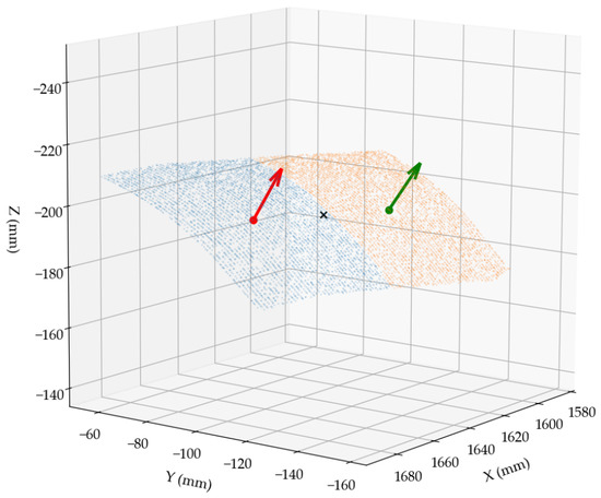
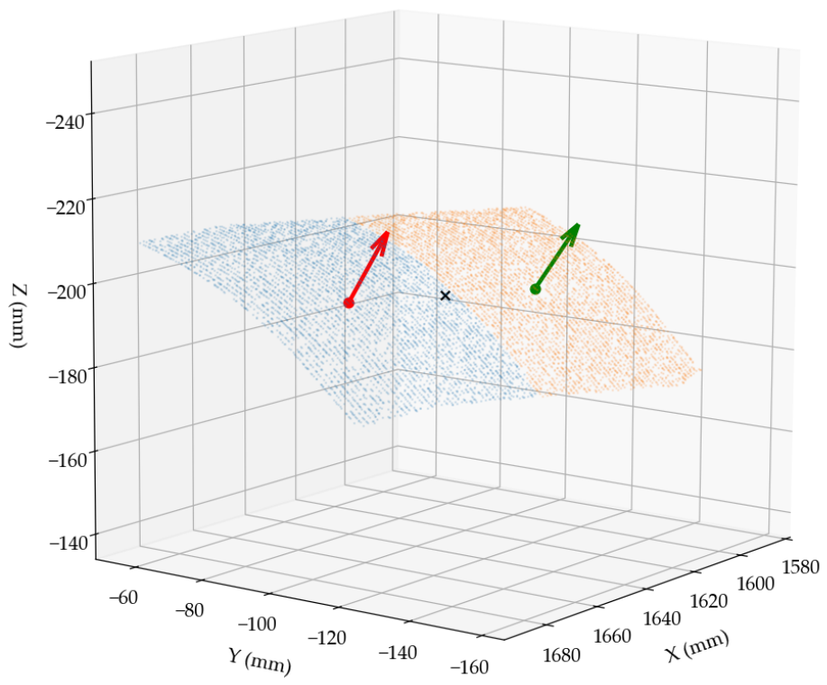
The laser profiler model selected for the vision measurement system is SSZN SR7140. An effective range is defined along the cabin axial direction, and all point cloud data outside this range are first removed. Subsequently, the statistical outlier removal (SOR) method is applied to filter out the remaining outliers [25]. The point cloud after outlier removal processing from a single scan is shown in Figure 5 and the local normal vectors is indicated by the red and green arrows.
Figure 5.
Point cloud example and normal vectors, where areas with different colors represent different point cloud meshes, and arrows indicate the surface normal vectors extracted by PCA for each corresponding mesh.
To evaluate high-frequency sensor noise, PCA is performed within a micro-neighborhood of radius since the variance of the point cloud along the normal direction, represented by the minimum eigenvalue, can directly quantify the local noise level near the sampled point. To evaluate the scanning uniformity, the point cloud region is divided into 25 cells. By calculating the standard deviation of the number of points in each cell and the sparsest point count, the non-uniformity is strictly evaluated. The evaluation results are summarized in Table 2.
Table 2.
Evaluation results of point cloud.
Data analysis shows that the system is mathematically sufficient to support stable covariance matrix calculations for surface normals. The normal vectors extracted from adjacent regions exhibit a smooth transition.
3.1.2. Experimental Environment and Parameter Settings
The experiment selected a typical metal cabin section as the working object. The cabin section mainly consists of a cylindrical section and an irregular transition curved surface, made of steel structure, and features a diameter of 450 mm and an axial length of 600 mm, and the theoretical adhensive thickness is set as 250 μm.
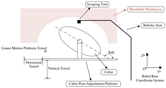
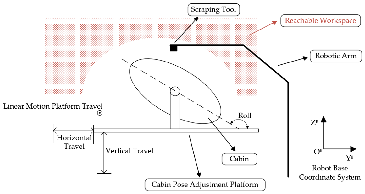
As shown in Figure 6, due to the limitation of the robot’s reachable workspace, the complete scraping process of a full cabin section is divided into two stages. In each stage, the cabin pose adjustment platform rotates the cabin such that the surface to be scraped is positioned upward and within the accessible workspace of the robotic arm. The two stages are geometrically symmetric; one of them is taken as a representative example.
Figure 6.
Schematic diagram of the experimental setup.
The motion range limitations of the experimental setup are summarized in Table 3.
Table 3.
Motion range of system components.
3.1.3. Trajectory Generation
Laser scanning and trajectory planning experiments were performed on the cabin section. After the laser profiler completed full-coverage scanning of the cabin surface, surface geometric features were extracted through point cloud preprocessing and meshing, and a total of 83 meshes were divided.
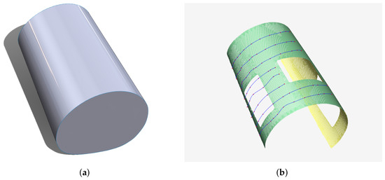
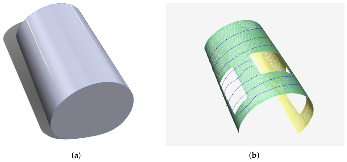
Figure 7a shows the theoretical cabin model, Figure 7b presents the three-dimensional point cloud model acquired from laser profiling scans, covering both the regular cylindrical section and irregular transition areas of the cabin, and also displays the scraping trajectories generated by the algorithm. The red control point sequence is positioned at the geometric center of each mesh cell, and the continuous blue trajectory from B-spline interpolation follows the point cloud surface smoothly. The generated trajectory orientations correctly track surface normal variations across regions of varying curvature.
Figure 7.
(a) Theoretical cabin model. (b) Generated scraping trajectories on the point cloud.
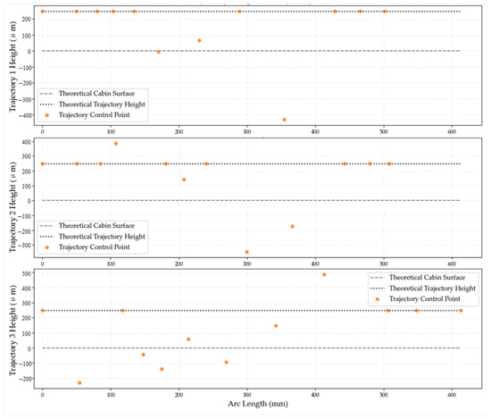
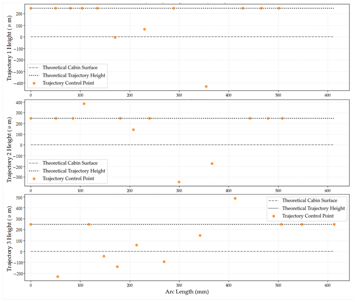
Figure 8 presents the height deviation profile along three representative trajectory of eight total trajectories, comparing the theoretical trajectory height against the actual calculated trajectory height. The actual trajectory height is computed by the proposed algorithm based on the laser-scanned point cloud of the real cabin section. Observable deviations ranging from approximately −400 μm to +400 μm reflect the geometric discrepancies between the as-manufactured cabin section and its theoretical model. These variations demonstrate the capability of the adaptive trajectory generation algorithm to compensate for manufacturing tolerances and achieve conformal scraping paths that accommodate real-world geometric deviations.
Figure 8.
Comparison between theoretical and actual trajectory heights.
3.1.4. Adhesive Layer Thickness Consistency Analysis
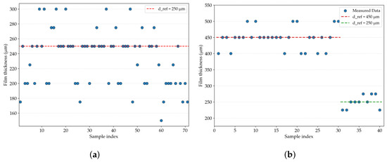
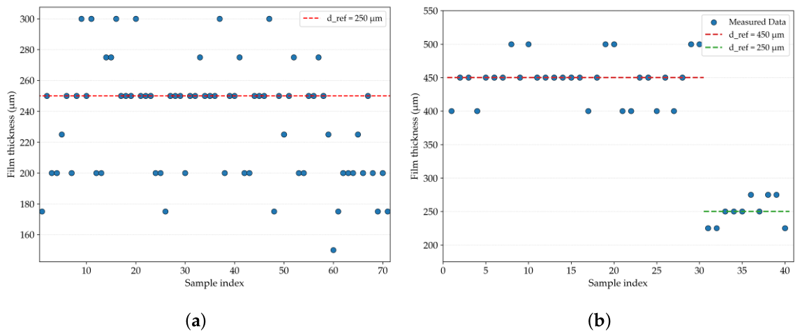
After completing automatic scraping, oil film gauges were used for multi-point uniform sampling measurement of the adhesive layer, and a total of 71 feature points were selected on the cabin section. The adhesive used in this experiment has a viscosity of 20,000 mPa·s. The measurement results distribution of adhesive layer thickness are shown in Figure 9a.
Figure 9.
(a) Thickness distribution measurement results of cabin 1. (b) Thickness distribution measurement results of cabin 2.
To verify the robustness of the proposed method under different cabin curvatures and adhesive properties, an additional experiment was conducted on a second cabin section with a diameter of 500 mm and an axial length of 475 mm, using a higher-viscosity adhesive (80,000 mPa·s). The experimental results are shown in Figure 9b. This cabin section consists of two regions: one region requires an adhesive layer thickness of 250 μm, while the remaining area requires a thickness of 450 μm.
The statistical results as shown in Table 4 indicate that the proposed automated scraping method is effective across different cabin geometries and target thicknesses. The robot’s repeatability is ±0.05 mm, the depth repeatability of the laser profiler is 0.5 μm and the width repeatability is 8 μm, and the repeated positioning accuracy of the cabin pose adjustment platform is 0.025 mm. Since the cabin pose adjustment platform does not move during the scanning and adhesive application process in a single task, it is considered that the main error originates from the robot. Meanwhile, due to the self-leveling of the adhesive after application, a negative mean deviation occurs, and the fluctuation of the adhesive layer thickness becomes smaller than the robot positioning error. This can also be seen from Cabin 2, where a more viscous adhesive was used and a smaller mean deviation was achieved. Compared with the existing manual acceptance standard of 100 μm, the test results meet expectations.
Table 4.
Statistical metrics of adhesive layer thickness measurement.
3.1.5. Operation Efficiency Comparison Analysis
To evaluate the engineering application value of the system, an efficiency comparison experiment between automated scraping and traditional manual scraping was carried out. The time consumption of the entire single cabin surface treatment process was recorded, including loading preparation, scanning, measurement, scraping operation, and subsequent processing. Table 5 details the time consumption comparison of each stage in the two operation modes.
Table 5.
Efficiency comparison between automatic and manual.
Based on the statistics of skilled manual scraping time, the average scraping time per worker is 80 min with a standard deviation of 10 min, while the remaining processes are all program-defined with fixed durations. According to the data in the table, the vision-guided automatic scraping system improves production efficiency by more than two times while ensuring coating quality consistency, since the system can run continuously without pausing for repeated thickness checks or edge trimming, effectively solving the bottleneck problem in batch production.
4. Conclusions
This paper presents a vision-guided robotic scraping method that directly generates adaptive trajectories from measured surface geometry. The laser profiler provides surface geometry and normals, and the resulting control poses are interpolated by B-splines and quaternion slerp to generate continuous tool trajectories. Experiments show a mean adhesive thickness of 233 μm with a standard deviation of 36 μm against a 250 μm target, and the automated process completes a cabin surface in about 40 min versus 80–100 min manually. These results indicate good thickness consistency and clear efficiency gains.
Future work will focus on three aspects: (1) improving point cloud quality and registration robustness for complex curvature regions, (2) introducing force or vision feedback to refine thickness control online, and (3) extending the trajectory strategy with adaptive orientation or multi-pass schemes for more challenging geometries.
Author Contributions
Conceptualization, R.Z. and X.W.; methodology, N.Q.; software, L.H.; validation, P.C., R.Z. and X.W.; formal analysis, L.H.; investigation, L.Y.; resources, L.H.; data curation, X.W.; writing—original draft preparation, P.C.; writing—review and editing, R.Z.; visualization, L.H.; supervision, L.H.; project administration, L.H.; funding acquisition, N.Q. All authors have read and agreed to the published version of the manuscript.
Funding
This research is supported by a project funding (JCKY2024204A006), National Key Research and Development Program of China (2022YFB3902701), National Natural Science Foundation of China (52272390), and in part by the China Postdoctoral Science Foundation (2025M784384).
Data Availability Statement
The data presented in this study are available upon request from the corresponding author.
Conflicts of Interest
Author Long He was employed by the company Beijing Xinghang Mechanical-Electric Equipment Co., Ltd. The remaining authors declare that the research was conducted in the absence of any commercial or financial relationships that could be construed as a potential conflict of interest.
References
- Paranjpe, N.; Uddin, M.N.; Rahman, A.S.; Asmatulu, R. Effects of Surface Treatment on Adhesive Performance of Composite-to-Composite and Composite-to-Metal Joints. Processes 2024, 12, 2623. [Google Scholar]
- Wang, K.; Ding, L.; Dailami, F.; Matthews, J. A Contemporary Review of Collaborative Robotics Employed in Manufacturing Finishing Operations: Recent Progress and Future Directions. Machines 2025, 13, 772. [Google Scholar] [CrossRef] [Scilit]
- Bogue, R. Finishing robots: A review of technologies and applications. Ind. Robot. Int. J. Robot. Res. Appl. 2009, 36, 6–12. [Google Scholar] [CrossRef] [Scilit]
- Gao, C.; Yu, H.; Gu, B.; Lin, Y. Assembly deviation analysis for large closed thin-walled structures with geometrical deviation and jointed deformation. Proc. Inst. Mech. Eng. Part B J. Eng. Manuf. 2025, 239, 2007–2018. [Google Scholar]
- Verma, A.S.; Vedvik, N.P. Bondline thickness effects on damage tolerance of adhesive joints subjected to localized impact damages: Application to leading edge of wind turbine blades. Sci. Rep. 2021, 11, 868–882. [Google Scholar]
- Hicks, C.R.; Carlson, B.E.; Mallick, P.K. Rheological study of automotive adhesives: Influence of storage time, temperature and shear rate on viscosity at dispensing. Int. J. Adhes. Adhes. 2015, 63, 108–116. [Google Scholar] [CrossRef] [Scilit]
- Dachev, D.; Kazilas, M.; Alfano, G.; Omairey, S. Towards reliable adhesive bonding: A comprehensive review of mechanisms, defects and design considerations. Materials 2025, 18, 2724. [Google Scholar] [CrossRef] [Scilit] [PubMed]
- Huang, Y.-Y.; Lai, J.-T.; Wu, H.-H. Real-Time 3D Vision-Based Robotic Path Planning for Automated Adhesive Spraying on Lasted Uppers in Footwear Manufacturing. Appl. Sci. 2025, 15, 6365. [Google Scholar] [CrossRef] [Scilit]
- Maiolino, P.; Woolley, R.; Branson, D.; Benardos, P.; Popov, A.; Ratchev, S. Flexible robot sealant dispensing cell using RGB-D sensor and off-line programming. Robot.-Comput.-Integr. Manuf. 2017, 48, 187–195. [Google Scholar] [CrossRef] [Scilit]
- Leali, F.; Pellicciari, M.; Pini, F.; Berselli, G.; Vergnano, A. An offline programming method for the robotic deburring of aerospace components. In Robotics in Smart Manufacturing. WRSM 2013. Communications in Computer and Information Science; Springer: Berlin/Heidelberg, Germany, 2013; Volume 371, pp. 1–13. [Google Scholar]
- Guo, W.; Huang, X.; Qi, B.; Ren, X.; Chen, H.; Chen, X. A Novel Versatile Method for Generating Machining Path Directly from Point Cloud. J. Manuf. Process. 2024, 120, 15–27. [Google Scholar] [CrossRef] [Scilit]
- Pušnik, T.; Hace, A. Robotic Surface Finishing with a Region-Based Approach Incorporating Dynamic Motion Constraints. Mathematics 2025, 13, 3273. [Google Scholar] [CrossRef] [Scilit]
- Zhao, H.; Wen, K.; Lei, T.; Xiao, Y.; Pan, Y. Automatic Aluminum Alloy Surface Grinding Trajectory Planning of Industrial Robot Based on Weld Seam Recognition and Positioning. Actuators 2023, 12, 170. [Google Scholar] [CrossRef] [Scilit]
- Li, T.; Sun, Q.; Wang, C.; Yuan, X.; Wang, K. A Robot Floating Grinding and Rust Removal Approach Based on Composite Force-Position Fuzzy Control. Sensors 2025, 25, 2204. [Google Scholar] [CrossRef] [Scilit] [PubMed]
- Song, X.; An, J.; Ma, X. Study on Trajectory Planning for Polishing Free-Form Surfaces of XY-3-RPS Hybrid Robot. Actuators 2025, 14, 269. [Google Scholar] [CrossRef] [Scilit]
- Zhou, R.; Liu, Y.; Cao, S.; Wu, H.; Qi, N. Design and experiment of spacecraft relative motion simulation and relative pose measurement evaluation system. J. Mech. Eng. 2023, 59, 11–23. [Google Scholar]
- Qin, S.; Lu, W.; Yang, T.; Zhao, S.; Li, X.; Yang, Z.; Yu, G. A manipulability-driven method for efficient telescopic motion computation of controllable space manipulator. Aerospace 2025, 12, 129. [Google Scholar] [CrossRef] [Scilit]
- Zhang, Z.; Liu, J.; Wang, G. High-precision 3D reconstruction of free-form surfaces using a line-structured light sensor. Meas. Sci. Technol. 2019, 30, 055002. [Google Scholar]
- Nieto Bastida, S.; Lin, C.-Y. Autonomous trajectory planning for spray painting on complex surfaces based on a point cloud model. Sensors 2023, 23, 9634. [Google Scholar] [CrossRef] [Scilit]
- Wang, G.; Li, W.; Jiang, C.; Zhu, D.; Li, Z.; Xu, W.; Zhao, H.; Ding, H. Trajectory planning and optimization for robotic machining based on measured point cloud. IEEE Trans. Robot. 2021, 38, 1621–1637. [Google Scholar] [CrossRef] [Scilit]
- Sanchez, J.; Denis, F.; Coeurjolly, D.; Dupont, F.; Trassoudaine, L.; Checchin, P. Robust normal vector estimation in 3D point clouds through iterative principal component analysis. ISPRS J. Photogramm. Remote Sens. 2020, 163, 18–35. [Google Scholar] [CrossRef] [Scilit]
- Wang, H.; Zhang, H.; Wang, T.; Yuan, Q.; Li, D. Robotic polishing path planning for complex curved surfaces based on B-spline curves. Int. J. Adv. Manuf. Technol. 2022, 119, 3861–3874. [Google Scholar]
- Liu, X.; Zhou, W.; Zhai, C.; Ge, S.; Xie, Z. Path planning and optimization of space robots on satellite surfaces based on an improved A* algorithm and B-spline curves. Aerospace 2025, 12, 943. [Google Scholar] [CrossRef] [Scilit]
- Celani, F. Quaternion versus rotation matrix feedback for spacecraft attitude stabilization using magnetorquers. Aerospace 2022, 9, 24. [Google Scholar] [CrossRef] [Scilit]
- Balta, H.; Velagic, J.; Bosschaerts, W.; De Cubber, G.; Siciliano, B. Fast Statistical Outlier Removal Based Method for Large 3D Point Clouds of Outdoor Environments. IFAC-PapersOnLine 2018, 51, 348–353. [Google Scholar] [CrossRef] [Scilit]

Disclaimer/Publisher’s Note: The statements, opinions and data contained in all publications are solely those of the individual author(s) and contributor(s) and not of MDPI and/or the editor(s). MDPI and/or the editor(s) disclaim responsibility for any injury to people or property resulting from any ideas, methods, instructions or products referred to in the content. |
© 2026 by the authors. Licensee MDPI, Basel, Switzerland. This article is an open access article distributed under the terms and conditions of the Creative Commons Attribution (CC BY) license.