Data-Fitted Approximate Analytical Torque Model for Electromagnetic De-Tumbling of a Nutating Conducting Spherical Shell Under Bounded Positional Offsets

Abstract

Electromagnetic de-tumbling has emerged as a promising non-contact approach for mitigating the rotational motion of space debris and defunct satellites because of its inherent safety and controllability. In practical missions, however, the target often undergoes nutational motion and bounded positional offsets relative to the service spacecraft, which makes rapid and accurate prediction of electromagnetic torque more difficult. This paper presents a corrected approximate analytical model for calculating the electromagnetic torque acting on a nutating conducting spherical shell in a magnetic dipole field within a bounded offset domain. A mathematical model describing the relative position and electromagnetic interaction between the spherical shell and the magnetic dipole is first established. Finite-element simulations are then conducted to obtain the spatial distributions of the three torque components and to provide numerical benchmarks. Based on these results, approximate analytical expressions and polynomial correction terms are derived for torque prediction. The corrected analytical solutions show high accuracy and good consistency with the numerical results, providing an effective theoretical basis for subsequent dynamic analysis, real-time control, and rapid torque prediction.

1. Introduction

The rapid increase in artificial objects in Earth orbit has made space debris mitigation an increasingly important issue for the long-term sustainability of space activities [1,2]. Among the tracked orbital objects, only a limited proportion remains operational, while the remainder consists of defunct satellites, spent rocket bodies, and fragmentation debris. Active debris removal (ADR) is therefore regarded as an essential approach for reducing the debris population and mitigating the associated collision risk [3]. A variety of ADR methods have been proposed, including robotic arms [4], tentacles [5], nets [6], harpoons [7], and tether-based capture mechanisms [8].

In practical on-orbit operations, most non-cooperative targets exhibit complex rotational motion under the combined effects of residual angular momentum, solar radiation pressure, and gravitational gradient torque [9]. Some debris objects may rotate at angular velocities of several hundred degrees per second, while their instantaneous rotation axes continue to vary over time. Such high-energy rotational states not only increase the risk of secondary fragmentation, but also make direct capture extremely hazardous. Since currently reported space robotic arms can only capture targets rotating at relatively low angular velocities [5,10], a de-tumbling stage is generally required before safe capture can be achieved [11,12,13,14,15].

Both contact and non-contact de-tumbling methods have been actively investigated in recent years. Contact-based approaches include brush-type contactors [16], repeated-impact schemes [17], tethered space-net robots [18], and space-tug systems [19]. Although such methods can provide direct mechanical interaction, they require complex close-range operations and impose stringent control requirements, thereby increasing collision risk. By contrast, non-contact methods avoid direct contact with the target. Existing non-contact approaches include plume impingement [20], laser ablation [21], electrostatic interaction [22], and electromagnetic de-tumbling based on eddy-current effects [23,24].

Among these methods, electromagnetic de-tumbling has attracted considerable attention because it is contactless, pollution-free, and subject to relatively few geometric constraints. Sugai et al. [25] and Du et al. [26,27] proposed electromagnetic devices for non-contact de-tumbling of malfunctioning or uncooperative targets. Gómez et al. [23] and Walker et al. [28] studied eddy-current braking under approximately uniform magnetic fields, while Liu et al. [29] and Meng et al. [30] considered electromagnetic de-tumbling strategies based on moving magnetic fields. More recently, rotating magnetic dipole fields have attracted growing attention in non-contact de-tumbling research. Pham et al. [31] demonstrated the contactless manipulation capability of rotating magnetic dipole fields for conductive non-magnetic objects. Allen et al. [32] experimentally characterized their de-tumbling performance, while Barker et al. [33] further refined the far-field model of the induced force and torque on a conductive non-magnetic sphere. These studies further expanded the understanding of electromagnetic interactions induced by rotating magnetic dipole fields and highlighted the importance of accurate analytical modeling for electromagnetic force and torque prediction. Khan et al. [34] developed PCB-integrated embedded planar magnetorquers for intelligent detumbling of small satellites, providing useful insight into electromagnetic actuation and detumbling control implementation. Different from magnetorquer-based self-attitude detumbling, the present work focuses on the electromagnetic torque exerted by an external magnetic dipole on a non-cooperative conducting target.

Accurate modeling of electromagnetic torque is fundamental to de-tumbling dynamics analysis and controller design. Classical analytical studies by Smith [35] and Ormsby [36] established torque expressions for several canonical conducting shells in magnetic fields. Later, Youngquist et al. [37] and Nurge et al. [38] derived analytical results for slowly rotating spheres in uniform or axisymmetric magnetic fields, and Yu et al. [24,39] further analyzed electromagnetic interactions between magnetic dipoles and conducting shells. However, most existing analytical models are still limited to highly symmetric configurations, such as coaxial alignment, single-axis spinning motion, or nearly axisymmetric magnetic-field distributions.

In practical missions, the relative motion between a servicing spacecraft and a non-cooperative target is rarely restricted to ideal single-axis rotation. Instead, the target often undergoes nutational motion, and bounded positional offsets between the target and the magnetic source are unavoidable because of manipulator tracking errors, control inaccuracies, and orbital disturbances. Under such conditions, the magnetic field distribution around the target becomes asymmetric, and the electromagnetic torque contains multiple non-negligible components. As a result, analytical models developed for ideal coaxial or single-axis spinning cases can no longer be directly applied to rapid torque prediction under realistic operating conditions.

These limitations motivate the development of a fast and accurate analytical torque model applicable to more realistic de-tumbling conditions. In particular, for a nutating conducting spherical shell subjected to a magnetic dipole field with bounded positional offsets, it is necessary to account simultaneously for the asymmetric magnetic-field distribution and the multi-component electromagnetic torque. Therefore, this study focuses on establishing a corrected approximate analytical torque model for such non-ideal conditions, so as to extend existing analytical approaches from ideal symmetric cases to more realistic de-tumbling scenarios.

This paper develops and validates a corrected approximate analytical model of the electromagnetic torque acting on a nutating conducting spherical shell in a magnetic dipole field under bounded positional offsets. Section 2 establishes the mathematical model of the electromagnetic de-tumbling system and formulates the electromagnetic interaction between the magnetic dipole and the spherical shell. Section 3 presents the finite-element modeling procedure and analyzes the spatial distributions of the three electromagnetic torque components within the bounded offset domain. Section 4 derives the approximate analytical expressions of the electromagnetic torque and introduces polynomial correction terms to improve the computational accuracy of the model. Section 5 evaluates the fitting performance of the corrected analytical model by comparing the corrected analytical results with the finite-element results on typical section planes. Section 6 summarizes this work and presents the main conclusions.

2. The Formulation of the De-Tumbling Problem

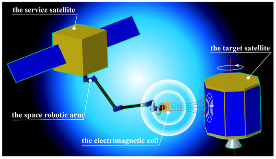
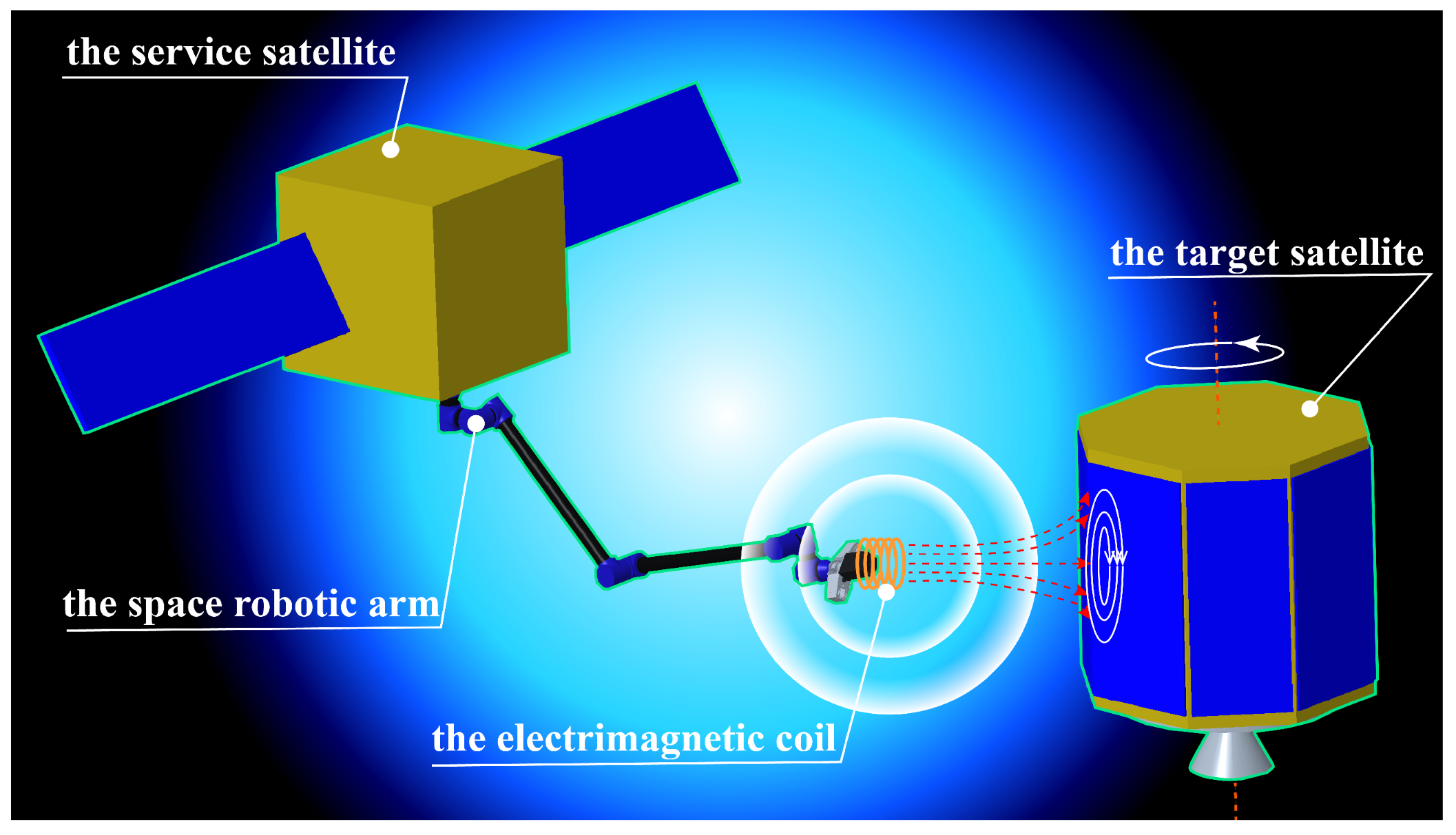
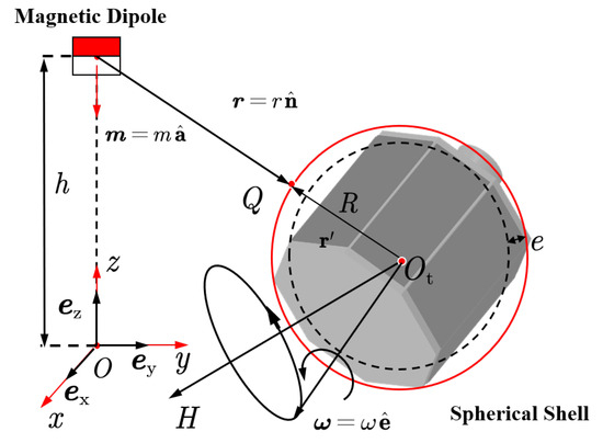
As illustrated in Figure 1, the electromagnetic de-tumbling system consists of a servicing spacecraft, a space manipulator, an electromagnetic coil mounted at the manipulator end-effector, and a non-cooperative target undergoing complex nutational motion at a general relative position.The satellite-like object shown in the mission-level schematic is not used as the computational geometry directly; instead, it is idealized as a homogeneous, non-magnetic conducting spherical shell for the analytical derivation and finite-element calculations in this study as shown in Figure 2.

Figure 1. Conceptual diagram of the electromagnetic de-tumbling system.

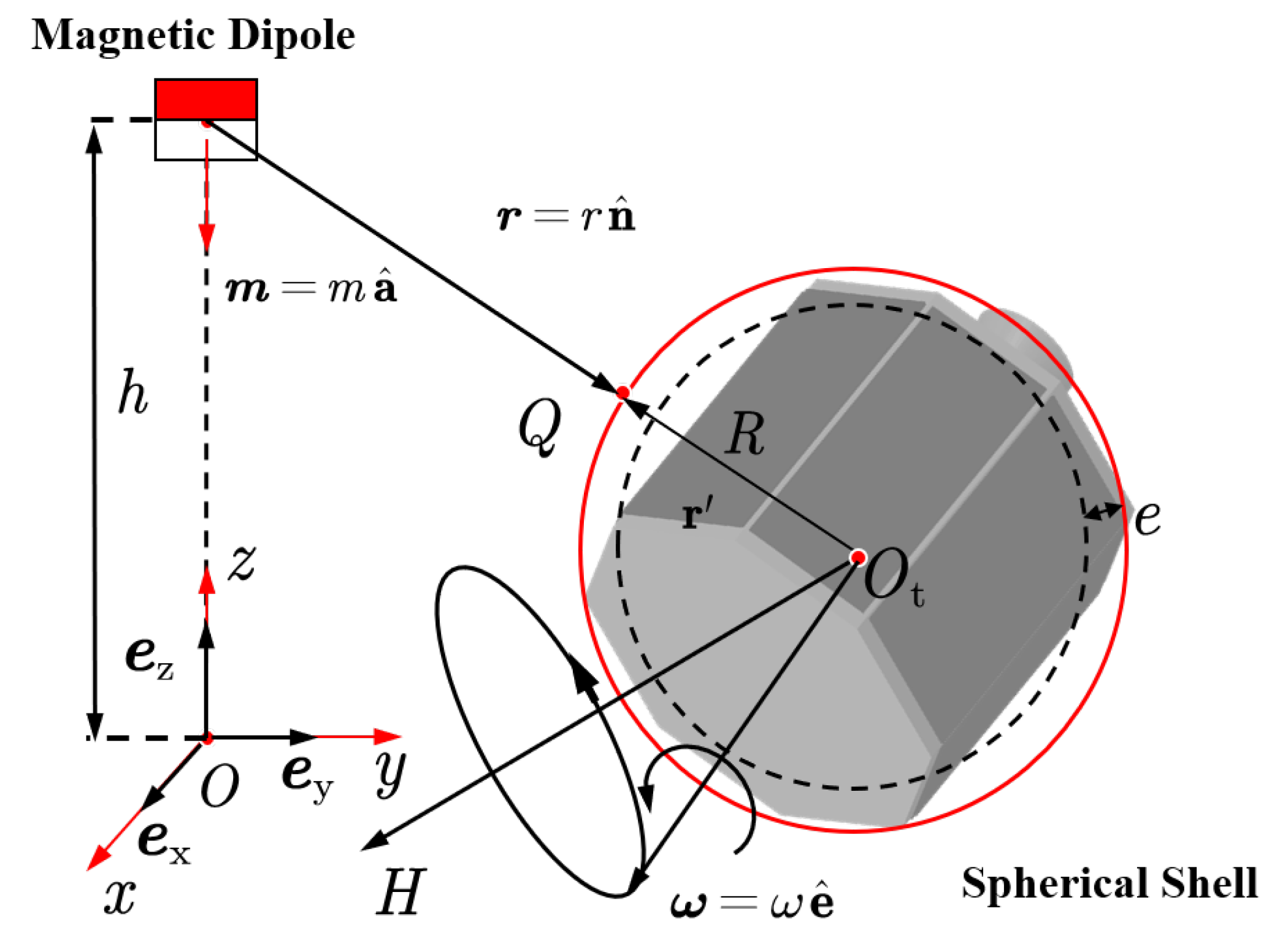
Figure 2. Conceptual diagram of the electromagnetic de-tumbling system and simplified illustration.

To make the subsequent analytical derivation tractable, three assumptions are introduced. First, the target is simplified as a non-magnetic, homogeneous conducting spherical shell, since such a sphere can serve as a first-order approximation of more complex conductive targets when the source–target separation is sufficiently large [31,33]. This approximation has been widely adopted in previous studies [24,31,32,33,37,39]. Second, because the relative distance between the magnetic dipole and the centroid of the spherical shell is much larger than the shell radius, the electromagnetic coil is approximated as a magnetic dipole [24,33]. Third, because the spatial variation of the dipole field over the shell surface is weak when the dipole–target separation is much larger than the shell radius, the magnetic flux density over the spherical shell is approximated by its value at the shell centroid, i.e., $\mathbf{B}\left(\mathbf{r}\right)\approx \mathbf{B}\left({\mathbf{r}}_t\right)$, so that the induced electromagnetic quantities can be derived in an approximate analytical form. The validity of the shell-center magnetic-field approximation is related to the distance-to-radius ratio $d/R$. Previous numerical–analytical comparisons showed that the torque error is already at the $0.1\%$ level when $d/R\approx 2.5$ and further decreases when $d/R\approx 3$ [24]. In this study, $d/R$ = 2.6–3.0 in the axial direction, and the bounded x- and y-offsets only increase the effective dipole-to-shell-center distance; thus, the distance-ratio condition is not weakened.

It should be noted that the spherical shell considered in this study is a canonical benchmark model rather than a direct representation of a specific debris object. The radius $R=0.1\mathrm{m}$ used in the numerical calculations is selected to provide a scaled geometry for finite-element validation and parameter fitting. Since the derived analytical expressions explicitly contain the geometric and physical parameters, including R, h, m, $\sigma$, and e, the formulation can be rescaled for larger conducting shells when the assumptions of the model remain valid. For real spacecraft with complex geometries, the present spherical-shell model should be regarded as a first-order reference model, and additional geometry-dependent correction is required.

As shown in Figure 2, a Cartesian inertial coordinate system $O-xyz$ is established with origin O and orthonormal basis vectors $({\mathbf{e}}_x,{\mathbf{e}}_y,{\mathbf{e}}_z)$. The non-cooperative target is modeled as a conducting spherical shell with outer radius R, thickness e, electrical conductivity $\sigma$, vacuum magnetic permeability ${\mu }_0$, and center $O_t$. The spherical shell undergoes nutational motion, with instantaneous angular velocity denoted by $\mathit{\omega }={\omega }_x{\mathbf{e}}_x+{\omega }_y{\mathbf{e}}_y+{\omega }_z{\mathbf{e}}_z=\omega \widehat{\mathbf{e}}$. The magnetic dipole moment is denoted by $\mathbf{m}=m\widehat{\mathbf{a}}$, where $\widehat{\mathbf{a}}=-{\mathbf{e}}_z$, and the dipole is located on the z-axis at a distance h from the origin. For an arbitrary point Q on the spherical shell surface, the position vector from the dipole to Q is denoted by $\mathbf{r}=r\widehat{\mathbf{n}}$. For later derivation, let ${\mathbf{r}}_t$ denote the position vector from the dipole to the shell center $O_t$, and let ${\mathbf{r}}^{\prime }$ denote the local position vector from $O_t$ to the surface point Q, so that $\mathbf{r}={\mathbf{r}}_t+{\mathbf{r}}^{\prime }$.

The magnetic flux density generated by the magnetic dipole at point Q on the spherical shell can be expressed as follows [40]:

$$\mathbf{B}\left(\mathbf{r}\right)={\displaystyle \frac{{\mu }_0}{4\pi }}\left(3\mathbf{m}·\left(\mathbf{r}\right){\displaystyle \frac{\mathbf{r}}{{\left|\mathbf{r}\right|}^5}}-{\displaystyle \frac{\mathbf{m}}{{\left|\mathbf{r}\right|}^3}}\right)$$

(1)

When the spherical shell moves in the magnetic field generated by the dipole, the induced eddy-current density in the shell can be described by Ohm’s law as:

$$\mathbf{j}=\sigma \left(-\nabla \phi +\mathbf{v}\times \mathbf{B}\right)$$

(2)

where $\phi$ denotes the induced electric potential, $\mathbf{B}$ is the primary magnetic field, and $\mathbf{v}$ represents the velocity of the spherical shell relative to the primary magnetic field.

The induced eddy current satisfies the charge-conservation law within the conducting volume.

$$\nabla ·\mathbf{j}=0$$

(3)

Since the induced eddy current is confined to the conducting spherical shell, the corresponding boundary condition is expressed as follows [38]:

$${\displaystyle \frac{\partial \phi }{\partial \mathbf{n}}}=\mathbf{n}·\left(\mathbf{v}\times \mathbf{B}\right)=0$$

(4)

Accordingly, the induced electric potential satisfies the Poisson equation.

$${\nabla }^2\phi =\nabla ·\left(\mathbf{v}\times \mathbf{B}\right)$$

(5)

The Lorentz force density acting on the spherical shell due to the external magnetic field is expressed as follows [39]:

$$\mathbf{f}=\mathbf{j}\times \mathbf{B}$$

(6)

The total electromagnetic force acting on the spherical shell is obtained by integrating the force density over the shell volume.

$$\mathbf{F}={\int }_V\mathbf{f}\mathrm{d}V={\int }_V\mathbf{j}\times \mathbf{B}\mathrm{d}V$$

(7)

where V is the volume of the spherical shell.

Similarly, the electromagnetic torque acting on the spherical shell is expressed as follows:

$$\mathbf{T}={\int }_V{\mathbf{r}}^{\prime }\times \mathbf{f}\mathrm{d}V={\int }_V{\mathbf{r}}^{\prime }\times \left(\mathbf{j}\times \mathbf{B}\right)\mathrm{d}V$$

(8)

3. Numerical Method for Electromagnetic Torque and Force

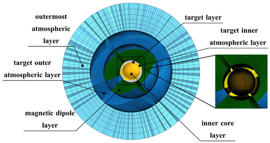
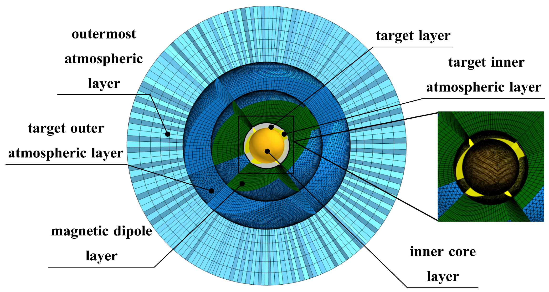
To achieve high numerical accuracy, improved computational efficiency, and robust convergence, a well-designed meshing strategy is essential. One effective approach is mesh parameterization, in which the magnetic field generated by the magnetic dipole is precomputed. This avoids direct meshing around the dipole singularity, significantly improves mesh quality, and reduces computational cost. In addition, the computational domain is divided into six layers, namely the outermost atmospheric layer, target outer atmospheric layer, magnetic dipole layer, target layer, target inner atmospheric layer, and inner core layer, as shown in Figure 3.

Figure 3. Demonstration of mesh grid layers for dipole-spherical shell model.

To ensure both rapid convergence and sufficient numerical accuracy, the radius of the outermost surrounding domain is set to six times that of the spherical shell. Since the magnetic field generated by the dipole is spatially open and decays gradually with distance, a sufficiently large surrounding air domain is required to avoid artificial truncation of the magnetic field near the target region. If the outer boundary is placed too close to the spherical shell, the imposed boundary condition may distort the local magnetic-field gradient, the induced eddy-current distribution, and consequently the calculated electromagnetic torque. Therefore, the enlarged outer domain is introduced to provide a stable far-field computational region while keeping the computational cost acceptable. The six-layer decomposition is used to separate the far-field air region, dipole region, shell region, and near-wall refinement region, so that different mesh densities can be assigned according to the local field and eddy-current variation. The mesh is further refined in the vicinity of the spherical shell because the eddy currents vary rapidly near its surface. The thickness and radius of each layer are listed in Table 1. By sweeping each layer to generate predominantly hexahedral elements, a high-quality mesh is obtained. The average mesh quality is 0.9095, where the mesh quality denotes the COMSOL-defined element quality index ranging from 0 to 1; a value closer to 1 indicates a more regular and less distorted element.

Table 1. Parameters used in numerical calculation.

Layer	Thickness (mm)	Radius (mm)	Grid Number
Outermost Atmospheric	240	600	104,652
Target Outer Atmospheric	120	360	156,978
Magnetic Dipole	140	240	156,978
Target	4	100	52,326
Target Inner Atmospheric	20	96	69,768
Inner Core	76	76	85,122

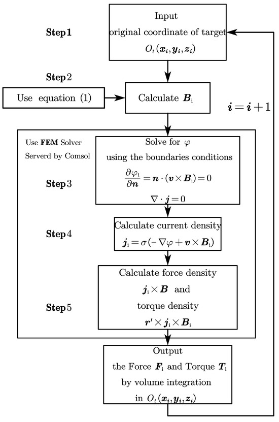
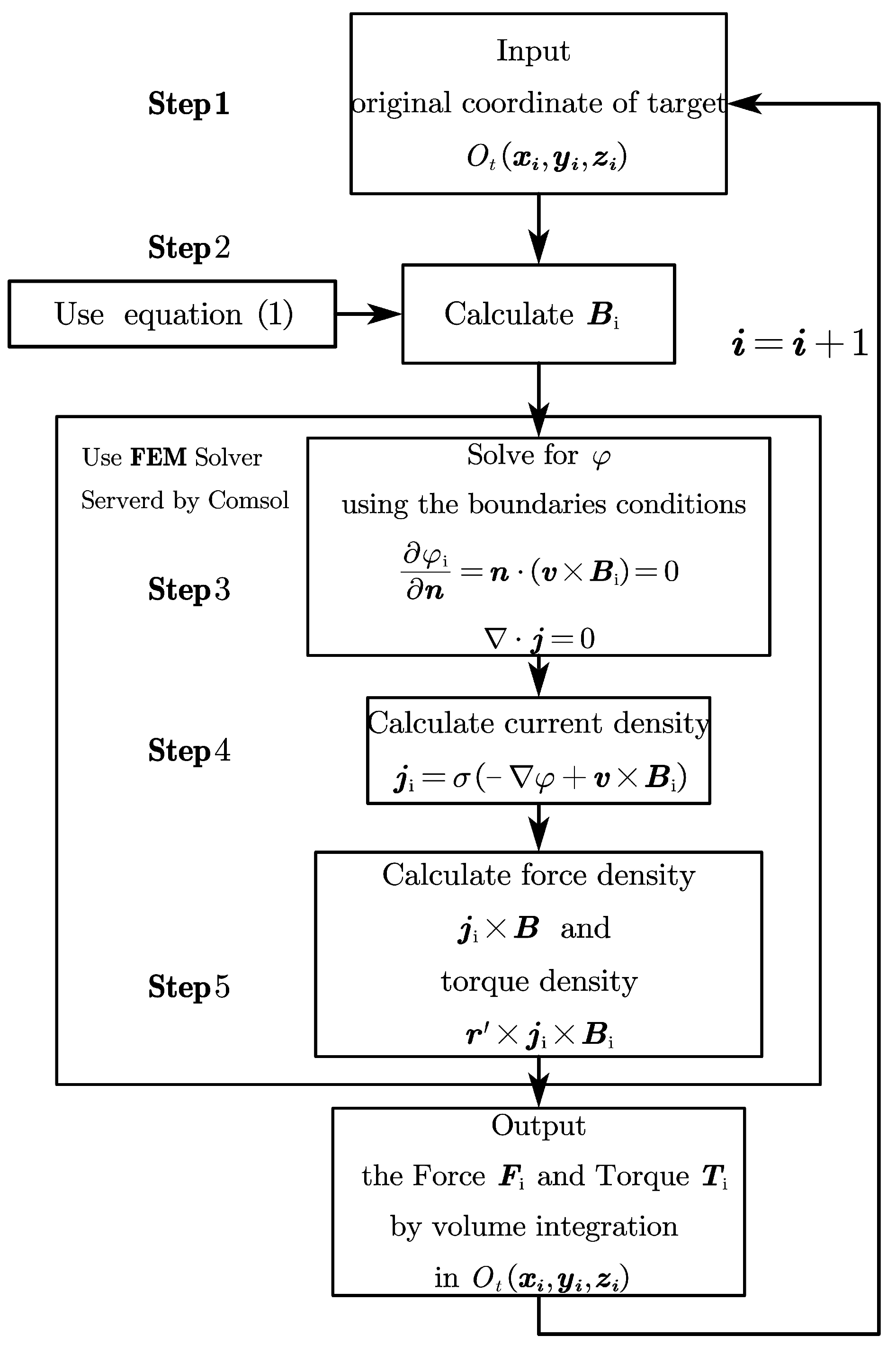
The position-dependent electromagnetic force and torque acting on the nutating spherical shell were systematically evaluated by finite element analysis, and the resulting numerical dataset was used as a benchmark solution set for the subsequent correction of the approximate analytical expressions. Assuming that the spherical-shell center was initially placed at the origin of the inertial coordinate system in COMSOL Multiphysics v.6.2, the electromagnetic force and torque at each sampling position were calculated according to the procedure shown in Figure 4.

Figure 4. Process for calculating the main parameters for the spherical shell in general position.

Step 1: Input the center coordinates of the spherical shell, namely $O_t(x_i,y_i,z_i)$.

Step 2: Using Equation (9), calculate the magnetic flux density at the shell center, denoted by ${\mathbf{B}}_i=\mathbf{B}\left({\mathbf{r}}_i\right)$,

$${\mathbf{B}}_i=\mathbf{B}\left({\mathbf{r}}_i\right)={\displaystyle \frac{{\mu }_0}{4\pi }}\left({\displaystyle \frac{3(\mathbf{m}·{\mathbf{r}}_i){\mathbf{r}}_i}{|{\mathbf{r}}_i{|}^5}}-{\displaystyle \frac{\mathbf{m}}{|{\mathbf{r}}_i{|}^3}}\right)$$

(9)

where ${\mathbf{r}}_i$ is the position vector from the magnetic dipole to the spherical-shell center.

For the nutating spherical shell, the rotational state at each instant is characterized by the angular velocity vector $\mathit{\omega }$. Accordingly, the local linear velocity of an arbitrary point Q in the shell can be written in the form $\mathbf{v}=\mathit{\omega }\times {\mathbf{r}}_i^{\prime }$, where ${\mathbf{r}}_i^{\prime }$ denotes the relative position vector from the shell center $O_t(x_i,y_i,z_i)$ to the point Q.

Step 3: In terms of charge conservation and the insulating boundary condition introduced above, the scalar electric potential ${\phi }_i$ can be solved in the finite element model.

Step 4: After ${\phi }_i$ is obtained, the eddy-current density can be calculated from Ohm’s law as follows:

$${\mathbf{j}}_i=\sigma \left[-\nabla {\phi }_i+\left(\mathit{\omega }\times {\mathbf{r}}_i^{\prime }\right)\times {\mathbf{B}}_i\right]$$

(10)

Step 5: The force density and torque density can then be expressed as ${\mathbf{j}}_i\times {\mathbf{B}}_i$ and ${\mathbf{r}}_i^{\prime }\times \left({\mathbf{j}}_i\times {\mathbf{B}}_i\right)$, respectively. Accordingly, the total electromagnetic force and torque at the sampled position can be obtained through volume integration as follows:

$${\mathbf{F}}_i={\int }_V{\mathbf{j}}_i\times {\mathbf{B}}_i\mathrm{d}V$$

(11)

$${\mathbf{T}}_i={\int }_V{\mathbf{r}}_i^{\prime }\times \left({\mathbf{j}}_i\times {\mathbf{B}}_i\right)\mathrm{d}V$$

(12)

By repeating the above procedure over all sampled positions, a benchmark database of position-dependent eddy-current forces and torques for the nutating spherical shell relative to the fixed magnetic dipole was established, which was subsequently used for the correction and validation of the approximate analytical expressions.

4. Numerical Results and Analysis

Finite element simulations were performed using the parameters given in Table 2. The spatial sampling domain was defined by $x,y\in [-0.04,0.04]\mathrm{m}$ with a step size of $0.01\mathrm{m}$, and $z\in [0.00,0.04]\mathrm{m}$ with the same step size, yielding 405 sampling points in total. At each sampling point, the electromagnetic torque vector acting on the nutating spherical shell in the magnetic dipole field was calculated.

Table 2. Finite element simulation parameter table.

Parameter	Value
Magnetic Dipole Moment (m)	$500\mathrm{A}·{\mathrm{m}}^2$
Dipole-to-Shell Distance (h)	0.3 $\mathrm{m}$
Electrical Conductivity ($\sigma$)	$3.7\times {10}^7$$\mathrm{S}/\mathrm{m}$
Vacuum Permeability (${\mu }_0$)	$4\pi \times {10}^{-7}$$\mathrm{T}·\mathrm{m}/\mathrm{A}$
Spherical Shell Thickness (e)	$0.004\mathrm{m}$
Angular Velocity ($\omega$)	${[8,1.6,1.6]}^{\mathrm{T}}\mathrm{deg}/\mathrm{s}$
Shell Radius (R)	0.1 $\mathrm{m}$

Note: The shell radius $R=0.1\mathrm{m}$ is selected as a scaled benchmark geometry for analytical-model derivation and finite-element validation. It should not be interpreted as the size of a specific debris object intended for robotic-arm capture in an actual mission.

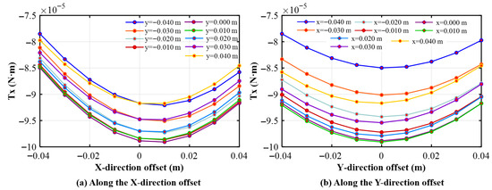
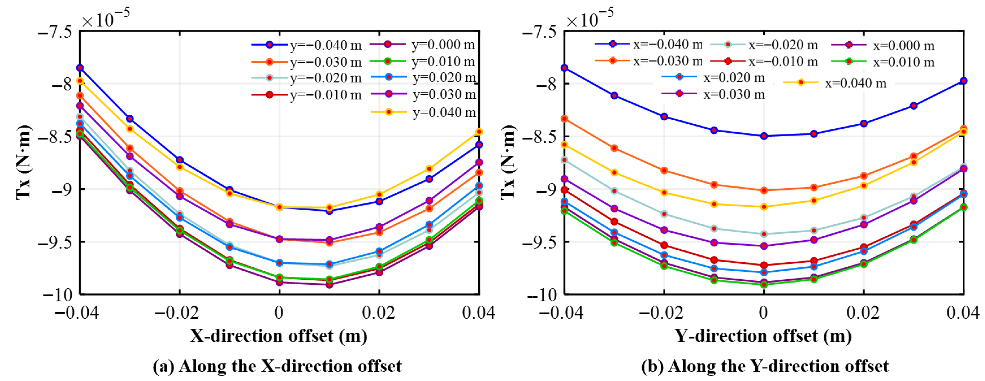
Since the torque distributions on the five section planes from $z=0.00$ to $z=0.04\mathrm{m}$ exhibit similar overall patterns in the $xy$ plane, the plane $z=0.00\mathrm{m}$ is selected here as the representative section for detailed analysis. On this plane, the electromagnetic torque on the nutating spherical shell contains three components, $T_x$, $T_y$, and $T_z$, whose average absolute magnitudes are about $9.16\times {10}^{-5}$, $1.83\times {10}^{-5}$, and $9.51\times {10}^{-6}\mathrm{N}·\mathrm{m}$, respectively. Accordingly, $T_x$ is the dominant component, being about 5 times $T_y$ and about 10 times $T_z$, while $T_y$ is about 2 times $T_z$; however, since all three components remain at the same order of magnitude, namely ${10}^{-5}\mathrm{N}·\mathrm{m}$, the secondary components $T_y$ and $T_z$ cannot be neglected and should also be included in the subsequent calculation and correction of the analytical model.

As shown in Figure 5a, under fixed y-offset conditions, the braking torque magnitude of the $T_x$ component first increases and then decreases as the shell center moves along the x direction. As x varies from $-0.04$ toward the central region, the braking effect strengthens rapidly, whereas after passing the strongest braking region it weakens gradually toward $x=0.04\mathrm{m}$. Moreover, the increment of the braking torque magnitude on the negative-x side decreases progressively, indicating that the sensitivity of $T_x$ to the x-offset weakens near the central region. Over the whole plane, the strongest braking torque appears at $(x,y)=(0.00,0.01)\mathrm{m}$, where $|T_x|=9.9078\times {10}^{-5}\mathrm{N}·\mathrm{m}$. In addition, the two branches on the negative-x and positive-x sides are unequal, and the braking torque near $x=0.04\mathrm{m}$ is generally larger than that near $x=-0.04\mathrm{m}$, confirming the asymmetric distribution of $T_x$ along the x direction.

Figure 5. Distribution of the $T_x$ electromagnetic torque in the plane $z=0.00\mathrm{m}$.

As shown in Figure 5b, under fixed x-offset conditions, the braking torque magnitude of the $T_x$ component also first increases and then decreases as the shell center moves along the y direction. The strongest braking region is concentrated near the central neighborhood and is shifted slightly toward the positive-y side. Compared with the positive-y branch, the increase in braking torque magnitude from $y=-0.04\mathrm{m}$ toward the strongest braking region is steeper, indicating a higher sensitivity of $T_x$ to the y-offset on the negative-y side. For example, when $x=0.00\mathrm{m}$, the braking torque magnitude increases from $8.9043\times {10}^{-5}$ at $y=-0.04\mathrm{m}$ to the plane maximum $9.9078\times {10}^{-5}\mathrm{N}·\mathrm{m}$ at $y=0.01\mathrm{m}$, and then decreases to $8.8081\times {10}^{-5}\mathrm{N}·\mathrm{m}$ at $y=0.04\mathrm{m}$. Therefore, the $T_x$ distribution is asymmetric in both the x and y directions, and its strongest braking region is slightly shifted from the geometric center of the section plane. The slight shift of the strongest braking region is attributed to the coupling between the nutational angular-velocity components and the nonuniform dipole field. Although the dipole field is axisymmetric about the z-axis, the nonzero ${\omega }_y$ and ${\omega }_z$ components modify the local velocity field $\mathbf{v}=\mathit{\omega }\times {\mathbf{r}}^{\prime }$, thereby changing the local eddy-current and Lorentz-force distributions. Since the torque depends on both the Lorentz force and its moment arm, this weak in-plane asymmetry shifts the maximum $T_x$ braking region slightly away from the geometric center.

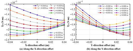
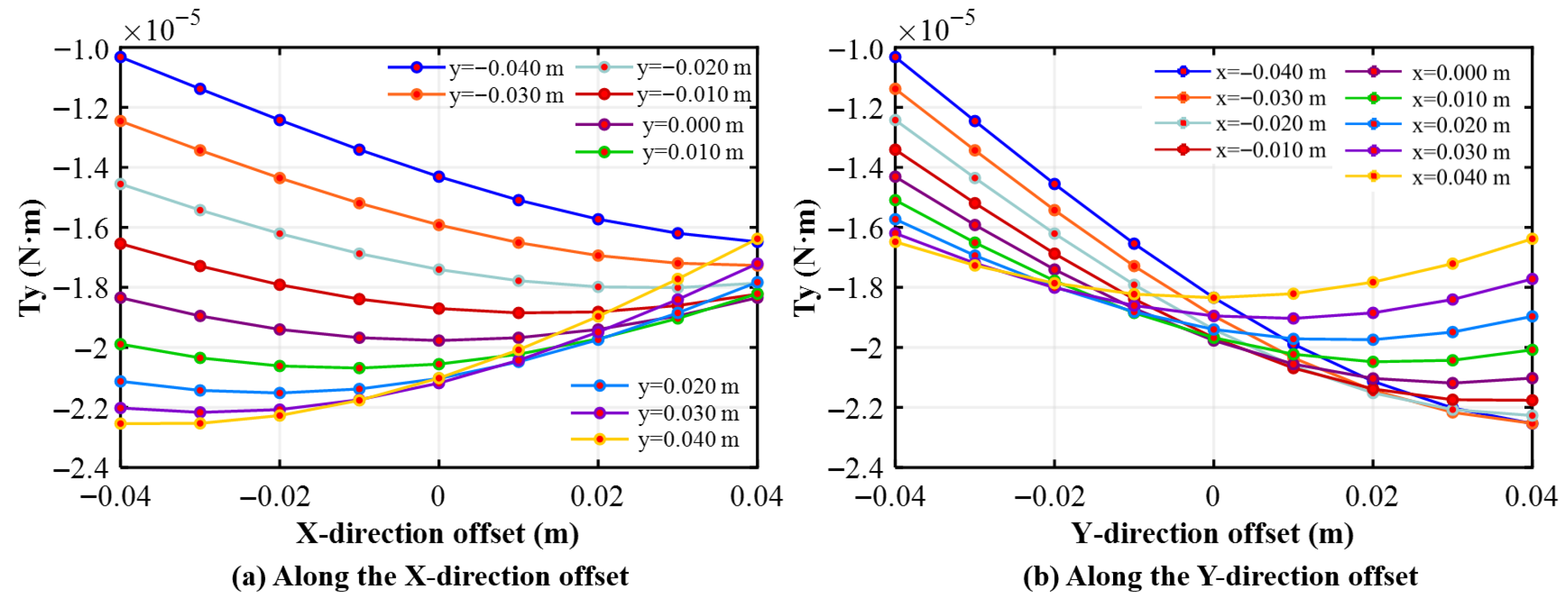
As shown in Figure 6a, under fixed y-offset conditions, the braking torque magnitude of the $T_y$ component exhibits a strongly coupled and non-uniform distribution along the x direction. For negative y-offsets, $|T_y|$ generally increases as x varies from $-0.04$ to $0.04\mathrm{m}$, and the strongest braking torque appears near the positive end of the sampled x-range. However, as y increases toward the positive side, the monotonic trend gradually weakens, the location of the strongest braking region shifts continuously, and the curves become distinctly non-monotonic. In particular, for sufficiently large positive y-offsets, the strongest braking region is no longer located near the positive-x side, but moves toward the negative-x side. Therefore, the extrema of the $T_y$ component do not remain at a fixed x position, and the variation rate of the torque is also evidently non-uniform, indicating a much stronger two-dimensional coupling than that observed for the dominant $T_x$ component.

Figure 6. Distribution of the $T_y$ electromagnetic torque in the plane $z=0.00\mathrm{m}$.

As shown in Figure 6b, under fixed x-offset conditions, the braking torque magnitude of the $T_y$ component exhibits a clear migration of its strongest braking region along the y direction. For negative x-offsets, the strongest braking torque appears near the positive-y side; for x close to zero, it is located near the central region; and for positive x-offsets, it shifts further toward the negative-y side. In other words, the extrema of the $T_y$ component move continuously across the sampled y-range as the shell center shifts along the x direction. Moreover, the curve shapes and the corresponding variation rates differ evidently for different fixed x values, which further indicates that the $T_y$ component is governed by a pronounced two-dimensional coupling in the $xy$ plane. Although $T_y$ is a secondary torque component, its magnitude relative to the dominant $T_x$ component remains non-negligible; therefore, it should also be retained in the subsequent analytical calculation and correction.

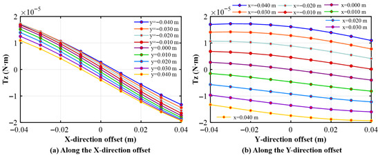
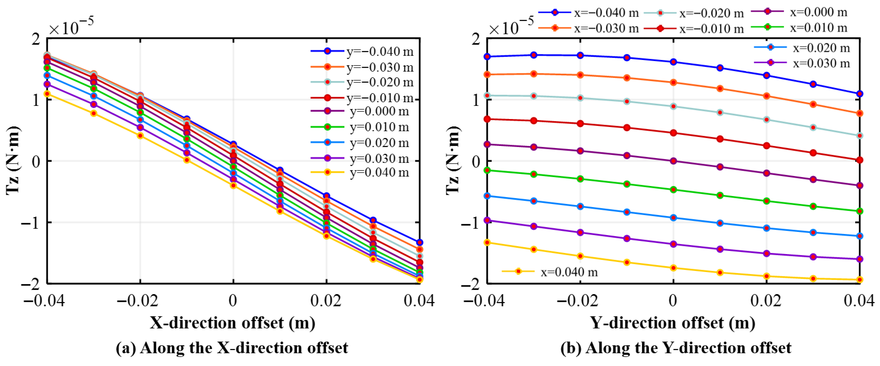
As shown in Figure 7a, under fixed y-offset conditions, the $T_z$ component exhibits a clear transition from acceleration torque to braking torque as the shell center moves along the x direction. In the negative-x region, $T_z$ is generally positive, which means that the electromagnetic torque tends to accelerate the rotational motion and is therefore unfavorable for de-tumbling. As x increases, $T_z$ decreases continuously, gradually crosses zero near the central region, and then becomes negative in the positive-x region, indicating that the torque changes into a braking torque and begins to contribute to angular-velocity decay. Over the whole section plane, the largest positive $T_z$ appears at $(x,y)=(-0.03,-0.04)\mathrm{m}$, where $T_z=1.7262\times {10}^{-5}\mathrm{N}·\mathrm{m}$, whereas the largest negative $T_z$, corresponding to the strongest braking effect, appears at $(x,y)=(0.04,0.04)\mathrm{m}$, where $T_z=-1.9338\times {10}^{-5}\mathrm{N}·\mathrm{m}$. In addition, the variation rate of $T_z$ along the x direction is evidently non-uniform: in the negative-x side the change is relatively slow, whereas after approaching the central region the decreasing rate becomes progressively larger toward the positive-x side. This indicates that the $T_z$ component is more sensitive to the x-offset in the positive-x region, where a small position change may produce a more significant variation in the braking torque. Meanwhile, on the representative plane $z=0.00\mathrm{m}$, the average magnitude of $T_z$ is only about one-tenth of that of the dominant $T_x$ component, and even its maximum magnitude is only about one-fifth of the maximum $|T_x|$. Therefore, although the positive-$T_z$ region locally tends to accelerate the rotational motion, this effect does not dominate the overall de-tumbling behavior, because the braking action is still primarily governed by the dominant $T_x$ component.

Figure 7. Distribution of the $T_z$ electromagnetic torque in the plane $z=0.00\mathrm{m}$.

As shown in Figure 7b, under fixed x-offset conditions, the $T_z$ component generally decreases as the shell center moves along the y direction from $-0.04$ to $0.04\mathrm{m}$. For negative-x curves, $T_z$ crosses zero near the central region, indicating a transition from accelerating torque to braking torque, whereas for positive-x curves it remains negative throughout the sampled range and therefore always contributes to rotational deceleration. In addition, the decreasing rate is evidently non-uniform, being larger near the central region and smaller near the two ends of the sampled y-range.

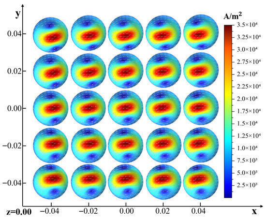
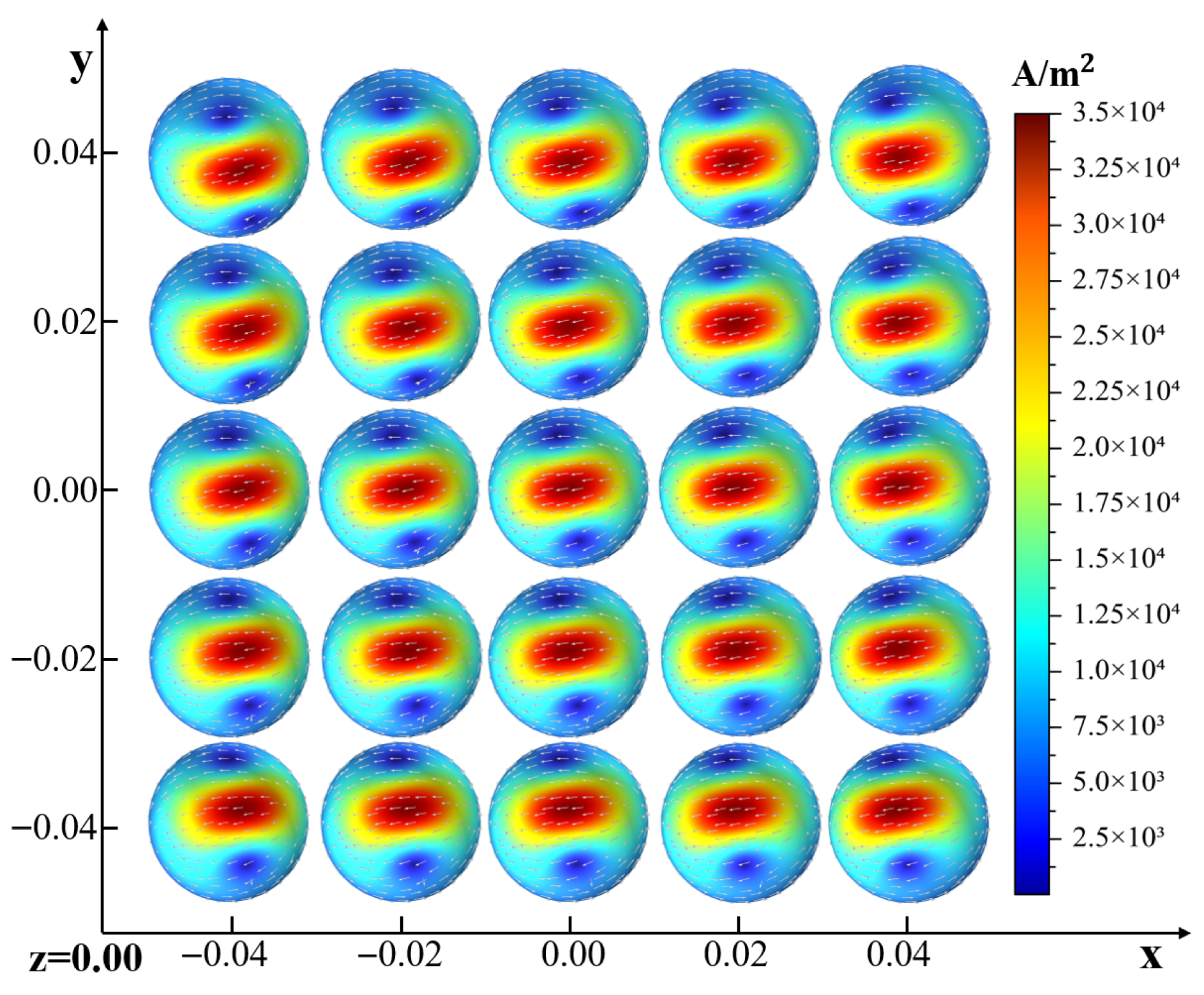
As shown in Figure 8, the surface eddy-current density distributions of the spherical shell at the sampled positions in the plane $z=0.00\mathrm{m}$ present a similar overall topology. The induced eddy current forms a closed-loop pattern on the shell surface for all sampled positions, with the high-current-density region concentrated in an oblique belt-like zone and the low-current-density regions distributed near the two opposite sides of the shell. Although the shell center changes in the $xy$ plane, the loop morphology remains nearly unchanged, whereas the local intensity and gradient of the current density vary with position. The peak eddy-current density remains in the order of ${10}^4\mathrm{A}/{\mathrm{m}}^2$, with a maximum close to $3.5\times {10}^4\mathrm{A}/{\mathrm{m}}^2$. This indicates that bounded in-plane offsets do not alter the fundamental induction pattern, but they do modulate the local current-density distribution and thereby affect the electromagnetic torque acting on the spherical shell.

Figure 8. Surface eddy-current density distributions of the spherical shell at sampled positions in the plane $z=0.00\mathrm{m}$.

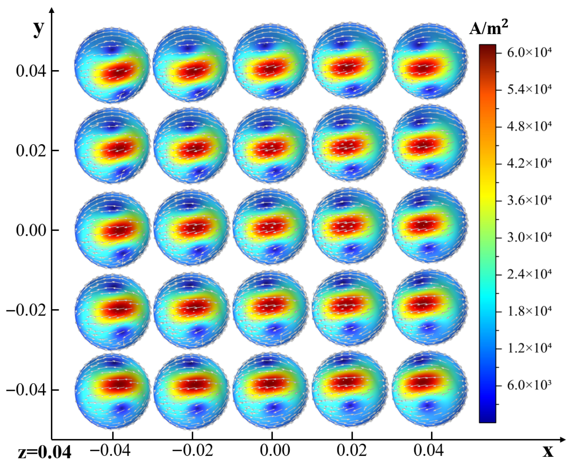
As shown in Figure 9, the surface eddy-current density distribution of the spherical shell in the plane $z=0.04\mathrm{m}$ is highly similar to that in the plane $z=0.00\mathrm{m}$. The induced eddy current still exhibits a nearly identical closed-loop topology, with the high-current-density region concentrated in an oblique belt-like zone. The main difference lies in the current-density magnitude, which is significantly enhanced at $z=0.04\mathrm{m}$. According to the color scale, the peak eddy-current density increases from about $3.5\times {10}^4$ to $6.0\times {10}^4\mathrm{A}/{\mathrm{m}}^2$, indicating that the electromagnetic induction effect becomes substantially stronger as the spherical shell moves closer to the magnetic dipole.

Figure 9. Surface eddy-current density distributions of the spherical shell at sampled positions in the plane $z=0.04\mathrm{m}$.

The similarity of the eddy-current distributions in Figure 8 and Figure 9 refers only to the overall closed-loop topology. The local current-density magnitude, gradient, and high-current-density region still vary with the shell-center position. Since the electromagnetic torque is determined by ${\int }_V{\mathbf{r}}^{\prime }\times (\mathbf{j}\times \mathbf{B})\mathrm{d}V$, changes in the local Lorentz force density, current-density centroid, and moment arm can still produce significant position-dependent torque variations even when the global current-loop pattern remains similar.

5. Derivation and Fitting of Approximate Analytical Expressions for Electromagnetic Torque

5.1. Approximate Analytical Derivation of Electromagnetic Torque

To derive an approximate analytical expression for the electromagnetic torque acting on the nutating spherical shell, the magnetic field over the shell surface is approximated by the magnetic flux density at the shell center. This approximation is valid when the relative distance between the magnetic dipole and the spherical shell is much larger than the shell radius. Accordingly, the magnetic field used in the following derivation is written as $\mathbf{B}\left({\mathbf{r}}_{\mathrm{t}}\right)$, where ${\mathbf{r}}_{\mathrm{t}}=x{\mathbf{e}}_x+y{\mathbf{e}}_y+(z-h){\mathbf{e}}_z$ denotes the position vector from the magnetic dipole to the shell center, and $r_{\mathrm{t}}=\left|{\mathbf{r}}_{\mathrm{t}}\right|=\sqrt{x^2+y^2+{(z-h)}^2}$ is the corresponding distance. For brevity, the unit vector from the magnetic dipole to the shell center is still denoted by $\widehat{\mathbf{n}}$ in this subsection, namely, $\widehat{\mathbf{n}}={\mathbf{r}}_{\mathrm{t}}/r_{\mathrm{t}}$. Meanwhile, $\widehat{\mathbf{a}}=-{\mathbf{e}}_z$ denotes the unit vector of the magnetic dipole moment direction, and $\omega =\omega \widehat{\mathbf{e}}$ denotes the instantaneous angular velocity vector of the nutating spherical shell. Throughout this subsection, x, y, z, h, R, and e are expressed in $\mathrm{m}$, the angular-velocity components are expressed in $\mathrm{rad}/\mathrm{s}$, and the torque components are obtained in $\mathrm{N}·\mathrm{m}$.

With the above definitions, the magnetic flux density at the shell center can be rewritten in unit-vector form as follows:

$$\mathbf{B}\left({\mathbf{r}}_{\mathrm{t}}\right)={\displaystyle \frac{{\mu }_{0}m}{4\pi r_{\mathrm{t}}^3}}\left[3\left(\widehat{\mathbf{a}}·\widehat{\mathbf{n}}\right)\widehat{\mathbf{n}}-\widehat{\mathbf{a}}\right]$$

(13)

Under the thin-shell approximation, the induced magnetic moment of the conducting spherical shell can be expressed as [40]:

$${\mathbf{m}}_{\mathrm{s}}={\displaystyle \frac{4\pi }{15}}\sigma e{R}^5\left(\mathit{\omega }\times \mathbf{B}\left({\mathbf{r}}_{\mathrm{t}}\right)\right)$$

(14)

For the present low-speed condition, the skin effect can be neglected. The magnitude of the initial angular velocity is $|{\mathit{\omega }}_0|=8.31\mathrm{deg}/\mathrm{s}=0.145\mathrm{rad}/\mathrm{s}$. Substituting this value into the skin-depth expression $\delta =\sqrt{2/\left({\mu }_0\sigma \right|{\mathit{\omega }}_0\left|\right)}$ gives $\delta \approx 0.54\mathrm{m}$. Since the shell thickness is $e=0.004\mathrm{m}$, $\delta /e\approx 135\gg 1$, indicating sufficient magnetic-field penetration through the shell thickness. This is consistent with the low-speed assumptions in Youngquist et al. [37] and Yu et al. [24], where the eddy-current-induced secondary magnetic field is assumed to be much smaller than the applied field.

Accordingly, the electromagnetic torque acting on the spherical shell is written as:

$${\mathbf{T}}_{\mathrm{s}}={\mathbf{m}}_{\mathrm{s}}\times \mathbf{B}\left({\mathbf{r}}_{\mathrm{t}}\right)$$

(15)

Substituting Equation (14) into Equation (15) yields

$${\mathbf{T}}_{\mathrm{s}}={\displaystyle \frac{4\pi }{15}}\sigma e{R}^5\left[\left(\mathit{\omega }\times \mathbf{B}\left({\mathbf{r}}_{\mathrm{t}}\right)\right)\times \mathbf{B}\left({\mathbf{r}}_{\mathrm{t}}\right)\right]$$

(16)

Using the vector identity $(\mathit{\omega }\times \mathbf{B})\times \mathbf{B}=(\mathit{\omega }·\mathbf{B})\mathbf{B}-{\left|\mathbf{B}\right|}^2\mathit{\omega }$, Equation (16) can be rewritten as:

$${\mathbf{T}}_{\mathrm{s}}={\displaystyle \frac{4\pi }{15}}\sigma e{R}^5\left[\left(\mathit{\omega }·\mathbf{B}\left({\mathbf{r}}_{\mathrm{t}}\right)\right)\mathbf{B}\left({\mathbf{r}}_{\mathrm{t}}\right)-{\left|\mathbf{B}\left({\mathbf{r}}_{\mathrm{t}}\right)\right|}^2\mathit{\omega }\right]$$

(17)

By substituting Equation (13) into Equation (17), the approximate analytical electromagnetic torque can be written in the following compact vector form:

$$\begin{array}{cc}{\mathbf{T}}_{\mathrm{s}}={\displaystyle \frac{{\mu }_0^2{m}^2\sigma e{R}^5}{60\pi r_{\mathrm{t}}^6}}[\hfill & \widehat{\mathbf{n}}\left(9{(\widehat{\mathbf{a}}·\widehat{\mathbf{n}})}^2(\mathit{\omega }·\widehat{\mathbf{n}})-3(\widehat{\mathbf{a}}·\widehat{\mathbf{n}})(\mathit{\omega }·\widehat{\mathbf{a}})\right)\hfill \\ \hfill & +\widehat{\mathbf{a}}\left((\mathit{\omega }·\widehat{\mathbf{a}})-3(\widehat{\mathbf{a}}·\widehat{\mathbf{n}})(\mathit{\omega }·\widehat{\mathbf{n}})\right)+\mathit{\omega }\left(-3{(\widehat{\mathbf{a}}·\widehat{\mathbf{n}})}^2-1\right)]\hfill \end{array}$$

(18)

For the present configuration, $\widehat{\mathbf{a}}·\widehat{\mathbf{n}}=-(z-h)/r_{\mathrm{t}}$ and $\mathit{\omega }·\widehat{\mathbf{a}}=-{\omega }_z$. Meanwhile, $\mathit{\omega }·\widehat{\mathbf{n}}=\left({\omega }_{x}x+{\omega }_{y}y+{\omega }_z(z-h)\right)/r_{\mathrm{t}}$.

For brevity, let $\chi =\mathit{\omega }·{\mathbf{r}}_{\mathrm{t}}={\omega }_{x}x+{\omega }_{y}y+{\omega }_z(z-h)$. Then, the three components of the approximate analytical electromagnetic torque can be obtained as follows:

$$T_x={\displaystyle \frac{{\mu }_0^2{m}^2\sigma e{R}^5}{60\pi r_{\mathrm{t}}^9}}\left[9x{(z-h)}^2\chi -3x(z-h){\omega }_z{r}_{\mathrm{t}}^2-{\omega }_x{r}_{\mathrm{t}}^2\left(3{(z-h)}^2+r_{\mathrm{t}}^2\right)\right]$$

(19)

$$T_y={\displaystyle \frac{{\mu }_0^2{m}^2\sigma e{R}^5}{60\pi r_{\mathrm{t}}^9}}\left[9y{(z-h)}^2\chi -3y(z-h){\omega }_z{r}_{\mathrm{t}}^2-{\omega }_y{r}_{\mathrm{t}}^2\left(3{(z-h)}^2+r_{\mathrm{t}}^2\right)\right]$$

(20)

$$T_z={\displaystyle \frac{{\mu }_0^2{m}^2\sigma e{R}^5}{60\pi r_{\mathrm{t}}^9}}\left[9{(z-h)}^3\chi -3{(z-h)}^2{\omega }_z{r}_{\mathrm{t}}^2+3(z-h)r_{\mathrm{t}}^2\chi -{\omega }_z{r}_{\mathrm{t}}^4\right]$$

(21)

Therefore, the uncorrected approximate analytical expression for the electromagnetic torque acting on the nutating spherical shell in the magnetic dipole field can be summarized as ${\mathbf{T}}_{\mathrm{s}}={[T_x,T_y,T_z]}^{\mathrm{T}}$.

5.2. Fitting of Approximate Analytical Expressions for Electromagnetic Torque

Although the approximate analytical torque model derived above captures the primary dependence of the electromagnetic torque on the relative position and angular velocity, systematic deviations still exist between the analytical predictions and the finite-element results. To improve the prediction accuracy while retaining a compact analytical form, correction terms are introduced for the three torque components.

The corrected model is constructed by combining a theoretical leading term with a data-fitted polynomial compensation term. The theoretical leading term is obtained from the magnetic-dipole/spherical-shell analytical model and preserves the main physical dependence of the torque on position and angular velocity. The polynomial term is used to compensate for the residual spatial deviation from the finite-element benchmark within the bounded offset domain. Considering both fitting accuracy and model compactness, a second-order polynomial correction is adopted for the dominant $T_x$ component, whereas third-order polynomial corrections are adopted for the secondary $T_y$ and $T_z$ components.

Accordingly, the corrected analytical expression of the $T_x$ component is written as:

$$T_x^{\mathrm{c}}={\alpha }_x{T}_x+c_{x1}x+c_{x2}y+c_{x3}xy+c_{x4}{x}^2+c_{x5}{y}^2$$

(22)

where ${\alpha }_x$ is an amplitude scaling coefficient of the theoretical leading term, obtained by fitting to the finite-element torque data. It compensates for the systematic magnitude deviation between the uncorrected analytical expression and the finite-element benchmark, while $c_{x1}$–$c_{x5}$ describe the residual spatial correction in the bounded offset domain.

Similarly, the corrected analytical expression of the $T_y$ component is written as

$$\begin{array}{cc}{T}_y^{\mathrm{c}}={\alpha }_y{T}_y\hfill & +c_{y1}x+c_{y2}y+c_{y3}xy+c_{y4}{x}^2+c_{y5}{y}^2\hfill \\ \hfill & +c_{y6}{x}^3+c_{y7}{y}^3+c_{y8}{x}^{2}y+c_{y9}x{y}^2\hfill \end{array}$$

(23)

where ${\alpha }_y$ is the amplitude scaling coefficient of the theoretical leading term, and $c_{y1}$–$c_{y9}$ are the polynomial coefficients used to compensate for residual spatial deviations.

For the $T_z$ component, the corrected analytical expression is written as

$$\begin{array}{cc}{T}_z^{\mathrm{c}}={\alpha }_z{T}_z\hfill & +c_{z1}x+c_{z2}y+c_{z3}xy+c_{z4}{x}^2+c_{z5}{y}^2\hfill \\ \hfill & +c_{z6}{x}^3+c_{z7}{y}^3+c_{z8}{x}^{2}y+c_{z9}x{y}^2\hfill \end{array}$$

(24)

where ${\alpha }_z$ is the amplitude scaling coefficient of the theoretical leading term, and $c_{z1}$–$c_{z9}$ are the polynomial coefficients used to compensate for residual spatial deviations.

Accordingly, the corrected approximate analytical torque model can be summarized in vector form as ${\mathbf{T}}_{\mathrm{s}}^{\mathrm{c}}={[T_x^{\mathrm{c}},T_y^{\mathrm{c}},T_z^{\mathrm{c}}]}^{\mathrm{T}}$.

The relatively large error of the uncorrected analytical model mainly reflects a systematic amplitude deviation rather than an incorrect torque-distribution trend. The leading analytical expressions preserve the primary dependence of the electromagnetic torque on the relative position and angular velocity. However, due to the shell-center magnetic-field approximation, the equivalent induced-moment approximation, and the neglect of higher-order spatial coupling terms, the torque amplitude is not fully consistent with the finite-element benchmark. Since the electromagnetic torque is highly sensitive to the dipole-to-shell distance, this amplitude mismatch can lead to a large relative error. Therefore, the scaling factors in Equations (22)–(24) are introduced mainly to compensate for the systematic amplitude deviation, while the low-order polynomial terms correct the remaining position-dependent residual deviations within the bounded offset domain.

The correction coefficients in Equations (22)–(24) are calibration parameters for the present spherical-shell benchmark model within the bounded offset domain, rather than universal constants. The theoretical leading terms retain the dominant scaling with m, $\sigma$, e, R, and the dipole-to-shell distance. Thus, changes in m, $\sigma$, or e mainly affect the torque amplitude through the leading term, whereas changes in the shell radius, distance-to-radius ratio, target geometry, or calibrated spatial domain may require recalibration of the correction coefficients. For control-oriented applications, such calibration can be performed offline, while the corrected analytical expressions can be evaluated rapidly online.

The unknown coefficients are determined by nonlinear least-squares fitting based on the finite-element torque data obtained. To quantitatively evaluate the corrected analytical model, two relative-error indices are introduced. The first is the local average relative error ${\epsilon }_1$, which evaluates the average fitting error along the x direction at a fixed y position. It is defined as

$${\epsilon }_1\left(y_j\right)={\displaystyle \frac{1}{N_x}}{\displaystyle \sum _{i=1}^{N_x}}{\displaystyle \frac{\left|T_{\mathrm{a}}(x_i,y_j)-T_{\mathrm{n}}(x_i,y_j)\right|}{\left|T_{\mathrm{n}}(x_i,y_j)\right|}}$$

(25)

where $N_x=9$ is the number of sampling points in the x direction, $T_{\mathrm{a}}(x_i,y_j)$ denotes the analytical value obtained from either the corrected or the uncorrected model, and $T_{\mathrm{n}}(x_i,y_j)$ denotes the corresponding finite-element result. This index is used to evaluate the line-wise fitting accuracy at different fixed y offsets.

The second is the global average relative error ${\epsilon }_2$, which evaluates the overall fitting error over the whole sampled plane. It is defined as

$${\epsilon }_2={\displaystyle \frac{1}{N_y{N}_x}}{\displaystyle \sum _{j=1}^{N_y}}{\displaystyle \sum _{i=1}^{N_x}}{\displaystyle \frac{\left|T_{\mathrm{a}}(x_i,y_j)-T_{\mathrm{n}}(x_i,y_j)\right|}{\left|T_{\mathrm{n}}(x_i,y_j)\right|}}$$

(26)

where $N_x=9$ and $N_y=9$ are the numbers of sampling points in the x and y directions, respectively. This index is used to evaluate the overall agreement between the corrected analytical model and the finite-element results over the entire sampled domain.

With the above fitting strategy, the corrected analytical model preserves the physical structure of the original approximate torque expression while introducing only low-order polynomial compensation terms. This makes it possible to substantially improve the computational accuracy without losing the analytical compactness required for subsequent dynamic analysis and control-oriented applications.

5.3. Identification and Analysis of the Fitted Correction Coefficients

The polynomial correction terms are used only as local compensation terms and do not change the primary functional trend of the analytical model. For the corrected $T_x$ component, the fitted scaling factor is ${\alpha }_x=138.6317$, and the polynomial correction coefficients are $c_{x1}=8.9304\times {10}^{-5}$, $c_{x2}=-8.2699\times {10}^{-5}$, $c_{x3}=-3.5145\times {10}^{-5}$, $c_{x4}=-1.3286\times {10}^{-3}$, and $c_{x5}=3.0587\times {10}^{-3}$. It can be seen that the second-order terms, especially $c_{x4}$ and $c_{x5}$, are clearly larger than the linear and bilinear terms, indicating that the correction of $T_x$ is dominated by low-order polynomial compensation rather than by higher-order coupling. At the same time, although the quadratic coefficients are larger than the other correction coefficients, they are still small in absolute magnitude, and their actual contribution remains limited within the bounded offset domain. This indicates that the original analytical expression already captures the correct physical form and main variation trend of $T_x$, while the correction mainly compensates for the amplitude deviation and the local curvature error.

For the corrected $T_y$ component, the fitted scaling factor is ${\alpha }_y=138.6331$, and the polynomial correction coefficients are $c_{y1}=-9.2601\times {10}^{-5}$, $c_{y2}=9.8337\times {10}^{-5}$, $c_{y3}=-1.7535\times {10}^{-4}$, $c_{y4}=6.1176\times {10}^{-4}$, $c_{y5}=-2.6562\times {10}^{-4}$, $c_{y6}=5.4058\times {10}^{-3}$, $c_{y7}=-4.9251\times {10}^{-3}$, $c_{y8}=-4.8319\times {10}^{-3}$, and $c_{y9}=5.2823\times {10}^{-3}$. The third-order coefficients are evidently larger than the linear and quadratic ones, indicating that the correction of $T_y$ is mainly governed by higher-order terms. Nevertheless, the overall magnitudes of these fitted coefficients remain limited, which means that the original theoretical expression of $T_y$ remains physically valid and only requires moderate higher-order compensation. More importantly, $T_y$ is not the dominant braking torque component, and its magnitude is only about one-fifth of that of $T_x$. Therefore, although higher-order terms play a relatively stronger role in the correction of $T_y$, the overall de-tumbling process is still governed primarily by the dominant $T_x$ component.

For the corrected $T_z$ component, the fitted scaling factor is ${\alpha }_z=-1.2405\times {10}^{-1}$, and the polynomial correction coefficients are $c_{z1}=-9.3484\times {10}^{-5}$, $c_{z2}=-4.6317\times {10}^{-4}$, $c_{z3}=-5.5556\times {10}^{-9}$, $c_{z4}=-3.7067\times {10}^{-4}$, $c_{z5}=-3.7054\times {10}^{-4}$, $c_{z6}=5.4468\times {10}^{-3}$, $c_{z7}=2.7039\times {10}^{-2}$, $c_{z8}=2.6413\times {10}^{-2}$, and $c_{z9}=5.3198\times {10}^{-3}$. In this case, the dominance of the higher-order terms is even more pronounced, especially for the $y^3$ and $x^{2}y$ terms, showing that the local distribution of $T_z$ is more sensitive to higher-order spatial coupling. Even so, the overall magnitudes of these fitted coefficients remain limited, indicating that the original theoretical expression of $T_z$ still provides a valid physical baseline, while the fitted polynomial terms mainly act as higher-order compensation. Since $T_z$ is also a secondary torque component and its magnitude is only about one-tenth of that of $T_x$, its correction does not alter the fact that the principal braking effect of the whole system is still determined by the dominant $T_x$ component.

5.4. Fitting Performance Analysis of the Corrected Torque Model

The corrected analytical models on different section planes adopt the same parameterized form, namely, a rescaled theoretical leading term combined with low-order polynomial compensation terms. To keep the presentation concise, only the fitting results on the planes $z=0.00\mathrm{m}$ and $z=0.04\mathrm{m}$ are discussed in detail. The following discussion first takes the plane $z=0.00\mathrm{m}$ as an example.

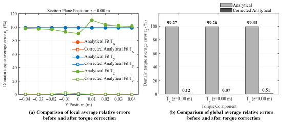
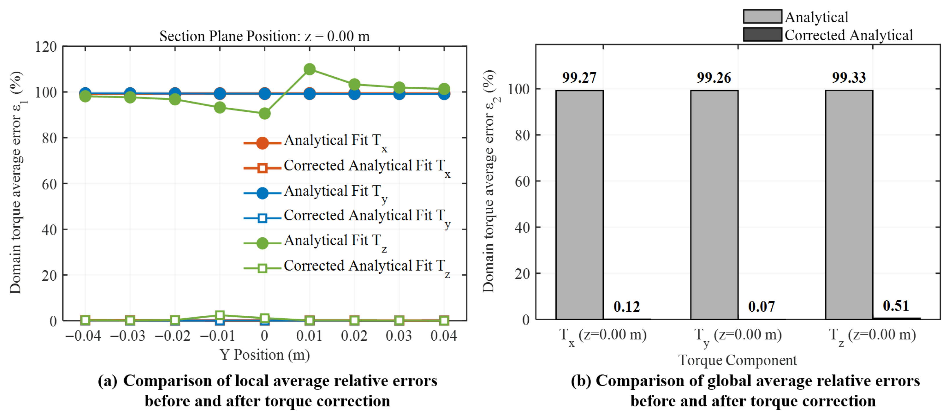
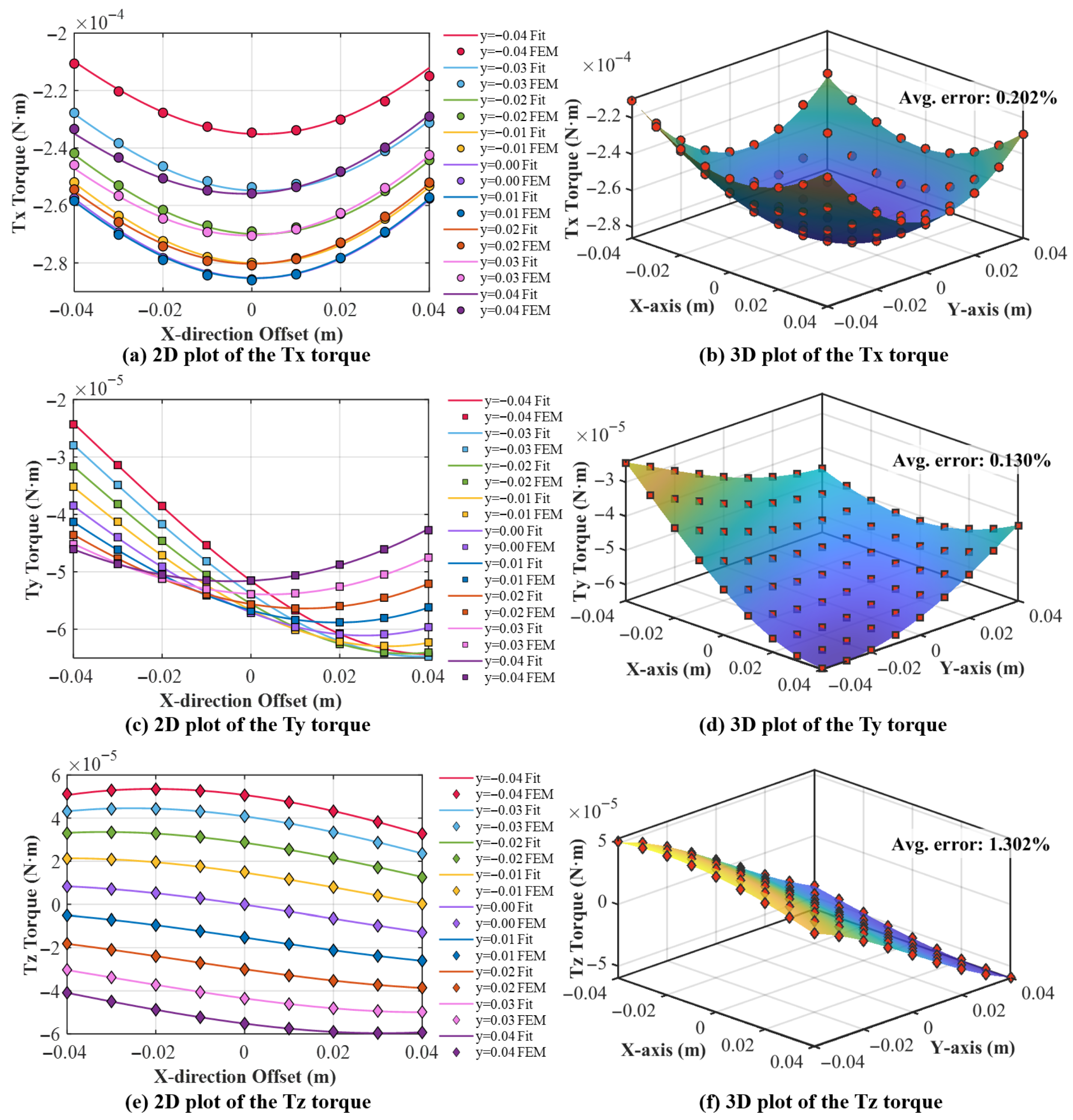
The comparison between the corrected approximate analytical results obtained by Equations (22)–(24) and the numerical results is shown in Figure 10, while the corresponding local and global average relative errors of both the uncorrected analytical model given by Equations (19)–(21) and the corrected analytical model given by Equations (22)–(24) are summarized in Figure 11. Figure 10a,c,e display the two-dimensional functional plots of Equations (22), (23), and (24), respectively, whereas Figure 10b,d,f show their corresponding three-dimensional fitted surfaces. All three corrected analytical expressions preserve the main distribution characteristics of the numerical results, including the overall variation trends and the rates of change along the x- and y-directions, and they agree well with the torque distributions previously observed in Figure 5, Figure 6 and Figure 7. Specifically, within the $xy$ plane at $z=0.00\mathrm{m}$, the corrected approximate analytical solutions derived from Equations (22)–(24) demonstrate strong agreement with the numerical data at the corresponding positions.

Figure 10. Comparison of finite-element and corrected approximate analytical solutions for the three electromagnetic torque components acting on the spherical shell in the plane $z=0.00\mathrm{m}$.

Figure 11. Comparison of local and global average relative errors of the analytical and corrected analytical torque models in the plane $z=0.00\mathrm{m}$.

As shown in Figure 11a, for the $T_x$ component, the local average relative error ${\epsilon }_1$ of the uncorrected analytical model ranges from $99.2161\%$ to $99.29\%$, whereas after correction it is reduced to 0.0760%∼0.2159%. The corresponding global average relative error ${\epsilon }_2$ shown in Figure 11b decreases from $99.2687\%$ to $0.1241\%$, indicating that the average accuracy of the corrected $T_x$ component is improved by $99.87\%$ compared with the uncorrected result. For the $T_y$ component, the local average relative error ${\epsilon }_1$ is reduced from 99.1352%∼99.41% to 0.0483%∼0.1045%, and the global average relative error ${\epsilon }_2$ decreases from $99.2598\%$ to $0.0677\%$. Therefore, the average accuracy of the corrected $T_y$ component is improved by $99.93\%$. Similarly, for the $T_z$ component, the local average relative error ${\epsilon }_1$ of the uncorrected analytical model ranges from $90.6156\%$ to $109.9598\%$, while after correction it decreases to 0.0445%∼2.4086%, as shown in Figure 11a. The corresponding global average relative error ${\epsilon }_2$ shown in Figure 11b decreases from $99.3278\%$ to $0.5138\%$. Thus, the average accuracy of the corrected $T_z$ component is improved by $99.48\%$ relative to the uncorrected result. These results indicate that the corrected approximate analytical expressions achieve sufficient computational accuracy and can therefore provide reliable theoretical support for subsequent dynamic modeling, real-time control, and rapid torque prediction.

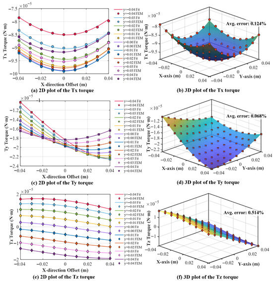
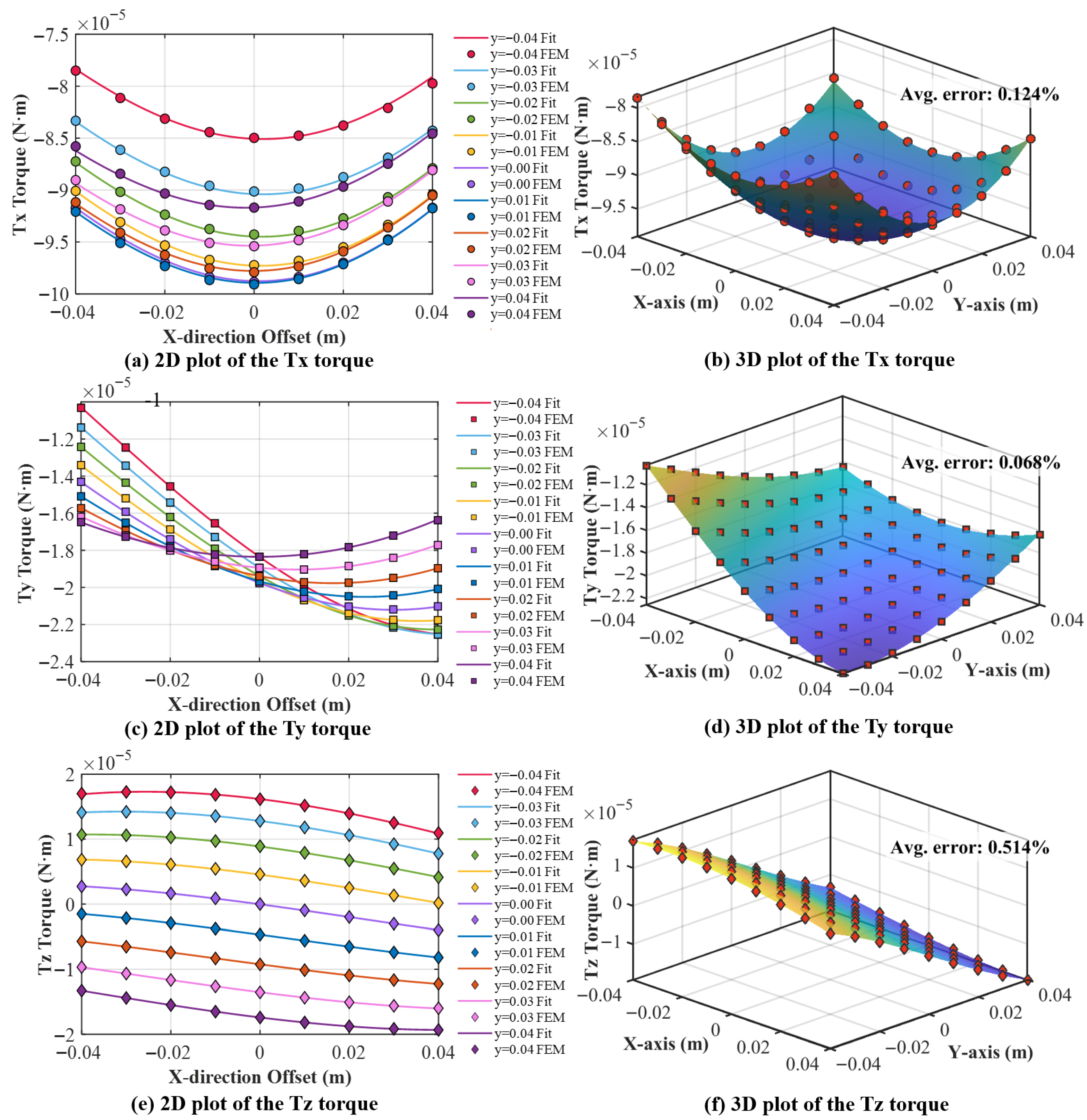
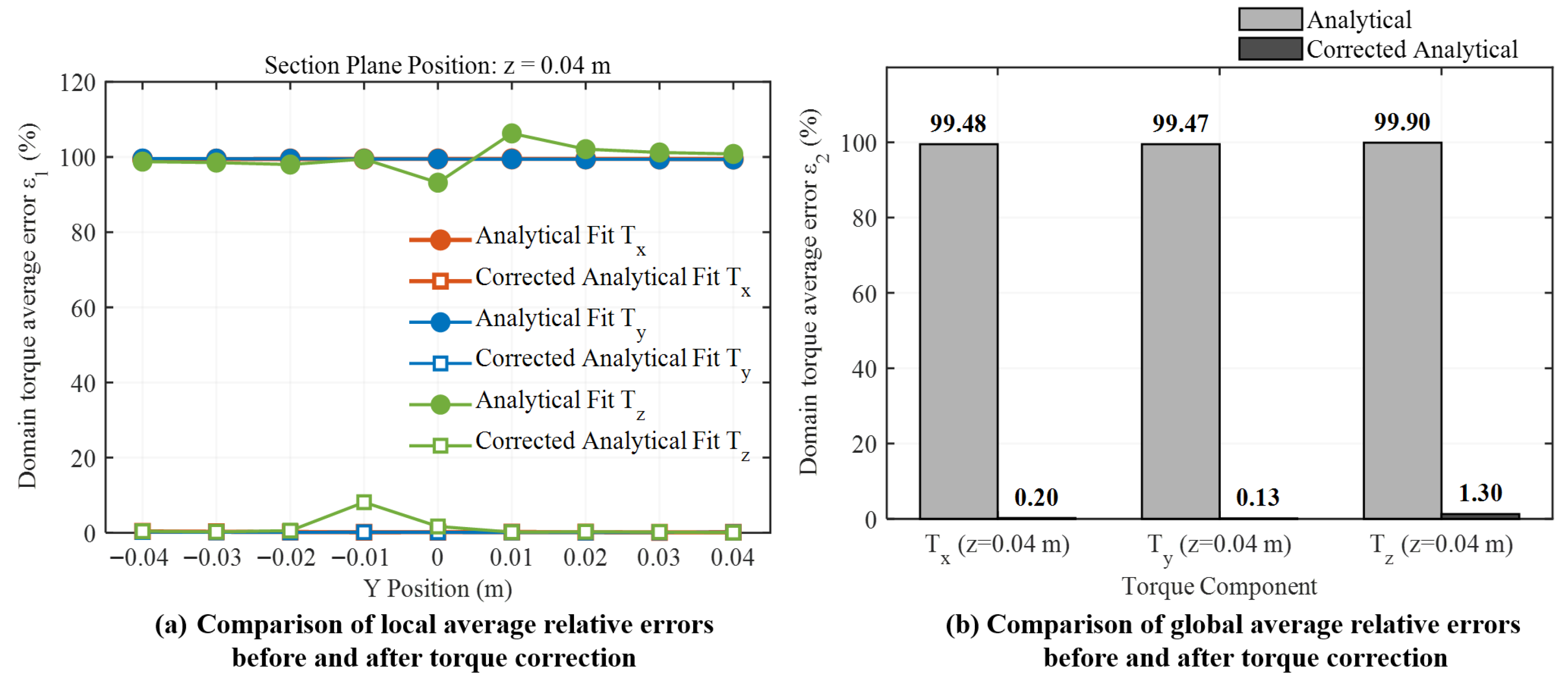
Figure 12 further verifies the fitting performance of Equations (22)–(24) on the plane $z=0.04\mathrm{m}$, and the corresponding local and global average relative errors are summarized in Figure 13. As shown in Figure 12, the corrected analytical curves and surfaces remain in close agreement with the numerical results for all three torque components, indicating that the corrected model still captures the main distribution characteristics and spatial variation trends on this section plane.

Figure 12. Comparison of finite-element and corrected approximate analytical solutions for the three electromagnetic torque components acting on the spherical shell in the plane $z=0.04\mathrm{m}$.

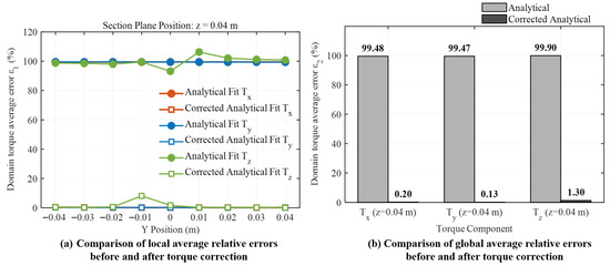
Figure 13. Comparison of local and global average relative errors of the analytical and corrected analytical torque models in the plane $z=0.04\mathrm{m}$.

As shown in Figure 13, after correction, the fitting accuracy of all three torque components on the plane $z=0.04\mathrm{m}$ is significantly improved. For $T_x$, the local average relative error ${\epsilon }_1$ is reduced from 99.4312%∼99.4982% to 0.1169%∼0.3717%, and the global average relative error ${\epsilon }_2$ decreases from $99.4784\%$ to $0.2020\%$, corresponding to an average accuracy improvement of $99.80\%$. For $T_y$, ${\epsilon }_1$ is reduced from 99.3706%∼99.5947% to 0.0857%∼0.2152%, while ${\epsilon }_2$ decreases from $99.4708\%$ to $0.1303\%$, giving an average accuracy improvement of $99.87\%$.

For $T_z$, the local average relative error ${\epsilon }_1$ decreases from 93.1767%∼106.2846% to 0.0693%∼8.1274%, and the global average relative error ${\epsilon }_2$ decreases from $99.8989\%$ to $1.3021\%$, corresponding to an average accuracy improvement of $98.70\%$. Therefore, the corrected approximate analytical expressions achieve sufficient computational accuracy and can provide reliable theoretical support for subsequent dynamic modeling, real-time control, and rapid torque prediction.

5.5. Electromagnetic De-Tumbling Simulation Under Nutational Motion

The angular-velocity attenuation of the nutating conducting spherical shell in the magnetic dipole field is further investigated based on the corrected electromagnetic torque model. The electromagnetic de-tumbling system is assumed to be composed of rigid bodies, and the magnetic source mounted at the end-effector of the servicing manipulator is assumed to maintain a fixed relative position with respect to the spherical shell during the considered de-tumbling interval. The center of the spherical shell is placed at $O_t=(0.01,0.01,0)\mathrm{m}$, which represents a typical bounded-offset configuration within the calibrated spatial domain. the rotational dynamics of the shell can be written as:

$${\mathbf{I}}_s\dot{\mathit{\omega }}+\mathit{\omega }\times \left({\mathbf{I}}_s\mathit{\omega }\right)={\mathbf{T}}_{\mathrm{s}}^{\mathrm{c}}$$

(27)

where ${\mathbf{I}}_s=\mathrm{diag}(I_x,I_y,I_z)$ is the inertia matrix of the spherical shell.

At each integration step, the instantaneous corrected electromagnetic torque is calculated from the current angular velocity and the prescribed bounded-offset position. The angular velocity is then updated by solving the rotational dynamic equation. The simulation parameters are listed in Table 3.

Table 3. Parameters used in the de-tumbling dynamic simulation.

Parameter	Value
Magnetic Dipole Moment (m)	$\mathrm{15,000}\mathrm{A}·{\mathrm{m}}^2$
Dipole-to-shell Distance (h)	$0.3\mathrm{m}$
Electrical Conductivity ($\sigma$)	$3.7\times {10}^7\mathrm{S}/\mathrm{m}$
Vacuum Permeability (${\mu }_0$)	$4\pi \times {10}^{-7}\mathrm{T}·\mathrm{m}/\mathrm{A}$
Shell Thickness (e)	$0.004\mathrm{m}$
Shell Radius (R)	$0.1\mathrm{m}$
Initial Angular Velocity ($\omega$)	${[8,1.6,1.6]}^{\mathrm{T}}\mathrm{deg}/\mathrm{s}$
Inertia Matrix (${\mathbf{I}}_s$)	$\mathrm{diag}(1600,1000,700)\mathrm{kg}·{\mathrm{m}}^2$
Simulation Time	10,000 s

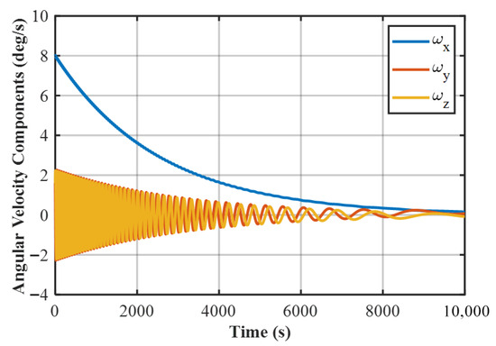
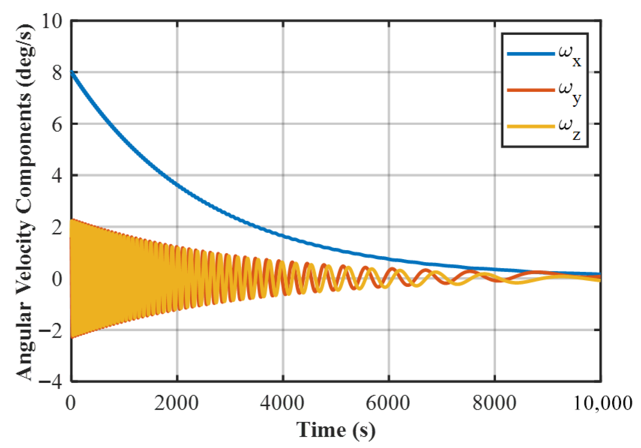
Figure 14 shows the time histories of the angular-velocity components. The initial angular velocity is dominated by the x-component, while the y- and z-components are smaller and exhibit coupled oscillatory variations during the de-tumbling process. Under the action of the corrected electromagnetic torque, ${\omega }_x$ decreases continuously, and the oscillation amplitudes of ${\omega }_y$ and ${\omega }_z$ also decay gradually. The three angular-velocity components tend toward zero as time increases, indicating that the electromagnetic torque produces a damping effect on the nutational motion.

Figure 14. Time histories of the angular-velocity components of the nutating conducting spherical shell.

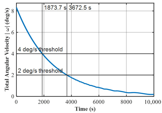
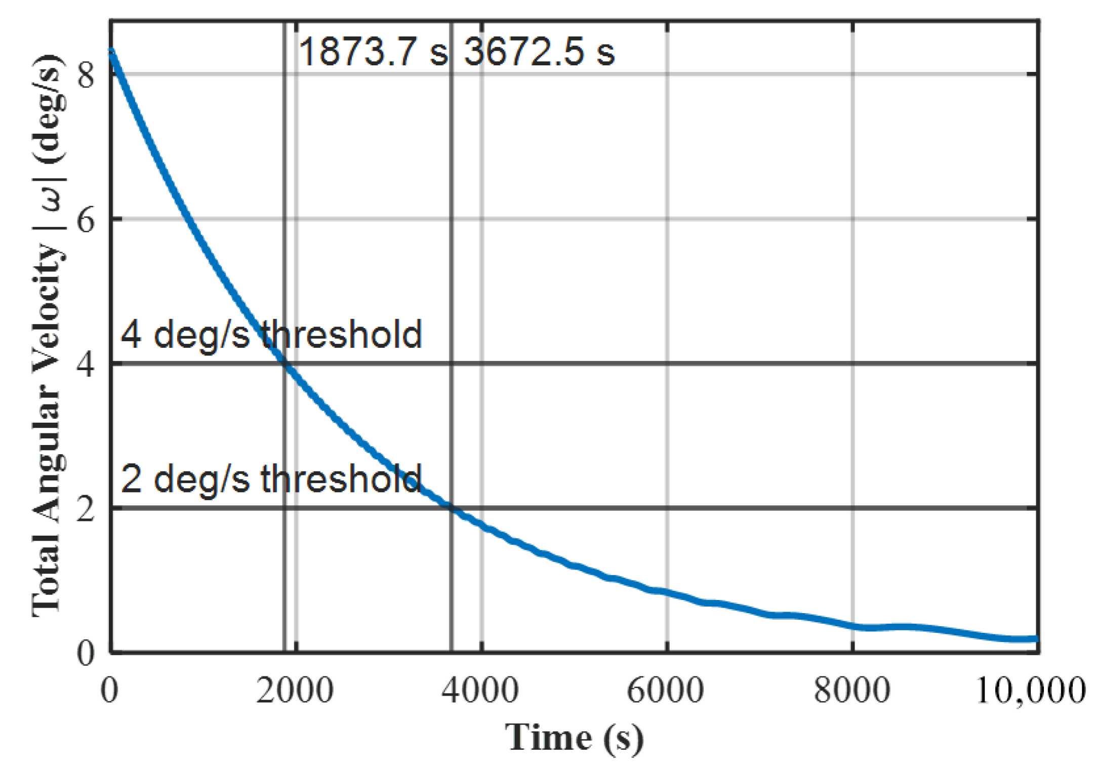
Figure 15 presents the time history of the total angular velocity, $\left|\mathit{\omega }\right|=\sqrt{{\omega }_x^2+{\omega }_y^2+{\omega }_z^2}$. The total angular velocity decreases from the initial value of approximately $8.31\mathrm{deg}/\mathrm{s}$ under the action of the corrected electromagnetic torque. It falls below $4\mathrm{deg}/\mathrm{s}$ at $t=1873.7\mathrm{s}$ [41], indicating that the rotational speed has entered the allowable range for robotic-arm capture. As the de-tumbling process continues, the total angular velocity further decreases below $2\mathrm{deg}/\mathrm{s}$ at $t=3672.5\mathrm{s}$, which provides a safer capture condition and further reduces the requirement on the capture control system. The decreasing trend of the angular velocity is consistent with the torque characteristics described by Equations (22)–(24), since the electromagnetic torque decreases with the reduction of the angular velocity. Therefore, the proposed corrected torque model provides a basis for evaluating the time-domain de-tumbling process of the nutating spherical shell under bounded positional offsets.

Figure 15. Time history of the total angular velocity and threshold-crossing times.

6. Conclusions

This paper investigated the electromagnetic torque acting on a nutating conducting spherical shell in a magnetic dipole field under bounded positional offsets. A mathematical model describing the relative position and electromagnetic interaction between the spherical shell and the fixed magnetic dipole was first established. On this basis, a finite-element simulation framework was constructed to calculate the spatial distributions of the three torque components within the bounded offset domain. The numerical results show that the electromagnetic torque under nutational motion contains three non-negligible components, namely, $T_x$, $T_y$, and $T_z$. Among them, $T_x$ is the dominant component, while $T_y$ and $T_z$ are secondary components. However, since all three components remain at comparable orders of magnitude, they should all be taken into account in subsequent modeling and correction. Based on the shell-center field approximation, approximate analytical expressions for the three electromagnetic torque components were derived. To compensate for the systematic deviation between the approximate analytical model and the finite-element results, polynomial correction terms were further introduced. The fitted results show that the correction of $T_x$ is mainly governed by low-order terms, whereas the corrections of $T_y$ and especially $T_z$ are more sensitive to higher-order spatial coupling. Nevertheless, the overall magnitudes of the fitted coefficients remain limited, which indicates that the original theoretical expressions preserve the correct physical structure, while the correction terms mainly provide compensation for residual local deviations. The corrected analytical model was validated on typical section planes, including $z=0.00\mathrm{m}$ and $z=0.04\mathrm{m}$. On the plane $z=0.00\mathrm{m}$, the global average relative errors of the corrected model are reduced to $0.1241\%$, $0.0677\%$, and $0.5138\%$ for $T_x$, $T_y$, and $T_z$, respectively. On the plane $z=0.04\mathrm{m}$, the corresponding errors are $0.2020\%$, $0.1303\%$, and $1.3021\%$. These results indicate that the corrected approximate analytical expressions attain sufficiently high computational accuracy and exhibit good consistency with the finite-element results over the bounded offset domain. Overall, the corrected approximate analytical model provides an effective basis for subsequent dynamic analysis, real-time control, and rapid electromagnetic torque prediction.

References

- Liou, J.C.; Johnson, N.L. Instability of the Present LEO Satellite Populations. Adv. Space Res. 2008, 41, 1046–1053. [Google Scholar] [CrossRef] [Scilit]
- ESA. ESA Space Environment Report 2025. Available online: https://www.esa.int (accessed on 31 March 2025).
- Liou, J. An Active Debris Removal Parametric Study for LEO Environment Remediation. Adv. Space Res. 2011, 47, 1865–1876. [Google Scholar] [CrossRef] [Scilit]
- Han, D.C.; Liu, Z.; Huang, P. Capture and Detumble of a Non-Cooperative Target without a Specific Gripping Point by a Dual-Arm Space Robot. Adv. Space Res. 2022, 69, 3770–3784. [Google Scholar] [CrossRef] [Scilit]
- Shan, M.; Guo, J.; Gill, E. Review and Comparison of Active Space Debris Capturing and Removal Methods. Prog. Aerosp. Sci. 2016, 80, 18–32. [Google Scholar] [CrossRef] [Scilit]
- Mankala, K.K.; Agrawal, S.K. Dynamic Modeling and Simulation of Impact in Tether Net/Gripper Systems. Multibody Syst. Dyn. 2004, 11, 235–250. [Google Scholar] [CrossRef] [Scilit]
- Reed, J.; Barraclough, S. Development of Harpoon System for Capturing Space Debris. In Proceedings of the 6th European Conference on Space Debris, Darmstadt, Germany, 22–25 April 2013. [Google Scholar]
- Huang, P.; Cai, J.; Meng, Z.; Hu, Z.; Wang, D. Novel Method of Monocular Real-Time Feature Point Tracking for Tethered Space Robots. J. Aerosp. Eng. 2013, 27, 04014039. [Google Scholar] [CrossRef] [Scilit]
- Yang, Z.; He, C.; Jing, Z.; Luo, J. DBN-TOPSIS-Based Multi-Space Non-Cooperative Target Threat Assessment Method. Aerosp. Shanghai 2025, 42, 158–170. [Google Scholar]
- Biesbroek, R.; Soares, T.; Husing, J.; Innocenti, L. The e.Deorbit CDF Study: A Design Study for the Safe Removal of a Large Space Debris. In Proceedings of the 6th European Conference on Space Debris, Darmstadt, Germany, 22–25 April 2013. [Google Scholar]
- Du, L.; Chen, Z.; Hu, H.; Liu, X.; Guo, Y. Design of De-Tumbling Device for Improving the De-Tumbling Performance of Uncooperative Space Target. Space Sci. Technol. 2024, 4, 0186. [Google Scholar] [CrossRef] [Scilit]
- Yu, Y.; Yue, H.; Zhao, H.; Yang, F.; Chen, X. Optimal Configuration of Distributed HTS Coils for the Non-Contact De-Tumbling of Space Debris. Acta Astronaut. 2022, 191, 491–501. [Google Scholar] [CrossRef] [Scilit]
- Hao, C.; Dai, H.; Yue, X. Optimal Nutation Suppressing Method for Detumbling Satellites via a Flexible Deceleration Device. Nonlinear Dyn. 2023, 111, 14977–14989. [Google Scholar] [CrossRef] [Scilit]
- Liu, Y.; Liu, X.; Cai, G.; Xu, F.; Tang, S. Detumbling a Non-Cooperative Tumbling Target Using a Low-Thrust Device. AIAA J. 2022, 60, 2718–2729. [Google Scholar] [CrossRef] [Scilit]
- Che, D.; Zheng, Z.; Yuan, J. An Innovate Detumbling Method for a Non-Cooperative Space Target via Repeated Tentative Contacts. IEEE Access 2022, 10, 64435–64450. [Google Scholar] [CrossRef] [Scilit]
- Ma, Z.; Liu, Z.; Zou, H.; Liu, J. Dynamic Modeling and Analysis of Satellite Detumbling Using a Brush Type Contactor Based on Flexible Multibody Dynamics. Mech. Mach. Theory 2022, 170, 104675. [Google Scholar] [CrossRef] [Scilit]
- Li, C.; Zheng, Z.; Yuan, J. Trajectory Tracking for Repeated-Impact-Based Detumbling Using a Multi-Arm Space Robot. Aerosp. Sci. Technol. 2023, 133, 108144. [Google Scholar] [CrossRef] [Scilit]
- Golebiowski, W.; Michalczyk, R.; Dyrek, M.; Battista, U.; Wormnes, K. Validated Simulator for Space Debris Removal with Nets and Other Flexible Tethers Applications. Acta Astronaut. 2016, 129, 229–240. [Google Scholar] [CrossRef] [Scilit]
- Zhang, Z.; Yu, Z.; Zhang, Q.; Zeng, M.; Li, S. Dynamics and Control of a Tethered Space-Tug System Using Takagi–Sugeno Fuzzy Methods. Aerosp. Sci. Technol. 2019, 87, 289–299. [Google Scholar] [CrossRef] [Scilit]
- Tiwari, A.S.; Nair, S.; Goldstein, D.B. Single- and Multinozzle Plume Impingement to Detumble Space Debris. J. Spacecr. Rockets 2024, 62, 945–954. [Google Scholar] [CrossRef] [Scilit]
- Kumar, R.; Sedwick, R.J. Despinning Orbital Debris Before Docking Using Laser Ablation. J. Spacecr. Rockets 2015, 52, 1–6. [Google Scholar] [CrossRef] [Scilit]
- Bennett, T.; Schaub, H. Touchless Electrostatic Three-Dimensional Detumbling of Large Axi-Symmetric Debris. J. Astronaut. Sci. 2015, 152, 233–253. [Google Scholar] [CrossRef] [Scilit]
- Gomez, N.O.; Walker, S.J.I. Eddy Currents Applied to De-Tumbling of Space Debris: Analysis and Validation of Approximate Proposed Methods. Acta Astronaut. 2015, 114, 34–53. [Google Scholar] [CrossRef] [Scilit]
- Yu, Y.; Yue, H.; Yang, F.; Zhao, H.; Lu, Y. Electromagnetic Interaction Between a Slowly Rotating Conducting Shell and Magnetic Dipoles: A Theoretical and Numerical Study. IEEE Trans. Magn. 2021, 57, 6302311. [Google Scholar] [CrossRef] [Scilit]
- Sugai, F.; Abiko, S.; Tsujita, T.; Jiang, X.; Uchiyama, M. Development of an Eddy Current Brake System for Detumbling Malfunctioning Satellites. In Proceedings of the IEEE/SICE International Symposium on System Integration, Nagoya, Japan, 11–13 December 2015. [Google Scholar]
- Du, L.; Chen, Z.; Hu, H.; Zhao, J.; Liu, X.; Zhang, Q.; Zhang, K. Contactless De-Tumbling of the Uncooperative Targets Using Arc-Linear Electromagnetic Device. Adv. Space Res. 2022, 71, 3290–3300. [Google Scholar] [CrossRef] [Scilit]
- Du, L.; Chen, Z.; Hu, H.; Liu, X.; Guo, Y. An Improved Uncooperative Space Target De-Tumbling Method Using Electromagnetic De-Tumbling Devices with AC Excitation. Adv. Space Res. 2025, 75, 1264–1276. [Google Scholar] [CrossRef] [Scilit]
- Walker, S.J.I.; Gomez, N.O. Guidance, Navigation, and Control for the Eddy Brake Method. J. Guid. Control Dyn. 2017, 40, 52–68. [Google Scholar]
- Liu, X.; Lu, Y.; Zhang, Q.; Zhang, K. An Application of Eddy Current Effect on the Active Detumble of Uncontrolled Satellite with Tilt Air Gap. IEEE Trans. Magn. 2019, 55, 1–11. [Google Scholar] [CrossRef] [Scilit]
- Meng, Q.; Zhao, C.; Ji, H.; Liang, J. Identify the Full Inertial Parameters of a Non-Cooperative Target with Eddy Current Detumbling. Adv. Space Res. 2020, 66, 7. [Google Scholar] [CrossRef] [Scilit]
- Pham, L.N.; Tabor, G.F.; Pourkand, A.; Aman, J.L.B.; Hermans, T.; Abbott, J.J. Dexterous Magnetic Manipulation of Conductive Non-Magnetic Objects. Nature 2021, 598, 439–443. [Google Scholar] [CrossRef] [Scilit]
- Allen, T.J.; Sperry, A.J.; Posselli, N.R.; Minor, B.A.; Abbott, J.J. Characterization of a Rotating Magnetic Dipole Field for Contactless Detumbling of Space Debris. In Proceedings of the 2024 International Conference on Space Robotics (iSpaRo); IEEE: Piscataway, NJ, USA, 2024; pp. 119–124. [Google Scholar]
- Barker, L.M.; Allen, T.J.; Sperry, A.J.; Abbott, J.J. Revisiting the Far-Field Model of the Force and Torque Induced on a Conductive Nonmagnetic Sphere by a Rotating Magnetic Dipole. Sci. Rep. 2025, 15, 18194. [Google Scholar] [CrossRef] [Scilit]
- Khan, S.A.; Yang, S.; Ali, A.; Tahir, M.; Fahad, S.; Rao, S.; Waseem, M. PCB-integrated embedded planar magnetorquers for small satellites intelligent detumbling. Comput. Electr. Eng. 2023, 108, 108719. [Google Scholar] [CrossRef] [Scilit]
- Smith, G.L. A Theoretical Study of the Torques Induced by a Magnetic Field on Rotating Cylinders and Spinning Thin-Wall Cones, Cone Frustums, and General Body of Revolution; NASA: Washington, DC, USA, 1962. [Google Scholar]
- Ormsby, J.F. Eddy Current Torques and Motion Decay on Rotating Shells. In Eddy Current Torques and Motion Decay on Rotating Shells; The MITRE Corporation: Bedford, MA, USA, 1967. [Google Scholar]
- Youngquist, R.C.; Nurge, M.A.; Starr, S.O.; Leve, F.A.; Peck, M. A Slowly Rotating Hollow Sphere in a Magnetic Field: First Steps to De-Spin a Space Object. Am. J. Phys. 2016, 84, 181–191. [Google Scholar] [CrossRef] [Scilit]
- Nurge, M.A.; Youngquist, R.C.; Caracciolo, R.A.; Peck, M.; Leve, F.A. A Thick-Walled Sphere Rotating in a Uniform Magnetic Field: The Next Step to De-Spin a Space Object. Am. J. Phys. 2017, 85, 596–610. [Google Scholar] [CrossRef] [Scilit]
- Yu, Y.; Yang, F.; Yue, H.; Lu, Y.; Zhao, H. Prospects of De-Tumbling Large Space Debris Using a Two-Satellite Electromagnetic Formation. Adv. Space Res. 2021, 67, 1816–1829. [Google Scholar] [CrossRef] [Scilit]
- Jackson, J.D. Classical Electrodynamics; Wiley: Hoboken, NJ, USA, 2007. [Google Scholar]
- Castronuovo, M.M. Active Space Debris Removal—A Preliminary Mission Analysis and Design. Acta Astronaut. 2011, 69, 848–859. [Google Scholar] [CrossRef] [Scilit]
Disclaimer/Publisher’s Note: The statements, opinions and data contained in all publications are solely those of the individual author(s) and contributor(s) and not of MDPI and/or the editor(s). MDPI and/or the editor(s) disclaim responsibility for any injury to people or property resulting from any ideas, methods, instructions or products referred to in the content. |
© 2026 by the authors. Licensee MDPI, Basel, Switzerland. This article is an open access article distributed under the terms and conditions of the Creative Commons Attribution (CC BY) license.