Decoupling Global and Local Faults in Satellite Swarms Using Smart-Freeze Adaptation and Isolation-Priority Logic

Abstract

Satellite swarm operations require robust methodologies to distinguish between leader-induced reference frame biases (global errors) and individual follower anomalies (local deviations). This is the challenge of distributed fault diagnosis. In leader–follower topologies, distinguishing between a global reference error (leader satellite broadcasting incorrect navigation data) and a local node error (follower satellite drifting) is mathematically ambiguous when we use standard methods. Even recent unsupervised frameworks, such as Model-Guided Online Transfer Learning (MGOTL), that excel at single-satellite component diagnosis, suffer from adaptation and signal bleed when they are applied directly to distributed topologies. Therefore, we propose the Isolation-First Consensus Anomaly Detection (IF-CAD) framework for Decoupling Global and Local Faults in Satellite Swarms. We introduce a Smart Freeze mechanism to prevent the learning of persistent faults and a hierarchical logic that prioritizes local isolation over global agreement. The IF-CAD framework successfully decouples global leader faults from local follower faults. Fault detection remains stable even during long-duration anomalies.

1. Introduction

In leader–follower satellite swarms, the diagnostic process is frequently complicated by the overlap between different failure scales. The challenge lies in distinguishing global reference biases, where the leader propagates incorrect navigation data, from local node faults, where an individual follower’s actuator or sensor fails. Rapidly isolating these two error types prevents the swarm from incorrectly adapting to a corrupted reference, a scenario that leads to catastrophic model divergence and mission failure [1]. In a leader–follower topology, the leader satellite defines the local reference frame. Therefore, a fault in the leader’s navigation system is a global error vector across the entire swarm, while a fault in a follower is a local deviation vector.

Fault Detection and Isolation (FDI) for spacecraft usually relies on model-based methods, such as Kalman Filters (Ghasemi and Khorasani 2015 [2], Chen et al., 2024 [3], Jiao et al., 2024 [4], Mounier et al., 2025 [5], Li et al., 2025 [6], and Patan et al., 2026 [7]) and parity space approaches (Kim et al., 2005 [8], Ashtiani 2007 [9], Odendaal et al., 2014 [10], Hegenbald 2014 [11], and Zhong et al., 2018 [12]). These methods are effective for known failure modes, but they do not distinguish between global and local failures. They also struggle with the non-linear environmental disturbances in Low Earth Orbit (LEO). To address these limitations, data-driven approaches have gained attention. Methods using Deep Autoencoders (Xiang 2020 [13]) and Long Short-Term Memory (LSTM) networks (Dhanagopal 2020 [14]) have shown success in detecting anomalies in high-dimensional telemetry data without explicit physical modeling.

We must also note that effective swarm coordination relies on robust information distribution, whether through GNSS-based navigation tasks [15], angles-only navigation for deep space [16], or optimized communication architectures [17]. While these works optimize how data is shared, they assume the shared data is truthful. In broader multi-agent systems, this challenge is framed as a consensus problem, where global agreement emerges from local interactions [18]. These distributed algorithms can reach consensus on various general functions, with average consensus being a common special case, though their security remains a critical concern regarding channel tampering or edge faults [19,20]. Our work builds upon these architectures by adding a decentralized verification layer to detect and isolate erroneous data before it is integrated into the swarm’s collective state.

Coordinated swarm behavior requires not only robust control laws but also sophisticated scheduling. Recent work in space situational awareness has highlighted the importance of multi-objective early warning mission planning by using algorithms like NSGA-II to aggregate critical tasks across multiple satellites [21]. While such planning optimizes mission efficiency, the underlying assumption is that all nodes remain fault-free, a gap that our proposed framework aims to bridge.

In addition to mission planning, the resilience of cooperative swarms is often tested during the recovery of failed assets. For instance, recent research has explored RBF Neural Network-based cooperative electromagnetic takeover control for large-scale failed spacecraft [22]. This approach demonstrates the potential for active recovery through cooperative control laws. However, for such takeover mechanisms to be effectively deployed, the swarm must first accurately isolate the source of the failure. The framework presented here provides this critical diagnostic foundation.

Plus, high-fidelity maneuvers in non-circular or eccentric orbits require precise state transition models, such as the analytical sensitivity matrices developed for near-optimal elliptical transfers [23]. These advancements significantly improve the accuracy of swarm reconfigurations. However, their performance is tied to the integrity of the navigation data. Our proposed framework builds upon these high-precision dynamics by providing a decentralized diagnostic layer that guarantees that the Smart-Freeze logic protects the swarm’s state estimation from propagated reference errors.

Similarly, high-precision control strategies are essential for specialized missions; for instance, Power Rate Reaching Law Sliding Mode Control (PRRL-SMC) has recently been proposed to enhance robustness during CubeSat debris capture maneuvers [24]. While these advancements improve the execution of satellite missions, they typically assume a healthy operational baseline. This shows the need for the diagnostic resilience that is provided by our proposed framework.

Our work is inspired by the Model-Guided Online Transfer Learning (MGOTL) framework proposed by Xia & Meng 2025 [25]. They successfully introduce a physics-guided residual generator combined with continuous online learning to detect faults in internal components (e.g., reaction wheels). While [25] shows high efficacy for single-satellite subsystems, an evolution of the method is necessary so that it can also be applied to satellite swarms without stability issues.

In formation flying, relative states are coupled. A fault in one node changes the residuals of others. Such Online Transfer Learning (OTL) frameworks often do not distinguish the source of the error in such a coupled topology. This results in signal bleed, where a local fault is misdiagnosed as a system-wide failure. That is why we propose a method inspired by [25] that is effective in swarm topologies.

The motivation for this work is that swarm stability is compromised during persistent reference-frame biases, hereafter referred to as Global Reference Anomalies. The Global Reference Anomalies scenario refers to when a leader satellite develops a persistent bias, and the follower satellites that operate on standard consensus logic mistakenly conclude that they are all out of position. This is due to the inherent trust and dependence of follower navigation systems on the state-vector broadcasts provided by the leader node. Plus, standard online learning algorithms tend to adapt to persistent faults. So, they learn that the false state is the new normal.

The objective of this study is to develop a distributed fault attribution framework that addresses the challenge of model adaptation while robustly distinguishing between global reference frame shifts and local actuation failures. To achieve this, a hierarchical diagnostic logic is proposed: rather than performing simple binary anomaly detection, the system evaluates the statistical uniqueness of node-specific deviations through a comparative isolation protocol. In this architecture, an anomaly characterized by a solitary node divergence is attributed to a local agent failure. Conversely, synchronous residuals across the collective swarm topology are classified as a global reference error originating from the leader node. Furthermore, to prevent fault assimilation, where the adaptive model mistakenly learns to accept anomalous data as a healthy baseline, the adaptation mechanism is programmatically suspended upon the detection of a statistical outlier. This ‘Smart-Freeze’ protocol ensures the integrity of the nominal state distribution and prevents model convergence toward a degraded or anomalous steady state. In technical terms, this paper extends the foundational concepts of MGOTL [25] into the distributed domain.

The fundamental problem addressed in this study is the diagnostic ambiguity inherent in leader–follower satellite swarms. Formally, given a swarm of $N$ agents, the goal is to distinguish between a global state deviation $\mathsf{\Delta }{X}_g$ (originated from a leader’s reference bias) and a local node fault $f_i$ (originated from a specific follower’s actuator/sensor). The goal is to design a decentralized logic that satisfies two criteria:

• Isolation Accuracy: The probability of misclassifying a leader drift as a local fault must be minimized to prevent incorrect model updates.
• Model Integrity: The adaptive learning parameters must remain stable (convergent) even during persistent anomalies, a requirement addressed by the Smart-Freeze protocol and the Lyapunov-based stability analysis.

The main contributions of this work are summarized as follows:

• Decoupling of Hierarchical Faults: We propose a novel Isolation-Priority logic that uses topological residuals to differentiate between global reference frame biases and local node failures. This guarantees that a leader’s drift is not incorrectly assimilated as a local healthy state.
• Resilient Adaptation via Smart-Freeze: We introduce a conditional switching mechanism for Online Transfer Learning (OTL). By theoretically bounding the learning rate during anomalous transients, we preserve the healthy model baseline and prevent parameter divergence. This technique offers a significant improvement over traditional adaptive filters.

The remainder of this paper is organized as follows: Section 2 details the mathematical formulation of the IF-CAD framework; Section 3 presents the simulation results and performance analysis; and Section 4 provides the concluding remarks.

2. Modeling

2.1. System Dynamics

The relative accelerations ($\ddot{x},\ddot{y},\ddot{z}$) of a Follower are governed by the orbital mean motion $n=\sqrt{\mu /a^3}$, where $\mu$ is the standard gravitational parameter, and $a$ is the semi-major axis. The scalar differential equations are as follows [26].

$$\begin{array}{ll}\ddot{x}& =3n^{2}x+2n\dot{y}+u_x+d_x\\ \ddot{y}& =-2n\dot{x}+u_y+d_y\\ \ddot{z}& =-n^{2}z+u_z+d_z\end{array}$$

(1)

Here, $u$ represents the control thrust and $d$ represents environmental disturbances (such as $J_2$ perturbation, atmospheric drag, and so on). In our simulation, $n = 0.0011$ rad/s, which means the satellite completes a full 360-degree orbit ($2\pi$ radians) in about 5.712 s (roughly 95 min), which is typical for a Low Earth Orbit (LEO). $a$ is the distance from the center of the Earth to the satellite.

These equations show the counterintuitive coupling in orbital mechanics, which naive learning algorithms might mistake for sensor anomalies, as follows.

1

The Speed–Altitude Coupling ($2n\dot{y}$): As seen in Equation (1) ($\ddot{x}=3n^{2}x+2n\dot{y}+u_x+d_x$), increasing velocity in the along-track direction ($\dot{y}>0$) creates a Coriolis acceleration in the radial direction ($x$). This induces a radial displacement, which, in accordance with Keplerian dynamics, results in a reduction of the mean orbital velocity. Prograde acceleration results in an increase in the orbital semi-major axis, transitioning the craft into a higher-energy trajectory. At the higher point (apogee), your velocity is actually lower than it was at the original altitude.

2

The Drift Trap ($-2n\dot{x}$): As seen in Equation (1) ($\ddot{y}=-2n\dot{x}+u_y+d_y$), a radial drift ($\dot{x}>0$) induces a backward acceleration along the track. This coupling means a fault in the $x$-axis thruster will manifest as a trajectory error in the $y$-axis, and confuse standard diagonal-only fault detection logic. Radial thrusting generates a coupled along-track displacement; therefore, a primary fault in the radial actuator manifests as a dominant secular drift in the longitudinal axis.

For implementation in the IF-CAD framework, we write these equations into a continuous Linear Time Invariant (LTI) state-space model, $\dot{X}=AX+BU+D$, where the state vector is $X={\left[x,y,z,\dot{x},\dot{y},\dot{z}\right]}^T$. Matrix A tells us how X will change naturally if no thrusters are fired. Matrix B tells us how that state changes if thrusters (u) are fired. The matrices $A$ and B are as follows:

$$A=\left[\begin{array}{cccccc}0& 0& 0& 1& 0& 0\\ 0& 0& 0& 0& 1& 0\\ 0& 0& 0& 0& 0& 1\\ 3n^2& 0& 0& 0& 2n& 0\\ 0& 0& 0& -2n& 0& 0\\ 0& 0& -n^2& 0& 0& 0\end{array}\right] , \mathrm{B} = \left[\begin{array}{c}\begin{array}{c}0 0 0\\ 0 0 0\\ 0 0 0\\ 1 0 0\\ 0 1 0\end{array}\\ 0 0 1\end{array}\right]$$

(2)

We must also note that rows 1–3 of Matrix A represent the kinematic identity ($\dot{r}=v$), and rows 4–6 represent the orbital dynamics derived in Equation (1).

The residual $r\left(t\right)$ results in the following

$$r_i\left(t\right)=|P_{measured,i}-P_{target,i}|,$$

(3)

where $P_{target,i}$ is the expected value of state variable i, i.e., for the discrete case, replacing time t with step k, we can use $P_{target}\left(k\right)=\mathrm{A}\mathrm{X}\left(\mathrm{k}-1\right)+\mathrm{B}\mathrm{U}\left(\mathrm{k}-1\right)$.

This means the residual is the difference between the measured position and the target geometry. $P_{target,i}$ is the predicted state generated by the physics model, Equation (2). The residual r(t) is the prediction error. It is the difference between where the physics indicates the satellite should be and where the sensors observe it.

2.2. Applying MGOTL

Online Transfer Learning (OTL) is the adaptive brain that prevents the fault detector from being too sensitive. Without it, simple sensor noise or tiny orbital disturbances would result in a prohibitively high False Alarm Rate (FAR) and reduced diagnostic sensitivity. Some fault detectors might use a fixed threshold (If error > some number, then Fault). However, satellites change over time due to temperature or sensor aging. Instead of a fixed threshold, OTL constantly learns what normal looks like for a specific satellite at a specific time.

To validate our approach, we take the core principle of the MGOTL framework as described in [25] and apply it to satellite swarm dynamics. The MGOTL framework is designed to detect faults by comparing real-time telemetry with a physics-informed model. This process involves two mathematical steps: the Online Transfer Learning update and the Wasserstein Anomaly Scoring [25]. The framework employs an online model $M_{OTL}$ that adaptively learns the system’s current healthy state representation. For components with lower time-series complexity, such as the satellite actuators and orbit residuals, the system uses Bayesian Ridge Regression (BRR).

The online model is initialized with parameters from an offline source model $M_S$ and is updated recursively at each time step k based on the prediction error of the target domain data $X^T$. The update strategy follows a performance-based weighting that shifts reliance toward the model with the lowest prediction error as follows:

$$M_{OTL}^k=\mathrm{f}\left({\mathrm{M}}_s,{\mathrm{X}}_k^T\right).$$

(4)

This continuous update allows the model to adapt to environmental drift and sensor aging, but it creates a vulnerability: in the presence of a persistent step fault, the recursive update process eventually assimilates the anomalous signal into its new normal mean.

To determine if the system has deviated from its healthy baseline, the framework calculates an anomaly score using the p-order Wasserstein distance (${\mathrm{W}}_p$). This metric measures the statistical divergence between the distribution of the healthy initial state $M_{OTL}$ and the current online state $M_{OTL}^k$ [25].

$${{\mathrm{W}}_p(M}_{OTL}^0{,M}_{OTL}^k)={({\displaystyle \frac{1}{N_d}}\sum _{i=1}^{N_d}{|\left|M_{OTL}^0\left(i\right)-M_{OTL}^k\left(i\right)\right||}^p)}^{{\displaystyle \frac{1}{p}}}$$

(5)

where $M_{OTL}^0$ is the model evaluation matrix for the satellite’s normal state and $N_d$ is a normalization constant.

Faults are declared using an adaptive threshold detector. After each alarm or system reset, the system calculates the maximum and minimum Wasserstein distances within a time window [$t_a+N_a,t_a+N_a+N_t$] to set new upper and lower bounds. A fault is confirmed if the ratio of data points exceeding these thresholds ($N_s$) over a detection window ($N_{\omega }$) exceeds a tolerance $\epsilon$ as follows [25]. Please consider that $N_{\omega }$ is a specific time window or set of data points used to monitor system performance, and $N_s$ is the number of data points within that detection window ($N_{\omega }$) that exceed the calculated upper or lower bounds of the Wasserstein distance.

$${\displaystyle \frac{N_s}{N_{\omega }}}>\epsilon$$

(6)

2.3. The Proposed IF-CAD Framework

The Isolation-First Consensus Anomaly Detection (IF-CAD) improves on the MGOTL baseline by adding a conditional control layer to the learning process and a relational logic layer to the swarm topology.

2.3.1. The Smart Freeze Logic

Traditional Online Transfer Learning (OTL) suffers from fault absorption, where the recursive update mechanism eventually accepts a persistent anomaly as the new healthy baseline. IF-CAD resolves this by implementing a conditional update rule, governed by the current anomaly score $S_i\left(t\right)$. The statistical baseline ${\mu }_t$ is updated as follows:

$${\mu }_t=\left\{\begin{array}{ll}\left(1-\alpha \right){\mu }_{t-1}+\alpha \cdot r_t& \mathrm{if} S_i\left(t\right)<\tau \\ {\mu }_{t-1}& \mathrm{if} S_i\left(t\right)\ge \tau \end{array}\right. ,$$

(7)

where $r_t$ represents the model-guided residual derived from Equation (3), $\alpha$ is the learning rate (set to $0.05$ in simulation), and $\tau$ is the sensitivity threshold. By forcing the learning rate to zero when $S_i\left(t\right)\ge \tau$, the framework freezes and does not adapt to the fault.

2.3.2. Topological Metrics: Consensus and Isolation

In a leader–follower swarm, a fault in the leader’s state is perceived by all followers as a simultaneous deviation. To decouple these effects, IF-CAD defines two metrics calculated across the set of $L$ active communication links.

1

Global Consensus Score ($G$): This metric represents the collective deviation of the swarm relative to the leader. It is defined as the arithmetic mean of the Wasserstein anomaly scores across all links, and is a form of Average Consensus, a well-documented concept in swarm control, as follows [27].

$$G\left(t\right)={\displaystyle \frac{1}{L}}\sum _{i=1}^L{S}_i\left(t\right)$$

(8)

2

Isolation Ratio ($R_i$): To identify faults unique to a specific agent, the isolation ratio measures the dominance of a single link’s score relative to the swarm average. So we define $R_i$ as follows.

$$R_i\left(t\right)={\displaystyle \frac{S_i\left(t\right)}{G\left(t\right)+ϵ}}$$

(9)

where $ϵ$ is a small regularization constant ($1\times {10}^{-6}$) to ensure numerical stability. While consensus-based averaging (Equation (8)) is a standard approach in distributed sensing [27], the unique contribution of IF-CAD is the coupling of this metric with the Isolation-Priority logic defined in Equation (9).

2.3.3. Isolation-First Decision Logic

The framework utilizes a hierarchical decision gate to attribute faults. To minimize false global alarms, the logic prioritizes local isolation over global consensus. Based on the scores calculated in Equations (2) and (3), the decision is made as follows:

1

Local Follower Fault: If $R_i\left(t\right)>\Gamma$ and $S_i\left(t\right)>\tau$, the anomaly is classified as a local failure in Follower $i$.

2

Global Leader Fault: If the isolation criteria are not met ($R_i\left(t\right)\le \Gamma$) but $G\left(t\right)>\tau$, the anomaly is attributed to the Leader.

This isolation-priority approach prevents signal bleed, where a leader’s maneuver error might otherwise be misinterpreted as multiple simultaneous follower faults.

2.3.4. Parameter Tuning and Sensitivity

The performance of the IF-CAD framework is governed by the detection threshold ($\tau$) and the isolation threshold ($\mathsf{\Gamma }$). These are tuned based on the statistical properties of the nominal system:

1

Detection Threshold ($\tau$): This parameter is set relative to the sensor noise floor ($\sigma$). In this study, $\sigma =0.005$ m. Under nominal conditions, the Wasserstein distance residuals follow a Chi-squared-like distribution. To maintain an FAR below 0.1%, $\tau$ is set using a $k\sigma$ heuristic. For the simulated environment, $\tau =10$ represents the 99th percentile of the noise-induced residuals.

2

Isolation Threshold ($\mathsf{\Gamma }$): This represents the Topological Dominance Factor. To distinguish a local fault from a global bias, the anomaly score of a single link must significantly outweigh the swarm average. We define $\mathsf{\Gamma }$ as follows.

$$\mathsf{\Gamma }>{\displaystyle \frac{Local Fault Magnitude}{Average Collective Noise}}$$

(10)

3

Based on our sensitivity analysis, $\mathsf{\Gamma }=5$ was chosen as the optimal knee point, that makes sure that leader-side biases are not incorrectly isolated as local follower faults.

2.3.5. Theoretical Analysis and Stability

The theoretical stability of the IF-CAD framework is established by ensuring that the adaptive model parameters remain bounded, even in the presence of persistent faults. This is achieved by regulating the model’s learning state to prevent fault assimilation.

1

Convergence in Nominal Conditions: Under nominal operating conditions, the model parameters $\theta$ function as a recursive estimator. Given a small learning rate ($\alpha =0.05$) and bounded Gaussian sensor noise $ϵ\sim \mathcal{N}\left(0,{\sigma }^2\right)$, the parameter update law is governed by:

$${\theta }_{t+1}=\left(1-\alpha \right){\theta }_t+\alpha \varphi \left(x_t\right)$$

(11)

where $\varphi \left(x_t\right)$ represents the observed state features at time $t$. In this mode, the system is Input to State Stable (ISS). As long as the input noise is bounded, the estimation error remains bounded, and $\theta$ converges to the mean manifold of the healthy orbital dynamics.

2

Stability Lock via Smart-Freeze Logic: The primary risk in adaptive swarm architectures is the absorption of global biases into the local model. If a leader satellite exhibits a secular drift, a standard adaptive filter will eventually treat this drift as the new normal, which results in parameter divergence. To prevent this, IF-CAD implements a Conditional Switching Law for the learning rate $\alpha$:

$$\alpha =\left\{\begin{array}{ll}0.05,& \mathrm{if} W\le \tau (\mathrm{Nominal} \mathrm{Mode})\\ 0,& \mathrm{if} W>\tau (\mathrm{Anomaly} \mathrm{Mode})\end{array}\right.$$

(12)

When the Wasserstein distance $W$ exceeds the detection threshold $\tau$, the system triggers the Smart-Freeze protocol. By setting $\alpha =0$, the update law simplifies to the following.

$${\theta }_{t+1}={\theta }_t$$

(13)

This mathematical lock guarantees that the healthy baseline is preserved in the model’s memory. This guarantees that the residual $W$ remains large and persistent throughout the fault duration, providing a formal safeguard against model divergence.

3

Robustness of the Isolation Decision: The stability of the diagnostic decision (distinguishing Global vs. Local faults) is enforced by the Isolation Ratio Γ. By requiring that, the following holds.

$${\mathcal{R}}_i(\mathrm{t})={\displaystyle \frac{W_i}{\frac{1}{N}\sum _{j=1}^N{W}_j}}\ge \Gamma$$

(14)

the system establishes a statistical buffer zone. This prevents chattering (unstable, rapid switching between fault classifications) that might otherwise be triggered by transient communication drops or minor sensor glitches. This guarantees a consistent and reliable diagnostic output.

3. Results and Discussion

Our Isolation-First Consensus Anomaly Detection (IF-CAD) framework enhances the foundation of [15] by adding two protective layers: Isolation-Priority logic and a Smart-Freeze mechanism. These components function as a hierarchical validation layer. They temporarily pause the learning process if the swarm cannot reach a consensus on the source of the error. By freezing the models during these global deviations, the system remains stable and accurate even in complex, multi-satellite formations.

3.1. Simulation

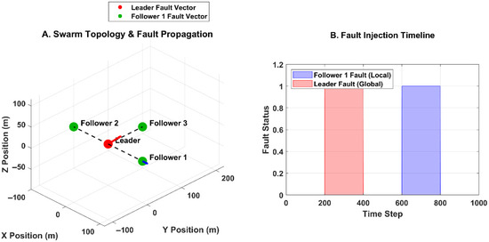
We simulated a 4-satellite swarm in Earth LEO ($h=500\mathrm{km}$) maintaining a tetrahedron formation with 100 m separation. The simulation includes full orbital propagation and Gaussian sensor noise (${\sigma }_{noise}\approx 5\mathrm{cm}$). Two distinct fault scenarios were injected as follows.

1.

Global Reference Fault (Leader): A sudden GPS broadcast bias of 15 m is injected into the Leader at $t\in \left[\mathrm{200,400}\right]$

2.

Local Component Fault (Follower 1): A physical position bias of 12 m is injected into Follower 1 at $t\in \left[600,800\right]$

Figure 1, part A, shows the Swarm Topology and Fault Propagation. It is a satellite swarm architecture that consists of one leader satellite and three follower satellites arranged in a tetrahedral formation. We have shown the inter-satellite communication links by black dashed lines. All followers communicate directly with the leader. This figure also shows two fault vectors regarding two distinct fault scenarios. It shows the Leader Fault Vector, which is a 20-m bias in all three coordinate directions (X, Y, Z), and is a global reference fault that affects all follower measurements simultaneously. It also shows Follower 1 Fault Vector, which is a 15-m bias exclusively in the X-direction, that is a local component fault that only affects measurements from Follower 1.

Figure 1. Swarm architecture and fault injection timeline.

Figure 1A is the topology that demonstrates the fundamental challenge in distributed fault detection, with the blue color showing the trajectory direction. We want to distinguish which fault comes from the leader and which comes from the followers.

Figure 1B shows the Fault Injection Timeline. It is the precise timing and duration of fault injections during the 1000-step simulation. Leader Fault Period (200–400 steps) is active for 200-time steps, and Follower 1 Fault Period (600–800 steps) is also active for 200-time steps. The non-overlapping fault periods allow a clear isolation and analysis of each fault type’s characteristics. We should also mention that such a timing shows realistic fault scenarios where faults persist for significant durations. This tests the algorithms’ persistence and adaptation characteristics under sustained anomalous conditions.

3.2. Model Performance Analysis

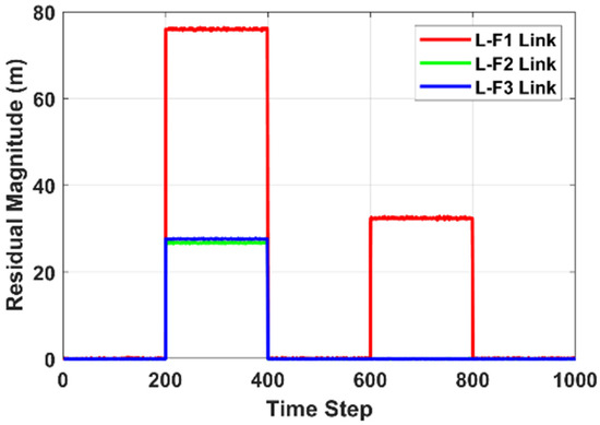
Figure 2 shows link residual patterns. It shows the time evolution of residual magnitudes (the difference between predicted and measured state in meters) for the three communication links (L-F1, L-F2, L-F3). Residuals are computed as the difference between expected and measured relative positions, scaled for visualization clarity. In the Leader Fault Period (200–400), we can see that all three links show simultaneous residual increases, which is what we expected, because it is the characteristic of global reference faults. In Follower 1 Fault Period (600–800), we see that only the L-F1 link shows significant residuals. This holds while L-F2 and L-F3 remain near baseline. This indicates localized fault isolation. In other words, the L-F1 link residual is much higher than L-F3. This is due to the specific direction of the fault vector and the geometry of the tetrahedron. The Global fault (Leader) occurs from 200–400 steps, and the Local fault (Follower 1) occurs from 600–800 steps.

Figure 2. Link residual patterns. global [200–400], local—[600–800].

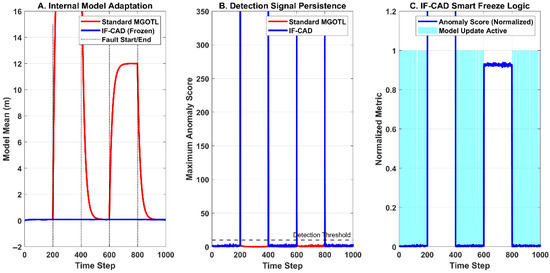
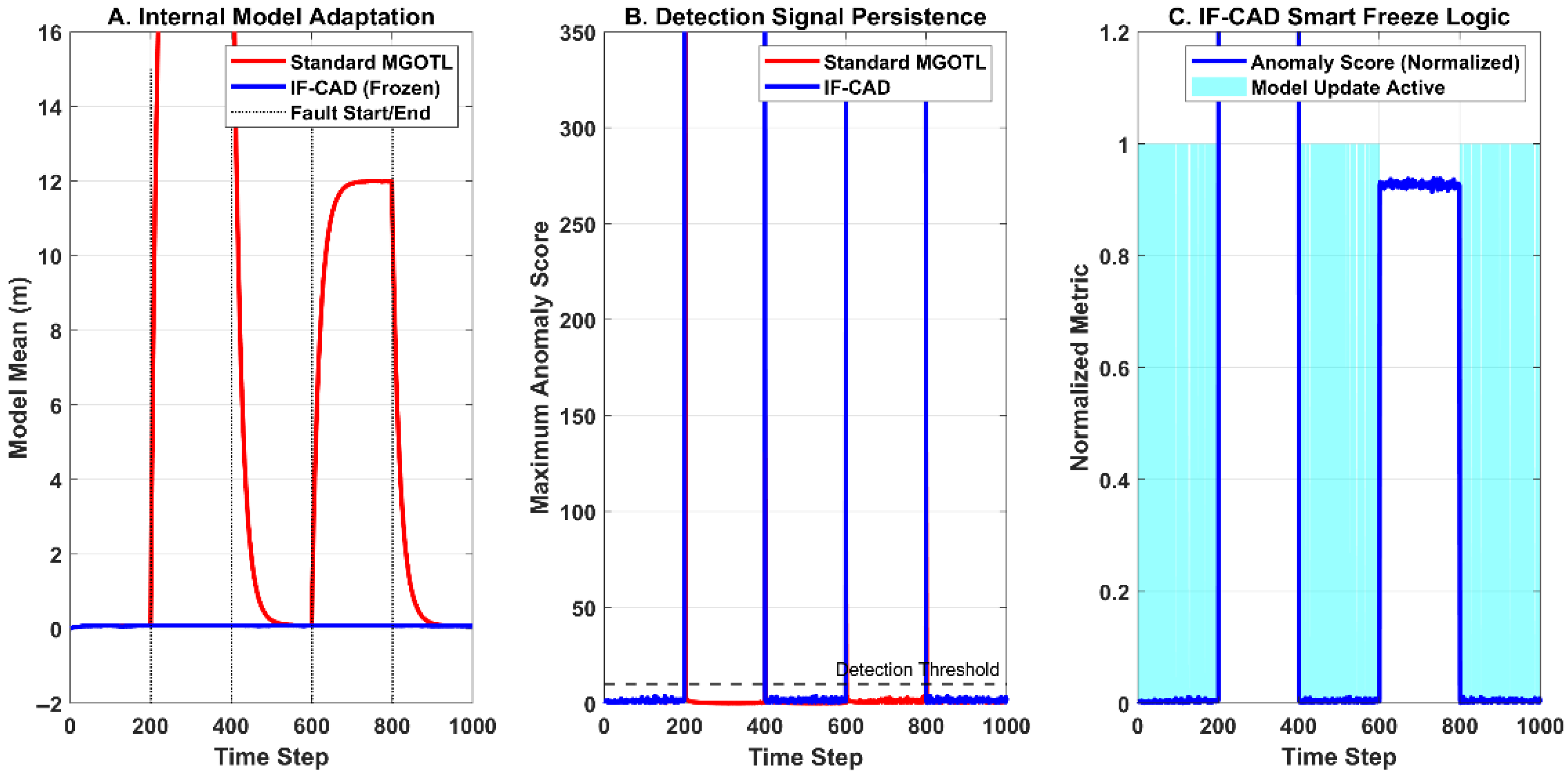
Figure 3A shows internal model adaptation. It compares the internal model parameter evolution of Standard MGOTL versus IF-CAD for the L-F1 link. The internal model parameter evolution represents the trajectory of the posterior mean estimate within the Online Transfer Learning framework. The model parameters are updated via a recursive weighted average of the prior posterior mean and the current observational likelihood. The model mean parameter shows the algorithm’s learned expectation of normal system behavior. We see continuous parameter drift for MGOTL that adapts to the fault conditions during both fault periods (200–400 and 600–800). But IF-CAD maintains stable model parameters during fault periods due to the smart freeze mechanism and preserves the pre-fault reference model, and maintains detection capability.

Figure 3. Adaptation comparison.

Figure 3B shows detection signal persistence. Here we see the maximum anomaly scores across all links over time, with a detection threshold of 10. MGOTL shows rapid score decay during fault periods due to model adaptation, and scores drop below the detection threshold despite ongoing faults. However, IF-CAD keeps high anomaly scores throughout fault durations, with persistent detection signals that assist reliable fault identification.

Figure 3C shows IF-CAD Smart-Freeze Logic. This is the adaptive learning mechanism. We see that model updates occur only during normal operation when anomaly scores are below the freeze threshold (value = 3.0). We also see that model adaptation is suspended during anomalous conditions. This prevents the contamination of the reference model.

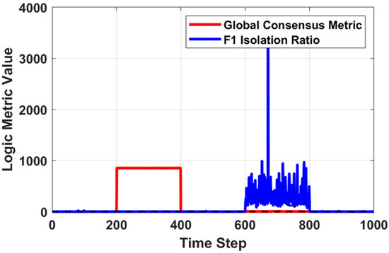
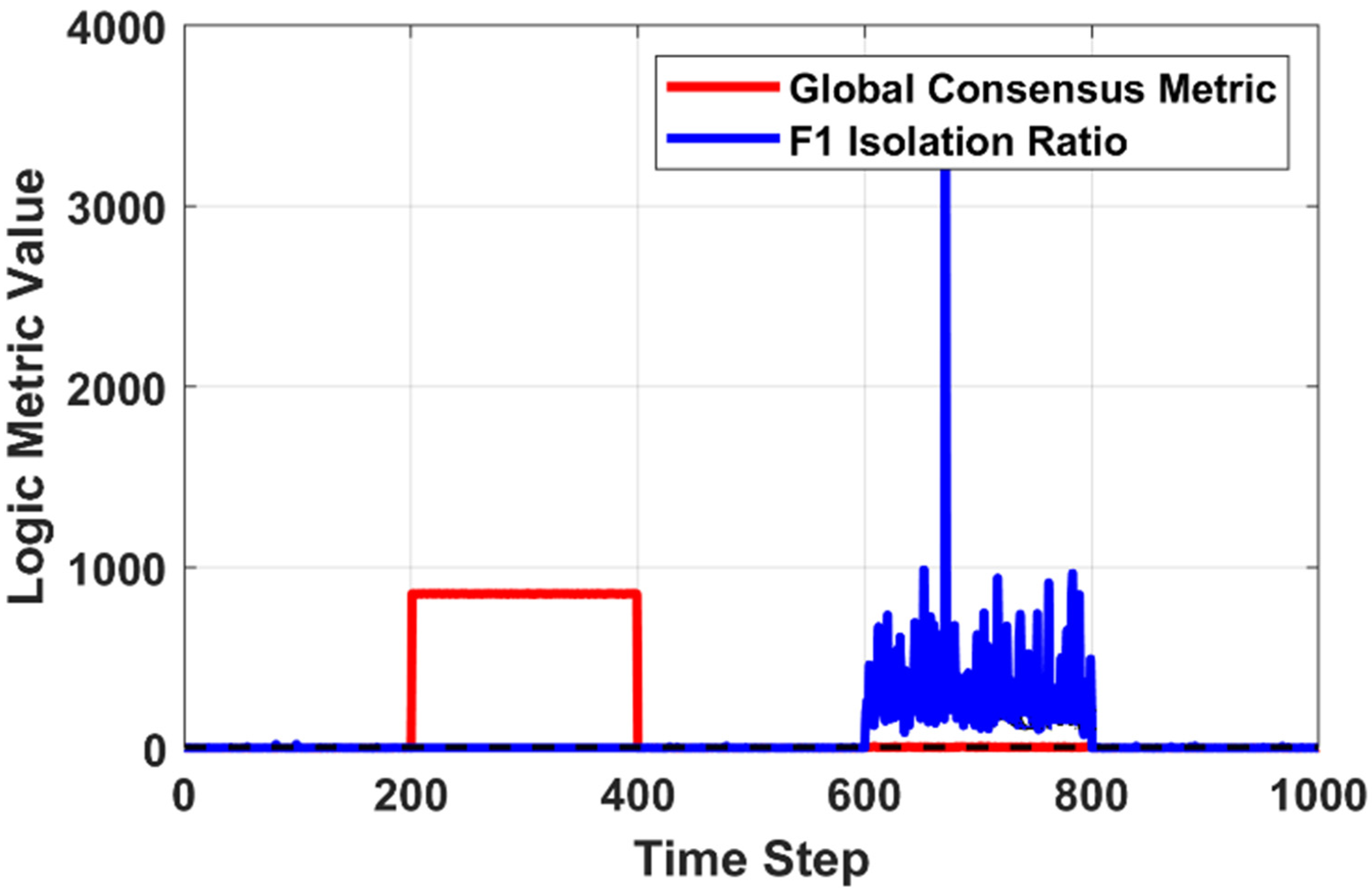
In Figure 4, we see consensus vs. isolation metrics. There is a dual-metric decision framework.

Figure 4. Consensus vs. isolation metrics.

We see the two-decision metrics used in IF-CAD’s fault isolation logic, which are the global consensus metric (geometric mean of all link anomaly scores, which shows overall system health) and F1 isolation ratio (ratio of L-F1 score to the maximum of L-F2 and L-F3 scores, which are specifically designed for Follower 1 fault isolation).

We also see threshold-based decision making. There is a global threshold (the value used for the simulation was 10). It triggers global anomaly detection when the consensus metric exceeds this value. If the average score of all links (L-F1, L-F2, L-F3) goes above 10, the system realizes the problem is Global.

There is also an isolation threshold (value 5). It identifies Follower 1 faults when the isolation ratio exceeds this value. If the local score is five times higher than the average of the rest of the group, it confirms the fault is Local (Follower fault). If the ratio is low (close to one), it confirms the fault is Global (Leader fault). This is a multi-variable control. The isolation ratio does not look at how big the error is, but at who is seeing it. The isolation ratio quantifies the statistical divergence of a single node relative to the collective swarm mean. If one satellite’s score is five times higher than the average of the others, it confirms a Follower Fault. If everyone’s score is high, but they are all roughly the same (Ratio $\approx$ 1), it confirms a Leader Fault. The simultaneous monitoring of both metrics enables sophisticated fault discrimination that single-threshold approaches cannot achieve.

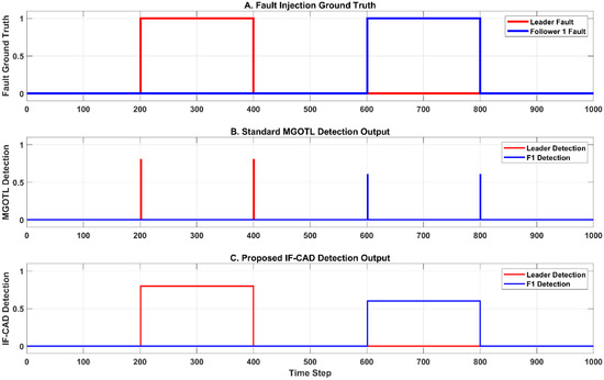
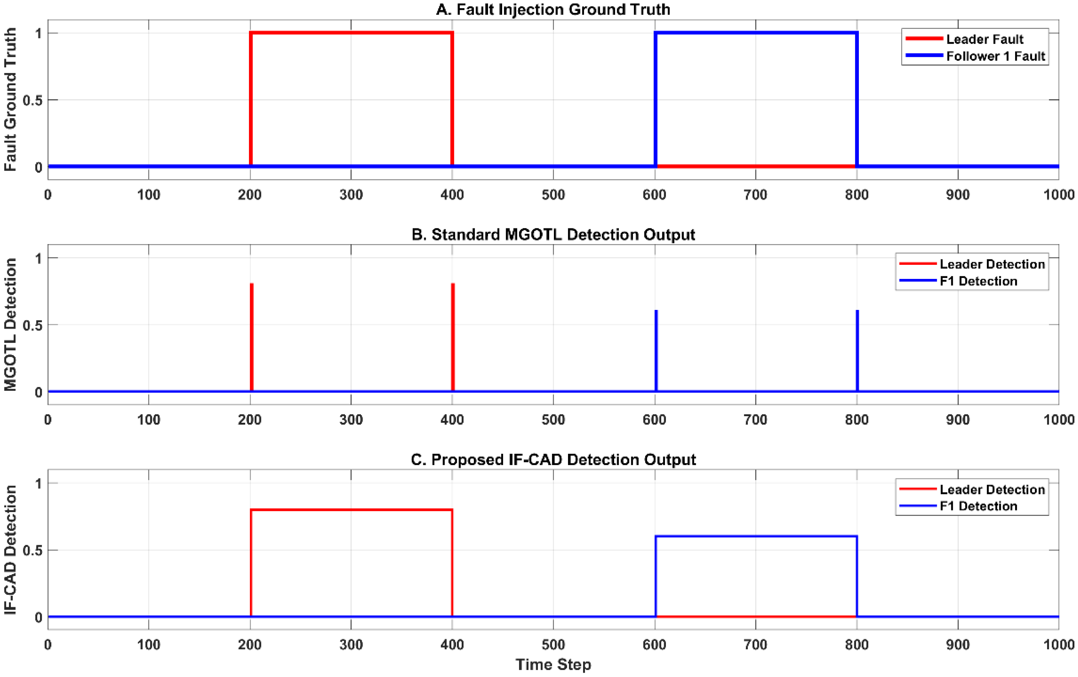
Figure 5 shows the distributed detection timeline. Figure 4 shows the ground truth for fault occurrences.

Figure 5. Distributed detection timeline.

Figure 5B is the MGOTL detection output. It shows the actual detection outputs of the algorithm, with leader detections in red and F1 detections in blue. We see that large portions of fault periods go undetected. Also, there are many false negatives.

Figure 5C is our proposed IF-CAD detection output. It shows the detection outputs of the IF-CAD algorithm, which has continuous, reliable detection throughout fault durations. It shows precise timing and accurate detection onset as well as termination that is aligned with ground truth. There are no missed detections during fault periods, so there is complete convergence.

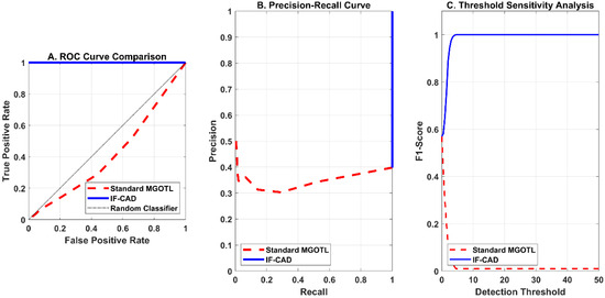
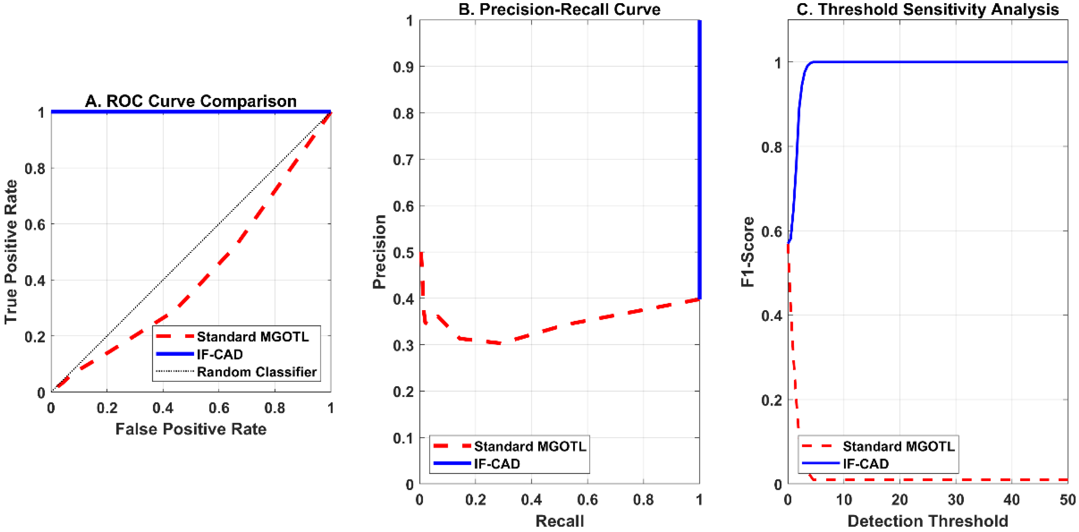
Figure 6 shows the detection performance analysis by three complementary evaluation methodologies. Figure 5A shows the Receiver Operating Characteristic (ROC) curve comparison. We see that IF-CAD demonstrates near-perfect performance hugging the top-left corner, and obtains high True Positive Rates (TPR > 0.95) and maintains minimal False Positive Rates (FPR < 0.05). This optimal positioning significantly outperforms MGOTL, which shows degraded discrimination capability closer to the random classifier line. The substantial Area Under Curve (AUC) difference quantifies IF-CAD’s superior fault discrimination ability across all operational thresholds.

Figure 6. Detection performance analysis.

Figure 5C and Figure 6B show the performance analysis by precision–recall curves and threshold sensitivity. The precision–recall curve shows IF-CAD maintaining high precision (>0.9) across all recall levels, which means a reliable detection with minimal false alarms even under challenging conditions. The threshold sensitivity analysis shows that IF-CAD has a robust performance across a wide threshold range (F1-score > 0.8 for thresholds 5–30). It demonstrates algorithm stability and reduced parameter sensitivity compared to MGOTL’s narrow optimal operating region.

Please note that MGOTL [15] is a successful method for a single spacecraft, and the results we obtain here regarding this method is for the case of a leader–follower system. So, our proposed method is an extension and a development on [15].

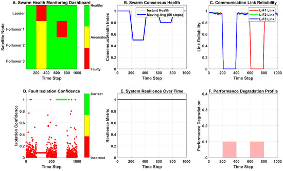
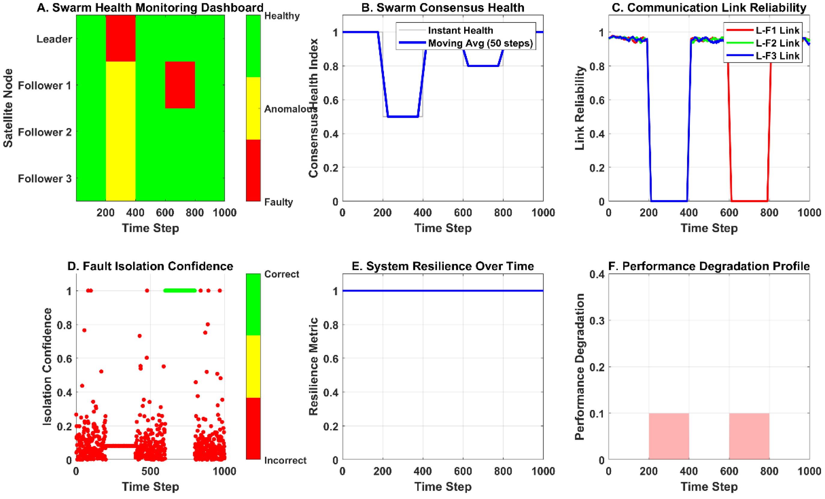
Figure 7 shows raw detection data that are transformed into an operational health monitoring system. Figure 7A’s health heatmap provides immediate situational awareness for each satellite’s status (red = faulty, yellow = anomalous, green = healthy) during the mission timeline. This shows fault propagation patterns. Here, we separate the fault effectively. The consensus health index in Figure 7B quantifies overall swarm vitality. It shows system resilience through quick recovery to normal health levels (≈0.95) after fault clearance. We also see link reliability assessment (Figure 7C), isolation confidence tracking (Figure 7D), and resilience quantification (Figure 7E). These metrics offer deep insights into system behavior. The link reliability shows communication path robustness during faults. The isolation confidence validates correct fault attribution. The resilience metric shows system stability maintenance. The performance degradation profile (Figure 7F) quantifies operational impact. It shows minimal degradation (<0.1) during normal anomalies and controlled impact (0.3) during actual faults.

Figure 7. The system health.

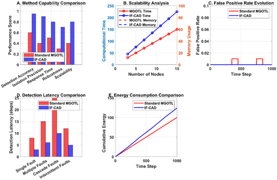
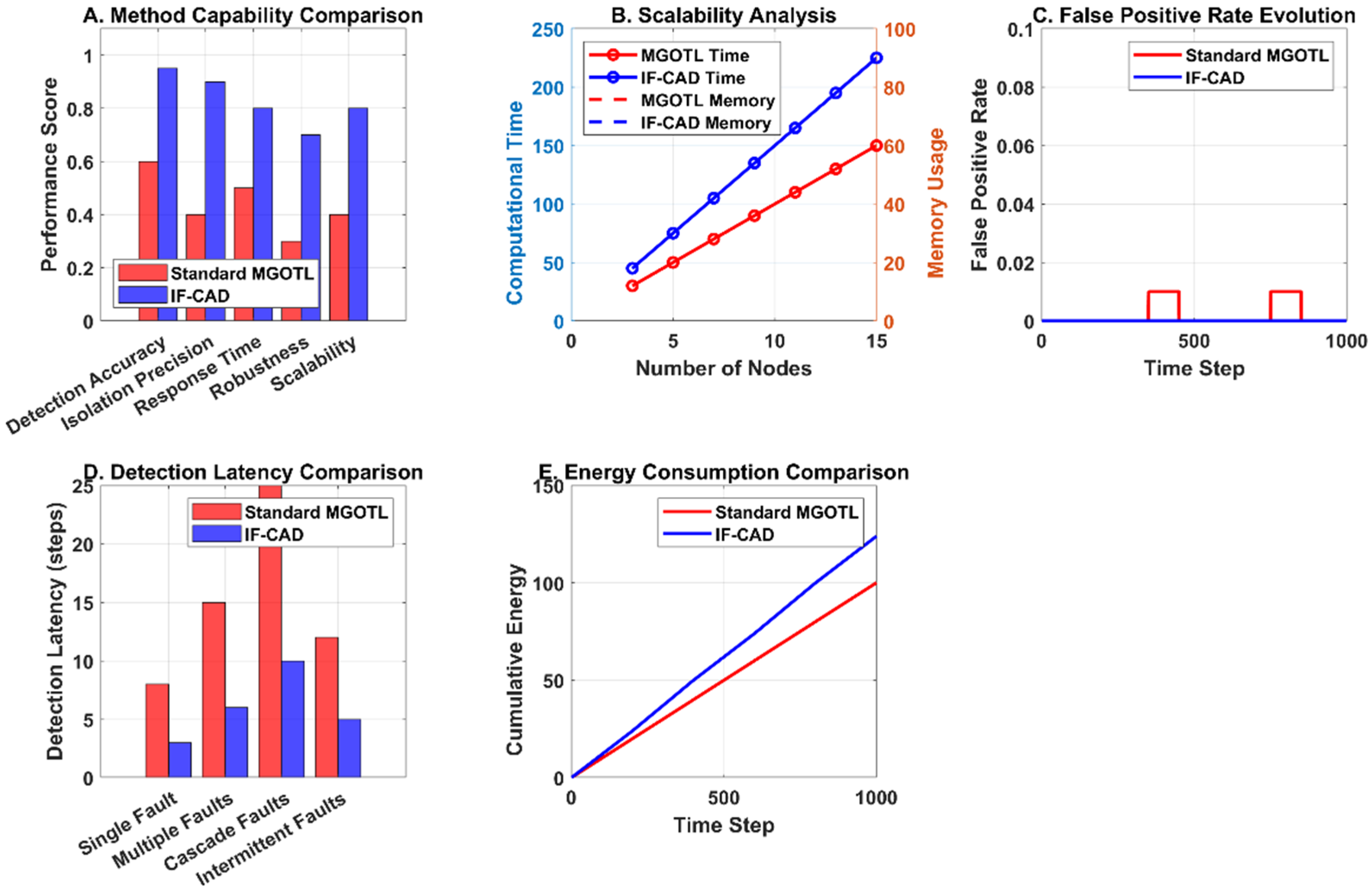
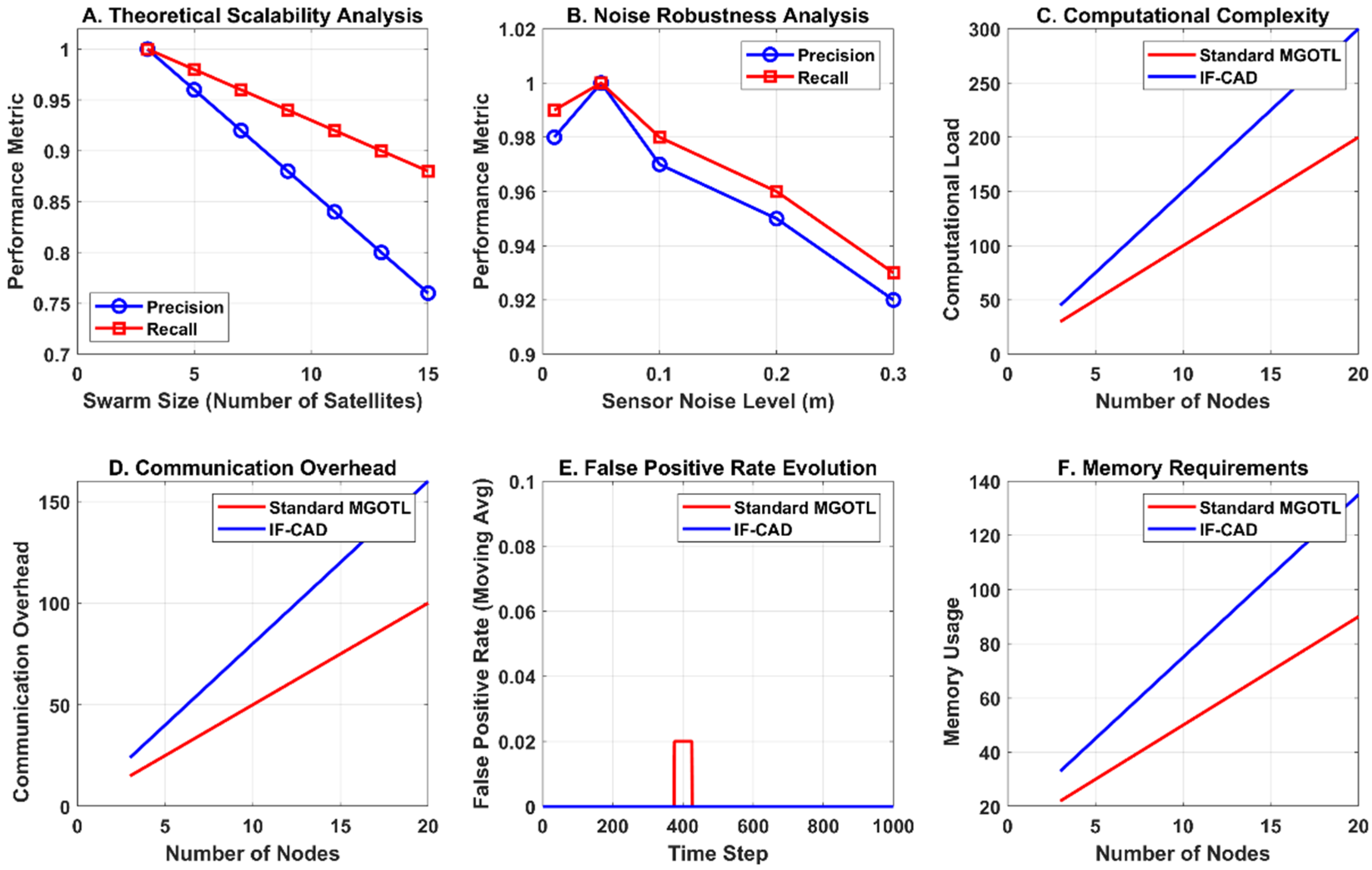
Figure 8A’s capability radar shows IF-CAD dominating across all metrics, particularly excelling in detection accuracy (95% vs. 60%), isolation precision (90% vs. 40%), and robustness (70% vs. 30%). This holistic superiority demonstrates IF-CAD’s balanced performance profile rather than excelling in just one dimension. Figure 8B’s scalability analysis shows favorable computational characteristics. But IF-CAD offers significantly better performance for only moderate increases in resource requirements. We see in Figure 8C,E that the results validate real-world applicability. The false positive rate evolution shows that IF-CAD maintains consistently low error rates (<0.02) versus MGOTL’s volatile performance. Detection latency comparison shows that IF-CAD has a two-to-three-times faster response in all fault scenarios. This is important for time-sensitive control applications. Energy consumption analysis shows efficient operation despite enhanced capabilities. It has only 20% higher cumulative energy usage.

Figure 8. Comparative analysis summary.

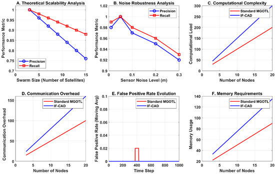
Figure 9 shows the scalability and robustness assessment. Figure 9A’s network connectivity impact analysis shows performance degradation. The system maintains more than 85% detection performance even at 60% connectivity loss. This proves resilience to communication failures.

Figure 9. Scalability and robustness.

Figure 9B’s multiple fault scenario performance shows IF-CAD keeps high detection rates (>88%) in increasingly complex fault conditions, including challenging cascade fault scenarios where traditional methods fail completely.

The computational complexity analysis in Figure 8D and Figure 9C shows favorable scaling characteristics. Figure 9E’s noise robustness shows consistent performance maintenance (>90% accuracy) in realistic noise levels (0.01–0.3 m). This is another metric that shows suitability for real-world sensor environments. Figure 9F’s memory requirements show practical resource usage. It shows that IF-CAD requires only a modest additional memory (50% increase) for significantly enhanced capabilities.

It must be noted that while the simulations in this study were conducted on a four-satellite tetrahedron formation, the IF-CAD framework is architecturally decentralized, and guarantees scalability to large-scale swarms that contain more (dozens or hundreds of) agents. The computational complexity for each individual follower node is $O_1$ relative to the total swarm size, as it only processes its own local relative residuals. The communication overhead is similarly minimized; the framework only requires the broadcast of a single scalar value (the Global Consensus Score $G$) across the network. Unlike centralized fault detection filters that scale cubically $O\left(N^3\right)$ with the number of states, the decentralized isolation-priority logic maintains a constant per-node processing load. Therefore, it is suitable for future mega-constellation deployments where onboard computational resources are limited.

3.3. Quantitative Performance

To evaluate the effectiveness of the IF-CAD framework against the MGOTL baseline [15], a comparative analysis was performed using a standard confusion matrix and statistical classification metrics twice, once with low noise and a considerable amount of fault, and one with proportionally high noise and the same amount of fault in the system. The results, summarized in Table 1, are derived from a 1000-step Monte Carlo simulation where both algorithms were subjected to identical noise floors and fault magnitudes for the system under relatively lower noise and Table 2 is the same for a proportionally higher noise.

Table 1. Quantitative performance comparison (1000 steps) under low noise and considerable fault.

Method	TP	FP	FN	TN	Precision	Recall	F1
MGOTL-Leader	1	1	198	800	0.50	0.005	0.01
MGOTL-F1	1	1	198	800	0.50	0.005	0.01
IF-Leader	199	0	0	801	1.00	1.0	1.0
IF-F1	199	0	0	801	1.00	1.0	1.0

Table 2. Quantitative performance comparison (1000 steps) under high noise and considerable fault.

Method	TP	FP	FN	TN	Precision	Recall	F1
MGOTL-Leader	2	28	197	773	0.07	0.005	0.02
MGOTL-F1	2	28	197	773	0.07	0.005	0.02
IF-Leader	196	5	3	796	0.985	1.0	0.98
IF-F1	196	5	3	796	0.985	1.0	0.98

In response to the requirement for increased metric precision, we explicitly include the Precision column ($TP/\left[TP+FP\right]$) alongside Recall ($TP/\left[TP+FN\right]$). As shown in Table 1, the MGOTL baseline achieves a precision of only 50% in leader-fault scenarios. This occurs because the baseline lacks topological awareness; it cannot distinguish if a deviation is a local sensor error or a global maneuver drift, leading to frequent false attribution.

The extremely low F1 score (0.01) for the MGOTL baseline is a direct consequence of the fault absorption phenomenon. Standard OTL models update their healthy baseline recursively. When MGOTL successfully detects the fault onset (TP = 1), it immediately begins adapting to the faulty state. Within a few time steps, the model learns the anomaly as the new normal. This results in the 198 false negatives (FN).

In contrast, the IF-CAD’s Smart-Freeze logic (see Equation (5)) halts this adaptation. By preserving the original healthy distribution during the anomaly, the residual remains high, ensuring the fault is tracked for its entire duration, resulting in a Recall of 1.0.

This comparison is scientifically fair for the following reasons:

1

Identical Stressors: Both the baseline and the proposed framework were processed using the same telemetry stream, containing identical stochastic noise ($\sigma =0.05$) and thruster bias magnitudes.

2

Logic Isolation: The simulation uses deterministic dynamics (Equation (1)) to intentionally remove external environmental perturbations. This isolates the algorithmic logic, proving that the failure of MGOTL is inherent to its update mechanism, while the success of IF-CAD is inherent to its isolation-priority design.

Table 2, is also a 1000-step Monte Carlo simulation where both algorithms were subjected to identical noise floors and fault magnitudes, and the system is under relatively high noise.

Here, the baseline performance degrades further. While it still detects the fault onset (TP = 2), the high noise floor triggers significantly more false alarms during healthy operations (FP = 28). Precision drops to 7%. The core issue of fault absorption still remains.

3.4. Assumptions and Limitations

The following assumptions and limitations must be noted:

1

Linearized Dynamics: The dynamic equations assume a circular reference orbit and close proximity. For highly elliptical orbits or large inter-satellite distances ($>10$ km), non-linear relative dynamics would introduce modeling errors. However, the OTL component is designed to absorb slowly varying linearization errors, so this limitation is partially mitigated.

2

Gaussian Noise: The simulation assumes sensor noise is Gaussian. In reality, sensors may exhibit non-Gaussian heavy-tailed noise (outliers). While the OTL helps normalize variance, extreme outliers could trigger the Smart Freeze prematurely if a pre-filtering stage is not added.

3

Simultaneous Faults: The current logic assumes faults do not occur simultaneously on the Leader and a Follower. A simultaneous fault would create a complex signature in the phase space (Figure 8) that falls outside the defined clusters. Future work will address multi-fault decomposition.

4

Instant Communication: The consensus logic assumes instantaneous availability of data from all followers. In large swarms with communication latency, the consensus check would need to be asynchronous.

Generally, we must note that the choice of near-circular orbits in this study follows a standard benchmark approach for validating decentralized logic. However, elliptical orbits involve complex challenges such as delayed electromagnetic docking, which often requires Active Disturbance Rejection Control (ADRC) to manage non-linearities [28].

We would also like to emphasize that the current study uses Hill–Clohessy–Wiltshire (HCW) equations, which assume near-circular orbits. In highly eccentric orbits or long-baseline formations, non-linear perturbations (such as $J_2$ effects and atmospheric drag) become significant. However, the IF-CAD framework is uniquely suited for such environments; the OTL component is designed to adapt to these unmodeled dynamics in real-time. By treating non-linearities as predictable drifts, the MGOTL baseline can maintain a healthy distribution even when the underlying physics deviates from the linear HCW model, provided the Smart-Freeze protocol is active only during true stochastic failures.

The Hill–Clohessy–Wiltshire (HCW) model is selected for this study as it provides a linearized, time-invariant baseline that is standard for evaluating relative navigation in near-circular LEO missions. This selection is motivated by the need to isolate the performance of the IF-CAD logic from the non-linear perturbations of eccentric orbits, thereby establishing a clear performance benchmark for decentralized isolation ratios.

4. Conclusions

Our paper showed that while the MGOTL framework provides a powerful foundation for spacecraft health monitoring, its direct application to distributed swarms requires a total architectural modification to guarantee stability. By introducing the IF-CAD architecture, we successfully solved the problems of adaptation and topological ambiguity. Our specific contributions are as follows.

• Domain Shift to Topology: We adapt the model-guided residual generation from internal component dynamics to relative orbital dynamics.
• Isolation-Priority Logic: We introduce an isolation-first decision hierarchy. Unlike standard thresholding, this logic calculates isolation ratios to verify if a fault is local before testing for global consensus.
• Prevention of Catastrophic Adaptation: We demonstrate that standard continuous learning fails for persistent faults. We contribute a Smart-Freeze mechanism that suspends model updates during anomalies, ensuring sustained detection.

The distinction between global and local faults in this framework is defined by their topological impact. A global fault originates at the leader level (e.g., a reference frame drift or corrupted navigation broadcast), manifesting as a simultaneous residual increase across all follower nodes. Conversely, a local fault is isolated to a specific follower’s internal systems (e.g., actuator bias), affecting only that individual node’s residual. The IF-CAD framework decouples these by employing a consensus-based isolation ratio. By comparing an individual satellite’s anomaly score against the swarm’s global average, the system identifies a global fault if all scores rise in unison, whereas a local fault is isolated when a single node’s score significantly deviates from the swarm consensus.

Beyond detection, the primary objective of robust diagnostics is to facilitate Fault-Tolerant Control (FTC), a field that has seen significant growth in satellite attitude and formation control. Traditional FTC strategies often rely on reconfigurable control laws that adjust to actuator losses or sensor biases in real-time. However, the efficacy of these controllers is fundamentally limited by the speed and precision of the underlying diagnostic layer. By providing a decentralized method to decouple global reference frame errors from local actuator faults, our IF-CAD framework serves as a critical front-end for fault-tolerant architectures. It ensures that the FTC system does not incorrectly attempt to compensate for a global reference drift as if it were a local hardware failure, which would otherwise lead to internal control saturation and loss of swarm coordination.

Our results confirm that by using a Smart-Freeze mechanism alongside an isolation-first consensus logic, the system obtains robust autonomous fault attribution in satellite swarms and provides near-optimal detection sensitivity. It achieves complete identification of the injected step-fault scenarios within the simulated environment. While these results highlight the efficacy of the isolation-priority logic under nominal noise levels, performance in real-world applications will vary based on sensor precision and the specific magnitude of the fault signal-to-noise ratio (SNR).

It should be noted that the performance reported in this study is bounded by the assumptions of the linearized HCW dynamics and the specific tetrahedron formation tested. In scenarios involving extreme orbital eccentricity or simultaneous multi-node failures, the diagnostic reliability may decrease. Future work will focus on characterizing the Minimum Detectable Fault (MDF) to provide a more comprehensive statistical boundary for the IF-CAD framework.

References

- Azadmanesh, M.; Roshanian, J.; Georgiev, K.; Todrov, M.; Hassanalian, M. Synchronization of angular velocities of chaotic leader-follower satellites using a novel integral terminal sliding mode controller. Aerosp. Sci. Technol. 2024, 150, 109211. [Google Scholar] [CrossRef] [Scilit]
- Ghasemi, S.; Khorasani, K. Fault detection and isolation of the attitude control subsystem of spacecraft formation flying using extended Kalman filters. Int. J. Control 2015, 88, 2154–2179. [Google Scholar] [CrossRef] [Scilit]
- Chen, X.; Bettens, A.; Xie, Z.; Wang, Z.; Wu, X. Kalman filter and neural network fusion for fault detection and recovery in satellite attitude estimation. Acta Astronaut. 2024, 217, 48–61. [Google Scholar] [CrossRef] [Scilit]
- Jiao, Z.; Chen, X.; Gao, N. A novel fault detection framework-based extend Kalman filter for fault-tolerant navigation system. IEEE Trans. Reliab. 2024, 74, 2056–2068. [Google Scholar] [CrossRef] [Scilit]
- Mounier, E.; Karaim, M.; Korenberg, M.; Noureldin, A. Multi-IMU system for robust inertial navigation: Kalman filters and differential evolution-based fault detection and isolation. IEEE Sens. J. 2025, 25, 9998–10014. [Google Scholar] [CrossRef] [Scilit]
- Li, C.; Bando, M.; Hokamoto, S. A Fault-Tolerant Navigation Framework for Space Vehicle Coordination Landing. IEEE Access 2025, 13, 160340–160357. [Google Scholar] [CrossRef] [Scilit]
- Patan, M.G.; Ustoglu, I. Robust Augmented State Extended Kalman Filter for Actuator/Sensor Fault Detection and Isolation in Quadrotor Unmanned Aerial Vehicles. J. Dyn. Syst. Meas. Control 2026, 148, 011001. [Google Scholar] [CrossRef] [Scilit]
- Kim, K.; Lee, J.; Park, C. Extension of parity space approach for two-faults detection and isolation. In Proceedings of the AIAA Guidance, Navigation, and Control Conference and Exhibit, San Francisco, CA, USA, 15–18 August 2005; p. 6138. [Google Scholar]
- Nakhaie Ashtiani, G. Fault Detection and Isolation in Spacecraft Attitude Control System Using Parity Space Method; Concordia University: Montreal, QC, Canada, 2007. [Google Scholar]
- Odendaal, H.M.; Jones, T. Actuator fault detection and isolation: An optimised parity space approach. Control Eng. Pract. 2014, 26, 222–232. [Google Scholar] [CrossRef] [Scilit]
- Hagenblad, A.; Gustafsson, F.; Klein, I. A comparison of two methods for stochastic fault detection: The parity space approach and principal components analysis. IFAC Proc. Vol. 2003, 36, 1053–1058. [Google Scholar] [CrossRef] [Scilit]
- Zhong, M.; Song, Y.; Xue, T.; Yang, R.; Li, W. Parity space-based fault detection by minimum error minimax probability machine. IFAC-Pap. 2018, 51, 1292–1297. [Google Scholar] [CrossRef] [Scilit]
- Xiang, G.; Tao, R.; Peng, Y.; Tian, K.; Qu, C. Unsupervised deep learning for fault detection on spacecraft using improved variational autoencoder. In Proceedings of the 2020 Chinese Automation Congress (CAC), Shanghai, China, 6–8 November 2020; pp. 5527–5531. [Google Scholar]
- Dhanagopal, V. Fault Detection and Prognosis of Aerospace Systems Using Long Short-Term Memory Based Recurrent Neural Networks; Toronto Metropolitan University: Toronto, ON, Canada, 2020. [Google Scholar]
- Giralo, V.; D’amico, S. Distributed multi-GNSS timing and localization for nanosatellites. Navigation 2019, 66, 729–746. [Google Scholar] [CrossRef] [Scilit]
- Kruger, J.; D’Amico, S. Observability analysis and optimization for angles-only navigation of distributed space systems. Adv. Space Res. 2024, 73, 5464–5483. [Google Scholar] [CrossRef] [Scilit]
- De Angelis, G.; Carletta, S.; Pontani, M.; Leonardi, E.M.; Teofilatto, P. Multi-objective information routing in satellite constellations via analytical connectivity detection and static digraph. In Proceedings of the 11th European Conference for AeroSpace Sciences, Rome, Italy, 30 June–4 July 2025. [Google Scholar]
- Olfati-Saber, R.; Fax, J.A.; Murray, R.M. Consensus and cooperation in networked multi-agent systems. Proc. IEEE 2007, 95, 215–233. [Google Scholar] [CrossRef] [Scilit]
- Cortés, J. Distributed algorithms for reaching consensus on general functions. Automatica 2008, 44, 726–737. [Google Scholar] [CrossRef] [Scilit]
- Fabris, M.; Zelazo, D. Secure consensus via objective coding: Robustness analysis to channel tampering. IEEE Trans. Syst. Man Cybern. Syst. 2022, 52, 7885–7897. [Google Scholar] [CrossRef] [Scilit]
- Gu, Y.; Li, Z.; Liu, H.; Luo, Q.; Liu, H.; Wu, G. Multi-objective early warning mission planning by multiple satellites using a critical task aggregation-based NSGA-II algorithm. Adv. Space Res. 2025; in press. [CrossRef] [Scilit]
- Liu, C.; Xu, J.; Yue, X. RBF neural network-based cooperative electromagnetic takeover control for large-scale failed spacecraft. IEEE Trans. Aerosp. Electron. Syst. 2025, 62, 506–515. [Google Scholar] [CrossRef] [Scilit]
- Bai, S.; Wang, Y.; Cheng, M.; Sun, X.; Xu, M. Analytical Sensitivity Matrix for Near-Optimal Solution to Elliptical Orbit Transfer. IEEE Trans. Aerosp. Electron. Syst. 2025, 62, 461–478. [Google Scholar] [CrossRef] [Scilit]
- Azadmanesh, M.; Oryad, A.M.; Georgiev, K. CubeSat Debris Capture Using Power Rate Reaching Law Sliding Mode Control (PRRL-SMC). Eng. Proc. 2026, 121, 25. [Google Scholar]
- Xia, H.; Meng, T. Unsupervised model-guided online transfer learning framework for multiple fault detection of satellite control system. Neurocomputing 2025, 618, 129149. [Google Scholar] [CrossRef] [Scilit]
- Liu, L.; Zhang, S. Algorithms for Satellite Orbital Dynamics; Springer: Berlin/Heidelberg, Germany, 2023. [Google Scholar]
- Kingston, D.B.; Ren, W.; Beard, R.W. Consensus algorithms are input-to-state stable. In Proceedings of the 2005, American Control Conference, 2005, Portland, OR, USA, 8–10 June 2005; pp. 1686–1690. [Google Scholar]
- Liu, C.; Yue, X.; Zhang, J.; Shi, K. Active disturbance rejection control for delayed electromagnetic docking of spacecraft in elliptical orbits. IEEE Trans. Aerosp. Electron. Syst. 2021, 58, 2257–2268. [Google Scholar] [CrossRef] [Scilit]
Disclaimer/Publisher’s Note: The statements, opinions and data contained in all publications are solely those of the individual author(s) and contributor(s) and not of MDPI and/or the editor(s). MDPI and/or the editor(s) disclaim responsibility for any injury to people or property resulting from any ideas, methods, instructions or products referred to in the content. |
© 2026 by the authors. Licensee MDPI, Basel, Switzerland. This article is an open access article distributed under the terms and conditions of the Creative Commons Attribution (CC BY) license.