Research on Fatigue Crack Growth Rate Prediction of 2024-T3 Aluminum Alloy Friction Stir Welded Joints Driven by Machine Learning

Abstract

Fatigue crack propagation in friction stir welded joints significantly affects aircraft structural integrity. This study investigates the influence of welding speed, rotational speed, specimen thickness, loading frequency, and stress ratio on the fatigue crack growth rate. Four classical machine learning models with different structures—Deep Back-Propagation Network, Random Forest, Support Vector Regression, and K-Nearest Neighbors—were employed to predict fatigue crack growth behavior. The results show that all models achieve strong predictive performance. For FSWed joints, Deep BP and KNN exhibit comparable performance (R² > 0.98) on the training data, indicating similar learning capabilities with sufficient data coverage. Notably, KNN achieves the fastest training time (<0.3 s), while all models require less than 5 s of computation time. These results demonstrate that machine learning-based models provide an efficient and reliable alternative for rapid fatigue crack growth evaluation, supporting damage-tolerant design and structural integrity assessment in aircraft engineering.

1. Introduction

As a solid-state joining technique, friction stir welding (FSW) avoids large fusion welding defects and reduces deformation under lower heat input [1]. The 2024-T3 aluminum alloy is widely utilized in aircraft structures, such as skins, wings, and frames, due to its low density, high strength, and stiffness [2,3]. Structural safety is paramount for aircraft performance, and fatigue failure constitutes the primary damage mechanism for critical load-bearing components [4,5]. Therefore, studying the fatigue crack growth rate in 2024 FSWed joints is vital for improving the accuracy and reliability of fatigue life predictions in aircraft structures.

The stress-life (S-N) method and the damage-tolerant approach are primary approaches for modeling fatigue properties and designing for fatigue resistance [6]. The S-N curve approach does not capture the behavior of fatigue crack propagation, such as crack growth rate and stress intensity at different stages—factors that are crucial for understanding fatigue crack behavior [7,8]. To address this limitation, the damage-tolerant approach has been developed. In this approach, da/dN-ΔK curves are commonly used to investigate crack growth from initial flaws to final failure, based on experimental data and principles of fracture mechanics [9].

Fatigue crack growth rate (FCGR) is influenced by numerous factors, among which welding speed and rotational speed are the most critical, as they directly determine the residual stress distribution during the welding process [10]. Due to the intense local thermo-mechanical coupling during the FSW process, significant residual stresses are generated in the weld [11,12]. Tensile residual stresses promote crack opening, thereby accelerating the FCGR. Conversely, compressive residual stresses reduce the tensile stress at the crack tip, increasing the applied stress required for propagation. Consequently, cracks advancing through compressive residual stress fields exhibit reduced growth rates.

It has been well established in previous studies that the relationship between welding speed and residual stress is nonlinear [13,14]. At lower welding speeds, frictional heating dominates, and residual stress tends to decrease as the welding speed increases. At higher welding speeds, the heat generated by plastic deformation becomes dominant, causing residual stress to increase with welding speed. However, when the welding speed continues to increase beyond a certain point, the overall heat input begins to decline, leading to a corresponding decrease in residual stress. Additionally, welding speed determines the heat input per unit length of the weld. At lower welding speeds, the heat input per unit length increases, which helps to reduce the extent of uneven heating in the weld zone and mitigates asynchronous thermal expansion between different regions during the cooling process. Compared to welding speed, the rotational speed of the stirring head has a more pronounced effect on the residual stress distribution within the welded joint [10]. A higher rotational speed increases the input power during welding, thereby elevating the specimen temperature and enhancing the stirring and mixing of material around the tool [15,16].

In fatigue analysis, an increase in the thickness of the welding plate will reduce the effective area of the plate cross-section, decrease the stress amplitude per unit cross-sectional area under cyclic loading, and thereby reduce the FCGR of the welded structure [17,18]. In addition, the stress ratio R is defined as the ratio of minimum to maximum stress within a loading cycle, and it can significantly influence crack growth behavior. It has been shown that the fatigue crack growth rate tends to increase with increasing stress ratio [19,20]. For the frequency, Musuva [21] indicated that frequency has minimal influence on crack growth rates at low stress ratios. However, at high stress ratios, lower loading frequencies may lead to increased crack growth rates.

Previous studies indicate that the factors affecting the FCGR in friction stir welded structures are numerous and complex, making accurate prediction challenging using traditional methods. In recent years, with the increasing accessibility of experimental data, many researchers have explored the use of machine learning (ML) models to accelerate FCGR prediction [1,22,23,24,25]. Kamble [26] proposed an ML-based approach for predicting FCGR in steel, successfully modeling crack growth in compact tension (CT) specimens with varying geometries and subjected to different cyclic loading conditions. Wang [27] emphasized that the performance of ML algorithms heavily depends on the adequacy of experimental data, which should capture the nonlinear relationships across the full range of ΔK and R. Fang [28] compared three ML methods and found that the Gaussian Process surrogate model achieved the highest prediction accuracy, Particle Swarm Optimization, which is based the Back-Propagation Neural Network, exhibited the best extrapolation capability, and the General Regression Neural Network performed well in terms of training efficiency.

In FCGR prediction modeling, different ML algorithms exhibit distinct characteristics and performance across various dimensions, including prediction accuracy, generalization ability, noise robustness, training efficiency, and interpretability. The Deep Back-Propagation (Deep BP) Network offers strong nonlinear fitting and multivariate learning capabilities. When provided with sufficient training data, it can achieve highly accurate predictions. Random Forest (RF) generates robust results by aggregating multiple decision trees. It demonstrates excellent generalization and noise resistance, particularly for small-to-medium-sized datasets, and frequently yields high prediction accuracy. Support Vector Regression (SVR) employs kernel functions to capture nonlinear relationships in crack propagation behavior. By leveraging the principle of maximum margin, SVR effectively controls model complexity and delivers good generalization and accuracy, even with limited datasets. The K-Nearest Neighbors (KNN) algorithm, based on instance, makes predictions by evaluating similarity to neighboring data points. It is simple, does not require explicit training, and can produce reliable results when the data space is densely sampled locally.

In view of the above considerations, fatigue crack growth in FSWed joints remains a challenging problem due to the strong coupling among welding process parameters, material characteristics, and loading conditions. Classical fracture mechanics-based models describe crack growth primarily through the ΔK, and often require additional assumptions and repeated recalibration when welding parameters, specimen geometry, or loading conditions vary. This limits their applicability in practical engineering scenarios involving heterogeneous welded structures. To address these limitations, the present study proposes a systematic, data-driven framework for FCGR prediction in FSWed joints under multi-parameter coupled conditions. Rather than treating ΔK as the sole governing variable, the framework explicitly incorporates welding speed, rotational speed, specimen thickness, loading frequency, and stress ratio as additional explanatory inputs, enabling the quantification of their combined and nonlinear influence on the FCGR. Four representative machine learning algorithms—Deep Back-Propagation, Random Forest, Support Vector Regression, and K-Nearest Neighbors—are implemented and comparatively evaluated using a comprehensive literature-compiled dataset.

The main contribution of this work lies in demonstrating that reliable and computationally efficient FCGR prediction can be achieved by integrating fracture mechanics-based driving parameters with welding and loading variables within a unified machine learning framework. This approach provides new insight into the relative role of process and loading conditions in fatigue crack growth and offers a practical pathway for data-driven fatigue assessment of welded aerospace structures.

2. Data Description

To develop the ML models, relevant experimental FCGR data for the 2024-T3 aluminum alloy were collected from the author’s previous work and relevant published studies. FCGR experiments were conducted in accordance with the ASTM E647 standard using compact tension (C(T)) specimens. Table 1 displays the chemical compositions of the 2024-T3 alloy. The dataset includes FCGR measurements for both the base material (BM) and FSWed joints under varying specimen thicknesses, rotational speeds, welding speeds, loading frequencies, and stress ratios, comprising a total of 38 test sets and 1572 data points, as shown in Table 2. Within this dataset, the influence parameters for the base material include specimen thickness, loading frequency, stress ratio, and the stress intensity factor range (ΔK), with a total of 576 data points. However, for the FSWed joints, the influence variables include specimen thickness, rotational speed, welding speed, loading frequency, stress ratio, and ΔK, totaling 996 data points. The FCGR is reported in mm/cycle, while the stress intensity factor range ΔK is expressed in MPa·m^1/2.

Table 1. Chemical compositions of the 2024-T3 alloy.

Material	Chemical Composition (%)
2024-T3	Cu	Si	Fe	Mn	Mg	Zn	Cr	Ti	Al
	3.8–4.9	0.5	0.5	0.3–0.9	1.2–1.8	0.25	0.1	0.15	Base

Table 2. FCGR dataset for 2024-T3 under base material and friction stir welded conditions.

Number	Material	Thickness (mm)	Rotational Speed (rpm)	Welding Speed (mm/min)	Loading Frequency	Stress Ratio	Data Source
1	BM	8	/	/	20	0.1	Ref. [29]
2	BM	8	/	/	10	0.1	Ref. [30]
3	BM	4	/	/	15	0.1	Ref. [14]
4	BM	4	/	/	20	0.1	Ref. [31]
5	BM	4	/	/	20	0.1	Ref. [31]
6	BM	4	/	/	10	0.06	Ref. [32]
7	BM	3.5	/	/	10	0.1	Ref. [33]
8	BM	3.2	/	/	60	0.5	Ref. [34]
9	BM	3	/	/	11	0.1	Ref. [35]
10	BM	3	/	/	11	0.1	Ref. [36]
11	BM	3	/	/	11	0.1	Ref. [37]
12	BM	2	/	/	10	0.1	Ref. [38]
13	BM	0.1	/	/	10	0.1	Ref. [39]
14	BM	0.1	/	/	10	0.7	Ref. [39]
15	FSW	8	200	150	20	0.1	Ref. [29]
16	FSW	8	400	150	20	0.1	Ref. [29]
17	FSW	8	800	31.5	10	0.1	Ref. [30]
18	FSW	8	630	25	10	0.1	Ref. [30]
19	FSW	8	500	16	10	0.1	Ref. [30]
20	FSW	8	400	8	10	0.1	Ref. [30]
21	FSW	6	931	70	10	0.1	Ref. [40]
22	FSW	5	931	70	10	0.5	Ref. [2]
23	FSW	4	700	110	15	0.1	Ref. [14]
24	FSW	4	900	110	15	0.1	Ref. [14]
25	FSW	4	1100	110	15	0.1	Ref. [14]
26	FSW	4	1300	110	15	0.1	Ref. [14]
27	FSW	4	1500	110	15	0.1	Ref. [14]
28	FSW	4	1100	70	15	0.1	Ref. [14]
29	FSW	4	1100	90	15	0.1	Ref. [14]
30	FSW	4	1100	130	15	0.1	Ref. [14]
31	FSW	4	1100	150	15	0.1	Ref. [14]
32	FSW	4	700	200	20	0.1	Ref. [31]
33	FSW	4	700	200	20	0.1	Ref. [31]
34	FSW	4	1000	100	10	0.06	Ref. [32]
35	FSW	3.5	1180	47.5	10	0.1	Ref. [33]
36	FSW	3	1450	12	11	0.1	Ref. [35]
37	FSW	3	1450	30	61	0.1	Ref. [36]
38	FSW	2	1200	300	10	0.1	Ref. [38]

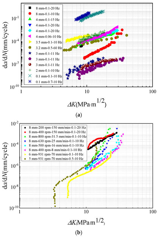
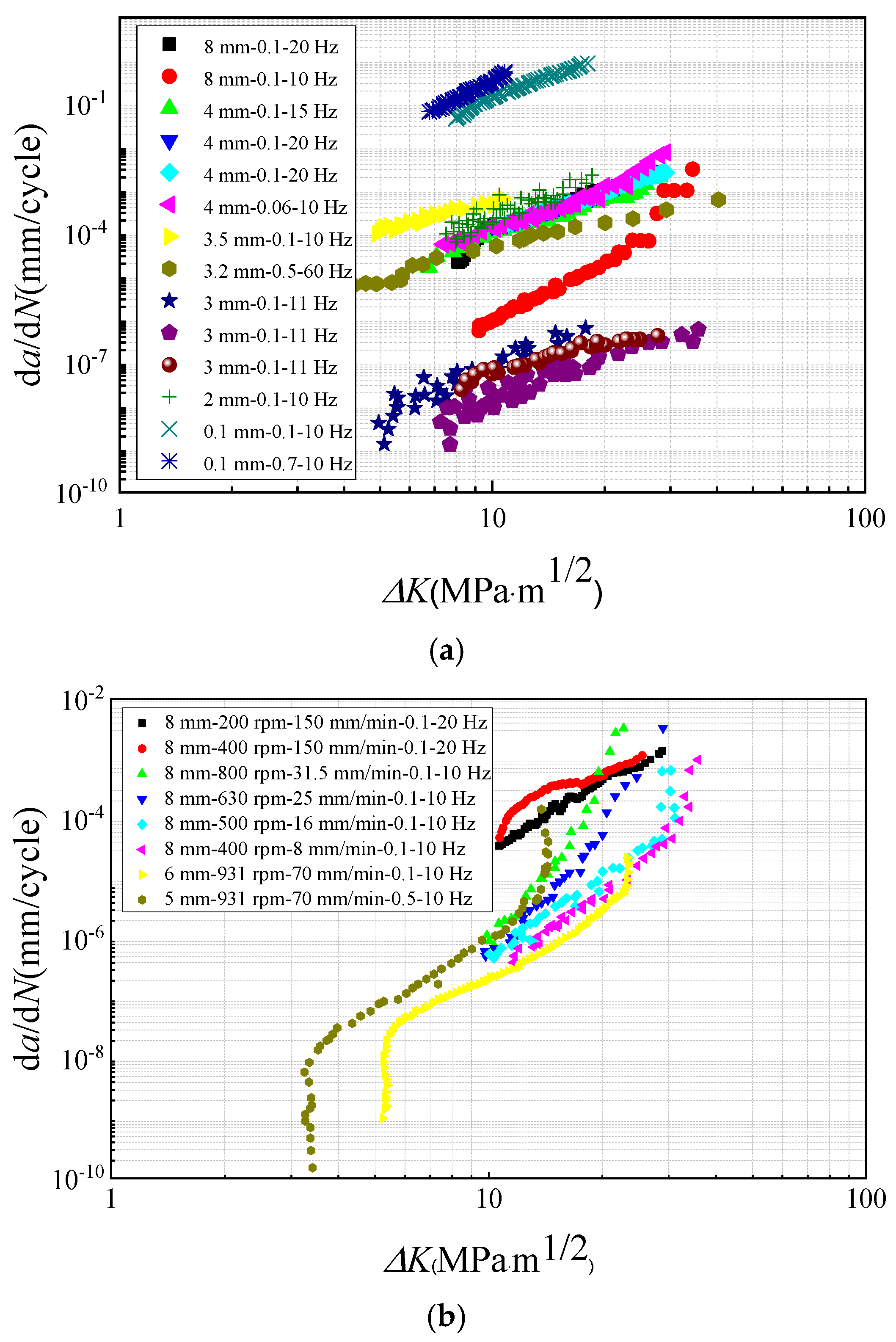
Figure 1 presents the experimental data of the FCGR for FSWed joints under various conditions. Figure 1a compares the FCGR behavior of the base material specimens with different thicknesses. It can be observed that, when the loading frequency and stress ratio are held constant, the FCGR decreases as the specimen thickness increases. This trend is attributed to the enhanced crack-tip constraint and higher resistance to plastic deformation in thicker specimens, which collectively suppress crack propagation.

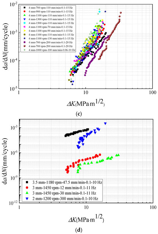
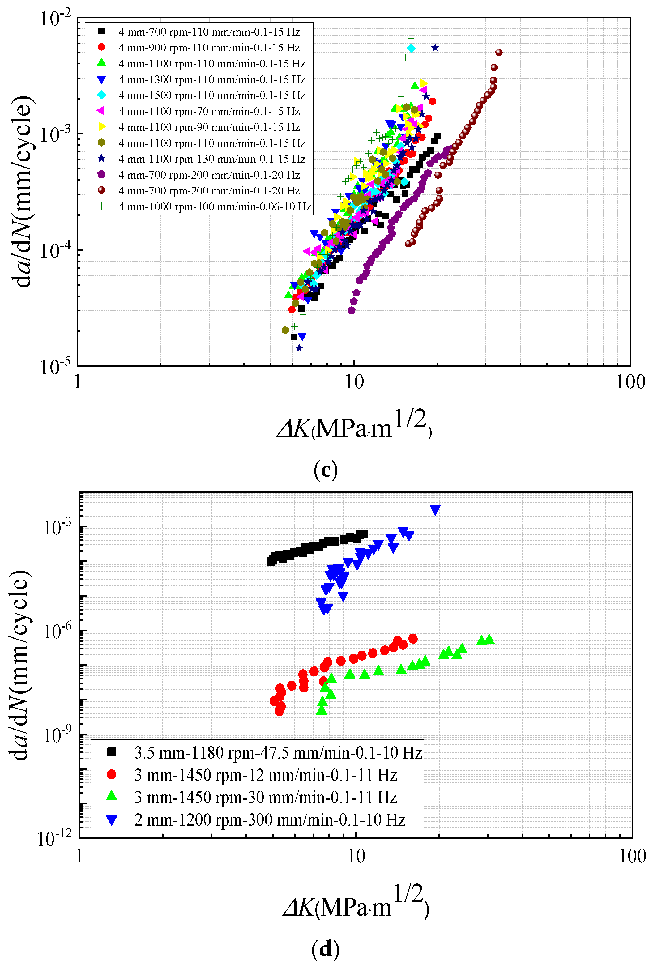
Figure 1. FCGR of 2024-T3 FSWed joints: (a) base material; (b) thickness from 8 mm to 5 mm of FSWed joints; (c) thickness of 4 mm of FSWed joints; (d) thickness from 3.5 mm to 2 mm of FSWed joints.

Moreover, loading frequency demonstrates a significant effect on the FCGR. Within the examined stress ratio range, an increase in loading frequency results in a corresponding rise in the FCGR. This behavior is associated with reduced crack closure effects, which become more pronounced at higher frequencies. Additionally, under otherwise identical conditions, the FCGR increases as the stress ratio rises, which is consistent with the well-known effect of reduced crack closure and increased effective stress intensity range at higher stress ratios.

Figure 1b–d present the FCGR data under different welding process parameters. The results indicate that, within the range of data selected for this article, increasing the rotational speed and welding speed of the tool leads to higher crack growth rates in the welded specimens. This is likely due to the elevated heat input and altered microstructural characteristics—such as grain refinement, residual stress distribution, and phase evolution—influenced by more intense thermo-mechanical effects during the welding process. These changes may weaken the crack resistance in the stir zone or the thermal–mechanical affected zone, thereby accelerating fatigue crack propagation. Overall, these findings highlight the complex interplay between geometrical, mechanical, and process parameters in determining the fatigue performance of FSWed joints.

To further demonstrate the relationship between input parameters and the FCGR, we calculated the Kendall correlation values between the input variables and the FCGR for both the BM and FSM, as shown in Table 3 and Table 4. The p-values for these correlations are all extremely small (ranging from 1.34 × 10⁻¹⁴ to 1.49 × 10⁻⁵), indicating statistically significant correlations. For example, the negative correlation between thickness and the FCGR suggests that as the thickness of the base material increases, the fatigue crack growth rate decreases, which is consistent with our understanding of the mechanical behavior of materials under cyclic loading. Similarly, the positive correlation between loading frequency and the FCGR implies that higher loading frequencies lead to increased fatigue crack growth rates, which is also in line with well-known fatigue theories.

Table 3. The Kendall correlation value of the input variables and the FCGR for BM.

	Thickness	Loading Frequency	Stress Ratio	Stress Intensity Factor
Values	−0.2336	0.1607	−0.1266	0.1207
p	1.34 × 10−14	1.10 × 10−6	5.35 × 10−5	1.49 × 10−5

Table 4. The Kendall correlation value of the input variables and the FCGR for FSM.

	Thickness	Rotational Speed	Welding Speed	Loading Frequency	Stress Ratio	Stress Intensity Factor
Values	−0.1144	−0.0372	0.3752	0.4333	−0.3497	0.3936
p	1.17 × 10−6	9.41 × 10−2	6.69 × 10−63	9.12 × 10−72	2.12 × 10−42	3.45 × 10−77

Although ΔK exhibits a strong correlation with the fatigue crack growth rate, the Kendall correlation analysis indicates that welding speed, loading frequency, and stress ratio also show statistically significant correlations with the FCGR. This demonstrates that the variation in da/dN cannot be explained by ΔK alone, and that welding and loading parameters contribute additional, non-negligible information to the prediction task. The improved predictive accuracy achieved by the multi-parameter ML models further confirms that these factors play an active role beyond the classical ΔK-driven framework.

3. Machine Learning Algorithms

3.1. Deep Back-Propagation (Deep BP) Network

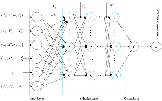
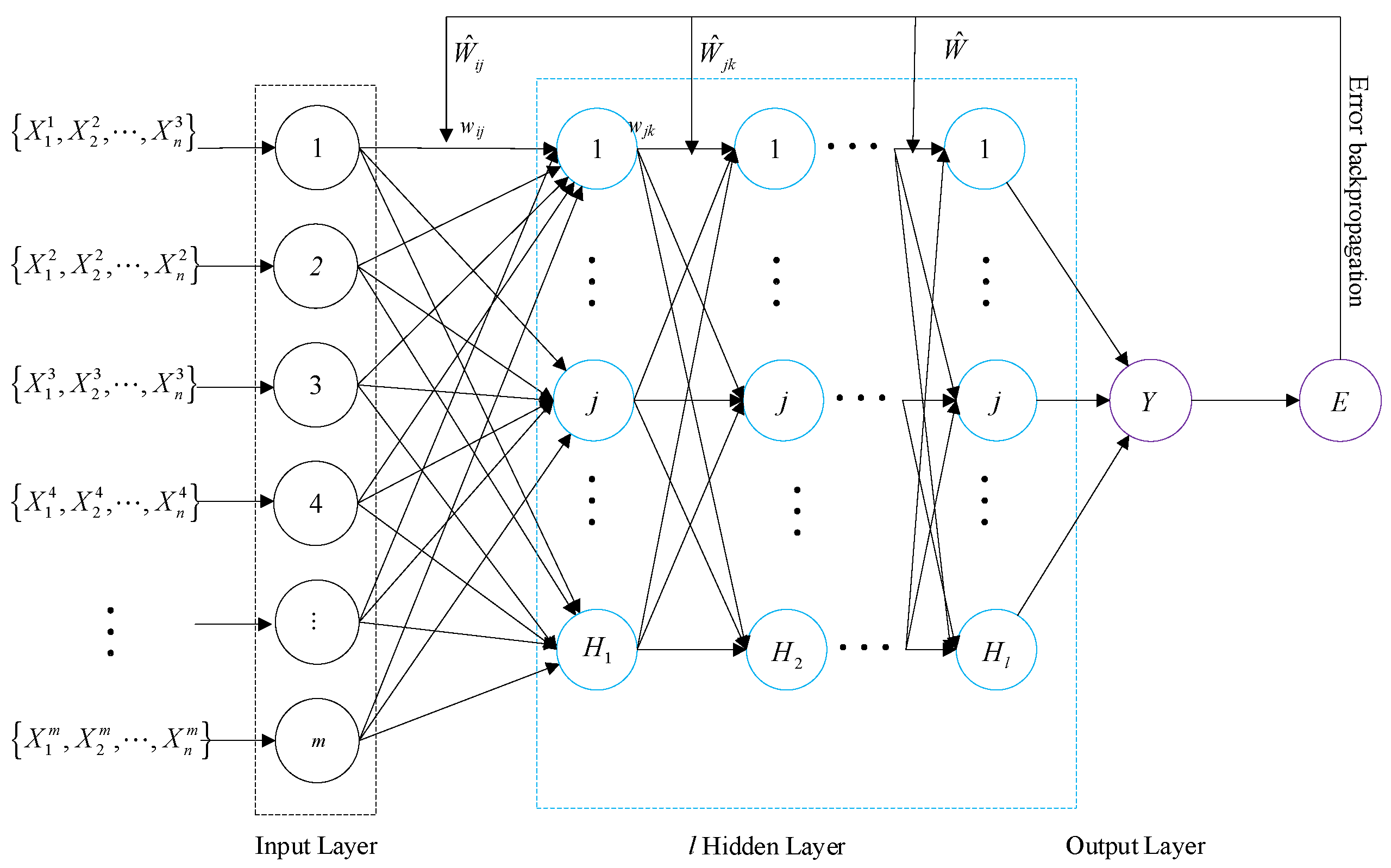
Deep BP networks extend traditional BP architectures by stacking multiple hidden layers (>3 layers) to achieve hierarchical feature learning [41]. Rooted in multi-layer feed-forward neural networks (FFNNs), they leverage iterative forward/backward passes to minimize prediction errors. The structure of the Deep BP network is shown in Figure 2, where $\left\{X_1^j,X_2^j,\dots ,X_n^j\right\}$ is the input for the j-th input feature and $\left\{Y_1,Y_2,\dots ,Y_n\right\}$ is the output.

Figure 2. Structure of Deep BP network. (Black circle: input neurons; Blue circle: hidden neurons; Purple circle: outputs or errors in the online color version).

Below are the key mechanisms and core formulas:

In forward propagation, for neuron j in layer l, the output is calculated as follows:

$$ne{t}_j^l=\sum w_{ij}^l·f\left(ne{t}_j^{l-1}\right)+b_j^l$$

(1)

where $f\left(\cdot \right)$ indicates nonlinear activation, $w_{ij}^l$ is weight and connects layer l to l + 1, and $b_j^l$ denotes the thresholds for neuron j in layer l.

In error back-propagation, the output error propagates backward. Gradient computation uses the chain rule.

For the output layer:

$${\delta }_k^{out}=(T_k-Y_k)\cdot f^{\prime }(ne{t}_k)$$

(2)

where $T_k$ is true value and $Y_k$ is forecasting value.

For the hidden layer:

$${\delta }_j^l=f^{\prime }(ne{t}_k)\cdot {\displaystyle \sum _k{\delta }_k^{l+1}}\cdot w_{jk}^{l+1}$$

(3)

For the weight update:

$$\begin{array}{l}{\widehat{W}}_{ij}^l\leftarrow w_{ij}^l-\eta \partial E/\partial w_{ji}^l\\ E={\displaystyle \frac{1}{2}}{\displaystyle \sum {\left(T-Y\right)}^2}\end{array}$$

(4)

where $\eta$ is learning rate and E is the mean square error (MSE).

3.2. Random Forest (RF)

Random Forest (RF) regression, introduced by Breiman [42,43], is an ensemble learning method that constructs multiple decision trees during training and outputs the mean prediction of individual trees. It addresses overfitting in traditional regression trees while maintaining high accuracy with high-dimensional data and small samples.

The process of RF for forecasting fatigue crack growth rate is summarized below [44].

Given n observations: $T{r}_n={\left\{\left({\mathit{X}}_i,Y_i\right)\right\}}_{i=1}^n$, where ${\mathit{X}}_i\in R^m$ are input features (e.g., stress intensity factor) and $Y_i\in R$ denotes the true fatigue crack growth rate. The RF method first draws N_tr bootstrap samples of size n with replacement. For each bootstrap replicate, an un-pruned regression tree is grown. At each node, the split that minimizes the MSE is selected after examining only a random subset of mtry predictors. Then, splitting continues recursively until the number of observations in a leaf falls below a user-defined minimum. Finally, the N_tr trees are aggregated by averaging their predictions to yield the final RF predictor.

3.3. Support Vector Regression (SVR)

Support Vector Regression (SVR) is a kernel-based regression technique derived from Support Vector Machines (SVMs) [45]. It optimizes a regression hyperplane while tolerating ε-insensitive errors. Its primal convex optimization problem is formalized as follows:

$$\begin{array}{l}\underset{w,b,\xi ,{\xi }^{\ast }}{\min }{\displaystyle \frac{1}{2}}\parallel w{\parallel }^2+C{\displaystyle \sum _n^{i=1}}({\xi }_i+{\xi }_i^{\ast })\\ \mathrm{s}.\mathrm{t}.\hspace{1em}\left\{\begin{array}{c}{Y}_i-f({\mathit{X}}_i)\le \epsilon +{\xi }_i\\ f({\mathit{X}}_i)-Y\le \epsilon +{\xi }_i^{\ast }\\ {\xi }_i,{\xi }_i^{\ast }\ge 0\end{array}\right.\end{array}$$

(5)

where ${\xi }_i,{\xi }_i^{\ast }$ are slack variables accommodating outliers, $C$ is a regularization parameter penalizing large errors, and $\epsilon$ denotes margin width determining prediction tolerance.

The dual solution yields predictions dependent on sparse support vectors:

$$\widehat{Y}=\sum _{i\in SV}({\alpha }_i-{\alpha }_i^{\ast })K\left(X_i,X\right)+b$$

(6)

where ${\alpha }_i$ and ${\alpha }_i^{\ast }$ are Lagrangian multipliers and $K\left(\cdot \right)$ is a kernel function. Common choices include the Gauss kernel function, Radial Basis Function (RBF), Linear kernel, and Polynomial function.

3.4. K-Nearest Neighbors (KNN)

K-Nearest Neighbors (KNN) regression is a non-parametric machine learning method for regression analysis [46]. Unlike parametric models, KNN requires no a priori assumptions about data distributions. For a new data point, it identifies the k closest training samples in feature space using distance metrics. The predicted output is computed as the unweighted mean of the targets of these neighbors. This architecture enables KNN to model complex nonlinear relationships between features and target variables through local approximations. The model’s behavior critically depends on the parameter k. A small k value generates high-variance predictions that may amplify high-frequency fluctuations (e.g., measurement noise), increasing overfitting risk. A large k value produces over-smoothed outputs that potentially ignore localized trends, leading to underfitting. In practice, the choice of distance metric (e.g., Euclidean, Manhattan, Mahalanobis, or learned metrics) and neighbor weighting (uniform vs. distance-weighted) are additional hyper-parameters. When dimensionality grows, distances become less informative—a phenomenon known as the curse of dimensionality—often necessitating dimensionality reduction or metric learning to retain predictive power.

3.5. Establishment of the ML Models

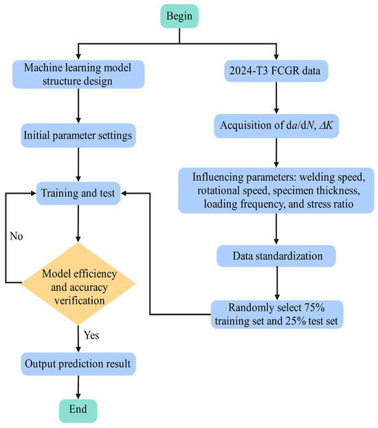
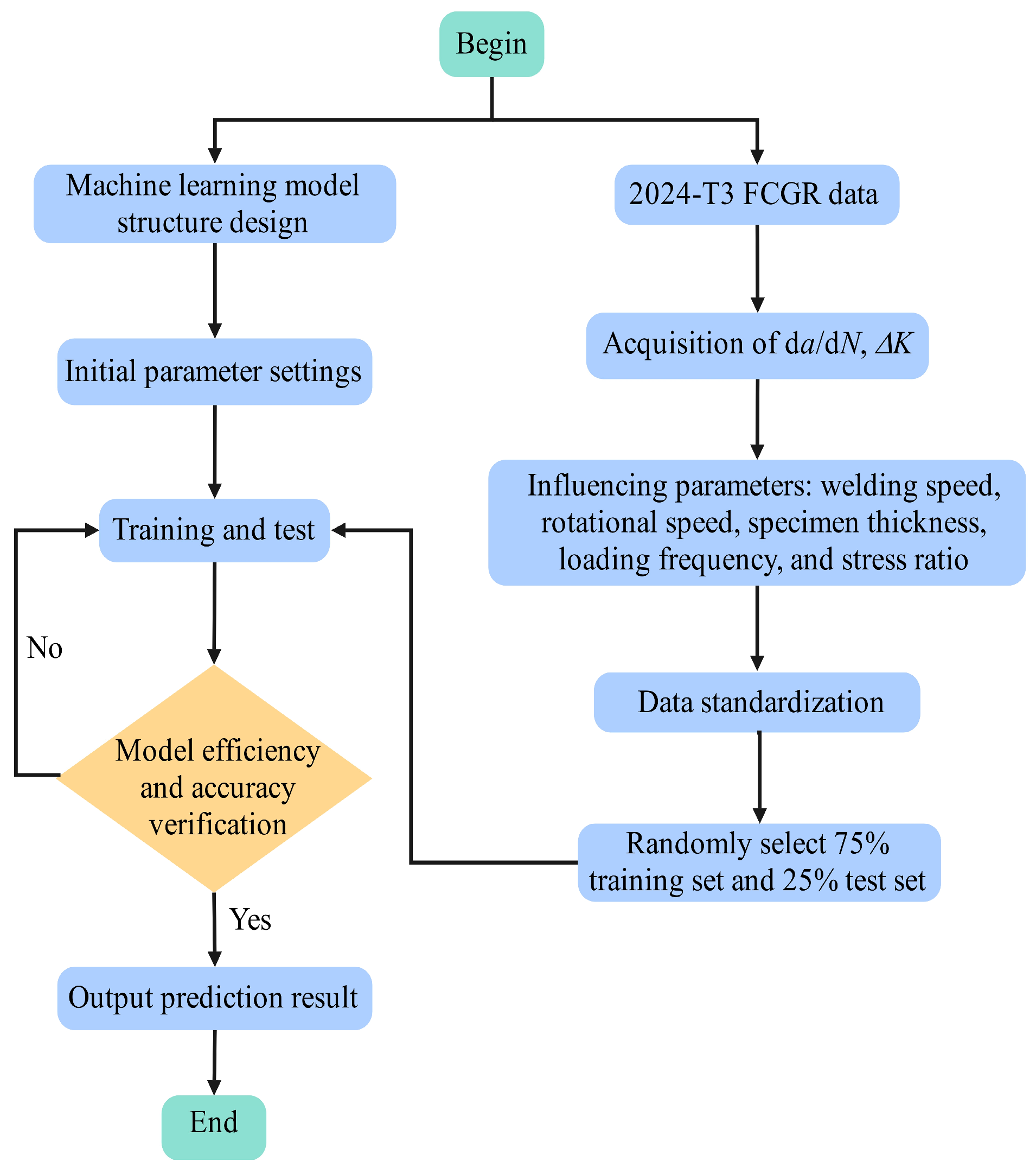
The flowchart for the establishment of the machine learning (ML) models is illustrated in Figure 3. First, experimental data on the fatigue crack growth rate (da/dN) of 2024 aluminum alloy were collected under varying welding speeds, rotational speeds, specimen thicknesses, loading frequencies, and stress ratios. The dataset comprises six input features, which include the stress intensity factor range (ΔK) and five influencing parameters, in addition to one output variable, the fatigue crack growth rate (da/dN). To eliminate the effects of differing data scales and improve training stability, all input features were standardized. Next, 75% of the dataset was randomly selected as the training set, while the remaining 25% was used as the test set to evaluate model performance. The data were then input into the initialized machine learning models for training. After training, the models were validated to assess their prediction accuracy and computational efficiency. The evaluation metrics used included the coefficient of determination (R²), mean square error (MSE), root mean square error (RMSE), mean absolute error (MAE), and mean absolute percentage error (MAPE). Higher R² and lower MSE, RMSE, MAE, and MAPE values indicate acceptable prediction results. Additionally, training time (t) was used as a measure of computational efficiency [44]. Finally, the optimized training results were output for analysis and comparison.

Figure 3. Flowchart of machine learning model.

It should be noted that the stress intensity factor range (ΔK) is a dominant driving force for fatigue crack growth from a fracture mechanics perspective. However, the objective of this study is not to replace or rediscover the classical ΔK–da/dN relationship, but to investigate how welding parameters and loading conditions modulate fatigue crack growth behavior under a given ΔK level.

To avoid the machine learning models being trivially dominated by ΔK, ΔK is treated as a shared baseline variable, while welding speed, rotational speed, specimen thickness, loading frequency, and stress ratio are incorporated as additional explanatory features. In this way, the models are trained to learn the residual variation in da/dN associated with process-induced residual stresses, geometric constraints, and loading effects beyond the primary ΔK dependence. This strategy enables the ML models to capture the coupled and nonlinear influence of welding and loading parameters without violating fracture mechanics principles.

The parameters of each ML model are determined primarily on the basis of the literature [41,44,45,46,47] and through multiple experimental tests.

For Deep BP, a three-hidden-layer architecture is used, with the number of neurons in each layer determined via grid search, and the model is trained using the Levenberg–Marquardt algorithm (trainlm) [41,45].

For RF, N_tr is set as 50, and mtry is set to approximately m/3, where m is the dimensionality of the input vector, as recommended in [44].

For SVR, the Gauss kernel function is used to capture complex nonlinear relationships. The mathematical expression of the Gauss kernel function is $K\left(X_i,X\right)=\exp \left(-{‖X_i-X‖}^2/2{\sigma }^2\right)$. The hyperparameters $\sigma$ (kernel scale), $\epsilon$ (insensitivity margin), and C (regularization) are optimized through a grid search over the following ranges: $\sigma \in \left[0.1, 10\right]$, $\epsilon \in \left[0.01, 0.5\right]$, and $C\in \left[{10}^{-3}, {10}^3\right]$ [45,47].

For KNN, the value k = 5 was chosen because five-fold cross-validation [46] showed it produced the smallest prediction error among k = 1, 3, 5, 7, and 9, and uniform weighting was used to avoid over-emphasizing noisy neighbors.

4. Results and Discussion

For the base material, the input parameters include specimen thickness, loading frequency, stress ratio, and ΔK, totaling 576 data points. Of these, 75% (432 data points) were used as the training set for ML models, while the remaining 25% (144 data points) were reserved as the testing set to evaluate model prediction accuracy. For the FSWed joints, the input parameters include welding speed, rotational speed, specimen thickness, loading frequency, stress ratio, and ΔK, for a total of 996 data points. Similarly, 75% (747 data points) were used as the training set for ML models, while the remaining 25% (249 data points) were reserved as the testing set for model evaluation. Four machine learning models were used to predict the fatigue crack growth rate of the 2024-T3 base material and FSWed joints. The accuracy and efficiency of the prediction results of the four ML models were compared to demonstrate their respective advantages and disadvantages. The prediction results of the ML models listed in this paper are the best results obtained after multiple experiments.

4.1. Base Material Prediction

Table 5 summarizes the predictive accuracy and computational efficiency of four ML models for estimating the FCGR of the 2024-T3 base material. For the training set, the Deep BP, RF, and KNN models all achieve R² values above 0.98, indicating excellent fitting capabilities. Among them, the Deep BP model exhibits the highest overall accuracy, with R² = 0.9946, MAE = 0.0940, MAPE = 0.0277, MSE = 0.0231, and RMSE = 0.1519, which ranks first across all five evaluation metrics. This reflects its strong predictive performance on the training data. The performance of the KNN model is also comparable, with only a small margin between that of the Deep BP model, suggesting similar learning capacity when sufficient training data are available. Meanwhile, for the testing set, the Deep BP model continues to outperform the other models across all five evaluation indicators, confirming its superior generalization ability and robustness. These results indicate that Deep BP provides the most reliable and accurate predictions for the FCGR of the 2024-T3 base material among the four models evaluated.

Table 5. Evaluation metrics of base material machine learning models.

Model	Training Set					Testing Set					t (s)
	MAE (mm cycle−1)	MAPE	MSE (mm cycle−1)	RMSE (m cycle−1)	R2	MAE (mm cycle−1)	MAPE	MSE (mm cycle−1)	RMSE (mm cycle−1)	R2
Deep BP	0.0940	0.0277	0.0231	0.1519	0.9946	0.0959	0.322	0.0224	0.1498	0.9952	3.9715
RF	0.1655	0.1298	0.0738	0.2717	0.9833	0.2023	0.0971	0.0903	0.3004	0.9789	0.8762
SVR	0.2347	0.0790	0.2799	0.5291	0.9361	0.1677	0.0634	0.1342	0.3663	0.9696	0.7159
KNN	0.0941	0.0302	0.0387	0.1967	0.9912	0.1785	0.0624	0.0767	0.2770	0.9824	0.2303

The KNN model exhibited the shortest training time, requiring only 0.2303 s, highlighting its computational efficiency. The RF and SVR models followed, with training times of 0.8762 s and 0.7159 s, respectively, ranking second and third in efficiency. In contrast, the Deep BP model had the longest training time, reaching 3.9715 s, which is approximately 17 times longer than that of the KNN model. However, relative to finite element modeling analysis, the computational efficiency of all four ML models is markedly improved.

Table 6 presents the comprehensive rankings of all four ML models based on their performance across multiple evaluation metrics in both training and testing periods. Higher scores for error metrics (MAE, MAPE, MSE, and RMSE), R², and lower computation time (t) indicate better performance. Higher scores indicate better performance in the ranking-based evaluation scheme adopted in this study.

Table 6. Ranking of base material prediction models.

Model	Training Set					Testing Set					t (s)	Total Ranking Score	Rank
	MAE (mm cycle−1)	MAPE	MSE (mm cycle−1)	RMSE (mm cycle−1)	R2	MAE (mm cycle−1)	MAPE	MSE (mm cycle−1)	RMSE (mm cycle−1)	R2
Deep BP	4	4	4	4	4	4	4	4	4	4	1	41	1
RF	2	1	2	2	2	1	1	2	2	2	2	19	3
SVR	1	2	1	1	1	3	3	1	1	1	3	18	4
KNN	3	3	3	3	3	2	2	3	3	3	4	32	2

The Deep BP model achieved the highest total score of 41, highlighting its superior overall performance and strong capability in capturing the complex nonlinear relationships inherent in FCGR prediction. It suggests that Deep BP is particularly well suited for tasks involving multivariate interactions and large datasets, where deeper model architectures can effectively learn intricate patterns in the data. Closely following is the KNN model, with a score of 32, indicating a comparable level of predictive performance. The KNN model performed particularly well on the training set, benefiting from its simplicity and non-parametric nature. When the local data distribution is dense and representative, KNN is capable of delivering high accuracy without requiring extensive model tuning. However, its performance on the testing set was slightly inferior to Deep BP, likely due to its sensitivity to data sparsity and inability to generalize well in regions lacking sufficient neighboring samples.

Among the remaining models, the RF model ranked third with a score of 19. While RF demonstrated moderate predictive accuracy, especially in handling nonlinearity and noisy data, it showed larger deviations and slightly weaker generalization compared to the top two models. This may be due to overfitting tendencies or limitations in capturing subtle patterns when the number of decision trees is not sufficiently optimized. The SVR model received the lowest total score of 18, placing it last among the four models evaluated. Despite its theoretical strengths in handling high-dimensional nonlinear regression through kernel functions, SVR underperformed in this study, particularly in terms of accuracy and consistency. Its sensitivity to parameter selection and the relatively small size of the training dataset may have constrained its predictive capacity.

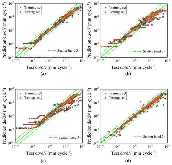
Figure 4 compares the experimentally measured FCGR of the 2024 base material with the predicted results from the four machine learning models, offering a clear visualization of their predictive capabilities. In Figure 4a, the predictions fall entirely within the ±3 times error dispersion band, with most data points densely distributed along the zero-error line, indicating excellent agreement between predicted and experimental values. By contrast, Figure 4b,c show that the RF and SVR models exhibit more pronounced scatter in their predictions. This is particularly evident when the FCGR is less than 1 × 10⁻⁸, where deviations from the experimental data become more significant, suggesting limited predictive stability in this low-growth-rate region. In comparison, Figure 4d demonstrates that the KNN model yields predictions that are largely confined within the ±3 times error band, with many points closely tracking the zero-error line. This reflects the KNN model’s strong predictive consistency and its ability to accurately capture FCGR behavior across the evaluated range.

Figure 4. Comparison of base material test results with prediction data (input variables: ΔK, specimen thickness, loading frequency, and stress ratio; output variable: da/dN): (a) Deep BP; (b) RF; (c) SVR; (d) KNN.

4.2. FSWed Joints Prediction

Table 7 summarizes the predictive accuracy and computational efficiency of four ML models for estimating the FCGR of the 2024-T3 FSWed joints under the influence of five key parameters. For the training set, the R² for both the Deep BP and KNN models exceeds 0.98, indicating excellent fitting performance. Among them, the KNN model achieves the highest overall accuracy, with R² = 0.9848, MAE = 0.0989, MAPE = 0.0253, MSE = 0.0398, and RMSE = 0.1996. It ranks first in terms of R², MAE, and MAPE, and second in MSE and RMSE, demonstrating a strong predictive capability on the training data. The performance gap between the KNN and Deep BP models on the training set is relatively small, suggesting comparable learning capacity under sufficient data coverage. However, for the testing set, the Deep BP model outperforms the other models across all five evaluation metrics, highlighting its superior generalization ability and robustness when applied to unseen data. This indicates that while KNN excels in fitting the training data, Deep BP maintains better performance in scenarios requiring accurate extrapolation or prediction beyond the training domain.

Table 7. Evaluation metrics of FSW machine learning models.

Model	Training Set					Testing Set					t (s)
	MAE (mm cycle−1)	MAPE	MSE (mm cycle−1)	RMSE (mm cycle−1)	R2	MAE (mm cycle−1)	MAPE	MSE (mm cycle−1)	RMSE (mm cycle−1)	R2
Deep BP	0.1277	0.0269	0.0395	0.1987	0.9846	0.1281	0.0283	0.0394	0.1984	0.9845	4.6365
RF	0.2137	0.0486	0.1021	0.3196	0.9606	0.2237	0.0506	0.1035	0.3217	0.9577	0.2067
SVR	0.2973	0.0650	0.2436	0.4936	0.9046	0.2842	0.0656	0.2002	0.4474	0.9217	0.8597
KNN	0.0989	0.0253	0.0398	0.1996	0.9848	0.1755	0.0399	0.0695	0.2636	0.9708	0.1530

The KNN model exhibited the shortest training time, requiring only 0.1530 s, highlighting its computational efficiency. The RF and SVR models followed, with training times of 0.2067 s and 0.8597 s, respectively, ranking second and third in efficiency. In contrast, the Deep BP model had the longest training time, reaching 4.6365 s, which is approximately 30 times longer than that of the KNN model.

This significant difference in training time suggests that, when handling large-scale datasets or real-time applications, the KNN model offers a clear advantage in terms of computational efficiency. Although Deep BP achieves the highest accuracy, its substantially longer training time may limit its practicality in scenarios where rapid model deployment or frequent retraining is required. Therefore, in applications prioritizing speed and low computational cost, the KNN model may demonstrate superior performance efficiency compared to Deep BP, particularly as the dataset size increases.

In Table 8, the Deep BP model achieved the highest total score of 38, highlighting its superior overall performance and strong capability in capturing the complex nonlinear relationships inherent in FCGR prediction of FSWed joints. Closely following is the KNN model, with a score of 37, indicating a comparable level of predictive performance. The KNN model performed particularly well in terms of accuracy and simplicity, with minimal parameter tuning required and strong performance in data regions with good local coverage. Among the remaining models, the RF model ranked third, with a total score of 23. While RF demonstrated decent generalization ability and resilience to overfitting, especially on small-to-medium datasets, its performance was limited by relatively higher prediction errors and lower consistency in low FCGR regions. The SVR model received the lowest score of 12, ranking last among the four models. Although SVR is theoretically well suited for handling nonlinear problems through kernel functions, its performance in this study was hindered by lower prediction accuracy and greater deviation from experimental data, particularly in regions with small crack growth rates. This may be attributed to limited training samples or sensitivity to parameter selection in high-dimensional feature spaces.

Table 8. Ranking of FSW prediction models.

Model	Training Set					Testing Set					t (s)	Total Ranking Score	Rank
	MAE (mm cycle−1)	MAPE	MSE (mm cycle−1)	RMSE (mm cycle−1)	R2	MAE (mm cycle−1)	MAPE	MSE (mm cycle−1)	RMSE (mm cycle−1)	R2
Deep BP	3	3	4	4	3	4	4	4	4	4	1	38	1
RF	2	2	2	2	2	2	2	2	2	2	3	23	3
SVR	1	1	1	1	1	1	1	1	1	1	2	12	4
KNN	4	4	3	3	4	3	3	3	3	3	4	37	2

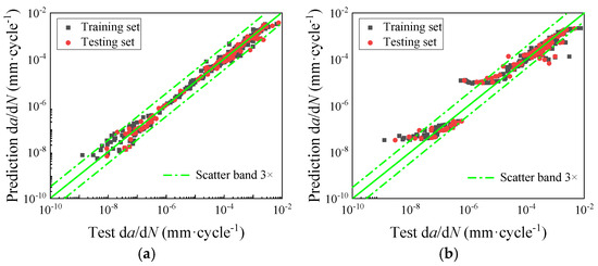
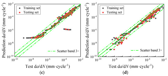
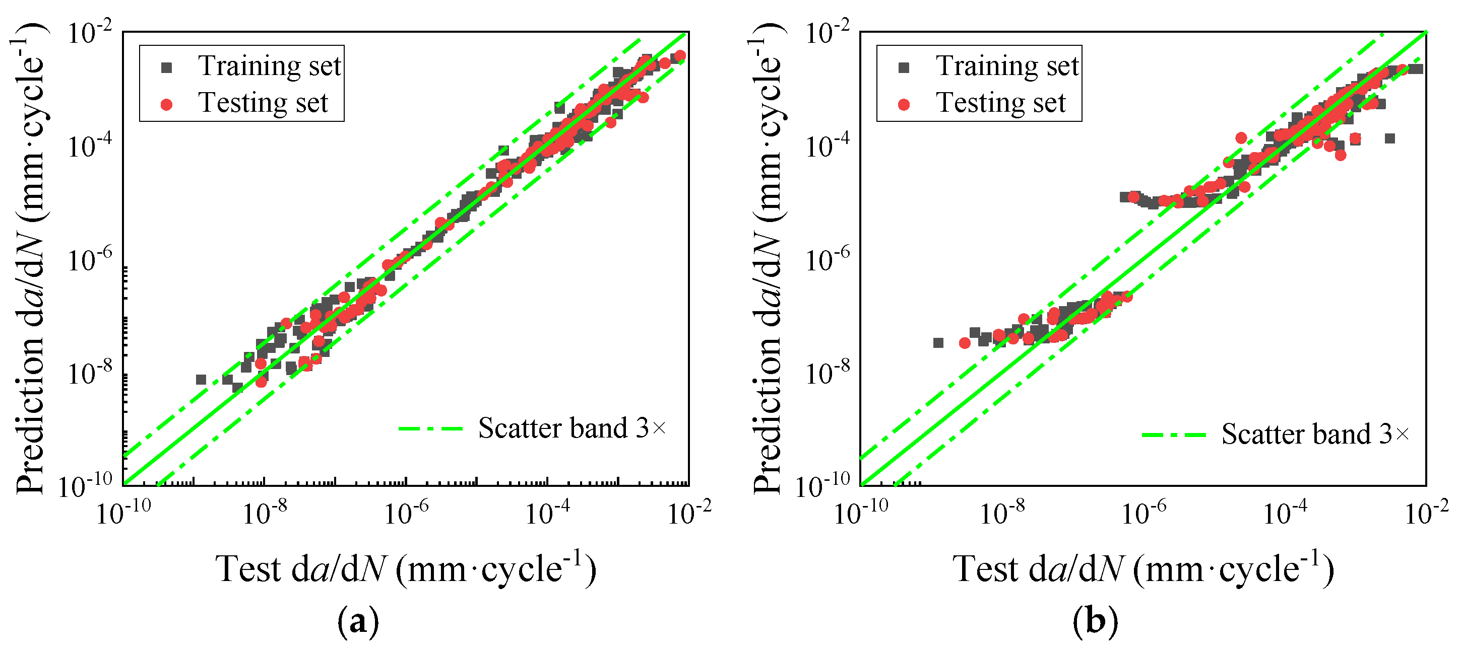
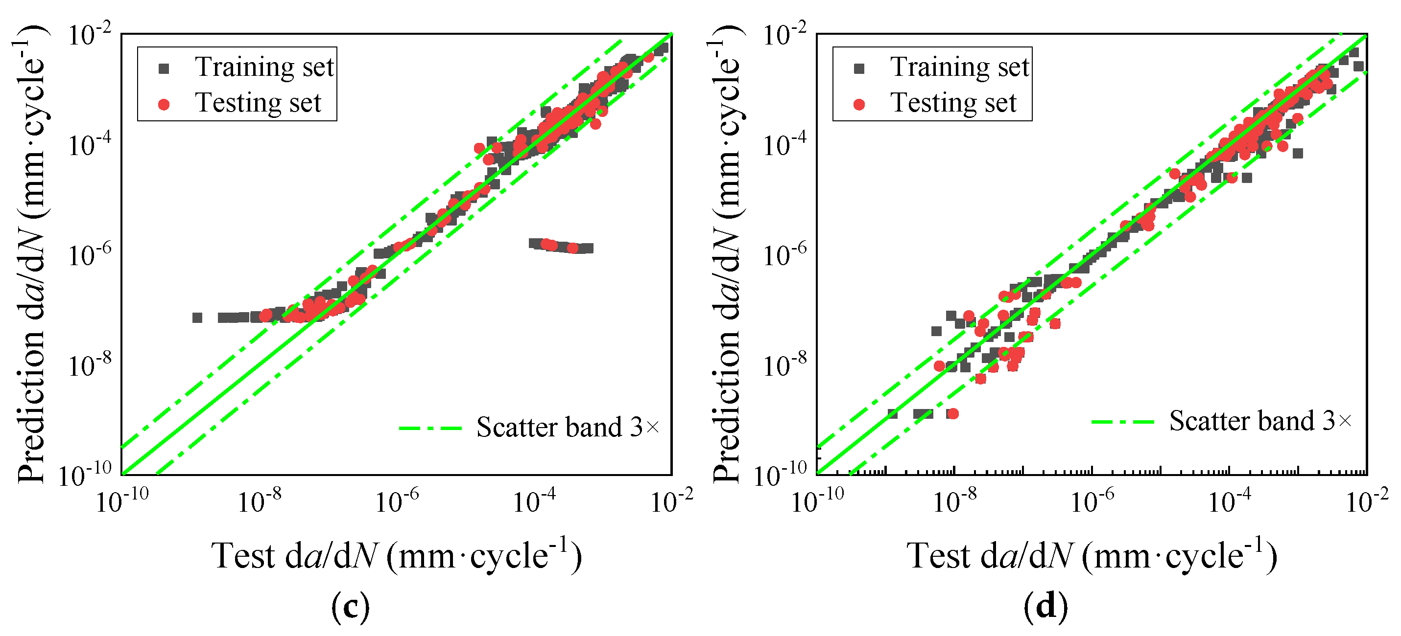
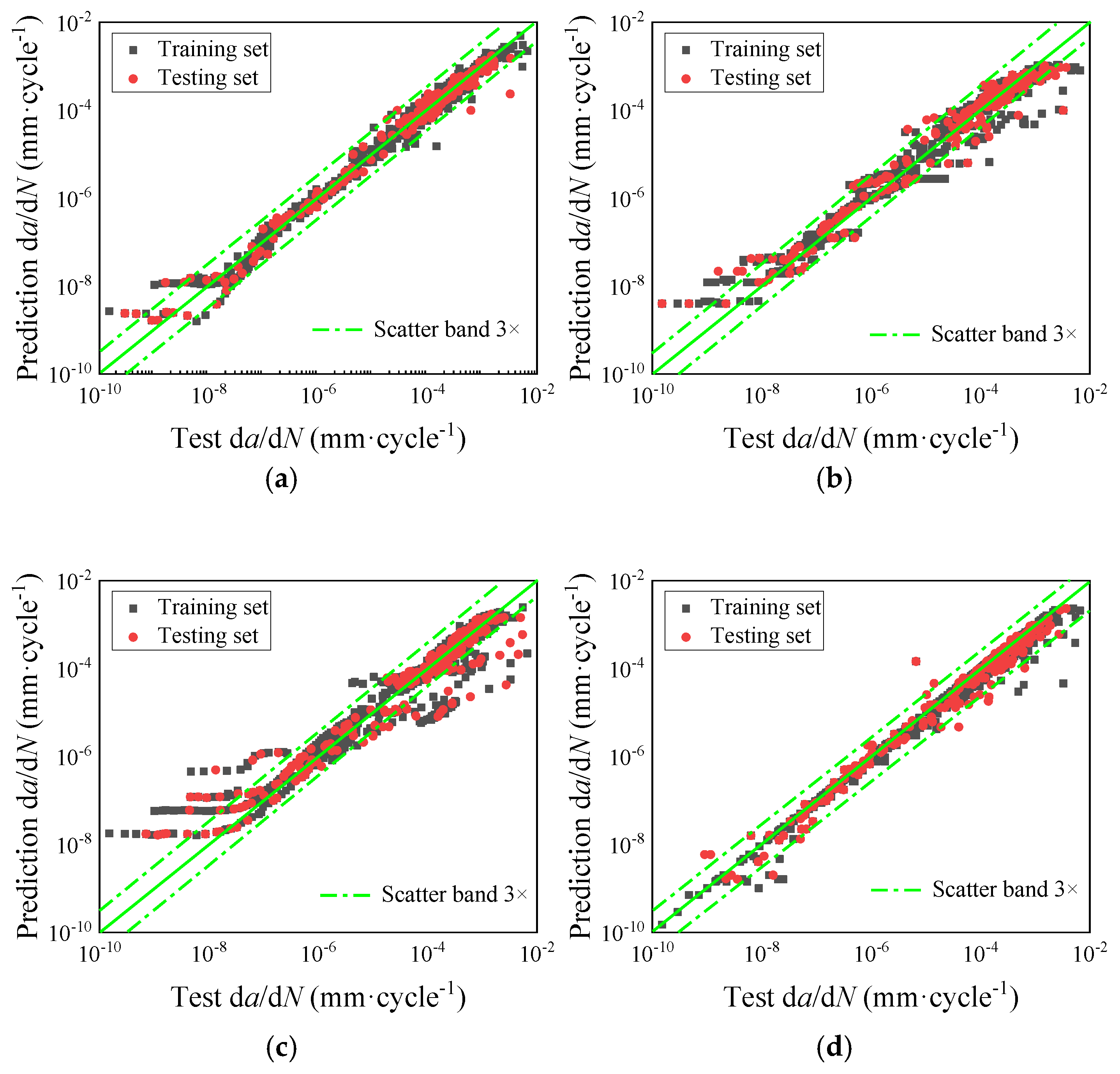
Figure 5 presents a comparison between the experimental FCGR data of the 2024-T3 FSWed joints and the predicted results obtained from the four ML models, effectively illustrating their predictive performance. As shown in Figure 5a, when the FCGR is below 1 × 10⁻⁸, noticeable deviations occur between the predicted and experimental results. However, as the FCGR exceeds 1 × 10⁻⁸, most predictions fall within the ±3 times error dispersion band, indicating improved model reliability in this range. Figure 5b,c reveal that the prediction results of the RF and SVR models exhibit greater dispersion, particularly when the FCGR is below 1 × 10⁻⁸, where the deviation from the experimental data becomes more pronounced. In contrast, Figure 5d shows that the predictions from the KNN model are largely concentrated within the ±3 times error band, with many data points closely aligned along the zero-error line, reflecting strong predictive accuracy and consistency.

Figure 5. Comparison of test results with prediction data (input variables: ΔK, welding speed, rotational speed, specimen thickness, loading frequency, and stress ratio; output variable: da/dN): (a) Deep BP; (b) RF; (c) SVR; (d) KNN.

5. Conclusions

This study confirms that data-driven approaches provide a viable alternative to classical empirical crack growth formulations when dealing with multi-parameter welding conditions. Machine learning enables direct mapping from processes and loading variables to fatigue crack growth response, avoiding restrictive assumptions on stress ratio dependence, crack closure behavior, or microstructural uniformity. Traditional phenomenological crack growth models, such as the Paris and Forman equations, typically involve two-or three-parameter fitting under specified stress ratios and load interaction assumptions, and often require separate calibration when welding conditions, microstructures, or residual stress states vary. In contrast, the ML models used in this study directly incorporate multiple influencing variables (ΔK, welding speed, rotational speed, specimen thickness, loading frequency, and stress ratio) without requiring explicit constitutive assumptions. This enables the models to capture nonlinear coupling among process parameters, thermal–mechanical effects, and loading conditions. Moreover, the ML predictions were evaluated using quantitative metrics (R², RMSE, MAE, and MAPE), which showed consistently higher accuracy than traditional curve-fitting methods when multi-factor dependencies are considered. Therefore, although a ±3 times error band was used for visual comparison, the statistical indicators confirm that the ML models provide more robust generalization and broader applicability than phenomenological laws, particularly for welded joints with strong process-dependent variability. In addition, the ML approach is not restricted to fixed stress ratios and can be readily updated when new experimental data become available, which offers adaptability not achievable using deterministic empirical crack growth equations. Future work may include hybrid ML mechanism models or physics-informed neural networks to further reduce scatter and improve interpretability.

The main conclusions are as follows:

(1) For the base material, the Deep BP model achieved the best evaluation indicators, with an R2 of 0.9952 on the testing set, highlighting its superior overall performance and strong capability in capturing the complex nonlinear relationships inherent in FCGR prediction. The performance of the KNN model is also comparable, suggesting similar learning capacity when sufficient training data are available. The KNN model exhibited the shortest training time within 0.3 s.

(2) For the FSWed joints, the performance gap between the KNN and Deep BP models on the training set is relatively small, Deep BP slightly outperforms KNN on the test set, suggesting comparable learning capacity under sufficient data coverage. In applications prioritizing speed and low computational cost, the KNN model may demonstrate superior performance efficiency compared to Deep BP, particularly as the dataset size increases. Although Deep BP models require more time, they still take less than 5 s, which offers a significant advantage over finite element analysis and has substantial engineering application value.

(3) The Deep BP and KNN models reflect strong predictive consistency and have the ability to accurately capture FCGR behavior across the evaluated range (1 × 10⁻¹⁰ to 0.01). The prediction results of the RF and SVR models exhibit greater dispersion, particularly when the FCGR is below 1 × 10⁻⁸, where the deviation from the experimental data becomes more pronounced.

Overall, the proposed ML-based framework provides an efficient, flexible, and accurate tool for fatigue crack growth prediction in FSWed joints, with strong potential for integration into aircraft structural integrity assessment and fatigue life management workflows. In particular, the framework can support damage-tolerant design, certification-oriented fatigue evaluation, and maintenance planning by enabling rapid assessment of crack growth behavior under varying welding conditions and operational loading scenarios. Its ability to deliver fast and reliable predictions makes it well suited for early stage design screening, parametric studies, and fleet-level structural health management. Future work will focus on validating the proposed framework through dedicated experiments using a new, fully independent dataset to further assess its generalization capability.

References

- Nejad, R.M.; Sina, N.; Moghadam, D.G.; Branco, R.; Macek, W.; Berto, F. Artificial neural network based fatigue life assessment of friction stir welding AA2024-T351 aluminum alloy and multi-objective optimization of welding parameters. Int. J. Fatigue 2022, 160, 106840. [Google Scholar] [CrossRef] [Scilit]
- Yadav, V.K.; Gaur, V.; Singh, I.V. Combined effect of residual and mean stresses on fatigue behavior of welded aluminum 2024 alloy. Int. J. Fatigue 2022, 155, 106565. [Google Scholar] [CrossRef] [Scilit]
- Guo, Y.N.; Ma, Y.E.; Wang, F. Dynamic fracture properties of 2024-T3 and 7075-T6 aluminum friction stir welded joints with different welding parameters. Theor. Appl. Fract. Mec. 2019, 104, 102372. [Google Scholar] [CrossRef] [Scilit]
- Gao, J.X.; Heng, F.; Yuan, Y.; Liu, Y.Y. Fatigue Reliability Analysis of Composite Material Considering the Growth of Effective Stress and Critical Stiffness. Aerospace 2023, 10, 785. [Google Scholar] [CrossRef] [Scilit]
- Li, L.; Li, X.; Zhan, Z.; Hu, W.; Meng, Q. Fatigue Life Prediction for 2060 Aluminium–Lithium Alloy with Impact Damage. Aerospace 2024, 11, 536. [Google Scholar] [CrossRef] [Scilit]
- Zhang, X.S.; Ma, Y.E.; Li, W.Y.; Huang, W.; Zhang, W.H.; Wang, Z.H. A review of residual stress effects on fatigue properties of friction stir welds. Crit. Rev. Solid State 2023, 48, 775–813. [Google Scholar] [CrossRef] [Scilit]
- Xie, X.F.; Jiang, W.; Luo, Y.; Xu, S.; Gong, J.M.; Tu, S.T. A Model to Predict the Relaxation of Weld Residual Stress by Cyclic Load: Experimental and Finite Element Modeling. Int. J. Fatigue 2017, 95, 293–301. [Google Scholar] [CrossRef] [Scilit]
- Lian, Z.H.; Li, M.J.; Lu, W.C. Fatigue life prediction of aluminum alloy via knowledge-based machine learning. Int. J. Fatigue 2022, 157, 106716. [Google Scholar] [CrossRef] [Scilit]
- Zerbst, U.; Ainsworth, R.A.; Beier, H.T.; Pisarski, H.; Zhang, Z.L.; Nikbin, K.; Pagel, T.N.; Münstermann, S.; Kucharczyk, P.; Klingbeil, D. Review on fracture and crack propagation in weldments—A fracture mechanics perspective. Eng. Fract. Mech. 2014, 132, 200–276. [Google Scholar] [CrossRef] [Scilit]
- Guo, Y.N.; Ma, Y.E.; Zhang, X.S.; Qian, X.D.; Li, J. Study on residual stress distribution of 2024-T3 and 7075-T6 aluminum dissimilar friction stir welded joints. Eng. Fail. Anal. 2020, 118, 104911. [Google Scholar] [CrossRef] [Scilit]
- Wang, L.; Qian, X.D. Effects of pre-tension and fatigue loadings on the evolution of welding. Eng. Struct. 2024, 301, 117272. [Google Scholar] [CrossRef] [Scilit]
- Anderson-Wedge, K.; Stubblefield, G.; Zhu, N.; Long, B.; Daniewicz, S.R.; Allison, P.; Sowards, J.; Rodriguez, O.; Amaro, R. Characterization of the evolution of 2219-T87 aluminum as a function of the friction stir welding process. Int. J. Fatigue 2021, 142, 105954. [Google Scholar] [CrossRef] [Scilit]
- Lan, Z.; Zhong, H.L.; Li, S.C.; Zhao, H.; Chen, J.; Qi, L. Microstructure, mechanical properties and fatigue crack growth behavior of friction stir welded joint of 6061-T6 aluminum alloy. Int. J. Fatigue 2020, 135, 105556. [Google Scholar] [CrossRef] [Scilit]
- Wang, L.; Cong, J.H.; Ren, J.G.; Hui, L.; Zhou, S. Effect of Parameters on Fatigue Properties and Crack Propagation Behavior of Friction Stir Crack Repaired Al2024. Metals 2020, 10, 1026. [Google Scholar] [CrossRef] [Scilit]
- Delijaicov, S.; Silva, P.A.O.; Resende, H.B.; Batalha, M.H.F. Effect of weld parameters on residual stress, hardness and microstructure of dissimilar AA2024-T3 and AA7475-T761 friction stir welded joints. Mater. Res. 2018, 21, e20180108. [Google Scholar] [CrossRef] [Scilit]
- Yu, H.D.; Zheng, B.; Lai, X.M. A modeling study of welding stress induced by friction stir welding. J. Mater. Process Technol. 2018, 254, 213–220. [Google Scholar] [CrossRef] [Scilit]
- Saravanakumar, R.; Rajasekaran, T.; Pandey, C.; Menaka, M. Mechanical and Microstructural Characteristics of Underwater Friction Stir WeldedAA5083 Armor-Grade Aluminum Alloy Joints. J. Mater. Eng. Perform. 2022, 31, 8459–8472. [Google Scholar] [CrossRef] [Scilit]
- Saravanakumar, R.; Rajasekaran, T.; Pandey, C.; Menaka, M. Influence of Tool Probe Profiles on the Microstructure and Mechanical Properties of Underwater Friction Stir Welded AA5083 Material. J. Mater. Eng. Perform. 2022, 31, 8433–8450. [Google Scholar] [CrossRef] [Scilit]
- Ma, Y.E.; Staron, P.; Fischer, T.; Irving, P.E. Size effects on residual stress and fatigue crack growth in friction stir welded 2195-T8 aluminium-Part I: Experiments. Int. J. Fatigue 2011, 33, 1417–1425. [Google Scholar] [CrossRef] [Scilit]
- Ma, Y.E.; Staron, P.; Fischer, T.; Irving, P.E. Size effects on residual stress and fatigue crack growth in friction stir welded 2195-T8 aluminium-Part II: Modelling. Int. J. Fatigue 2011, 33, 1426–1434. [Google Scholar] [CrossRef] [Scilit]
- Musuva, J.K.; Radon, J.C. The Effect of Stress Ratio and Frequency on Fatigue Crack Growth. Fatigue Fract. Eng. M. 1979, 1, 457–470. [Google Scholar] [CrossRef] [Scilit]
- Long, X.Y.; Yu, M.C.; Liao, W.W.; Jiang, C. A deep learning-based fatigue crack growth rate measurement method using mobile phones. Int. J. Fatigue 2023, 167, 107327. [Google Scholar] [CrossRef] [Scilit]
- Rathore, S.; Kumar, A.; Kumar, A.; Mishra, K.; Singh, A. Prediction of sub-critical fatigue crack growth rate in a high-carbon tempered martensitic steel at varying R ratio: Experimental investigation and machine learning based modelling. Int. J. Fatigue 2025, 193, 108804. [Google Scholar] [CrossRef] [Scilit]
- Santos, B.; Infante, V.; Barros, T.; Baptista, R. Study of fatigue crack propagation on modified CT specimens under variable amplitude loadings using machine learning. Int. J. Fatigue 2024, 184, 108332. [Google Scholar] [CrossRef] [Scilit]
- Sun, L.; Huang, X.P. Prediction of fatigue crack propagation lives based on machine learning and data-driven approach. J. Ocean Eng. Sci. 2024, 9, 592–604. [Google Scholar] [CrossRef] [Scilit]
- Kamble, R.G.; Raykar, N.R.; Jadhav, D.N. Machine learning approach to predict fatigue crack growth. Mater. Today Proc. 2021, 38, 2506–2511. [Google Scholar] [CrossRef] [Scilit]
- Wang, H.X.; Zhang, W.F.; Sun, F.Q.; Zhang, W. A Comparison Study of Machine Learning Based Algorithms for Fatigue Crack Growth Calculation. Materials 2017, 10, 543. [Google Scholar] [CrossRef] [Scilit] [PubMed]
- Fang, X.; Liu, G.J.; Wang, H.H.; Xie, Y.C.; Tian, X.J.; Leng, D.X.; Mu, W.L.; Ma, P.L.; Li, G.B. Fatigue crack growth prediction method based on machine learning model correction. Ocean Eng. 2022, 266, 112996. [Google Scholar] [CrossRef] [Scilit]
- Guo, Y.N.; Li, P.Y. Effect of Residual Stress and Microstructure on the Fatigue Crack Growth Behavior of Aluminum Friction Stir Welded Joints. Materials 2024, 17, 385. [Google Scholar] [CrossRef] [Scilit] [PubMed]
- Moghadam, D.G.; Farhangoost, K. Influence of welding parameters on fracture toughness and fatigue crack growth rate in friction stir welded nugget of 2024-T351 aluminum alloy joints. Trans. Nonferrous Met. Soc. China 2016, 26, 2567–2585. [Google Scholar] [CrossRef] [Scilit]
- Moreira, P.M.G.P.; Castro, P.M.S.T.D. Fatigue crack growth on FSW AA2024-T3 aluminum joints. Key Eng. Mater. 2012, 498, 126–138. [Google Scholar]
- Wang, L.; Hui, L.; Zhou, S.; Xu, L.; He, B. Effect of corrosive environment on fatigue property and crack propagation behavior of Al 2024 friction stir weld. Trans. Nonferrous Met. Soc. China 2016, 26, 2830–2837. [Google Scholar] [CrossRef] [Scilit]
- Wang, W.; Qiao, K.; Wu, J.L.; Li, T.Q.; Cai, J.; Wang, K.S. Fatigue properties of friction stir welded joint of ultrafine-grained 2024 aluminium alloy. Sci. Technol. Weld. Join. 2017, 22, 110–119. [Google Scholar] [CrossRef] [Scilit]
- Milan, M.T.; Bose Filho, W.W.; Ruckert, C.O.F.T.; Tarpani, J.R. Fatigue behaviour of friction stir welded AA2024-T3 alloy: Longitudinal and transverse crack growth. Fatigue Fract. Eng. Mater. Struct. 2008, 31, 526–538. [Google Scholar] [CrossRef] [Scilit]
- Ilman, M.N. Comparative study on fatigue crack growth rate behaviours of friction-stir welded aluminium alloys 2024-T3 and 6061-T6. In Proceedings of the Seminar Nasional Tahunan Teknik Mesin (SNTTM)-IX, Palembang, Indonesia, 13–15 October 2010. [Google Scholar]
- Ilman, M.N.; Kusmono Iswanto, P.T. Fatigue crack growth rate behaviour of friction-stir aluminium alloy AA2024-T3 welds under transient thermal tensioning. Mater. Des. 2013, 50, 235–243. [Google Scholar] [CrossRef] [Scilit]
- Ilman, M.N. Chromate inhibition of environmentally assisted fatigue crack propagation of aluminium alloy AA 2024-T3 in 3.5% NaCl solution. Int. J. Fatigue 2014, 62, 228–235. [Google Scholar] [CrossRef] [Scilit]
- Yang, J.; Samiuddin, M.; Chen, X.M.; Chen, H.; Shen, Z.S.; Jin, F. Quasi-in-situ observation of fatigue crack growth behavior of friction stir welded 2024-T4 joint. Mater. Res. Express 2024, 11, 066502. [Google Scholar] [CrossRef] [Scilit]
- Borges, M.F.; Neto, D.M.; Antunes, F.V. Numerical simulation of fatigue crack growth based on accumulated plastic strain. Theor. Appl. Fract. Mech. 2020, 108, 102676. [Google Scholar] [CrossRef] [Scilit]
- Yadav, V.K.; Gaur, V.; Singh, I.V. Effect of post-weld heat treatment on mechanical properties and fatigue crack growth rate in welded AA-2024. Mat. Sci. Eng. A 2020, 779, 139116. [Google Scholar] [CrossRef] [Scilit]
- Lillicrap, T.P.; Cownden, D.; Tweed, D.B.; Akerman, C.J. Random synaptic feedback weights support error backpropagation for deep learning. Nat. Commun. 2016, 7, 13276. [Google Scholar] [CrossRef] [Scilit] [PubMed]
- Breiman, L. Random forests. Mach. Learn. 2001, 45, 5–32. [Google Scholar] [CrossRef] [Scilit]
- Pałczyński, K.; Skibicki, D.; Pejkowski, Ł.; Andrysiak, T. Application of machine learning methods in multiaxial fatigue life prediction. Fatigue Fract. Eng. Mater. Struct. 2023, 46, 416–432. [Google Scholar] [CrossRef] [Scilit]
- Sun, N.; Zhang, S.; Peng, T.; Zhou, J.Z.; Sun, X.G. A composite uncertainty forecasting model for unstable time series: Application of wind speed and streamflow forecasting. IEEE Access 2020, 8, 209251–209266. [Google Scholar] [CrossRef] [Scilit]
- Chai, M.; Liu, P.; He, Y.; Han, Z.L.; Duan, Q.; Song, Y.; Zhang, Z.X. Machine learning-based approach for fatigue crack growth prediction using acoustic emission technique. Fatigue Fract. Eng. Mater. Struct. 2023, 46, 2784–2797. [Google Scholar] [CrossRef] [Scilit]
- Freed, Y. Machine Learning-Based predictions of crack growth rates in an aeronautical aluminum alloy. Theor. Appl. Fract. Mech. 2024, 130, 104278. [Google Scholar] [CrossRef] [Scilit]
- Chang, J.; Wang, Z.; Zhu, Q.; Wang, Z. SVR Prediction Algorithm for Crack Propagation of Aviation Aluminum Alloy. J. Math. 2020, 2020, 1034639. [Google Scholar] [CrossRef] [Scilit]
Disclaimer/Publisher’s Note: The statements, opinions and data contained in all publications are solely those of the individual author(s) and contributor(s) and not of MDPI and/or the editor(s). MDPI and/or the editor(s) disclaim responsibility for any injury to people or property resulting from any ideas, methods, instructions or products referred to in the content. |
© 2026 by the authors. Licensee MDPI, Basel, Switzerland. This article is an open access article distributed under the terms and conditions of the Creative Commons Attribution (CC BY) license.