A Bayesian Framework for Reliability Assessment of Aeronautical Equipment with Small-Sample Right-Censored Lifetime Data Incorporating Historical Information Borrowing

Abstract

Quantifying the extent to which historical information can be borrowed remains challenging in the reliability assessment of aeronautical equipment with small-sample right-censored lifetime data. This paper proposes a Bayesian reliability assessment framework that incorporates historical information and uses simulation to calibrate prior-borrowing boundaries. A two-parameter Weibull model is adopted. Weakly informative, historical empirical, discounted, and fixed-mixture priors are specified in the log-parameter space, and posterior distributions are updated using the right-censored likelihood. Independent historical and current fleets are simulated to examine compatible historical information, scale shifts, and prior misspecification. Under compatibility, the historical empirical Bayes method yields relative errors of 2.52%, 3.54%, and 3.12% for the shape parameter, scale parameter, and mean lifetime, respectively, with a mean absolute error of 1.28% for the reliability function. Using the relative error of the scale parameter and the mean absolute error of the reliability function as joint criteria, historical-information borrowing is divided into full-borrowing, discounted-borrowing, and fixed-mixture correction regions, thereby establishing engineering decision boundaries. The thresholds are simulation-calibrated for the sample size, censoring proportion, and parameter settings considered. The framework quantifies reliability uncertainty and supports prior selection and risk calibration for comparable equipment.

1. Introduction

Highly reliable, long-life equipment is commonly evaluated from few observed failures, limited observation periods, and substantial right censoring during testing and service. For aerospace equipment, the test cost, mission profiles, and operating conditions further restrict lifetime-data accumulation. Estimates of the Weibull shape and scale parameters, mean lifetime, and mission reliability consequently remain uncertain [1,2,3,4,5]. This study focuses on reliability assessment under small-sample right censoring and examines how failure and censored observations can be used without allowing the limited data to destabilize estimation.

Conventional frequentist procedures, including mean-rank methods, Weibull plotting, and maximum-likelihood estimation, are straightforward to implement and interpret, but their stability generally depends on having enough failures. Under heavy censoring, estimates may become highly sensitive to a few failure times and exhibit large bias, wide confidence intervals, or boundary solutions. Bayesian methods use both the density contributions of failures and the survival contributions of censored units, producing posterior parameter distributions, credible intervals, and predictive reliability. When the current sample is weakly informative, however, the posterior can depend strongly on the prior center and precision [6,7,8,9]. Recent studies have shown that the Weibull-parameter bias increases as the sample size decreases and censoring becomes more severe under generalized Type-I and heavily censored settings, motivating corrections tailored to limited samples and their censoring mechanisms [10,11].

Equipment of the same type, similar production batches, historical tests, and long-term service records provide potential information for a current small-sample assessment. Appropriate borrowing can improve reliability-prediction accuracy and test efficiency [12,13]. In practice, however, historical and current populations may differ because of production batches, mission profiles, environmental stresses, or maintenance conditions. Directly imposing a highly precise historical prior without checking compatibility can pull the posterior toward an incorrect center, producing prior–data conflict in which intervals narrow while systematic errors increase [14,15,16]. Recent work has also used hierarchical transmission, pooling, and the integration of multisource information to improve complex-system reliability and remaining-life estimation [17,18]. The Bayesian post-processing of Monte Carlo results provides a reproducible probabilistic route for reliability updating [19], and multisource degradation and failure-information fusion for critical aviation components further demonstrates its engineering value [20].

Previous equipment-reliability studies have addressed small-sample lifetime analysis, dynamic Bayesian networks, probability inference with extremely small samples, and Bayesian estimation under heavy censoring [21,22,23,24,25]. These studies demonstrate the value of Bayesian uncertainty quantification with limited data. Most comparisons, however, emphasize estimation accuracy under a given method. They do not provide an integrated reliability-assessment framework that proceeds from validation under compatibility, through risk control under prior shift, to an operational boundary for prior selection.

Power priors, commensurate priors, robust meta-analytic-predictive priors, and adaptive mixture priors can reduce prior–data conflict through discount factors, commensurability parameters, or mixture weights [26,27,28,29]. For small-sample right-censored aviation lifetimes, it remains unclear how historical-prior shift propagates into parameter estimates, mean lifetime, and the reliability function, or how that propagation can be converted into a reproducible engineering calibration boundary. The mean reliability error under compatibility alone is therefore insufficient to establish robustness. Sensitivity to a shifted prior center and a misspecified prior precision must also be examined before historical borrowing can be used confidently in engineering applications.

This paper addresses three questions. First, can a Bayesian reliability assessment that incorporates historical information improve estimation accuracy? Second, how should the risk of inappropriate borrowing be reduced when historical and current conditions differ? Third, how can sensitivity-analysis results be converted into reproducible guidance for prior selection and maintenance support?

Independent historical and current fleets are simulated under field-motivated, small-sample right-censoring conditions. Compatible borrowing is evaluated through Weibull parameters, mean lifetime, the reliability function, and posterior threshold probabilities. Continuous shifts in the historical scale parameter, changes in the discount factor, and prior-misspecification stress tests are then used to trace the transmission of prior shift into posterior reliability metrics. Finally, scale-parameter error and reliability-function error are combined to define simulation-calibrated full-borrowing, discounted-borrowing, and fixed-mixture correction regions. The contribution is an end-to-end analysis from compatibility validation and shift sensitivity to an interpretable engineering decision boundary.

Building on existing Bayesian methods for historical-information borrowing, this study develops a reliability-assessment framework for aeronautical equipment with small-sample right-censored lifetime data. The framework integrates historical-information modeling, borrowing-strategy comparison, prior-shift analysis, and borrowing-region calibration. Its main contributions are as follows:

(1)

A Bayesian reliability-assessment framework is proposed for borrowing historical information in the small-sample right-censored lifetime assessment of aeronautical equipment rather than designing only a single prior form.

(2)

The effects of different borrowing strategies on reliability-assessment results are systematically analyzed under historical-information compatibility, scale-parameter shifts, and prior misspecification.

(3)

A reliability-error-based method is established to calibrate information-borrowing regions, providing quantitative guidance for selecting the degree of historical-information borrowing.

2. Fleet Simulation Scenarios and Historical-Information Construction

The fleet-lifetime simulation is designed to reproduce key features of field observations from aviation equipment. The statistical assumptions and scope are stated first. A current-fleet sample is then generated for the right-censored likelihood, while an independent historical-fleet sample is used to construct the historical empirical prior. Finally, the historical prior center and strength are varied under a common data-generating mechanism so that compatible, shifted, and misspecified scenarios remain comparable.

2.1. Assumptions and Scope

The following assumptions provide a clear statistical interpretation and delimit the borrowing boundaries calibrated below.

1.

Potential lifetimes are independent within an assessment batch and follow a two-parameter Weibull distribution whose parameters remain constant throughout the observation period.

2.

Censoring is non-informative. Conditional on the daily utilization rate, censoring time and potential failure time are independent.

3.

Daily utilization rates vary independently across units and are truncated below at a positive value. Calendar time can be converted linearly to equivalent flight hours through the daily utilization rate.

4.

Historical and current samples are independent. Historical data enter the analysis only through the prior, whereas current data are used only in the likelihood, preventing any duplicate use of information.

5.

In compatible scenarios, historical and current equipment share the same failure mechanism and lifetime distribution. Shift scenarios change only the prior center associated with the historical scale parameter while holding the shape-parameter center fixed, thereby isolating changes in lifetime level.

6.

Competing failures, left truncation, post-maintenance renewal, and abrupt changes in mission profile are excluded during the observation period. The resulting boundaries apply primarily to similar equipment with stable failure modes and consistent observation rules.

These assumptions provide a common basis for compatibility validation and shift-sensitivity analysis. If actual data involve competing failures, informative censoring, maintenance renewal, left truncation, or abrupt mission-profile changes, neither the model nor the calibrated boundaries should be extrapolated directly. The lifetime distribution, observation process, and calibration thresholds would need to be redefined.

2.2. Fleet-Lifetime Data-Generating Scenario

Let T denote the lifetime of a common critical component or subsystem in the aviation fleet. A two-parameter Weibull model is assumed:

$$T\sim W(m,\eta )$$

(1)

Here, $m>0$ is the Weibull shape parameter and $\eta >0$ is the scale parameter. The cumulative distribution, reliability, and probability-density functions are

$$F(t\mid m,\eta )=1-exp\left[-{\left({\displaystyle \frac{t}{\eta }}\right)}^m\right],t\ge 0$$

(2)

$$R(t\mid m,\eta )=exp\left[-{\left({\displaystyle \frac{t}{\eta }}\right)}^m\right],t\ge 0$$

(3)

and

$$f(t\mid m,\eta )={\displaystyle \frac{m}{\eta }}{\left({\displaystyle \frac{t}{\eta }}\right)}^{m-1}exp\left[-{\left({\displaystyle \frac{t}{\eta }}\right)}^m\right],t\ge 0$$

(4)

The shape parameter m describes how the failure rate changes with service time, whereas $\eta$ describes the equipment lifetime level. The baseline simulation uses

$$m_0=1.0,{\eta }_0=2000\mathrm{h}$$

(5)

All lifetimes are expressed in flight hours. These values create a baseline in which only some units of highly reliable equipment fail during a limited observation period. They also permit direct error comparisons against known parameters. They are not intended as universal lifetime parameters for a particular equipment type. The baseline parameters $m_0=1.0$ and ${\eta }_0=2000\mathrm{h}$ define the reference simulation scenario for examining historical-information borrowing under small-sample right censoring. Because the Weibull shape parameter describes different failure-rate patterns, sensitivity analyses are also conducted at other shape values to test the applicability of the proposed borrowing strategies and borrowing-region classification across failure regimes. The results show that the proposed methods reduce parameter-estimation error across the examined shape settings. In particular, under the wear-out regime ($m=2.0$), introducing the historical empirical prior substantially reduces error while maintaining stable performance, further supporting the robustness of the proposed method with limited data ( Table A1).

Lifetime observation depends on both calendar time and equipment utilization. Let $U_i$, measured in h/day, denote the daily utilization rate of unit i. Random variation across aircraft or mission periods is represented by

$$U_i\sim N({\mu }_U,{\sigma }_U^2)$$

(6)

The utilization rate is truncated at a positive lower bound:

$$U_i=max\{u_{min},U_i\}$$

(7)

Here, ${\mu }_U$ and ${\sigma }_U$ are the mean and standard deviation of daily utilization and $u_{min}>0$ is its lower bound. The baseline setting uses ${\mu }_U=6$ h/day; the remaining values are specified by the simulation design. Public aircraft reliability reports indicate that the average daily flight hours of some commercial fleets are approximately in the range of 6–8 h/day; a Q400 fleet operation report also reports an average utilization close to 6.16 h/day. Therefore, ${\mu }_U=6$ h/day is used in the baseline scenario to represent a moderate utilization level. This value is used only for the simulation setting and should be replaced by equipment-specific operational records in practical applications.

For an observation period of d calendar days, the equivalent censoring time of unit i is

$$C_i=d{U}_i$$

(8)

Thus, $C_i$ is measured in flight hours. Although all units have the same calendar observation period, individual utilization produces different equivalent flight hours and censoring times. This random right-censoring mechanism more closely represents field fleets than an idealized design in which every unit is censored at the same time. In each simulation replicate, the true lifetime $T_i$ is randomly generated according to the two-parameter Weibull lifetime distribution model specified in (1), and the corresponding censoring time $C_i$ is generated from Equation (8). In Equation (8), d denotes the calendar observation duration in days and is not a differential symbol; the product $d{U}_i$ converts the calendar observation duration into cumulative equivalent flight hours. The observed lifetime $X_i$ and failure indicator ${\delta }_i$ are

$$X_i=min(T_i,C_i)$$

(9)

and

$${\delta }_i=\left\{\begin{array}{cc}1,\hfill & T_i\le C_i,\hfill \\ 0,\hfill & T_i>C_i\hfill \end{array}\right.$$

(10)

The value ${\delta }_i=1$ indicates failure during observation, whereas ${\delta }_i=0$ indicates survival through the end of observation and hence right censoring. The current data set is therefore

$$D=\{(X_i,{\delta }_i):i=1,2,\dots ,n\}$$

(11)

This representation contains both exact lifetimes for failed units and survival information for censored units, forming the basis of the right-censored likelihood and Bayesian posterior inference.

2.3. Construction of the Current Sample

The current sample represents field lifetime data collected from aviation equipment over a limited observation period. The assessment scenario consists of three aircraft observed for $d_C=500$ days. To reflect the small fleet, the limited number of common components, and incomplete field data, the current sample size varies across replicates and is drawn from $[15,20]$

$$n_r\sim [15,20]$$

(12)

where $n_r$ is the current sample size in Monte Carlo replicate r. The equivalent censoring time of current unit i is

$$C_{ri}=d_C{U}_{ri}$$

(13)

With ${\mu }_U=6$ h/day, the average equivalent censoring time is approximately

$$E\left(C_{ri}\right)=d_C{\mu }_U=500\times 6=3000\mathrm{h}$$

(14)

Because the true scale is ${\eta }_0=2000$ h, some units fail during observation while others remain operational at its end. Each current sample therefore contains both failures and right-censored observations.

To maintain comparable small-sample, high-censoring conditions across Monte Carlo replicates, the censoring proportion is constrained. The numbers of failed and censored units in replicate r are

$$n_r^f={\displaystyle \sum _{i=1}^{n_r}}{\delta }_{ri}$$

(15)

and

$$n_r^c=n_r-n_r^f={\displaystyle \sum _{i=1}^{n_r}}(1-{\delta }_{ri})$$

(16)

The corresponding censoring proportion is

$${\rho }_r={\displaystyle \frac{n_r^c}{n_r}}={\displaystyle \frac{1}{n_r}}{\displaystyle \sum _{i=1}^{n_r}}(1-{\delta }_{ri})$$

(17)

Wan proposed a survival-data simulation framework with predefined censoring rates in which censoring proportions are controlled to compare method performance under specified censoring conditions [30]. Before using simulation to study how historical information compatibility affects Bayesian reliability assessment under small-sample right censoring, the censoring level should be controlled so that different simulation experiments have comparable information content. Therefore, the realized censoring proportion in each current sample is required to satisfy

$$0.30\le {\rho }_r\le 0.40$$

(18)

If a generated sample fails this constraint, the replicate is regenerated until the censoring proportion falls within the target interval. This acceptance–rejection step stabilizes the intended simulation condition of a small sample with substantial censoring; it does not represent an actual data-collection process.

A sensitivity analysis examines whether enforcing a consistent censoring proportion affects reliability assessment. The acceptance–rejection mechanism produces no evident statistical shift: parameter-estimation and reliability-indicator biases remain low both with and without the censoring-proportion constraint. The mechanism therefore supports comparable information content when Bayesian reliability-assessment methods are compared. The experimental settings, screening details, and results are reported in Table A2. The purpose of this constraint is to keep the censoring level consistent across Monte Carlo replicates. Without such a constraint, random sampling may produce some samples with many failures, making the problem close to complete lifetime-data analysis, while other samples may contain almost no failures and provide insufficient information for reliable Bayesian updating. Table A2 further evaluates whether maintaining a consistent censoring proportion affects the reliability-assessment results.

2.4. Historical Information and Independence

With a small right-censored sample, the current data contain limited failure information and may yield unstable parameter estimates. Series production, equipment batches, and accumulated service records provide historical lifetimes that may be borrowed, but similar sources are not necessarily statistically compatible. The production batch, mission profile, environmental stress, and maintenance condition can all shift the lifetime distribution. A borrowing decision should therefore consider provenance, prior precision, historical–current compatibility, and prior–data conflict [31,32]. Both compatible and shifted historical scenarios are examined to distinguish borrowing benefits from misspecification risks. When lifetime data from equipment of the same type are insufficient, expert judgments can also be pooled into an updatable reliability prior provided that differences among expert opinions and their uncertainty are represented explicitly [33].

The historical fleet comprises 15 aircraft observed for $d_H=3000$ days. Historical observations are generated with the same Weibull lifetime and random-utilization models and use the same unit, flight hours, as the current sample. In this simulation study, the historical samples are used to construct historical reliability data sets with field-fleet characteristics. They approximate lifetime information accumulated from similar equipment populations or historical batches rather than real operating data from a specific fleet. Historical and current samples are generated independently under their corresponding simulation conditions. The Monte Carlo replicates are used to evaluate the statistical performance of the proposed method; each replicate regenerates historical and current samples according to the prescribed simulation design and does not represent a repeated observation of the same historical population. The historical empirical prior is therefore not an ideal prior based on unlimited historical information but rather a reference prior used to describe parameter uncertainty under a certain level of historical accumulation. Because parameters must be estimated from finite historical batches in practical engineering applications, Section 4.4.1 further analyzes how the number of finite historical batches affects empirical-prior construction and posterior reliability assessment. The larger fleet and longer observation period provide substantially more lifetime information.

In practical engineering scenarios, current high-reliability aeronautical equipment often has a short service history and only a small number of failure observations, whereas similar historical equipment may have accumulated long-term operating data and may form a larger historical database. Compared with the current sample, the historical fleet has a larger scale and longer observation period and therefore can provide relatively richer lifetime information. This feature is consistent with the accumulation of historical data in engineering practice.

Let the data set from historical replicate k be

$$D_H^{\left(k\right)}=\{(X_{Hi}^{\left(k\right)},{\delta }_{Hi}^{\left(k\right)}):i=1,2,\dots ,n_H^{\left(k\right)}\},k=1,2,\dots ,K$$

(19)

The bounded maximum-likelihood estimation for historical data set k gives

$$({\widehat{m}}_H^{\left(k\right)},{\widehat{\eta }}_H^{\left(k\right)})=\underset{\begin{array}{c}m\in [m_{min},m_{max}]\\ \eta \in [{\eta }_{min},{\eta }_{max}]\end{array}}{argmax}{\ell }_H^{\left(k\right)}(m,\eta )$$

(20)

where ${\ell }_H^{\left(k\right)}(m,\eta )$ is the right-censored log-likelihood for data set k, and $[m_{min},m_{max}]$ and $[{\eta }_{min},{\eta }_{max}]$ are the bounded search intervals for the shape and scale parameters. Finite-sample Weibull maximum-likelihood estimates may be systematically biased; bias-reduction methods have therefore been developed for shape estimation with complete and Type-I censored data [34].

To enforce positivity and improve numerical stability, the historical estimates are transformed to the log-parameter space:

$${\mathit{\theta }}_H^{\left(k\right)}=\left[\begin{array}{c}ln{\widehat{m}}_H^{\left(k\right)}\\ ln{\widehat{\eta }}_H^{\left(k\right)}\end{array}\right]$$

(21)

After invalid estimates are removed, the set of valid historical estimates is

$${\mathcal{I}}_H=\{k:{\widehat{m}}_H^{\left(k\right)}>0,{\widehat{\eta }}_H^{\left(k\right)}>0,{\widehat{m}}_H^{\left(k\right)}\mathrm{and}{\widehat{\eta }}_H^{\left(k\right)}\mathrm{are}\mathrm{valid}\}$$

(22)

with size

$$K_H=\left|{\mathcal{I}}_H\right|$$

(23)

The historical mean vector is

$${\mathit{\mu }}_H={\displaystyle \frac{1}{K_H}}\sum _{k\in {\mathcal{I}}_H}{\mathit{\theta }}_H^{\left(k\right)}$$

(24)

and the historical covariance matrix is

$${\mathbf{\Sigma }}_H={\displaystyle \frac{1}{K_H-1}}\sum _{k\in {\mathcal{I}}_H}({\mathit{\theta }}_H^{\left(k\right)}-{\mathit{\mu }}_H){({\mathit{\theta }}_H^{\left(k\right)}-{\mathit{\mu }}_H)}^{\mathsf{T}}+\epsilon \mathbf{I}$$

(25)

The small regularization term $\epsilon \mathbf{I}$, where $\epsilon >0$ and $\mathbf{I}$ is the $2\times 2$ identity matrix, ensures a positive-definite covariance. The resulting historical empirical prior is

$${\pi }_H\left(\mathit{\theta }\right)={\varphi }_2(\mathit{\theta };{\mathit{\mu }}_H,{\mathbf{\Sigma }}_H)$$

(26)

where ${\varphi }_2(\mathit{\theta };{\mathit{\mu }}_H,{\mathbf{\Sigma }}_H)$ denotes the bivariate normal density with mean ${\mathit{\mu }}_H$ and covariance ${\mathbf{\Sigma }}_H$, and $\mathit{\theta }={(lnm,ln\eta )}^{\mathsf{T}}$.

This empirical prior is not specified from the true parameters. It is aggregated from parameter estimates obtained from independent historical fleets. Repeated historical data sets approximate the sampling distribution of the historical estimates in the simulation. If only one historical data set is available in practice, uncertainty in the historical parameters should instead be estimated from multiple batches, resampling, or a hierarchical model. A single maximum-likelihood estimate should not be substituted for the historical covariance.

Compatible and shifted versions of the historical empirical prior are constructed. The compatible prior retains the historical mean as its center and represents a baseline in which historical and current equipment have the same lifetime distribution. The shifted prior changes only the center associated with the log-scale parameter, representing systematic underestimation or overestimation of the current lifetime level. Continuous changes in the shift ratio produce controlled scenarios ranging from compatibility to substantial misspecification without changing the current-data mechanism.

Historical and current samples remain independent throughout the study. Historical data form only the prior, and current data form only the likelihood. The true parameters used to generate the data enter only the simulation-error calculations; they do not enter prior specification or posterior computation. This design prevents information reuse and allows posterior changes to be attributed to changes in the quality and strength of historical information.

3. Bayesian Modeling of Small-Sample Right-Censored Data with Historical Information

A two-parameter Weibull lifetime model is combined with weakly informative, historical empirical, discounted, and fixed-mixture priors in a common log-parameter space. Current observations enter through the right-censored likelihood. Because the posterior is only two-dimensional, deterministic grid integration provides normalized posterior weights, parameter and mean-lifetime estimates, reliability-function credible bands, and posterior probabilities of reliability thresholds. The four priors represent, respectively, no historical borrowing, full borrowing under compatibility, discounted borrowing, and a fixed-mixture buffer under conflict.

3.1. Prior Models

Because m and $\eta$ are positive, priors are defined in the log-parameter space:

$$\mathit{\theta }=\left[\begin{array}{c}{\theta }_1\\ {\theta }_2\end{array}\right]=\left[\begin{array}{c}lnm\\ ln\eta \end{array}\right]$$

(27)

with

$$m=exp\left({\theta }_1\right),\eta =exp\left({\theta }_2\right)$$

(28)

Four prior constructions represent both the introduction of historical information and changes in its credibility. The weakly informative prior gives a baseline independent of historical data. The historical empirical prior represents direct borrowing when historical information is broadly compatible with current equipment. The discounted prior retains partially credible historical information at reduced strength. The fixed-mixture prior provides a robust correction when historical information may be shifted or misspecified. The prior is therefore not only an input to Bayesian inference but also the mechanism through which prior shift, posterior reliability, and engineering borrowing boundaries are analyzed.

3.1.1. Weakly Informative Prior

The baseline prior is a bivariate normal distribution in the log-parameter space:

$${\pi }_0\left(\mathit{\theta }\right)={\varphi }_2(\mathit{\theta };{\mathit{\mu }}_0,{\mathbf{\Sigma }}_0)$$

(29)

where the general forms of its mean and covariance are

$${\mathit{\mu }}_0=\left[\begin{array}{c}ln{m}_{\mathrm{ref}}\\ ln{\eta }_{\mathrm{ref}}\end{array}\right]$$

(30)

and

$${\mathbf{\Sigma }}_0=\left[\begin{array}{cc}{\sigma }_{m0}^2& 0\\ 0& {\sigma }_{\eta 0}^2\end{array}\right]$$

(31)

The engineering reference values $m_{\mathrm{ref}}$ and ${\eta }_{\mathrm{ref}}$ define the center, while large values of ${\sigma }_{m0}^2$ and ${\sigma }_{\eta 0}^2$ provide broad coverage. The weakly informative prior supplies a Bayesian result that does not depend on historical samples and prevents a few observed failures from determining the posterior completely. It should remain broad but proper so that the posterior and its moments are well defined under censoring. Its center and dispersion should respect parameter units, engineering knowledge, and plausible reliability ranges [35].

3.1.2. Historical Empirical Prior

Repeated estimation from independent historical fleets provides ${\mathit{\mu }}_H$ and ${\mathbf{\Sigma }}_H$, so the historical empirical prior is

$${\pi }_H\left(\mathit{\theta }\right)={\varphi }_2(\mathit{\theta };{\mathit{\mu }}_H,{\mathbf{\Sigma }}_H)$$

(32)

Its mean represents the parameter center supported by the historical data, and its covariance represents uncertainty in the historical estimates. Historical results are transferred probabilistically rather than treated as fixed constants.

Full empirical borrowing is appropriate only when the historical and current populations are broadly consistent in failure mechanism, mission profile, operating environment, and observation rules. Identical equipment designations alone do not establish statistical compatibility when these conditions differ. The historical empirical prior serves both as the performance benchmark under compatibility and as the reference for subsequent shift-sensitivity analyses. Shifting the prior center associated with the scale parameter quantifies how a change in lifetime level affects posterior parameters and reliability metrics.

3.1.3. Discounted Prior

Historical and current populations may differ by production batch, mission profile, environmental load, or maintenance state. Under a precise empirical prior, an incorrect center can dominate a small-sample posterior. Historical-information strength is therefore adjusted continuously by inflating the prior covariance. Inspired by power-prior discounting, the historical likelihood is not raised directly to a fractional power. Instead, after the historical parameter estimates have been approximated by a bivariate normal distribution, their covariance is inflated to reduce prior precision [36]:

$${\pi }_{\alpha }\left(\mathit{\theta }\right)={\varphi }_2\left(\mathit{\theta };{\mathit{\mu }}_H,{\displaystyle \frac{{\mathbf{\Sigma }}_H}{\alpha }}\right),0<\alpha \le 1$$

(33)

The discount factor $\alpha$ represents the degree to which historical information is retained. At $\alpha =1$, historical information is fully borrowed, corresponding to high consistency between the historical and current fleets. As $\alpha$ decreases, the contribution of historical information to posterior inference weakens, reflecting greater uncertainty about historical–current consistency. The discount factor is not a universal constant and should be selected for each application based on historical–current data consistency and engineering knowledge.

This construction isolates the posterior response to reduced information precision while retaining the historical center. It is not mathematically identical to a standard power prior applied to the historical likelihood and is interpreted here as a normal-approximation discounting scheme inspired by that approach.

3.1.4. Fixed-Mixture Prior

Covariance inflation reduces historical precision but leaves the center at ${\mathit{\mu }}_H$. If historical information conflicts markedly with the current data, inflation alone may not sufficiently reduce misspecification. A fixed-mixture prior therefore combines the historical empirical and weakly informative priors:

$${\pi }_M\left(\mathit{\theta }\right)=\omega {\pi }_H\left(\mathit{\theta }\right)+(1-\omega ){\pi }_0\left(\mathit{\theta }\right),0\le \omega \le 1$$

(34)

The mixture weight $\omega$ is the weight assigned to the historical empirical prior and determines the proportion of historical information retained in the mixture. A larger value indicates greater reliance on historical experience, whereas a smaller value can improve robustness to inconsistency between historical and current data. In engineering applications, the weight can be selected according to the credibility of historical information or an assessment of historical–current data consistency.

Research on incorporating historical information further shows that borrowing strength can be calibrated by limiting the prespecified error-rate inflation, thereby balancing information efficiency against the risk of prior–data conflict [37].

The fixed mixture is a robustness benchmark with a prespecified weight rather than a data-adaptive mixture. Its protection still depends on the mixture weight and on the specification of the weakly informative component.

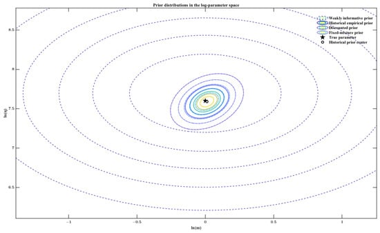
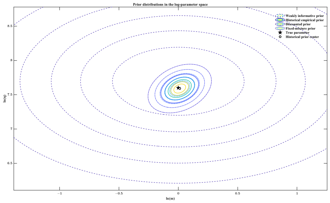
Figure 1 compares the concentration of the four priors in the log-parameter space.

Figure 1. Alternative prior models in the log-parameter space.

The priors progress from weak constraint to full borrowing, precision discounting, and mixture buffering. The empirical prior uses compatible historical information most efficiently. The discounted prior reduces historical precision by expanding its covariance, whereas the fixed mixture mitigates domination by an incorrect center through its weakly informative component. Subsequent experiments vary the center and strength separately to distinguish a misplaced prior from an overly influential prior.

3.2. Right-Censored Weibull Lifetime Model

For the current data set

$$D=\{(X_i,{\delta }_i):i=1,2,\dots ,n\}$$

(35)

the likelihood contribution is $f(X_i\mid m,\eta )$ for a failed unit and $R(X_i\mid m,\eta )$ for a right-censored unit. The right-censored likelihood is

$$L(m,\eta \mid D)={\displaystyle \prod _{i=1}^n}{\left[f(X_i\mid m,\eta )\right]}^{{\delta }_i}{\left[R(X_i\mid m,\eta )\right]}^{1-{\delta }_i}$$

(36)

Substituting the Weibull density and reliability functions gives

$$L(m,\eta \mid D)={\displaystyle \prod _{i=1}^n}{\left[{\displaystyle \frac{m}{\eta }}{\left({\displaystyle \frac{X_i}{\eta }}\right)}^{m-1}\right]}^{{\delta }_i}exp\left[-{\displaystyle \sum _{i=1}^n}{\left({\displaystyle \frac{X_i}{\eta }}\right)}^m\right]$$

(37)

For numerical stability, calculations use the log-likelihood

$$\ell (m,\eta \mid D)={\displaystyle \sum _{i=1}^n}{\delta }_i[lnm+(m-1)ln{X}_i-mln\eta ]-{\displaystyle \sum _{i=1}^n}{\left({\displaystyle \frac{X_i}{\eta }}\right)}^m$$

(38)

This likelihood uses the exact lifetime information from failed units and survival information from units still operating at censoring. All Bayesian methods use the same current-sample likelihood, providing a common data basis for comparing priors. Related analyses of non-homogeneous and interval-censored failure data show that Bayesian updating can combine a prior formed from general data with equipment-specific censored observations but that the value of the historical information depends on the compatibility between the model and the observation mechanism [38].

3.3. Posterior Model in the Log-Parameter Space

Equations (27) and (28) map $\mathit{\theta }$ uniquely to the Weibull parameters. The posterior in the log-parameter space is

$$\pi (\mathit{\theta }\mid D)={\displaystyle \frac{L(exp{\theta }_1,exp{\theta }_2\mid D)\pi \left(\mathit{\theta }\right)}{{\displaystyle {\int }_{\Theta }L(exp{\theta }_1,exp{\theta }_2\mid D)\pi \left(\mathit{\theta }\right)d\mathit{\theta }}}}$$

(39)

The prior $\pi \left(\mathit{\theta }\right)$ may be ${\pi }_0$, ${\pi }_H$, ${\pi }_{\alpha }$, or ${\pi }_M$, and $\Theta$ is the integration region in the log-parameter space. Because both the prior and posterior integration are defined in that space, no Jacobian for a transformation from the original parameter space is needed in Equation (39). A prior defined in the original parameter space would require the corresponding change-of-variables treatment.

3.4. Posterior Computation and Reliability Outputs

The posterior involves only two log parameters. Markov chain Monte Carlo can solve more general high-dimensional problems, but repeated Monte Carlo experiments with multiple priors would also require convergence diagnostics, effective-sample-size checks, and control of the sampling error, reducing cross-scenario reproducibility [39]. Deterministic two-dimensional grid integration is used instead. It directly yields normalized weights and numerical expectations for reliability quantities. Its validity depends on the grid covering essentially all posterior mass at sufficient resolution.

3.4.1. Numerical Solution of the Posterior

Let the integration region be

$$\Theta =[{\theta }_{1,min},{\theta }_{1,max}]\times [{\theta }_{2,min},{\theta }_{2,max}]$$

(40)

The two axes are divided into A and B grid points:

$${\theta }_{1a}={\theta }_{1,min}+(a-1){\Delta }_1,a=1,2,\dots ,A$$

(41)

$${\theta }_{2b}={\theta }_{2,min}+(b-1){\Delta }_2,b=1,2,\dots ,B$$

(42)

where

$${\Delta }_1={\displaystyle \frac{{\theta }_{1,max}-{\theta }_{1,min}}{A-1}},{\Delta }_2={\displaystyle \frac{{\theta }_{2,max}-{\theta }_{2,min}}{B-1}}$$

(43)

Grid point $(a,b)$ is

$${\mathit{\theta }}_{ab}={({\theta }_{1a},{\theta }_{2b})}^{\mathsf{T}}$$

(44)

with Weibull parameters

$$m_{ab}=exp\left({\theta }_{1a}\right),{\eta }_{ab}=exp\left({\theta }_{2b}\right)$$

(45)

The unnormalized log-posterior at that point is

$$q_{ab}=\ell (m_{ab},{\eta }_{ab}\mid D)+ln\pi \left({\mathit{\theta }}_{ab}\right)$$

(46)

To prevent numerical underflow, define

$$q_{max}=\underset{a,b}{max}{q}_{ab}$$

(47)

The normalized posterior weights are

$$w_{ab}={\displaystyle \frac{exp(q_{ab}-q_{max})}{{\displaystyle {\displaystyle \sum _{a=1}^A}{\displaystyle \sum _{b=1}^B}exp(q_{ab}-q_{max})}}}$$

(48)

and satisfy

$${\displaystyle \sum _{a=1}^A}{\displaystyle \sum _{b=1}^B}{w}_{ab}=1$$

(49)

For the fixed-mixture prior, Equation (46) uses

$$ln{\pi }_M\left({\mathit{\theta }}_{ab}\right)=ln[\omega {\pi }_H\left({\mathit{\theta }}_{ab}\right)+(1-\omega ){\pi }_0\left({\mathit{\theta }}_{ab}\right)]$$

(50)

3.4.2. Posterior Reliability Outputs

At each grid point,

$$m_{ab}=exp\left({\theta }_{1a}\right),{\eta }_{ab}=exp\left({\theta }_{2b}\right)$$

(51)

The Weibull mean lifetime is

$$\overline{T}=\eta \Gamma \left(1+{\displaystyle \frac{1}{m}}\right)$$

(52)

so at grid point $(a,b)$,

$${\overline{T}}_{ab}={\eta }_{ab}\Gamma \left(1+{\displaystyle \frac{1}{m_{ab}}}\right)$$

(53)

Posterior means provide point estimates:

$$\widehat{m}={\displaystyle \sum _{a=1}^A}{\displaystyle \sum _{b=1}^B}{m}_{ab}{w}_{ab}$$

(54)

$$\widehat{\eta }={\displaystyle \sum _{a=1}^A}{\displaystyle \sum _{b=1}^B}{\eta }_{ab}{w}_{ab}$$

(55)

and

$$\widehat{\overline{T}}={\displaystyle \sum _{a=1}^A}{\displaystyle \sum _{b=1}^B}{\overline{T}}_{ab}{w}_{ab}$$

(56)

At mission time t, the reliability at grid point $(a,b)$ is

$$R_{ab}\left(t\right)=exp\left[-{\left({\displaystyle \frac{t}{{\eta }_{ab}}}\right)}^{m_{ab}}\right]$$

(57)

and the posterior mean reliability is

$$\widehat{R}\left(t\right)={\displaystyle \sum _{a=1}^A}{\displaystyle \sum _{b=1}^B}{R}_{ab}\left(t\right)w_{ab}$$

(58)

For credibility level $1-\gamma$, the credible interval of any parameter function $g\left(\mathit{\theta }\right)$ is

$$\left[Q_{\gamma /2}\{g\left(\mathit{\theta }\right)\mid D\},Q_{1-\gamma /2}\{g\left(\mathit{\theta }\right)\mid D\}\right]$$

(59)

where $Q_p$ denotes the weighted posterior p-quantile computed from $w_{ab}$. Pointwise credible bands for the reliability function are obtained from the weighted distribution of $R_{ab}\left(t\right)$ at each mission time.

Engineering interpretation is strengthened by posterior probabilities of reliability thresholds. For mission time $t_j$ and reliability threshold $R_j^{*}$,

$$P\{R\left(t_j\right)\ge R_j^{*}\mid D\}={\displaystyle \sum _{a=1}^A}{\displaystyle \sum _{b=1}^B}I\{R_{ab}\left(t_j\right)\ge R_j^{*}\}{w}_{ab}$$

(60)

where $I(·)$ is the indicator function. For a mean-lifetime threshold ${\overline{T}}^{*}$,

$$P\{\overline{T}\ge {\overline{T}}^{*}\mid D\}={\displaystyle \sum _{a=1}^A}{\displaystyle \sum _{b=1}^B}I\{{\overline{T}}_{ab}\ge {\overline{T}}^{*}\}{w}_{ab}$$

(61)

Credible intervals quantify posterior uncertainty, while threshold probabilities quantify posterior support for engineering requirements. Both depend on the selected thresholds and the consequences of loss and should not be interpreted independently of mission-risk tolerance. They are nevertheless more suitable than a single point estimate for risk communication and maintenance decisions when failures are few and censoring is substantial [35]. Similar posterior probabilities and posterior-risk measures have been used to design reliability qualification tests for high-reliability space-propulsion systems under constraints on sample size, test duration, and cost [40].

3.5. Comparison Methods and Performance Metrics

Six methods are compared: the mean-rank method, bounded maximum likelihood, weak-prior Bayes, historical empirical Bayes, discounted Bayes, and fixed-mixture Bayes. The first two provide frequentist benchmarks, weak-prior Bayes provides a no-borrowing Bayesian benchmark, and the remaining methods represent full, discounted, and mixture borrowing.

Performance is assessed through parameter, lifetime, and reliability-function errors. For true parameters $m_0$ and ${\eta }_0$, the true mean lifetime is

$${\overline{T}}_0={\eta }_0\Gamma \left(1+{\displaystyle \frac{1}{m_0}}\right)$$

(62)

The relative errors of the shape parameter, scale parameter, and mean lifetime are

$$e_m={\displaystyle \frac{|\widehat{m}-m_0|}{m_0}}\times 100\%$$

(63)

$$e_{\eta }={\displaystyle \frac{|\widehat{\eta }-{\eta }_0|}{{\eta }_0}}\times 100\%$$

(64)

and

$$e_{\overline{T}}={\displaystyle \frac{|\widehat{\overline{T}}-{\overline{T}}_0|}{{\overline{T}}_0}}\times 100\%$$

(65)

On a mission-time grid $\{t_j:j=1,2,\dots ,J\}$, the reliability-function mean absolute error is

$$e_R={\displaystyle \frac{1}{J}}{\displaystyle \sum _{j=1}^J}|\widehat{R}\left(t_j\right)-R_0\left(t_j\right)|$$

(66)

where

$$R_0\left(t_j\right)=exp\left[-{\left({\displaystyle \frac{t_j}{{\eta }_0}}\right)}^{m_0}\right]$$

(67)

These metrics measure error in the failure-rate shape, lifetime scale, mean lifetime, and reliability curve across the mission-time range. Parameter and reliability errors need not move together, so the borrowing boundaries below jointly consider the scale-parameter relative error and reliability-function mean absolute error.

For M Monte Carlo replicates, the mean of any replicate-level error $e^{\left(r\right)}$ is

$$\overline{e}={\displaystyle \frac{1}{M}}{\displaystyle \sum _{r=1}^M}{e}^{\left(r\right)}$$

(68)

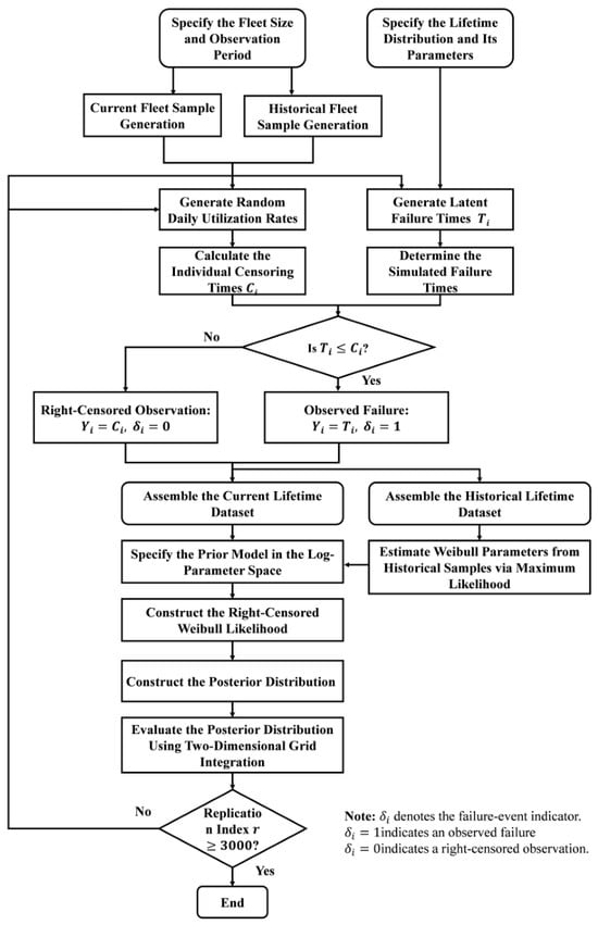
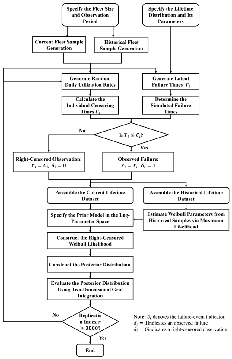
The workflow in Figure 2 is repeated for 3000 Monte Carlo replicates. Error metrics are averaged across replicates to reduce dependence on any representative sample. Figures illustrate representative responses, whereas methodological conclusions are based on the repeated-simulation summaries.

Figure 2. Simulation and posterior-assessment workflow.

4. Simulation Experiments and Sensitivity Analysis

The experiments have two levels. Historical borrowing is first evaluated when the historical and current samples are compatible, establishing whether it improves small-sample right-censored lifetime estimation. The historical prior center and precision are then misspecified to measure the sensitivity of posterior reliability metrics and calibrate prior-selection regions.

This study evaluates the effect of historical-information quality on reliability assessment from three perspectives: availability, observation completeness, and historical–current consistency. The historical-sample scale is examined by varying the number of batches used to construct the empirical prior; observation completeness is assessed under different censoring conditions; and inconsistency is examined through scale-parameter shifts and prior-misspecification scenarios.

All experiments use the data-generating assumptions in Section 2.1 and the same current-sample likelihood. The six estimators are compared using relative errors of the parameters and mean lifetime, reliability-function mean absolute error, posterior credible intervals, and posterior probabilities of reliability thresholds. Work on dynamic Bayesian networks and multilevel evidence fusion for hierarchical multistate systems likewise emphasizes the role of observation uncertainty in dynamic reliability updating [41].

4.1. Simulation Settings and Data-Constraint Checks

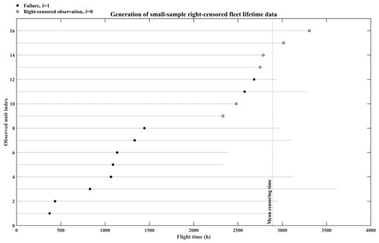
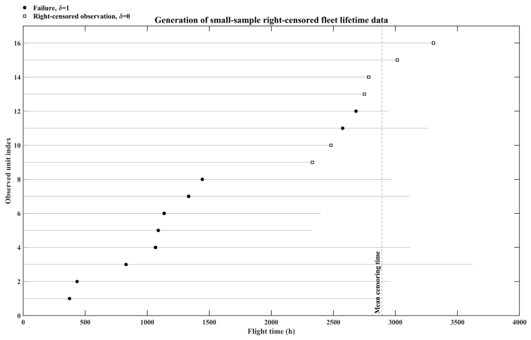
Current lifetimes follow the two-parameter Weibull distribution. A finite observation period and random daily utilization produce non-identical right-censoring times. Independent historical samples construct the empirical prior, while current samples are used only for posterior updating. Table 1 summarizes the sample-size and censoring constraints and the resulting historical-prior information. Figure 3 shows a representative current sample containing both failed and right-censored units with censoring times that vary with utilization. It confirms the intended data-generating mechanism; final performance conclusions rely on all 3000 simulation replicates.

Table 1. Constraints for small-sample right-censored data and historical prior information.

Quantity	Result
Current sample-size range	15–20
Mean current sample size	17.61
Censoring-proportion range	0.30–0.40
Mean censoring proportion	0.342
Valid historical sample groups	1200
Historical-prior mean of m	1.012
Historical-prior mean of $\eta$	1979.11
Proportion of valid historical samples	1.000

Figure 3. Failure and right-censored observations in a representative current sample.

Weak-prior Bayes is the Bayesian benchmark without historical borrowing. The empirical prior is constructed from independent historical lifetimes. The baseline discount factor is $\alpha =0.35$, and the historical-component weight in the fixed mixture is $\omega =0.80$. Both are prespecified analytical settings for this simulation. In particular, $\omega =0.80$ provides a fixed-mixture robustness reference; it is not a universally optimal value estimated from the current data.

In the proposed assessment framework, $\alpha$ and $\omega$ are not independent tuning parameters; they control the degree of historical-information borrowing and should be selected with reference to the consistency level and the corresponding borrowing region. The baseline settings represent partial borrowing and fixed-mixture correction, respectively, and are not claimed to be optimal for every engineering application.

The evaluation includes relative errors in the shape parameter, scale parameter, and mean lifetime together with the reliability-function mean absolute error. For the Bayesian methods, parameter credible intervals, reliability-function credible bands, and posterior threshold probabilities are also compared. These quantities evaluate point accuracy, posterior uncertainty, and support for engineering thresholds.

4.2. Feasibility Under Compatible Historical Information

The compatible scenario asks whether full historical borrowing can stabilize small-sample right-censored assessment without materially increasing the mean error when the historical and current fleets follow the same lifetime distribution.

Table 2 reports average errors over 3000 replicates. The mean-rank and bounded maximum-likelihood estimators have relatively large parameter and mean-lifetime errors when few failures are available. Weak-prior Bayes produces a full posterior, but the current likelihood constrains the scale poorly, and the posterior mean lifetime is sensitive to its long upper tail. Its mean-lifetime error is consequently high in this scenario. Historical empirical Bayes combines the historical parameter distribution with the current censored likelihood. Its relative errors for the shape parameter, scale parameter, and mean lifetime are 2.52%, 3.54%, and 3.12%, respectively, and its reliability-function mean absolute error is 1.28%. Discounted and fixed-mixture Bayes intentionally reduce the influence of the fully informative historical prior. Their errors are therefore somewhat larger under exact compatibility but remain substantially below those of the no-borrowing benchmarks.

Table 2. Mean estimation errors under compatible historical information.

Method	${\mathit{RE}}_{\mathit{m}}$	${\mathit{RE}}_{\mathit{\eta }}$	${\mathit{RE}}_{\mathit{\mu }}$	${\mathit{MAE}}_{\mathit{R}}$
Mean-rank method	29.44%	34.26%	40.80%	14.47%
Bounded maximum likelihood	19.42%	33.03%	39.59%	8.87%
Weak-prior Bayes	17.51%	41.91%	70.24%	9.93%
Empirical Bayes	2.52%	3.54%	3.12%	1.28%
Discounted Bayes	5.17%	9.27%	9.48%	3.11%
Fixed-mixture Bayes	3.93%	6.42%	9.49%	2.10%

Under the compatible, independent, and non-informative-censoring conditions considered here, the historical empirical prior compensates effectively for limited failures in the current sample and maintains low average error across replicates. This conclusion cannot be inferred from one representative sample, and historical observations from nominally identical equipment are not necessarily compatible in field applications.

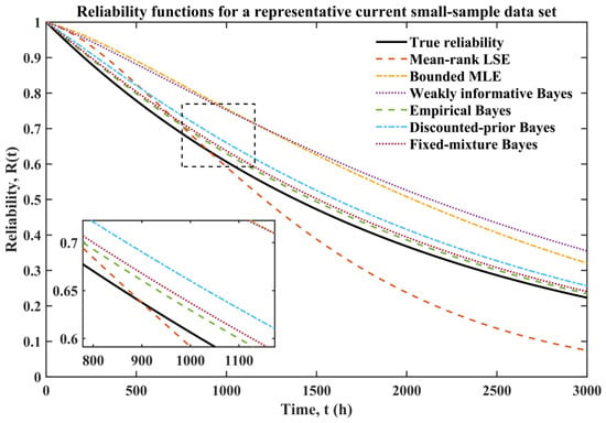
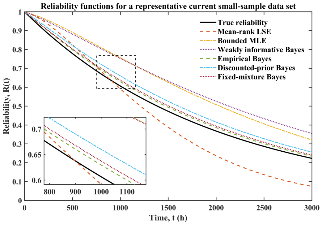
Figure 4 compares reliability curves for a representative current sample. Among the six methods, the empirical Bayes curve is closest to the true reliability curve.

Figure 4. Reliability estimates under different methods for the current sample.

4.3. Posterior Uncertainty and Reliability-Threshold Probabilities

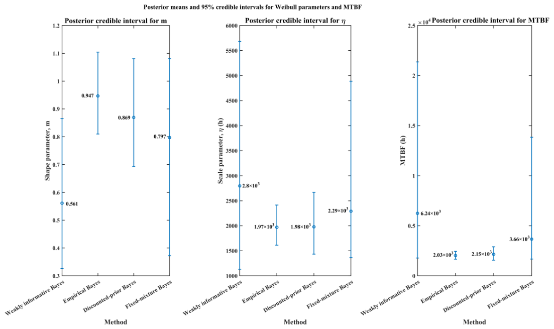
Bayesian assessment provides posterior uncertainty in addition to improved point estimates under an effective prior. At the 95% credibility level, the mean widths of the scale-parameter and mean-lifetime credible intervals are 830.28 and 787.86 for empirical Bayes compared with 3575.54 and 6302.54 for weak-prior Bayes. Compatible historical information therefore narrows posterior intervals substantially. A narrower interval indicates useful information only when accompanied by low bias or satisfactory coverage; narrowness alone is not evidence of a reliable method. High-reliability lifetime studies of critical aeronautical structures similarly show that point estimates alone do not support high-reliability claims; posterior or confidence intervals are also needed to represent tail-lifetime uncertainty [42].

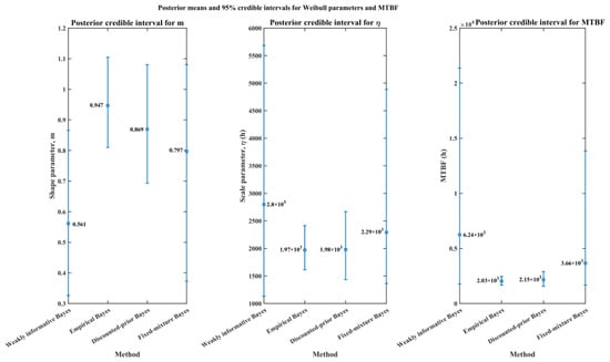
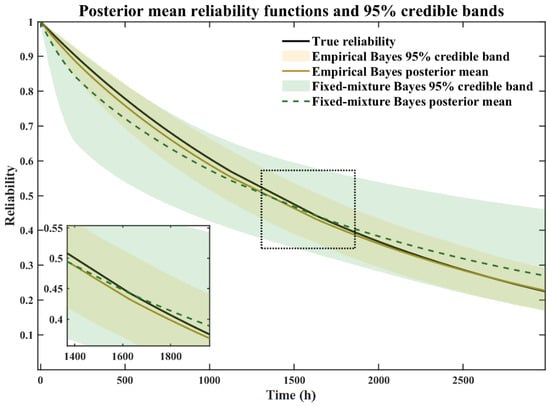
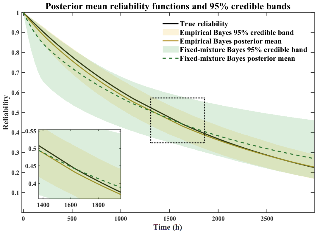
Figure 5 compares the posterior means and 95% credible intervals of the shape parameter m, scale parameter $\eta$, and mean lifetime. The empirical Bayes posterior is centered near the true values and is most concentrated. The discounted and fixed-mixture priors yield moderately wider intervals, showing the accuracy–robustness tradeoff created by relaxing historical constraints. Figure 6 presents the corresponding uncertainty in the reliability assessment.

Figure 5. Posterior means and 95% credible intervals of Weibull parameters and mean lifetime.

Figure 6. Posterior mean and 95% credible band under compatible historical information.

To more comprehensively evaluate the effect of historical borrowing on posterior uncertainty assessment, Monte Carlo coverage probabilities of the 95% credible intervals are calculated for the Weibull parameters, mean lifetime, and mission reliability $R\left(500\right)$ under different historical-information states. The results in Table 3 show that the historical empirical prior substantially reduces credible interval widths under compatibility, but its coverage is more sensitive to prior shifts because of the stronger information constraint. The weak prior maintains higher coverage because it imposes weaker historical constraints, although this comes at the cost of lower estimation efficiency. The discounted prior provides a balance between estimation efficiency and uncertainty calibration. When historical information is shifted, discounting can mitigate the coverage reduction caused by full historical borrowing, indicating that appropriately controlling the influence of historical information is important for robust Bayesian reliability assessment.

Table 3. Mod5% Bayesian credible intervals under different historical-information states.

Historical-Information State	Scale Shift	Method	m Coverage	$\mathit{\eta }$ Coverage	Mean-Lifetime Coverage	$\mathit{R}\left(500\right)$ Coverage
Compatible historical information	1.0	Weak prior	0.952	0.952	0.952	0.956
Compatible historical information	1.0	Historical empirical prior	0.924	0.924	0.924	0.938
Compatible historical information	1.0	Discounted prior	0.954	0.954	0.950	0.960
Historical scale low	0.8	Weak prior	0.937	0.959	0.940	0.959
Historical scale low	0.8	Historical empirical prior	0.884	0.841	0.800	0.929
Historical scale low	0.8	Discounted prior	0.939	0.937	0.914	0.948
Historical scale high	1.2	Weak prior	0.950	0.961	0.952	0.954
Historical scale high	1.2	Historical empirical prior	0.928	0.902	0.914	0.936
Historical scale high	1.2	Discounted prior	0.958	0.959	0.960	0.964

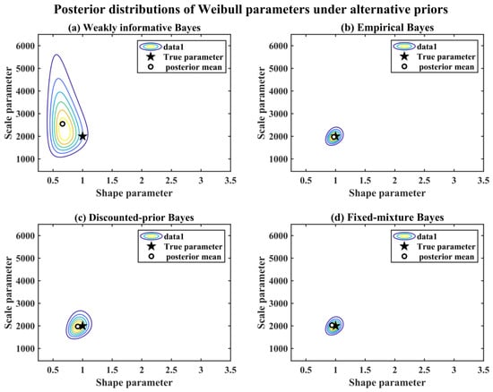
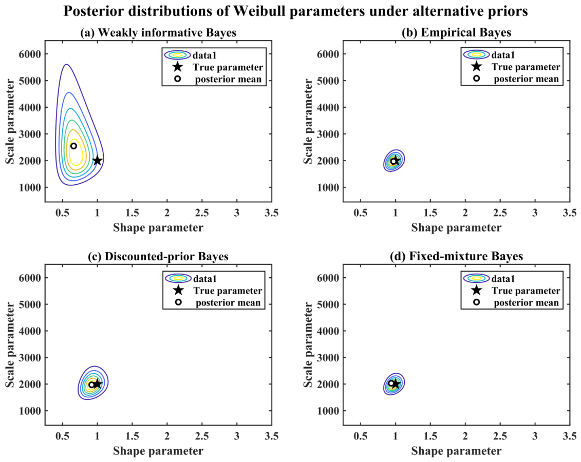
Figure 7 shows joint posterior contours for m and $\eta$ under the four priors. The weak-prior posterior covers a broad region, indicating that the current small sample cannot distinguish the parameters precisely. The empirical Bayes posterior is the most concentrated and is centered near the true parameters. The discounted and fixed-mixture posteriors have intermediate concentration. The contours also reveal posterior dependence between m and $\eta$; marginal means alone do not characterize that uncertainty.

Figure 7. Joint posterior distributions of Weibull parameters under alternative priors.

Parameter credible intervals, joint posterior contours, and reliability-function credible bands are therefore considered together rather than judging historical borrowing from a single parameter estimate.

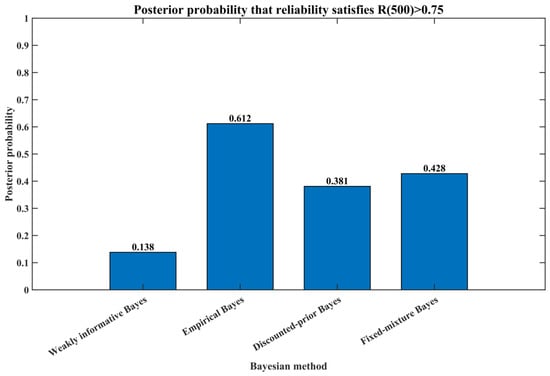
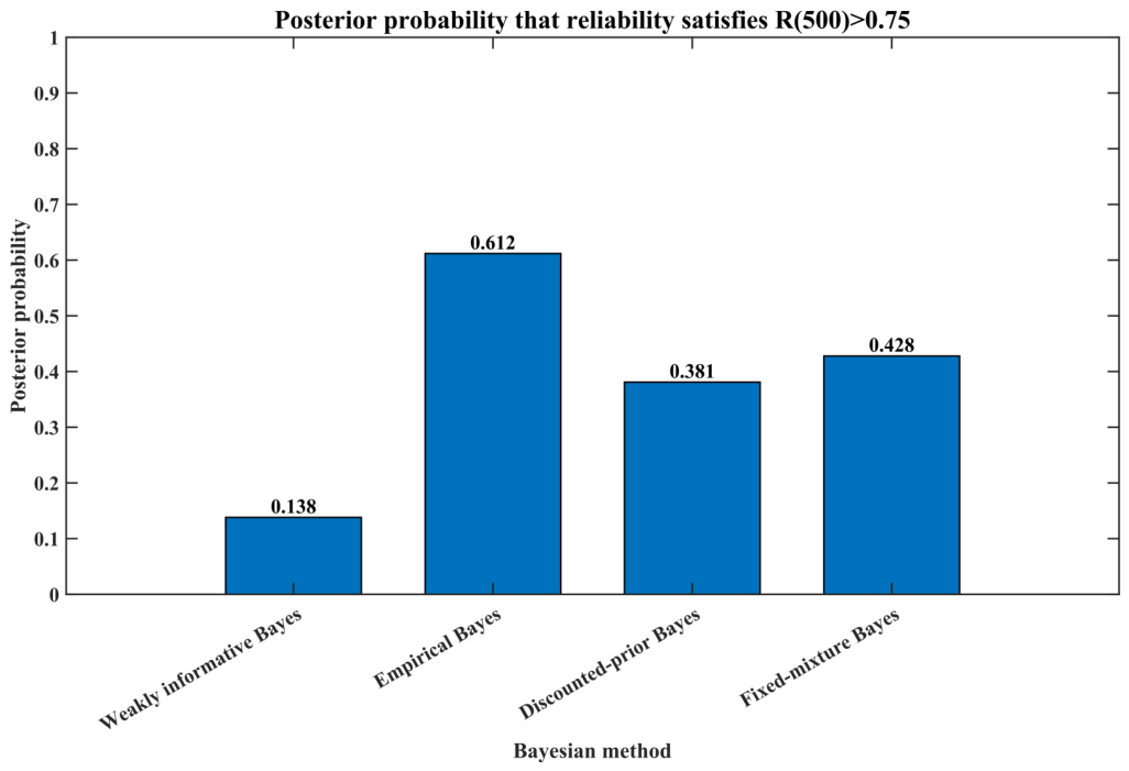
Posterior threshold probabilities quantify support for reliability requirements and supplement comparisons of borrowing strategies. Figure 8 shows the posterior probability of the illustrative requirement $R\left(500\right)>0.75$. Borrowing strength changes the posterior support materially. Empirical Bayes produces the highest probability, indicating that full borrowing strengthens support for the reliability requirement when historical and current information are compatible.

Figure 8. Posterior probability that reliability satisfies R(500) > 0.75.

4.4. Sensitivity and Robustness

The Weibull shape parameter m characterizes the trend in the failure rate over service time, whereas the scale parameter $\eta$ characterizes the overall lifetime level. For equipment with a common failure mechanism, differences in batch, mission profile, environmental stress, or maintenance may first appear as changes in lifetime scale. To isolate that effect, the controlled sensitivity analysis holds the shape-prior center fixed and shifts only the scale-prior center. When a historical prior conflicts with current data, borrowing benefit, estimation error, and decision loss involve a material tradeoff; systematic sensitivity analysis is therefore needed to assess the robustness of a borrowing strategy [43]. Because historical-information quality directly affects the performance of Bayesian information borrowing, this section also examines its effects from the perspectives of consistency and availability. Robustness is evaluated by varying historical-sample accumulation, historical–current parameter shifts, and prior–data conflict.

4.4.1. Empirical-Prior Uncertainty Under Finite Historical Information

To test whether the proposed method depends on the amount of available historical information under historical-current compatibility, an additional finite-historical-batch scenario is considered. The empirical prior is re-estimated from a single historical batch, three historical batches, and ten historical batches, respectively, and Bayesian updating is then performed under the condition that historical information is compatible with the current object.

The stability of the empirical-prior center is first examined. Table 4 reports the uncertainty of the prior-center estimates for the shape parameter, scale parameter, and $R\left(500\right)$ under different numbers of historical batches. The results show clear sampling fluctuation in the prior center when only one historical batch is available. As the number of historical batches increases, the standard deviations of all prior-center errors decrease continuously, indicating that finite historical data do introduce additional prior-estimation uncertainty, whereas historical-information accumulation gradually improves the stability of the empirical prior. Therefore, in practical engineering applications, an empirical prior should not be simply assumed to be an accurate prior; the finite size of historical data should be considered.

Table 4. Uncertainty analysis of empirical-prior centers under different historical-information sizes.

Historical-Information Scenario	Historical Batches	SD of Shape-Center Error	SD of Scale-Center Relative Error	SD of Prior-Center $\mathit{R}\left(500\right)$ Error
Single historical batch	1	0.357887	0.120	0.080202
Finite historical batches	3	0.170739	0.075	0.047532
Finite historical batches	10	0.088261	0.041	0.025761

On this basis, Table 5 further evaluates the effect of finite historical batches on posterior reliability-assessment performance. The results show that the mean error of $R\left(500\right)$ remains small under one, three, and ten historical batches without obvious systematic bias. As the number of historical batches increases, both RMSE and prior-center variation decrease, while the 95% credible interval coverage generally remains close to the nominal level. The stability of posterior reliability assessment is especially improved when three or ten historical batches are available.

Table 5. Reliability-assessment performance under different historical-information sizes with the historical empirical prior.

Historical-Information Scenario	$\mathit{R}\left(500\right)$ Mean Error	$\mathit{R}\left(500\right)$ RMSE	$\mathit{R}\left(500\right)$ Coverage	Prior-Center $\mathit{R}\left(500\right)$ SD
Single historical batch	−0.001517	0.064161	0.934000	0.075412
Three historical batches	−0.001925	0.046988	0.934000	0.044790
Ten historical batches	−0.000457	0.032000	0.944000	0.024356

These results indicate that compared with abundant historical information, finite historical batches reduce the precision of the empirical prior. Nevertheless, under compatible historical information, the proposed method still maintains small reliability-assessment bias and reasonable uncertainty coverage with performance improving as historical information accumulates. Therefore, the borrowing benefit observed in the compatible scenario is not solely caused by an “unusually accurate prior center” formed from a large number of historical fleets; the framework remains applicable under finite historical information.

4.4.2. Sensitivity to Historical Scale Shift

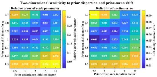
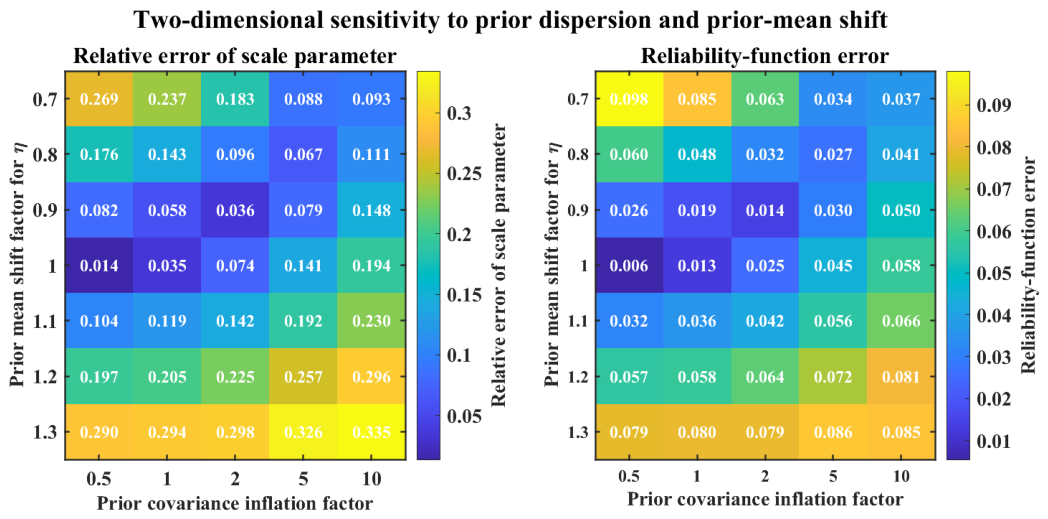
The historical scale-shift factor is the ratio of the historical prior’s scale center to the true current scale. It represents historical underestimation, compatibility, or overestimation of the current lifetime level. Scale-parameter errors are compared for empirical, discounted, and fixed-mixture Bayes, while Figure 9 also examines the reliability-function error.

Figure 9. Two-dimensional sensitivity of parameter-estimation and reliability-prediction errors to prior-mean shift and variance inflation.

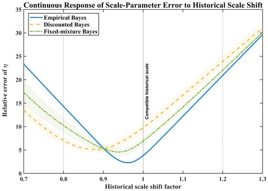
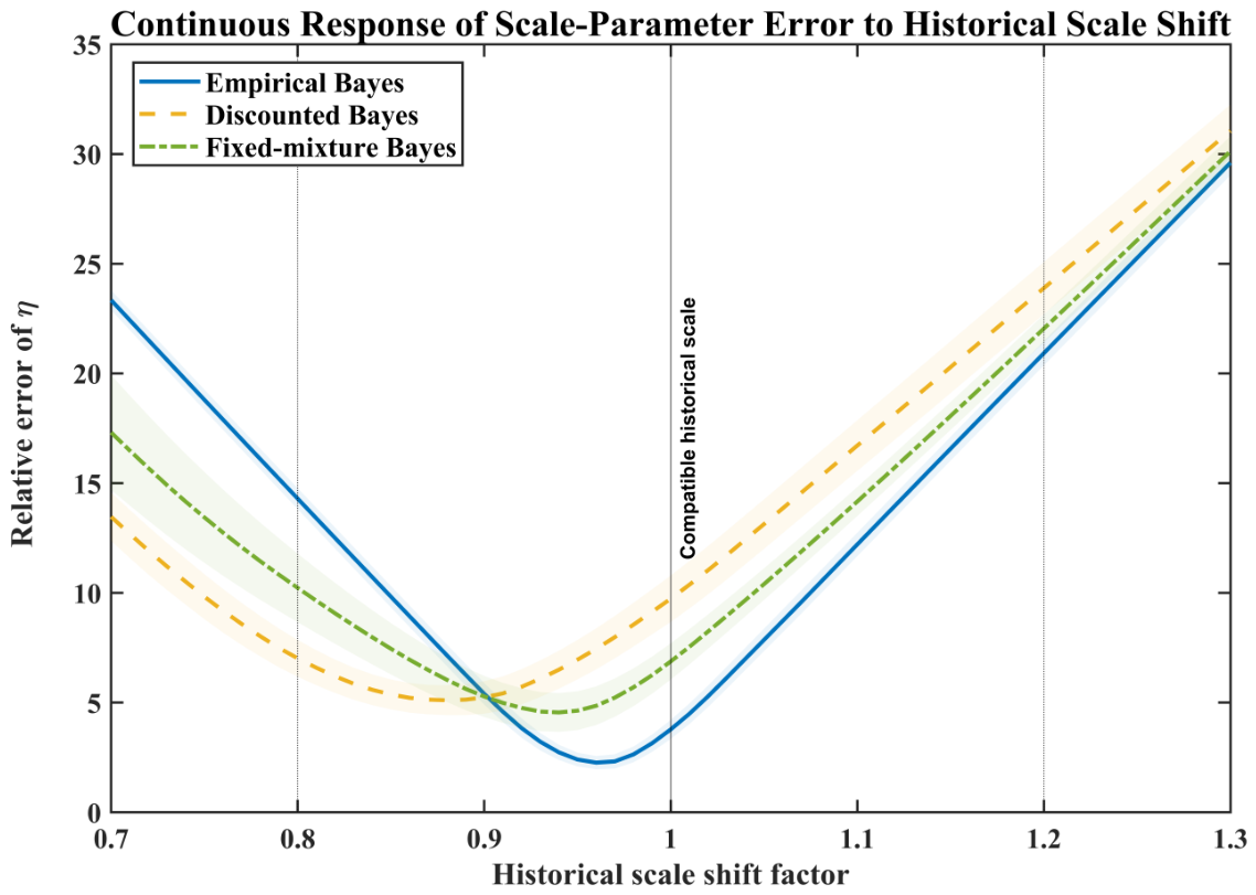
Figure 10 shows that the scale-parameter relative errors of all three borrowing priors respond to shifts in the historical scale center. At a shift factor of 1.0, empirical Bayes has the lowest error. When the factor falls to 0.8, its error increases to 14.34% compared with 6.71% for discounted Bayes and 9.29% for fixed-mixture Bayes. Thus, if historical lifetimes underestimate the current lifetime level, reducing prior precision or introducing a weakly informative component limits the pull of an incorrect center on the posterior scale estimate.

Figure 10. Continuous response of scale-parameter relative error to historical scale shift.

With larger shifts, the posterior center under the full empirical prior follows the historical center. The discounted prior reduces prior precision through covariance inflation, while the fixed mixture provides alternative posterior mass through its weakly informative component.

The scale-parameter error remains generally low for shift factors near 0.9–1.1. At shifts of approximately 20% or more, differences among methods and sensitivity to prior misspecification become pronounced. Optimistic historical shifts deserve particular attention. If historical data come from a fleet with lower utilization, better maintenance, or milder mission profiles, full borrowing may overestimate current lifetime and mission reliability. That consequence is typically more serious than conservative underestimation. When systematic differences in provenance are present, weaker borrowing should be preferred and the posterior should be interpreted against mission-risk tolerance.

4.4.3. Discount Factor and Prior Strength

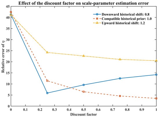
The discount factor $\alpha$ controls historical precision. For $0<\alpha \le 1$, the discounted covariance is ${\mathbf{\Sigma }}_H/\alpha$; $\alpha =1$ is the full empirical prior, and a smaller $\alpha$ weakens historical information. In Table 6 and Figure 11, $\alpha =0$ is the limiting no-borrowing reference implemented with the weakly informative prior, which is not obtained by substituting zero into ${\mathbf{\Sigma }}_H/\alpha$. The values examined are 0, 0.25, 0.50, 0.75, and 1.00.

Table 6. Joint effects of historical scale shift and discount factor on scale-parameter relative error.

Historical Scale-Shift Factor	$\mathit{\alpha }=0$	$\mathit{\alpha }=0.25$	$\mathit{\alpha }=0.50$	$\mathit{\alpha }=0.75$	$\mathit{\alpha }=1.00$
0.8	41.31%	5.89%	9.57%	12.50%	14.19%
1.0	42.46%	11.43%	6.50%	4.57%	3.48%
1.2	41.14%	24.20%	22.63%	21.06%	20.50%

Figure 11. Effects of the discount factor on parameter-estimation errors.

Table 6 reports the mean scale-parameter relative error for combinations of historical scale shift and discount factor. Under compatibility, increasing $\alpha$ continuously reduces error. When the prior center is low by 20%, $\alpha =0.25$ gives the lowest error, 5.89%, and larger values increase the error. When the prior center is high by 20%, errors remain large for every fixed $\alpha$. Adjusting precision alone cannot remove a substantial center shift.

Figure 9 shows the two-dimensional joint effects of prior-center shift and covariance inflation. The left panel gives the scale-parameter relative error, and the right panel gives the reliability-function error. Full borrowing is most accurate when the shift factor is close to 1.0 and the prior variance is small. As the center shifts, moderate covariance inflation reduces its influence. Excessive inflation, however, discards useful historical information and cannot remove the systematic error caused by a large shift.

Figure 11 confirms that the effect of $\alpha$ depends on the historical center. A large $\alpha$ uses historical information efficiently under compatibility. A moderate value is preferable when the historical scale is underestimated. If the historical scale is overestimated by 20%, every fixed value still gives a high error. There is no universally optimal discount factor independent of historical–current compatibility.

Increasing $\alpha$ improves accuracy and narrows posterior intervals under compatibility, but it strengthens the influence of an incorrect historical center under shift. Decreasing $\alpha$ improves robustness but weakens the information added to a small sample. The discount factor therefore represents an accuracy–robustness tradeoff rather than a quantity to maximize or minimize.

The baseline value $\alpha =0.35$ provides a compromise when compatibility is unknown in this simulation. It is scenario-specific rather than a universal value for other equipment systems. Field applications should recalibrate it using historical provenance, conflict diagnostics, and the losses associated with incorrect decisions.

4.4.4. Prior-Misspecification Stress Tests

Additional stress scenarios include low and high historical scale centers, an overly narrow prior, an overly broad prior, and a misspecified shape parameter. Heavy-tailed and bimodal mixture priors provide supplementary comparisons of whether alternative components buffer prior conflict. The purpose of fixed or dynamic mixtures is to limit excessive borrowing from conflicting historical information, and the robust component and its weight should be calibrated against the allowable degree of error inflation [37].

As can be seen from Table 7, the compatible empirical prior has low error, but scale and mean-lifetime errors rise quickly when the historical scale center is substantially shifted or an incorrect prior is overly narrow. Increasing prior variance weakens the pull of an incorrect center but also reduces information efficiency. Heavy-tailed and bimodal mixtures have lower errors in some conflict scenarios, indicating that an alternative component can improve robustness.

Table 7. Estimation errors and auxiliary posterior-risk indicators under prior-misspecification stress tests.

Prior Scenario	${\mathit{MARE}}_{\mathit{\eta }}$	${\mathit{MARE}}_{\mathbf{mean} \mathbf{lifetime}}$	Posterior-Risk Indicator
Correct empirical prior	0.0366	0.0322	0.0191
Low scale center, 0.7	0.2349	0.2350	0.0933
High scale center, 1.3	0.2918	0.2928	0.0807
Scale center 0.7 and overly narrow prior	0.2873	0.2897	0.1206
Scale center 0.7 and overly broad prior	0.0822	0.0566	0.0998
Misspecified shape parameter	0.0440	0.0588	0.1551
Heavy-tailed mixture prior	0.0659	0.1011	0.0492
Bimodal mixture prior	0.0330	0.0273	0.0290

Across scenarios, weak-prior Bayes avoids attraction to an incorrect historical center but has a broad posterior. Discounted Bayes mitigates moderate shift, and fixed-mixture Bayes retains a larger buffer under marked conflict. The stress tests assess whether these prior-selection directions are reasonable; the three borrowing regions are still calibrated principally by the scale-parameter relative error and reliability-function mean absolute error.

Within the simulated range, a historical empirical prior is appropriate for compatible and credible information, a discounted prior is appropriate for a moderate shift that retains borrowing value, and a fixed-mixture prior is appropriate under substantial shift or high misspecification risk. This progression motivates the offline boundary calibration.

4.5. Historical-Information Borrowing-Region Calibration and Threshold Sensitivity Analysis

When historical information is used for reliability assessment, the effective use of historical data mainly depends on the consistency between the historical information and the current sample. If the two are highly consistent, the full use of historical information can reduce parameter-estimation uncertainty under small-sample conditions. If historical information is shifted, excessive borrowing may move the posterior distribution in an incorrect direction and reduce reliability assessment accuracy. Therefore, this study constructs a borrowing-region classification method that reflects the degree of historical-information consistency.

The borrowing-region thresholds are not treated as fixed engineering rules specified in advance but rather are calibrated offline from Monte Carlo simulation results. The joint evaluation criteria are the relative error of the Weibull scale parameter and the mean absolute error of the reliability function. The scale-parameter error describes bias in the estimated lifetime level, whereas the reliability-function error describes prediction bias over the mission-time range. For the rth Monte Carlo replicate, the joint error criterion is defined as

$$J_r=max\{E_{\eta ,r},E_{R,r}\}$$

(69)

where

$$E_{\eta ,r}={\displaystyle \frac{|{\widehat{\eta }}_r-{\eta }_0|}{{\eta }_0}}$$

(70)

and

$$E_{R,r}={\displaystyle \frac{1}{K}}{\displaystyle \sum _{k=1}^K}|{\widehat{R}}_r\left(t_k\right)-R_0\left(t_k\right)|.$$

(71)

The relevant symbols and their meanings are provided in Table 8.

Table 8. Notation for borrowing-region calibration and threshold sensitivity analysis.

Symbol	Meaning
r	Index of the rth Monte Carlo replicate
${\eta }_0$	True Weibull scale parameter
${\widehat{\eta }}_r$	Posterior estimate of the scale parameter in replicate r
$E_{\eta ,r}$	Relative error of the scale parameter
$t_k$	kth mission-time point
$R_0\left(t_k\right)$	True reliability at $t_k$
${\widehat{R}}_r\left(t_k\right)$	Posterior reliability estimate at $t_k$
$E_{R,r}$	Mean absolute error of the reliability function
$J_r$	Joint error criterion
${\tau }_1,{\tau }_2$	Two-level error thresholds

Using the maximum error as the joint criterion ensures that the borrowing strength is adjusted whenever either evaluation metric shows a large deviation. Given a threshold pair $({\tau }_1,{\tau }_2)$, the three historical-information borrowing regions are defined as follows:

$$J_r\le {\tau }_1$$

(72)

indicates that the historical information is highly consistent with the current data and the full-borrowing strategy is used;

$${\tau }_1<J_r\le {\tau }_2$$

(73)

indicates that the historical information has a certain degree of shift and the discounted-borrowing strategy is used;

$$J_r>{\tau }_2$$

(74)

indicates relatively high historical-information uncertainty and the fixed-mixture correction strategy is used. Because these error metrics depend on the true parameters in the Monte Carlo simulation, the region classification is an offline simulation-calibrated region. Its role is to reveal how borrowing strategies vary under different levels of historical-information consistency, and it cannot be used directly as an online classifier for field data.

4.5.1. Sensitivity Analysis of Threshold Combinations

To avoid dependence on a single threshold setting, three candidate threshold combinations are considered:

$$({\tau }_1,{\tau }_2)=(5\%,15\%)$$

(75)

$$({\tau }_1,{\tau }_2)=(10\%,20\%)$$

(76)

$$({\tau }_1,{\tau }_2)=(15\%,25\%).$$

(77)

A smaller threshold corresponds to a stricter information-borrowing requirement, which can reduce the risk of erroneous borrowing but may also limit the use of valuable historical information. A larger threshold allows more historical information to enter the full-borrowing region but may increase potential shift risk. To quantitatively evaluate the effect of different threshold combinations, the empirical distribution function of the joint error is defined as

$${\widehat{F}}_J\left(\tau \right)={\displaystyle \frac{1}{N}}{\displaystyle \sum _{r=1}^N}I(J_r\le \tau ),$$

(78)

where N is the number of Monte Carlo replicates; ${\widehat{F}}_J\left({\tau }_1\right)$ denotes the proportion of samples entering the full-borrowing region, and ${\widehat{F}}_J\left({\tau }_2\right)$ denotes the cumulative proportion whose joint error does not exceed the upper threshold.

Mean estimation error describes overall borrowing performance but does not fully capture the uncertainty and directional risks introduced by historical information. In aeronautical reliability assessment, optimistic historical information can lead to reliability overestimation, which is a risk with particular engineering importance. We therefore supplement the symmetric error criteria with an asymmetric positive-error risk indicator to assess reliability overestimation and inform borrowing-region calibration.

Excessive historical-information borrowing may optimistically overestimate mission reliability and thereby affect practical failure-risk assessment. We therefore introduce the positive-error risk as an auxiliary asymmetric reliability-risk measure. It is the proportion of all Monte Carlo trials in which the posterior estimate of reliability exceeds the true reliability by more than the first threshold ${\tau }_1$.

For a given first threshold ${\tau }_1$, positive-error risk is defined as

$$P_{+}\left({\tau }_1\right)={\displaystyle \frac{1}{N}}{\displaystyle \sum _{r=1}^N}I[{\widehat{R}}_r\left(500\right)-R_{0,r}\left(500\right)>{\tau }_1].$$

(79)

4.5.2. Threshold Selection and the Balance Between Information Use and Risk

Table 9 reports sensitivity-analysis results for different historical-information borrowing thresholds. With the 5–15% combination, erroneous borrowing is strictly controlled, but much useful historical information is excluded, which is unfavorable for small-sample reliability assessment. With the 10–20% combination, the full-borrowing proportion rises to 81.18%, the fixed-mixture-region proportion falls to 0.98%, and the positive-error risk decreases to 3.10%. With the 15–25% combination, the full-borrowing proportion rises further to 94.87%, assigning nearly all simulated samples to full borrowing; the discounted-borrowing and fixed-mixture regions fall to 4.98% and 0.15%, respectively. Although this more permissive combination reduces the probability of exceeding the error limit, it also weakens the classification’s ability to identify moderate historical shifts. Overall, the 10–20% combination offers a better balance between historical-information use and erroneous-borrowing control.

Table 9. Sensitivity analysis under different historical-information borrowing threshold combinations.

Threshold Combination	Full-Borrowing Region	Discounted-Borrowing Region	Fixed-Mixture Region	${\widehat{\mathit{F}}}_{\mathit{J}}\left({\mathit{\tau }}_1\right)$	${\widehat{\mathit{F}}}_{\mathit{J}}\left({\mathit{\tau }}_2\right)$	${\mathit{P}}_{+}\left({\mathit{\tau }}_1\right)$
5–15%	≤5%	5–15%	>15%	0.492476	0.948667	0.190381
10–20%	≤10%	10–20%	>20%	0.811810	0.990190	0.031048
15–25%	≤15%	15–25%	>25%	0.948667	0.998476	0.002000

Considering historical-information use, region-discrimination capability, and erroneous-borrowing risk together, we adopt the 10–20% threshold combination as the information-borrowing-region criterion. This combination is not claimed to have universal statistical meaning; it represents a sensitivity region obtained from the joint error distribution under the sample size, right-censoring, Weibull lifetime model, and reliability-assessment objective considered in this study.

This section constructs a borrowing-region calibration method based on the joint error criterion and verifies the stability of the region classification through threshold-combination sensitivity analysis. The results show that the 10–20% threshold combination provides a good balance between historical-information use and erroneous-borrowing risk and is therefore used as the recommended borrowing region under the simulation conditions of this study. In practical engineering scenarios, however, this threshold should still be further calibrated according to equipment type, sample size, and risk tolerance. Future work will further investigate the reliability assessment of aeronautical equipment using real operating data and complex real-world operating conditions.

5. Conclusions

This paper addresses the limited current data and the difficulty of quantifying the degree of historical-information borrowing in small-sample right-censored lifetime assessment of aeronautical equipment. A Bayesian reliability assessment framework incorporating historical information is proposed. Based on a two-parameter Weibull lifetime model, weakly informative, historical empirical, discounted, and fixed-mixture priors are constructed in the log-parameter space, and historical information is fused with current observations through the right-censored likelihood. By constructing mutually independent historical and current fleet simulation scenarios, the study systematically analyzes how historical-information compatibility, finite historical batches, historical scale shifts, borrowing-strength variation, and prior misspecification affect the performance of reliability assessment. On this basis, a joint criterion based on scale-parameter error and reliability-function error is used to conduct threshold sensitivity analysis and to form borrowing regions under different levels of historical-information consistency, providing an analytical basis for selecting the degree of historical-information borrowing.

The results show that when historical and current information are compatible, the reasonable borrowing of historical information can effectively reduce parameter-estimation error and posterior uncertainty under small-sample conditions. When only finite historical batches are available, the empirical-prior center has increased uncertainty, but the posterior reliability assessment still maintains small bias and reasonable interval coverage, indicating that the proposed reliability assessment method has good applicability under finite historical information in the constructed fleet simulation scenario. When historical information is shifted, full borrowing pulls posterior estimates toward an incorrect prior center, whereas the discounted prior and fixed-mixture prior, which reduce the weight of historical information, can alleviate this effect to some extent. The final threshold sensitivity analysis shows that the degree of historical-information borrowing should be adjusted according to historical-current information consistency. The borrowing regions obtained in this study describe information-use patterns under different consistency levels and should not be interpreted as universal fixed engineering boundaries.

This paper still has limitations. The current analysis is mainly based on a Weibull lifetime model and the constructed fleet simulation scenario, focusing on historical-information compatibility, finite historical batches, and scale-parameter shifts. It does not fully cover more complex engineering scenarios such as competing failures, maintenance renewal, multisource historical-data heterogeneity, mission-environment changes, or joint multi-parameter shifts in historical information. The borrowing regions and thresholds are mainly calibrated using error metrics in simulation, while true parameters cannot be directly observed in field data; therefore, they cannot yet be regarded as fixed engineering rules ready for direct deployment. Future research will combine real operating data with observable prior–data conflict diagnostics, and it will further introduce hierarchical Bayesian, multisource information-fusion, and adaptive prior-borrowing mechanisms to dynamically calibrate discount strength and mixture weights, thereby improving the applicability and engineering implementability of the proposed method in the reliability assessment of complex aeronautical equipment.

References

- Liu, Q.; Huang, X.P.; Zhou, J.L.; Jin, G.; Sun, Q. Bayesian reliability evaluation of a momentum wheel based on physics of failure. Acta Aeronaut. Astronaut. Sin. (In Chinese) 2009, 30, 1392–1397. [Google Scholar]
- Song, Z.Y.; Fang, Z.G.; He, W.L.; Sun, Y.K.; Wang, Z.; Li, C.X.; Liu, S.F. Bayesian small-sample reliability assessment for launch vehicles. J. Deep Space Explor. (In Chinese) 2021, 8, 62–69. [Google Scholar]
- Liu, M.; Zheng, H.; Yang, J. Reliability evaluation for Weibull distribution with heavily Type II censored data. Qual. Reliab. Eng. Int. 2024, 40, 3620–3642. [Google Scholar] [CrossRef] [Scilit]
- Liu, T.; Zhang, L.; Jin, G.; Pan, Z.Q. Reliability assessment of heavily censored data based on E-Bayesian estimation. Mathematics 2022, 10, 4216. [Google Scholar] [CrossRef] [Scilit]
- Tan, Y.; Zhao, Q.; Wang, W.F.; Guo, B.; Jiang, P. Type-I censored reliability acceptance test design for Weibull products considering expert information. Syst. Eng. Electron. (In Chinese) 2022, 44, 1409–1416. [Google Scholar]
- Jia, X. Reliability analysis for Weibull distribution with homogeneous heavily censored data based on Bayesian and least-squares methods. Appl. Math. Model. 2020, 83, 169–188. [Google Scholar] [CrossRef] [Scilit]
- Ducros, F.; Pamphile, P. Bayesian estimation of Weibull mixture in heavily censored data setting. Reliab. Eng. Syst. Saf. 2018, 180, 453–462. [Google Scholar] [CrossRef] [Scilit]
- Shuto, S.; Amemiya, T. Sequential Bayesian inference for Weibull distribution parameters with initial hyperparameter optimization for system reliability estimation. Reliab. Eng. Syst. Saf. 2022, 224, 108516. [Google Scholar] [CrossRef] [Scilit]
- Ramos, E.; Ramos, P.L.; Louzada, F. Posterior properties of the Weibull distribution for censored data. Stat. Probab. Lett. 2020, 166, 108873. [Google Scholar] [CrossRef] [Scilit]
- Starling, J.K.; Mastrangelo, C.; Choe, Y. Improving Weibull distribution estimation for generalized Type I censored data using modified SMOTE. Reliab. Eng. Syst. Saf. 2021, 211, 107505. [Google Scholar] [CrossRef] [Scilit]
- Zhuang, L.; Xu, A.; Pang, J. Product reliability analysis based on heavily censored interval data with batch effects. Reliab. Eng. Syst. Saf. 2021, 212, 107622. [Google Scholar] [CrossRef] [Scilit]
- Wang, L.; Pan, R.; Wang, X.; Fan, W.; Xuan, J. A Bayesian reliability evaluation method with different types of data from multiple sources. Reliab. Eng. Syst. Saf. 2017, 167, 128–135. [Google Scholar] [CrossRef] [Scilit]
- Tan, Y.; Jiang, P.; Xing, Y.; Qi, J. Type-I censored reliability qualification test design for Weibull products based on expert judgments. Reliab. Eng. Syst. Saf. 2025, 262, 111074. [Google Scholar] [CrossRef] [Scilit]
- Leoni, L.; Bahootoroody, F.; Khalaj, S.; De Carlo, F.; Bahootoroody, A.; Abaei, M.M. Bayesian estimation for reliability engineering: Addressing the influence of prior choice. Int. J. Environ. Res. Public Health 2021, 18, 3349. [Google Scholar] [CrossRef] [Scilit]
- Huang, H.Y.; Duan, X.J.; Wang, Z.M. Posterior weighted Bayes estimation considering credibility of prior information. Acta Aeronaut. Astronaut. Sin. (In Chinese) 2008, 29, 1245–1251. [Google Scholar]
- Xu, Y.Q.; Chen, X.L.; Cao, D.B. Compatibility testing method for extremely small samples with sample size two. Acta Aeronaut. Astronaut. Sin. (In Chinese) 2018, 39, 144–151. [Google Scholar]
- Jia, X.; Guo, B. Reliability analysis for complex system with multi-source data integration and multi-level data transmission. Reliab. Eng. Syst. Saf. 2022, 217, 108050. [Google Scholar] [CrossRef] [Scilit]
- Jia, X.; Cheng, Z.; Guo, B. Reliability analysis for system by transmitting, pooling and integrating multi-source data. Reliab. Eng. Syst. Saf. 2022, 224, 108471. [Google Scholar] [CrossRef] [Scilit]
- Betz, W.; Papaioannou, I.; Straub, D. Bayesian post-processing of Monte Carlo simulation in reliability analysis. Reliab. Eng. Syst. Saf. 2022, 227, 108731. [Google Scholar] [CrossRef] [Scilit]
- Chen, R.; Zhang, C.; Wang, S.; Hong, L. Bivariate-dependent reliability estimation model based on inverse Gaussian processes and copulas fusing multisource information. Aerospace 2022, 9, 392. [Google Scholar] [CrossRef] [Scilit]
- Li, Z.Q.; Wang, X.; Chen, Y.Q.; Gu, J. Progress and challenges in reliability assessment of complex equipment based on small-sample failure data. Aero Weapon. (In Chinese) 2021, 28, 83–90. [Google Scholar]
- Liu, Y.; Song, T.X.; Tan, T.Y. Reliability assessment of aviation support special equipment using GM-SVR under small samples. Mach. Tool. Hydraul. (In Chinese) 2024, 52, 201–208. [Google Scholar]
- Wang, Y.Q.; Sun, B.; Huang, D.R.; Zhao, N.; Zhang, Y. Reliability assessment method for multi-mission-profile mixed systems based on dynamic Bayesian networks. J. Ordnance Equip. Eng. (In Chinese) 2024, 45, 151–159. [Google Scholar]
- Wang, Y.L.; Shi, X.M.; Liu, Z.; Liu, H.B.; Xia, W. Improved Bayesian algorithm for ammunition hit probability under extremely small samples. Syst. Eng. Electron. (In Chinese) 2026, 48, 1322–1330. [Google Scholar]
- Wang, Y.L.; Shi, X.M.; Zhao, Q.; Liu, H.B.; Liang, J.P. Bayesian inference of ammunition consumption for armored vehicle targets based on the Gamma distribution. Syst. Eng. Electron. (In Chinese) 2026, 48, 615–626. [Google Scholar]
- Chen, M.H.; Guan, Z.; Lin, M.; Sun, M. Power priors for leveraging historical data: Looking back and looking forward. J. Data Sci. 2025, 23, 1–30. [Google Scholar] [CrossRef] [Scilit]
- Hobbs, B.P.; Carlin, B.P.; Mandrekar, S.J.; Sargent, D.J. Hierarchical commensurate and power prior models for adaptive incorporation of historical information in clinical trials. Biometrics 2011, 67, 1047–1056. [Google Scholar] [CrossRef] [Scilit]
- Schmidli, H.; Gsteiger, S.; Roychoudhury, S.; O’Hagan, A.; Spiegelhalter, D.; Neuenschwander, B. Robust meta-analytic-predictive priors in clinical trials with historical control information. Biometrics 2014, 70, 1023–1032. [Google Scholar] [CrossRef] [Scilit]
- Yang, P.; Zhao, Y.; Nie, L.; Vallejo, J.; Yuan, Y. SAM: Self-adapting mixture prior to dynamically borrow information from historical data in clinical trials. Biometrics 2023, 79, 2857–2868. [Google Scholar] [CrossRef] [Scilit]
- Wan, F. Simulating survival data with predefined censoring rates for proportional hazards models. Stat. Med. 2017, 36, 838–854. [Google Scholar] [CrossRef] [Scilit]
- Nott, D.J.; Seah, M.; Al-Labadi, L.; Evans, M.; Ng, H.K.; Englert, B.-G. Using prior expansions for prior-data conflict checking. Bayesian Anal. 2021, 16, 203–231. [Google Scholar] [CrossRef] [Scilit]
- Pan, W.H.; Feng, Y.W.; Lu, C.; Liu, J.Q. Analyzing the operation reliability of aeroengine using Quick Access Recorder flight data. Reliab. Eng. Syst. Saf. 2023, 235, 109193. [Google Scholar] [CrossRef] [Scilit]
- Macedo, J.B.; Souto Maior, C.B.; Lins, I.D.; Azevedo, R.; Moura, M.J.C.; da Silva, M.F.; Nóbrega, M.V.d.S.; Vitale, G.; Vasques, R.R. Using experts’ opinion for Bayesian prior reliability distribution of on-demand equipment: A case study of a novel sliding sleeve valve for open-hole wells. Reliab. Eng. Syst. Saf. 2023, 238, 109430. [Google Scholar] [CrossRef] [Scilit]
- Makalic, E.; Schmidt, D.F. Maximum likelihood estimation of the Weibull distribution with reduced bias. Stat. Comput. 2023, 33, 69. [Google Scholar] [CrossRef] [Scilit]
- Tian, Q.L.; Lewis-Beck, C.; Niemi, J.B.; Meeker, W.Q. Rejoinder to “Specifying prior distribution in reliability applications”. Appl. Stoch. Models Bus. Ind. 2024, 40, 130–143. [Google Scholar] [CrossRef] [Scilit]
- Ibrahim, J.G.; Chen, M.H. Power prior distributions for regression models. Stat. Sci. 2000, 15, 46–60. [Google Scholar] [CrossRef] [Scilit]
- Calderazzo, S.; Wiesenfarth, M.; Kopp-Schneider, A. Robust incorporation of historical information with known type I error rate inflation. Biometr. J. 2024, 66, e2200322. [Google Scholar] [CrossRef] [Scilit]
- da Cunha, B.S.; Moura, M.J.C.; Azevedo, R.; Santana, J.M.M.; Souto Maior, C.B.; Lins, I.D.; Mendes, R.; Lima, E.N.; Lucas, T.C.; Siqueira, P.G.; et al. A Bayesian approach for reliability estimation for non-homogeneous and interval-censored failure data. Process Saf. Environ. Prot. 2024, 182, 775–788. [Google Scholar] [CrossRef] [Scilit]
- Kundu, D.; Mitra, D. Bayesian inference of Weibull distribution based on left-truncated and right-censored data. Comput. Stat. Data Anal. 2016, 99, 38–50. [Google Scholar] [CrossRef] [Scilit]
- Wang, B.; Jiang, P.; Guo, B. A Bayesian design method for monopropellant engine system reliability qualification test plan. Reliab. Eng. Syst. Saf. 2024, 248, 110173. [Google Scholar] [CrossRef] [Scilit]
- Huang, T.; Xiahou, T.; Mi, J.; Chen, H.; Huang, H.-Z.; Liu, Y. Merging multi-level evidential observations for dynamic reliability assessment of hierarchical multi-state systems: A dynamic Bayesian network approach. Reliab. Eng. Syst. Saf. 2024, 249, 110225. [Google Scholar] [CrossRef] [Scilit]
- Yang, X.; Xie, L.; Wang, B.; Chen, J.; Zhao, B. Inference on the high-reliability lifetime estimation based on the three-parameter Weibull distribution. Probab. Eng. Mech. 2024, 77, 103665. [Google Scholar] [CrossRef] [Scilit]
- Calderazzo, S.; Wiesenfarth, M.; Kopp-Schneider, A. A decision-theoretic approach to Bayesian clinical trial design and evaluation of robustness to prior-data conflict. Biostatistics 2022, 23, 328–344. [Google Scholar] [CrossRef] [Scilit]
Disclaimer/Publisher’s Note: The statements, opinions and data contained in all publications are solely those of the individual author(s) and contributor(s) and not of MDPI and/or the editor(s). MDPI and/or the editor(s) disclaim responsibility for any injury to people or property resulting from any ideas, methods, instructions or products referred to in the content. |
© 2026 by the authors. Licensee MDPI, Basel, Switzerland. This article is an open access article distributed under the terms and conditions of the Creative Commons Attribution (CC BY) license.