


Abstract
The continuous growth of air traffic has significantly increased the workload of air traffic controllers (ATCOs), posing challenges to the efficient and safe operation of area control. This paper proposes an intelligent decision-making framework for en-route sector operations based on an analysis of the primary tasks of area controllers. Firstly, a sector altitude profile planning (APP) model is developed using multi-objective mixed-integer programming, with linearisation techniques applied to enhance solving efficiency. The multi-objective model is addressed using a hierarchical sequencing method. Secondly, a multi-aircraft conflict resolution (MACR) model is developed based on a partially observable Markov game (POMG) framework, utilising a discrete action space. The altitude profile generated by the planning model is input into the conflict resolution model as a pre-planning scenario to enable constrained, sector-based, conflict-free operations. Additionally, invalid action masking techniques are applied within the model to enhance its effectiveness and ensure operational feasibility. To address scalability issues, the multi-agent deep deterministic policy gradient (MADDPG) algorithm is enhanced with a dynamic scaling mechanism. Scenario samples are constructed for validation at the 3D level using real airspace structures and traffic flow data. Experimental results demonstrate that the planning model reduces conflicts in 86.6% of the scenario samples and optimises flight altitudes in 65.6% of the samples. The trained multi-aircraft conflict resolution model resolves 80.52% of conflicts in the test scenarios. The average control task completion rate in joint simulation experiments reaches 97.16%. In addition, we investigate the model performance under different traffic scales. The proposed framework provides guidance for the development of intelligent decision-making systems for en-route sector operations.
1. Introduction
In the context of constrained airspace resources and the annual increase in air traffic [1,2], the prevalence of flight conflicts during the area control phase is anticipated to persist, thereby exacerbating controllers’ workload. This, in turn, leads to flight delays and an increased risk of aircraft collisions. The European ATM Master Plan [3] highlights the use of intelligent decision-making techniques as a means to assist air traffic controllers in addressing the discrepancy between the growth of air traffic and the limited airspace. The implementation of intelligent decision-making technologies in area control has the potential to alleviate the workload of controllers, reduce delays, and enhance safety.
The core task of area control is to plan the trajectory of aircraft crossing the sector in advance based on the air traffic situation, so that the aircraft can exit the sector at the specified outbound sector altitude and dynamically resolve flight conflicts that arise during the aircraft exit process.
Build an intelligent decision-making framework for en-route sector operation based on the core tasks of area control. The framework consists of two parts: en-route sector trajectory planning and sector conflict-free operation deployment. The en-route sector trajectory planning must account for both deterministic and stochastic constraints during the flight process, and has high requirements on the accuracy of model parameters and computational speed. The conflict configurations and traffic patterns formed by dynamic flight flows are very different, and the flight conflict resolution (CR) method, in addition to having the ability to adapt to all scenarios and a high solution speed, should also link the results of trajectory planning in order to avoid destroying optimised flight flow. Most of the current studies address trajectory planning and conflict resolution in isolation, and there are few trajectory planning studies from the micro-level perspective of the en-route sector, which can not meet all the above task requirements. This paper investigates the en-route sector trajectory planning and conflict resolution problem from a holistic perspective. A hierarchical decision-making framework is adopted: firstly, a mathematical model is used to plan the altitude profile of incoming aircraft; then, based on the planned scheme as constraints, a multi-agent deep reinforcement learning (MADRL) model is trained to resolve real-time flight conflicts within the en-route sector.
This study aims to assist ATCOs in managing flight flows within en-route sectors. Based on the dynamic decision-making process of ATCOs, a decision support framework for en-route sectors is proposed to deal with continuous traffic flow, which consists of altitude profile planning based on the rolling time domain (RTD) and forward rolling conflict detection and resolution (CD&R).
To achieve this goal, three targeted research tasks were carried out. First, a multi-objective mixed-integer linear altitude-profile-planning model is developed. By introducing altitude-adjustment time windows, the model accounts for flight-trajectory uncertainties and optimises vertical trajectories subject to sector-exit altitude requirements and aircraft-performance limits. Second, a scalable multi-aircraft conflict resolution model is established based on the partially observable Markov game and an enhanced multi-agent deep deterministic policy gradient algorithm. A bidirectional recurrent neural network (BiRNN) is adopted for critic-network construction, and invalid action masking is utilised to guarantee that conflict resolution outputs comply with pre-calculated altitude-profile constraints. Third, joint performance of the APP-MACR framework is evaluated under high-density three-dimensional scenarios mimicking real-world airspace, with quantitative metrics for conflict mitigation and control-task completion.
Methodologically, a simulation-driven rolling time domain mechanism is first adopted to divide continuous incoming traffic flows into planning pools and frozen pools. The multi-objective programming formulation is then linearised and solved via a hierarchical sequential optimisation strategy to produce robust altitude profiles with time-window margins. Afterwards, the improved MADDPG equipped with parameter sharing and a BiRNN-based critic network is trained for constrained multi-aircraft conflict resolution. Finally, joint-simulation tests are implemented on the Air Traffic Operations Simulation System (ATOSS), a real-airspace-based simulation platform, to assess the overall performance of the proposed framework.
The remainder of this paper is organised as follows. Section 2 introduces the literature on trajectory planning and flight conflict resolution. Section 3 constructs a framework for area sector decision support, which specifically consists of two parts: altitude profile planning and conflict detection and resolution. Section 4 and Section 5 describe the planning model and conflict resolution model, respectively. Section 6 verifies the rationality of the proposed framework based on the simulation platform. The strengths and weaknesses of the model are discussed in Section 7. Section 8 provides a summary and outlook.
2. Related Work
Aiming at the safety of aircraft in area sector control, this paper proposes an area sector-assisted decision-making framework. The framework performs trajectory planning and real-time conflict resolution for aircraft traversing the sector separately, linking the results of altitude profiles with conflict resolution.
For the flight ensemble trajectory planning problem, the mainstream research methods include optimal control, simulation optimisation, and mathematical programming. (1) The optimal control-based trajectory planning method seeks to find the trajectory planning scheme with the best performance metrics while satisfying constraints by establishing an aircraft model (Seenivasan et al. [4]; González-Arribas et al. [5]). This approach is extremely demanding in terms of on-board navigation and flight control of the aircraft; moreover, the aircraft state and environmental data are dynamically time-varying and rich in uncertainties, and these perturbations will inevitably disrupt the planning scheme. Therefore, there are limitations when the method is applied to real operations. (2) Mathematical programming is used to represent the constraints and planning objectives in mathematical form, and use classical computational methods to find the optimal solution or meta-heuristic algorithms to find a satisfactory solution (Cecen et al. [6]; Hao et al. [7]; Chen et al. [8]). The established mathematical models are usually fast to solve, but it is difficult to fully reflect the influence of complex constraints and accurately portray the complex motion process of the aircraft.
For the multi-aircraft flight conflict resolution problem, the main research methods are based on swarm intelligent optimisation, mathematical programming and deep reinforcement learning. (1) Although swarm intelligent optimisation methods cannot guarantee to obtain a global solution, they can shorten the solution time by obtaining a reasonable solution (e.g., Ma et al. [9]; Emami et al. [10]; Han et al. [11]; Sui et al. [12]). However, with swarm intelligent optimisation methods, it is difficult to establish a series of rules that match the actual problem, and the problem of constraint comprehensiveness of the solved model has not been solved. (2) Mathematical programming methods predominantly employ mixed-integer nonlinear programming (MINLP) or mixed-integer linear programming (MILP) to establish mathematical models (e.g., Mercedes et al. [13]; Dias et al. [14]; Liu et al. [15]). Mathematical programming methods aim at obtaining a globally optimal solution, mostly at the macro level for the overall deployment of aircraft. The solution is simple, but it relies heavily on the accuracy of the model, and certain constraints are difficult to express mathematically. (3) Deep reinforcement learning methods are suitable for high-dimensional data and complex scenarios, and they can give a solution that meets the actual situation in a very short time (e.g., Wei et al. [16,17,18]; Sui et al. [19]; Ramon et al. [20,21]; Ralvi et al. [22]; Huang et al. [23,24]). Deep reinforcement learning (DRL) methods focus on making models self-learning and giving them a human-like behavioural style. It is a move that improves the acceptable level of ATCO’s recommendations for model conflict resolution. Deep reinforcement learning methods give good results even in high-density scenarios. Current DRL research focuses on ensuring the scalability and stability of the model [25] which improves the performance of the model while enabling it to cope with other different scenarios and highly simulate the real control environment.
Trajectory planning and CD&R are indispensable in area sector control. However, most existing studies only focus on either trajectory planning or CD&R separately, without considering the spatial and temporal relationship between the two or accommodating the programmes generated by each other. In addition, existing studies have the following limitations:
(1) Insufficient accuracy and less consideration of uncertainty in trajectory planning methods.
Most of the existing studies focus on long-term (e.g., between airports) trajectory planning, and such scenarios do not require high model parameter accuracy and model ability to accommodate uncertainty. In contrast, from the micro perspective of area sector control, the planning process requires a high level of model parameter accuracy, and existing models should accommodate the uncertainty of aircraft flying within an en-route sector. Aircraft usually fly along flight paths, so there is not much room for horizontal trajectory optimisation. In contrast, the flight altitude resource has a large space to be allocated and has a significant impact on flight conflicts and economic and environmental protection. However, existing studies have paid insufficient attention to the flight altitude profile.
(2) Challenges in multi-aircraft conflict resolution methods in simultaneously satisfying the conditions of adapting to complex surrounding environments, high scalability, and fast solution speeds.
In existing research, swarm intelligence optimisation class methods and mathematical planning methods have long computation times in complex scenarios, which may make the CR scheme lose its timeliness. Deep reinforcement learning methods have advantages in terms of solving time and can also adapt to complex surrounding environments through neural networks, but this class of solving models requires in-depth research in terms of scalability. Although there is the literature on the use of LSTM or attention networks to improve model scalability (ability to deal with varying numbers of conflicting aircraft) [17,18], the experimental scenario is a two-dimensional low-traffic-density airspace and only uses speed adjustment. The aim of this paper is to achieve conflict resolution in high-density three-dimensional airspace using a variety of adjustments that are routinely used by ATCOs.
In the intelligent decision-making process of area sector control, the challenge is to plan usable and optimised trajectories for dynamic, continuous traffic flows with flight uncertainties, to handle complex and changing flight conflict scenarios in real time, and to ensure the unity and compatibility of all the deployment scenarios. This work expands the existing “isolated, static, offline” deployment of control sectors to “collaborative, dynamic, online” intelligent optimisation. We consider multiple demands and constraints, and achieve organic synergy between trajectory optimisation and conflict resolution tasks. The key parameters of the trajectory planning model are accurately extracted based on online, fast simulation. The use of a turn-up time window in the flight altitude profile accommodates the horizontal uncertainty of the aircraft and leaves a provisioning margin for the subsequent MACR. In MADDPG, parameter sharing is applied to improve the scalability of the CR model, and invalid action masking is used to enable the CR model to interface with the sector altitude profile planning results to achieve integrated sector intelligent assisted decision-making.
3. Area Sector Decision Support Framework
Altitude profile planning is modelled and solved using operations optimisation techniques. In order to meet the need for continuous planning of dynamic traffic flows, this study uses a rolling time domain technique to solve the continuous optimisation problem, where flights entering the sector in the previous period may have an impact on flights entering in the subsequent period. Planning pools and frozen pools are delineated based on the temporal and spatial locations of the flights—the planning pool is the set of flights that have not yet entered the sector but are within the set time domain of the planning pools; and the frozen pool is the set of flights that have already been planned and are operating within the en-route sector. The set of flights in the frozen pool will be used as a constraint during planning when performing altitude profile planning for flights in the planning pool. The overall area sector decision support framework is shown in Figure 1. The overall framework consists of two parts: the planning module and the conflict resolution module.
Figure 1.
A Decision Support Framework for Area Sector.
The planning module uses the time axis as the reference system, is the solution time reserved for the planning model, and and are the moments when the th and th planning starts to solve, respectively. The basic logic of the planning mechanism based on the rolling time domain is as follows.
(1) Situational derivation. At moment , the moment when each flight arrives at the area sector in a future segment of the time domain () is calculated by the situational derivation, and is the lower limit of the planning pool time domain length.
(2) Split flight flow. Select a moment in the interval to partition the flight flow, so that the difference between the arrival moment of the first flight arriving at the area sector after this moment (flight C) and is greater than , giving the th planning enough solution time.
(3) Determine the planning pool. The planning pool time domain for the th planning is .
(4) Start the next planning. When the moment arrives at , repeat steps (1) to (3) to start the th planning.
By means of a rolling time-domain-based planning mechanism, the continuous traffic flow can be partitioned into separate planning pools, and flights that are within an area sector at the planning moment are placed into a frozen pool.
Based on the statistics of the actual flight flow, the parameter , , .
One of the core objectives of sector conflict-free operation deployment is conflict resolution. In the current actual operation, area sector controllers generally perform conflict resolution by means of two-aircraft flight conflicts. If there are multiple pairs of two-aircraft conflicts at the same moment or within a certain time zone, the conflicts will be prioritised based on factors such as danger and urgency, etc., and resolved in turn. Due to the small number of two-aircraft conflicts in the area sector under the existing traffic flow and the weak spatial and temporal correlation between the two aircraft, this conflict resolution method is effective in practical operation for the time being. In the future, the civil aviation industry will develop at a high speed, so the traffic flow in the area sector will increase, and the density of two-aircraft conflicts will also increase, resulting in the correlation between the conflicts to increase; then, according to the two-aircraft conflict resolution, there will be a low-priority aircraft without resolution or the creation of a new conflict situation. Therefore, the concept of multi-aircraft conflict resolution comes into being, which combines multiple two-aircraft conflicts that are connected according to specific rules, and considers them as one multi-aircraft conflict, and then solves them together in a comprehensive plan, so as to eliminate the contradiction between conflict resolution strategies due to the independent resolution of two-aircraft conflicts.
Conceptually, a multi-aircraft conflict is a situation in which an aircraft is in conflict with two or more other aircraft in a given time and space. To further refine this concept, a multi-aircraft conflict can be considered to be a combination of no fewer than two two-aircraft conflicts with spatial and temporal correlation. Spatio-temporal correlation means that the moments of multiple two-aircraft conflicts are in the same time frame (temporal correlation) and the locations of these twin-aircraft conflicts are in the same spatial frame (spatial correlation). The spatial and temporal correlation metrics of a multi-computer conflict are expressed as a vector . When one component or remains constant while the other component increases, the weaker the spatio-temporal correlation, the more aircraft are involved in the conflict. For the set of aircraft involved in a multi-aircraft conflict, it is necessary to coordinate the overall deployment to help avoid the shortcomings of the two-aircraft conflict resolution model.
Unlike autonomous interval holding [16] or segment-based time domain aircraft CD&R method [19], sector conflict-free operational deployment requires a CD&R mechanism capable of handling a continuous flow of flights, focusing exclusively on adjusting aircraft involved in conflicts. In addition, the mechanism must also be able to be organically integrated with a time-domain control-based sector altitude profile planning mechanism to form a closed-loop control of aircraft in the sector.
In accordance with relevant regulations, the vertical separation between aircraft within an area control sector shall not be less than 300 m, and the horizontal separation shall not be less than 9.3 km. The object of sector conflict-free operation deployment is the conflict aircraft in the whole en-route sector, so in the spatio-temporal correlation metric for multi-aircraft conflicts, is set to the whole sector’s airspace space. Based on this, a rolling time-domain-based sector conflict-free operation deployment mechanism is proposed, as shown in the conflict resolution in Figure 1. In the figure, is the current moment, is the time interval for conflict detection, is the time domain for conflict detection, is the reserved computation time for conflict detection and the deployment scheme, and is the time range in the spatio-temporal correlation metrics, and all the involved aircraft are in the spatial range (the en-route sector). The flow of the mechanism is described below.
(1) Conflict detection. At time , the airspace situation is projected to , and whether there is any two-aircraft conflict in the time interval is determined. If there is no two-aircraft conflict, the next conflict detection starts after . If two-aircraft conflicts exist, they are constituted as a multi-aircraft conflict ( and refer to the two aircraft in the two-aircraft conflict ). If there exists only one two-aircraft conflict , the two-aircraft conflict is regarded as a special multi-aircraft conflict and no distinction is made, . Because as long as the number of aircraft in is not less than 2, it means that there is a conflict, and the aircraft in can be used as a whole to solve the deployment scheme in a unified way. After constructing , we enter the conflict resolution step.
(2) Conflict resolution. Let condition be a condition for successful resolution of a multi-aircraft conflict : “(a) The deployment instruction needs to ensure that there can be no flight conflict between any aircraft and any aircraft in the time domain ; (b) The deployment instruction must be within the deployment range given by the attitude profile planning module.” The deployment instruction is computed and generated before the arrival of moment to resolve the multi-aircraft conflict . It is necessary to determine whether the deployment instruction satisfies condition . If it does, it means that is successfully resolved and the deployment instruction is sent to the air traffic controller; otherwise, the air traffic controller resolves the conflict manually.
Note that there should be , because conflict detection at moment requires access to the deployment scheme for in order to accurately perform the situational derivation for the conflict detection step. Conflict detection uses a geometric approach, i.e., predicting the future trajectory of an aircraft based on an Air Traffic Operations Simulation System, and then determining whether or not a conflict has occurred based on the predicted relative position of the aircraft according to the definition of flight conflict described above.
Among the above parameters, , , , and are required to be set in advance by humans. According to reference [23], , , are set. The setting of is related to the definition of multi-aircraft conflict and the difficulty of resolve, which cannot be set arbitrarily. Therefore, the subsequent experiments will compare the effects of different values on the MACR effect, and accordingly analyse what values are the most appropriate.
4. Altitude Profile Planning Model
In this chapter, a multi-objective MILP-based sector altitude profile planning model is developed. A simulation-driven approach is used to obtain the key parameters of the model in advance, improving the feasibility of the planning results. The flight level profile is the planning scheme output from the model, which contains the information of the aircraft’s altitude adjustment amplitude and altitude adjustment time window. The time window can make the planning results resistant to perturbation and accommodate the uncertainty of the trajectory.
4.1. Problem Analysis
The horizontal speed of an aircraft is often affected by weather, navigation errors, and other factors. In order to deal with the horizontal uncertainty deviation between the real trajectory and the predicted trajectory used at the planning moment, this paper adopts the idea of altitude profiles and represents the timing of the aircraft’s altitude adjustment as a time window. In order to make the model parameters accurate, an air traffic simulation engine that integrates aircraft performance and airspace structure is used to derive the predicted horizontal trajectory of the aircraft before the planning model is launched to determine the planning time domain and obtain the key parameters.
In order to improve the solution speed of the model, the following assumptions are made for the model:
(1) Time domain discretisation
In order to obtain a limited number of decision variables, this paper discretizes the continuous time domain into a discrete time domain with 30 s intervals. The conflict detection of the aircraft, the altitude adjustment moment, and the climb and descent process are all in 30 s.
(2) Climb rate and descent rate approximation calculation
Aircraft must fly in the specified altitude layer, and the interval between vertical altitude layers after the implementation of RVSM is 300 m or 600 m. Therefore, the altitude adjustment of aircraft in the planning pool should be made a multiple of 300 m. The climb and descent rates for aircraft are approximated with the following formula:
where is the actual aircraft climb or descent rate, is the approximated calculated climb or descent rate, and denotes the largest integer not greater than . In this way, the time required for the aircraft to climb 300 metres is shown in Equation (2), and the climb and descent process of the aircraft can be measured in units of 30 s.
(3) The horizontal and vertical displacements of an aircraft do not affect each other, and the horizontal position and altitude of the aircraft can be calculated using the horizontal velocity and the climb/descent rate, respectively.
(4) Aircraft flights between different en-route sectors are continuous, so the aircraft’s trajectory during the period of time when it first enters this en-route sector is planned in the previous en-route sector. This en-route sector planning model only needs to consider the constraints when the aircraft exits the sector.
4.2. Model Formulation
Based on the above planning objectives, constraints, and assumptions, this subsection develops a multi-objective MILP model. The core of the sector altitude profile planning model is to generate an altitude profile for each aircraft in the planning pool, involving the following key factors.
(1) As shown in Figure 2, the altitude profiles are inscribed in such a way that they include the 1st and 2nd altitude profiles as upper and lower boundaries, respectively, as well as the number of altitude adjustments and the magnitude of each adjustment for the altitude profile.
Figure 2.
Aircraft sector altitude profile.
(2) Conflict identification is performed for conflicts between aircraft in the planning pool and aircraft in the frozen pool. Conflict identification is based on the use of mathematical expressions to portray the future trajectories of aircraft.
Based on assumption (3), the air traffic operation simulation engine is used to derive the horizontal trajectories of aircraft in the planning pool and the four-dimensional trajectories of aircraft in the frozen pool, and to identify the aircraft whose horizontal distance is less than the horizontal critical interval and the set of moments when the aircraft violates the horizontal critical interval, which is . Then, the aircraft’s vertical intervals in these moments are deployed to 300 m and above through altitude deployment to ensure the conflict-free aircraft operation process. Then the vertical separation of aircraft at these moments is adjusted to 300 m and above through altitude deployment to ensure the conflict-free operation of aircraft.
(3) Through the simulation engine, deduce the trajectory of each aircraft in the planning pool and determine its time domain in the en-route sector, which is used as the planning time domain of the aircraft. The starting point of the planning time domain is the time when the aircraft arrives at the en-route sector with the highest permitted speed, and the end point is the time when it leaves the en-route sector with the slowest permitted cruising speed.
4.2.1. Notation and Decision Variables
Table 1 shows the notation used to formulate the model.
Table 1.
Notations and definitions.
Based on the set defined above, the decision variables are as follows:
(1) , a binary decision variable that determines whether or not to start performing an altitude adjustment. 1 represents that the th altitude adjustment has been performed in the th altitude profile of the aircraft in the time interval . 0 represents that the th altitude adjustment has not been performed.
(2) , a binary decision variable that determines whether an aircraft has finished performing an altitude adjustment. 1 represents that the th altitude adjustment has finished performing in the th altitude profile of the aircraft in the time interval . 0 represents the th altitude adjustment has not finished performing.
(3) , a binary decision variable that determines whether the aircraft has performed a climb or a descent. 1 represents that the th climb has been performed in the th altitude profile of the aircraft in time interval . 0 represents that the th descent has been performed.
(4) , a binary decision variable for determining whether two aircraft violate the vertical critical interval. A value of 1 means that the vertical separation between aircraft and at moment is less than the vertical interval, and a value of 0 means that there is no violation.
(5) , , are auxiliary binary decision variables.
(6) , the altitude of aircraft in the planning pool at moment , on the th altitude profile,
(7) denotes the vertical rate (climb rate for climbing and descent rate for descending) in the th altitude profile of the aircraft at the th adjustment of altitude at moment . is the continuous decision variable, and is the vertical rate ceiling.
The way to characterise the altitude profile of an aircraft by and is shown in Figure 3.
Figure 3.
Use decision variables to represent the altitude profile.
4.2.2. Objective Functions
The core objective of en-route sector operations is the safe, orderly and economical operation of flights within the sector. Considering the interests of area control units and airlines, the model involves several objective functions.
(1) Minimise conflict duration during area sector operations
The safety of an aircraft while operating within a sector is of paramount importance. Identifying the moment when the solution of the model corresponds to a conflict in the sector is actually identifying the moment when the vertical critical interval is still violated by the aircraft after the altitude of the aircraft has been deployed using the model solution, and optimising the conflict duration is more meaningful than optimising the false-alarm type of conflict. Therefore the planning model needs to minimise the conflict duration between aircraft during sector operation.
(2) Maximising the percentage of aircraft flight time at high altitudes
Most modern civil passenger aircraft are jet aircraft, which consume less fuel and have low operating costs when maintaining high-altitude flights. Therefore maximise the proportion of aircraft high-altitude flight time:
4.2.3. Constraints
The constraint set of the flight altitude profile planning model is shown below, taking into account the aircraft outbound sector altitude, aircraft performance, control deployment rules, rules for the use of flight levels, and sector available altitude resource constraints:
Constraints (6) through (7) identify whether an aircraft pair violates the vertical critical interval by comparing the 1st altitude profile and the 2nd altitude profile of the planning pool aircraft pair. Constraints (8) through (9) identify if the vertical critical interval is violated by the 1st and 2nd altitude profiles of the planning pool aircraft and the frozen pool aircraft. Constraint (10) is an “and” expression, which is an auxiliary constraint to determine whether the two aircraft violate the vertical critical interval. Constraint (11) defines the vertical rate. Constraint (12) represents the altitude of the aircraft in the planning pool at any given moment. Constraints (13) through (14) indicate that after an aircraft begins/ends its altitude adjustment at a given moment, all subsequent moments should be expressed as if this adjustment has begun/ended. Constraint (15) states that the moment of ending the altitude adjustment must be after the moment of starting the altitude adjustment. Constraint (16) specifies the criteria associated with the upper limit of an aircraft’s altitude adjustment amplitude. Constraint (17) ensures that there is a time interval between two adjacent altitude adjustment of the aircraft and that the start of the second altitude adjustment is later than the end of the first altitude adjustment. Constraint (18) means that the aircraft has been in a climbing or descending state during an altitude adjustment process. Constraint (19) indicates that the flight’s outbound sector altitude meets the intersector handover altitude requirements when entering the next en-route sector. Constraint (20) ensures that the aircraft’s 1st and 2nd altitude profiles are adjusted to the same amplitude, and (21) ensures that the climb or descent is consistent during a single altitude adjustment. Constraint (22) indicates that the altitude of the aircraft’s 1st altitude profile is not less than the 2nd altitude profile. Constraint (23) ensures that the aircraft’s altitude adjustment process is a gradient ascent/descent. Constraint (24) sets the lower limit of the altitude profile’s time window, giving sufficient margin to the subsequent sector conflict-free operation deployment module. The model is formulated as a multi-objective MILP by transforming the nonlinear constraints into linear constraints using mathematical techniques; see Appendix A for details.
5. Multi-Aircraft Conflict Resolution Model Based on MADDPG
Multi-aircraft conflict resolution is fundamentally a multi-agent problem, where each conflict aircraft is treated as an agent. To address the “dimensionality catastrophe” encountered by single-agent algorithms in solving multi-aircraft conflicts and the non-stationarity issue arising from independent learning paradigms that overlook communication between aircraft agents, each conflict aircraft in is modelled as an agent. A multi-agent deep reinforcement learning approach, based on the Centralized Training and Decentralized Execution (CTDE) paradigm, is employed to train these agents effectively. Multi-aircraft conflict resolution is modelled using a partially observable Markov game, where the partially observable Markov game is described by the tuple , where is the number of agents. The Markov game established in this paper involves an aircraft’s complex motion process, which makes it difficult to establish an accurate dynamics model for the environment. Therefore, a Model-Free approach is used, i.e., no transfer function . The discount factor, , is a fixed value set according to the experimental scenario.
5.1. POMG Description
(1) State space and observation space
The system state comprises the states of all aircraft within sector at time , including their positions, flight attitudes, and other relevant parameters. The system state can be accurately obtained using advanced ground-based equipment. In theory, the system state could be provided to each agent as a global observation. However, as the number of aircraft within the area sector increases, the issue of dimensionality explosion remains a significant challenge. The advantage of the CTDE paradigm lies in its ability to enable agents to utilise local observations and communication mechanisms to achieve performance comparable to that of the centralised learning paradigm while operating within a limited state and action space. Consequently, each agent is designed to take the state of the aircraft within a certain airspace centred on itself as its local observation. The local observation of the conflict aircraft agent at moment is as described in the following equation:
where is the information of the aircraft in a rectangular airspace centred on aircraft . is expressed as:
where , , , , , , are the longitude, latitude, altitude, rate of climb, horizontal speed, heading and aircraft type (denoted by the sequence number) of the aircraft at time Divide the rectangular airspace into small squares, number each square, and determine the aircraft by the number of squares it is in. For example, if three aircraft, , and in rectangular airspace, are in small squares numbered 23, 10, and 35, respectively, then is the first aircraft, is the second aircraft, and is the third aircraft. If there are fewer than 20 aircraft in the rectangular airspace, the remaining are all 0 vectors. are standardised to eliminate the magnitude scale using the extreme variance standardisation method.
(2) Action space.
The conflict resolution actions available to a conflict aircraft constitute the action space, denoted as . The resolution action is represented as a two-dimensional vector , where denotes the adjustments to altitude, speed, and heading, and represents the waiting time, i.e., the time between the initiation of conflict resolution and the actual execution of the adjustments by the aircraft agent. The concept of waiting time is introduced to ensure that conflict aircraft execute adjustments at the optimal moment. Furthermore, the design of the conflict resolution action must consider the constraints of the APP model scheme, which permits a specific range of heading and speed adjustments.
① Heading Adjustment. In area sector operations, air traffic controllers often employ “Dog-Leg” manoeuvres to stagger the arrival times of conflict aircraft at a specific point. The deviation angle and distance of these manoeuvres are determined by the air traffic controller based on their operational experience. The ‘Dog-Leg’ manoeuvre can be broken down into an outbound angle , an outbound distance and an inbound angle , as shown in Figure 4. In this paper, and are assumed to be fixed at 8 nautical miles and 30 degrees, respectively, while is treated as a variable parameter to facilitate the aircraft’s return to its original course. In alignment with the allowable heading adjustments of the APP model, is set to or degrees, where indicates a rightward deviation, and indicates a leftward deviation.
Figure 4.
Diagram of the “Dog-Leg” manoeuvre.
② Altitude Adjustment. Altitude adjustments include both climb and descent. In accordance with the RVSM altitude tier assignment principles, the aircraft’s altitude adjustments are set at 300 m, 600 m, 900 m, and 1200 m. Considering the altitude constraints, the corresponding boundary values are taken when the adjusted altitude is more than 12,000 m or less than 6000 m.
③ Speed Adjustment. Speed adjustments include acceleration and deceleration actions. Based on the speed adjustment range permitted by the APP model, the adjustment values are set to 10 and 20 knots. Considering speed limitations, the corresponding boundary value is applied if the adjusted target speed exceeds the allowable range for the aircraft at its current altitude.
④ No Adjustment. In certain flight conflicts, only a subset of the conflict aircraft is required to perform resolution manoeuvres to resolve the conflict. Therefore, it is essential to include the “no adjustment” option in the action space to minimise the issuance of unnecessary instructions.
In summary, the aircraft resolution actions are presented in Table 2.
Table 2.
Action space.
(3) Reward function.
The reward function is designed to guide the agent in learning strategies that achieve higher rewards. In multi-agent deep reinforcement learning, the reward function also characterises the game relationship between agents. Given that the APP model framework constrains the agents’ actions, the reward function primarily aims to maximise the success rate of multi-aircraft conflict resolution. Furthermore, resolving multi-agent conflicts requires cooperation among the conflict aircraft agents, so a unified reward function is applied to all agents. In summary, the reward function is defined as:
The definition of whether the multi-aircraft conflict resolution is successful or not is: if condition is met, the resolution is successful; if condition is not met, the resolution fails.
(4) State Termination
The Multi-Aircraft Flight Conflict Resolution Model is designed to address problem , as defined in Section 3. Upon detecting a multi-aircraft conflict at time , each conflict aircraft agent within determines and executes a resolution action based on its observation . Each agent then receives a reward , as defined by the reward function, and the system transitions to a termination state, marking the end of an episode. Agents employ one-step actions to resolve multi-aircraft conflicts, aiming to approximate the actual control model. Moreover, this approach reduces the number of conflict resolution actions, serving as a tool to assist air traffic controllers in conflict resolution. Providing fewer but more effective suggestions enhances the likelihood of their acceptance by air traffic controllers and decreases the risk of errors during execution [25].
5.2. Solution Approach Based on MADDPG
The MADDPG algorithm [26,27] is typical of the CTDE paradigm, the AC framework. “Centralized training” means that while training, each agent uses a critic with access to global information to guide the actor to optimise its strategy. In contrast, “distributed execution” means that each agent is not guided by global information during testing and uses a trained actor to select an action based only on its observations. The algorithmic learning framework of MADDPG is shown in Figure 5.
Figure 5.
MADDPG algorithmic learning framework.
5.2.1. Multi-Agent Deep Deterministic Policy Gradient (MADDPG)
This section provides a detailed explanation of the MADDPG algorithm. In a multi-agent game system with agents, the MADDPG algorithm assigns each agent an Actor and a Critic, both represented by neural networks. Each agent’s critic network is its own target centralised action value function. The target centralised action value function is defined as , where is the system state information, to are the actions of the agents, and is a network parameter. Let the set of parameters of the network of actors (i.e., the policy network) of the agents be , the agent’s deterministic policy (abbreviated as ), and combining this with the deterministic version of the strategy gradient theorem [27], the gradient of the expected return can be written as:
where is the Experience Replay Buffer, which stores a batch of tuples representing the experiences of all agents. As an algorithm for the AC framework, the target centralised action value function also needs to be updated, and the following equation shows the loss function when is updated:
where
where is the parameter of the target centralised action value function (target critic network) of the agent, and is the parameter of the target actor network of the agent.
5.2.2. Scalable Conflict Resolution
The sector conflict-free operational deployment proposed in this paper must accommodate a variable number of aircraft. However, the original MADDPG algorithm cannot address this issue, primarily because the centralised action value function is represented by a neural network with fixed input dimensions. This limitation prevents the algorithm from handling changes in the dimensions of joint state-action vectors when the number of agents varies, a challenge commonly referred to as the scalability problem of the critic network. Secondly, in MADDPG, each agent has an independent actor network and a critic network. A key issue that needs to be addressed is how multiple agents are matched with multiple conflict aircraft. If the number of conflict aircraft requiring resolution exceeds the number of predefined agents, no corresponding agents will be available to handle the additional aircraft. These challenges are collectively referred to as the scalability problem of the actor network.
The problem of scalability of the actor network is addressed by using the parameter sharing (PS) approach between agents [28,29,30]. In the multi-aircraft conflict resolution model developed in Section 5.1, all conflict aircraft agents can be considered homogeneous, as they share the same goals, constraints, and reward functions. Therefore, all conflict aircraft agents utilise a shared actor and critic network. During training and testing, a variable number of aircraft agents sequentially input their observations into a shared actor network to obtain their respective actions . As shown in Figure 6 “FC” represents a fully connected layer, with the number in parentheses indicating the number of nodes in that layer.
Figure 6.
Actor network based on the PS mechanism.
The scalability problem of the critic network is addressed using a bidirectional recurrent neural network. BiRNN, a type of RNN, retains the primary characteristic of RNNs—dynamic network architecture, which allows it to adapt its structure based on the dimensions of the input data. The critic network is constructed using a combination of BiRNN and MLP, as illustrated in Figure 7. The BiRNN comprises two independent RNNs stacked on each other and employs Long Short-Term Memory (LSTM) networks as the recurrent units within the BiRNN. The observation vectors of each agent are first reduced in dimension through feature extraction using a fully connected layer. These reduced observation vectors are then concatenated with the corresponding action vectors and fed into the respective LSTM units. Subsequently, the forward hidden state and backward hidden state (both with a dimension of 64) generated by the BiRNN are concatenated and used as input vectors for the MLP. Finally, the shared Q-value for all agents is output.
Figure 7.
Scalable critic network architecture.
5.2.3. Combined with the APP Model
In this paper, sector conflict-free operational deployment imposes a strict requirement: the conflict resolution scheme must adhere to the deployment margins defined by the APP model. Specifically, the APP model’s planning scheme serves as a hard constraint, meaning that feasible conflict resolution actions vary depending on the state of the conflict aircraft. For instance, if an aircraft misses the time window planned by the APP model, the altitude adjustment action becomes invalid. To address the challenge of a dynamically changing space of valid actions based on the state, common approaches include assigning negative rewards for invalid actions [19], and integrating policy gradient algorithms with the invalid action masking technique [31,32,33]. Literature [34] demonstrated that, in a discrete action space, the use of the invalid action masking technique ensures that the gradient during the policy network update remains valid. This guarantees that the backpropagation process of the neural network can be conducted through a state-dependent differentiable function. Furthermore, the literature indicates that using negative rewards is less effective than the invalid action masking technique. Additionally, from a theoretical perspective, negative rewards do not guarantee that an agent will completely avoid taking invalid actions. In contrast, sector conflict-free operational deployment requires conflict resolution under strict hard constraints. In summary, this paper employs an invalid action masking technique based on Gumbel-Softmax [35] to ensure that the conflict resolution actions for aircraft remain within the limits defined by the APP model.
The primary constraint in the planning scheme generated by the APP model is the altitude adjustment time window. The sector conflict-free operational deployment method allows heading and speed adjustments within a certain magnitude. As a result, conflict resolution actions involving speed and heading adjustments in the action space are considered valid. However, not all altitude adjustment actions in the action space are valid. Actions become invalid if the adjustment occurs outside the time window of the altitude profile planning, if the magnitude of the adjustment does not meet the requirements of the altitude profile planning, or if a descending (ascending) adjustment command is assigned to an ascending (descending) aircraft. The mechanism of the invalid action masking technique is illustrated in Figure 8.
Figure 8.
Invalid action masking technique.
Let there be a total of aircraft agents, and the set of invalid actions of agent in state is , and the observation is . During the training phase, the actions of agent involve two key stages: the action sampling phase and the actor network updating phase. The invalid action masking technique is applied in both stages. The process of applying this technique to the output of the actor network is detailed below:
(1) After agent outputs through the shared actor network , invalid action masking is performed on to obtain :
where is the action represented by the component, is a negative constant with a very large absolute value (e.g., ), is the invalid action masking function.
(2) Generate an independent, identically distributed random vector that follows the standard Gumbel distribution, and then get , The following formula is used to obtain .
The obtained using the above formula has an important feature: all invalid actions represented by the component equal to 0, i.e., the invalid action corresponds to a probability of 0 in the Gumbel-Softmax distribution represented by . This means that it is not possible for the agent to pick an invalid action during the action sampling phase.
When updating the critic network, i.e., there is no need to use the Gumbel-Softmax method when sampling action . It is sufficient to directly select the action represented by the component with the largest value in , which is equivalent to using the unexplored strategy. In the test phase, the invalid action mask is still deployed and the action represented by the component with the largest value in is selected.
In summary, Appendix B provides the full procedure of the Discrete Action MADDPG Algorithm Based on Dynamic Scaling Mechanism and Invalid Action Masking.
6. Results
6.1. Experimental Setup
In this chapter, the sector altitude profile planning model presented in Section 4 and the sector conflict-free operation deployment discussed in Section 5 are experimentally validated. Utilising the Air Traffic Operation Simulation System developed by the laboratory, area sector operation scenarios with continuous traffic flow are constructed for the experiments. The Wuhan 02 sector, covering approximately 340 km from north to south and 310 km from east to west, is selected as the target area for the experiment. The sector altitude profile planning model is applied to perform altitude profile planning for flight flows, enabling the verification and analysis of the model’s optimisation capabilities. The optimised set of new scenarios is then used as a training dataset for conflict aircraft agents in the sector conflict-free operational deployment. ATOSS serves as the deep reinforcement learning environment for training the agents during the training process. The reinforcement learning environment interacts with the agents to generate training data. ATOSS, developed by our laboratory, integrates with the airspace database to construct a simulation motion engine based on the Base of Aircraft Data (BADA) [36], enabling the simulation of aircraft operational postures. The BADA database provides performance data for over 200 aircraft types, including cruise speeds at different altitudes, climb rates, descent rates, turn rates, fuel consumption rates, and vacuum speeds during climb, descent, and level flight. The airspace database contains flight plans, waypoint coordinates, route structures, and airport coordinates sourced from the 2018 National Aeronautical Information Publication (NAIP). ATOSS facilitates the implementation of trajectory prediction, airspace situational awareness, and other functionalities discussed in previous sections.
All experiments are conducted on an HP Z8-G4 workstation equipped with an Intel Xeon(R) Gold 6242 CPU and 64 GB of RAM. The software environment is configured as follows: IntelliJ PyCharm 2024.1.7 was used as the integrated development environment; Python 3.7 is employed to implement the airspace situational simulation, planning model solving, and MADDPG algorithms; and the deep learning framework used is PyTorch 1.12.1.
The flight plan from 1 June 2018 is selected for traffic flow simulation, with 25 to 30 aircraft randomly loaded to simulate continuous traffic flow over a specified period. This is achieved by adjusting the departure times of the aircraft so that they fly to sector 02 in Wuhan within 10 min. Each aircraft is assigned a random but reasonable outbound sector altitude for transfer between sectors and a random moment for altitude adjustment, serving as the initial deployment plan. A total of 500 scenario samples are generated using this method. Two samples with 25 and 30 loaded aircraft are randomly selected for sector traffic analysis and compared with real traffic data. The traffic averages for the two scenario samples are 1.71 and 2.10 times higher than the actual traffic, respectively, representing high-traffic scenarios suitable for experimental validation.
In sector altitude profile planning based on time-domain control, the flight streams are segmented to define the planning time domain, thereby ensuring sufficient solution time for the planning model. To standardise the planning pool time domains across different scenario samples and facilitate comparison, the length of the planning pool time domain is fixed at 5 min. Additionally, the solution time for the planning module is constrained to no more than , as specified in the experimental setup .
In each scene sample, aircraft will sequentially enter the sector over 10 min, with denoting when the first aircraft is about to enter the sector. Two stages of planning are conducted for each scene sample. Using the division technique described in Section 3, the aircraft in each scene sample are categorised into two groups: those entering the sector during the first five minutes and those entering during the last five minutes. The number of aircraft in both phases of the experiment is approximately 13. In Stage 1 planning, aircraft arriving during the first five minutes are added to the planning pool, while no aircraft are in the frozen pool. In Stage 2 planning, aircraft arriving during the second five minutes are added to the planning pool, while those arriving in the first five minutes have already entered the sector and were placed in the frozen pool. Stage 1 planning represents the initial planning phase and is not generalizable; therefore, the results from Stage 2 planning are selected for analysis to evaluate the optimisation performance of the planning model.
In addition, upon completion of the Stage 2 planning solution, all flights in the sample scenario are assigned their respective planning solutions, enabling experimental validation of the sector conflict-free operational deployment method. The experiment begins at . By default, all aircraft follow the first altitude profile of their planned flight altitude profiles, and the rolling time domain sector conflict-free operational deployment mechanism described in Section 4 is applied to the aircraft operating within the sector. During the operation of this mechanism, multi-agent training is conducted.
6.2. Results of Altitude Profile Planning
The APP model is a multi-objective MILP, with its objectives divided into two categories: safety (minimising the number of conflicts) and economy (optimising flight altitudes). In civil aviation, safety takes precedence over economy. While the economy is primarily a concern for airlines, safety is a critical priority for both airlines and air traffic control units. Consequently, the objective function (4) is given higher priority than the objective function (5). The hierarchical sequential method effectively addresses this optimisation requirement, which assigns artificial priorities to each objective and optimises them sequentially in decreasing order of priority.
When solving the established multi-objective MILP model using the hierarchical sequential method, the problem is transformed into a single-objective optimisation problem. First, the single-objective MILP model is solved by considering only the objective function (4) while disregarding the other objective functions. Let the optimal solution obtained be , and the corresponding value of the objective function (4) be . This optimal solution is then incorporated into the model as a constraint by adding the following conditions:
The single-objective MILP model is then solved again, considering only the objective function (5) while ignoring the other objective functions. This approach represents the hierarchical sequential method without introducing tolerance, meaning the solution is selected exclusively from the set of optimal solutions where the objective function (4) equals . To enhance computational efficiency, can be used as the initial feasible solution for this step.
A commercial optimisation solver offers extensive support for solving multi-objective optimisation problems and is recognised as the fastest solver for MILP problems. Considering the model’s high requirements for solution speed and quality, the commercial solver was directly employed to solve the formulated MILP problem.
Following the simulation experiment method described above, the altitude profile planning model is constructed and solved for 500 scenario samples, and the Stage 2 solution results for each sample are statistically analysed. The solving time of the planning model does not exceed . The custom parameters used in the model are specified in Table 3. Additionally, the altitude adjustment set is configured as , meaning a one-time altitude adjustment method is adopted to reduce model complexity and improve solving efficiency.
Table 3.
Settings of input parameter values.
The width of the time window for the flight altitude profile is the most critical custom parameter in the model, as it directly impacts conflict detection and, consequently, the optimisation results. Additionally, this parameter determines the deployment margin provided by the planning scheme for conflict-free operational deployment within the sector. To evaluate its influence, experiments are conducted using different lower bounds for the width of the time window, and the optimisation results of the two parameter sets are compared to perform a sensitivity analysis on the model. Furthermore, the subsequent sector conflict-free operational deployment is separately trained using the two sets of optimisation results.
The primary metric used to evaluate the model’s performance is its optimisation capability within a given solution time. Since minimising conflict duration during sector operations is a key objective, the conflict optimisation rate is introduced to characterise the model’s optimisation performance:
where is the number of conflicts in the sector before optimisation and is the number of conflicts in the sector after optimisation. The number of conflicts is calculated as the total number of conflicts between aircraft operating within the sector from the planning moment until the end of the period when all aircraft in the planning pool have exited the sector. Conflicts between aircraft within the planning pool are excluded from this calculation, as the model does not optimise the deployment of aircraft within the planning pool. indicates the presence of optimisation, where a larger value signifies better optimisation, and a smaller value indicates poorer performance. The second objective is to maximise the time share of aircraft at their optimal altitudes, which is represented by the altitude optimisation rate :
where is the pre-optimisation aircraft flight altitude sum and, is the post-optimisation aircraft flight altitude sum. The sum of the flight altitude is calculated as the sum of the altitude of the aircraft in the planning pool operating in the sector. indicates that optimisation exists; the larger the value, the better the optimisation, and vice versa.
Following sequential solving of 500 scenario samples, 93.8% of the samples achieved the optimal solution at , while the remaining samples obtained feasible solutions. At , 99.8% of the samples reached the optimal solution of the model, with only one sample obtaining a feasible solution. The optimal solution of the model satisfies both objective functions simultaneously. Feasible solutions, on the other hand, arise in two scenarios: (1) the conflict objective function reaches its optimal value, but due to the time constraint, the altitude objective function cannot be fully optimised, or (2) neither the conflict objective function nor the altitude objective function achieves the optimal value. The histograms of conflict optimisation rates for 500 scenario samples under different values are shown in Figure 9. On average, 83.4% of the scenario samples achieve a conflict optimisation rate greater than 0 under both parameter settings. However, there are still some samples where the number of conflicts increases after optimisation. This can be attributed to two main reasons: (1). Before planning, the conflict scenario involving aircraft entering the sector is a random, feasible solution of the planning model. Although the entry moment is random, it satisfies the control rule constraints and the aircraft altitude constraints. Suppose the planning model fails to find the optimal solution for the conflict objective function within the allocated 1 min solving time. In that case, the output feasible solution may be inferior to the aforementioned random feasible solution. (2). In the sector altitude profile planning model, the climb and descent rates are approximated to simplify the model and improve computational efficiency. However, when the conflict optimisation rate is calculated using the ATOSS simulation system, which provides high-fidelity aircraft trajectories, this approximation may lead to discrepancies. Restricting the model’s solution time reduces the accuracy of its representation of aircraft motion. As a result, trajectory errors may occasionally cause the planning model to exhibit suboptimal optimisation performance. This highlights the purpose of the sector conflict-free operational deployment method: to address conflicts not resolved by the planning model or occasionally introduced due to constraints such as limited solving time.
Figure 9.
Conflict optimisation rate for 500 scene samples at different .
To provide a more intuitive representation of conflict optimisation, 50 scenario samples were randomly selected. Bar charts are used to depict the number of conflicts before and after planning under different values, as shown in Figure 10. The results indicate that the model effectively optimises conflict across different settings. The average conflict optimisation rate for the 50 samples is 0.264 at and 0.138 at . Combined with Figure 10, it can be seen that the conflict optimisation of is slightly better than , but the model of is better in terms of the percentage of optimal solutions. This may be because the lower limit of the time window becomes larger, resulting in a larger space occupied by the aircraft, causing many conflicts no matter how the model is deployed. Therefore, moderate spurious conflicts can allow the model to deploy aircraft with a safety margin. However, too many spurious conflicts will reduce the optimisation performance of the model.
Figure 10.
Degree of conflict optimisation for a random sample of 50 scenarios.
The histogram of the altitude optimisation rate for 500 scene samples at different is shown in Figure 11. Regarding the number of samples with optimisation rates greater than 0, altitude optimisation is less effective than conflict optimisation. The primary reasons for this include the following: solution time constraints, which may result in the model outputting suboptimal solutions; the model’s insufficient accuracy in representing the aircraft motion process; and the use of the hierarchical sequence method for multi-objective optimisation, which prevents the planning model from compromising previously obtained conflict optimisation solutions while optimising altitude. In other words, a certain degree of altitude ‘degradation’ is the ‘price’ of reducing sector conflicts, and altitude optimisation at is still slightly better than at .
Figure 11.
Altitude optimisation rates for 500 scene samples at different .
In summary, the parameter adjusted within a certain range has little effect on the optimisation performance of the model, i.e., the optimal solution of the model for both objectives is insensitive to . In addition, the overall optimisation at is slightly better than . Figure 12 illustrates the relationship between the number of conflicts and the model solution time at before planning. As the number of conflicts increases before planning, the model solution time grows at a rate consistent with a power function until reaching the upper limit of the solution time. This phenomenon occurs because an increase in conflicts leads to a rapid rise in the number of decision variables within the altitude profile planning model, significantly increasing the model’s complexity. Overall, the model effectively reduces conflicts in the sector and optimises altitudes within the constraints of the solution time. The optimal solution is achieved in over 90% of the scenario samples, demonstrating the model’s efficiency in addressing the problem.
Figure 12.
Relationship between the number of conflicts and the solution time before planning.
In the APP model, conflict duration is represented by the accumulated conflict occupancy over successive 30 s time slots, consistent with the temporal resolution of the optimisation model. The pair-count metric is retained as a complementary operational indicator. As summarised in Table 4, a 10 s trajectory replay of all 500 scenarios confirms consistent aggregate improvement: conflict-pair count decreases from 4031 to 2929 (27.3%), while total conflict duration decreases from 451,590 s to 242,440 s (46.3%). At the scenario level, the count- and duration-based optimisation rates have the same direction in 437 of 500 scenarios (87.4%) and a Pearson correlation of 0.546. The stronger reduction in duration is consistent with the duration-oriented planning objective.
Table 4.
Consistency between conflict count and conflict duration metrics across 500 scenarios.
These results also delineate the capability boundary of the planning model: as the number of conflicts in the sector increases, the model complexity rises rapidly and the global optimum may no longer be attainable within the prescribed solving time. The residual conflicts that cannot be eliminated in the pre-planning phase are deliberately left to the MACR model at the tactical level.
6.3. Training and Testing of MACR Models
Based on the planning scheme for 500 scenario samples described in the previous section, a discrete-action MADDPG algorithm incorporating dynamic scaling and invalid action masking is employed to train the multi-agent system. Using the leave-out method, 400 samples are randomly selected as the training set, while the remaining 100 samples are used as the test set. The training steps are detailed in Table 5. Even for the same scenario sample, agents’ different strategies to address each conflict can result in varying operational situations. Consequently, the agents encounter a wide range of conflict types during training. In order to reduce the instability caused by too frequent changes in conflict types for training, the moment 10 min after the scenario is run is set to be .
Table 5.
Multi-agent training based on a flight altitude profile interval planning scheme and MADDPG.
In the previous section, the planning of flight altitude profiles is conducted under time windows of 240 s and 360 s, respectively. While the results indicate that optimisation performance is better when is set to 240 s, a wider time window may expand the conflict resolution solution space and enhance the conflict resolution rate of the sector conflict-free operational deployment model. In civil aviation, where safety is the primary objective, selecting parameters that ensure successive flight streams pass through the sector without conflicts remains essential. In addition, as mentioned in Section 3, the time parameter that defines the multi-aircraft conflict also needs to be determined through experiments by observing the effect of MACR under different values. In summary, four sets of experiments are conducted under four sets of parameters: (referred to as Group ), (referred to as Group ), (referred to as Group ) and (referred to as Group ), respectively. In addition, the hyperparameters of the discrete action MADDPG algorithm based on dynamic expansion and invalid action masking are set as in Table 6, where the detailed meaning of the target network update parameter is shown in Appendix A.
Table 6.
Hyperparameters of the discrete-action MADDPG algorithm based on dynamic scaling and invalid action masking.
(1) Model training.
According to the previously mentioned hyperparameters, the MACR model is trained under Group , Group , Group and Group . The ultimate goal of the MACR model is to resolve multi-aircraft conflicts, so the average success rate during the training process is used as an indicator to compare the training effect, as shown in Figure 13. The average success rate is the percentage of successfully resolved multi-aircraft conflicts out of all the multi-aircraft conflicts encountered in every 1000 training steps (). In terms of the average success rate, the training effect of Group is the best among the four groups, and the effect of is in second place.
Figure 13.
Variation in average success rate with number of training steps.
After analysis, it can be concluded that, for scenario samples with the same optimisation effect, a smaller value of results in fewer conflicting aircraft being involved in the multi-aircraft conflict, thereby facilitating conflict resolution. Simultaneously, the conflict resolution condition is more easily satisfied. The average success rate does not exceed 90% because the action masking technique restricts the model’s conflict resolution actions to those permitted by the planning scheme of the planning model. This constraint compresses the action space, reducing the number of feasible solutions and making it more challenging for the model to learn actions to resolve conflicts successfully. An additional reason may be that the sector flight altitude profile planning model has already resolved some of the conflicts when planning the flight altitude, leaving only the conflicts that are difficult to resolve using the MACR model. The distribution of different conflict types in the experience base is shown in Table 7.
Table 7.
Number of experiences of different types of conflicts in the experience base (Group ).
In the established MACR model, all agents share a common reward function. The average shared reward is calculated every 100 training steps to smooth the curve, as shown in Figure 14. In reinforcement learning, the reward value serves as a key metric for evaluating the learning effectiveness of the agents. It can be observed that the reward value increases rapidly after 3000 steps (the initial training steps of the network), indicating that the agents begin updating the actor and critic networks and learning to optimise their strategies to achieve higher rewards. After approximately 8000 steps, the reward value gradually increases, during which the agents learn to handle complex multi-aircraft conflicts that are more challenging to resolve. Finally, the reward value converges after around 30,000 steps, signifying that the agents have learned a stable strategy capable of reliably addressing various multi-aircraft conflict scenarios.
Figure 14.
Variation in reward with training steps (Group ).
Figure 15 illustrates the loss value profile during training, where the loss values are averaged every 100 training steps to smooth the curve. As training progresses, the loss function value of the critic network gradually decreases and converges, indicating that the critic successfully learns to estimate the Q-value. Similarly, the loss function value of the actor network also decreases over time, reflecting the effective updating of the model’s strategy. However, after approximately 25,000 steps, fluctuations in the loss function value are observed. This is attributed to the emergence of new scenarios that differ significantly from previous ones, such as scenarios involving a large number of conflicting aircraft. In such cases, the loss function of the executor network, as defined in Equation (36), is essentially the opposite of the centralised action value function. Consequently, outdated strategies become unsuitable, leading to a sudden drop in the Q-value and a corresponding increase in the loss function. As gradient descent is applied to adapt to the new scenarios, the loss function value decreases again, resulting in the observed fluctuations.
Figure 15.
Variation in loss values with training steps (Group ).
(2) Model testing
In the scenario samples used for training the MACR model, the average traffic volume in Sector 02 of Wuhan was more than 1.7 times that on 1 June 2018. This represents a stress-testing environment that enables the agent to adapt to extremely complex operational situations. In practice, flow control measures are often implemented to prevent such high traffic volumes. Therefore, even with an assisted decision-making system, operating under traffic levels that exceed the airspace and controllers’ capacity poses an unacceptable safety risk. The primary objective of testing the MACR model was to evaluate its ability to resolve conflicts under high traffic volumes that are realistically likely to occur.
The scenario samples are generated using the method described in Section 6.1 but with 15 aircraft directed to enter Wuhan Sector 02 within a 10 min period to moderate the traffic flow. This approach generates 100 test scenario samples with continuous traffic flow. One scenario sample is randomly selected, and its average traffic value is 1.23 times the average, representing a high-traffic scenario that could realistically occur during actual operations.
The 100 scenario samples are processed using a flight altitude profile planning model, and the performance of the trained MACR model on these test samples, under the constraints of the planning scheme, is evaluated. The success rate is defined as the percentage of conflicts successfully resolved out of all conflicts encountered during the test scenario runs. As shown in Figure 13, the average conflict resolution rate during the final 10,000 training steps is 83.25%. As shown in Table 8, the success rate on the test set is only 2.73% lower, demonstrating that the trained MACR model exhibits strong generalisation capabilities. At the same time, it can further reduce the number of aircraft conflicts. Testing the performance of the model under low to medium traffic flow shows that the number of aircraft significantly affects the model’s success rate.
Table 8.
Performance of the model on 100 different traffic flow test samples.
All conflict scenarios encountered in the test samples can be resolved within 0.2 s, and the feasibility of the resolved schemes is verified through situational deduction in the simulation system. In comparison, traditional methods such as swarm intelligence optimisation algorithms require dozens of seconds to iteratively search for optimal solutions when handling multi-aircraft conflicts.
Table 9 reports summary statistics aggregated over the same 100 operational test scenarios for each of seven independently trained and saved model instances, denoted Model 1–Model 7. The APP layer reduces the mean pair count from 3.84 to 2.54 before tactical processing. Across Models 1–7, 4.03–4.27 online conflict points are encountered per scenario, and 2.10–2.65 are resolved on the first attempt. The control task completion rate refers to the proportion of aircraft that exit Wuhan Sector 02 without conflict and with compliant altitudes among all sector-entering aircraft. Task completion ranges from 0.802 to 0.851, and each resolution instruction is produced in 0.12–0.15 s. Together with the density-specific results in Table 9, these statistics show consistent behaviour across scenario conditions.
Table 9.
Scenario-based performance across seven independently trained and saved model instances (100 scenarios per model).
To evaluate generalisability across different traffic scales and aircraft compositions, three aircraft combinations were independently sampled from each operational test scenario at traffic scales of 10, 15, 20, and 25 aircraft. Each selected flight retained its original route and scheduled time, and all combinations were evaluated using the seven independently trained model instances. The metrics in Table 10 are defined as follows: Evaluations/model denotes the total evaluation times for one model under a given traffic scale. Conflicts/scene is the average number of conflicts per scenario, e.g., a value of 0.74 means an average of 0.74 conflicts per scenario under the traffic scale of 10 aircraft. First-attempt rate represents the proportion of conflicts resolved successfully by the first deconfliction instruction, which is generally lower than the overall conflict resolution success rate.
Table 10.
Performance across traffic scales, averaged over seven independently trained and saved model instances.
As shown in Table 10, the mean number of conflicts per scenario increased from 0.74 to 4.15 as the traffic scale increased from 10 to 25 aircraft, while the control-task completion rate decreased from 0.948 to 0.822. For the original full scenarios, which contained 25–30 aircraft without subsampling, the completion rate was 0.833 and was therefore comparable to that obtained in the sampled 25-aircraft scenarios. The mean decision time remained below 0.16 s per instruction under all evaluated traffic scales. These results demonstrate that the model maintains consistent computational efficiency and satisfactory task-completion performance under variations in traffic scale and aircraft composition.
6.4. Joint Simulation Experiment
A sample of 100 test scenarios generated in Section 6.3 is optimised using a joint sector flight altitude profile planning model combined with sector conflict-free operational deployment. The test scenarios begin execution at the start of the second planning time domain and continue until all aircraft entering Sector 02 of Wuhan within the last five minutes of the runtime have exited the sector. The number of conflict aircraft in the sector is recorded during this period, as shown in Figure 16. Figure 16a demonstrates that using only the sector altitude profile planning model reduces the number of conflict aircraft compared to the original deployment plan. However, some conflicts remain due to solution time constraints and model accuracy limitations. When sector conflict-free operational deployment is applied jointly, as shown in Figure 16b, most test scenario samples significantly reduce the number of conflict aircraft. In 88% of the test samples, the number of conflict aircraft is reduced to zero. The few remaining conflicts can be resolved manually by controllers.
Figure 16.
Optimisation effects of sample test scenarios. (a) Optimisation results using sector altitude profile planning only; (b) optimisation effects of joint use of sector altitude profile interval planning and sector conflict-free operational deployment.
The control task for an aircraft within a sector is considered complete if the aircraft exits Wuhan Sector 02 without conflict and complies with the altitude agreement. The control task completion rate for a test scenario sample is the ratio of the number of aircraft with completed control tasks to the total number of aircraft that entered the sector during the last five minutes of the scenario. Statistics on the control task completion rate for the 100 test scenario samples, following joint sector conflict-free operational deployment using the planning model, are presented in Figure 17. Among the test samples, 88% achieved a control task completion rate of 100%, while the average control task completion rate across all 100 test samples was 97.16%.
Figure 17.
Completion rate of the control task for a sample of test scenarios.
7. Discussion
Area control plays a critical role in air traffic management. Its primary tasks are pre-planning aircraft flight paths across sectors and resolving real-time conflicts. This study proposes an intelligent decision-making framework for area control tasks, integrating an altitude profile planning model with a conflict resolution model to simulate the controller’s command process.
After solving the altitude profile planning model, over 90% of the 500 high-traffic scenario samples achieve the model’s optimal solution within 1 min. This ensures both the global optimality of the solution and the efficiency of the solution process. At , 86.6% of the samples reduce the number of conflicts, and 65.6% optimise the flight altitude. After solving the MACR model, the success rate of multi-aircraft conflict resolution reaches approximately 85% during the training phase, with both the reward value function and loss function converging. In the testing phase, the success rate is 80.52%. In the joint simulation experiments, 88% of the test samples achieve a control task completion rate of 100%, while the average control task completion rate across 100 test samples is 97.16%.
In other related studies, few approaches combine mathematical planning with multi-agent reinforcement learning. For instance, Chen et al. [37] employ RainbowDQN with an adaptive manoeuvring strategy for real-time multi-aircraft conflict resolution under uncertainty. Because the reported performance depends on a different scenario design, it is not used as a direct numerical benchmark here. In operational scope, their experimental environment is restricted to a circular area with a radius of 50 nm and a two-dimensional setting. In contrast, the present study evaluates a coordinated APP-MACR framework in a three-dimensional sector reconstructed from the 2018 National Aeronautical Information Publication. Table 4, Table 8, Table 9 and Table 10 further show that the framework provides consistent conflict mitigation across complementary metrics and traffic scales.
A subsequent study by Chen et al. [38] extended this research line to real-time three-dimensional multi-aircraft conflict resolution in high-density free-route scenarios. Because that study focuses on the tactical conflict resolution policy, its reported performance is not treated here as a direct numerical benchmark. The operational distinction of the present work is the explicit coordination of pre-tactical and tactical decisions: the APP module generates sector-specific altitude profile constraints for continuous traffic, including sector-exit altitude agreements, and the MACR module provides rapid online resolution advice without violating those profiles through invalid action masking. This distinction is supported by the experiments already reported in Section 6, including 500 high-traffic APP samples and 100 coupled continuous-traffic samples reconstructed for Wuhan Sector 02. Because the studies use different airspace structures, separation assumptions, and traffic-generation settings, the comparison indicates a difference in operational scope rather than numerical superiority.
However, this study’s altitude planning model lacks sufficiently comprehensive constraints to fully reflect actual operational conditions. Additionally, the conflict resolution model’s success rate did not reach 100%. While a success rate close to 90% is acceptable, future research should explore using more advanced multi-agent algorithms to enhance model performance.
8. Conclusions
This paper establishes an intelligent, assisted decision-making framework for area sector air traffic control to alleviate controller workload and enhance operational safety amid continuously growing air traffic demand. By combining pre-tactical trajectory optimisation and tactical real-time conflict resolution, the framework supports conflict-free sector operations. The principal research findings are synthesised as follows.
Key finding 1. The multi-objective APP model generates robust altitude-adjustment time windows while satisfying sector-exit altitude agreements and aircraft-performance constraints. In the 500 high-traffic Wuhan Sector 02 scenarios, optimal solutions are obtained for more than 90% of samples within 60 s. At the selected robust configuration, conflicts are reduced in 86.6% of samples and altitude-related economic performance is improved in 65.6%. Full-trajectory replay further shows a 27.3% reduction in conflict pairs and a 46.3% reduction in total conflict duration, confirming that the safety-prioritised hierarchical optimisation produces both operational and duration-based benefits.
Key finding 2. The parameter sharing BiRNN-critic MADDPG architecture scales to a dynamically varying number of conflict aircraft, while Gumbel-Softmax invalid action masking preserves the APP altitude profile constraints. The test conflict resolution success rate is 80.52%, and the reward and loss curves converge under the shared cooperative reward. Across 10, 15, 20 and 25 aircraft, task completion remains 0.948, 0.913, 0.864 and 0.822, respectively, with mean decision time no greater than 0.16 s. These results demonstrate rapid and consistent tactical decision support over a broad traffic-density range.
Key finding 3. Joint simulation confirms the complementary value of the two layers. Across seven trained configurations, the mean number of conflict aircraft per scenario decreases from 10.24 in the raw traffic plan to 8.19 after APP and 1.60 after APP-MACR, corresponding to an 84.4% overall reduction. In the original coupled test, 88% of scenarios achieve 100% control-task completion and the overall mean completion rate is 97.16%. The APP results also remain stable under instruction-release delays up to 120 s, with aggregate conflict duration change limited to +0.9% at the longest delay. The proposed framework integrates strategic traffic flow regulation with fast residual conflict resolution, enabling stable and continuous sector operation.
In light of the limitations of the current research, future work can focus on targeted improvements. The current formulation of the altitude profile planning model lacks sufficient precision to represent the aircraft movement process accurately. Future research could enhance solution quality by optimising the model’s constraints and decision variables to better capture the dynamic changes in area sectors. Future work on the conflict resolution model could incorporate control experience extracted from historical control data using inverse reinforcement learning (IRL). This approach would improve air traffic controllers’ acceptance of conflict resolution suggestions. Additionally, the training process and algorithm can be further refined, leveraging more advanced algorithms to enhance model training effectiveness and generalisation performance.
Author Contributions
Conceptualisation, D.S.; methodology, D.S.; software, C.M.; validation, C.M., Z.Z. and M.S.; formal analysis, Z.Z.; investigation, C.M. and Z.Z.; resources, Y.N. and D.S.; data curation, Y.N.; writing—original draft preparation, C.M. and Z.Z.; writing—review and editing, Z.Z. and M.S.; visualisation, Z.Z.; supervision, Y.N. and D.S.; project administration, D.S.; funding acquisition, Y.N. All authors have read and agreed to the published version of the manuscript.
Funding
The research is funded by the Civil Aviation Administration of China (CAAC). The project type is Civil Aviation Safety Capacity Building Project, grant number ([2022] No. 125).
Data Availability Statement
Restrictions apply to the availability of these data. Data were obtained from the Air Traffic Management Bureau (ATMB) of the Civil Aviation Administration of China (CAAC) and are available from the authors with the permission of the ATMB of the CAAC.
Acknowledgments
This work was jointly completed by the project team members of the Intelligent Air Traffic Control Laboratory of Nanjing University of Aeronautics and Astronautics. The completion of this article would have been impossible without the efforts of each member. I would like to thank the associated teachers for their guidance and suggestions.
Conflicts of Interest
Y.N. was employed by the company Guangzhou Baiyun International Airport Terminal 1 Management Company. The remaining authors declare that the research was conducted in the absence of any commercial or financial relationships that could be construed as a potential conflict of interest.
Abbreviations
The following abbreviations are used in this manuscript:
| ATCOs | Air traffic controllers |
| APP | Altitude profile planning |
| MACR | Multi-aircraft conflict resolution |
| POMG | Partially observable Markov game |
| MADDPG | Multi-agent deep deterministic policy gradient |
| CR | Conflict resolution |
| MADRL | Multi-agent deep reinforcement learning |
| RTD | Rolling time domain |
| CD&R | Conflict detection and resolution |
| BiRNN | Bidirectional recurrent neural network |
| ATOSS | Air Traffic Operations Simulation System |
| MINLP | Mixed-integer nonlinear programming |
| MILP | Mixed-integer linear programming |
| DRL | Deep reinforcement learning |
| CTDE | Centralized Training and Decentralized Execution |
| PS | Parameter Sharing |
| LSTM | Long Short-Term Memory |
| BADA | Base of Aircraft Data |
| NAIP | National Aeronautical Information Publication |
| IRL | Inverse reinforcement learning |
Appendix A. Linearise Model
Altitude profile planning is a multi-objective mixed-integer nonlinear planning model, which is much more difficult to solve relative to MILP. Therefore, the model is turned into a multi-objective MILP by transforming the nonlinear constraints into linear constraints through mathematical techniques to reduce the solution difficulty, improve the solution speed, and ensure the timeliness of the solution.
(1) Linearisation of constraints (6) to (9)
Take constraint (6) as an example of linearisation; the other three constraints can be obtained in the same way. Equation (6) can be transformed by splitting the terms:
Both and in the above equation are nonlinear terms. and are continuous variables taking values in the range of , and is a binary variable, so the introduction of an auxiliary continuous decision variable and an auxiliary constraint allows the equation to be linearised as:
The is also a nonlinear term for the multiplication of a binary variable with a continuous variable, introducing an auxiliary continuous decision variable , expressed as , so that constraints (6) can be expressed as follows:
(2) Linearisation of constraints (10)
Constraints (10) are the “and” in the variable-logic expression, which is linearised by introducing auxiliary constraints:
(3) Linearisation of constraints (12) and (16)
Taking constraint (12) as an example, it can be transformed by splitting its terms:
An auxiliary decision variable is first introduced and auxiliary constraints are added:
Both and in the above equation are binary variables and, according to Equation (15), is satisfied; therefore, is a binary decision variable. Thus the term in parentheses in Equation (A5) is transformed into:
is the multiplication of two binary variables. An auxiliary binary decision variable and an auxiliary constraint can be introduced to linearise the equation as:
Thus, Equation (A7) is transformed as follows:
The only nonlinear terms left in the equation are and , both multiplying the binary variable and the continuous decision variable . These terms can be linearised by introducing two auxiliary continuous decision variables, respectively.
(4) Linearisation of constraint (24)
The constraint contains an absolute value term that is nonlinear. Introducing an infinity constant M and a binary variable and introducing an auxiliary binary decision variable transforms the absolute value term into a linear constraint as follows:
Thus, constraints (24) can be linearised as:
All the nonlinear constraints in the planning model are transformed into linear constraints, so the whole model is equivalently transformed into a multi-objective MILP, which greatly reduces the difficulty of solving it.
Appendix B. Discrete Action MADDPG Algorithm Based on Dynamic Scaling Mechanism and Invalid Action Masking
The following table extends and to operations on vectors, meaning that the original and operations of Section 5.2 are performed on each component of the vector.
| Algorithm A1: Discrete action MADDPG algorithm based on dynamic scaling mechanism and invalid action masking ( agents) |
| For to do |
| Initialise the system state |
| For to Maximum Round Length do |
| For each agent , , then choose action from Execute joint actions , and get a reward and a new system state Convert to quaternion , Store in the experience base For to Number of task types : |
| Randomly select samples (i.e., one batch) of task type from , and sample Let , , where and are parameters for the current critic network and actor network |
| Let |
| Minimising the loss function to update the critic network: Update critic network parameters under task type Update the actors’ network parameters under task type by gradient descent: Where , |
| End for |
| Update the target network parameters at the right time: , |
| End for |
| End for |
References
- Walker, C. All-Causes Delay and Cancellations to Air Transport in Europe: Annual Report for 2019; Eurocontrol: Brussels, Belgium, 2019; Available online: https://www.eurocontrol.int/publication/all-causes-delay-and-cancellations-air-transport-europe-2019 (accessed on 23 October 2022).
- Federal Aviation Administration. Air Traffic by the Numbers; Federal Aviation Administration: Washington, DC, USA, 2022. Available online: https://www.faa.gov/sites/faa.gov/files/air_traffic/by_the_numbers/Air_Traffic_by_the_Numbers_2022.pdf (accessed on 23 October 2022).
- Eurocontrol. European ATM Master Plan; Eurocontrol: Brussels, Belgium, 2020; Available online: https://www.sesarju.eu/sites/default/files/documents/reports/European%20ATM%20Master%20Plan%202020%20Exec%20View.pdf (accessed on 23 October 2022).
- Seenivasan, D.B.; Olivares, A.; Staffetti, E. Multi-aircraft optimal 4D online trajectory planning in the presence of a multi-cell storm in development. Transp. Res. Part C Emerg. Technol. 2020, 110, 123–142. [Google Scholar] [CrossRef] [Scilit]
- González-Arribas, D.; Soler, M.; Sanjurjo-Rivo, M.; Kamgarpour, M.; Simarro, J. Robust aircraft trajectory planning under uncertain convective environments with optimal control and rapidly developing thunderstorms. Aerosp. Sci. Technol. 2019, 89, 445–459. [Google Scholar] [CrossRef] [Scilit]
- Cecen, R.K.; Cetek, C. Conflict-free en-route operations with horizontal resolution manoeuvers using a heuristic algorithm. Aeronaut. J. 2020, 124, 657–680. [Google Scholar] [CrossRef] [Scilit]
- Hao, S.; Cheng, S.; Zhang, Y. A multi-aircraft conflict detection and resolution method for 4-dimensional trajectory-based operation. Chin. J. Aeronaut. 2018, 31, 1579–1593. [Google Scholar] [CrossRef] [Scilit]
- Chen, Y.; Hu, M.; Yang, L. Autonomous planning of optimal four-dimensional trajectory for real-time en-route airspace operation with solution space visualisation. Transp. Res. Part C Emerg. Technol. 2022, 140, 103701. [Google Scholar] [CrossRef] [Scilit]
- Ma, Y.; Ni, Y.; Liu, P. Aircrafts conflict resolution method based on ADS-B and genetic algorithm. In Proceedings of the 2013 Sixth International Symposium on Computational Intelligence and Design; IEEE: New York, NY, USA, 2013; Volume 2, pp. 121–124. [Google Scholar]
- Emami, H.; Derakhshan, F. Multi-agent based solution for free flight conflict detection and resolution using particle swarm optimization algorithm. UPB Sci. Bull. Ser. C Electr. Eng. 2014, 76, 49–64. [Google Scholar]
- Han, P.; Liu, G.; Niu, H.; Xiang, Y.; Ma, C. Research on civil aircraft conflict resolution based on TBO. In Proceedings of the 2019 IEEE 4th Advanced Information Technology, Electronic and Automation Control Conference (IAEAC), Chengdu, China, 20–22 December 2019; pp. 52–56. [Google Scholar] [CrossRef] [Scilit]
- Sui, D.; Zhang, K. A Tactical Conflict Detection and Resolution Method for En Route Conflicts in Trajectory-Based Operations. J. Adv. Transp. 2022, 2022, 6789624. [Google Scholar] [CrossRef] [Scilit]
- Pelegrín, M.; d’Ambrosio, C. Aircraft deconfliction via mathematical programming: Review and insights. Transp. Sci. 2022, 56, 118–140. [Google Scholar] [CrossRef] [Scilit]
- Dias, F.; Hijazi, H.; Rey, D. Disjunctive linear separation conditions and mixed-integer formulations for aircraft conflict resolution. Eur. J. Oper. Res. 2022, 296, 520–535. [Google Scholar] [CrossRef] [Scilit]
- Liu, X.; Xiao, G. Multi-Aircraft Flight Conflict Resolution and Trajectory Recovery Scheme Based on Mixed Integer Linear Programming and Geometric Rules. Transp. Res. Rec. 2022, 2676, 109–124. [Google Scholar] [CrossRef] [Scilit]
- Brittain, M.; Yang, X.; Wei, P. A deep multi-agent reinforcement learning approach to autonomous separation assurance. arXiv 2020, arXiv:2003.08353. [Google Scholar] [CrossRef] [Scilit]
- Brittain, M.W.; Wei, P. One to any: Distributed conflict resolution with deep multi-agent reinforcement learning and long short-term memory. In Proceedings of the AIAA Scitech 2021 Forum, Virtual Event, 11–15 January 2021; p. 1952. [Google Scholar] [CrossRef] [Scilit]
- Brittain, M.; Wei, P. Scalable autonomous separation assurance with heterogeneous multi-agent reinforcement learning. IEEE Trans. Autom. Sci. Eng. 2022, 19, 2812–2826. [Google Scholar] [CrossRef] [Scilit]
- Sui, D.; Xu, W.; Zhang, K. Study on the resolution of multi-aircraft flight conflicts based on an IDQN. Chin. J. Aeronaut. 2021, 34, 245–258. [Google Scholar] [CrossRef] [Scilit]
- Dalmau, R.; Allard, E. Air Traffic Control Using Message Passing Neural Networks and Multi-Agent Reinforcement Learning. In Proceedings of the 10th SESAR Innovation Days (SID), Virtual Event, 7–10 December 2020. [Google Scholar]
- Dalmau, R.; Genestier, B.; Anoraud, C.; Choroba, P. A machine learning approach to predict the evolution of air traffic flow management delay. In Proceedings of the 14th ATM Research and Development Seminar (ATM), Virtual Event, 29 September–2 October 2021. [Google Scholar]
- Isufaj, R.; Aranega Sebastia, D.; Angel Piera, M. Toward Conflict Resolution with Deep Multi-Agent Reinforcement Learning. J. Air Transp. 2022, 30, 71–80. [Google Scholar] [CrossRef] [Scilit]
- Huang, C.; Petrunin, I.; Tsourdos, A. Strategic Conflict Management for Performance-based Urban Air Mobility Operations with Multi-agent Reinforcement Learning. In Proceedings of the 2022 International Conference on Unmanned Aircraft Systems (ICUAS), Dubrovnik, Croatia, 21–24 June 2022; pp. 442–451. [Google Scholar] [CrossRef] [Scilit]
- Huang, C.; Petrunin, I.; Tsourdos, A. Strategic Conflict Management using Recurrent Multi-agent Reinforcement Learning for Urban Air Mobility Operations Considering Uncertainties. J. Intell. Robot. Syst. 2023, 107, 20. [Google Scholar] [CrossRef] [Scilit]
- Endsley, M.R. From here to autonomy: Lessons learned from human–automation research. Hum. Factors 2017, 59, 5–27. [Google Scholar] [CrossRef] [Scilit] [PubMed]
- Lowe, R.; Wu, Y.I.; Tamar, A.; Harb, J.; Abbeel, P.; Mordatch, I. Multi-agent actor-critic for mixed cooperative-competitive environments. In Proceedings of the 31st Conference on Neural Information Processing Systems (NIPS), Long Beach, CA, USA, 4–9 December 2017; pp. 6379–6390. [Google Scholar]
- Silver, D.; Lever, G.; Heess, N.; Degris, T.; Wierstra, D.; Riedmiller, M. Deterministic policy gradient algorithms. In Proceedings of the 31st International Conference on Machine Learning (ICML), Beijing, China, 21–26 June 2014; pp. 387–395. [Google Scholar]
- Tan, M. Multi-agent reinforcement learning: Independent vs. cooperative agents. In Proceedings of the Tenth International Conference on Machine Learning (ICML), Amherst, MA, USA, 27–29 June 1993; pp. 330–337. [Google Scholar] [CrossRef] [Scilit]
- Gupta, J.K.; Egorov, M.; Kochenderfer, M. Cooperative multi-agent control using deep reinforcement learning. In Autonomous Agents and Multiagent Systems (AAMAS 2017); Sukthankar, G., Rodríguez-Aguilar, J.A., Eds.; Springer: Cham, Switzerland, 2017; pp. 66–83. [Google Scholar] [CrossRef] [Scilit]
- Chu, X.; Ye, H. Parameter sharing deep deterministic policy gradient for cooperative multi-agent reinforcement learning. arXiv 2017, arXiv:1710.00336. [Google Scholar]
- Nichol, A.; Achiam, J.; Schulman, J. On first-order meta-learning algorithms. arXiv 2018, arXiv:1803.02999. [Google Scholar]
- Berner, C.; Brockman, G.; Chan, B.; Cheung, V.; Dębiak, P.; Dennison, C.; Farhi, D.; Fischer, Q.; Hashme, S.; Hesse, C.; et al. Dota 2 with large scale deep reinforcement learning. arXiv 2019, arXiv:1912.06680. [Google Scholar]
- Ye, D.; Liu, Z.; Sun, M.; Shi, B.; Zhao, P.; Wu, H.; Yu, H.; Yang, S.; Wu, X.; Guo, Q.; et al. Mastering complex control in moba games with deep reinforcement learning. Proc. AAAI Conf. Artif. Intell. 2020, 34, 6672–6679. [Google Scholar] [CrossRef] [Scilit]
- Huang, S.; Ontañón, S. A closer look at invalid action masking in policy gradient algorithms. arXiv 2020, arXiv:2006.14171. [Google Scholar]
- Jang, E.; Gu, S.; Poole, B. Categorical reparameterization with Gumbel-Softmax. arXiv 2016, arXiv:1611.01144. [Google Scholar]
- Nuic, A. User Manual for the Base of Aircraft Data (BADA) Revision 3.10; EUROCONTROL Experimental Centre: Brétigny-sur-Orge, France, 2010. [Google Scholar]
- Chen, Y.; Hu, M.; Yang, L.; Xu, Y.; Xie, H. General multi-agent reinforcement learning integrating adaptive manoeuvre strategy for real-time multi-aircraft conflict resolution. Transp. Res. Part C Emerg. Technol. 2023, 151, 104125. [Google Scholar] [CrossRef] [Scilit]
- Chen, Y.; Xu, Y.; Yang, L.; Hu, M. General real-time three-dimensional multi-aircraft conflict resolution method using multi-agent reinforcement learning. Transp. Res. Part C Emerg. Technol. 2023, 157, 104367. [Google Scholar] [CrossRef] [Scilit]
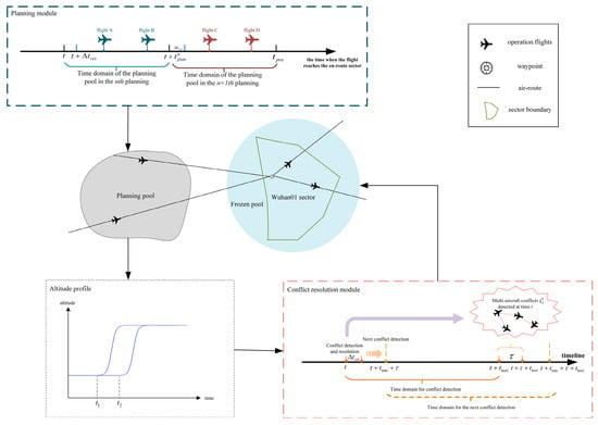
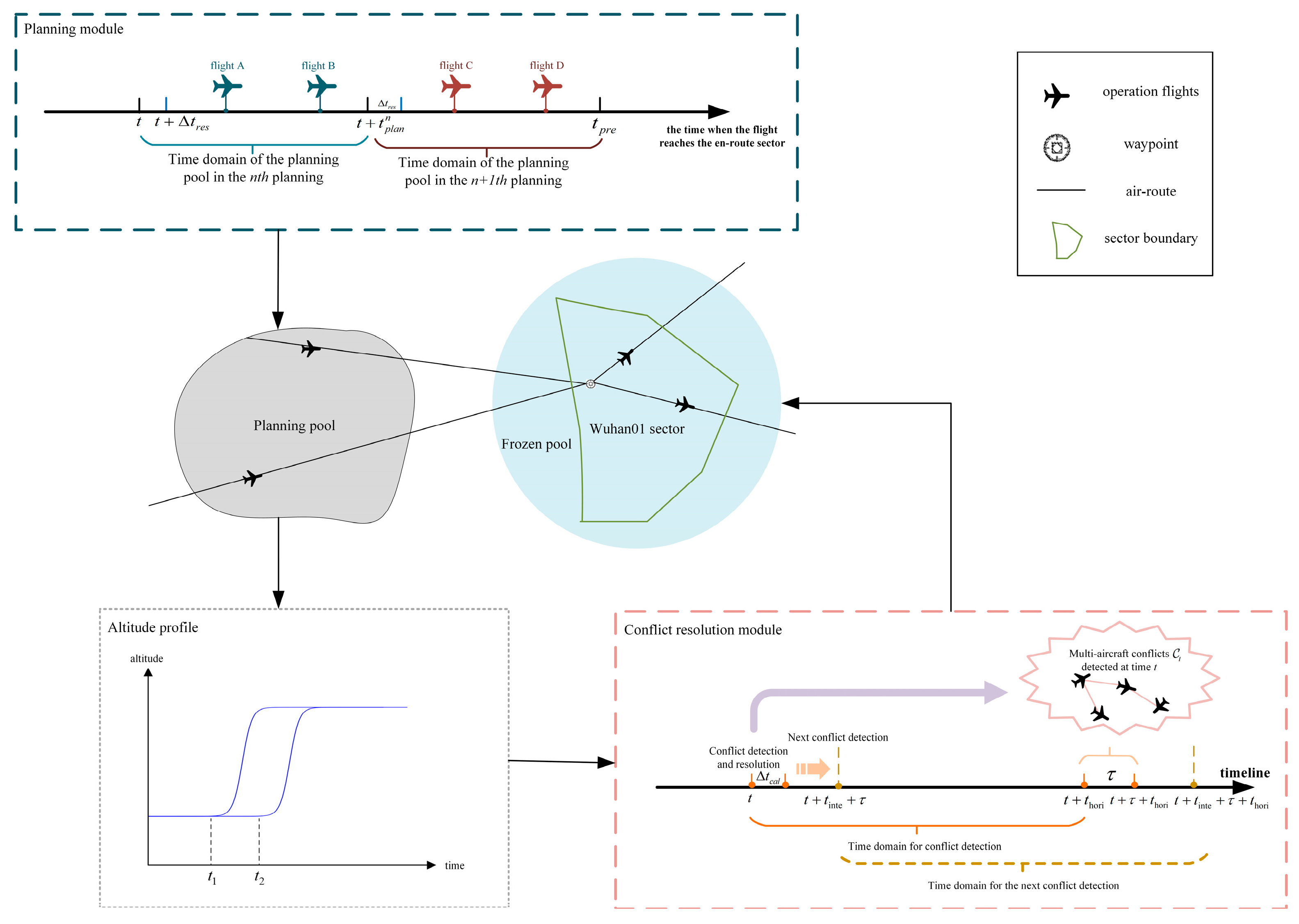
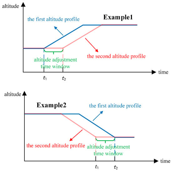
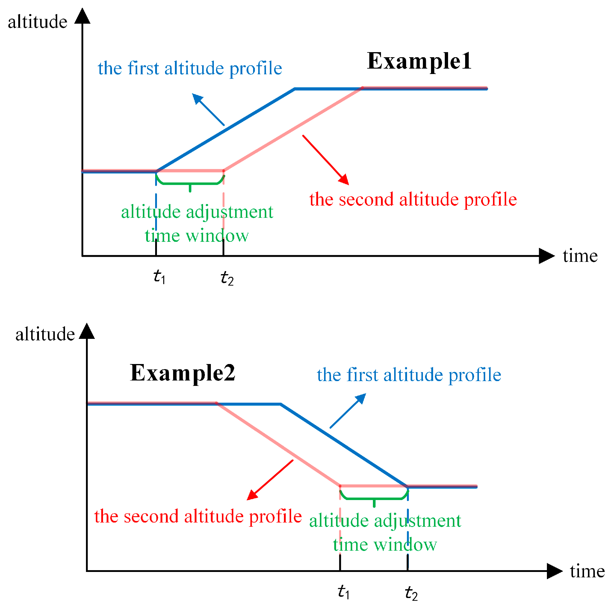
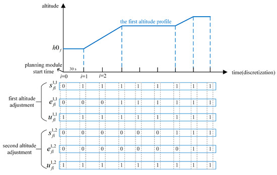
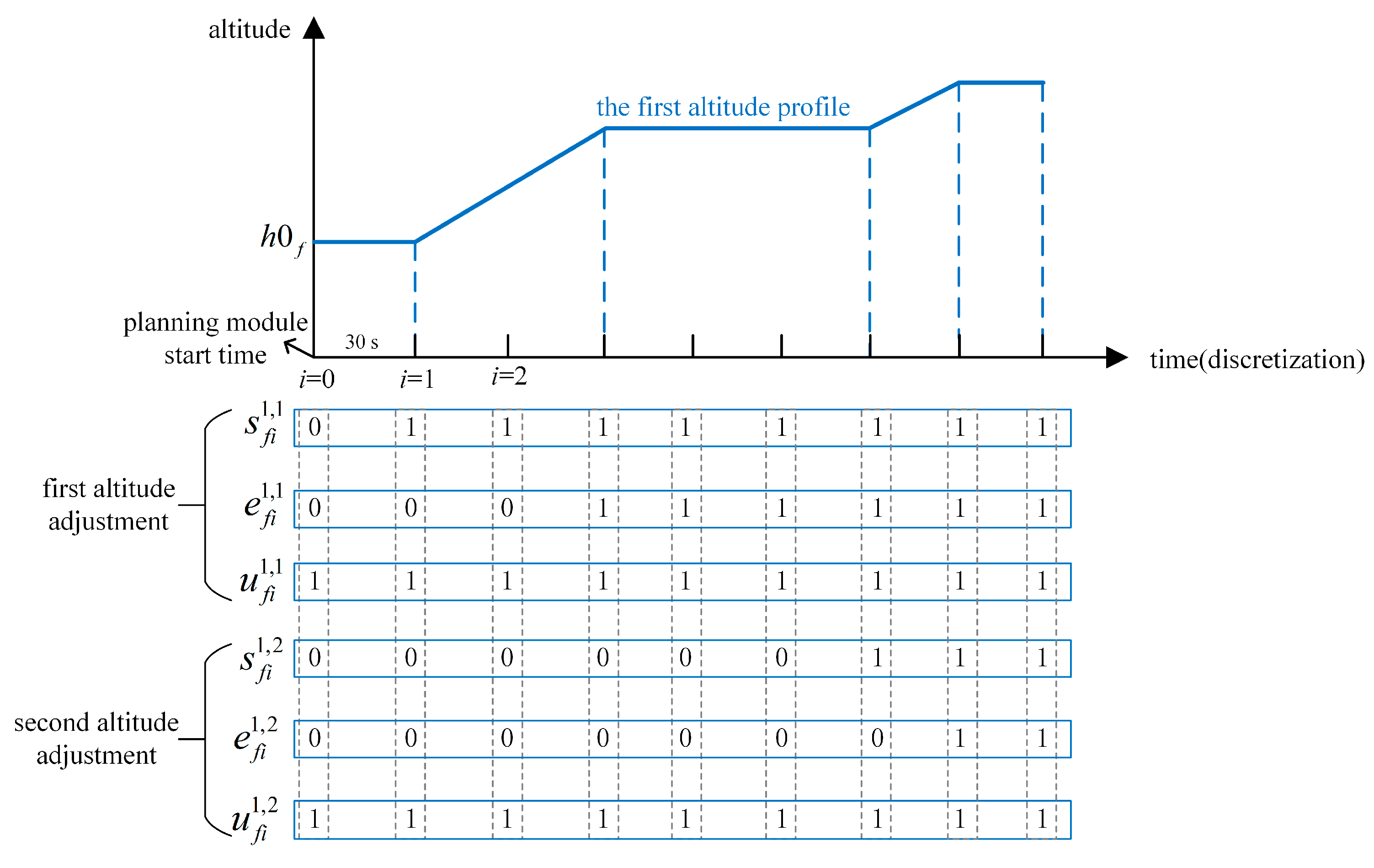
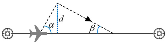
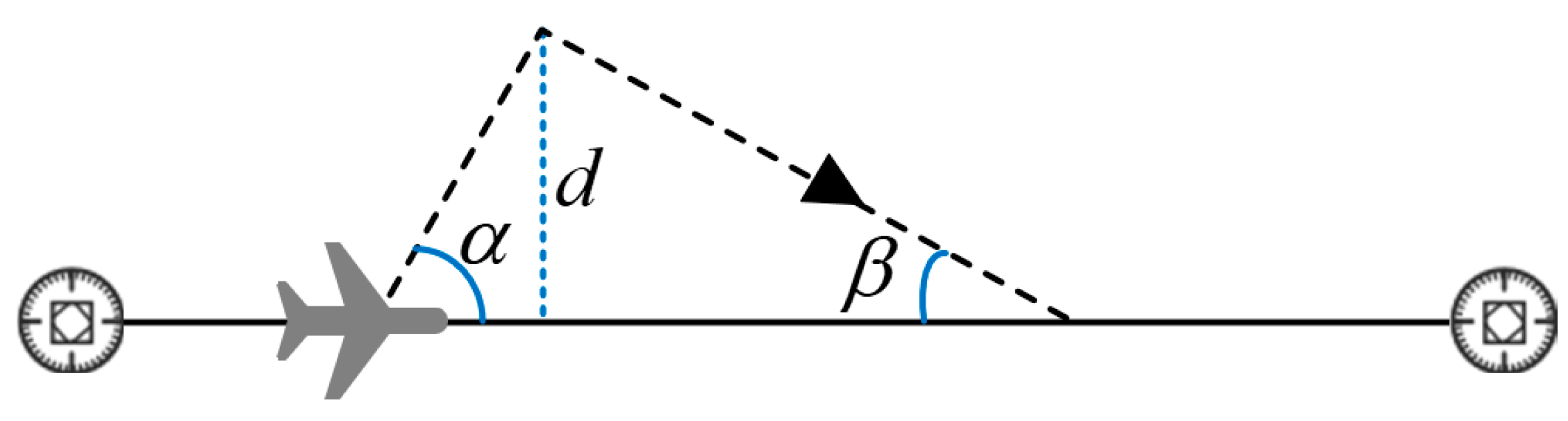
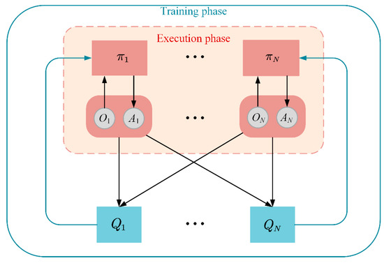
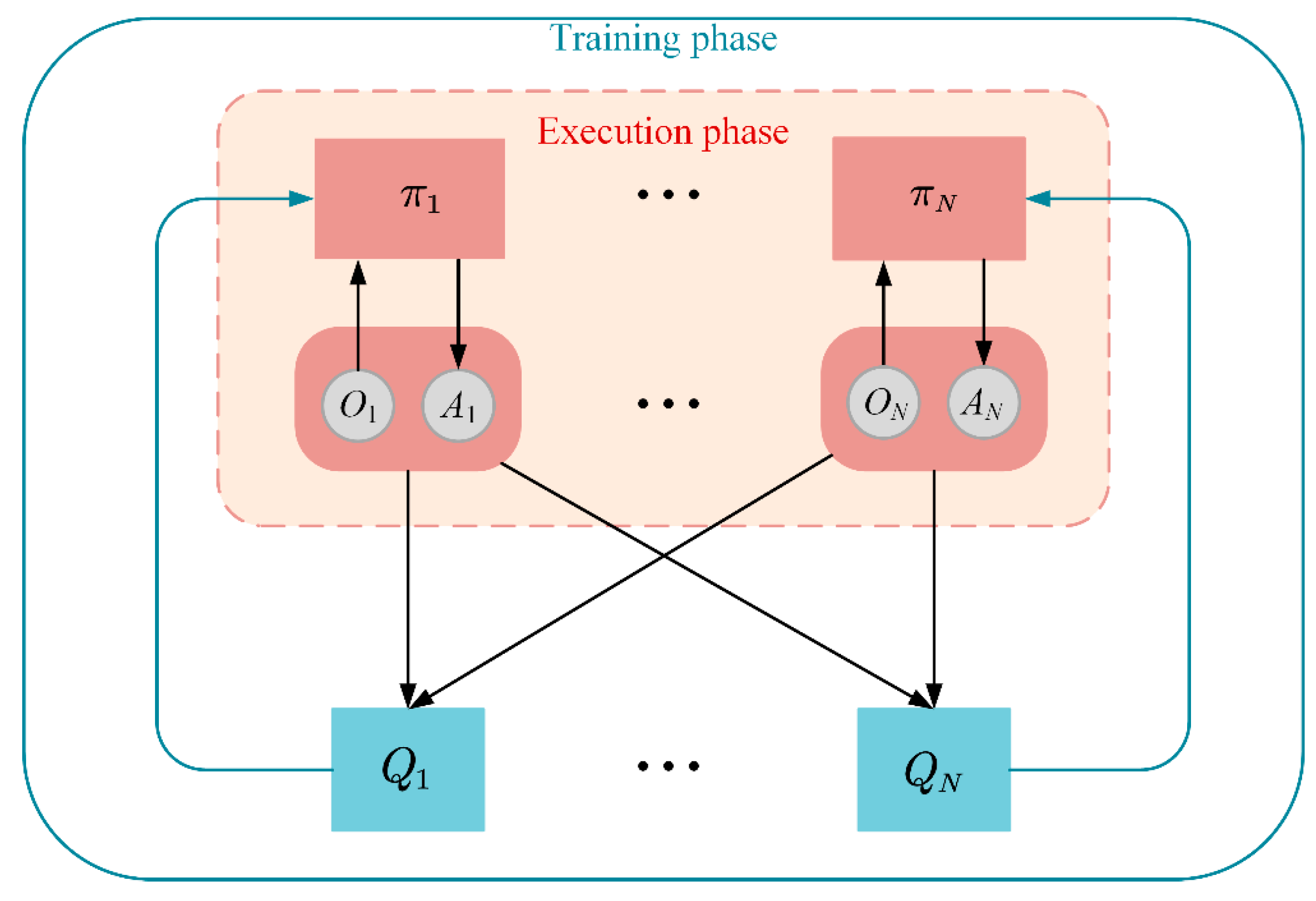
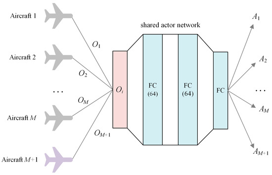
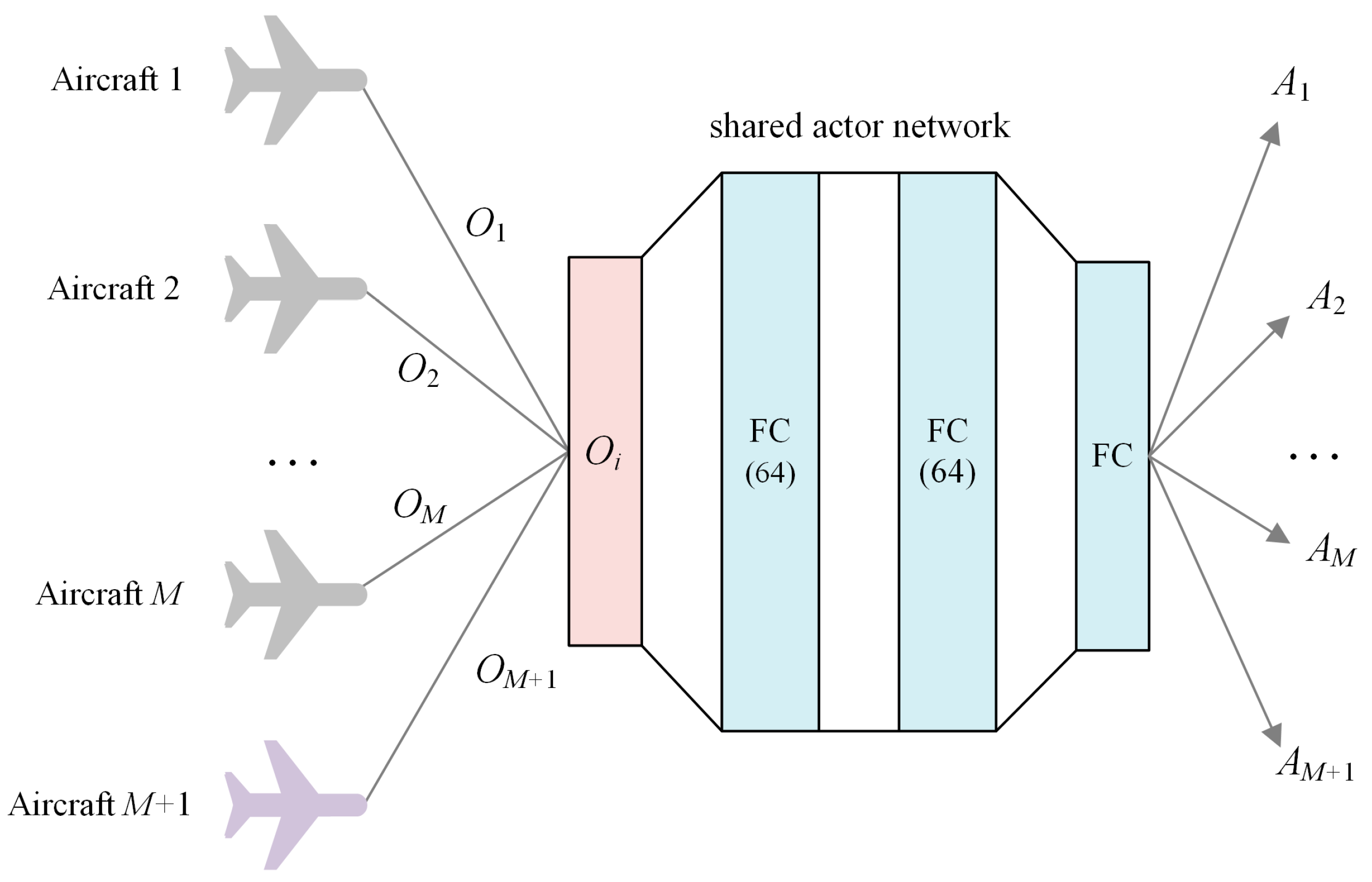
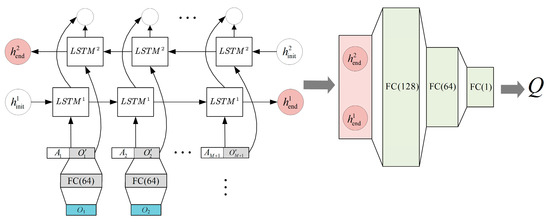
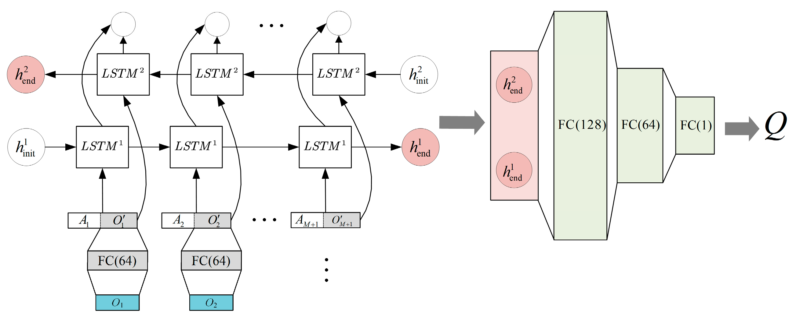
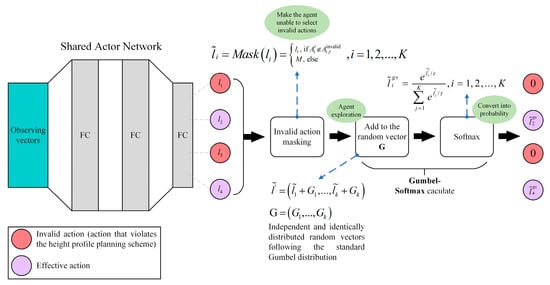
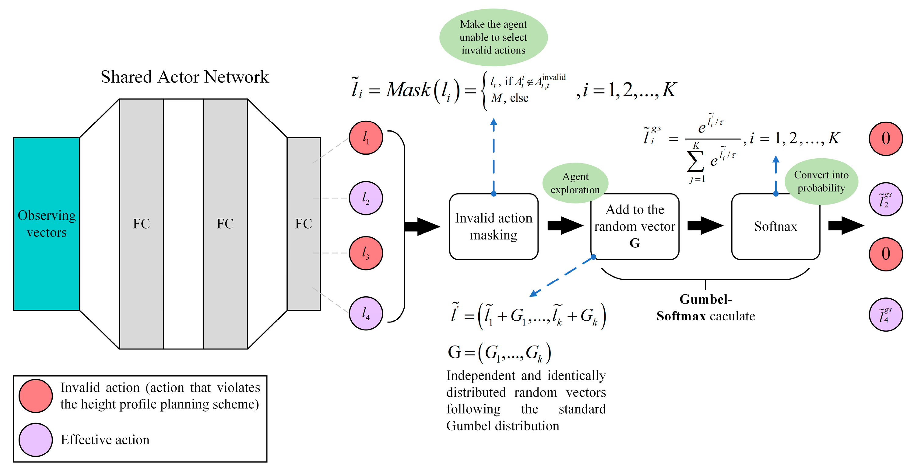
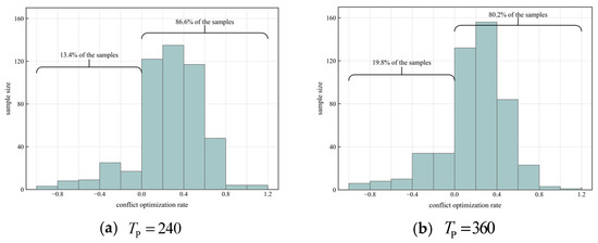
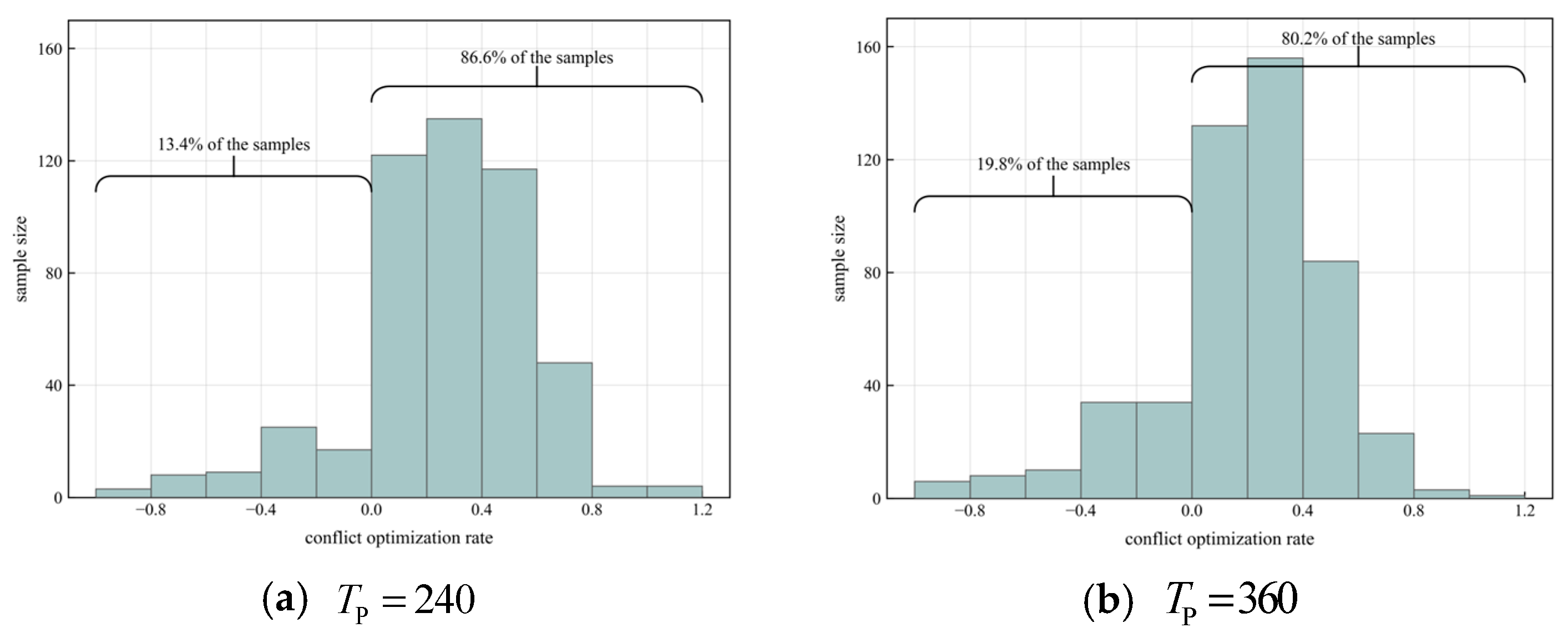
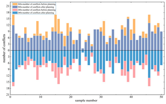
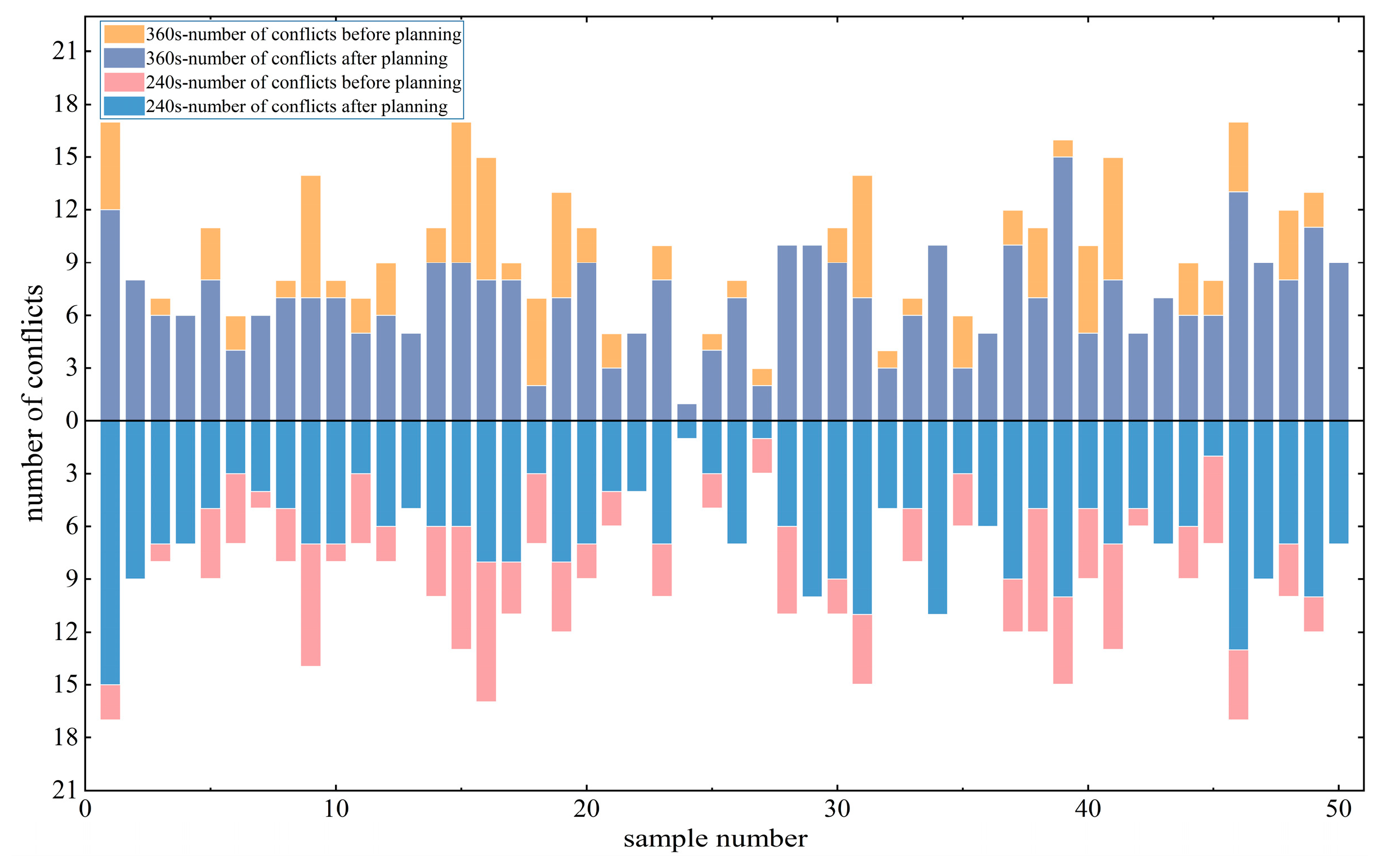
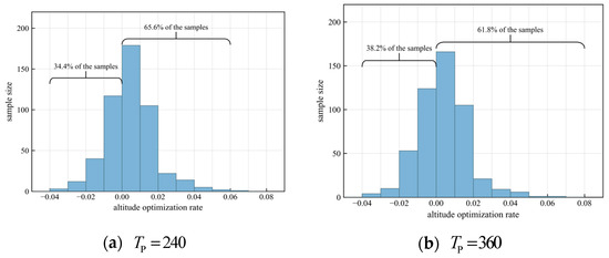
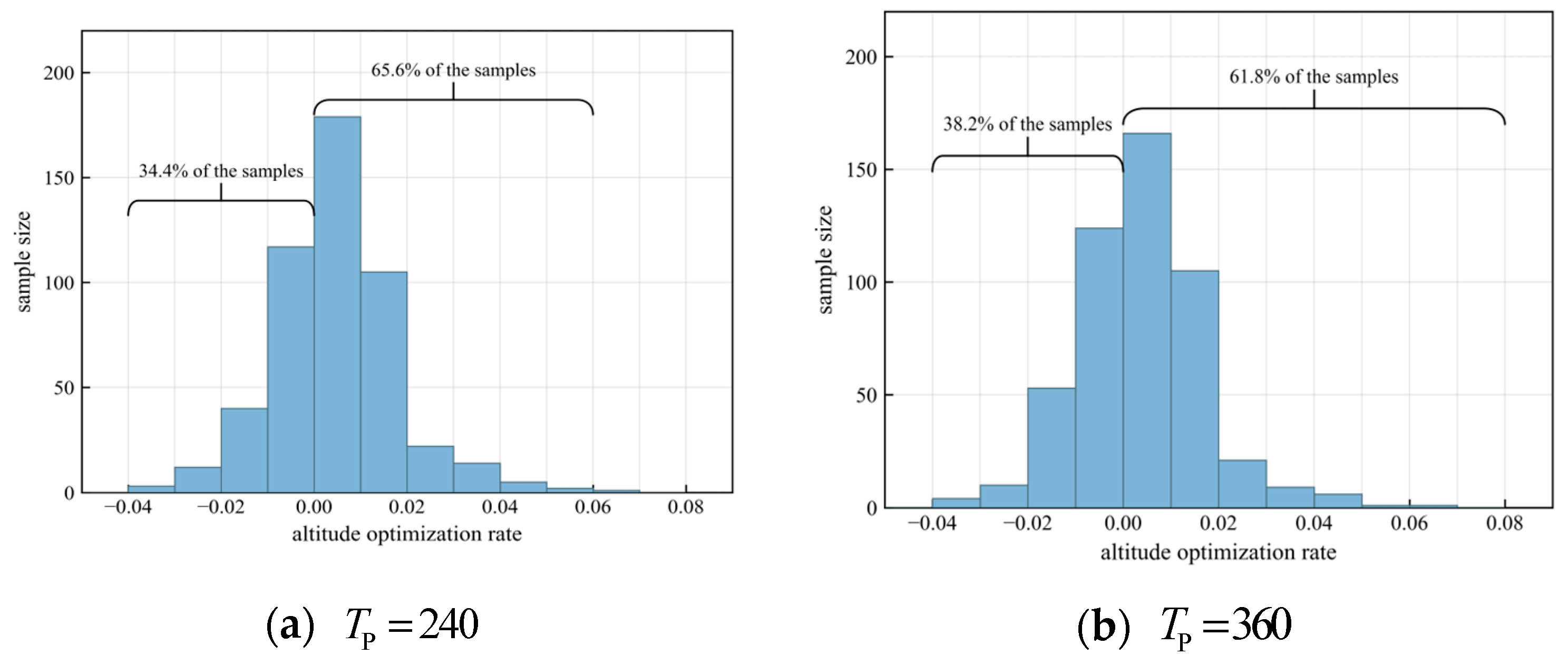
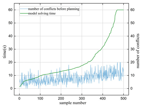
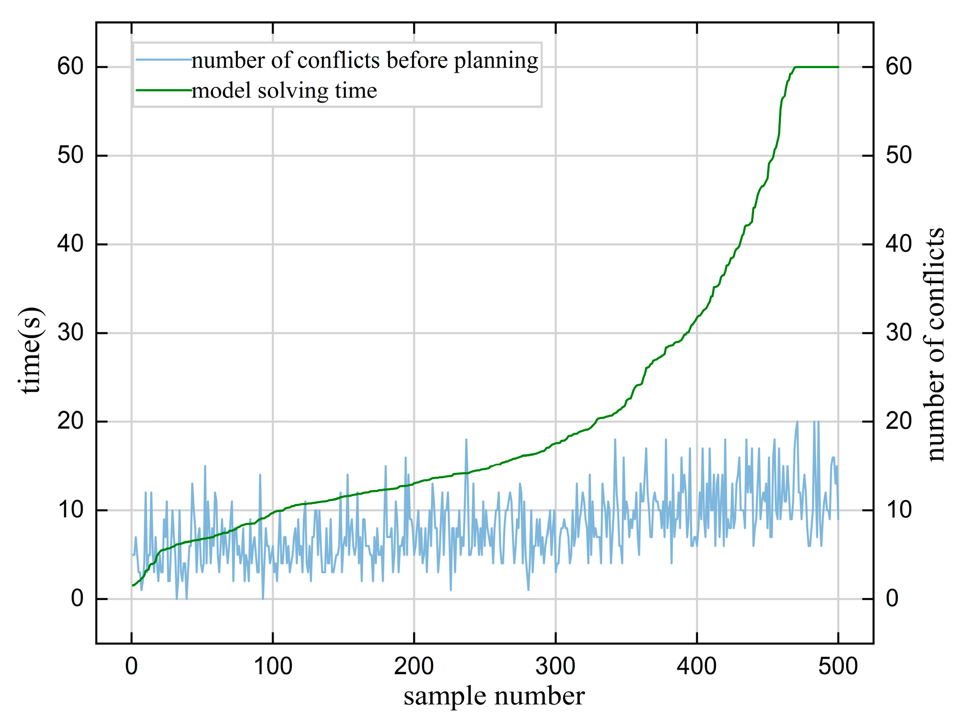
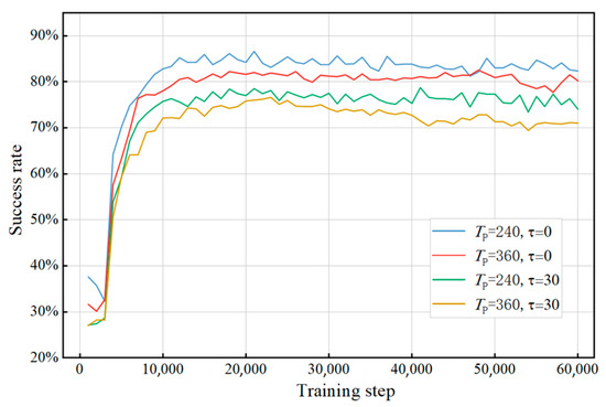
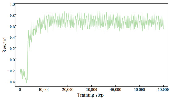
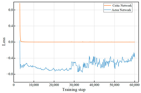
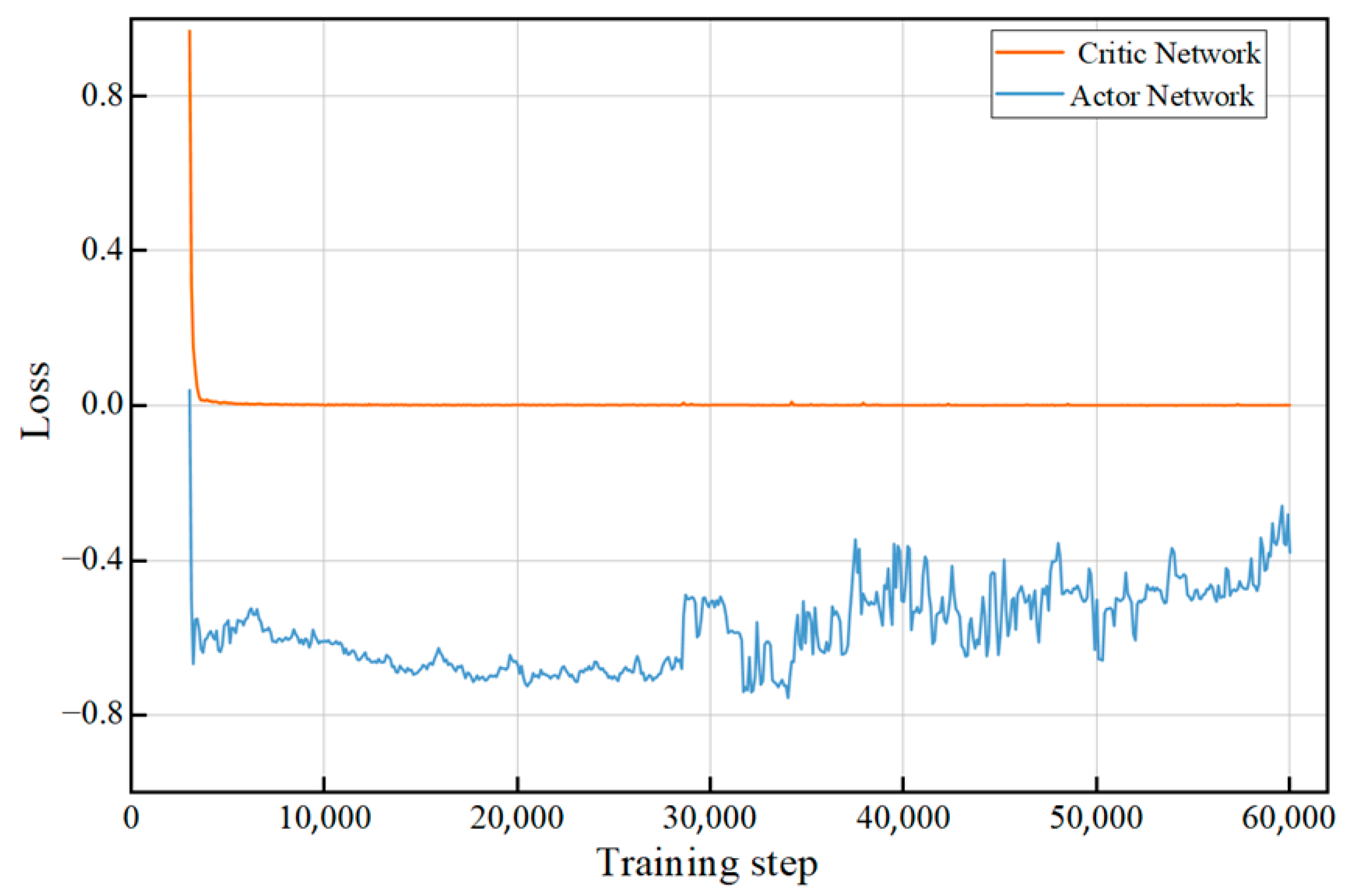
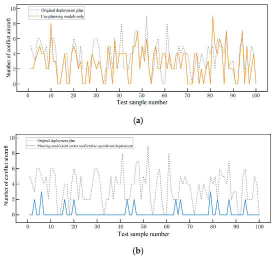
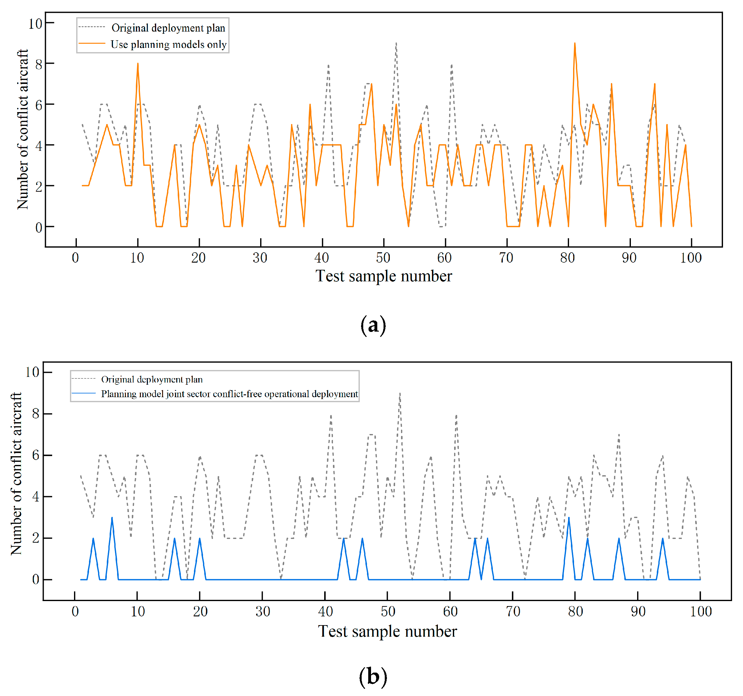
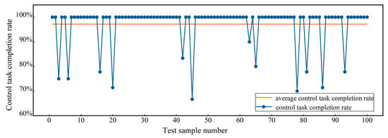
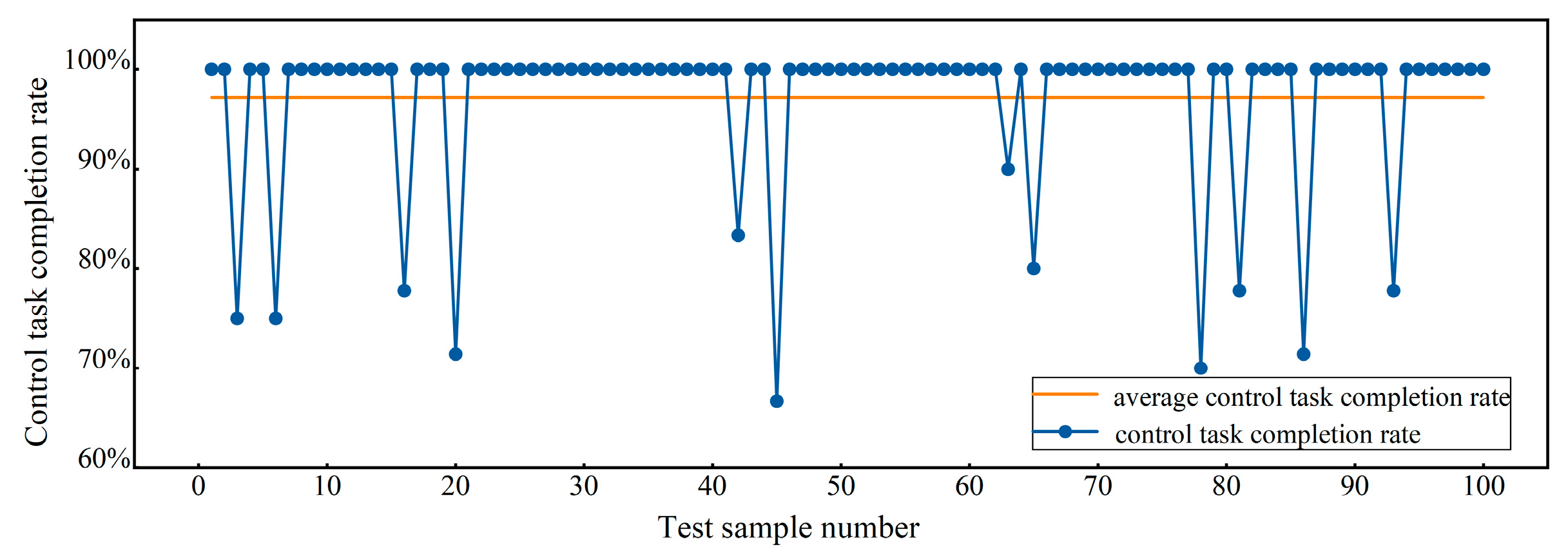

Disclaimer/Publisher’s Note: The statements, opinions and data contained in all publications are solely those of the individual author(s) and contributor(s) and not of MDPI and/or the editor(s). MDPI and/or the editor(s) disclaim responsibility for any injury to people or property resulting from any ideas, methods, instructions or products referred to in the content. |
© 2026 by the authors. Licensee MDPI, Basel, Switzerland. This article is an open access article distributed under the terms and conditions of the Creative Commons Attribution (CC BY) license.