


Abstract
One of the key functions of Air Traffic Management (ATM) is to balance airspace capacity and demand. Despite measures that are taken during the strategic and pre-tactical phases of flight, demand–capacity imbalances still occur in flight, often manifesting as localised regions of high traffic complexity, known as hotspots. These hotspots emerge dynamically, leaving air traffic controllers with limited anticipation time and increased workload. This paper proposes a Machine Learning (ML) framework for the prediction and resolution of hotspots in congested en-route airspace up to an hour in advance. For hotspot prediction, the proposed framework integrates trajectory prediction, spatial clustering, and complexity assessment. The novelty lies in shifting complexity assessment from a sector-level perspective to the level of individual hotspots, whose complexity is quantified using a set of normalised, sector-relative metrics derived from historical data. For hotspot resolution, a Reinforcement Learning (RL) approach, based on Proximal Policy Optimisation (PPO) and a novel neural network architecture, is employed to act on airborne flights. Three single-clearance type agents—a speed agent, a flight-level agent, and a direct routing agent—and a multi-clearance type agent are trained and evaluated on thousands of historical hotspot scenarios. Results demonstrate the suitability of the proposed framework and show that hotspots are strongly seasonal and mainly occur along traffic routes. Furthermore, it is shown that RL agent performance tends to degrade with hotspot complexity in terms of certain performance metrics but remains the same, or even improves, in terms of others. The multi-clearance type agent solves the highest percentage of hotspots; however, the FL agent achieves the best overall performance.
1. Introduction
Air Traffic Management (ATM) plays a crucial role in ensuring the safety and efficiency of air travel. When air traffic demand exceeds airspace capacity, a sector overload occurs and measures need to be taken to restore the balance. These measures include actions by the Network Manager (NM) at the flight planning stage, and Short-Term Air Traffic Flow and Capacity Management (ATFCM) Measures (STAM) implemented by Flow Management Positions (FMPs)—in coordination with the NM—at a later stage (before or during flight) [1]. Such measures are based on predictions—including flight plan data and weather forecasts—and do not consider potential conflicts and traffic complexity within a sector.
During flight, actual conditions may differ from those predicted at the time that the above-mentioned measures are implemented. Aircrafts often end up deviating from their filed flight plan due to convective weather, ground delays, military activity, etc. Such deviations create demand–capacity imbalances and are more likely to create areas of high air traffic complexity—also known as hotspots—that have to be resolved tactically by Air Traffic Control Officers (ATCOs) without sufficient advance notice, resulting in increased controller workload. Even in a sector that is operating within its declared capacity, traffic complexity can vary dynamically in time and space since it depends on many factors—beyond the number of aircrafts that occupy the sector in a given period of time.
Indicators of air traffic complexity can be broadly classified into two categories: static indicators (e.g., airspace factors and operational restrictions) and dynamic indicators (dependent on the traffic situation). Numerous studies have been carried out to model airspace (sector) complexity and identify the best complexity indicators. These are generally data-driven and use a variety of statistical and Machine Learning (ML) techniques and algorithms, including Principal Component Analysis (PCA) and neural networks [2], regression analysis [3], random forest algorithms [4,5], semi-supervised deep learning [6], transfer learning [7], and Hierarchical Graph Representation Learning (HGRL) [8]. Several complexity indicators are identified by these works, such as aircraft count, airspace structure, average vertical speed, number of vertical movements, incoming traffic flows, horizontal proximity, density, and number of potential crossings. Delahaye et al. [9] propose a traffic complexity metric that quantifies the intrinsic complexity of a set of aircraft trajectories by identifying the organisation properties of those trajectories. With this approach, the complexity metric can be computed for each point of a trajectory and represented on a 2D map. Lee et al. [10] model airspace as a closed-loop controlled system responding to disturbances—such as the entry of an aircraft into the airspace—and define complexity in terms of the control activity required to accommodate such disturbances.
Apart from measuring complexity, some works also try to predict complex air traffic events. For instance, Shi-Garrier et al. [11] train an Encoder–Decoder Long Short-Term Memory (LSTM) network to predict traffic complexity up to 40 min in advance. The model is reasonably accurate; however, it is only tested on simulated traffic data. Samardžic et al. [12] propose a methodology for calculating probabilistic complexity—of a sector or airspace—that accounts for prediction uncertainties and includes a weather-related indicator in the calculation. Results show that the error between the probabilistic mean complexity and simulator complexity values is between 12% and 23%. In [13], Moreno et al. train an ensemble model, using random forest algorithms, to predict the complexity of sectors on the basis of flight plan information. Each of the models in the ensemble predicts an operational variable such as clustered flow, entry hour to the sector, medium speed, and number of regulations. Then, the sector complexity is predicted by combining the results of the models. The models are trained and tested with one year of historical data for one sector, and achieve satisfactory results.
Complexity resolution is arguably more complex than detection because it requires an understanding of the consequences of resolution actions, which can be challenging in congested airspace. In the literature, as in ATM operations, complexity resolution is either handled during the pre-tactical phase of flight [14,15,16,17,18]—when aircrafts are still on the ground—or during the tactical phase [19,20]—when aircrafts are already airborne.
In the case of pre-tactical solutions, complexity is generally resolved by delaying departures, rerouting aircrafts, or flight-level capping. For instance, Mannino et al. [14] propose a Mixed Integer Linear Programming (MILP) model to optimally reschedule a set of aircrafts that are forecasted to occupy an overcrowded region of airspace. The model only contains simple combinatorial constraints, corresponding to paths and cycles in an associated disjunctive graph. The model performs very well but was only tested with simulated data. Adacher et al. [15] model the airspace as a directed graph and partition it into sectors, where each sector is controlled by an agent that decides an aircraft schedule to respect delay and capacity constraints. When congestion is predicted, a new aircraft schedule is computed. Two k-shortest path algorithms—a generalised Dijkstra algorithm and a bidirectional search algorithm—are implemented to calculate feasible paths for aircrafts involved in the congestion. The algorithms were tested on simulated data for one sector. Duong et al. [18] present a time-varying queuing network model to apply departure time control and untangle trajectory complexity in hotspot areas. The proposed method successfully reduces up to 45% of potential conflicts with an average delay of 30 min.
Other pre-tactical solutions for hotspot resolution use ML and multi-agent Reinforcement Learning (RL) techniques. Kravaris [16] investigates the use of three collaborative Q-learning methods to resolve hotspots without creating conflicts. Each flight is treated as an agent and the system is tested with simulations based on real-world data. Similarly, Kravaris et al. [17] implement a deep RL method based on the Deep Q-Network (DQN) to resolve demand–capacity imbalances, with thousands of agents representing flights. The measures proposed by the agents are flight-level capping and ground delays. Explanations are provided for agent decisions, and visual analytics methods are used to explore these explanations.
In the case of tactical solutions for complexity resolution, multi-agent RL (MARL) approaches have been attempted in previous work. For instance, Isufaj et al. [19] propose a method to resolve pairwise conflicts (which are considered to be one of the factors that affect complexity) using a multi-agent Deep Deterministic Policy Gradient (DDPG) algorithm, with agent actions limited to heading and speed changes only. The models were evaluated with data from EUROCONTROL’s Demand Data Repository—version 2 (DDR2) [21] and achieve a resolution rate of 93%. In [20], a deep ensemble MARL method is proposed to suggest adjustments to aircrafts in real-time in en-route airspace to avoid air traffic congestion, near-miss situations, and improve arrival timeliness. Only speed actions are allowed and the reward function accounts for conflicts, congestion, delays, and fuel. The method was evaluated with a real-world dataset with thousands of aircrafts.
This work proposes a novel, data-driven methodology to predict and resolve air traffic complexity in en-route airspace, during the tactical phase of flight, up to one hour in advance. Rather than just predicting complexity at a sector level—as is commonly performed in previous work—this work predicts and measures complexity at the level of individual hotspots. Here, a hotspot is defined as a cluster of aircrafts that interact in a complex manner in 4D space (3D position and time). These hotspots are dynamic in nature—evolving in time and space—and their complexity is expressed in terms of multiple metrics. Statistical techniques are used to normalise these metrics on the basis of several years of historical data, and to combine them into a global complexity score per hotspot. This approach results in hotspot complexity values that are relative to the specific sector in which a hotspot is predicted to occur. By computing relative complexity, this approach takes into account the unique characteristics of a sector and can be applied to any sector and any Air Navigation Service Provider (ANSP).
In this work, air traffic complexity is resolved through the application of RL and Proximal Policy Optimisation (PPO). The implementation of the RL agent adopts a unified framework in which a single agent, enabled by a novel neural network architecture, is capable of providing solutions involving multiple aircrafts and clearance types, thereby eliminating the need for coordination among multiple agents. Four different agents are trained: one to generate speed clearances; one to generate flight-level clearances; one to generate direct routing clearances; and one to generate any of the aforementioned clearances. These clearances are applied to one or more airborne flights involved in a hotspot to resolve said hotspot, up to an hour before the predicted time of the hotspot. A multi-objective reward function is implemented to resolve hotspots both safely and efficiently, and a multi-headed policy network is proposed. The agents are trained and evaluated on thousands of historical hotspots.
In practice, any hotspots that are predicted to occur in a sector, and the associated solutions provided by the RL agents, can be presented to the Flow Management Position (FMP) of the Area Control Centre (ACC) that is responsible for that sector. Then, the FMP can coordinate with upstream sectors to implement the suggested solutions. This concept has been validated by the authors [22] and is expected to reduce ATCO workload in the sector where the hotspot is avoided and, consequently, increase airspace capacity and safety.
The rest of this paper is structured as follows. Section 2 describes the hotspot prediction methodology, including data acquisition, trajectory prediction, clustering, and complexity metric calculations. Section 3 discusses the RL-based hotspot resolution process, covering the RL framework, observation and action space, policy network, reward function, and training methodology. Section 4 presents and discusses the results of hotspot prediction and resolution, while Section 5 concludes this paper and provides suggestions for future work.
2. Data-Driven Complex Event Prediction
2.1. Historical Flight Data
The data used for this work are historical data from EUROCONTROL, i.e., the DDR2 dataset [21]. This dataset consists of three types of flight plans:
- M1:
- Flight plans as submitted by airlines.
- M2:
- Regulated flight plans that are the approved flight plans at the time of departure. They include regulation actions taken by the FMP.
- M3:
- The realized flight plans are the ones that represent what was actually flown by the aircraft.
The M1, M2, and M3 datasets are available for 2018, 2019, 2022 and 2023. The years 2020 and 2021 were excluded because traffic was affected by COVID measures. The flight plan information included in this dataset and that is used for trajectory prediction consists of the following:
- Flight metadata:
- –
- Aircraft type.
- –
- Departure airport (ADEP).
- –
- Destination airport (ADES).
- Flight plan data consisting of a list of points:
- –
- Waypoint name: if the point is a known waypoint, the name is provided. Otherwise, a generated name that starts with a special character is provided.
- –
- Position: latitude and longitude.
- –
- Altitude: in feet above sea level.
- –
- Estimate Time Over (ETO): For M1 and M2, the ETO is an estimate. For M3, it is the reported time.
The ETO information is only used for the first point to start the simulation. The trajectory prediction gives a much better time estimate than what is in the original dataset. In addition to flight plans, data are also provided that describe the configuration of the airspace (sectorization). The sectorization data consist of polygons in latitude and longitude space and altitude range that describe the elementary volume of controllable airspace, referred to as the sector.
2.2. Trajectory Prediction
An in-house trajectory prediction algorithm, called SkyTP, predicts the actual trajectory of a flight based on the flight plan (M2). The trajectory consists of the predicted positions and times, as well as the important flight phases such as the top of climb and descent. SkyTP uses physics principles as well as aircraft performance data to make predictions (using an engine based on BADA version 3.16 [23,24]). The use of BADA for aircraft performance is complemented by the use of historical radar data to measure, with better accuracy, some performance parameters. As an example, for each aircraft type, BADA provides a range for the allowable climb and descent rate. However, this range is too wide and the typical values used by the pilots fall within a narrower range. Therefore, this parameter is measured directly from historical data.
The SkyTP model is capable of taking wind and temperature data into consideration if available, with a minor impact on the trajectory prediction resolution when good quality meteorological data are provided. Due to the absence of meteorological data in this work, SkyTP is run under the assumption of no wind and a standard atmospheric model. The impact of this assumption is expected to be smaller than other sources of uncertainty such as the accuracy of the flight plans themselves.
2.3. Clustering
At each time step, the last known position of each aircraft and its flight plan are used to predict its future trajectory, as described previously. For each time step in the predicted future (up to one hour horizon), a clustering algorithm is used to group flights together. The clustering algorithm is geometric and based on the proximity of aircrafts between each other. A tracking algorithm is run to identify the clusters found in the current time step that correspond to those in the previous time step. A hotspot is essentially a cluster that persists over multiple, consecutive time steps and has the following properties:
- An aircraft can only be in one hotspot at a time.
- A hotspot has a start and an end time.
- A hotspot has a position (centroid) and a boundary containing the aircraft. The position and boundary are dynamic, i.e., they evolve in time during the lifetime of the hotspot.
- One or more aircrafts can enter or leave the hotspot during its lifetime.
- A hotspot is characterised by a set of complexity metrics as described above.
2.3.1. Geometric Clustering
The clustering algorithm used is an adaptation of the Density-Based Spatial Clustering of Applications with Noise (DBSCAN) clustering algorithm [25]. DBSCAN is based on the notion of local density and the notion of chained connectivity (illustrated in Figure 1). It requires one input parameter representing the size of a neighborhood. The DBSCAN algorithm does not require the knowledge of the number of clusters in advance and has a built-in outlier detection allowing points to not belong to any cluster. The distance metric used for density calculation is customizable. For this work, we use the 2D haversine distance between aircrafts, with a threshold on the vertical separation of 1000 feet:
Figure 1.
DBSCAN: chained connectivity. Two points are connected if they are reachable from the same point.
Swiss ATCOs receive a notification of a potential conflict when the separation between two aircrafts is less than 15 NM horizontally and 1000 feet vertically. According to this definition, we consider that aircrafts with higher separation than these thresholds do not induce additional workloads to the ATCOs and therefore should not be clustered together. For the DBSCAN algorithm, we have therefore chosen a neighborhood size of 15 NM and a distance metric that takes into account the vertical separation.
2.3.2. Time Tracking of a Hotspot
Two clusters detected in two consecutive time steps are considered the same if at least half of the contributing aircrafts are the same. Matching of two clusters with fewer than half of the aircrafts is allowed if the matching is unambiguous, i.e., it is a one-to-one matching. With this definition, hotspots are allowed to split or merge during their evolution (Figure 2).
Figure 2.
Time tracking of geometrical clusters to form dynamic hotspots.
2.4. Complexity Metric Calculation
Historically, the FMP works with a single metric to assess the complexity of a sector, namely the sector occupancy. In contrast, in this work, several complexity metrics are defined. The metrics are defined for a single time snapshot, which means the complexity of the hotspot is dynamic and evolves during its lifetime. To describe the complexity of the hotspot as a whole, we use the mean complexity over the duration of the event.
2.4.1. List of Metrics
Below is a list of the metrics implemented for this work:
- Number of aircrafts:
- –
- : the number of aircrafts in the sector.
- –
- : Density; number of aircrafts in the cluster divided by the size of the cluster, i.e., the area of the smallest convex polygon enclosing the cluster.
- Conflicts (see Section 2.4.3):
- –
- : Number of Medium-Term Conflict Alerts (MTCAs): pairs of aircrafts that are predicted to lose a separation of 5.5 NM within 2.5 min from the prediction time.
- –
- : Number of Long-Term Conflict Alerts (LTCAs): pairs of aircrafts that are predicted to lose a separation of 7.9 NM within 15 min from the prediction time. This number excludes the MTCAs.
- –
- : A weight that depends on the distance of closest approach of the aircraft in conflict .
- –
- : A weight that depends on the time to the point where the distance of closest approach between two aircrafts in conflict occurs .
- –
- : A weight that depends on both and .
- Proximity to sector boundaries (see Section 2.4.4):
- –
- : Number of aircrafts weighted according to their horizontal distance from the sector centroid.
- –
- : Number of aircrafts weighted according to their vertical proximity to sector boundary.
- Dynamic aircraft:
- –
- : Number of aircrafts in climb phase.
- –
- : Number of aircrafts in descent phase.
- –
- : The standard deviations of the heading of the aircraft in the hotspot. This metric helps give different complexities to situations where a group of aircrafts follow the same heading on a common route, and situations where routes intersect each other in a more complex configuration.
- –
- : A metric dependent on the presence of aircrafts that have a non-standard vertical profile. It is defined in (Section 2.4.5).
- Miscellaneous:
- –
- : Number of different aircraft categories (see Section 2.4.6).
- –
- : The complexity of the sector in which the hotspot occurs. The sector complexity is computed using the metrics above and considering the flights within the sector as a single cluster.
The thresholds used for the MTCA and LTCA definitions above correspond to the operational definitions from the Conflict Detection Tool (CDT) used by the Swiss ATCOs.
2.4.2. The Complexity Unit
To have a unique complexity unit among the different complexity metrics, each metric is scaled into the range [0, 100] such that the complexity is expressed as a percentage. The scaling is learned from a reference dataset taken from the historical data. With this scaling, an intuitive interpretation of the complexity is provided. For instance, a complexity of 90 means that 90% of the situations encountered in the reference dataset have lower complexity.
The reference dataset for calibrating the complexity metrics consists of the equivalent of one year of data selected randomly across the full dataset. We selected the time range during busy hours between 8:00 AM and 8:00 PM, excluding low traffic times to avoid the bias of over-populating the very low complexity regime. Each airspace was calibrated independently, introducing the notion of “relative complexity”. This would account for the fact that in an airspace where the ATCO is equipped with automation tools (e.g., automated conflict detection), the same traffic seems less complex compared to an airspace where ATCOs do not have the same tools at their disposal.
The different complexity metrics are combined into a global complexity using a statistical model. First, the complexity metrics are decorrelated using PCA [26] and then combined as independent variables by taking the quadratic average:
With this definition, the hypersurfaces of constant complexity lay on hyperspheres in the complexity hyperspace (in two dimensions, defines an arc of a circle for and ).
2.4.3. Conflict Complexity
A conflict is the prediction of the potential loss of separation of two aircrafts. It is characterized by two parameters:
- : expected distance of closest approach between two aircrafts.
- : time at which the distance of closest approach is expected to happen relative to the time when the prediction is being made.
According to the conventions used in operation, we are interested in two types of conflicts:
- MTCA: < 5.5 NM and < 2.5 min.
- LTCA: < 7.9 NM and < 15 min.
The complexity metrics associated with conflicts can be computed either from the number of conflicts in the above categories, or from the continuous parameters and .
Three complexity metrics are defined:
- : a 1D weight based only on .
- : a 1D weight based only on .
- : a 2D weight based on both and .
The 1D weights are defined as inversely proportional to the corresponding variable, and take the value of 1 at the transition between MTCA and LTCA. The 2D weight is defined using this formula:
where n is an exponent that can be adjusted to change the weight distribution. With this definition, for large values of n, the lines of equal weights approximate rectangles in the 2D space. We used the value of for this implementation. All weights are then capped at a maximum value of 10. Figure 3 shows the weights for the three metrics.
Figure 3.
Definition of the complexity metrics associated with conflicts (Dashed lines correspond to the boundary between an MTCA and an LTCA).
2.4.4. Proximity to Sector Boundaries
Horizontal proximity to sector boundaries :
Computing the exact distance to the nearest sector boundary is expensive. We can use an approximation to speed up the computation. The distance to the sector boundary can be approximated by the following procedure:
- Centroid of the sector: we compute the average position of all points on the polygon defining the sector boundaries.
- Effective radius of the sector: we compute the average distance between points on the sector boundary to the centroid of the sector.
- Relative distance: for each aircraft in the hotspot, we compute the relative distance to the centroid of the sector, which is the distance divided by the effective radius.
- Weight: we apply a weight based on the ratio between the distance to the centroid and the effective radius, representing the probability of being outside the polygon.
Determining the weight function:
The objective of the weight function is to provide a smooth transition between the sector’s interior and exterior when crossing the boundary. The chosen weight function is defined as the probability of being outside the sector given the distance to the centroid.
To determine the weight function numerically, a toy simulation was performed as follows: We generate random polygons. For each generated polygon, we generate uniformly distributed random points and compute their relative distance to the centroid of the polygon. We then find the fraction of points outside the sector as a function of the relative distance to the centroid. We noticed that the obtained curve can be fitted with a good quality fit with a gaussian cumulative distribution function (CDF). Figure 4 shows the curve that defines the weight as a function of the relative distance (left) and overlayed on the Geneva sector boundary as an example (right).
Figure 4.
Left: The weight as function of the relative distance, with the gaussian fit ovelayed. Right: the weight overlayed on the geometry of the Geneva upper airspace sectors.
Vertical proximity to sector boundaries :
On the vertical axis, the computation is less expensive because sectors are cylinders and the vertical span is defined by minimum and maximum flight levels. We can explicitly compute the vertical distance to the mid-level and normalize it by half the vertical size of the sector. The weight function is therefore a simple linear function that goes from 0 to 1 between the mid-level and the sector boundary, as shown in Figure 5.
Figure 5.
The weight (horizontal axis) as a function of the vertical position within the sector (vertical axis).
2.4.5. YOYO Complexity
To define the YOYO complexity, we assign a YOYO score to each flight in the hotspot. This score is based on the flight plan of the aircraft inside the sector where the hotspot occurs. The YOYO score counts the number of transitions between the three phases of flight: climb, cruise, and descent. An extra bonus point is given if the aircraft enters the sector in an already evolving state (climb or descent). Figure 6 shows a few examples of vertical flight profiles (expected altitude vs. time) and the corresponding YOYO score. The vertical lines show the transitions; the ones that have an extra bonus point are shown in red, and the others are shown in green. The YOYO complexity of the hotspot is the average YOYO score on the flights in the hotspot.
Figure 6.
Examples illustrating the YOYO complexity definition.
2.4.6. Number of Aircraft Categories
To define the number of aircraft categories, we group the aircraft types into classes of similar properties. This grouping is based on BADA data, which characterize each aircraft type by a total of 165 performance parameters, including aerodynamic coefficients, thrust and fuel-flow models, mass characteristics, speed schedules, and operational limits. We ran a clustering algorithm on the full set of aircraft features available in BADA. We found that the different aircraft types can be grouped into seven categories. Figure 7 shows the clustering result as a function of the 2D distributions of the highest PCA components describing the BADA dataset and Figure 8 shows the same result as a function of the mass and the engine type of the aircraft. We found that the mass of the aircraft and the engine type highly correlate with the discovered classification.
Figure 7.
Scatter plot of the two highest PCA components describing the BADA dataset. Each cluster is represented in a different color. We show, for each cluster, the centroid position as well as the ellipse that represents the spread for that cluster.
Figure 8.
Scatter plot of the average aircraft mass vs. the engine type for each aircraft category. The error bars represent the spread for each cluster.
3. Complex Event Resolution
3.1. Role of the RL Agent
Once a hotspot is predicted, the resolution module is activated to find a viable dissipation strategy. This module is designed as a sequential decision-making process where the goal is to recommend a series of minimally invasive tactical clearances. An ML-based solution using neural networks was considered appropriate due to the complex nature of resolving hotspots. Implementing such a solution requires training of the neural networks and, given the absence of ground-truth labelled data—to indicate what actions are normally taken by ATCOs to resolve hotspots—the problem was formulated using an RL approach. RL allows an agent to learn effective control policies through trial-and-error interaction with a simulated environment, making it ideal for this application, as it can reveal previously unknown dissipation solutions. Following the training phase within the simulated environment, the weights of the RL agent are fixed and thus can be applied to provide clearances in an operational setting.
3.2. RL Framework
The hotspot resolution process is modelled using a standard agent–environment framework, as depicted in Figure 9. The environment is responsible for managing the airspace simulation, which leverages the SkyTP trajectory predictor to model the evolution of flight paths based on agent-issued clearances. At each time step, the environment provides the agent with an observation of the current state of the simulated sky and a scalar reward signal. The agent, which is a policy network trained using a PPO algorithm, receives this information and outputs an action. This action is processed into an Air Traffic Control (ATC) clearance, which is then fed back into the simulation, creating a closed loop that continues until the hotspot is either resolved or the episode exceeds the time limit of 64 time steps (equivalent to an hour), which terminates the episode.
Figure 9.
Overview of the RL hotspot resolution framework.
The previously described interaction with the simulation environment is used not only to train the RL agent but also in an operational setting. In the operational setting, the agent’s direct output is initially executed during a simulated episode. Following this, these outputs are concatenated to construct the final clearances for real-time application.
3.3. Observation Space
The observation space defines input variables that provide information to the agent at each step to make a decision. These variables were chosen with the aim of providing the agent with the necessary information to comprehend the current sky and decide how to resolve a hotspot. Therefore, the observation space includes a combination of variables on the hotspot and its surrounding traffic context. The input variables are obtained from SkyTP for 20 aircrafts and are organized into three main categories:
- Resolution Aircraft: A fixed-size vector for up to six primary aircrafts directly involved in the hotspot, which represents the aircraft on which the RL agent can act. The resolution window of six aircrafts was chosen because it represents the median number of flights involved in a hotspot, as identified from the historical training dataset, providing a representative but computationally manageable input size. The six aircrafts are ordered by complexity and, for these aircrafts, the state variables include the current position; speed; heading; aircraft mass; the next five planned waypoints; the remaining number of waypoints until the entry point of the sector in which the hotspot would occur; and a metric representing each flight’s contribution to the complexity of the hotspot. The resulting vector size is .
- Context Aircraft: To provide wider situational awareness, the state includes information on 14 additional flights—flights that are directly involved in a hotspot but do not fit the resolution window, and other flights whose lateral profiles are predicted to intersect with any of the primary hotspot aircraft lateral profiles. The flights in this category are described by a smaller set of variables, compared to the previous category, to reduce the dimensionality of the observation space. The variables for these flights exclude metrics, such as aircraft mass, which are not directly under the control of the agent and therefore less relevant for context. The resulting vector size is .
- Global Context: Additional variables are included to provide information that is relevant to all flights in the observation space and to provide temporal context. The overall hotspot complexity is included to allow the agent to relate it to the complexity reduction reward, the most important factor in the reward function and the main goal of the proposed solution. For temporal context, the 10 most recent clearances issued by the agent are included (their value, start time, and duration), which also serves as context on the validity of previously issued clearances. In addition, a time-based variable is included to indicate the progress of the episode. The resulting vector size is .
The position of the variables in the input vector for the aircraft was kept constant, i.e., the first six aircrafts would be at the start, followed by the fourteen crossing flights and the additional variables. Padding is used to ensure this position for hotspots with fewer flights. This results in a constant vector size of . The observations are normalised according to minimum and maximum values gathered from historical flight track data for 2018. This normalisation was preferred over rolling normalisation due to limitations in the speed of the simulation environment.
3.4. Action Space
The agent’s action space is a composite structure designed to form a complete ATC clearance. At each step, the agent outputs a tuple consisting of aircraft choice, clearance type, and clearance value. This allows the agent to issue one clearance to one aircraft per decision step. Separate agents were trained, each specializing in a single clearance type:
- Speed changes;
- Flight-level changes;
- Direct routing.
The clearance type is a categorical output indicating whether to apply the clearance or to perform a “no-operation” (no-op), which means that the agent will wait one time step without changing the sky. The clearance value is a continuous output in the range [−1, 1]—which represents a change from the aircraft’s current value—that is subsequently denormalized and processed. For direct routing, this continuous dimension is discretized to represent the direct routing option. For speed changes, the clearance value is denormalized by 0.01, resulting in possible Mach changes between −0.01 and 0.01 per episode step.
To ensure operational feasibility, action masking is applied to constrain the agent’s actions. These restrictions, set by domain knowledge, are enforced by ignoring invalid actions; this knowledge implicitly controls the RL agent’s exploration to avoid them. Key constraints include the following:
- Speed clearances are only issued to aircrafts that have reached their cruise flight level. This was performed because it was observed that aircrafts do not always manage to adjust their speed according to the clearance if that clearance is issued during a climb or descent. This approach is also in line with current ATC operations.
- Flight-level clearances are restricted to the climb and descent of a flight, and such clearances are only allowed in the same direction (i.e., climb and descend instructions are only issued to climbing and descending aircraft, respectively). This restriction mitigates multiple changes in climb and descent.
- Direct routing clearances are always given directly to the planned entry point of the sector where the hotspot would occur. This was partly performed to simplify the implementation of the direct routing agent and so as not to change the entry conditions of an aircraft in the sector of interest.
- Clearance values are clipped to operationally acceptable ranges: requested flight levels are limited to the range between FL320 and FL390, and airspeed is limited to the range between 0.7 and 0.82 Mach. These ranges were chosen to allow the agent to output clearances close to potential solutions from the start of training.
3.5. Policy Network
To accommodate the composite action space, a multi-headed policy network is implemented as shown in Figure 10. This architecture allows for dependent decision-making, where the choice of clearance type is conditioned by the aircraft choice, and the clearance value is conditioned by both aircraft and clearance type choice. The network consists of the following:
Figure 10.
Architecture of the policy network. Note that is the observable from the environment and the action is comprised of the tuple (ACFT#, CLR type, CLR value).
- Shared Body: An input layer followed by a combination of LSTM and fully connected layers that process the observation and extract a shared set of features relevant for all decisions.
- Output Head 1 (Aircraft Choice): Takes the shared features as input and outputs a categorical distribution over the six possible aircraft to act upon.
- Output Head 2 (Clearance Type): Takes the shared features and the aircraft choice from Head 1 as input. It outputs a categorical choice between implementing a clearance or a no-op.
- Output Head 3 (Clearance Value): Takes the shared features, aircraft choice (Head 1), and clearance type (Head 2) as input to produce a continuous value to be processed as a magnitude for the chosen clearance type.
This dependent structure ensures that the agent’s full action is cohesive, improving its learning stability and functionality.
3.6. Reward Function
The reward function guides the agent’s learning process by providing feedback on its actions during the training phase. A multi-objective negative reward function is used to encourage the agent to resolve the hotspot as safely and efficiently as possible. A hotspot is considered solved if, after a solution is applied, it is no longer detected by the prediction module described in Section 2. At each time step, the total reward is a weighted sum of six components as shown in (4):
The components, in order of descending priority set by their corresponding weight w, are as follows:
- Primary Objective (): The core reward is based on the reduction in the target hotspot’s complexity. A large positive reward is given if the hotspot is solved completely.
- Secondary Objectives (, ): Penalties are issued for creating new hotspots or new conflicts elsewhere in the airspace. This is performed to prevent domino effects.
- Tertiary Objectives (): The negative reward structure inherently discourages excessive clearances. To encourage focused solutions, an additional penalty is applied based on the number of unique aircrafts that are given clearances.
- Quaternary Objectives (, ): Small penalties are applied for increasing fuel consumption or a significant lateral deviation from the original flight plan, encouraging efficient and minimally disruptive solutions.
The weights were selected empirically to reflect the priority of different objectives based on discussions with operational experts and to ensure balance between different standardizations of reward components. The weights were set to the following values: .
3.7. Training Methodology
The training process for the RL agent was structured to incrementally increase the environment complexity by evaluating individual clearance types before combining them into a comprehensive strategy. The training scenarios were derived from a historical dataset of hotspots (previously described in Section 2.1), to ensure that the agent learns from realistic traffic scenarios. For all experiments, the agent’s observation was configured with a resolution window of six aircrafts and fourteen additional aircrafts, as described in Section 3.3. To enhance diversity during training, the observations of all aircrafts were shuffled. This ensured that the RL agent would observe episodes with different aircrafts in the case of more than six directly involved flights or more than fourteen crossing flights.
3.7.1. Single-Clearance Type Agent
To establish a performance baseline and analyse the isolated impact of each tactical clearance type, three specialised agents were trained first. Each agent was restricted to a simplified action space, capable of issuing either a no-operation (NOOP) command or a single type of clearance:
- NOOP + Flight Level (FL): An agent focused exclusively on vertical adjustment resolutions.
- NOOP + Speed (SPD): An agent focused exclusively on speed adjustment resolutions.
- NOOP + Direct-to (DCT): An agent focused exclusively on re-routing adjustments via direct-to-waypoint clearances.
This approach allows for a clear attribution of performance changes to a specific resolution strategy. The training time was equal for each single clearance type agent, where the best agent was chosen from training for approximately 48 h using 90,000 time steps for optimisation.
3.7.2. Multi-Clearance Type Agent
Following the evaluation of the single-clearance type agents, a comprehensive multi-clearance type agent was trained on the same historical dataset as that used for the single-clearance type agents. This agent operates on the full, composite action space described in Section 3.4, enabling it to select the most appropriate aircraft, clearance type (FL, SPD, or DCT), and clearance value in a single decision step. This configuration represents a more operationally realistic model, where the agent must learn the synergistic or competing effects of different resolution types to find an optimal strategy. The training for this agent was longer compared to the single-clearance type agents due to the significant increase in action possibilities. The samples used for each update were doubled, resulting in a training of approximately 4 days and 180,000 time steps used for optimisation.
The hyperparameters used to train the agents are summarized in Table 1.
Table 1.
Hyperparameters for training the single- and multi- clearance type agents.
3.7.3. Hotspot Scenarios for Training and Evaluation
The training dataset was populated with historical hotspot scenarios identified from the dataset described in Section 2.1. The hotspot scenarios were selected by hotspot complexity, resulting in five equally sized complexity bins—with 600 hotspots per bin—corresponding to complexity values between 0.5 and 1.0. The hotspots were selected by randomly sampling over the four years of data during peak hours (between 8 am and 8 pm), while making sure that each hotspot was detected at least 30 min before its start, and that there was no repetition of hour–date–year combinations to ensure variety. Hotspots with a complexity value below 0.5 were classified as nominal traffic, thereby establishing a minimum complexity threshold of 0.5 for the dataset.
Figure 11 and Figure 12 show distributions of key hotspot attributes and the hotspot locations on a 2D map, respectively. These visualisations provide a comprehensive overview of the data landscape in which the RL framework was trained and evaluated. The top plot in Figure 11 shows the delay between hotspot detection and the start time of a hotspot, where most hotspots were detected between 30 and 60 min before they were predicted to occur. The middle plot illustrates the distribution of hotspots across the complexity bins, with the highest complexity reaching approximately 0.95. The bottom plot provides the number of flights involved in each hotspot, showing that only a few cases involved hotspots with a large number of flights. As explained in Section 3.3, a resolution window size of six aircrafts was selected due to these biased data, while allowing for adjustments to include other flights by rearranging them as necessary. Figure 12 shows that the hotspots in the resulting dataset are distributed throughout Europe, with clusters over central Europe as well as specific areas surrounding, for example, Paris.
Figure 11.
Distribution of key attributes of the hotspot scenarios used for the RL agent training and testing. The delay refers to the time between detection and start of a hotspot.
Figure 12.
Coverage map of hotspots used for RL agent training and testing. Each point represents the first snapshot of a hotspot.
The dataset was split randomly into a training set and test set, resulting in 500 hotspot scenarios per complexity bin for training and 100 per bin for testing. The scenarios contained in the training set provided the initial conditions for every new episode considered in the learning framework. On the other hand, the test set contained scenarios that were unseen during training and were used for evaluation.
For each agent, the evaluation process proceeded with the agent network weights that obtained the highest return during training. The RL framework shown in Figure 9 was then used in feed-forward, i.e., without training, to obtain the set of actions chosen by the agent. Each hotspot in the test set was evaluated over four episodes, and each aircraft vector in the observation space was randomly shuffled per episode. The clearances were formed by the process described in Section 3.4, and saved only if an episode was successful, i.e., if a hotspot was solved and was no longer detected by the hotspot prediction module. This process created performance metrics for each individual agent, categorized across the five complexity bins.
4. Results and Discussion
4.1. Hotspot Prediction
In this section, we present the results of the hotspot prediction algorithm, discussing the distribution of the complexity metrics as well as the properties of the predicted hotspots.
4.1.1. Raw Complexity Metrics
Figure 13 shows the distribution of the raw values of the 15 complexity metrics defined in Section 2. These metrics are fairly uncorrelated, as shown in Figure 14; this figure shows the correlation matrix of the raw complexity metrics.
Figure 13.
Distribution of the raw values of the 15 complexity metrics.
Figure 14.
Correlation matrix between the 15 complexity metrics.
4.1.2. Metrics to Complexity
Figure 15 illustrates an example of the scaling applied to the complexity metrics, using the density metric as an example. We show the raw distribution, the scaling function derived from the reference dataset, and the scaled distribution. The scaled distribution is, by definition, flat for continuous metrics.
Figure 15.
Example of scaling the raw complexity metrics into complexity values. To the left, the raw value of density expressed in . In the middle, the cumulative distribution function is shown, which is used to map the raw value to the complexity. To the right, the distribution of the scaled value is shown, which, by construction, is flat.
4.1.3. Decorrelation Using PCA
Figure 16 shows the distribution of the PCA components after decorrelation. Figure 17 shows the cumulative explained variance for each of the PCA components. We can see that 99% of the variance is explained by the first 11 PCA components, which indicates that some non-negligible redundancy exist in the original set of metrics. This redundancy is not large enough to justify dropping some of the metrics, especially since we cannot identify explicit metrics that are responsible for this redundancy. All the 15 PCA components are used further in this analysis.
Figure 16.
Distribution of the 15 PCA components.
Figure 17.
Cumulative explained variance of the 15 PCA components.
4.1.4. Hotspot Properties
Figure 18 shows the distribution of the combined complexity computed for each time stamp of the hotspot. We show as well the scaling function applied to compute the hotspot complexity as a uniform value between 0 and 1. Figure 19 shows the distribution of the average complexity of a hotspot over its lifetime.
Figure 18.
To the left, the distribution of the combined complexity metric is shown, which is the quadratic average of the individual complexities. In the middle, the cumulative distribution function is shown and, to the right, the scaled complexity is shown, which has a uniform distribution between 0 and 1.
Figure 19.
Distribution of the average complexity of hotspots.
Figure 20 shows the distribution of the hotspot duration and the average complexity of the hotspots as a function of their duration. The average hotspot duration is about 4.4 min. The distribution has a long tail, with a significant number of hotspots lasting over 15 min. The short-lived hotspots are the most complex, with the complexity decreasing with the duration of the hotspots. This is explained by the fact that when a hotspot duration is long, it usually represents traffic flowing in the same direction and is therefore less complex. On the other hand, when a complex hotspot results from the convergence of two or more crossing flows, the duration is shorter since the traffic will eventually dissipate shortly after the complexity reaches its peak.
Figure 20.
Left: distribution of the duration of the detected hotspots. Right: the average hotspot complexity as a function of the hotspot duration.
Figure 21 shows the spatial distributions of hotspots that have an average complexity of 0.7 or higher. For each hotspot, a semi-transparent trajectory is drawn for the hotspot position during its lifetime. We can clearly see the structure that shows that the hotspots occur along the air traffic routes.
Figure 21.
Spatial distribution of the predicted hotspots. Each hotspot is represented by a semi-transparent trajectory showing its position evolution over its lifetime.
Figure 22 shows the evolution of the number of hotspots detected in Swiss airspace as a function of the month of the year, the day of the week, and the time of the day. Figure 23 shows the average complexity of the hotspots as a function of the month of the year and the day of the week. When showing variation as a function of the day of the week, the monthly seasonality is removed prior to computing the daily averages. We can notice a strong variation over the year in the number of detected hotspots, showing a strong correlation with high season months in the summer. An increase in the number of hotspots is also visible in the weekends and during rush hours. We can also note that while the number of hotspots has strong seasonality, the value of their complexity remains flat.
Figure 22.
Average number of hotspots per day over Swiss airspace as a function of the month of the year (top left), the day of the week (top right), and the time of the day (bottom).
Figure 23.
Average complexity per hotspot over Swiss airspace as a function of the month of the year (left) and the day of the week (right).
4.2. Hotspot Resolution
As mentioned in Section 3.7, each hotspot was evaluated over four episodes (i.e., four attempts per hotspot). Figure 24 shows the percentage of hotspots in the test set that were solved by each agent in at least one of the attempts. It can be observed that the FL agent clearly outperforms the other single clearance type agents, in terms of hotspots solved, in all of the complexity bins. Also, the performance of the FL agent does not change substantially with hotspot complexity, indicating its suitability to handle hotspots with varying complexity. The multi-clearance type agent performs better than the FL agent in three of the complexity bins, with the best performance measure (∼90%) achieved in the lowest complexity bin.
Figure 24.
Percentage of solved hotspots in the test set per complexity bin per agent type.
The rest of this section focuses on the hotspots that are solved by each agent, and compares the agents in terms of the following performance metrics: MTCA conflicts, hotspots, clearances, episode steps, lateral flight plan deviation, and fuel savings.
Figure 25 shows the percentage of hotspots that are solved without introducing additional MTCA conflicts. The results show that the minimum success rate, over all agents, is ∼75% and that the performance of all agents tends to be better in the higher-complexity bins. The box plots in Figure 26 provide more detail about the MTCA conflicts that are added or removed by each agent when solving a hotspot. Here, it can be observed that the median number of MTCAs that are added is less than or equal to 0 for all of the agents in all of the complexity bins, with the number of MTCAs added being between −1 and 1 for the majority of the dataset. Some outliers are present in all of the complexity bins. It can also be seen that the spread in the number of MTCA conflicts that are added decrease with higher complexity, indicating that the agents’ solutions for the higher-complexity hotspots tend to leave the number of conflicts unchanged.
Figure 25.
Percentage of solutions that do not create additional MTCA conflicts while removing at least one hotspot.
Figure 26.
Distribution of the number of MTCA conflicts added by each agent.
As explained in Section 3.6, apart from avoiding new conflicts when solving a hotspot, it is desirable to avoid the creation of new hotspots. Figure 27 shows that, in fact, none of the agents introduces any new hotspots in any of its solutions. This is because the number of hotspots that are added is always less than or equal to (a value of −1 means that a solution removes a single hotspot). On the contrary, it is observed that, in several cases, multiple hotspots—two or three—are removed by a solution, even though a single hotspot is targeted in each case. The number of hotspots removed tends to be the least in the 0.7–0.8 complexity bin of the DCT and SPD agents; other than that, the performance of each agent is relatively uniform across the complexity bins.
Figure 27.
Distribution of the number of hotspots added by each agent.
Figure 28 shows the distribution of the number of clearances of the solutions provided by each agent per complexity bin. The median number of clearances is one for all of the agents in all of the complexity bins, and the vast majority of solutions consist of one or two clearances only. This means that, in most cases, it is enough to adjust the flight plan of one or two aircrafts in a hotspot in order to resolve it. The performance of the DCT, SPD, and multi-agent is relatively consistent with complexity and, the most efficient agent—in terms of number of clearances to solve a hotspot—appears to be the FL agent. In the first three complexity bins, the solutions of the FL agent, excluding outliers, consist of one clearance only, whereas in the last two bins, the solutions consist of one or two clearances.
Figure 28.
Distribution of the number of clearances applied by each agent.
The quicker (i.e., earlier) an agent can find a solution to a hotspot, the more time is available to implement that solution in an operational environment. Figure 29 shows the distribution of the number of episode steps that are taken by each agent to find a solution. From these plots, it can be observed that the DCT agent tends to be the quickest to find a solution—with a median of one episode step in all of the complexity bins. This means that the DCT agent tends to find a solution at the very beginning of an episode. In addition, the distribution of the number of episode steps of the DCT agent is narrower than that of the other agents for each of the complexity bins. For the other agents, the median number of episode steps fluctuates with hotspot complexity, and there is no clear relationship between complexity and number of episode steps. In the case of the FL agent, the median number of episode steps is 10 in the first complexity bin. This number dips slightly in the next three complexity bins before almost doubling in the highest complexity bin. This indicates that the FL agent can handle hotspots with a complexity between 0.5 and 0.9 with relative ease but takes longer to find a solution for the most complex hotspots.
Figure 29.
Distribution of the number of episode steps taken by each agent to solve a hotspot.
Figure 30 shows the extent to which the lateral trajectory of an aircraft affected by a solution deviates from the original flight plan. As expected, the agent that causes the largest lateral deviations is the DCT agent. Here, the lateral deviation tends to increase with hotspot complexity. On the other hand, the actions of the SPD and FL agents have a negligible impact on the lateral profile of an aircraft—other than the time to reach each waypoint—and this impact changes very little with hotspot complexity. In the case of the multi-agent, it can be observed that the median lateral deviation is also very low and does not change significantly with complexity. This is because the vast majority of actions taken by this agent are speed actions (Table 2).
Figure 30.
Distribution of the normalised, lateral final plan deviation of solutions provided by each agent.
Table 2.
Clearance types for multi-agent solutions.
The distribution of the difference in fuel consumption—between the original and modified flight plans of aircrafts affected by solutions—is shown for each agent in Figure 31. Note that negative values of ‘delta fuel’ correspond to fuel savings. Contrary to expectation, it can be observed that, in the case of the DCT agent (which provides shortcuts), the median value of ‘delta fuel’ is slightly positive for all of the complexity bins, meaning that the actions of the DCT agent tend to result in higher fuel consumption. Also, the distribution of ‘delta fuel’ tends to gets wider with complexity, indicating a bigger variety of solutions. One possible reason for the positive median value of ‘delta fuel’ is that the DCT agent may inadvertently cause the aircraft to fly lower for longer in comparison with their original flight plan, thus negating the benefit of a shortcut. On the other hand, the median value of ‘delta fuel’ for the other agents is either 0 or slightly negative for all of the complexity bins, meaning that these agents tend to produce more efficient flight trajectories. In the case of the FL agent, this can happen, for instance, if aircrafts are requested to climb higher than their planned cruise flight level. Similarly, in the case of the SPD agent, this can occur if, for instance, aircrafts are requested to fly slower than their planned cruising speed. The distribution of ‘delta fuel’ does not change much with complexity in the case of the FL and SPD agents—indicating consistency of solutions in terms of fuel efficiency—and tends to become wider in the last two complexity bins of the multi-agent.
Figure 31.
Distribution of the predicted change in fuel consumption due to solutions by each agent (negative values correspond to a fuel saving).
Figure 32a–c show the distribution of speed changes due to the SPD agent and multi-agent, and FL changes due to the FL agent, with respect to the original flight plan. In the case of the SPD agent and multi-agent, it can be observed that the majority of speed changes in all of the complexity bins are between −0.02 and +0.02 Mach. However, while the SPD agent tends to favor actions that increase the cruising speed, the multi-agent tends to favor actions that reduce it. In the case of the FL agent, the majority of FL changes are positive (and less than or equal to 1000 feet), meaning that the agent tends to issue actions that cause aircrafts to climb above their original cruise FL. This agent behaviour is consistent across complexity bins.
Figure 32.
Distribution of action changes by each agent. Positive speed changes correspond to a speed increase, while positive FL changes correspond to a climb.
Figure 33 provides a condensed view of the median performance of the four agents per complexity bin in terms of the metrics discussed in this section. Overall, based on the area of the spider plots, the best agent is arguably the FL agent, while the DCT agent is the weakest.
Figure 33.
Median performance profile of all the agents per complexity bin (bigger areas indicate better performance).
Figure 24, Figure 25, Figure 26, Figure 27, Figure 28, Figure 29, Figure 30, Figure 31, Figure 32 and Figure 33 show the results obtained per agent for different levels of hotspot complexity. As expected, in terms of certain metrics, agent performance degrades with complexity, e.g., as complexity increases, the agent takes longer to find a solution (if at all) and the proposed solutions are more complex. Indeed, in general, the percentage of solved hotspots decreases with complexity. Similarly, for the most complex hotspots, the FL agent generally takes more episode steps to find a solution, and the solution consists of a larger number of clearances. However, in terms of other metrics—such as the percentage of solutions that do not add MTCA conflicts; the number of hotspots added; and the action distributions—the results change very little, or even improve, with hotspot complexity, indicating the agents’ ability to handle the full range of hotspot complexity.
The multi-clearance type agent solves the greatest number of hotspots by primarily using speed clearances, as shown in Table 2. This result appears counterintuitive, considering that the FL agent performed the best of the three single-clearance type agents. One would anticipate that this agent would preferentially engage in FL actions.
The observed outcome may be attributed to the introduction of multiple action types for the multi-agent, which substantially alters the RL problem due to the increased complexity of action possibilities. This leads to a change in exploration and optimisation as the agent learns about the effects of all action types simultaneously, which can make the problem more difficult but may also lead to improved exploration of certain reward components.
The multi-clearance type agent demonstrates the highest ability in resolving hotspots (as shown in Figure 24), which can be attributed to its superior performance within certain complexity bins, specifically those spanning 0.5–0.6, 0.7–0.8, and 0.8–0.9. In contrast, other agents, particularly the FL agent, place greater emphasis on flight plan deviation and fuel consumption. This indicates that the agents have a different approach to learning the balance between the corresponding reward components.
Thus, the change in the RL problem due to the multiple actions has either led to the multi-clearance type agent seeing speed clearances as the easiest solution to obtain the highest reward (local optimum) or has found that speed clearances can actually solve the majority of hotspots. Several factors may have contributed to this, including differences in action masking of clearance types, the response time of clearances taking effect, and combinations of actions changing the optimisation landscape.
5. Conclusions
This paper presented an ML framework to predict and resolve hotspots in busy en-route airspace up to an hour in advance. Hotspot prediction is enabled by a trajectory prediction algorithm (SkyTP) and geometric clustering. Hotspot complexity is defined by 15 metrics that are scaled using years of historical data, and combined to obtain a global hotspot complexity score. The calibration method of the complexity score presents two desirable properties: it is extendable with more metrics if needed, and it is such that the same raw values of the metrics yield different complexity scores depending on the properties of a particular sector.
The pertinence of the hotspot detection algorithm and the complexity metrics is supported with the study of the properties of the detected hotspots. A clear correlation exists between the number of hotspots with the intensity of the traffic, showing yearly, weekly, and hourly seasonality. The hotspots are detected mainly along the traffic routes across Europe. It was also shown that the complexity anti-correlates with the hotspot duration since the long-lasting hotspots tend to be the result of the less complex laminar traffic flow with minimal friction.
Tactical hotspot resolution is provided by four agents—three single-clearance type agents and one multi-clearance type agent—that are trained using RL and PPO. The agents act on airborne flights and can generate speed, flight level, and/or direct routing clearances. A multi-objective, negative reward function is defined and a multi-headed policy network is proposed. The agents were trained and evaluated on thousands of historical hotspot scenarios. In general, it was found that agent performance degrades with complexity in terms of certain metrics—such as the percentage of solved hotspots—but remains the same, or even improves, with complexity in terms of other metrics—such as the number of hotspots removed by a solution. Of the four agents, the multi-agent solves the highest percentage of hotspots; however, the FL agent achieves the best overall performance in each complexity bin.
Ultimately, the predicted hotspots, and the corresponding resolution actions, can be presented to the FMP who is responsible for the sector in which the hotspots are predicted to occur, enabling the pre-emptive avoidance of such hotspots and reducing ATCO workload.
As described in Section 3, some rules were implemented to make the hotspot resolution actions operationally feasible; however, several improvements can be made. For instance, in the case of the FL agent, flight levels should be constrained such that, if the original cruise FL of an aircraft is odd-numbered (e.g., FL350), the FL agent should only output odd-numbered FLs (e.g., FL370). Similarly, if the original cruise FL is even-numbered (e.g., FL360), the agent should only output even-numbered FLs. This is important to ensure separation between aircrafts.
Additional research is needed to maximize the potential benefits of the multi-clearance type agent. This involves conducting a more detailed examination of its counterintuitive preference for speed clearances by investigating the relationship between reward components and mixed action types. Additionally, further work is needed to improve the explainability of each agent’s actions.
The quantification of the impact of various sources of uncertainties impacting the trajectory prediction, as well as the development of uncertainty-aware hotspot prediction and resolution algorithms, is left for future work. In particular, an AI model can be trained to infer the most likely flight plan from the filed flight plan, and a probabilistic clustering algorithm based on complexity rather than proximity can be implemented to add resilience to these uncertainties.
Other avenues of future research include expanding the complexity definition to explore more metrics; correlating the complexity definition to independent measurements of workload (e.g., number of controller actions; mouse movement during a control session; etc.); exploring sources of data, other than DDR2, with more space and time granularity; and taking into account environmental data (such as weather conditions), dynamic sectorization, and dynamic airspace restrictions.
Author Contributions
Conceptualization, J.G., D.B., R.Z., and A.D.B.; methodology, L.G., C.K., R.Z., and A.D.B.; software, L.G., C.K., R.Z., and A.D.B.; validation, L.G., C.K., R.Z., and A.D.B.; formal analysis, L.G., C.K., R.Z., and A.D.B.; investigation, L.G., C.K., R.Z., and A.D.B.; resources, J.G., and D.B.; data curation, R.Z., and A.D.B.; writing–original draft preparation, J.G., L.G., C.K., D.B., R.Z., and A.D.B.; writing–review and editing, L.G., J.G., C.K., D.B., R.Z., and A.D.B.; visualisation, L.G., R.Z., and A.D.B.; supervision, J.G., and D.B.; project administration, J.G., and D.B.; funding acquisition, J.G., and D.B. All authors have read and agreed to the published version of the manuscript.
Funding
This work received funding from the Swiss Government (SEFRI) and from the SESAR 3 Joint Undertaking under grant agreement No 101114787 (ASTRA) under the European Union’s Horizon Europe research and innovation programme.
Data Availability Statement
Restrictions apply to the availability of the raw data that were used in this study. Data were obtained from EUROCONTROL and are available at https://www.eurocontrol.int/ddr/ (accessed on 3 January 2026) with the permission of EUROCONTROL.
Conflicts of Interest
The funders had no role in the design of the study; in the collection, analyses, or interpretation of data; in the writing of the manuscript; or in the decision to publish the results. Authors Anthony De Bortoli, Remi Zaidan and Didier Berling are employed by the company SkySoft-ATM. The remaining authors declare that the research was conducted in the absence of any commercial or financial relationships that could be construed as a potential conflict of interest.
Nomenclature
| Density | |
| Standard deviation of the heading of aircraft in a hotspot | |
| Policy | |
| Action at time t | |
| c | Complexity metric |
| C | Global complexity of a hotspot |
| Complexity of the sector in which a hotspot occurs | |
| d | Distance |
| Number of different aircraft categories | |
| Number of aircrafts in climb phase | |
| Number of aircrafts in descent phase | |
| Expected distance of closest approach between two aircraft | |
| Number of aircrafts in sector | |
| Number of LTCA alerts | |
| Number of MTCA alerts | |
| Metric depending on the presence of aircrafts that have a non-standard vertical profile | |
| r | Reward component |
| Reward at time t | |
| State at time t | |
| time at which is expected to be relative to prediction time | |
| A weight that depends on the distance of closest approach of the aircraft in conflict | |
| A weight that depends on both and | |
| A weight that depends on the horizontal distance of aircraft from the sector centroid | |
| A weight that depends on the vertical distance of aircraft from the sector boundary | |
| Weights of the reward function | |
| ACC | Area Control Center |
| ANSP | Air Navigation Service Provider |
| ATC | Air Traffic Control |
| ATCO | Air Traffic Control Officer |
| ATFCM | Air Traffic Flow and Capacity Management |
| ATM | Air Traffic Management |
| BADA | Base of Aircraft Data |
| CDF | Cumulative Distribution Function |
| CDT | Conflict Detection Tool |
| DBSCAN | Density-Based Spatial Clustering of Applications with Noise |
| DDPG | Deep Deterministic Policy Gradient |
| DDR2 | Demand Data Repository - version 2 |
| DQN | Deep Q-Network |
| DCT | Direct-to |
| ETO | Estimate Time Over |
| FL | Flight Level |
| FMP | Flow Management Positions |
| LSTM | Long Short Term Memory |
| LTCA | Long-Term Conflict Alert |
| MARL | Multi-Agent Reinforcement Learning |
| MILP | Mixed Integer Linear Programming |
| ML | Machine Learning |
| MTCA | Medium-Term Conflict Alert |
| NM | Network Manager |
| NOOP | No-operation |
| PCA | Principal Component Analysis |
| PPO | Proximal Policy Optimisation |
| RL | Reinforcement Learning |
| SPD | Speed |
| STAM | Short-Term Air Traffic Flow and Capacity Management Measures |
References
- ATFCM Operating Procedures for Flow Management Position. 2014. Available online: https://www.eurocontrol.int/sites/default/files/content/documents/nm/network-operations/HANDBOOK/atfcm-ops-procedures-fmp-current.pdf (accessed on 3 January 2026).
- Gianazza, D.; Guittet, K. Selection and Evaluation of Air Traffic Complexity Metrics. In Proceedings of the 2006 IEEE/AIAA 25th Digital Avionics Systems Conference, Portland, OR, USA, 15–18 October 2006; pp. 1–12. [Google Scholar] [CrossRef] [Scilit]
- Kopardekar, P.H.; Schwartz, A.; Magyarits, S.; Rhodes, J. Airspace Complexity Measurement: An Air Traffic Control Simulation Analysis. Int. J. Ind. Eng. Theory Appl. Pract. 2009, 16, 61–70. [Google Scholar] [CrossRef]
- Pérez Moreno, F.; Gómez Comendador, V.F.; Delgado-Aguilera Jurado, R.; Zamarreño Suárez, M.; Janisch, D.; Arnaldo Valdés, R.M. Determination of Air Traffic Complexity Most Influential Parameters Based on Machine Learning Models. Symmetry 2022, 14, 2629. [Google Scholar] [CrossRef] [Scilit]
- Pérez, F.; Gomez Comendador, V.; Jurado, R.; Zamarreño Suárez, M.; Janisch, D.; Valdés, R. Dynamic model to characterise sectors using machine learning techniques. Aircr. Eng. Aerosp. Technol. 2022, 94, 1537–1545. [Google Scholar] [CrossRef] [Scilit]
- Tan, X.; Sun, Y.; Zeng, W.; Quan, Z. Congestion Recognition of the Air Traffic Control Sector Based on Deep Active Learning. Aerospace 2022, 9, 302. [Google Scholar] [CrossRef] [Scilit]
- Cao, X.; Zhu, X.; Tian, Z.; Chen, J.; Wu, D.; Du, W. A knowledge-transfer-based learning framework for airspace operation complexity evaluation. Transp. Res. Part C Emerg. Technol. 2018, 95, 61–81. [Google Scholar] [CrossRef] [Scilit]
- Zhang, L.; Yang, H.; Wu, X. Air Traffic Complexity Evaluation with Hierarchical Graph Representation Learning. Aerospace 2023, 10, 352. [Google Scholar] [CrossRef] [Scilit]
- Delahaye, D.; García, A.; Lavandier, J.; Chaimatanan, S.; Soler, M. Air Traffic Complexity Map Based on Linear Dynamical Systems. Aerospace 2022, 9, 230. [Google Scholar] [CrossRef] [Scilit]
- Lee, K.; Feron, E.; Pritchett, A. Describing Airspace Complexity: Airspace Response to Disturbances. J. Guid. Control Dyn. 2009, 32, 210–222. [Google Scholar] [CrossRef] [Scilit]
- Shi-Garrier, L.; Delahaye, D.; Bouaynaya, N.C. Predicting Air Traffic Congested Areas with Long Short-Term Memory Networks. In Proceedings of the Fourteenth USA/Europe Air Traffic Management Research and Development Seminar (ATM2021), New Orleans, LA, USA, 20–24 September 2021. [Google Scholar]
- Samardžić, K.; Andraši, P.; Radišić, T.; Novak, D. Probabilistic Air Traffic Complexity Analysis Considering Prediction Uncertainties in Traffic Scenarios. Aerospace 2024, 11, 798. [Google Scholar] [CrossRef] [Scilit]
- Pérez Moreno, F.; Ibáñez Rodríguez, F.; Gómez Comendador, V.F.; Delgado-Aguilera Jurado, R.; Zamarreño Suárez, M.; Arnaldo Valdés, R.M. Prediction of air traffic complexity through a dynamic complexity indicator and machine learning models. J. Air Transp. Manag. 2024, 119, 102632. [Google Scholar] [CrossRef] [Scilit]
- Mannino, C.; Sartor, G. The Path&Cycle Formulation for the Hotspot Problem in Air Traffic Management. In Proceedings of the 18th Workshop on Algorithmic Approaches for Transportation Modelling, Optimization, and Systems (ATMOS 2018), Helsinki, Finland, 23–24 August 2018; Borndörfer, R., Storandt, S., Eds.; Open Access Series in Informatics (OASIcs): Dagstuhl, Germany, 2018; Volume 65, pp. 14:1–14:11. [Google Scholar] [CrossRef]
- Adacher, L.; Flamini, M.; Romano, E. Rerouting algorithms solving the air traffic congestion. Aip Conf. Proc. 2017, 1836, 020053. [Google Scholar] [CrossRef] [Scilit]
- Kravaris, T.A. Collaborative Reinforcement Learning for Resolving Hotspots in the Air Traffic Management Domain. 2017. Available online: https://pergamos.lib.uoa.gr/uoa/dl/object/1725923/file.pdf (accessed on 3 January 2026).
- Kravaris, T.; Lentzos, K.; Santipantakis, G.; Vouros, G.A.; Andrienko, G.; Andrienko, N.; Crook, I.; Garcia, J.M.C.; Martinez, E.I. Explaining deep reinforcement learning decisions in complex multiagent settings: Towards enabling automation in air traffic flow management. Appl. Intell. 2023, 53, 4063–4098. [Google Scholar] [CrossRef] [Scilit] [PubMed]
- Itoh, E.; Tominaga, K.; Schultz, M.; Duong, V.N. Untangling Complexity in ASEAN Air Traffic Management through Time-Varying Queuing Models. Aerospace 2024, 11, 11. [Google Scholar] [CrossRef] [Scilit]
- Isufaj, R.; Aranega Sebastia, D.; Angel Piera, M. Toward Conflict Resolution with Deep Multi-Agent Reinforcement Learning. J. Air Transp. 2022, 30, 71–80. [Google Scholar] [CrossRef] [Scilit]
- Ghosh, S.; Laguna, S.; Lim, S.H.; Wynter, L.; Poonawala, H. A Deep Ensemble Method for Multi-Agent Reinforcement Learning: A Case Study on Air Traffic Control. Proc. Int. Conf. Autom. Plan. Sched. 2021, 31, 468–476. [Google Scholar] [CrossRef] [Scilit]
- DDR2—Demand Data Repository, version 2. Available online: https://ansperformance.eu/acronym/ddr2/ (accessed on 3 January 2026).
- Gauci, J.; Koopman, C.; Grech, L.; Bezzina, M.; Borovich, N.; Jurvansuu, M.; Landreville, R.; Brambati, F.; Vaiopoulos, P.; Vendruscolo, T.; et al. Real-time Validation of an AI-based Solution for Tactical Air Traffic Complexity Prediction and Resolution. In Proceedings of the AIAA SciTech Forum and Exposition, Orlando, FL, USA, 12–16 January 2026. [Google Scholar]
- Nuic, A.; Poles, D.; Mouillet, V. BADA: An advanced aircraft performance model for present and future ATM systems. Int. J. Adapt. Control Signal Process. 2010, 24, 850–866. [Google Scholar] [CrossRef] [Scilit]
- EUROCONTROL. User Manual for the Base of Aircraft Data (BADA), Revision 3.6; Technical Report; European Organisation for the Safety of Air Navigation: Brussels, Belgium, 2004. [Google Scholar]
- Ester, M.; Kriegel, H.P.; Sander, J.; Xu, X. A density-based algorithm for discovering clusters in large spatial databases with noise. In KDD’96; AAAI Press: Washington, DC, USA, 1996; pp. 226–231. [Google Scholar]
- Principle Component Analysis. Available online: https://scikit-learn.org/stable/modules/decomposition.html (accessed on 3 January 2026).
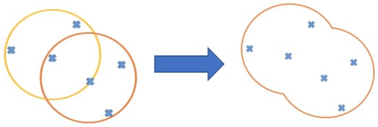
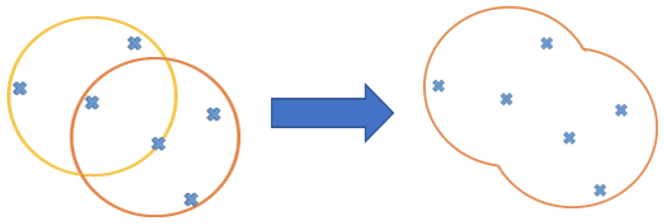
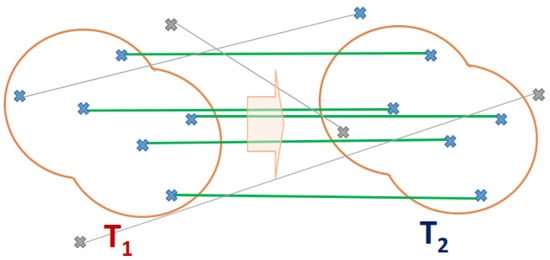
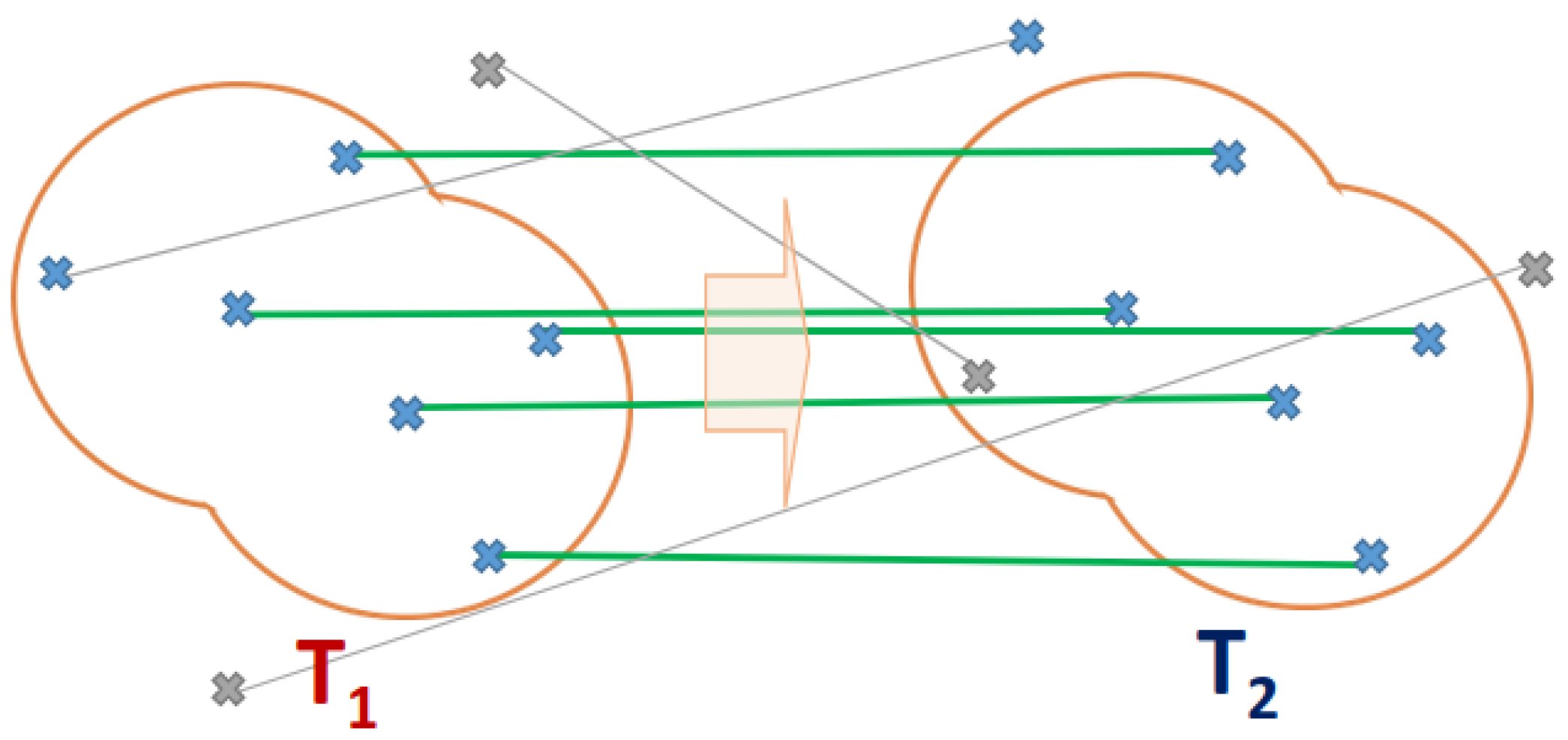
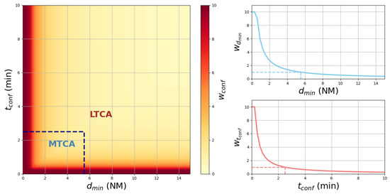
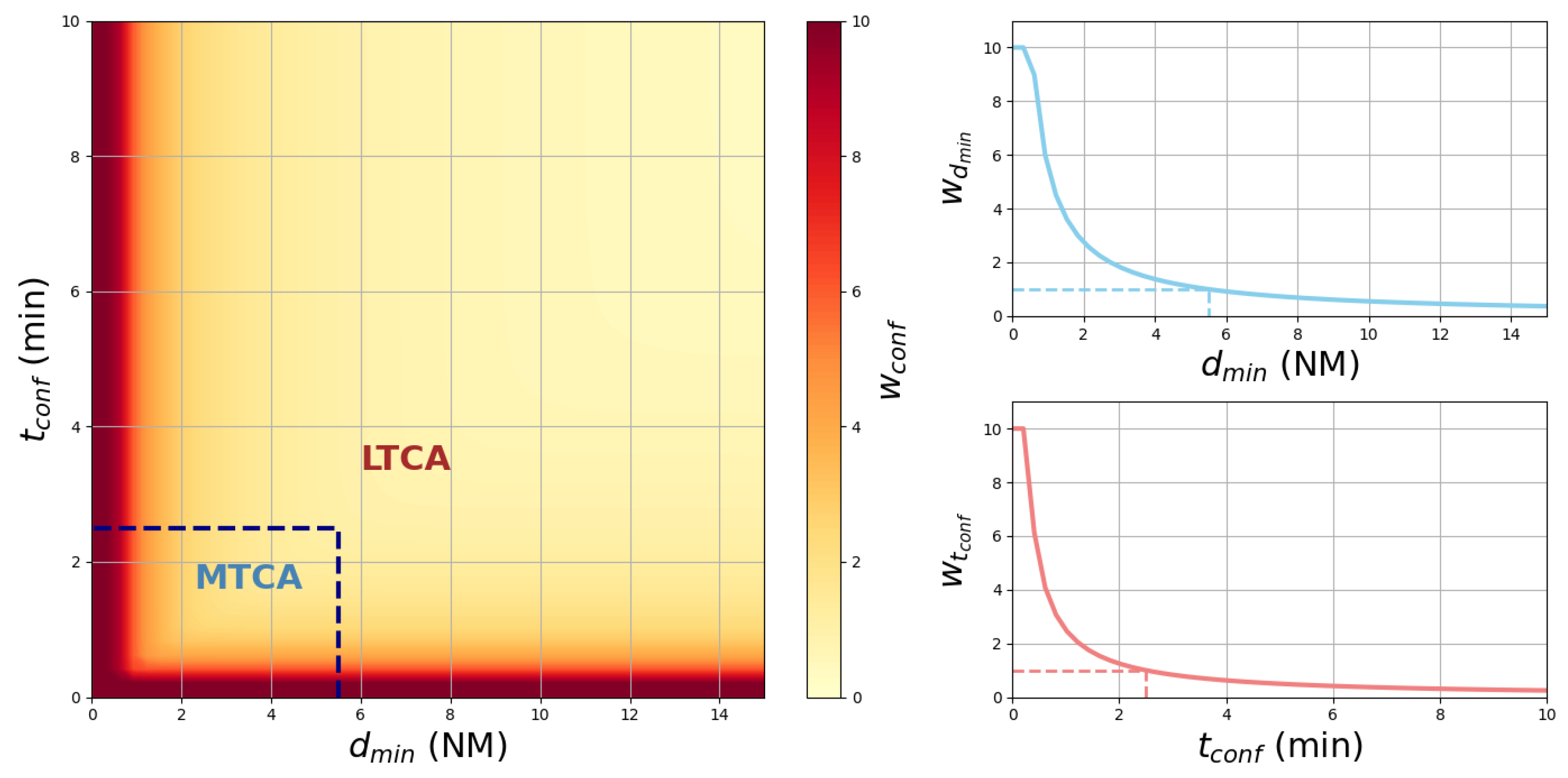
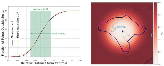
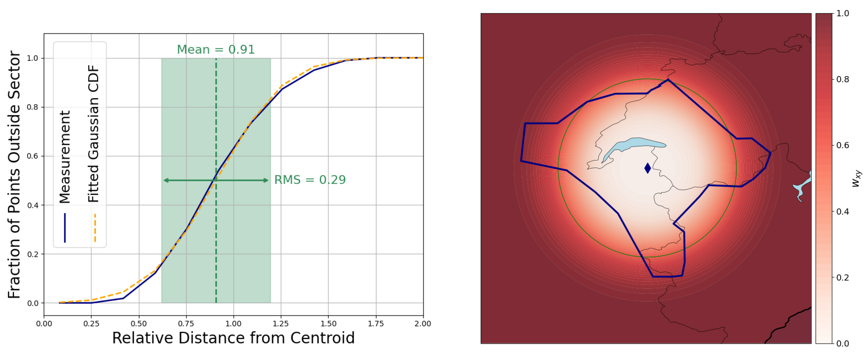
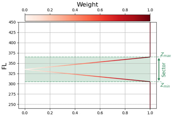
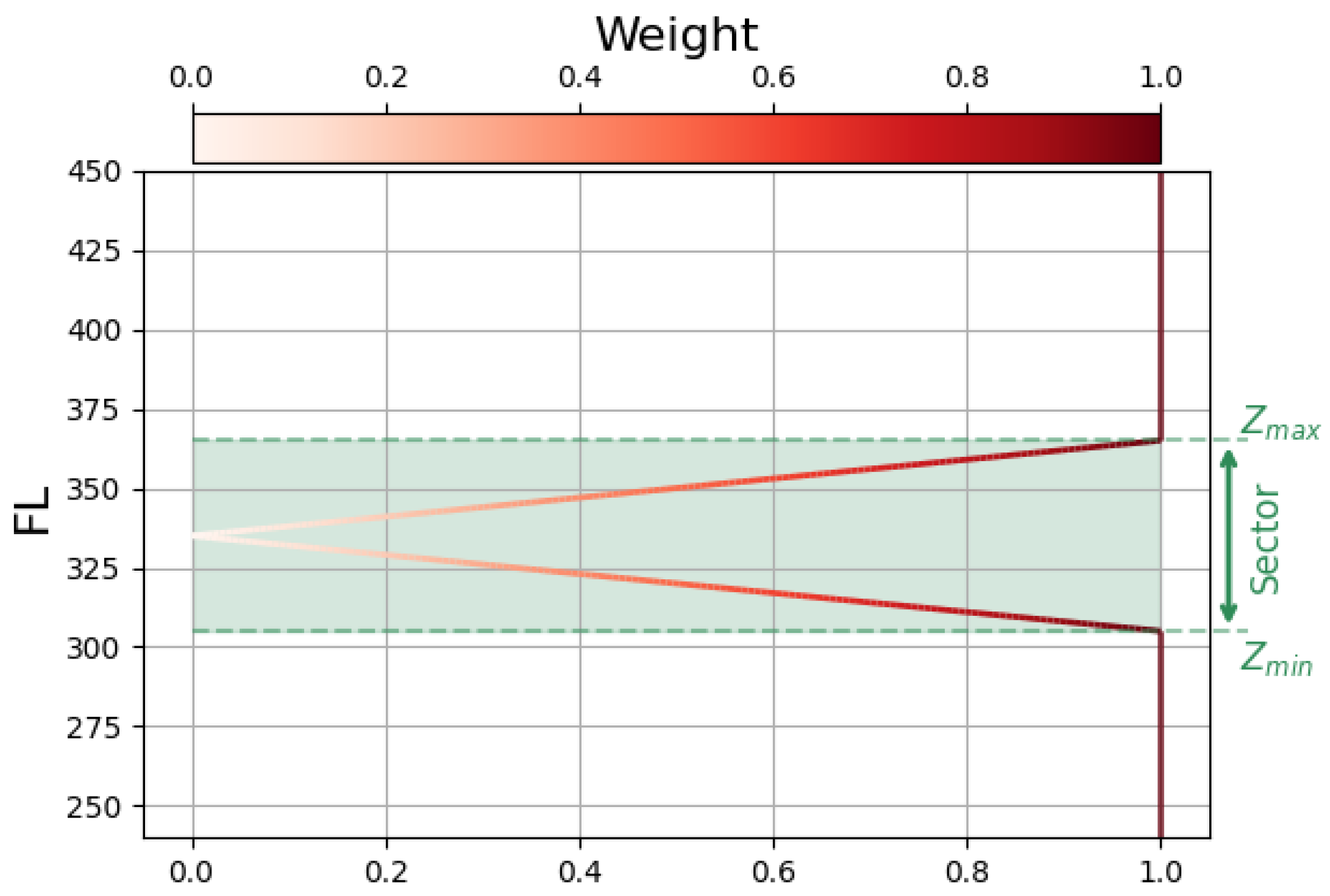
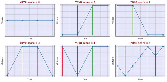
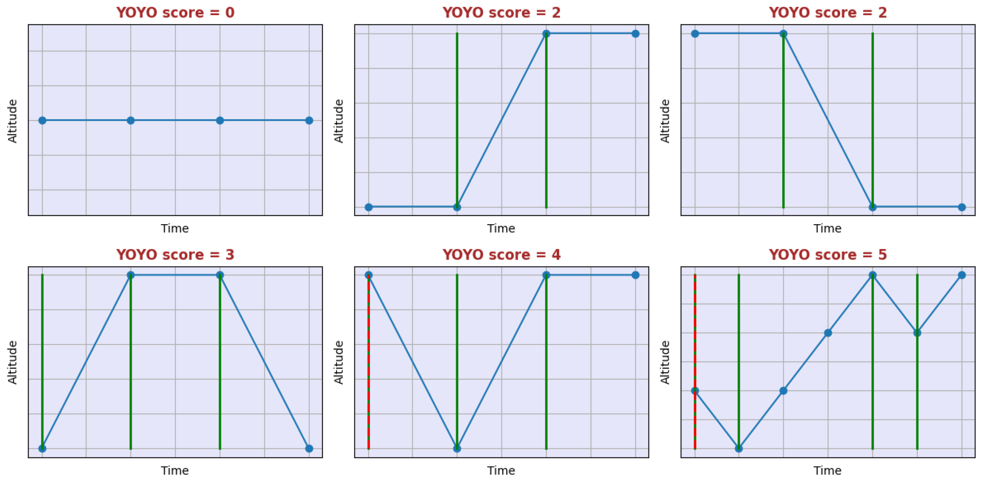
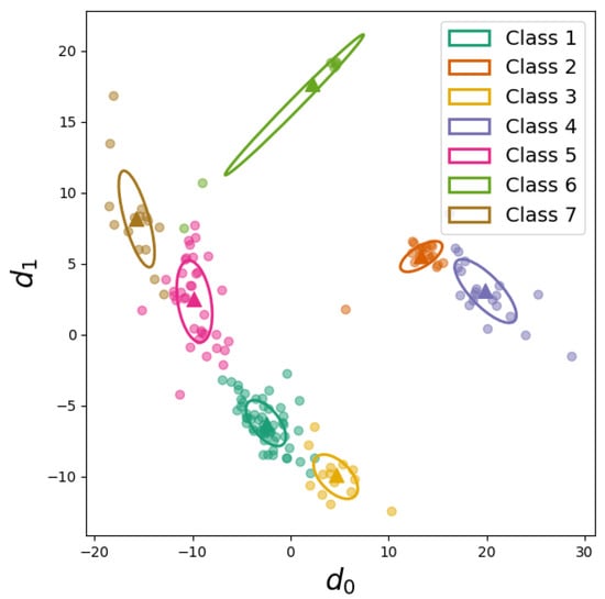
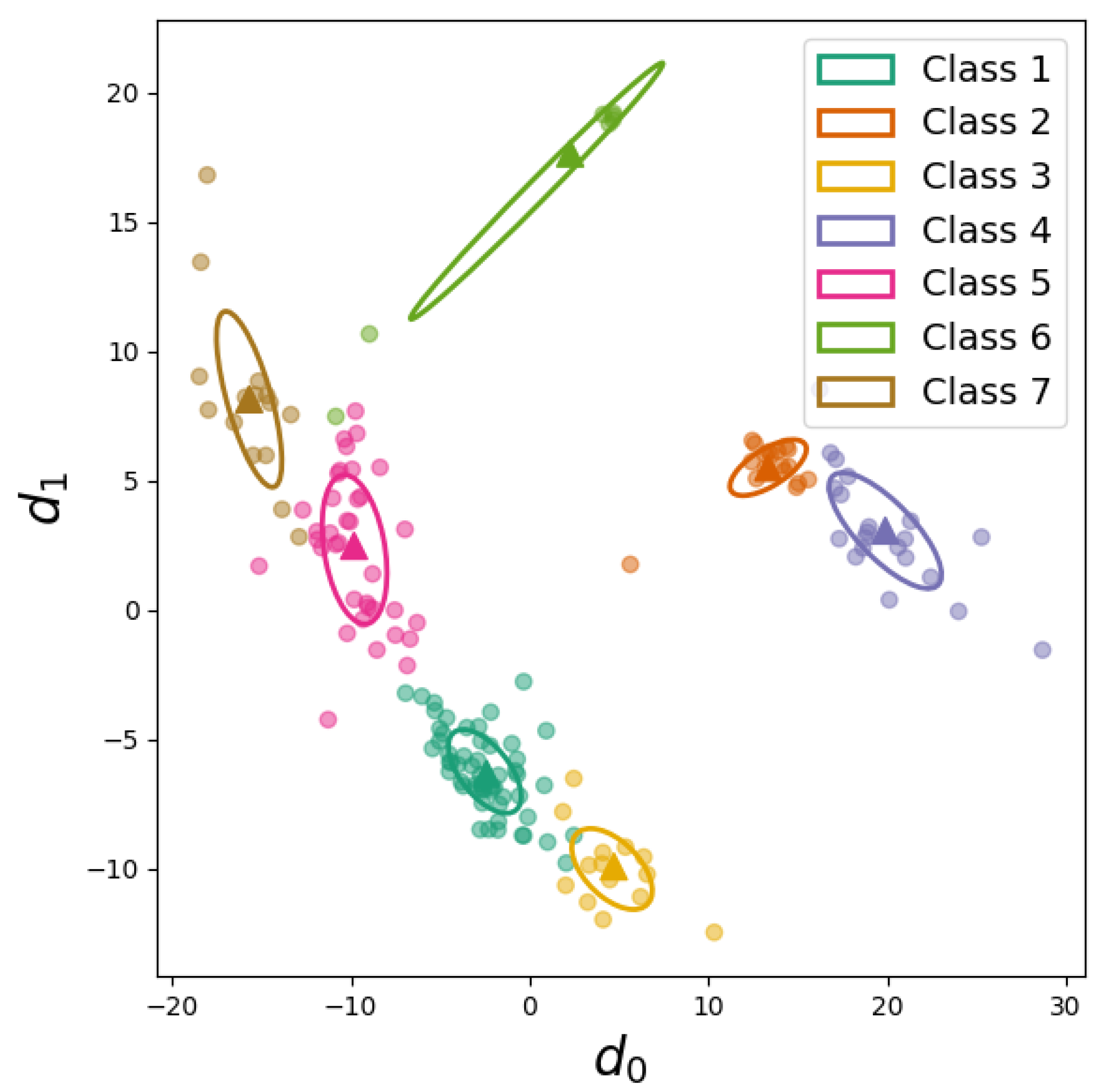
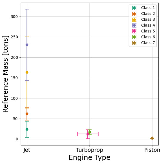
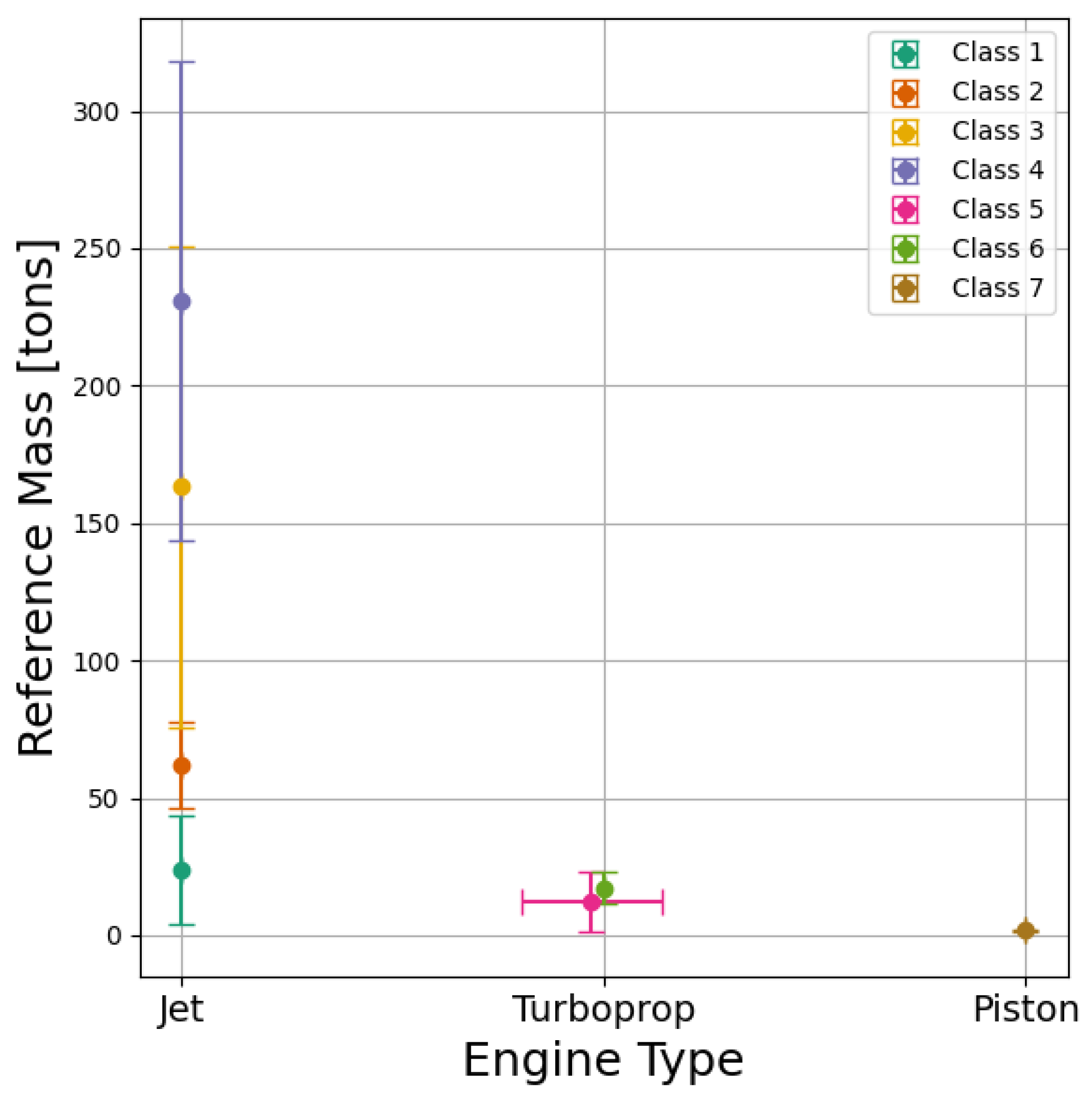
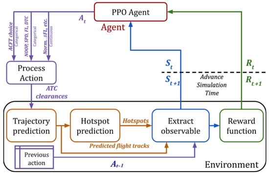
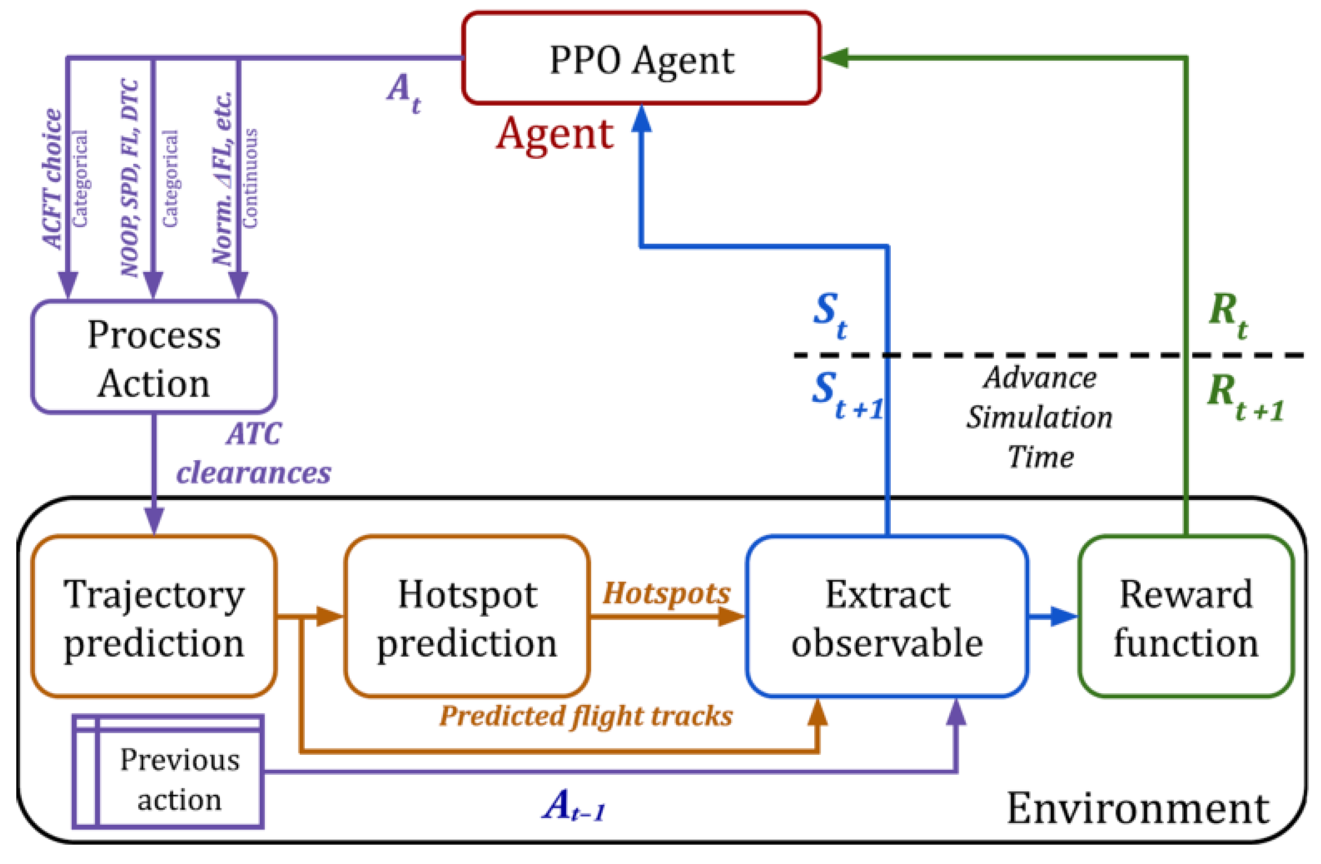
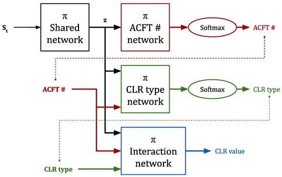
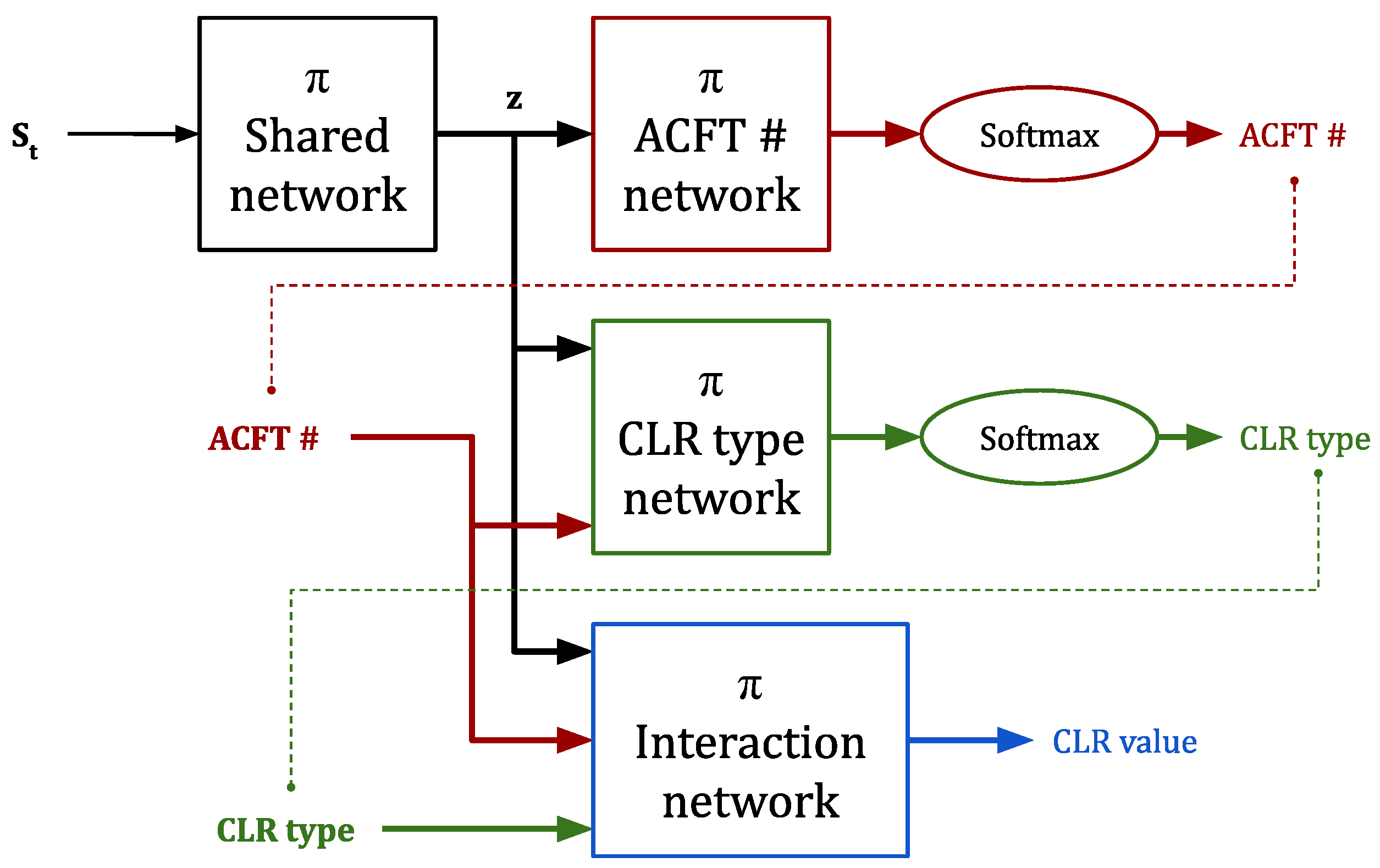
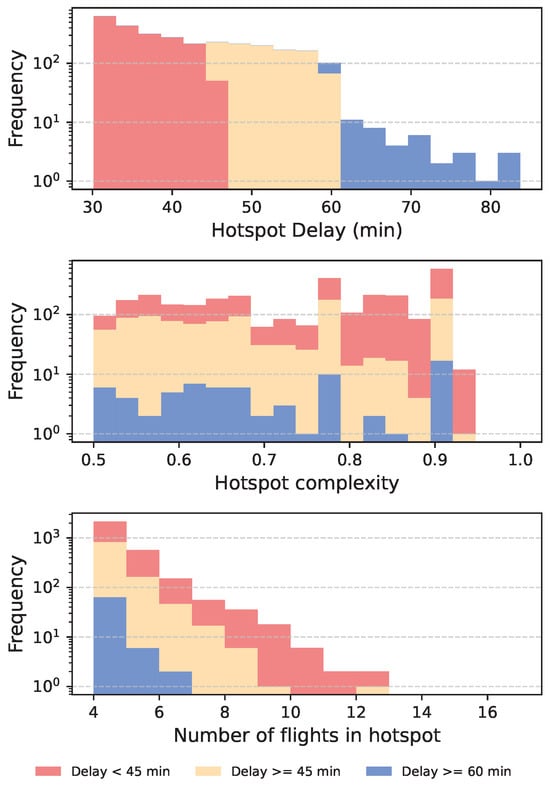
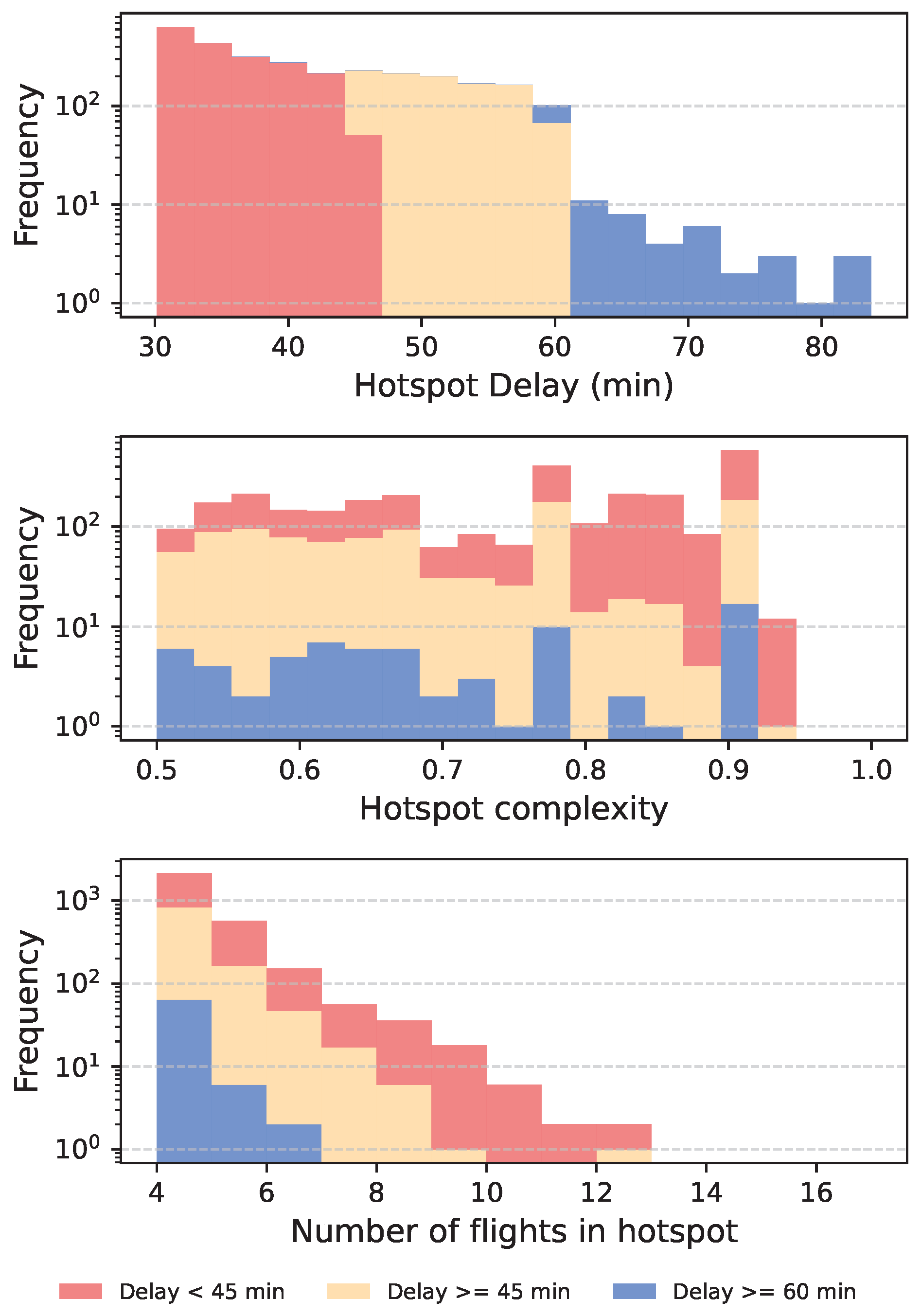
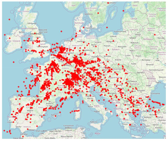
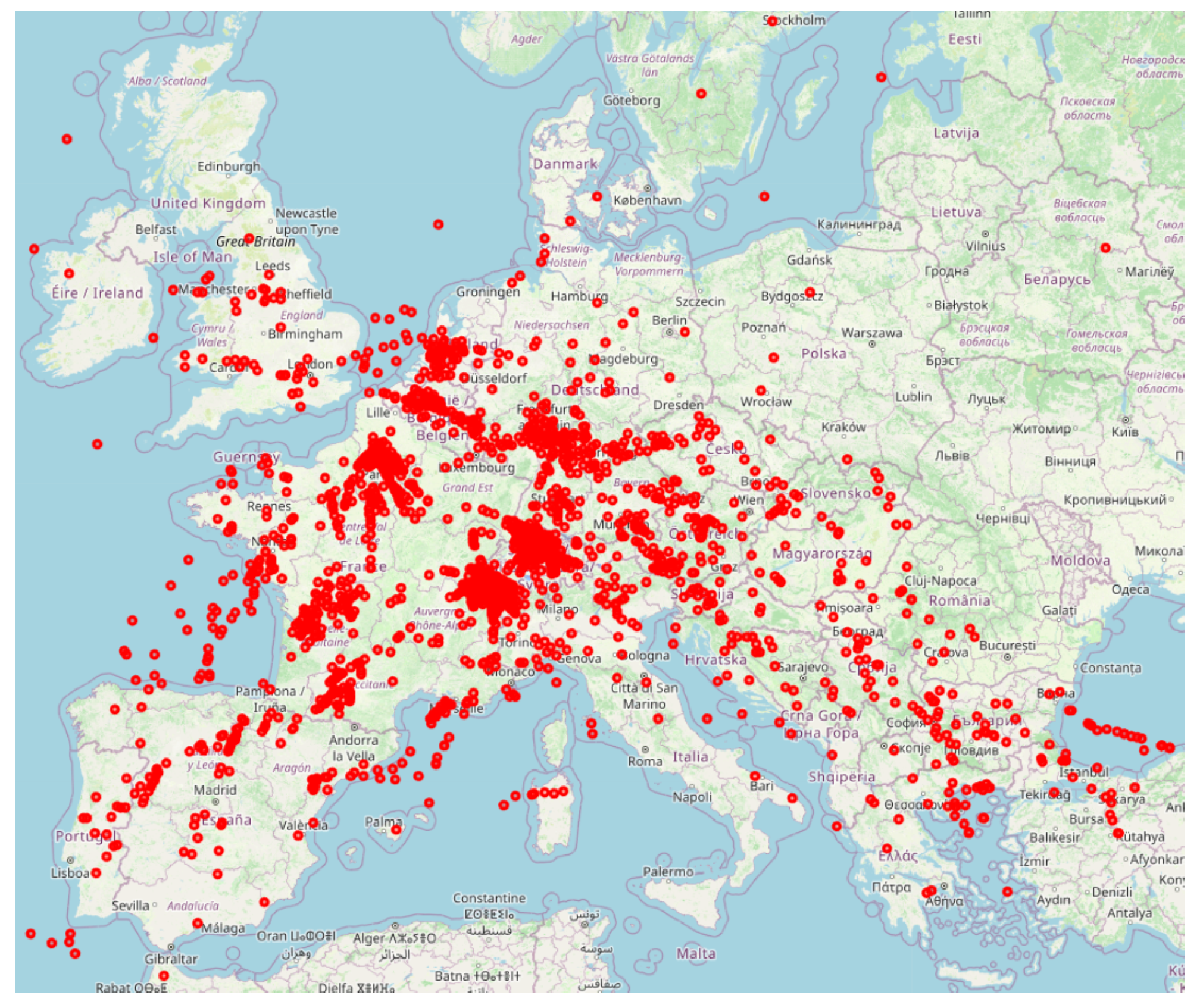
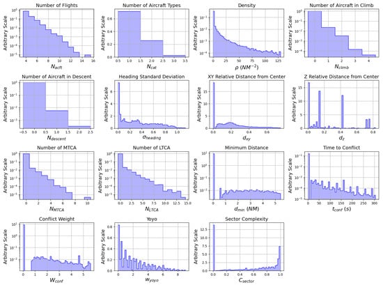
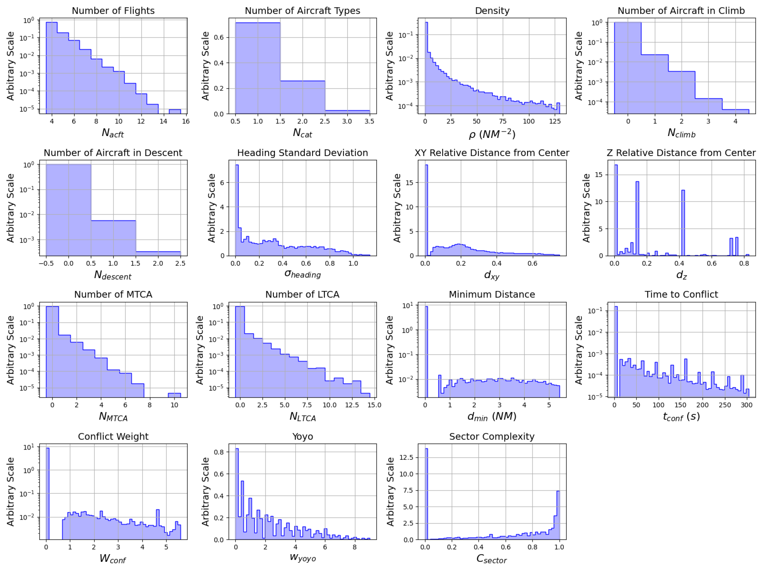
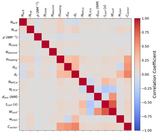
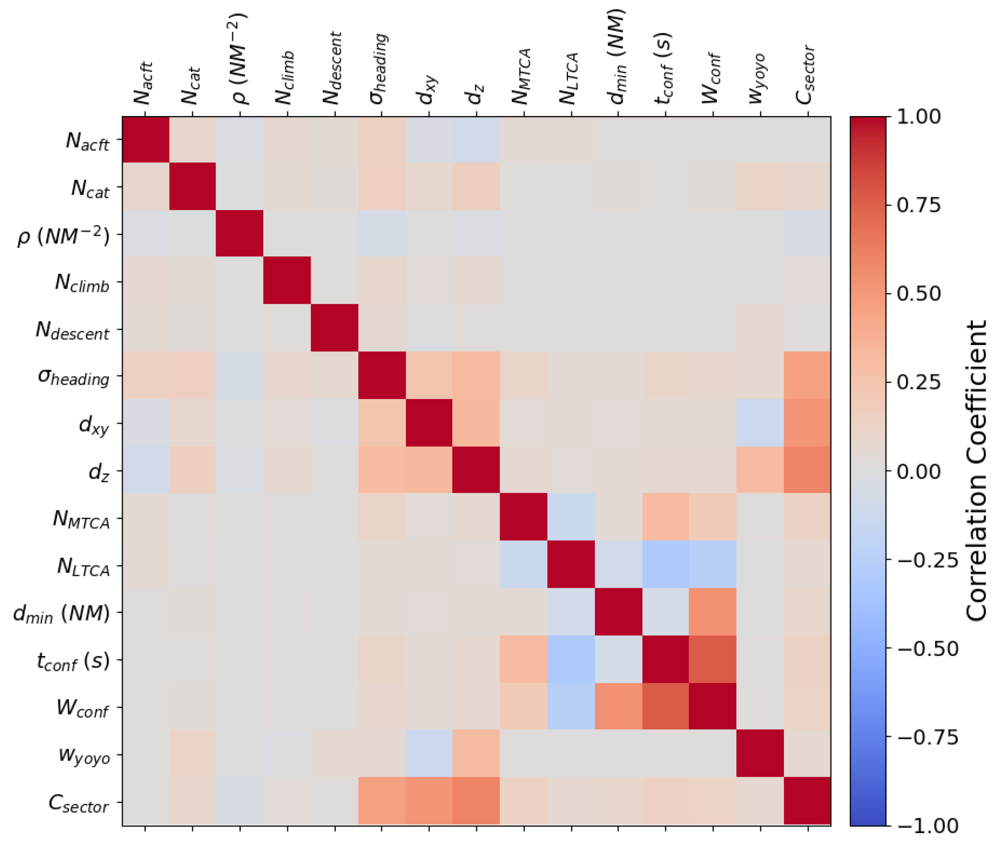
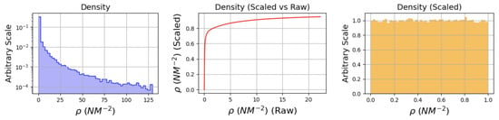
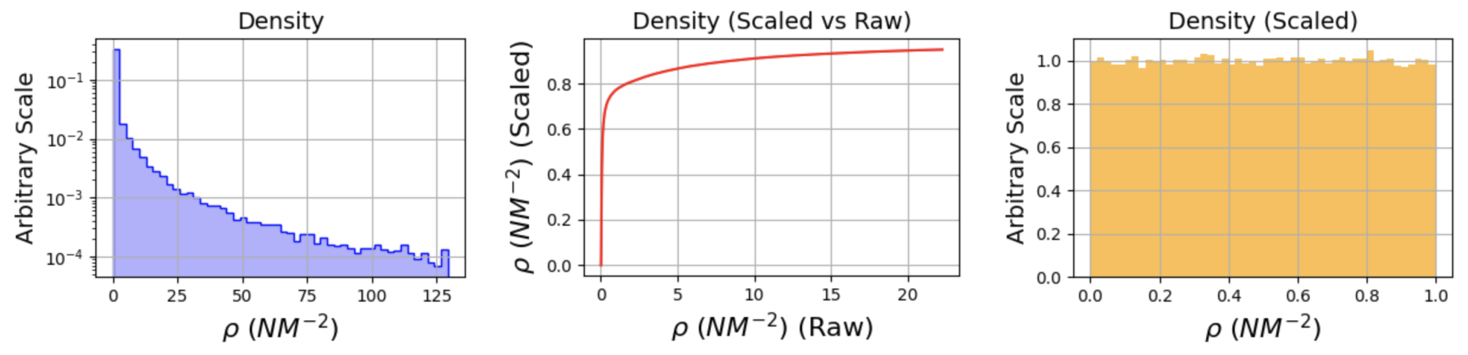
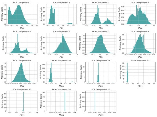
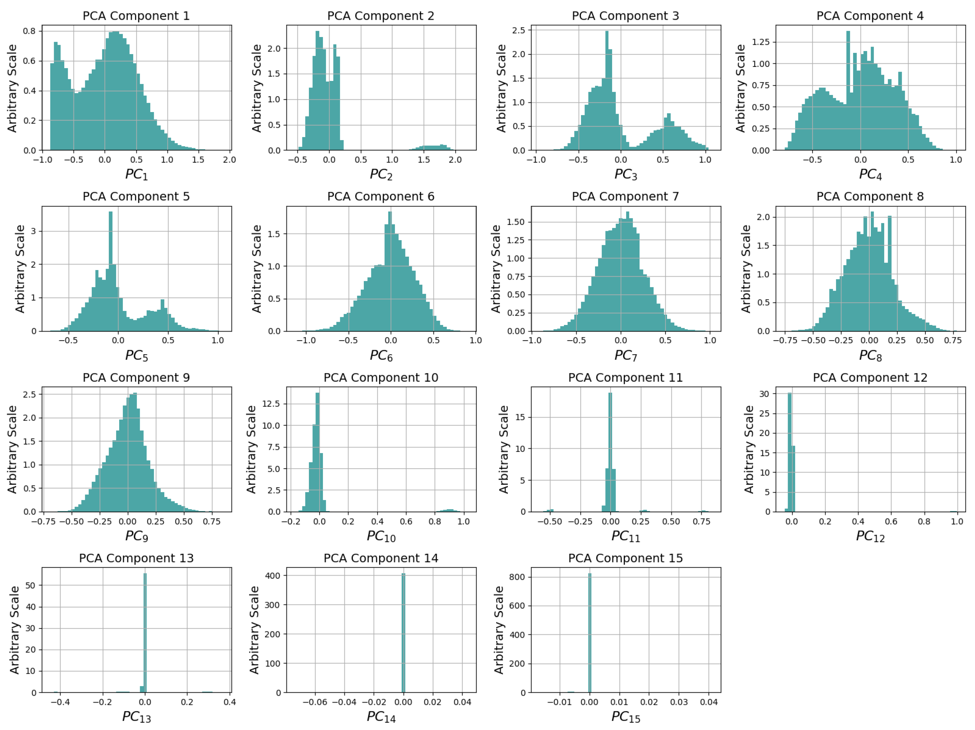
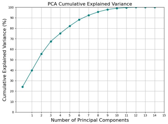
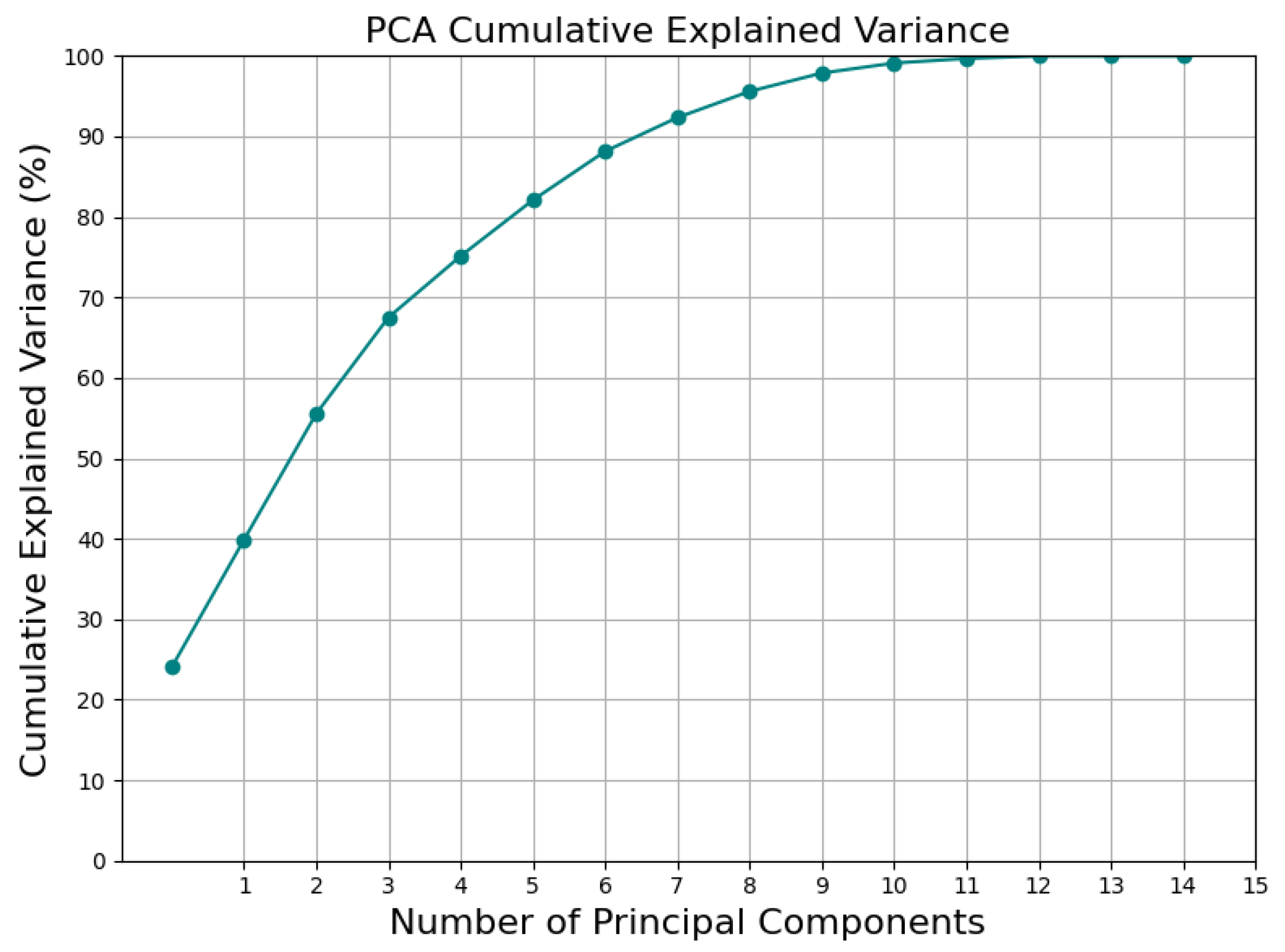
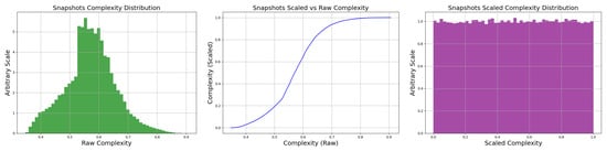
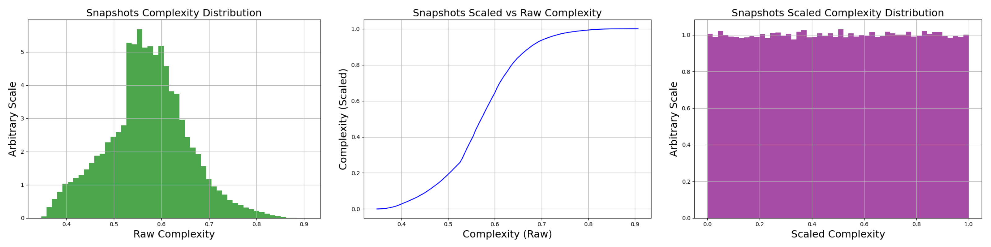
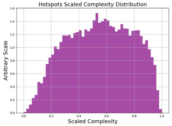
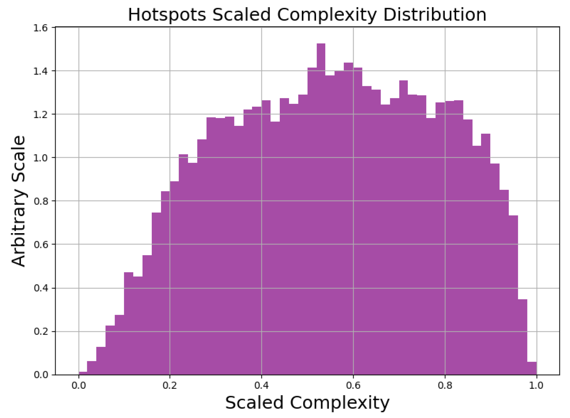
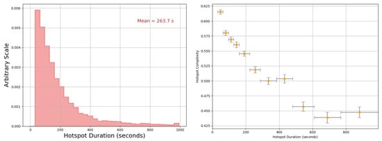
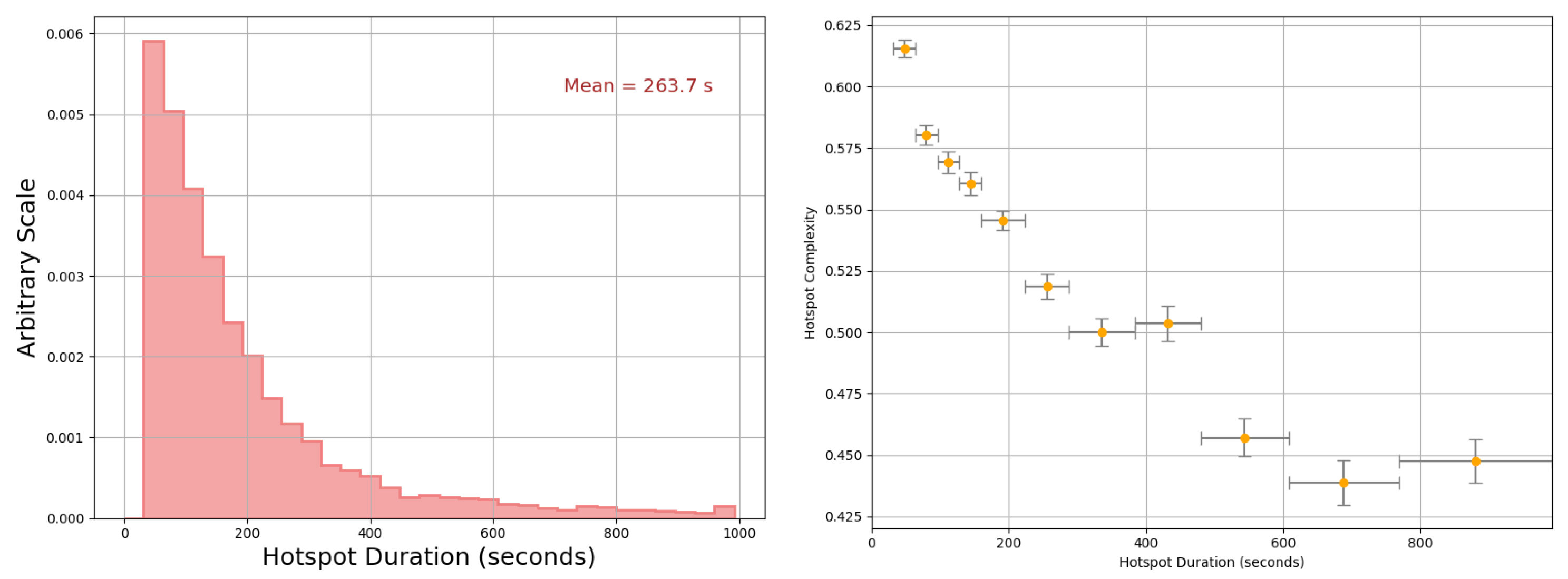
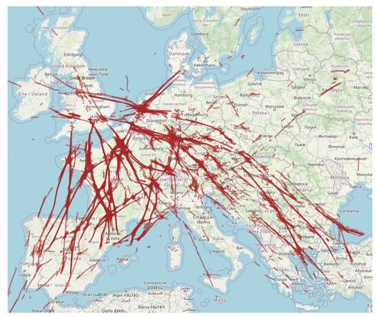
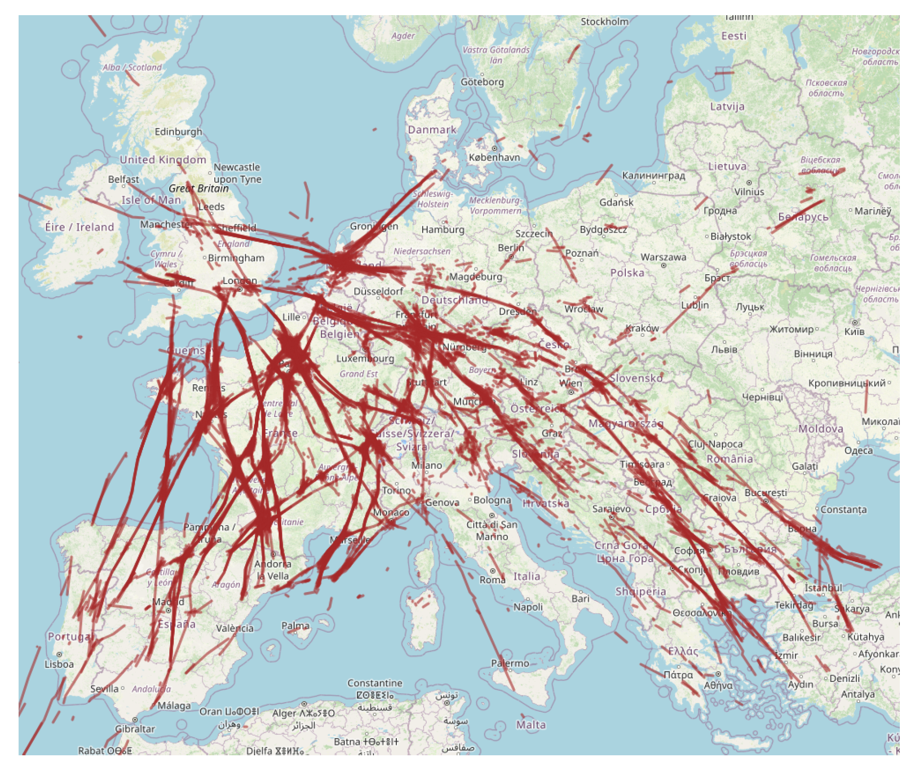
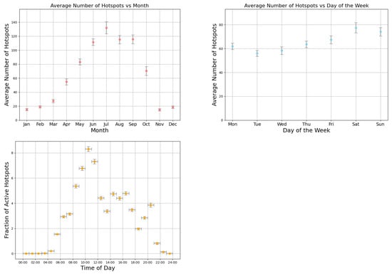
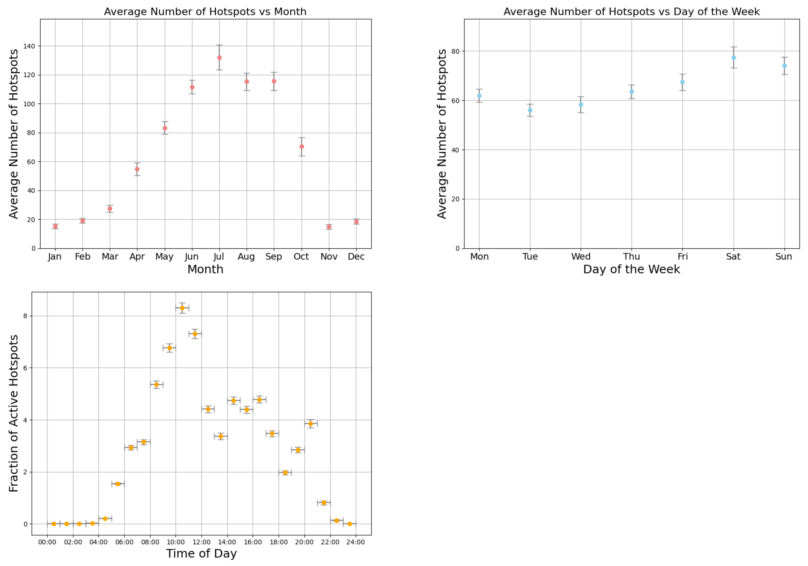
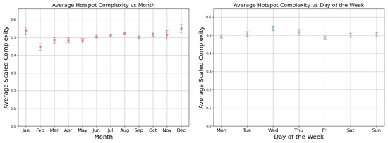
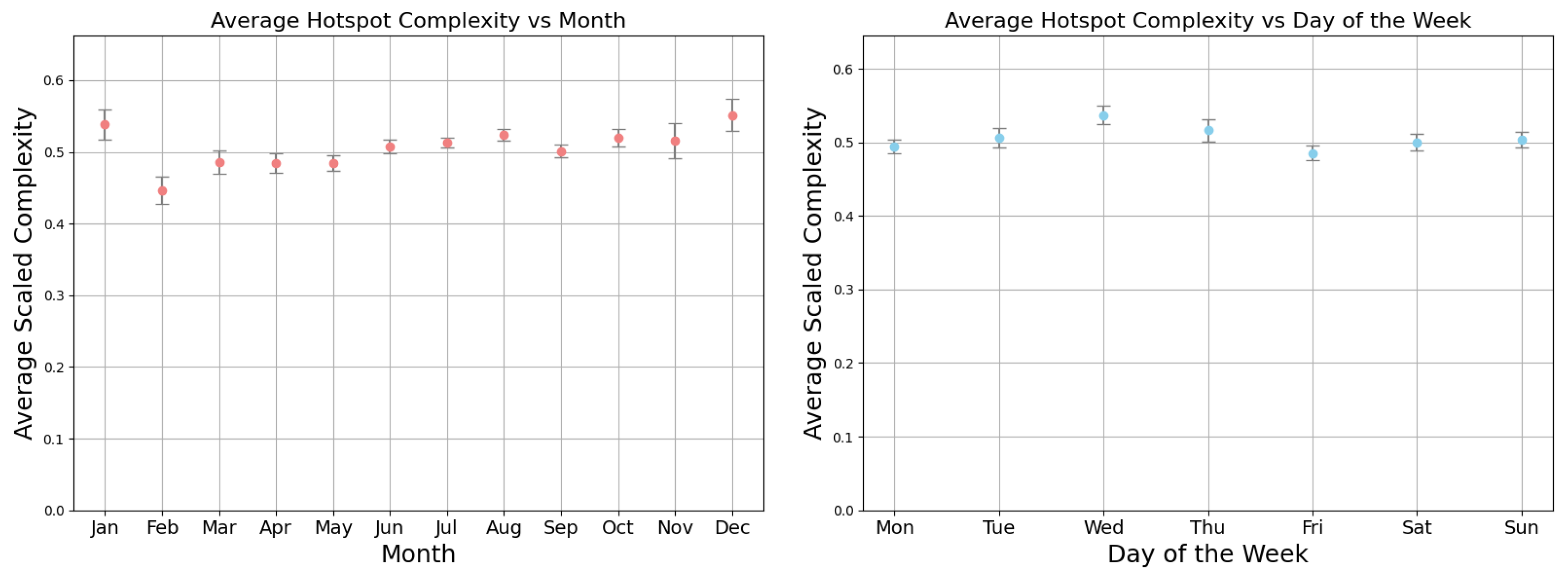
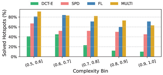
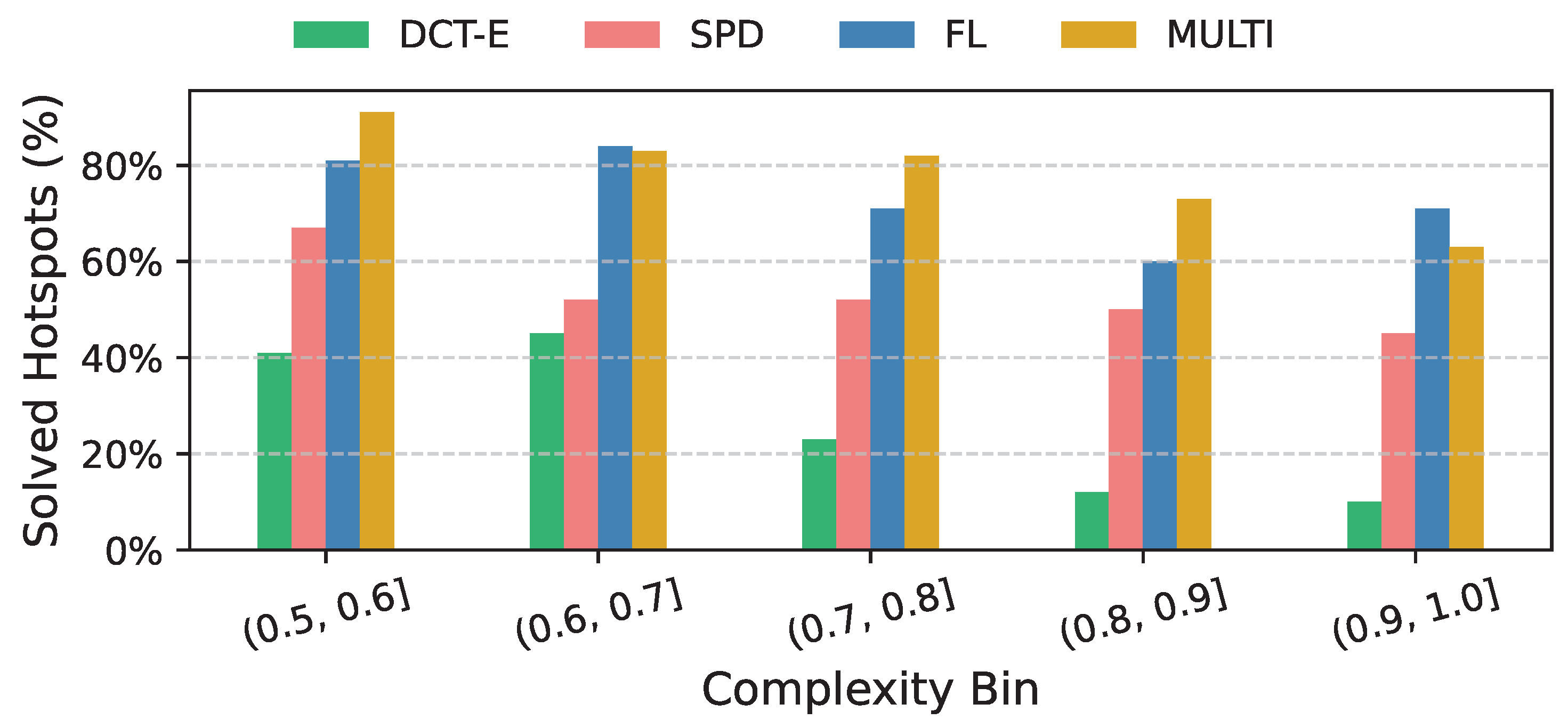
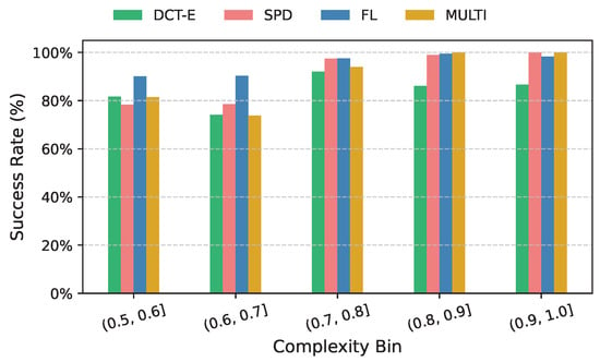
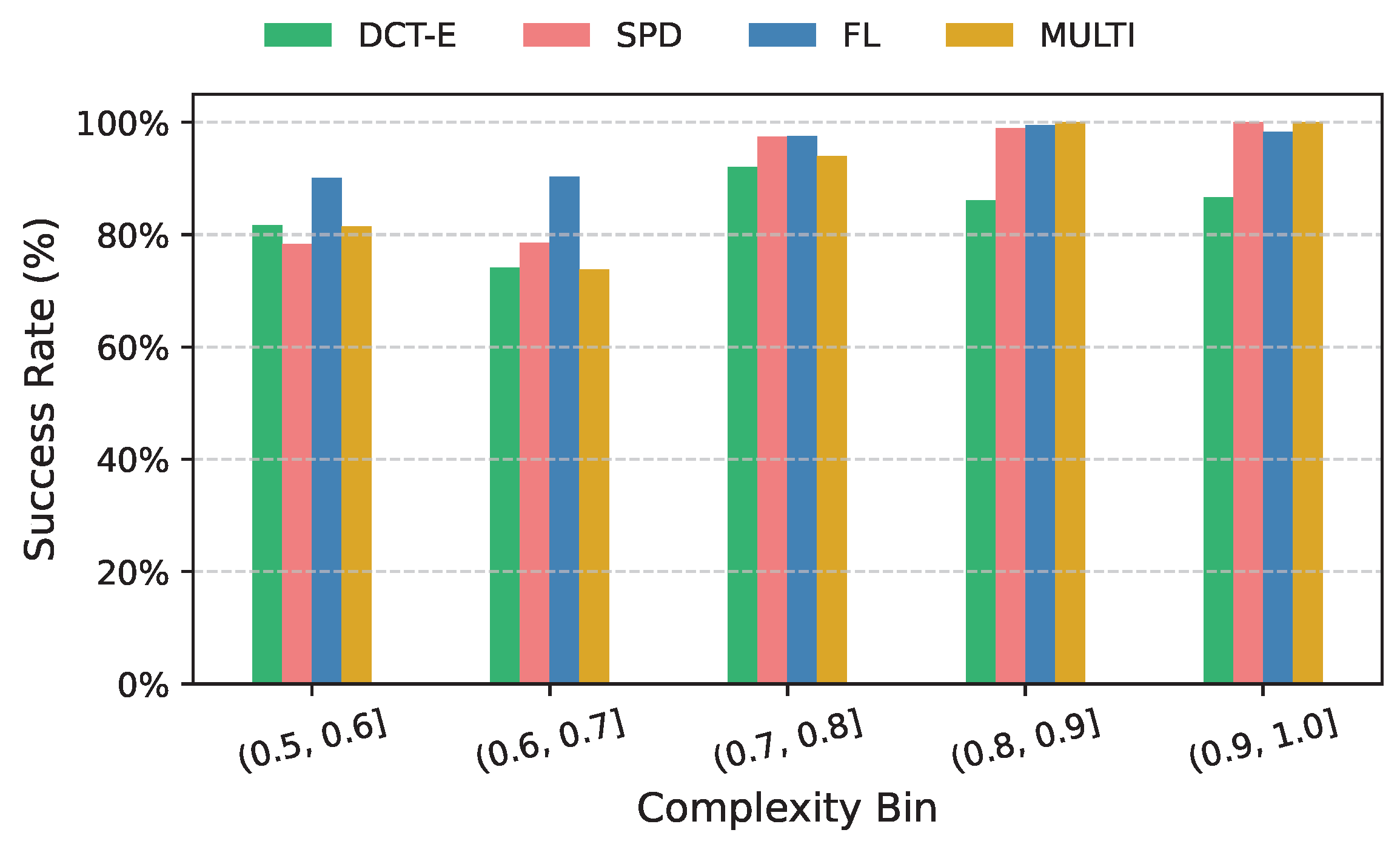
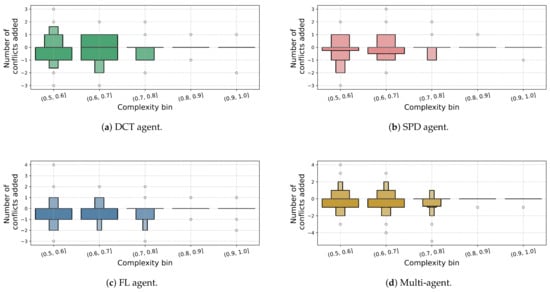
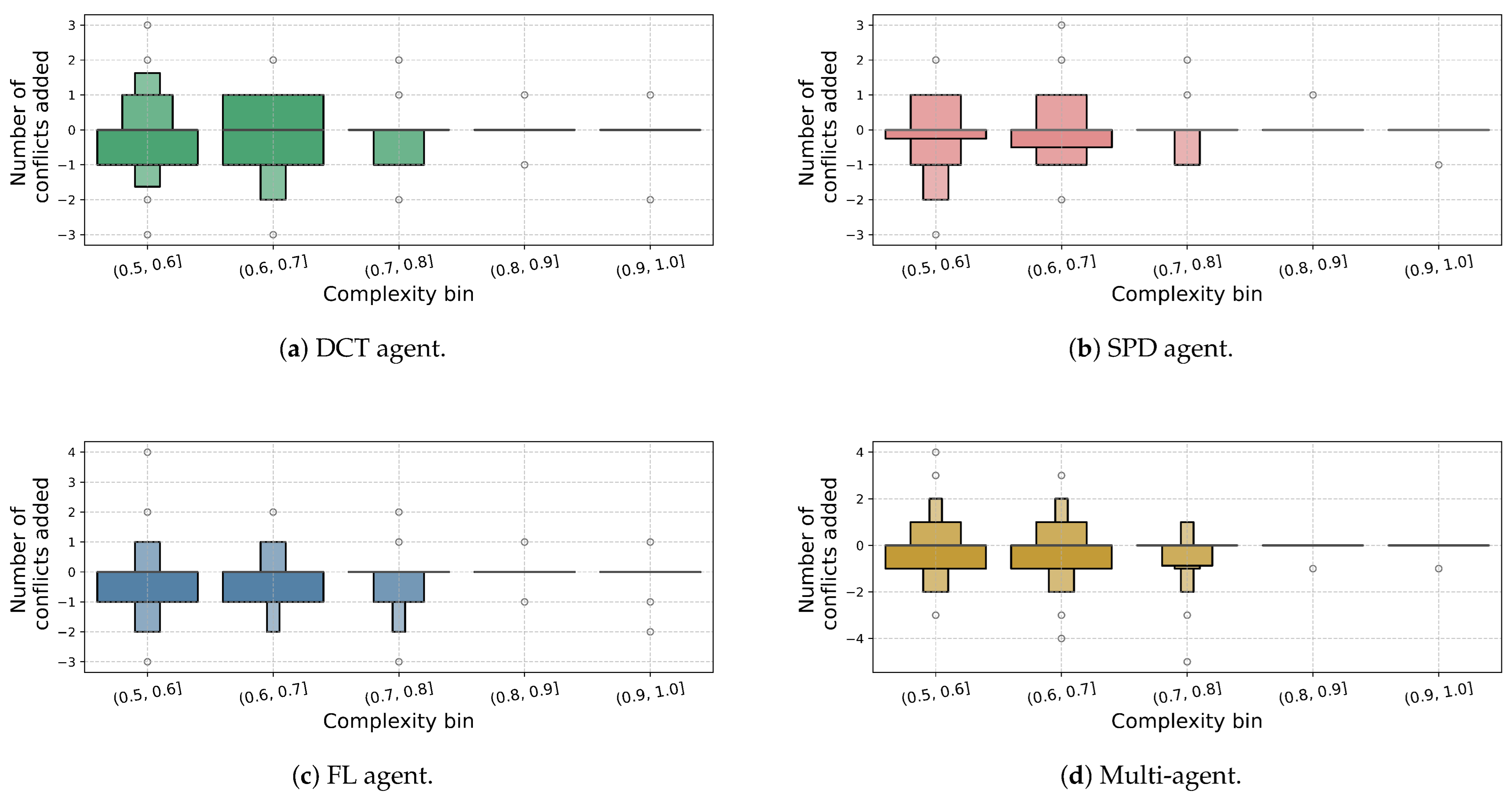
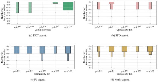
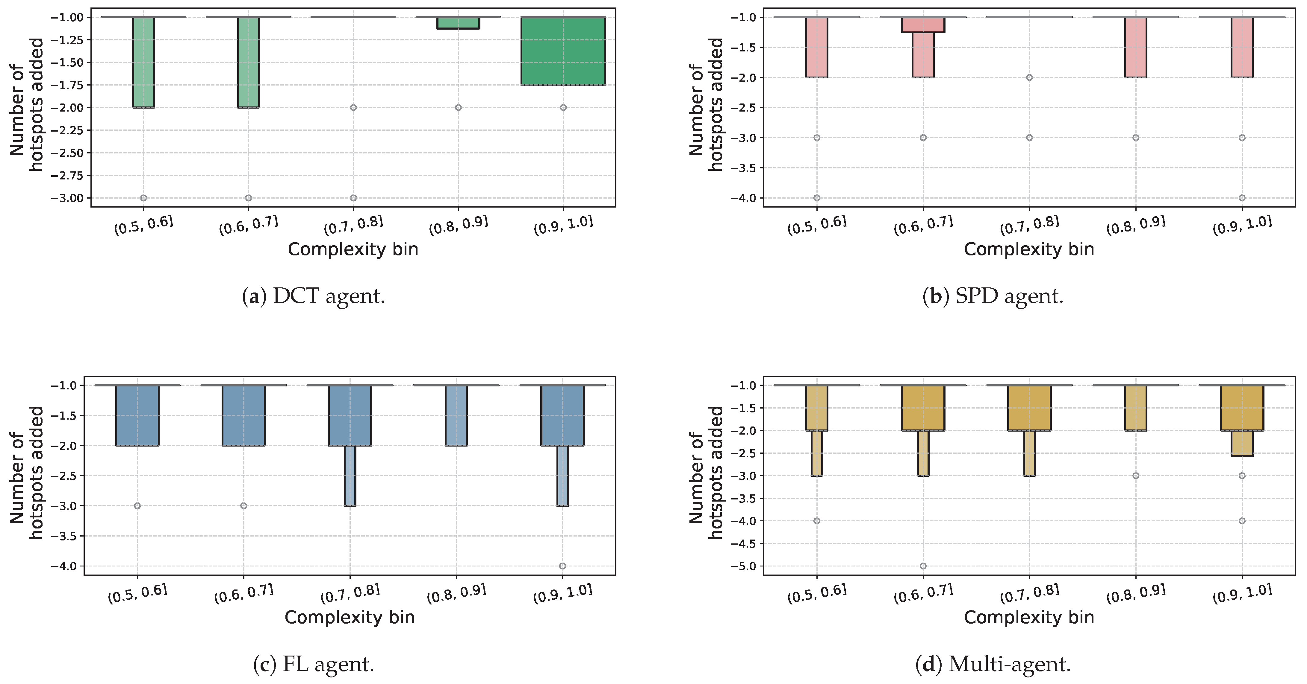
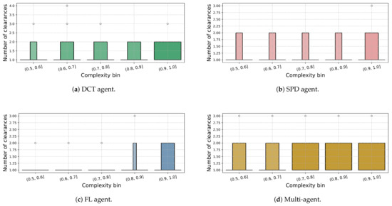
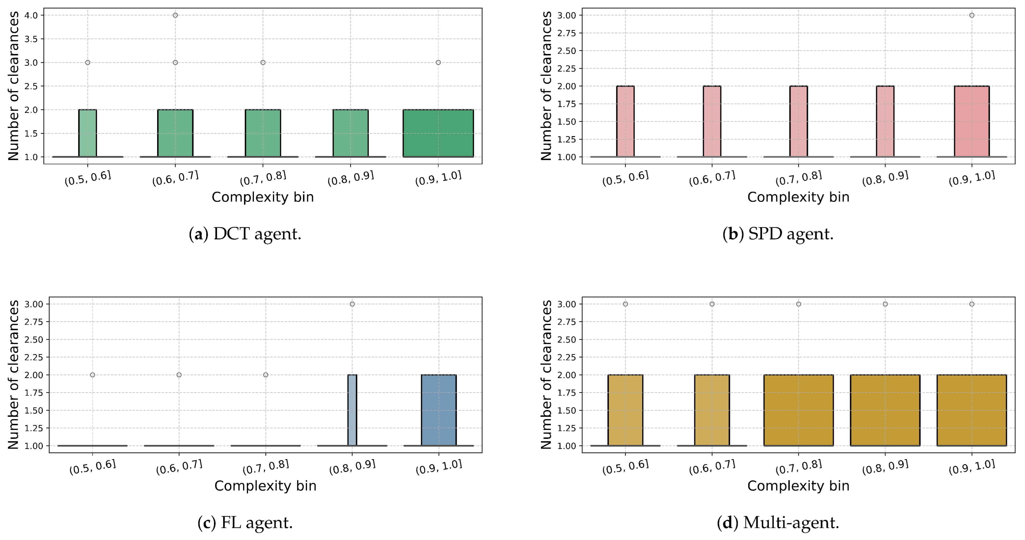
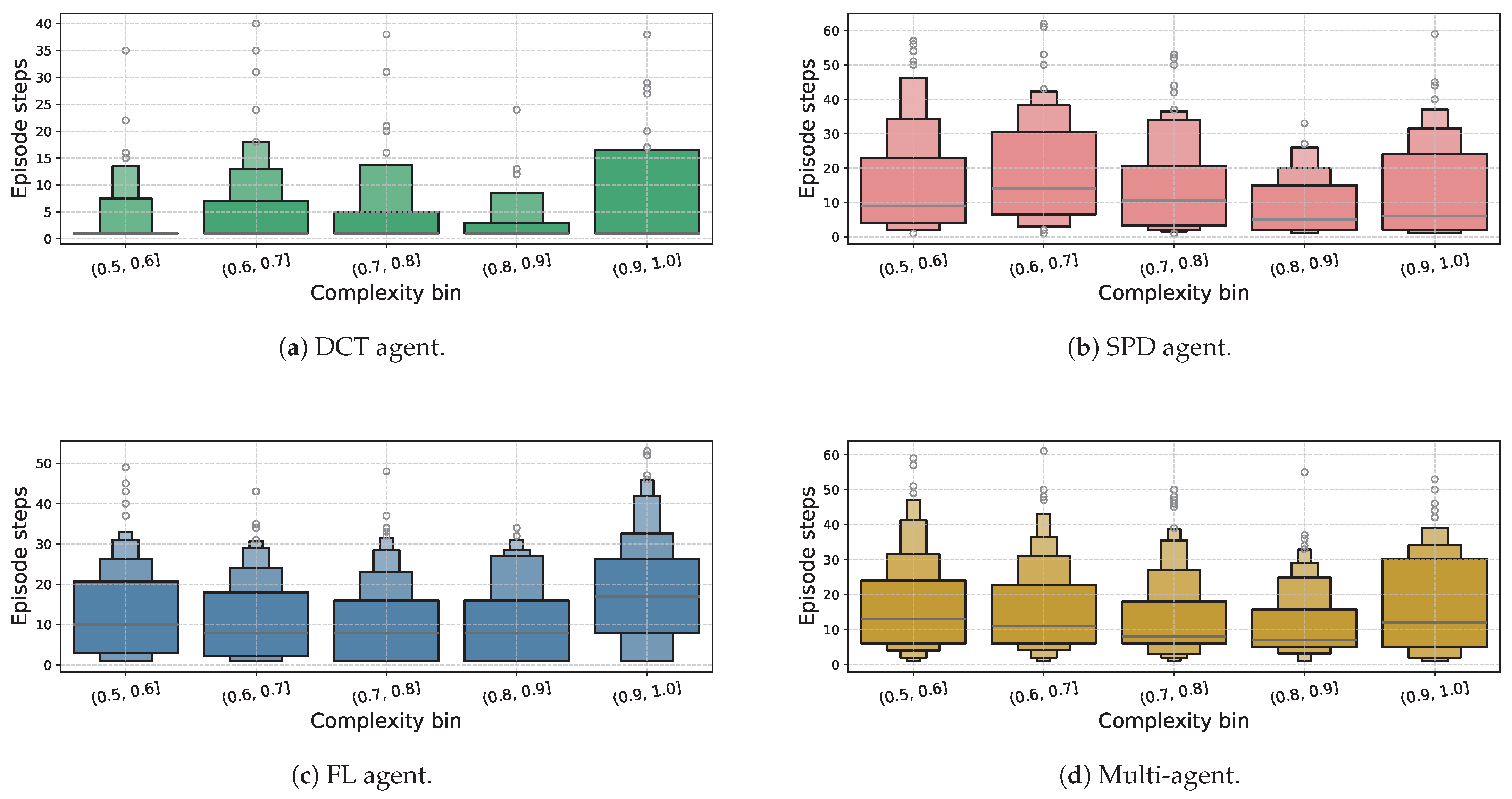
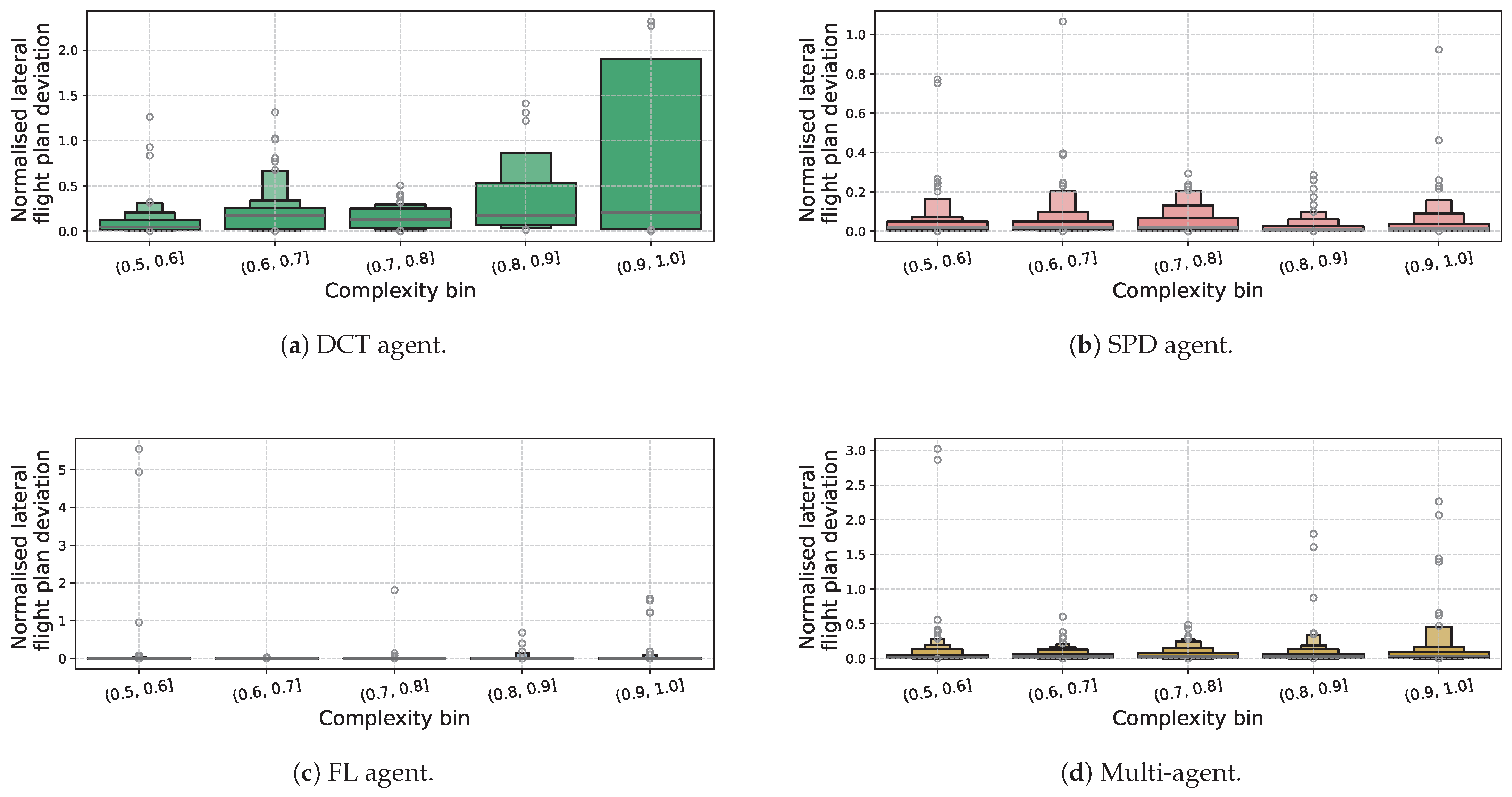
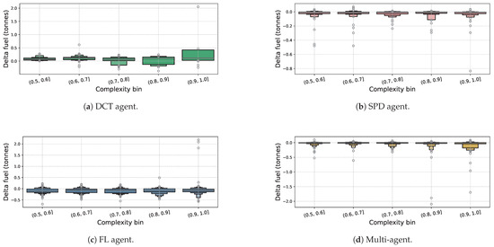
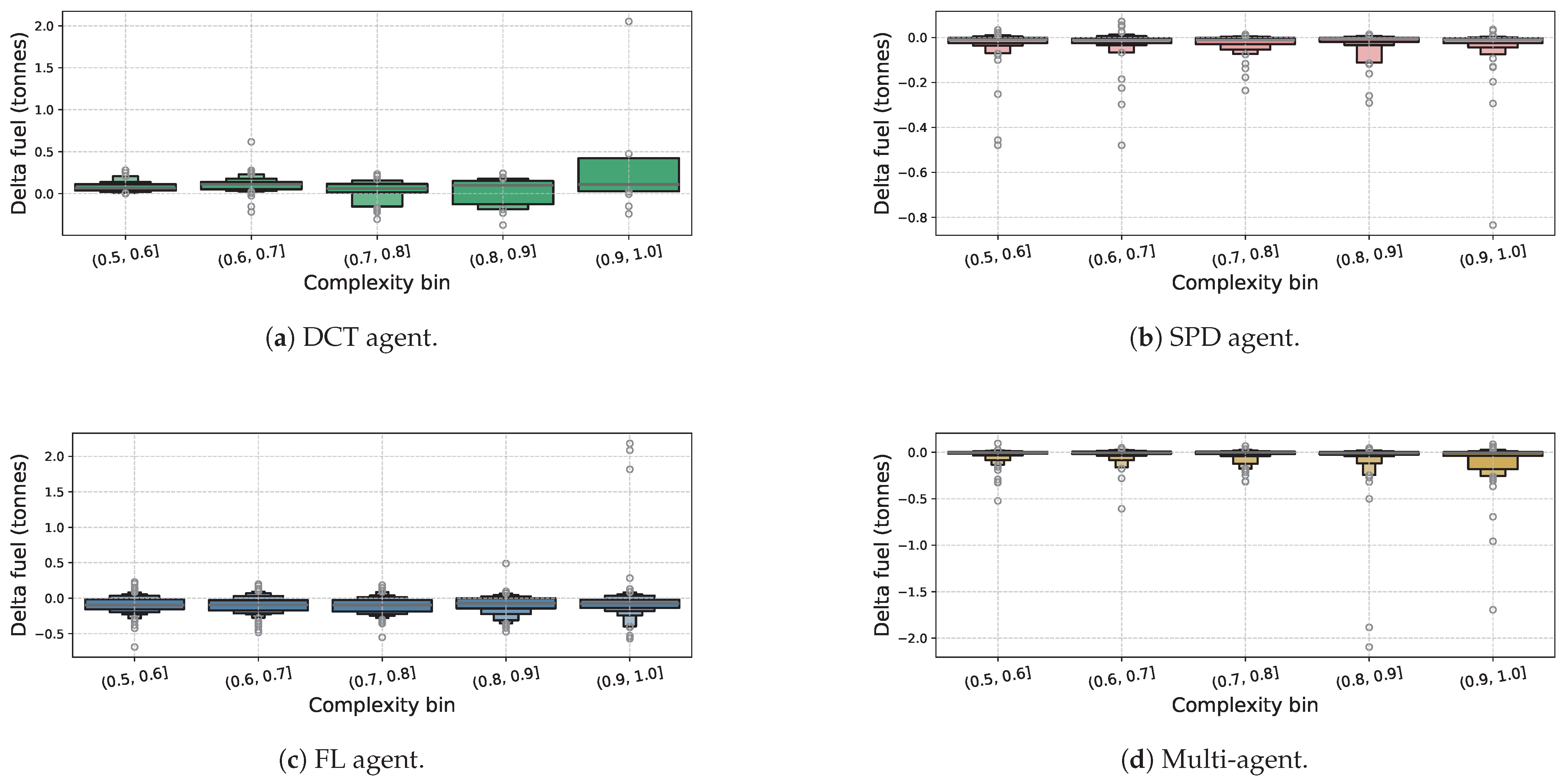
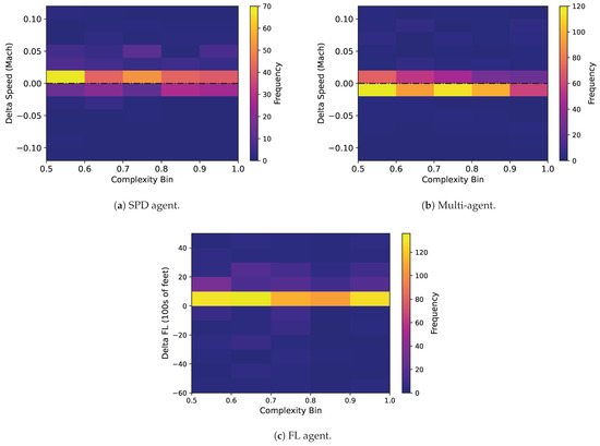
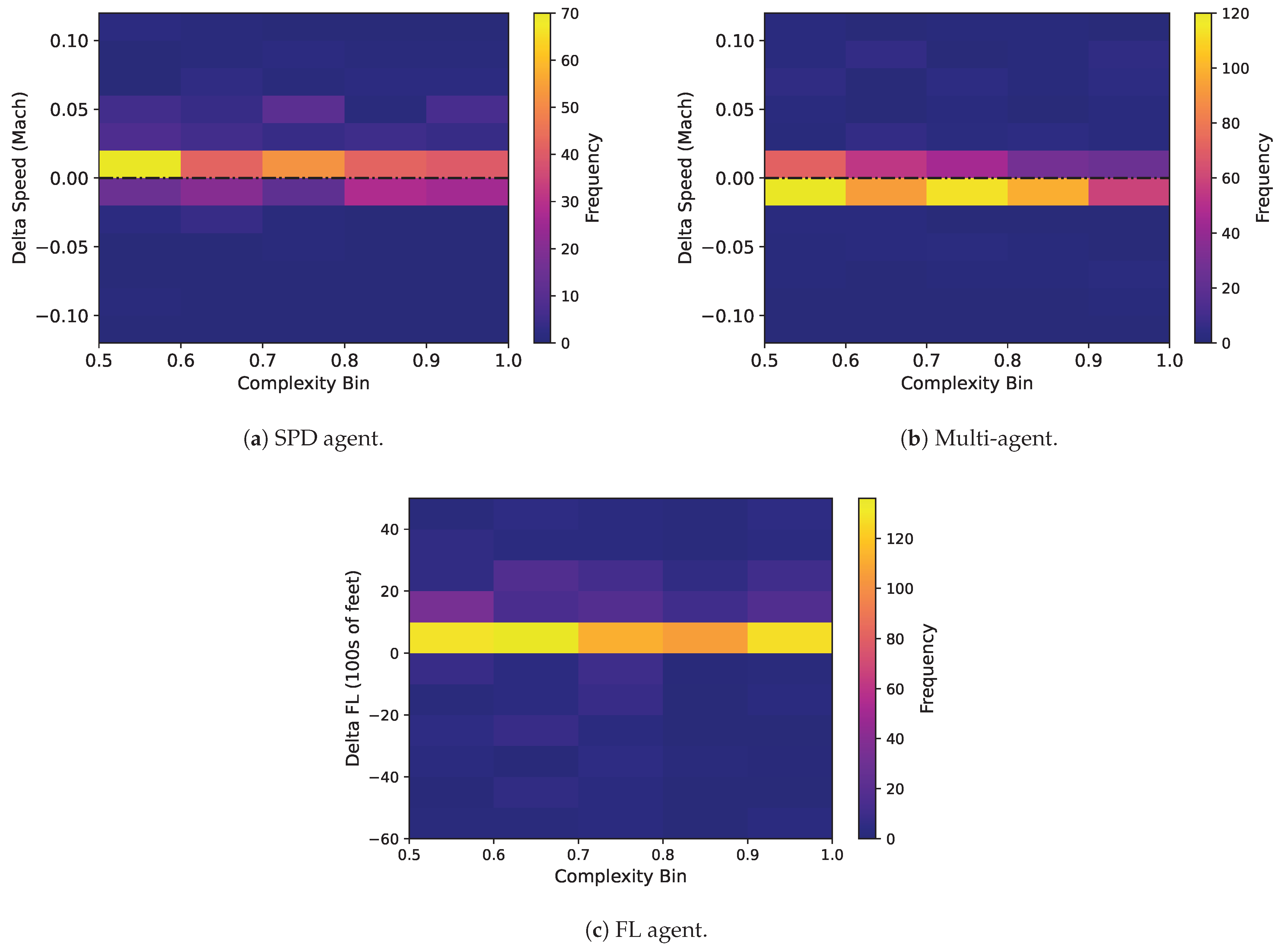
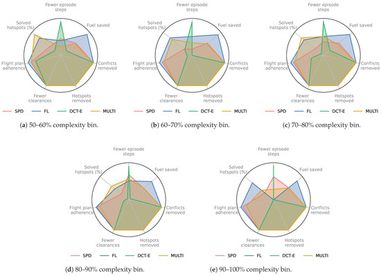
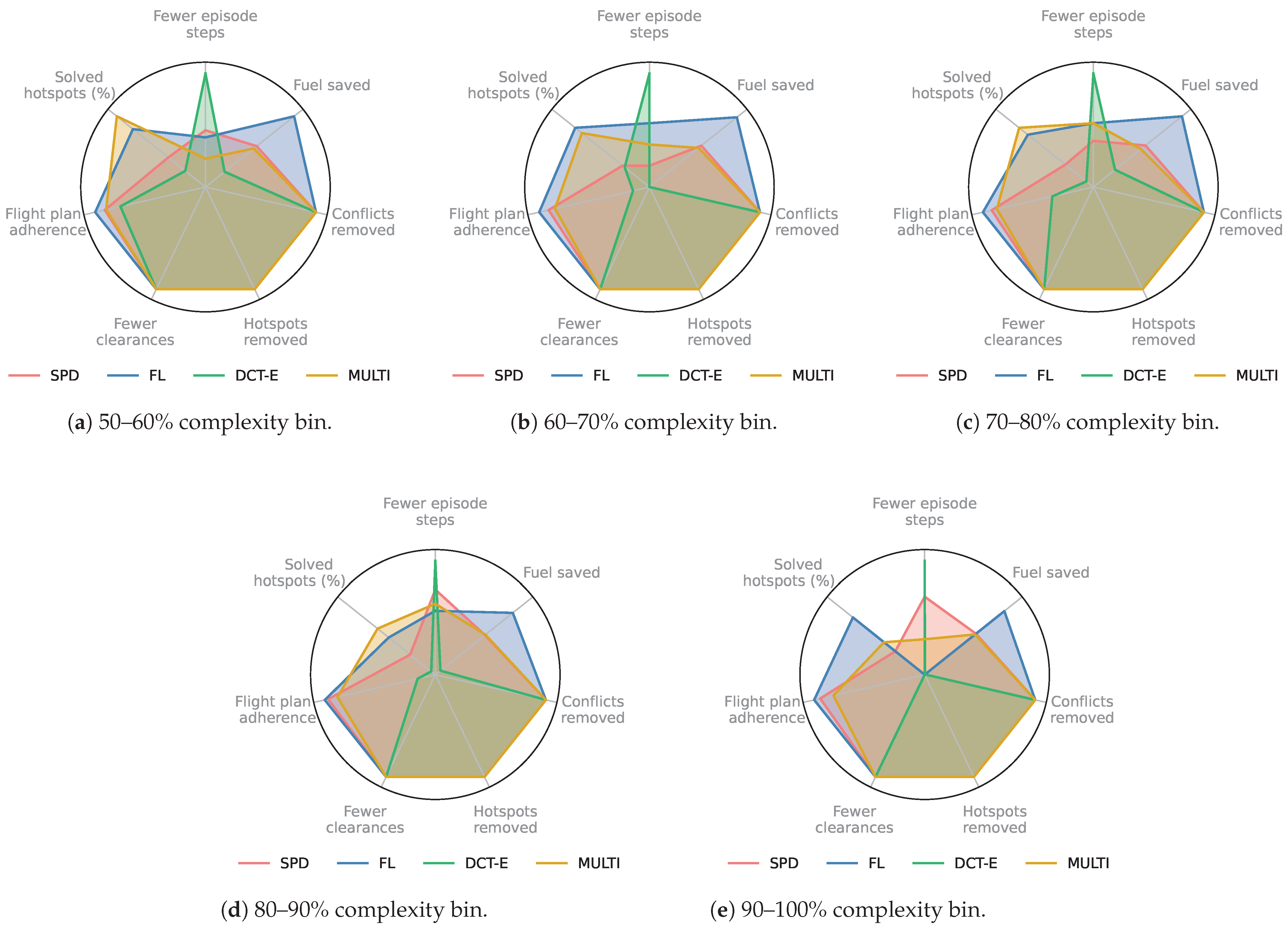

Disclaimer/Publisher’s Note: The statements, opinions and data contained in all publications are solely those of the individual author(s) and contributor(s) and not of MDPI and/or the editor(s). MDPI and/or the editor(s) disclaim responsibility for any injury to people or property resulting from any ideas, methods, instructions or products referred to in the content. |
© 2026 by the authors. Licensee MDPI, Basel, Switzerland. This article is an open access article distributed under the terms and conditions of the Creative Commons Attribution (CC BY) license.