


Abstract
Agricultural drought represents a critical threat to water-dependent economies in arid Andean regions; however, forecasting tools tailored to data-scarce, high-altitude basins remain limited. This study developed and evaluated a multi-model spatiotemporal framework for agricultural drought forecasting in Candarave, in the northern Atacama Desert; we forecast the 3-month Standardized Precipitation–Evapotranspiration Index (SPEI-3) one month ahead (lead time t + 1) for an agricultural, data-scarce Andean basin. Seven modeling approaches were compared: three machine learning baselines (XGBoost, Random Forest, and Elastic Net), two statistical time-series models (ARIMA and ARIMAX), and two deep learning architectures (CNN-LSTM and ConvRNN). A driver analysis based on Elastic-Net coefficients identified spatiotemporal persistence (SPEI_neighbor, SPEI_lag1), precipitation, maximum temperature, and the Coastal El Niño Index (ICEN) as the dominant drought predictors. ARIMAX achieved the best overall performance (RMSE = 0.377; R2 = 0.909; NSE = 0.909; KGE = 0.889), demonstrating that incorporating exogenous climatic drivers substantially enhances forecasting skill. Among machine learning baselines, Elastic Net outperformed tree-based models (KGE = 0.924). Deep learning models revealed the weakest performance, with very low R2 values, attributed to insufficient training data, overparameterization, and the predominantly linear and persistence-driven nature of drought dynamics in Candarave. Under an operationally realistic configuration (all predictors lagged to forecast time), the approach provides a useful decision-support tool for one-month-ahead agricultural drought early warning, rather than a turnkey operational system.
Keywords:
agricultural drought; forecasting; driver analysis; Random Forest; XGBoost; Elastic Net; ARIMA; ARIMAX; CNN-LSTM; ConvRNN 1. Introduction
Droughts can lead to more severe impacts than many other natural disasters because of their gradual onset and extended duration [1,2]. Droughts arise primarily from meteorological irregularities, during which periods of low precipitation lead to water supply deficits across the various subsystems of the hydrological cycle [3]. Agricultural drought differs from other types of droughts, such as meteorological and hydrological drought, as it is specifically related to impacts on agricultural activities [4]. Specifically, agricultural drought can be defined as a disturbance in the moisture balance of the soil subsystem, resulting from prolonged and severe meteorological conditions that interfere with normal crop growth [5].
Agriculture in the Candarave highlands combines rain-fed and irrigated systems dominated by Andean staples (potato, maize, quinoa) and forage (alfalfa) supporting livestock and pastoralism. These systems depend critically on the austral-summer rainy season (December–March), so a deficit in this window propagates into soil moisture and agricultural drought with direct socio-economic consequences for smallholder farmers and herders in the Tacna region. A reliable one-month-ahead forecast of agricultural drought (SPEI-3) is therefore of immediate value for planting, irrigation-scheduling and risk-management decisions.
Various traditional machine learning (ML) algorithms are being employed to develop models capable of replicating both linear and nonlinear interactions between predictors and target variables in a range of hydroclimatic applications, such as drought prediction [5,6]. Khan et al. [7] utilized three traditional ML techniques—support vector machine (SVM), artificial neural networks (ANNs), and k-Nearest Neighbors (KNNs)—to forecast extreme, severe, and moderate droughts in Pakistan, using the Standardized Precipitation–Evapotranspiration Index (SPEI). In the validation process, SVM-based models demonstrated superior performance in capturing the temporal and spatial characteristics of droughts when compared to ANN and KNN models. In Brazil, Gallear et al. [8] also assessed various traditional ML methods to predict the Vegetation Health Index (VHI). The methods compared included Random Forest (RF), gradient boosting (GB), ANN, k-Nearest Neighbors Regression (KNR), ridge regression (RR), and Multiple Linear Regression (MLR) as a reference. Among these, the GB methods achieved determination coefficients of up to 0.8 in certain regions [8]. Additionally, the RF model was evaluated in Australia by [1] regarding its capacity to predict SPEI-1 and SPEI-3. RF demonstrated strong predictive accuracy for both SPEI scales and performed effectively in classifying droughts [1]. Recently, Azizi et al. [9] studied the performance of various ML approaches for monitoring agricultural drought in Iran using a dual-index framework (SMDI and SPEI-3). They compared Light Gradient-Boosting Machine (LightGBM), RF, Elastic Net, and a feature-tokenizer Transformer, obtaining better results for both indices with LightGBM.
Although traditional machine learning (ML) approaches effectively identified complex climatic interactions, they required large amounts of labeled training data and posed challenges in terms of interpretability [3]. In response to these limitations, deep learning (DL) models emerged as a promising solution for drought prediction, leveraging the power of neural networks to extract complex patterns from large and diverse datasets [10]. Tanriverdi and Batmaz [3] analyzed data from the United States spanning from 2000 to 2020, comparing ML techniques, specifically GB machines, with DL models, including long short-term memory (LSTM), Convolutional Neural Networks (CNNs), and Transformer architectures. The hybrid attention–LSTM model outperformed the others, achieving an accuracy of 0.9783 [3]. Danandeh Mehr et al. [11] developed a hybrid intelligent model in Turkey, namely convolutional long short-term memory (CNN-LSTM), for short-term meteorological drought forecasting. The model was implemented to forecast multi-temporal drought indices, SPEI-3 and SPEI-6. The model performed well and is reliable [11]. Recent work in semi-arid Mexico illustrates both the promise and the data demands of machine and deep learning drought forecasting: Melchor Varela et al. [12] applied ANN, LSTM, and Support Vector Regression (SVR) to forecast the SPEI at 12- and 24-month scales in Chihuahua, Mexico, achieving R2 values above 0.85. Magallanes-Quintanar et al. [13] compared LSTM and N-HiTS for SPI forecasting; an Atmósfera study applied ANN, LSTM and SVR to multi-scale SPEI and [14] optimized LSTM architectures through neuroevolution. These studies generally rely on long observational records or explicit architecture optimization to make high-capacity models competitive—a contrast we revisit for our short, data-scarce Andean record.
Additionally, time-series models, such as ARIMA/ARIMAX, are used in this study as a statistical baseline, using variables obtained from a driver analysis, as complex systems are always explained by more than one variable [15]. Jalalkamali et al. [15] aimed to forecast drought using SPI and comparing multiple models: the multilayer perceptron artificial neural network (MLP ANN), adaptive neuro-fuzzy inference systems (ANFISs), a support vector machine (SVM) model, and the autoregressive integrated moving average (ARIMAX) multivariate time series. Their results showed that ARIMAX is more precise than the other models. Also, Kan et al. [16] aimed to predict agricultural drought indicators using seven ML/DL models: RF, decision tree, multivariate linear regression, support vector regression, autoregressive integrated moving average (ARIMA), ANN, and CNN. The temporal ARIMA model performed the best for local-scale prediction.
At a global level, the agricultural sector is one of the most significant in national economies, playing a crucial role in sustaining livelihoods and contributing to economic growth and development. However, it is increasingly vulnerable due to various environmental challenges, with drought being one of the most critical threats [4]. In Peru, although the agricultural sector represents only 7% of the GDP, it holds a key social and territorial role, as it sustains a significant portion of the rural population [17]. In the arid regions of southern Peru, agriculture heavily relies on efficient water management and the understanding of the processes that regulate crop water demand, particularly under conditions of water stress [18,19]. While our earlier work on Candarave [20] assessed observed and SSP-projected extreme droughts, it did not develop predictive models. To our knowledge, the present study is the first to develop and benchmark multi-model, one-month-ahead predictive forecasting of agricultural drought (SPEI-3) for this basin, building directly on that assessment. Furthermore, the study area faces issues related to the availability and management of water resources, which are linked to both high climatic variability and institutional limitations, thereby increasing water vulnerability in the arid regions of southern Peru [21,22,23].
Candarave encloses the headwaters of the Locumba River basin, playing a fundamental role in its hydrological system. In this context, the Locumba River basin serves as a regional reference for the study of environmental dynamics in high-Andean areas, where the interaction between climate, land surface, and water resources determines vulnerability to water scarcity processes [24,25]. The province has two predominant climate types: semi-arid and semi-frigid [20]. This climatic heterogeneity highlights the need to develop accurate drought forecasting and assessment tools for the study area. Drought prediction is crucial for issuing early warnings and preparing vulnerable communities for its impacts [7]. However, due to the complex and nonlinear characteristics of agricultural drought, it is essential to employ nonlinear time-series modeling approaches [3]. This has led to significant attention towards the use of hybrid intelligence for drought prediction, owing to its ability to handle nonlinear variables efficiently [5].
One limitation of the study is the availability of meteorological data. Temperature datasets are incomplete and do not correlate well with the national gridded data.
Based on the aforementioned considerations, the objectives of this research are as follows:
- To compare the predictive performance of different hybrid supervised machine learning approaches for agricultural drought forecasting in Candarave using the SPEI-3;
- To identify the most influential input variables driving agricultural drought predictions in Candarave;
- To evaluate the robustness of the models under conditions of extreme climate variability.
This is the first study to develop agricultural drought forecasting models in Candarave. Although there are global models, the spatial resolution required to represent local agriculture in Candarave necessitates a hybrid intelligence approach that has not yet been applied in the area. Decision-makers can use these results to elaborate mitigation plans, especially in the study area where most of the population’s economy relies on agricultural activities.
To address these challenges, this study implements a multi-stage methodological framework. First, a comprehensive set of atmospheric, hydrological, and oceanic drivers are integrated to characterize the regional drought precursors. Second, a driver analysis is conducted to identify the most influential features, which are then used as exogenous inputs for an ARIMAX statistical baseline. Finally, these results are compared against the proposed spatiotemporal deep learning models (CNN-LSTM and ConvRNN). This hybrid approach aims not only to enhance forecasting accuracy but also to provide interpretability regarding the physical mechanisms that trigger agricultural drought in the high-Andean headwaters in Candarave.
2. Materials and Methods
The methodology integrates multiple environmental data sources to capture atmospheric, hydrological, and oceanic variables. A combination of supervised machine learning approaches is employed, utilizing regression and time-series models as baselines alongside the proposed spatiotemporal deep learning models. Furthermore, model interpretability is addressed through a driver analysis to identify key feature contributions. The resulting outputs are subsequently used as exogenous inputs for the ARIMAX model. Finally, model performance is evaluated using a comprehensive set of metrics to ensure a robust assessment across tasks.
This research was conducted using RStudio: Integrated Development Environment for R-4.5.3.
2.1. Study Area
Candarave is a province in the northeastern part of the Tacna Region. It is located between 16°17′04″ and 17°27′56″ south latitude and 70°03′32″ and 70°34′52″ west longitude. Its altitude varies from 2400 to 5500 m above sea level.
Most of the study area is characterized by a semi-arid climate, with dry winters and springs, and by a cold to semi-frigid climate with dry winter conditions [20]. Figure 1 presents the mean annual precipitation in Candarave, calculated from a 35-year record (1981–2016). It also illustrates the spatial variability of rainfall, showing higher values in the northeastern sector and markedly lower values in the southwestern sector, where annual rainfall ranges from 10 to 100 mm, reflecting semi-arid conditions.
Figure 1.
Location and precipitation variability of the study area.
Agriculture in Candarave is predominantly based on irrigated smallholder farming developed under arid and high-Andean environmental conditions. The province is recognized for the production of oregano, one of its main commercial crops, together with alfalfa, maize, potatoes, onions, and other locally adapted crops that depend on reliable water availability throughout the growing season. Because precipitation is highly seasonal and limited, agricultural production relies heavily on surface water and groundwater resources originating from the surrounding highlands.
Figure 2 shows the total monthly rainfall for the period 1981–2016, illustrating the interannual variability of monthly rainfall over 36 years. A strongly seasonal climate regime is evident, with a wet season occurring in January, February, March, and December. During these months, monthly precipitation totals are high and highly variable from year to year, with some years experiencing low rainfall and others showing unusually wet anomalies.
Figure 2.
Boxplot of mean total monthly rainfall from 1981 to 2016. (a) Monthly; (b) seasonal. In both figures, the grey boxes represent the interquartile range (IQR) with the horizontal blue line indicating the median.
Among the wet months, February stands out for its greater interannual variability, including some extremely wet years (extreme events), which may be associated with large-scale climate phenomena. April and November represent transitional months: April is marked by an abrupt decrease in total monthly rainfall, whereas November signals the onset of the return to wet-season conditions. Nevertheless, moderate variability is observed, indicating that in some years the onset of rainfall may be delayed until December.
The period from May to October corresponds to the dry season, characterized by very low total monthly rainfall and low interannual variability. In most years, monthly precipitation values are close to zero, indicating a consistent and stable dry regime over time.
Figure 3 shows the mean annual precipitation (calculated from total monthly precipitation), along with its smoothed trend obtained using a 5-year moving average. The mean annual rainfall exhibits strong interannual variability, with abrupt shifts between wet and dry years. In addition, extreme drought events in 1983, 1992, and 2014–2016 can be clearly identified.
Figure 3.
Mean annual rainfall of the study area.
The 5-year moving average highlights the absence of a clear linear trend, as no sustained increasing or decreasing patterns are observed over time. Instead, a cyclic or multidecadal behavior is evident, characterized by alternating periods of wetness and dryness. These oscillations display an approximate periodicity of 8 to 12 years, suggesting the influence of ENSO cycles. Therefore, it can be inferred that the precipitation series reflects variability typically associated with ocean–atmosphere forcing mechanisms.
Regarding temperature, Candarave has an average annual temperature of 9.2 °C, a semi-frigid regime consistent with the altitude (2400–5500 m.a.s.l.). The average annual maximum temperature is 14.2 °C and the minimum temperature is 4.3 °C, with the maximum temperature range in the dry season (May–August), when the nights are colder.
Finally, Figure 4 shows a climogram for Candarave from 1981 to 2016.
Figure 4.
Walter–Lieth climogram for Candarave (1981–2016) derived from PISCO gridded datasets (PISCOp v2.1 and PISCOt v1.2), spatially averaged across the 48-pixel study domain. Blue bars indicate humid months (p ≥ 2T) and orange bars indicate dry months (p < 2T). Shaded areas denote wet (blue) and dry (orange) periods according to the Walter–Lieth criterion. The blue shaded area indicates the relatively wet period with a water surplus, while the orange shaded area represents the dry period characterized by a water deficit.
2.2. Data Collection
To capture the complex dynamics of drought, the predictive framework incorporates a diverse set of variables. Multiple environmental data sources—including weather station records, gridded climate datasets, satellite-derived products, and ENSO indices—were used to obtain atmospheric, hydrological, and oceanic variables. These include precipitation, temperature, wind speed, relative humidity, net radiation, soil moisture, the Coastal El Niño Index (ICEN), and the Oceanic Niño Index (ONI). In addition, the drought indicator SPEI-3 was calculated from precipitation and temperature data.
2.2.1. Weather Stations
Given that only three meteorological stations were located within the study area (Table 1), they were used only to evaluate the accuracy of the gridded precipitation and temperature data.
Table 1.
Weather stations’ features.
2.2.2. Gridded Precipitation and Temperature Data
In this study, gridded datasets of total monthly precipitation and mean monthly temperature from the Peruvian Interpolated Data of the Climatological and Hydrological Observations of SENAMHI (PISCO) were used.
Monthly precipitation data were obtained from the PISCOp (v2.1) product. This dataset provides a comprehensive representation of the Peruvian rain gauge network for the period 1981–2016, with a spatial resolution of 0.01° [26]. According to [20], this gridded dataset shows good agreement with observations from meteorological stations in the study area.
Monthly mean maximum and minimum temperature data were obtained from the PISCOt (v1.2) product, which offers high-resolution (0.01°) air temperature data covering the entire territory of Peru for the period 1981–2020 [27]. Therefore, PISCO provided us with a continuous time series despite the deficiencies in observed data.
Both gridded rainfall and temperature data were used to calculate the gridded SPEI-3.
2.2.3. Satellite-Derived Data
In addition to precipitation and maximum and minimum temperatures, other meteorological variables were collected. These variables were obtained from the global ERA5 climate dataset. ERA5 combines in situ meteorological observations with numerical weather prediction models through data assimilation techniques to generate a consistent and continuous representation of the state of the atmosphere, land, and ocean [28].
Table 2 provides a detailed description of each variable obtained from ERA5, along with its corresponding application. Soil moisture, dew-point temperature, air temperature, the zonal (east–west) wind component at 10 m above the surface, and the meridional (north–south) wind component at 10 m above the surface were retrieved from the dataset ERA5 monthly averaged data on single levels from 1940 to present. In contrast, net surface shortwave radiation was obtained from the dataset ERA5-Land: a global high-resolution reanalysis dataset of land surface variables from 1950 to present.
Table 2.
ERA5 meteorological variables.
2.2.4. El Niño Oceanographic Indices
Oceanic teleconnections are integrated to account for large-scale climate variability, specifically the Coastal El Niño Index (ICEN) and the Oceanic Niño Index (ONI), which characterize thermal anomalies in the Pacific. Both indices were selected because they monitor two different El Niño regions (Figure 5).
Figure 5.
El Niño regions, showing Peru. Adapted from [29]. Shaded areas indicate the standard monitoring regions: blue represents the Niño 4 region, red represents the Niño 3 region, and the thick black outline delineates the overlapping Niño 3.4 region. The unshaded black box indicates the Niño 1+2 region, and the coastal country of Peru is highlighted in solid red to show its proximity to the zones.
- The Coastal El Niño Index (ICEN) is a relevant indicator used by the Multisectoral Commission in charge of the National Study of the El Niño Phenomenon (ENFEN) in Peru to monitor El Niño and La Niña conditions along the Peruvian coast (Table 3). The ICEN consists of a three-month running mean of monthly sea surface temperature (SST) anomalies in the Niño 1+2 region [30]. The Niño 1+2 region (0–10° S, 90° W–80° W) is the smallest and easternmost region and corresponds to the coastal zone of South America (Peru and Ecuador), where local populations first recognized the El Niño phenomenon [31];Table 3. ICEN classification (Niño 1+2).
- The Oceanic Niño Index (ONI) is a measure of the state of the El Niño–Southern Oscillation (ENSO) and its warm (El Niño) and cold (La Niña) phases in the Niño 3.4 region (5° N–5° S, 170° W–120° W) (Table 4). This region is key to the coupled ocean–atmosphere interactions of ENSO, and its anomalies can be considered representative of average equatorial sea surface temperatures across the Pacific, extending approximately from the International Date Line to the South American coast [31].Table 4. ONI classification (Niño 3.4).
2.3. Standardized Precipitation–Evapotranspiration Index (SPEI)
The SPEI was proposed by Vicente-Serrano et al. [32] as a multi-scalar drought index that integrates the climatic water balance by combining precipitation (P) and potential evapotranspiration (PET). Its main advantage over the widely used Standardized Precipitation Index (SPI) lies in its sensitivity to temperature-driven increases in atmospheric water demand, making it particularly suitable for drought analysis under global warming scenarios [32]. By incorporating PET, the SPEI captures the compound effect of rainfall deficits and thermal anomalies on water stress—a critical feature for agricultural drought assessment in regions where rising temperatures amplify moisture losses from the soil and vegetation.
Additionally, the SPEI operates across multiple time-scales (e.g., SPEI-1, SPEI-3, SPEI-12), allowing researchers to analyze drought conditions from short-term agricultural impacts to long-term hydrological responses. At the 3-month scale (SPEI-3) selected in this study, the index is particularly effective for capturing soil moisture deficits relevant to crop water stress during the growing season [32]. The standardization procedure ensures that SPEI values are comparable across different climatic regimes and geographic locations, supporting spatiotemporal analyses in heterogeneous regions such as the Andean highlands.
Despite its advantages, the SPEI has several recognized limitations. First, its accuracy depends heavily on the method used to estimate PET: simpler temperature-based approaches (e.g., Hargreaves) may introduce bias under conditions of high radiation or wind variability, while the more physically complete Penman–Monteith method requires data that are often unavailable in data-scarce regions [32]. In this study, PET was estimated from available temperature data; however, residual uncertainty in the gridded temperature products—particularly maximum temperature in complex topographies—may propagate into the SPEI estimates (see Section 3.1).
Second, the SPEI’s reliance on a log-logistic distribution fitted to the water-balance deficit series (D = P − PET) assumes stationarity in the climatic regime, which may be violated under pronounced long-term trends associated with climate change. Third, because SPEI integrates conditions over a fixed time window, it may lag behind rapid onset events (flash droughts) and does not capture spatial heterogeneity at sub-pixel scales, a limitation that is particularly relevant in basins with strong topographic gradients such as Candarave. Finally, the SPEI does not directly account for soil water-holding capacity, irrigation supply, or crop phenology, which are key determinants of agricultural drought at the farm level.
SPEI-3 was computed from the monthly climatic water balance D = P − PET, with PET estimated using the Hargreaves method. The water-balance series was aggregated over a 3-month moving window, fitted to a log-logistic distribution, and transformed to standard-normal values to obtain SPEI-3. Fitting used the climatology values and was implemented with RStudio.
Notwithstanding these limitations, the SPEI has demonstrated consistent effectiveness as a drought monitoring and forecasting target across diverse climatic contexts. It has been applied in ML-based drought prediction studies in arid and semi-arid regions, including Pakistan [7], Australia [1], Iran [9], and Latin America [15], yielding reliable results at the 3- and 6-month time-scales. At the SPEI-3 scale specifically, the index has proven sensitive to agricultural drought dynamics, as it reflects the integrated water balance over the preceding three months—a period aligned with the physiological water demand of most seasonal crops. Its multi-scalar nature also makes it compatible with hybrid spatiotemporal modeling frameworks, as adopted in this study, where temporal lags of SPEI-3 emerge as the dominant drought predictors (see Section 3.2).
The SPEI offers several advantages for agriculturaldrought monitoring: it is multi-scalar, and because it is based on the climatic water balance (precipitation minus potential evapotranspiration) it captures the intensification of drought driven by atmospheric evaporative demand under warming—information absent from the precipitation-only SPI. Being standardized, it is comparable across space and time. Its limitations are also relevant here: the SPEI is sensitive to the chosen PET estimation method and to the length and quality of the reference series, it can become unstable in hyper-arid regimes with many zero-precipitation months, and its values depend on the fitted probability distribution.
Table 5 shows the methodological framework and formulation of the SPEI. This procedure has been used to calculate SPEI-3.
Table 5.
Summary of the SPEI calculation process and interpretation.
A drought is considered when SPI is less than −1 and ends when SPI becomes positive (Table 6).
Table 6.
Classification of drought conditions according to SPEI.
2.4. Data Quality and Preprocessing
The dataset consisted of monthly climatic variables and the SPEI-3 drought index for the period 1981–2016. Given the extent of the study area, the 0.01° resolution resulted in a spatiotemporal grid of 6 × 8 cells, resulting in 48 spatial pixels. Each pixel contained a time series of climatic predictors and the corresponding SPEI-3 values. All records were chronologically ordered prior to model development to preserve the temporal structure.
The accuracy of the gridded precipitation and temperature datasets was evaluated by calculating their correlation and bias relative to observed station data. The gridded datasets, together with the remaining meteorological variables, hydrological inputs, and oceanic indices, were complete and contained no missing values; therefore, no imputation procedures were required. All variables were aggregated to a monthly temporal resolution to ensure consistency across datasets.
To ensure the robustness and consistency of the machine learning (ML), time-series (ARIMAX), and hybrid deep learning (DL) models, a standardized preprocessing workflow was implemented. This process was divided into four critical stages: feature engineering, quality control, unified data transformation, and temporal partitioning.
2.4.1. Feature Engineering: Spatial and Temporal Dimensions
The raw dataset was enriched by generating synthetic variables to capture the nonlinear complexity of drought phenomena. All models in this study operate with a one-month prediction lead time: given predictor information available at the end of month t − 1, each model issues a forecast of SPEI-3 for month t. Because SPEI-3 is itself a three-month cumulative water-balance indicator, a one-month-ahead prediction provides decision-makers with an advance estimate of the integrated drought status that will not be fully observable until one month later, supporting early agricultural and water management responses. Predictors classified as “climatic drivers” (precipitation, temperature, radiation, soil moisture, and ENSO indices) correspond to month t − 1, while lagged SPEI-3 terms (SPEI-3lag1,2,3) refer to months t − 1, t − 2, and t − 3, respectively, ensuring that no information from the target month t leaks into the input feature set.
- Climate Drivers and Interactions: Interaction terms were created to represent combined physical effects, such as the product of precipitation and maximum temperature (P × Tmax) and net radiation with relative humidity (RadNet × HumRel).
- Temporal Persistence: To account for the “memory” of the hydrological system, time-lagged variables were calculated for SPEI-3 (SPEI-3lag1,2,3) at 1 to 3-month intervals.
- Spatial Lag (Real Neighborhood): A neighborhood analysis was performed using Euclidean distances. A “spatial neighbor” variable was defined by averaging the SPEI-3 values of all grid points within a 1° radius, excluding the point of analysis, to integrate spatial autocorrelation into the regressors.
- Seasonality: Categorical variables were added to identify the four seasons (summer, autumn, winter, and spring), providing crucial contextual information for agricultural drought cycles.
All predictors are taken at time t (or earlier) to forecast SPEI-3 at t + 1. Because the neighboring-pixel index SPEI_neighbor was used concurrently (time t) in the baseline configuration, we additionally evaluate an operationally realistic configuration in which SPEI_neighbor and all exogenous predictors are lagged to t − 1 (denoted the operational-lag configuration). We report both configurations and quantify the performance cost of restricting the model to information available at forecast time.
2.4.2. Quality Control and Data Cleaning
A strict protocol was applied to maintain data integrity across all modeling categories:
- Missing-Value Handling: While the primary datasets were complete, the generation of temporal lags and spatial features inherently created null values at the beginning of the time series. These records were systematically removed to ensure a consistent input matrix for the regression algorithms.
- Variance Filtering: A “Near-Zero Variance” (NZV) analysis was conducted to identify and eliminate predictors with negligible informative power, thereby optimizing computational efficiency and preventing overfitting.
2.4.3. Unified Transformation and Scaling
Given the heterogeneous nature of the inputs (oceanic indices, atmospheric fluxes, and coordinates), the following transformations were applied:
- Categorical Encoding: Seasonal factors were transformed using One-Hot Encoding to be compatible with nonlinear algorithms such as XGBoost and Random Forest.
- Consistent Scaling: Data were centered and scaled. To prevent data leakage, the scaling parameters (mean and standard deviation) were derived exclusively from the training set and subsequently applied to the test and validation sets.
2.4.4. Dataset Partitioning
To evaluate the models’ predictive performance in real-world forecasting scenarios, a temporal split was preferred over random partitioning. Each model family required a different partitioning strategy dictated by its structural assumptions and data requirements; these differences are explicitly acknowledged, and cross-family metric comparisons should therefore be interpreted with appropriate caution (see Section 3.3):
- ML Baselines: Test period: 2010–2016. Data before 31 December 2009, were used for training; all subsequent observations formed the test set. This longer test window was feasible because cross-sectional, tabular ML models require no held-out validation set for architecture decisions, thereby maximizing the independent evaluation period.
- Statistical Baselines: Test period: 2013–2016 (48 months). All observations before January 2013 were used for training. The 48-month window was chosen to provide sufficient out-of-sample coverage for the rolling one-step-ahead forecast evaluation while retaining enough training data to estimate stable ARIMA orders and exogenous coefficients.
- Deep Learning Models: Test period: post-2015. A triple partition was required: training (pre-2011), validation (2011–2015), and test (post-2015). The intermediate validation set served exclusively for early stopping and model-state restoration, a structural necessity of gradient-based deep learning training that is absent in ML and ARIMA frameworks. This architectural requirement reduced the available independent test period relative to the other families.
All three test periods share the climatologically critical 2015–2016 interval, which encompasses the most severe drought event in the study record. This overlap is exploited in Section 3.3 to provide a common-period qualitative comparison of model behavior during extreme conditions, complementing the full-period quantitative metrics.
2.5. Supervised Spatiotemporal Hybrid Intelligence
Historical precipitation and temperature gridded data from Candarave, along with additional atmospheric, hydrological, and oceanic indices, were used to train models capable of estimating the 3-month SPEI drought index.
2.5.1. Machine Learning Baselines
Three machine learning algorithms were evaluated: Extreme Gradient Boosting (XGBoost), Random Forest (RF), and Elastic Net (EN). These algorithms represent three distinct modeling paradigms: tree-based ensemble learning and regularized linear regression (Table 7). These algorithms utilized the enriched feature set described in Section 2.4.1 to capture the nonlinear spatiotemporal dynamics of SPEI-3.
Table 7.
Brief description of the regression algorithms used in the study.
Random Forest and XGBoost models use the preprocessed dataset mentioned in the previous section, enabling them to learn temporal relationships and nonlinear patterns present in the data. Since neither of these models explicitly handles sequential information, the inclusion of lagged variables is essential to transform the problem into a supervised learning task suitable for tree-based machine learning techniques [36].
Hyperparameter tuning was performed using cross-validation for all machine learning models (See Section 2.5.4.).
Model performance was evaluated using several statistical and hydrological metrics as shown in Section 2.5.5. These metrics provide complementary measures of model accuracy, variance representation, and hydrological reliability.
Additionally, evaluation metrics were calculated separately for each spatial pixel to assess spatial variability in model performance.
Finally, to refine the predictive framework, a selection of dominant drivers is performed based on the interpretability results. If Elastic Net is the preferred model, predictors are selected based on their non-zero coefficients, focusing on those with a significant impact (>|0.05|). If XGBoost excels, SHAP values are used to identify the variables with the highest global and spatial contribution. These identified drivers, which include structural variables (e.g., SPEI_neighbor, SPEI_lag1) and climatic predictors (e.g., Precip, Tmax, ICEN), are then extracted and used as exogenous inputs for the ARIMAX model. This integration ensures that the time-series forecasting accounts for both temporal persistence and the most influential environmental forcing mechanisms.
To assess the robustness of the driver analysis, Elastic Net was fitted using five-fold cross-validation within the training dataset. The optimal regularization strength λ was selected by minimizing the cross-validated prediction error, while the independent test set remained excluded from the model selection process. In addition, a complementary SHAP analysis was performed using the XGBoost model. Global predictor importance was quantified through mean absolute SHAP values, and spatially distributed SHAP contributions were calculated to identify the dominant climatic drivers across the study grid. Elastic-Net coefficients were retained as the primary criterion for ARIMAX predictor selection because they provide a parsimonious and directly interpretable representation of the dominant drivers, whereas SHAP values were used as an independent nonlinear interpretability assessment.
The driver analysis is triangulated with three independent methods: Elastic-Net coefficients with bootstrap stability (B = 500), global and spatial SHAP values from the gradient-boosting model, and cross-validated importance. Agreement between the Elastic-Net and SHAP rankings is quantified by Spearman’s rho. The convergence of the three methods supports a persistence-dominated driver structure (neighboring and lagged SPEI), followed by precipitation and temperature as key drivers.
Figure 6 summarizes the steps followed for the regression algorithms.
Figure 6.
Workflow for regression algorithms.
2.5.2. Statistical Baselines (Time-Series Models)
The study area was discretized into individual pixels to conduct a spatially distributed time-series analysis. For the ARIMAX (Auto-Regressive Integrated Moving Average with Exogenous Regressors) models, a set of predictors was selected after a driver analysis of ML algorithms, along with their respective first-order lags to account for environmental persistence.
ARIMAX was selected because drought dynamics are influenced by multiple meteorological drivers, many of which are intrinsically related to SPEI, as it is formulated based on the climatic water balance. Incorporating this additional information allows the model to capture external climatic forcing and potentially improve forecasting skill [15]. The theoretical formulation of the ARIMAX model follows the standard time-series framework described in the literature [38,39].
Prior to model fitting, the stationarity of each training series was rigorously evaluated. Two complementary tests were employed: the Augmented Dickey–Fuller (ADF) test to check for the presence of a unit root, and the Kwiatkowski–Phillips–Schmidt–Shin (KPSS) test to verify trend stationarity. These tests were used as diagnostic tools to assess stationarity, while the integration order (d) was automatically determined during model fitting.
Due to the low autocorrelation of the SPEI-3, a one-step-ahead (OSA) rolling forecast framework was implemented, consistent with the one-month prediction lead time described in Section 2.4.1. At each forecast step, the model receives all predictor values from month t − 1 and issues a prediction for SPEI-3 at month t; the observed SPEI-3(t) is then incorporated into the expanding window before the next step. An expanding window strategy was used, in which models were re-estimated at each time step during the testing period. Exogenous variables in the test set were scaled using parameters derived from the full training period to prevent data leakage, while scaling within cross-validation was performed independently for each rolling window.
Rather than applying a fixed |coefficient| > 0.05 cut-off, predictor influence was assessed by a bootstrap stability analysis of the Elastic Net model (B = 500 resamples), reporting for each predictor the bootstrap selection frequency and the 95% confidence interval of its standardized coefficient. Predictors whose confidence interval excluded zero across resamples were regarded as influential; the |0.05| value is retained only as a secondary descriptive reference.
A rolling-window cross-validation was implemented with a fixed window size and a multi-step forecasting horizon to evaluate model stability (see Section 2.5.4). Forecast accuracy was quantified using the metrics in Section 2.5.5.
Additionally, to quantify the relative improvement of ARIMAX over ARIMA, a skill score was computed:
Then, ΔSkill was calculated to assess the predictive performance between the ARIMAX and ARIMA models:
where positive values indicate that ARIMAX outperforms ARIMA, while negative values indicate a relative degradation in performance.
Figure 7 summarizes the steps followed for the ARIMA and ARIMAX algorithms.
Figure 7.
Workflow for ARIMA/ARIMAX.
2.5.3. Proposed Models (Spatiotemporal Deep Learning)
To capture the complex spatiotemporal dependencies of the SPEI3 index, two advanced neural network architectures were implemented: a CNN-LSTM (Convolutional Neural Network–long short-term memory) and a Convolutional Recurrent Neural Network (ConvRNN) (Table 8).
Table 8.
Brief description of the hybrid deep learning algorithms used in the study.
Five-dimensional tensors of shape (samples × time steps × variables × latitude × longitude) were constructed using a sliding window of 12 time steps (one year) to build the input sequences. The target variable corresponded to the time step immediately following the end of each window. This scheme enables the models to simultaneously capture temporal dependence and the spatial structure of the climatic fields.
CNN-LSTM: At each time step, a 2D convolutional network extracts local spatial features through two convolutional layers with 32 and 64 filters (3 × 3 kernel, padding 1), interleaved with ReLU activations and spatial dropout regularization (rate 0.2). The resulting representations across all time steps are stacked into a sequence and processed by a unidirectional LSTM layer with 128 hidden units, capturing long-range temporal dependencies. A fully connected linear output layer then projects the last hidden state onto the spatial prediction grid.
Conv-RNN: This architecture implements a custom convolutional recurrent cell in which the hidden state is updated at each time step by concatenating the input tensor with the previous hidden state, passing it through a 2D convolutional layer (3 × 3 kernel, padding 1), followed by group normalization (8 groups) and a ReLU activation. The hidden state was expanded to 32 channels to increase representational capacity. After processing the full sequence, a 1 × 1 convolution projects the hidden state to 16 channels, followed by a linear layer to produce the output field. This architecture corrects the double-tanh activation, which was the primary bug in earlier versions of the model.
Both models were trained by minimizing a weighted mean squared error, in which observations corresponding to drought events (SPEI-3 < −1.0) were assigned a weight four times greater than that of non-extreme values. This strategy compensates for the class imbalance inherent to drought index series, imposing a stronger penalty on errors during hydrologically relevant episodes.
Both models were optimized using the Adam optimizer for up to 50 epochs. The CNN-LSTM was trained with a learning rate of 0.0008, while the ConvRNN used a learning rate of 0.0005 with a weight decay of 1 × 10⁻⁴. An early-stopping mechanism with a patience of 15 epochs was implemented, incorporating automatic restoration of the model state corresponding to the lowest validation loss observed during training. To prevent gradient explosion, a known instability in recurrent architectures, gradient clipping with a maximum norm of 1.0 was applied at each update step.
Following training, the systematic bias of each model was estimated by comparing the validation-set prediction mean with the observed value mean. This additive correction factor was computed for reference purposes; however, the primary evaluation on the test set was conducted without bias correction, ensuring an honest assessment of the models’ generalizable performance.
The CNN-LSTM and ConvRNN architectures were not fixed heuristically: their key hyperparameters (number and size of convolutional filters, recurrent hidden units, and dropout rate) were selected by a grid search minimizing the validation loss. We note that more advanced strategies, such as the neuroevolutionary optimization of LSTM architectures of [14], can further refine such designs; our grid search provides a transparent and reproducible alternative appropriate to the present data-scarce setting.
Model performance was evaluated on the test set using the following metrics mentioned in Section 2.5.5. Figure 8 summarizes the steps followed for the hybrid deep learning algorithms.
Figure 8.
Workflow for hybrid deep learning algorithms.
2.5.4. Training and Validation Setup
The training and validation setup for each algorithm is detailed in Table 9, including hyperparameter configurations, cross-validation strategies, and final training procedures.
Table 9.
Training and validation details.
2.5.5. Performance Assessment
Table 10 shows the details of the metrics used in the study to assess model performance.
Table 10.
Summary of the metrics used in the study.
Finally, Figure 9 summarizes the workflow from data collection to the generation of simulated SPEI-3 using artificial intelligence.
Figure 9.
Methodological framework.
3. Results and Discussion
3.1. Data Quality
The validation of PISCO gridded products against observed data from the Aricota, Cairani, and Candarave stations showed varying performance levels across variables (Table 11). The metrics presented in Table 11 are postprocessed results from a bias-correction procedure. Despite the bias correction, some residual discrepancies persist, particularly in stations with complex microclimates or steep topographic gradients.
Table 11.
Performance metrics of PISCO gridded products against observed meteorological station data in Candarave.
Regarding precipitation, an excellent correlation was observed across all stations; however, the percent bias (PBIAS) revealed significant spatial variations: while PISCO slightly underestimates rainfall in Aricota and Cairani, it substantially overestimates rainfall at the Candarave station.
In terms of temperature variables, PISCO demonstrated greater skill in reproducing minimum temperature, particularly in Candarave, despite a general underestimation trend. On the other hand, maximum temperature yielded the lowest correlations, reaching only 0.50 in Candarave, along with a notable bias in Aricota. These findings suggest that while PISCO is a robust tool for drought analysis in the region, daytime thermal data should be interpreted with caution, as the product may have limitations in capturing local variability in complex topographies.
The discrepancies observed in maximum temperature, particularly the low correlations and negative PBIAS at Aricota and Candarave stations, are consistent with the findings of Huerta et al. [27]. The authors indicate that in regions with complex topography and steep elevation gradients, PISCO’s interpolation models may struggle to capture diurnal boundary-layer variability. Maximum temperature is heavily influenced by local solar radiation and slope exposure, factors that gridded products tend to smooth out (smoothing effect), leading to an underestimation of daytime thermal peaks compared to in situ station measurements.
3.2. Driver Analysis
Elastic Net has been the machine learning model that outperformed tree-based models (Table 11); therefore, the exogenous regressors for ARIMAX are a subset of high-impact predictors (impact > |0.05|) selected using the Elastic-Net coefficients.
Figure 10 shows the standardized coefficients from the Elastic Net model, identifying the most influential climatic variables (threshold |0.05|) for drought conditions in the study region.
Figure 10.
Elastic-Net driver analysis. Predictors with impact > |0.05|.
The most significant predictors are SPEI_neighbor and SPEI_lag1 (SPEI persistence group). This suggests a strong spatiotemporal memory of drought; previous conditions and those in neighboring areas are the primary drivers of current drought status. Given the dominance of the persistence predictors, it can be said that the drought in Candarave is not just an episodic event but a process with significant climatic inertia.
The P_T variable (precipitation) shows a significant positive effect, whereas Tmax (maximum temperature) displays a negative coefficient. This confirms that the synergy between rainfall deficit and rising temperatures exacerbates water stress in Candarave.
Variables such as ICEN (ENSO-related) and net radiation (RadNeta) show smaller but statistically relevant influences, acting as secondary modulators of local climate variability. The ICEN monitors sea surface temperature (SST) anomalies in the Niño 1+2 region (off the northern Peruvian coast). It is noteworthy that ICEN_lag1 (positive) and the current ICEN (negative) exhibit opposite signs. This suggests a complex and transient response. A positive lagged ICEN might be associated with an initial moisture transport, whereas a negative current ICEN aligns with coastal cooling conditions (Coastal La Niña). Historically, such cooling has been linked to droughts in parts of southern Peru due to disruptions in moisture flux from the Amazon Basin [42]. Therefore, ICEN acts as a “remote forcing” mechanism. Its inclusion in the model indicates that Peruvian coastal SST variability is a crucial early predictor, necessary to refine the accuracy of drought forecasting in Candarave beyond local meteorological data. Finally, even though the ICEN signal in southern Peru is usually less direct than in the north, its impact on the large-scale atmospheric circulation ultimately modulates water availability in the Candarave basins.
3.3. Agricultural Drought Forecasting Performance of Models
The comparative performance of all evaluated models is summarized in Table 12, considering error-based metrics (RMSE, MAE), goodness-of-fit indicators (R2, NSE), hydrological performance (KGE), and bias (PBIAS).
Table 12.
Global metrics for the study area.
An important methodological note is required before interpreting Table 11, as mentioned in Section 2.4.4. The differences in test set length, temporal coverage, and the number of included extreme events mean that direct cross-family metric comparisons must be treated with caution: a lower RMSE in one family relative to another does not necessarily reflect superior intrinsic skill, but may partly reflect differences in the evaluation window. Within-family comparisons (e.g., ARIMAX vs. ARIMA, or XGBoost vs. Elastic Net) remain fully valid, as they share identical test sets. For a cross-family reference on a common period, Section 3.3.2 provides a qualitative analysis of model behavior during the 2015–2016 extreme drought event, which falls within all three test windows.
Overall, the results reveal substantial differences across modeling approaches, with the ARIMAX model consistently outperforming all alternatives. Specifically, ARIMAX achieved the lowest prediction errors (RMSE = 0.377; MAE = 0.260) and the highest explanatory power (R2 = 0.909; NSE = 0.909), indicating an excellent agreement between observed and predicted values. In addition, its Kling–Gupta Efficiency (KGE = 0.889) and near-zero bias (PBIAS = −0.641) further confirm its robustness and reliability. These findings coincide with [15,16] who reported that ARIMAX was more precise at forecasting drought indicators than other ML approaches, especially at the local scale.
In contrast, the classical ARIMA model exhibited significantly weaker performance (RMSE = 0.727; R2 = 0.675), highlighting the limitations of purely univariate approaches in capturing complex system dynamics [15]. The substantial improvement observed in ARIMAX demonstrates the critical role of incorporating exogenous variables, which effectively enhance predictive skill by accounting for external drivers influencing the target process [15]. This has also been corroborated by the spatial distribution of ΔSkill, which shows a heterogeneous yet predominantly positive pattern across the study area (Figure 11). The middle area, where there is a transition from a semi-arid to a semi-frigid climate, shows stronger coupling between local drought conditions and external hydroclimatic variables, thereby enhancing the model’s predictive skill when this information is incorporated.
Figure 11.
ARIMA and ARIMAX metrics. ΔSkill values are strictly positive, representing the magnitude of improvement of ARIMAX relative to ARIMA.
3.3.1. Performance of Machine Learning Models
Among the machine learning baselines, Elastic Net showed the best overall performance (RMSE = 0.413; R2 = 0.862; KGE = 0.924), achieving the highest KGE across all models (Figure 12). This suggests that Elastic Net provides a well-balanced representation of correlation, variability, and bias, likely due to its regularization mechanism that mitigates overfitting while retaining relevant predictors [37].
Figure 12.
Machine learning baselines metrics.
Tree-based models, including XGBoost and Random Forest, also demonstrated competitive performance, with R2 values above 0.85 and relatively low error metrics. However, their performance remained consistently inferior to ARIMAX. This may indicate that, although these models can capture nonlinear relationships, they are less effective in explicitly modeling temporal dependencies inherent in the data [15].
These findings suggest that, while flexible, machine learning models may require more sophisticated temporal feature engineering (e.g., lag structures or sequence modeling) to match the performance of statistically grounded time-series approaches.
3.3.2. Deep Learning Models and Limitations
The deep learning models (CNN-LSTM and Conv-RNN) exhibited the poorest performance across all metrics, with near-zero R2 values (CNN-LSTM: 0.030; Con-vRNN: 0.057) and negative NSE values (CNN-LSTM: −0.241; ConvRNN: −0.485), indicating that their predictions were worse than a naive mean-based benchmark (Figure 13). Additionally, high RMSE values (>0.9) and negative KGE scores indicate that the models are unable to represent the underlying process adequately.
Figure 13.
Proposed model metrics. Missing values in peripheral grid cells result from the 12-step sliding-window input structure required by deep learning architectures, which reduces effective spatial coverage at the boundaries of the study domain.
The underperformance of the CNN-LSTM and ConvRNN models is consistent with the data regime rather than with implementation: after sequence windowing the effective sample is small relative to the parameter count; the SPEI-3 target is strongly autocorrelated and low-dimensional, a regime prone to overfitting by high-capacity sequence models; and the dominant predictive signal (neighboring/lagged SPEI persistence) is already captured almost completely by the parsimonious ARIMAX and Elastic-Net structures, leaving little additional nonlinear signal. This explains the negative R2/NSE values and reinforces the data-scarcity theme of the study.
This unexpected underperformance may be attributed to several factors found by different authors [10,43,44]:
- Limited data availability, which is insufficient for training data-intensive deep learning architectures.
- Model overparameterization, leading to overfitting and poor generalization.
- Inadequate input representation, particularly if temporal dependencies and spatial structures are not properly encoded.
These results highlight that deep learning models are not universally superior and may underperform when data volume and structure do not meet their requirements.
Rather than fixing the number of training epochs a priori, both deep learning models were trained at 10, 20, 50 and 100 epochs, and the final setting was chosen from the validation-loss trajectory. Per-epoch training, validation and test metrics are reported in Table 13.
Table 13.
Deep learning training epochs for both models.
3.3.3. Scientific Interpretation and Model Selection Implications
The superior performance of ARIMAX provides important insights into the nature of the system under study. The results suggest that:
- The target variable is strongly influenced by external (exogenous) drivers, which are effectively captured through the ARIMAX framework.
- The system exhibits linear or near-linear dependencies with temporal structure, favoring statistical models over highly nonlinear approaches.
- Explicit modeling of temporal autocorrelation remains critical for accurate predictions.
From a hydrological perspective, the high NSE and KGE values obtained by ARIMAX indicate that the model successfully reproduces both the magnitude and variability of the observed series, which is essential for reliable forecasting and decision-making. However, the Kolmogorov–Smirnov and Wilcoxon tests (Table 14) indicate that the simulated distributions of both ARIMA and ARIMAX still differ significantly from the observed data (p < 0.05), suggesting that residual discrepancies persist despite the strong overall fit.
Table 14.
Observed-vs-simulated tests. For each model on the common test window, the two-sample Kolmogorov–Smirnov statistic (equality of distributions) and the Wilcoxon signed-rank statistic on paired residuals are reported.
On the other hand, Figure 14 illustrates the spatial evolution of SPEI-3 in Candarave. This period covers one of the strongest El Niño events on record, which triggered a severe drought across southern Peru from late 2015 through early 2016 [45]. Both the Elastic Net and ARIMAX models demonstrate an excellent ability to replicate the intensity and spatial patterns of the drought (extreme drought, SPEI < −2). Their predictions for December and January are nearly identical to the observed data. In contrast, the CNN-LSTM model tends to underestimate the magnitude of the extreme event during the peak months and exhibits a noisier, slower recovery toward normal conditions than observed.
Figure 14.
Modeled SPEI-3 in extreme events. Monthly SPEI-3 values from December 2015 to April 2016.
The superior performance of the Elastic Net and ARIMAX models compared to CNN-LSTM in replicating the 2015–2016 extreme drought can be attributed to two main factors. First, the sparsity of extreme events in the historical record limits the training of deep learning architectures, which typically require vast datasets to generalize anomalous patterns accurately [43]. Second, the strong linear dependence of drought in Candarave on temporal persistence (SPEI lags) and direct climatic forcings favors statistical models that penalize excessive complexity. While CNN-LSTM introduced structural noise and underestimated the magnitude of the water deficit, Elastic Net successfully captured the drought signal by prioritizing the most significant physical predictors [46]. This demonstrates that, for basins with limited data availability, linear regularization models are more robust when simulating extreme conditions.
Our finding that parsimonious statistical/ML models outperform deep learning in this short record contrasts with the Mexican SPI/SPEI studies [12,13,14], where high-capacity models become competitive only with longer records or explicit architecture optimization—consistent with our architecture-search and epoch-ablation results. The persistence-dominated driver structure aligns with the strong short-range autocorrelation of SPEI reported regionally, and the prominence of temperature/evaporative demand is expected given the SPEI’s water-balance basis (versus the precipitation-only SPI).
A limitation concerns spatial representativeness: although the gridded predictors cover the whole basin, the in situ reference records are concentrated in the semi-arid zone, with no station in the semi-frigid highlands. Model skill is therefore best evidenced for the semi-arid lowlands, and extrapolation to the semi-frigid highlands should be treated with caution until high-altitude station data become available. Deploying additional high-altitude stations is recommended for future validation.
Operational deployment depends on the availability of the exogenous fields at forecast time; the operational-lag results (Section 3.2) therefore represent the realistic deployable performance. We frame the system as a decision-support aid for one-month-ahead agricultural drought early warning rather than as a turnkey operational product. Input-data dependence and the spatial-representativeness gap are the main deployment constraints.
4. Conclusions
This study developed and evaluated a multi-model spatiotemporal framework for agricultural drought forecasting in Candarave, Tacna, a high-Andean basin characterized by complex topography, limited meteorological data, and high climatic variability. The results provide meaningful insights into the relative performance of hybrid intelligence approaches under data-scarce conditions.
The driver analysis, based on Elastic-Net coefficients, revealed that drought in Candarave is primarily governed by spatiotemporal persistence mechanisms, with SPEI_neighbor and SPEI_lag1 as the most influential predictors. This finding suggests that drought in the study area is not an episodic phenomenon but rather a process with significant climatic inertia, shaped by both local antecedent conditions and regional spatial dependencies. Secondary drivers, including precipitation, maximum temperature, net radiation, and the Coastal El Niño Index (ICEN), confirmed the compound nature of agricultural drought in arid Andean environments, where oceanic teleconnections modulate water availability through large-scale atmospheric circulation patterns.
Among all evaluated models, ARIMAX consistently achieved the best predictive performance across all metrics (RMSE = 0.377; R2 = 0.909; NSE = 0.909; KGE = 0.889; PBIAS = −0.641), demonstrating that incorporating exogenous climatic drivers into a time-series framework substantially enhances forecasting skill. The ΔSkill spatial analysis further confirmed that this improvement is particularly pronounced in the transitional climate zone between semi-arid and semi-frigid areas, where the coupling between local drought dynamics and external hydroclimatic forcing is strongest.
Among the machine learning baselines, Elastic Net outperformed both XGBoost and Random Forest (RMSE = 0.413; R2 = 0.862; KGE = 0.924), achieving the highest Kling–Gupta Efficiency across all models. Its regularization mechanism proved effective at handling the high dimensionality and multicollinearity of the climatic predictor set while preserving interpretability. Tree-based models, although competitive, showed a consistent performance gap relative to ARIMAX, likely reflecting their limited capacity to model temporal autocorrelation without explicit, extensive lag-based feature engineering.
The proposed spatiotemporal deep learning models, CNN-LSTM and ConvRNN, exhibited the weakest performance across all evaluation metrics, with negative R2 and NSE values indicating predictions inferior to a naive mean-based benchmark. This underperformance is attributed to three compounding limitations: insufficient training data for data-intensive architectures, model overparameterization leading to poor generalization, and the predominantly linear and persistence-driven nature of the drought signal in Candarave, which inherently favors parsimonious statistical models. Crucially, this outcome reinforces the point that algorithmic complexity is not a substitute for data availability or structural compatibility with the target process.
The spatial analysis of model outputs during the 2015–2016 extreme drought event, one of the most severe on record in southern Peru, further validated the superiority of Elastic Net and ARIMAX in replicating both the magnitude and spatial extent of extreme drought conditions, while CNN-LSTM systematically underestimated water deficit intensity and exhibited a slower, noisier recovery pattern.
Building on our earlier drought-assessment work for Candarave [23], this study is, to our knowledge, the first to develop and benchmark multi-model one-month-ahead predictive forecasting of agricultural drought (SPEI-3) for this data-scarce Andean basin. On a strictly comparable common-period evaluation, ARIMAX provides the best one-month-ahead skill, while the persistence of neighboring and lagged SPEI is the dominant predictive driver. Deep learning models do not pay off in this small-sample regime, even after architecture search and epoch ablation. Under an operationally realistic (lagged-predictor) configuration the approach remains a useful decision-support tool for agricultural drought early warning, subject to input-data availability and to the semi-arid/semi-frigid representativeness gap, which define priorities for future work.
A key limitation of this study is the quality and spatial coverage of meteorological observations in the study area. The three available stations are located predominantly within the semi-arid sector of Candarave, whereas the higher-elevation semi-frigid areas lack direct observational coverage. Consequently, although the validation results indicate satisfactory performance of the PISCO datasets at the monitored locations, their accuracy in the semi-frigid region cannot be assessed directly and may be affected by the complex topography and strong elevation gradients characteristic of the Andean environment. Despite bias-correction procedures, residual discrepancies persist in thermal variables, particularly maximum temperature, at stations with complex microclimates and steep elevation gradients. These constraints are inherent to high-Andean monitoring networks and underscore the need for denser observational infrastructure and improved gridded products in regions with complex topography. Therefore, drought estimates and model predictions for these high-altitude areas should be interpreted with caution until additional observational data become available.
A second limitation concerns the forecast lead time. All models in this study operate at a one-month prediction horizon: SPEI-3 for month t is predicted using predictors observed through month t − 1. While this configuration is operationally feasible—monthly climatic variables and ENSO indices are available with minimal lag—it does not constitute multi-month early warning. For longer lead times (e.g., 3–6 months), additional lagged predictors or ensemble seasonal forecast products would need to be incorporated as inputs. Future research should therefore extend the forecasting framework to longer horizons, particularly for agricultural planning purposes that require seasonal outlooks. The one-month lead time does, however, deliver actionable information: because SPEI-3 is a cumulative index integrating conditions over three months, a one-month-ahead estimate allows water managers and farmers to anticipate the emerging drought status before it is fully realized.
Overall, this study demonstrates that for basins with limited data availability and strong temporal persistence in drought dynamics, well-specified statistical models incorporating exogenous drivers outperform both traditional machine learning and advanced deep learning architectures. These findings offer a replicable methodological framework for drought forecasting in data-scarce arid Andean regions, providing decision-makers with reliable diagnostic tools to support early warning systems and water resource management strategies in Candarave and similar high-altitude environments.
Author Contributions
Conceptualization, P.F.-L., E.T.-A. and E.P.-V.; methodology, A.C.-B., E.T.-A. and D.A.-K.; software, A.C.-B. and E.T.-A.; validation, P.F.-L., N.M.-Y. and E.P.-V.; formal analysis, N.M.-Y.; investigation, A.C.-B. and E.T.-A.; resources, P.F.-L. and E.P.-V.; data curation, A.C.-B.; writing—original draft preparation, A.C.-B. and D.A.-K.; writing—review and editing, A.C.-B. and N.M.-Y.; visualization, A.C.-B. and E.T.-A.; supervision, P.F.-L. and E.P.-V.; project administration, P.F.-L.; funding acquisition, P.F.-L. All authors have read and agreed to the published version of the manuscript.
Funding
This research was funded by mining royalties, surcharges, and fees from the Jorge Basadre Grohmann National University, Vice-Rectorate for Research, project “Impacts of Aridity on the Degradation of Agricultural and Natural Soils in the Candarave Province—Tacna Region” approved with Rector’s Resolution 11174-2023-UNJBG.
Data Availability Statement
Data are available on https://data.mendeley.com/preview/43d69hrzxb?a=3a3f64f5-6277-4360-998f-7a5557a77b2a (accessed on 18 April 2026) with a CC BY 4.0 license.
Acknowledgments
The authors thank the ADERIZA-UNJBG Research Group and the H2O’UNJBG Research Group of the Jorge Basadre Grohmann National University. During the preparation of this manuscript/study, the authors used Claude Sonnet 4.6 (Anthropic, 2026) for the purposes of text improvement. The authors have reviewed and edited the output and take full responsibility for the content of this publication.
Conflicts of Interest
The authors declare no conflicts of interest.
Abbreviations
The following abbreviations are used in this manuscript:
| ARIMA | Autoregressive Integrated Moving Average |
| CNN-LSTM | Convolutional Long Short-Term Memory |
| ConvRNN | Convolutional Recurrent Neural Network |
| CV | Cross-Validation |
| DL | Deep Learning |
| EN | Elastic Net |
| ENSO | El Niño–Southern Oscillation |
| ERA5 | ECMWF Reanalysis v5 |
| GDP | Gross Domestic Product |
| ICEN | Coastal El Niño Index |
| ML | Machine Learning |
| ONI | Oceanic Niño Index |
| PISCO | Peruvian Interpolated Data of the Climatological and Hydrological Observations |
| RF | Random Forest |
| SPEI | Standardized Precipitation–Evapotranspiration Index |
| SST | Sea Surface Temperature |
| XGBoost | Extreme Gradient Boosting |
References
- Dikshit, A.; Pradhan, B.; Alamri, A.M. Short-Term Spatio-Temporal Drought Forecasting Using Random Forests Model at New South Wales, Australia. Appl. Sci. 2020, 10, 4254. [Google Scholar] [CrossRef] [Scilit]
- Prodhan, F.A.; Zhang, J.; Yao, F.; Shi, L.; Pangali Sharma, T.P.; Zhang, D.; Cao, D.; Zheng, M.; Ahmed, N.; Mohana, H.P. Deep Learning for Monitoring Agricultural Drought in South Asia Using Remote Sensing Data. Remote Sens. 2021, 13, 1715. [Google Scholar] [CrossRef] [Scilit]
- Tanriverdi, I.; Batmaz, İ. AI-Driven U.S. Drought Prediction Using Machine Learning and Deep Learning. Clim. Dyn. 2025, 63, 249. [Google Scholar] [CrossRef] [Scilit]
- Arachchi, P.A.M.L.P.; Mohanty, S. Agricultural Drought Monitoring in Maligavila Gn Division Based on Normalized Difference Moisture Index (NDMI) and Vegetation Health Index (VHI). J. Geosci. Insights 2024, 2, 9–14. [Google Scholar] [CrossRef] [Scilit]
- Qaraghuli, K.; Murshed, M.F.; Md Said, M.A.; Rousta, I.; Elbeltagi, A. Agricultural Drought and Machine Learning: A Systematic Review and Bibliometric Analysis. J. Sustain. Sci. Manag. 2024, 19, 219–238. [Google Scholar] [CrossRef] [Scilit]
- Prodhan, F.A.; Zhang, J.; Hasan, S.S.; Pangali Sharma, T.P.; Mohana, H.P. A Review of Machine Learning Methods for Drought Hazard Monitoring and Forecasting: Current Research Trends, Challenges, and Future Research Directions. Environ. Model. Softw. 2022, 149, 105327. [Google Scholar] [CrossRef] [Scilit]
- Khan, N.; Sachindra, D.A.; Shahid, S.; Ahmed, K.; Shiru, M.S.; Nawaz, N. Prediction of Droughts over Pakistan Using Machine Learning Algorithms. Adv. Water Resour. 2020, 139, 103562. [Google Scholar] [CrossRef] [Scilit]
- Gallear, J.W.; Valadares Galdos, M.; Zeri, M.; Hartley, A. Evaluation of Machine Learning Approaches for Large-Scale Agricultural Drought Forecasts to Improve Monitoring and Preparedness in Brazil. Nat. Hazards Earth Syst. Sci. 2025, 25, 1521–1541. [Google Scholar] [CrossRef] [Scilit]
- Azizi, M.; Abbasi, A.; Charandabi, M.R.A. Comparative Machine Learning and Deep Learning Approaches for Agricultural Drought Monitoring: Dual-Index Modeling in Iran. J. Hydrol. Reg. Stud. 2026, 65, 103376. [Google Scholar] [CrossRef] [Scilit]
- Gyaneshwar, A.; Mishra, A.; Chadha, U.; Raj Vincent, P.M.D.; Rajinikanth, V.; Pattukandan Ganapathy, G.; Srinivasan, K. A Contemporary Review on Deep Learning Models for Drought Prediction. Sustainability 2023, 15, 6160. [Google Scholar] [CrossRef] [Scilit]
- Danandeh Mehr, A.; Rikhtehgar Ghiasi, A.; Yaseen, Z.M.; Sorman, A.U.; Abualigah, L. A Novel Intelligent Deep Learning Predictive Model for Meteorological Drought Forecasting. J. Ambient Intell. Humaniz. Comput. 2023, 14, 10441–10455. [Google Scholar] [CrossRef] [Scilit]
- Melchor Varela, J.A.; Ramírez Hernández, J.I. Prediction of Hydrological Drought by the Standardized Precipitation Evapotranspiration Index in Chihuahua, Mexico, Using Machine Learning Algorithms. Atmósfera 2024, 38, 687–697. [Google Scholar] [CrossRef] [Scilit]
- Magallanes-Quintanar, R.; Galván-Tejada, C.E.; Galván-Tejada, J.I.; Gamboa-Rosales, H.; Méndez-Gallegos, S.D.J.; García-Domínguez, A. Neural Hierarchical Interpolation for Standardized Precipitation Index Forecasting. Atmosphere 2024, 15, 912. [Google Scholar] [CrossRef] [Scilit]
- Villegas-Vega, R.; Márquez-Grajales, A.; Mezura-Montes, E.; Salas-Martínez, F.; Ojeda-Misses, M.A.; Romo-Gómez, C. Optimization of LSTM Networks through Neuroevolution for Drought Forecasting in Mexico. Theor. Appl. Clim. 2025, 156, 562. [Google Scholar] [CrossRef] [Scilit]
- Jalalkamali, A.; Moradi, M.; Moradi, N. Application of Several Artificial Intelligence Models and ARIMAX Model for Forecasting Drought Using the Standardized Precipitation Index. Int. J. Environ. Sci. Technol. 2015, 12, 1201–1210. [Google Scholar] [CrossRef] [Scilit]
- Kan, J.C.; Ferreira, C.S.S.; Destouni, G.; Haozhi, P.; Passos, M.V.; Barquet, K.; Kalantari, Z. Predicting Agricultural Drought Indicators: ML Approaches across Wide-Ranging Climate and Land Use Conditions. Ecol. Indic. 2023, 154, 110524. [Google Scholar] [CrossRef] [Scilit]
- Cabrera Cevallos, C.E.; De la O Campos, A.P. La Agricultura Familiar en el Perú—Brechas, Retos y Oportunidades; Food and Agriculture Organization: Rome, Italy, 2023. [Google Scholar]
- Machaca-Pillaca, R.; Pino-Vargas, E.; Ramos-Fernández, L.; Quille-Mamani, J.; Torres-Rua, A. Estimación de La Evapotranspiración Con Fines de Riego En Tiempo Real de Un Olivar a Partir de Imágenes de Un Drone En Zonas Áridas, Caso La Yarada, Tacna, Perú. Idesia 2022, 40, 55–65. [Google Scholar] [CrossRef] [Scilit]
- Pino, V.E.; Montalván, D.I.; Vera, M.A.; Ramos, F.L. La Conductancia Estomática y Su Relación Con La Temperatura Foliar y Humedad Del Suelo En El Cultivo Del Olivo (Olea europaea L.), En Periodo de Maduración de Frutos, En Zonas Áridas.La Yarada, Tacna, Perú. Idesia 2019, 37, 55–64. [Google Scholar] [CrossRef] [Scilit]
- Cruz-Baltuano, A.; Huarahuara-Toma, R.; Silva-Borda, A.; Chucuya, S.; Franco-León, P.; Huayna, G.; Ramos-Fernández, L.; Pino-Vargas, E. Assessment of Observed and Projected Extreme Droughts in Perú—Case Study: Candarave, Tacna. Atmosphere 2024, 16, 18. [Google Scholar] [CrossRef] [Scilit]
- Pino-Vargas, E.; Chávarri-Velarde, E. Evidencias de Cambio Climático En La Región Hiperárida de La Costa Sur de Perú, Cabecera Del Desierto de Atacama. Tecnol. Cienc. Agua 2022, 13, 333–376. [Google Scholar] [CrossRef] [Scilit]
- Pino, V.E. Conflictos Por el Uso del Agua en Una Región Árida: Caso Tacna, Perú. Diálogo Andino. 2021, 405–415. [Google Scholar] [CrossRef] [Scilit]
- Pino, V.E.; Chávarri, V.E.; Ramos, F.L. Crisis de Gobernanza y Gobernabilidad y Sus Implicancias En El Uso Inadecuado Del Agua Subterránea, Caso Acuífero Costero de La Yarada, Tacna, Perú. Idesia 2018, 36, 77–85. [Google Scholar] [CrossRef] [Scilit]
- Huayna, G.; Pocco, V.; Pino-Vargas, E.; Franco-León, P.; Espinoza-Molina, J.; Cabrera-Olivera, F.; Vera-Barrios, B.; Acosta-Caipa, K.; Ramos-Fernández, L.; Ingol-Blanco, E. Historical Land Cover Dynamics and Projected Changes in the High Andean Zone of the Locumba Basin: A Predictive Approach Using Remote Sensing and Artificial Neural Network—Cellular Automata Model. Land 2025, 14, 1442. [Google Scholar] [CrossRef] [Scilit]
- Pocco, V.; Mendoza, A.; Chucuya, S.; Franco-León, P.; Huayna, G.; Ingol-Blanco, E.; Pino-Vargas, E. Assessment of Potential Aquifer Recharge Zones in the Locumba Basin, Arid Region of the Atacama Desert Using Integration of Two MCDM Methods: Fuzzy AHP and TOPSIS. Water 2024, 16, 2643. [Google Scholar] [CrossRef] [Scilit]
- Aybar, C.; Fernández, C.; Huerta, A.; Lavado, W.; Vega, F.; Felipe-Obando, O. Construction of a High-Resolution Gridded Rainfall Dataset for Peru from 1981 to the Present Day. Hydrol. Sci. J. 2020, 65, 770–785. [Google Scholar] [CrossRef] [Scilit]
- Huerta, A.; Aybar, C.; Imfeld, N.; Correa, K.; Felipe-Obando, O.; Rau, P.; Drenkhan, F.; Lavado-Casimiro, W. High-Resolution Grids of Daily Air Temperature for Peru—The New PISCOt v1.2 Dataset. Sci. Data 2023, 10, 847. [Google Scholar] [CrossRef] [Scilit] [PubMed]
- Hersbach, H.; Bell, B.; Berrisford, P.; Hirahara, S.; Horányi, A.; Muñoz-Sabater, J.; Nicolas, J.; Peubey, C.; Radu, R.; Schepers, D.; et al. The ERA5 Global Reanalysis. Q. J. R. Meteorol. Soc. 2020, 146, 1999–2049. [Google Scholar] [CrossRef] [Scilit]
- NOAA. Equatorial Pacific Sea Surface Temperatures (SST). Available online: https://www.ospo.noaa.gov/products/ocean/sst/contour/ (accessed on 19 March 2026).
- Grupo de Trabajo Científico y Técnico. Definición Operacional de los Eventos El Niño Costero y La Niña Costera en el Peru; ENFEN: Callao, Peru, 2024.
- Trenberth, K.; National Center for Atmospheric Research Staff. The Climate Data Guide: Nino SST Indices (Nino 1+2, 3, 3.4, 4; ONI and TNI). Available online: https://climatedataguide.ucar.edu/climate-data/nino-sst-indices-nino-12-3-34-4-oni-and-tni (accessed on 21 March 2026).
- Vicente-Serrano, S.M.; Beguería, S.; López-Moreno, J.I. A Multiscalar Drought Index Sensitive to Global Warming: The Standardized Precipitation Evapotranspiration Index. J. Clim. 2010, 23, 1696–1718. [Google Scholar] [CrossRef] [Scilit]
- Zhang, H.; Loaiciga, H.A.; Sauter, T. A Novel Fusion-Based Methodology for Drought Forecasting. Remote Sens. 2024, 16, 828. [Google Scholar] [CrossRef] [Scilit]
- Chen, T.; Guestrin, C. XGBoost: A Scalable Tree Boosting System. In Proceedings of the 22nd ACM SIGKDD International Conference on Knowledge Discovery and Data Mining, San Francisco, CA, USA, 13–17 August 2016; ACM: New York, NY, USA, 2016; pp. 785–794. [Google Scholar]
- Harsányi, E. Predicting Agricultural Drought in Central Europe by Using Machine Learning Algorithms. J. Agric. Food Res. 2025, 20, 101783. [Google Scholar] [CrossRef] [Scilit]
- Breiman, L. Random Forests. Mach. Learn. 2001, 45, 5–32. [Google Scholar] [CrossRef] [Scilit]
- Zou, H.; Hastie, T. Regularization and Variable Selection via the Elastic Net. J. R. Stat. Soc. Ser. B Stat. Methodol. 2005, 67, 301–320. [Google Scholar] [CrossRef] [Scilit]
- Box, G.E.P.; Jenkins, G.M.; Reinsel, G.C.; Ljung, G.M. Time Series Analysis: Forecasting and Control, 5th ed.; John Wiley and Sons Inc.: Hoboken, NJ, USA, 2015. [Google Scholar]
- Hyndman, R.; Athanasopoulos, G. Forecasting: Principles and Practice, 3rd ed.; OTexts: Sydney, Australia, 2021. [Google Scholar]
- Vinyals, O.; Toshev, A.; Bengio, S.; Erhan, D. Show and Tell: A Neural Image Caption Generator. In Proceedings of the 2015 IEEE Conference on Computer Vision and Pattern Recognition (CVPR), Boston, MA, USA, 7–12 June 2015; IEEE: Piscataway, NJ, USA, 2015; pp. 3156–3164. [Google Scholar]
- Park, S.; Im, J.; Han, D.; Rhee, J. Short-Term Forecasting of Satellite-Based Drought Indices Using Their Temporal Patterns and Numerical Model Output. Remote Sens. 2020, 12, 3499. [Google Scholar] [CrossRef] [Scilit]
- Gutierrez-Villarreal, R.A.; Espinoza, J.-C.; Lavado-Casimiro, W.; Junquas, C.; Molina-Carpio, J.; Condom, T.; Marengo, J.A. The 2022-23 Drought in the South American Altiplano: ENSO Effects on Moisture Flux in the Western Amazon During the Pre-Wet Season. Weather Clim. Extrem. 2024, 45, 100710. [Google Scholar] [CrossRef] [Scilit]
- Frame, J.M.; Kratzert, F.; Klotz, D.; Gauch, M.; Shalev, G.; Gilon, O.; Qualls, L.M.; Gupta, H.V.; Nearing, G.S. Deep Learning Rainfall–Runoff Predictions of Extreme Events. Hydrol. Earth Syst. Sci. 2022, 26, 3377–3392. [Google Scholar] [CrossRef] [Scilit]
- Zhao, X.; Wang, H.; Bai, M.; Xu, Y.; Dong, S.; Rao, H.; Ming, W. A Comprehensive Review of Methods for Hydrological Forecasting Based on Deep Learning. Water 2024, 16, 1407. [Google Scholar] [CrossRef] [Scilit]
- Dirección General de Meteorologia. Informe Especial: Deficiencia de Lluvias en la Región Andina en el Contexto del Fenómeno El Niño 2015–2016; SENAMHI: Lima, Peru, 2016.
- Kratzert, F.; Klotz, D.; Shalev, G.; Klambauer, G.; Hochreiter, S.; Nearing, G. Towards Learning Universal, Regional, and Local Hydrological Behaviors via Machine Learning Applied to Large-Sample Datasets. Hydrol. Earth Syst. Sci. 2019, 23, 5089–5110. [Google Scholar] [CrossRef] [Scilit]
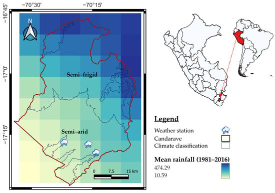
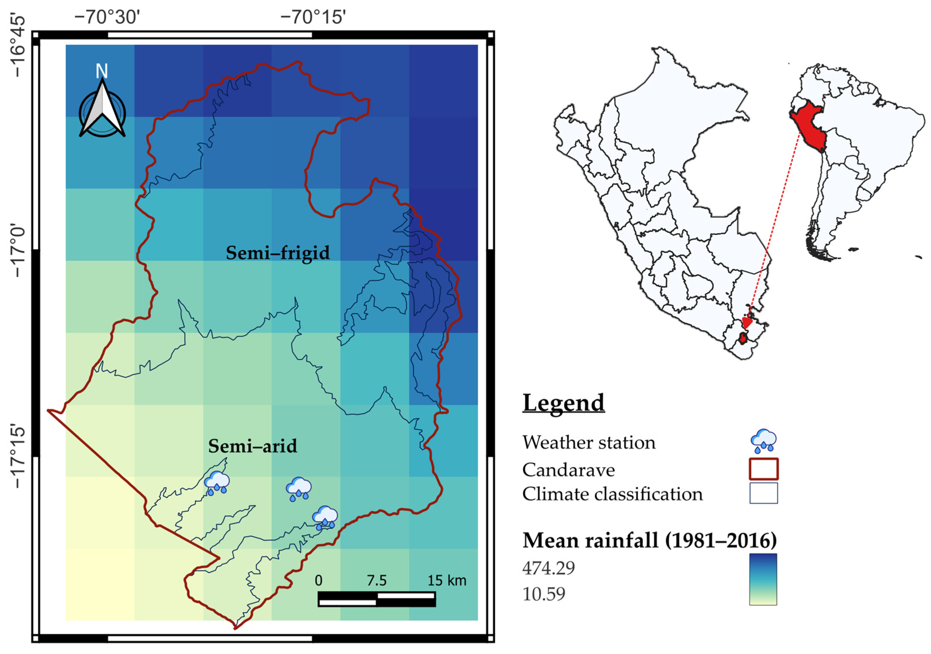
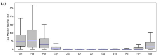
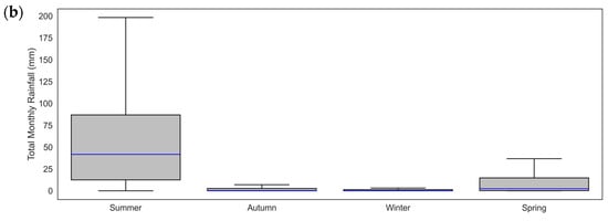
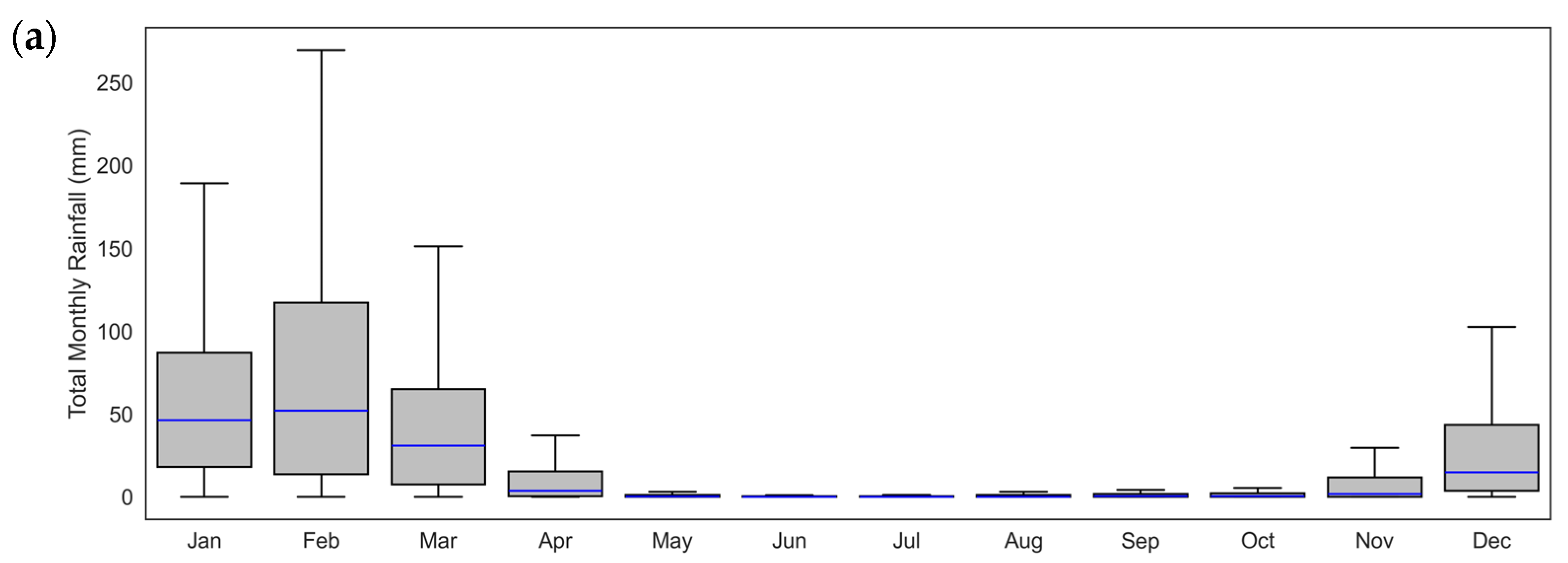
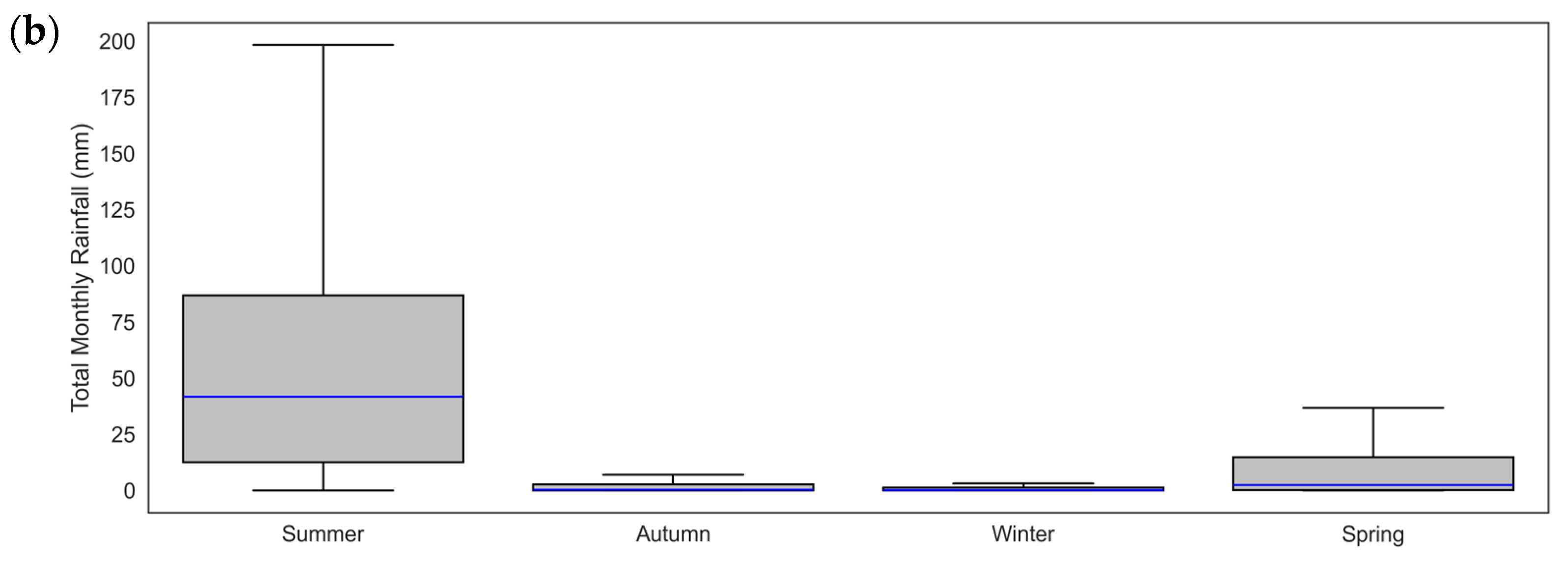
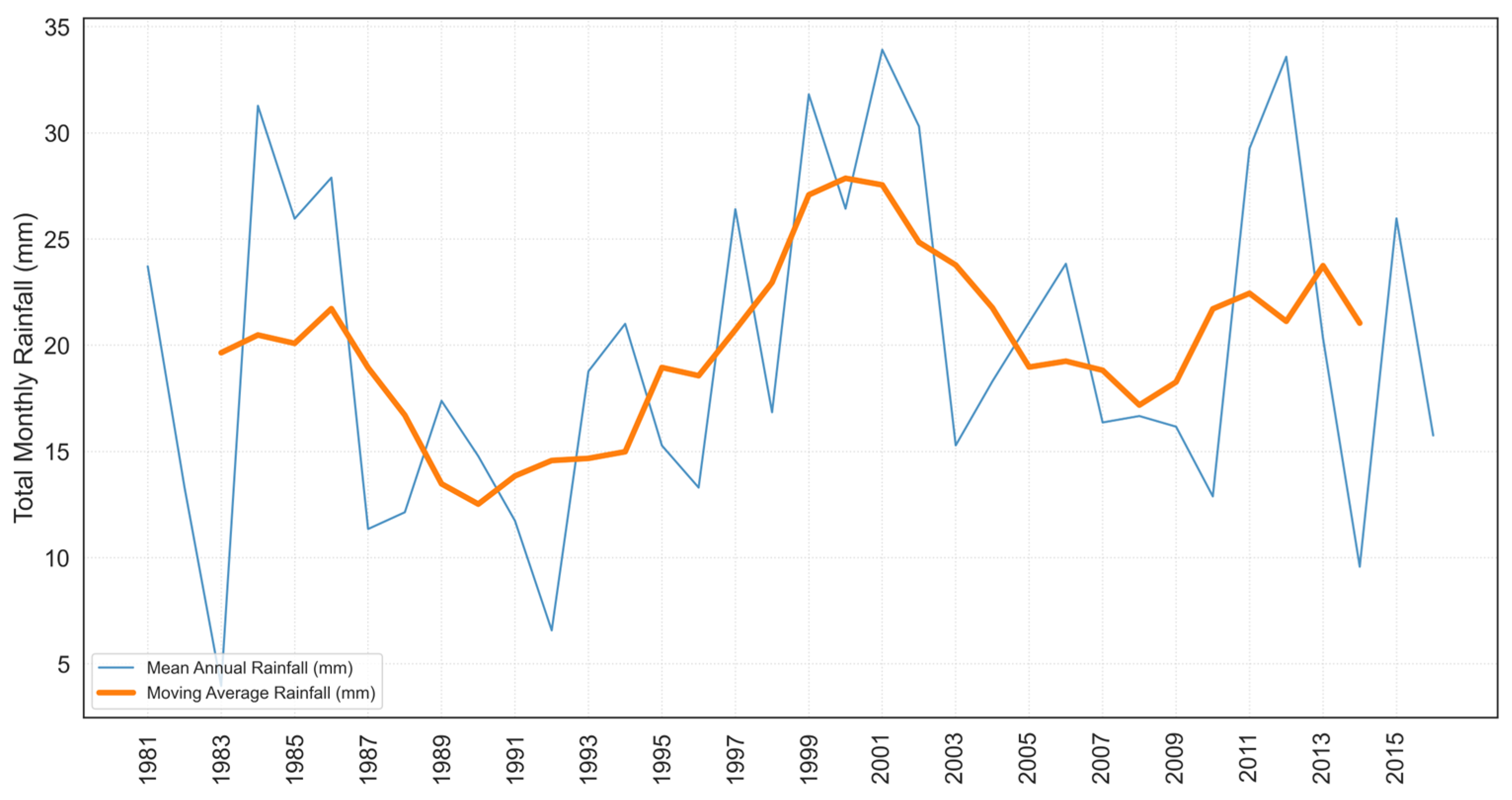
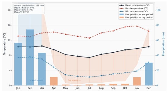
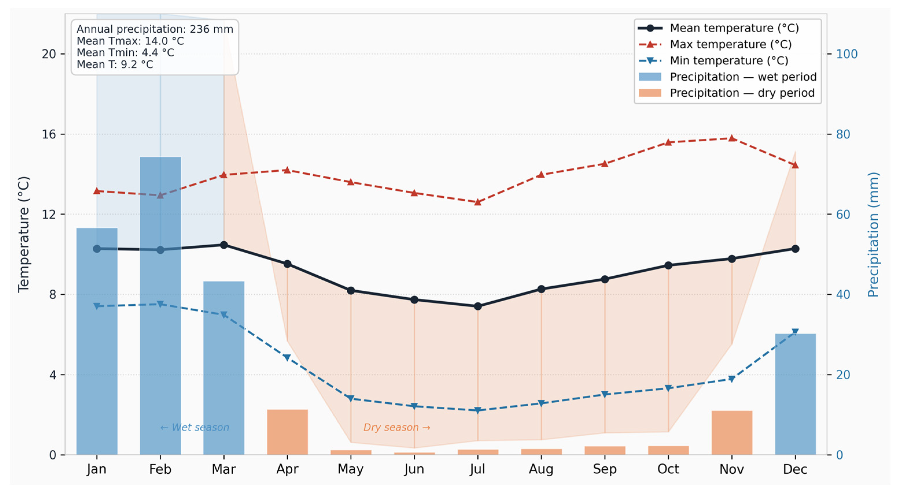
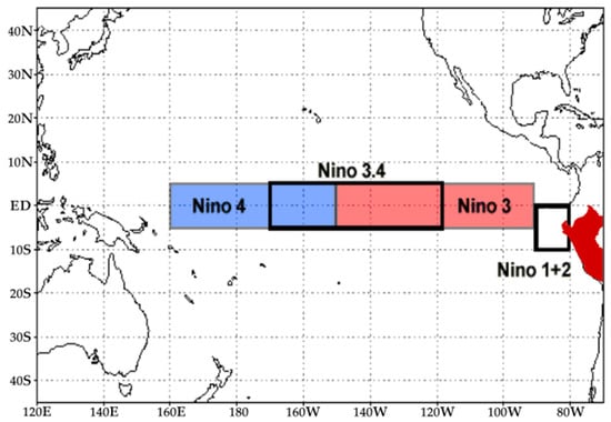
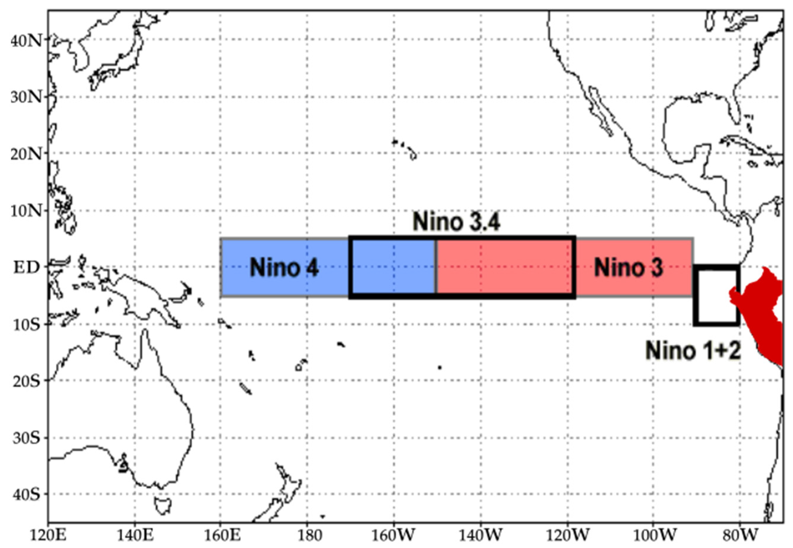
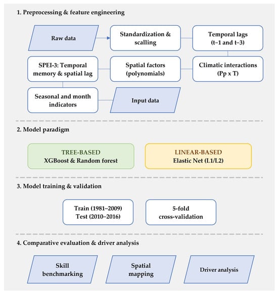
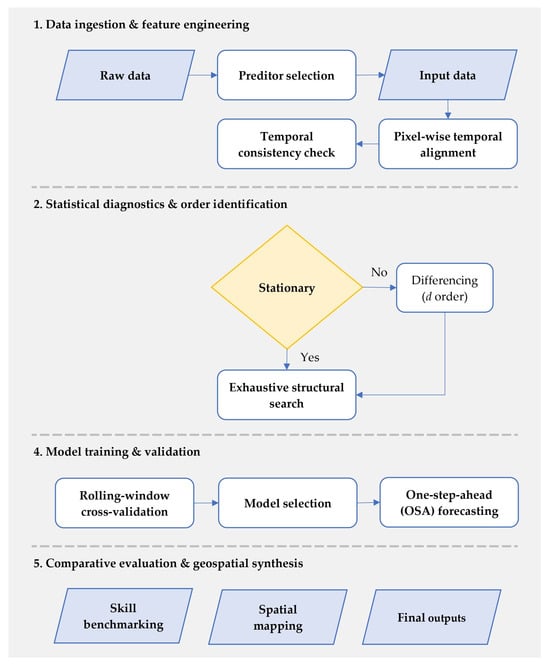
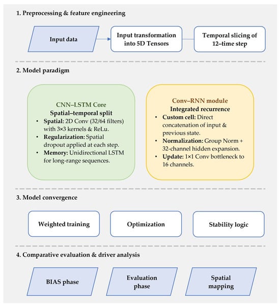
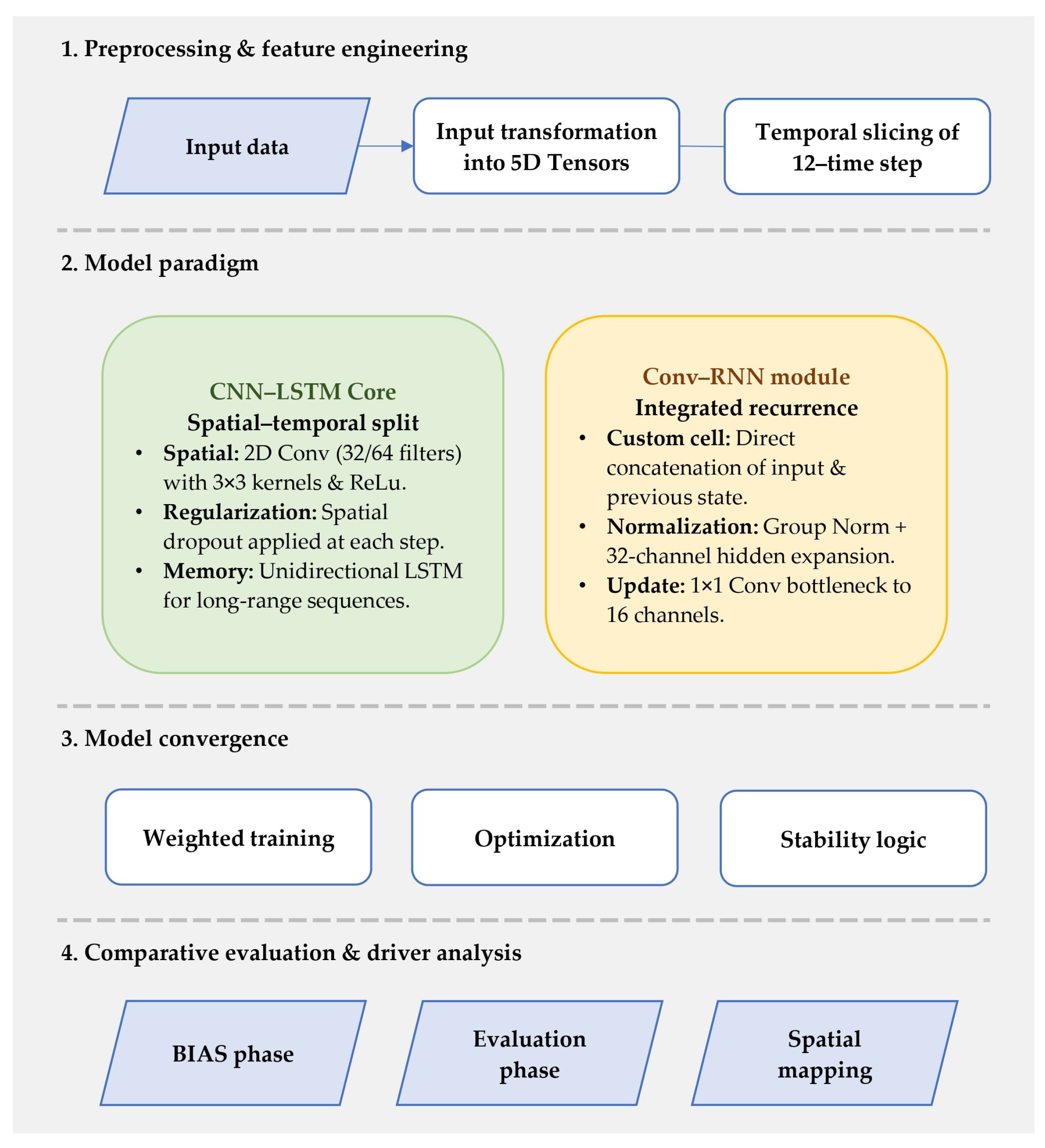
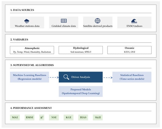
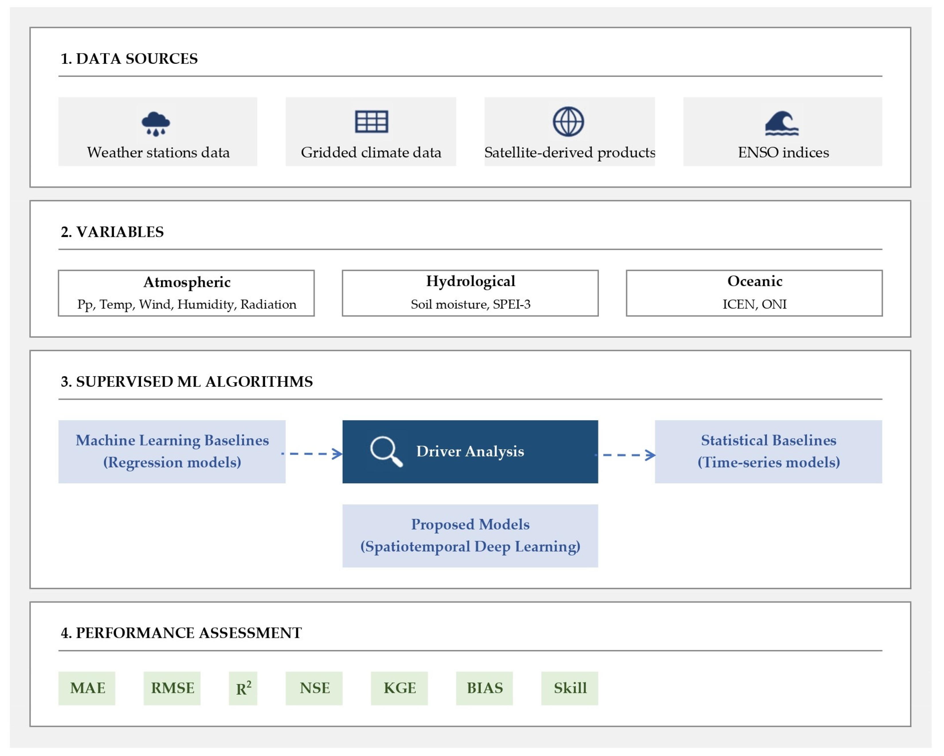
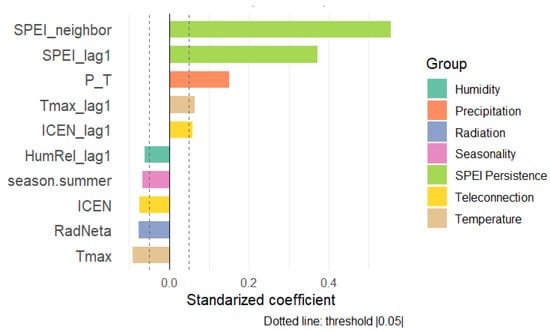
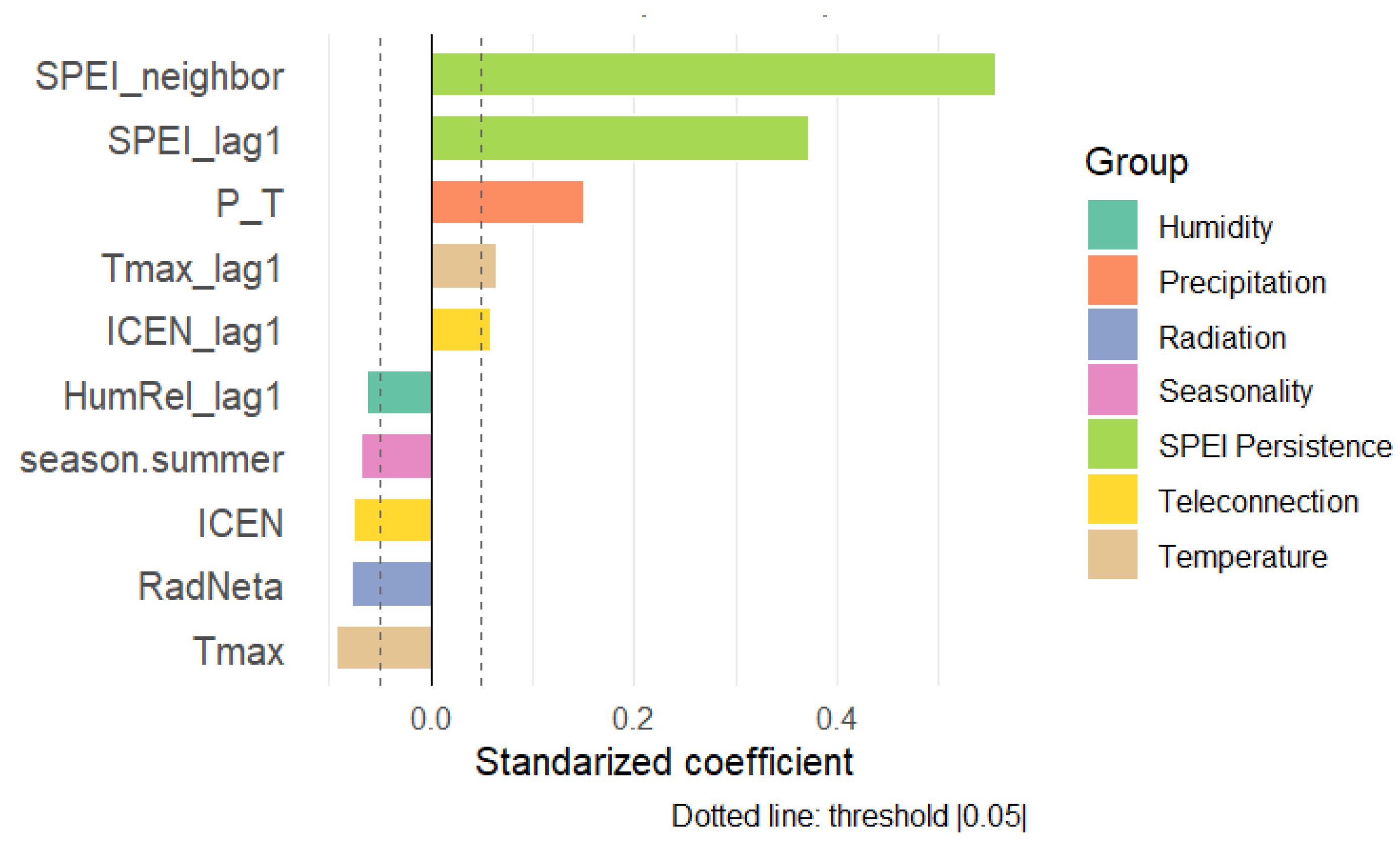
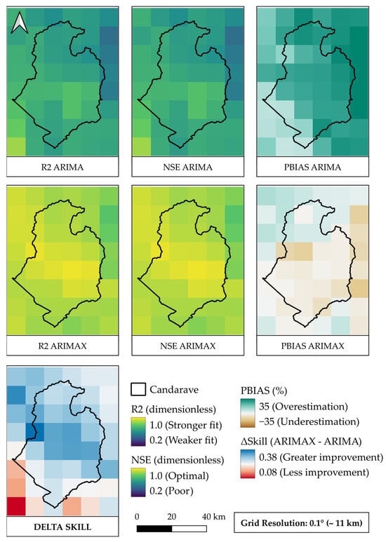
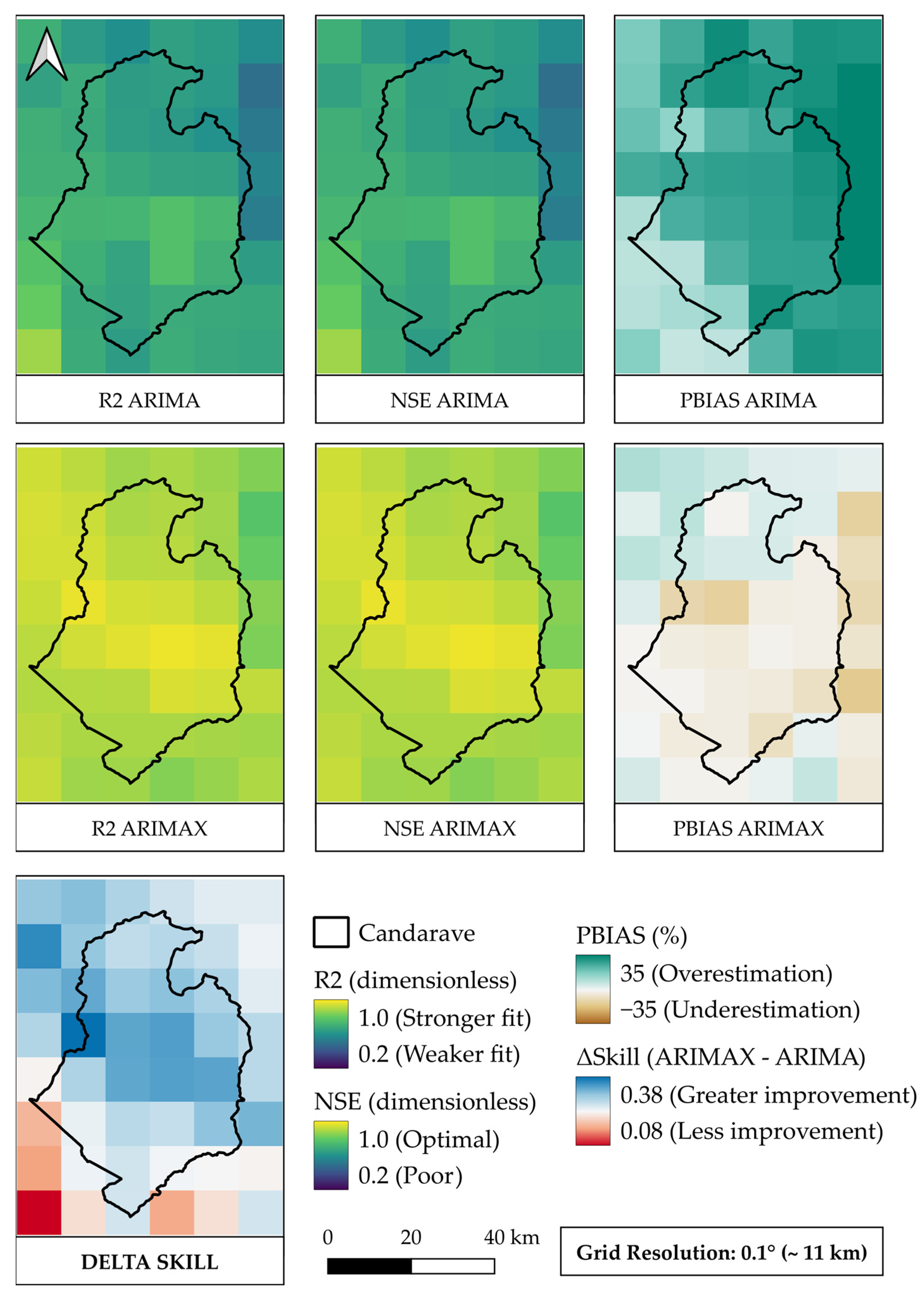
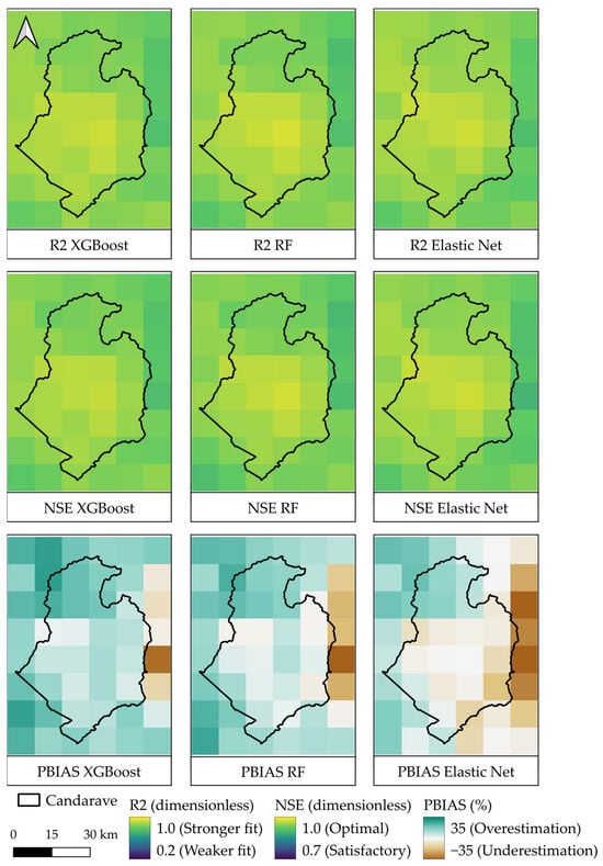
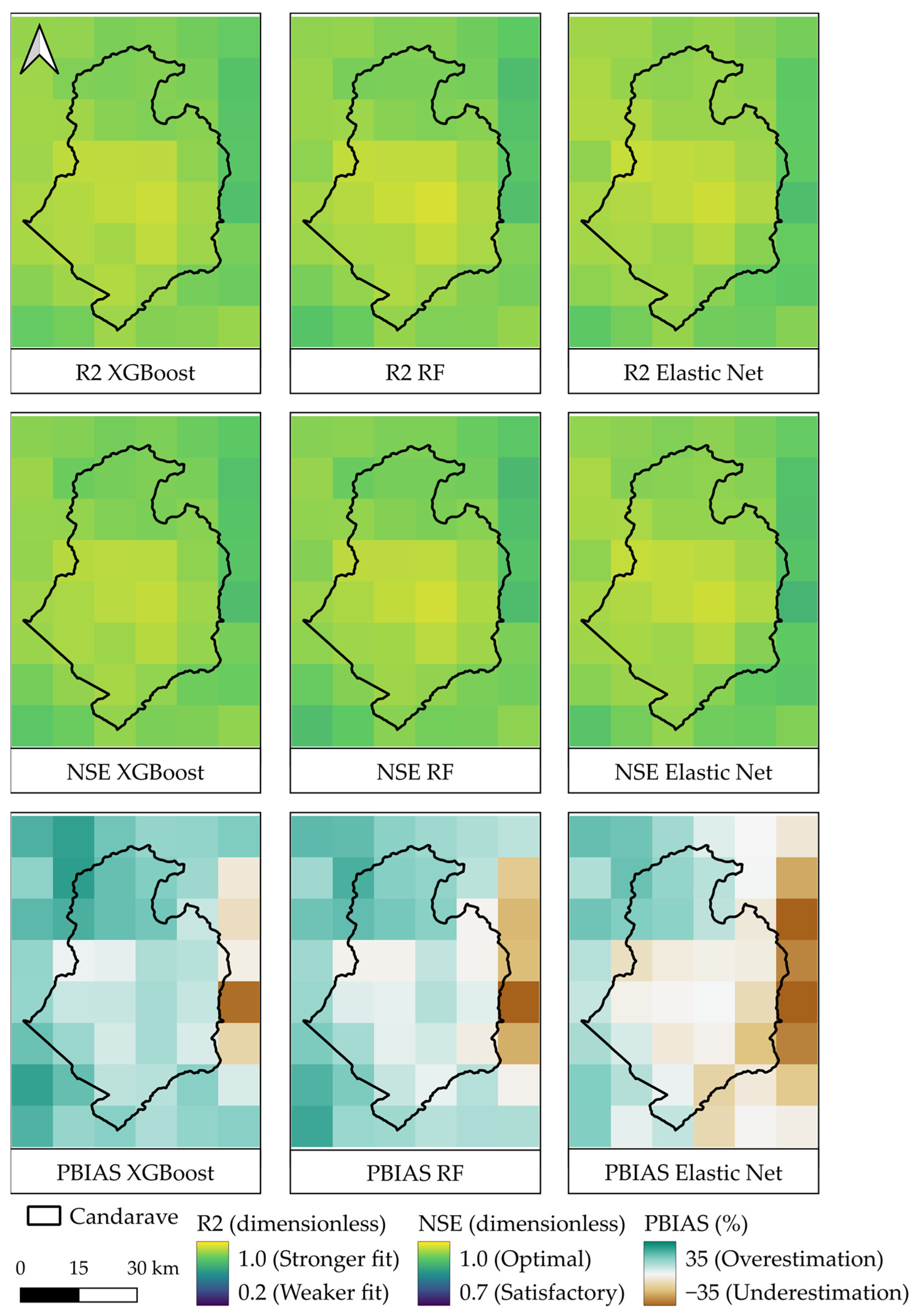
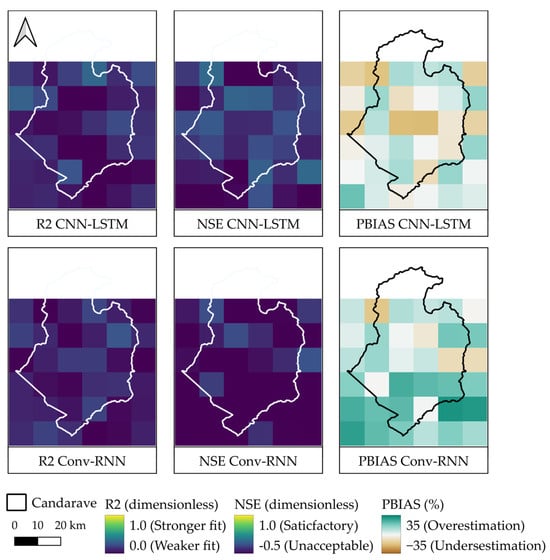
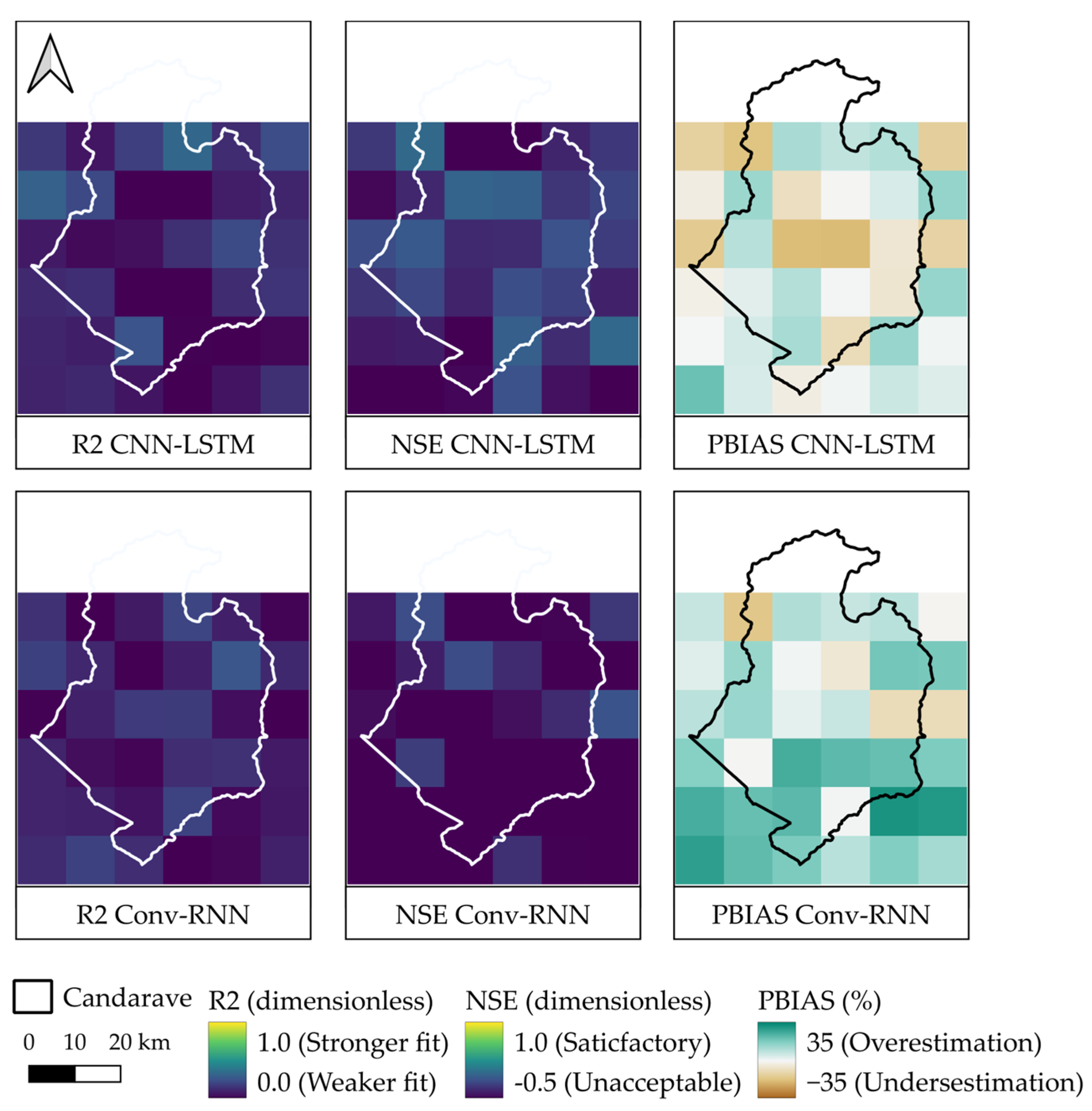
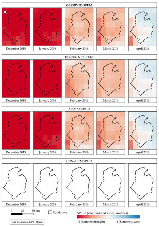
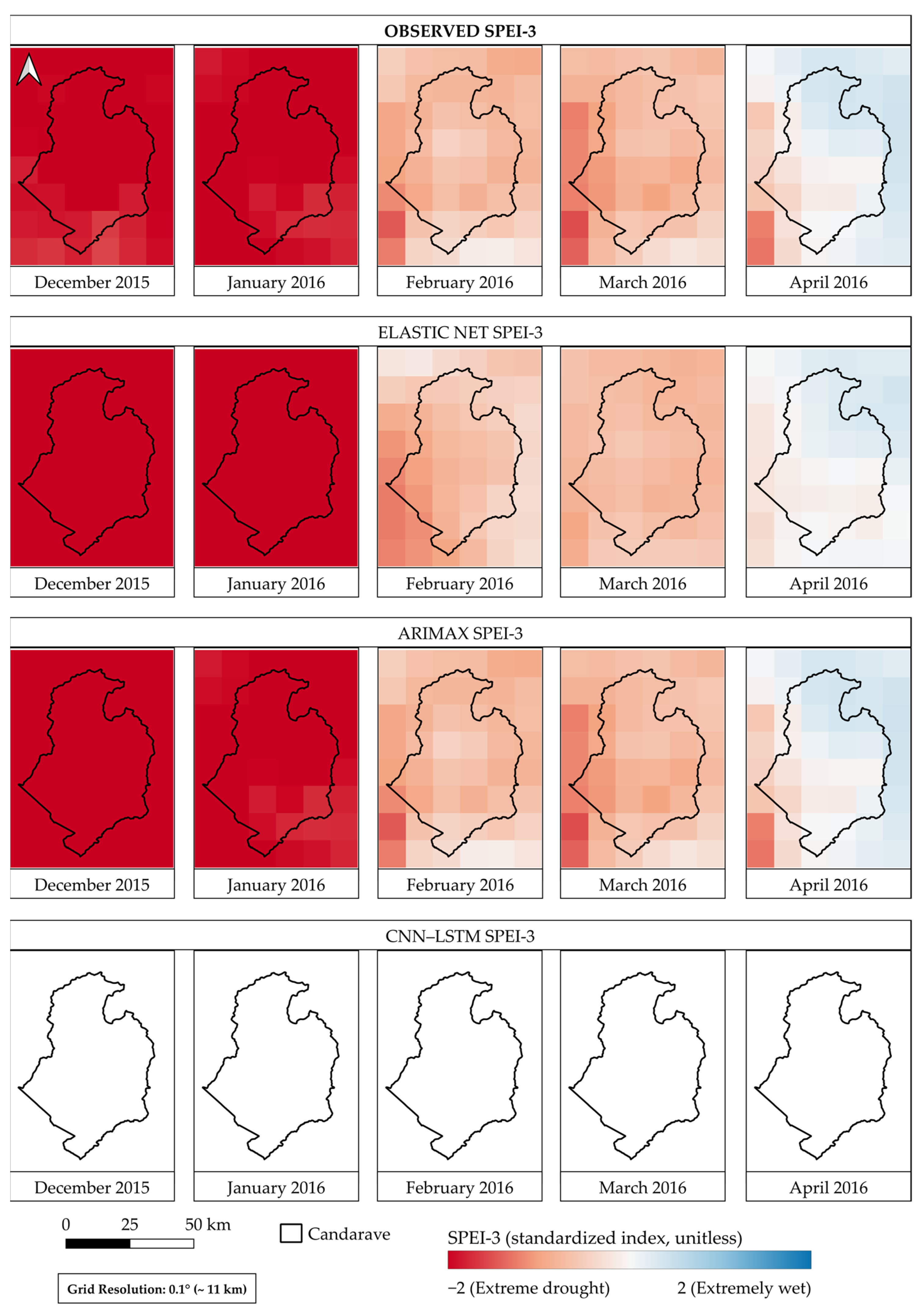

Disclaimer/Publisher’s Note: The statements, opinions and data contained in all publications are solely those of the individual author(s) and contributor(s) and not of MDPI and/or the editor(s). MDPI and/or the editor(s) disclaim responsibility for any injury to people or property resulting from any ideas, methods, instructions or products referred to in the content. |
© 2026 by the authors. Licensee MDPI, Basel, Switzerland. This article is an open access article distributed under the terms and conditions of the Creative Commons Attribution (CC BY) license.