


Abstract
HI35, defined as the mean annual number of days on which apparent temperature exceeds 35 °C, is introduced in this paper as a country-level heat exposure metric. Unlike vulnerability indicators, HI35 is treated as an exogenous climatic exposure variable and not as a direct measure of vulnerability or as an endogenous outcome. By combining HI35 with World Bank Environmental, Social, and Governance (ESG) indicators, this study applies unsupervised clustering algorithms to derive an exposure–vulnerability typology of countries. The Environmental, Social, and Governance pillars are analyzed separately through dedicated clustering procedures, supported by robustness checks and an additional country taxonomy based on principal component analysis and hierarchical clustering. The results identify heterogeneous country profiles in which similar levels of heat exposure coexist with different ESG-based vulnerability conditions, including environmental pressures, fragility, institutional capacity, innovation, water access, nutrition, and governance quality. Conversely, countries with relatively low heat exposure may display differentiated social or institutional vulnerability profiles. The empirical evidence suggests that heat exposure and ESG-based vulnerability are conceptually distinct but jointly relevant dimensions for classifying climate-risk profiles. No causal relationship is inferred between ESG indicators and HI35; the analysis is descriptive, classificatory, and based on unsupervised learning. Conceptually, HI35 captures the occurrence of extreme heat events, while ESG indicators describe the environmental, social, and institutional conditions associated with sensitivity, resilience, and adaptive capacity.
1. Introduction
Climate change is a systemic phenomenon, and ESG factors have gained importance as a framework for examining the environmental, social, and institutional conditions under which societies face climatic stress [1]. In this research, we consider HI35, defined as the annual number of days on which apparent temperature exceeds 35 °C. HI35 reflects heat exposure and is not treated as a proxy for a country’s vulnerability to climate change. Countries with similar levels of heat exposure may display different ESG-based vulnerability profiles, depending on environmental pressures, societal sensitivity, institutional quality, and adaptive capacity. Therefore, the research question of this paper is as follows: how can HI35 and ESG indicators be jointly used to differentiate country-level exposure–vulnerability profiles? From a methodological perspective, we apply cluster analysis to an integrated country-level dataset including HI35 and ESG indicators. The method is descriptive and classificatory in nature, as it aims to identify groups of countries with similar heat-exposure conditions and ESG-based vulnerability-related profiles. No causal relationship is inferred between ESG indicators and HI35. The twofold contribution of the research is, first, to advance the classification of climate-risk profiles by jointly considering climatic exposure and the socio-institutional conditions under which exposure occurs. Second, the study shifts attention from firm-level ESG performance to cross-country ESG-based vulnerability profiles, an area that remains underexplored in the climate-risk literature.
This paper is structured as follows. Section 2 reviews the literature on ESG, heat exposure, and climate vulnerability. Section 3 presents the data, variables, aggregation procedure, cleaning strategy, and country-level unit of analysis. Section 4 explains the empirical framework, distinguishing HI35 as climatic exposure from ESG-based vulnerability. Section 5, Section 6, Section 7 and Section 8 report the clustering results for the Environmental, Social, and Governance dimensions, including sensitivity analyses and robustness checks. Section 9 develops an integrated country taxonomy using PCA and hierarchical clustering, with macroeconomic and institutional interpretation. Section 10 discusses the empirical findings, while Section 11 derives policy implications for climate governance and heat resilience. Section 12 concludes this paper. Appendix A, Appendix B and Appendix C provide descriptive statistics and diagnostics for Environmental, Social, and Governance indicators. Appendix D reports long-term HI35 trends from 2000 to 2022.
2. Literature Review
Extreme heat events are becoming more prevalent, prompting policymakers, investors, and academics to reconsider how sustainability and climate risks are assessed. HI35, defined as the annual number of days on which apparent temperature exceeds 35 °C, is used in this study as an indicator of climatic heat exposure. However, HI35 is not treated as a direct vulnerability metric. The key challenge of the analysis is to understand how this exogenous exposure variable is associated with environmental, social, and governance conditions that describe vulnerability-related country profiles, without implying any causal relationship between ESG indicators and HI35.
Previous research shows a positive link between ESG performance and resilience to heat stress. The bulk of available literature focuses on individual companies or industrial sectors. Refs. [2,3] found that Chinese firms with higher ESG ratings showed greater resilience, as evidenced by lower volatility during extreme heat. At the same time, studies by [4,5] highlight the importance of ESG-based actions in reducing the impacts of heat exposure on economies. Nonetheless, the existing literature has failed to shed light on how ESG systems function as national vulnerability structures.
A similar strand of academic discourse explores reliability issues of ESG and climate exposure metrics. For instance, Refs. [6,7] suggest that ESG indicators might lose validity and consistency without solid institutional and data structures. Refs. [8,9,10] highlight the benefits of HI35 and similar indicators for sustainability planning and institutional ESG structures. Still, exposure indicators are inconsistently used in ESGs, and discrepancies between ESG data providers can lead to different interpretations of climate risks [11,12,13].
Moreover, the social and governance sides of heat vulnerability are understudied. Extreme temperatures cause severe health outcomes, impact workers’ productivity, alter nutrition, exacerbate inequality, hinder access to public utilities, and contribute to migration. However, these risks are frequently neglected when evaluating ESG factors [14,15,16,17,18]. Similarly, the influence of governance on adaptive capacity, regulatory coordination, and climate-risk management requires further analysis since there is currently no comparative analysis of institutional profiles across countries at different heat exposures [19,20,21,22,23,24,25].
Innovation and data infrastructure also play important roles. Both ESG investments and R&D can improve adaptation, especially when they concern energy and technological sectors [26,27,28,29,30,31]. At the same time, reliable ESG data, geospatial information, and comparability become necessary for climate-risk assessment [7,32,33,34].
This paper addresses the following four gaps: (i) the prevalence of firm- or sector-level analyses; (ii) the patchy use of heat indicators in ESG frameworks; (iii) the lack of operationalized social and governance vulnerability indicators; and (iv) the absence of systematic cross-country taxonomies. In particular, the author uses HI35 and other ESG indicators in a joint analysis with machine learning techniques. Thus, exposure–vulnerability clusters are described without assuming causality. See Table 1.
Table 1.
Synthesis of the literature review.
Despite being originally designed as an instrument for assessing sustainability and risk in corporate investments, the extension of ESG to the analysis of national characteristics requires re-conceptualizing the theory [41,42]. This paper does not consider the ESG framework as a measure of corporate sustainability, nor as a national ranking based on firm-level assessment principles. Rather, ESG is regarded as a macro-sustainability approach for describing nation-specific conditions associated with vulnerability-related profiles and adaptive capacity under exogenous climatic exposure [43,44]. Thus, the three main components of the ESG concept are considered as structural dimensions through which country-level climate vulnerability profiles can be classified. Specifically, the environmental pillar includes ecological pressures, depletion of natural resources, energy dependence, greenhouse gas emissions, and cooling stresses. The social pillar concerns population sensitivity to health, nutrition, demographics, and the provision of basic service parameters. Finally, the governance pillar accounts for issues of regulatory quality, rule of law, political stability, accountability, human rights protection, innovation capability, and the overall state of macroeconomic governance [43,44]. Clearly, the above taxonomy does not intend to create an all-inclusive development index but rather defines the boundaries within which national conditions associated with climate vulnerability are analyzed. HI35 is viewed as an exogenous index of climatic exposure, while the ESG variables represent national characteristics associated with sensitivity, resilience, and adaptive capacity under climate exposure [44]. GDP growth is used because it is contained in the World Bank database and viewed as an element of macroeconomic governance. Future development of the taxonomy should be focused on GDP per capita, income groups, fiscal capacity, and urbanization factors [43,44].
3. Data Architecture and Variable Framework
We have used the following data from the World Bank Database (Table 2).
Table 2.
Variables used to construct the HI35–ESG exposure–vulnerability framework.
The countries (Afghanistan, Albania, Algeria, Angola, Argentina, Armenia, Australia, Austria, Azerbaijan, Bahrain, Bangladesh, Barbados, Belarus, Belgium, Belize, Benin, Bhutan, Bolivia, Bosnia and Herzegovina, Botswana, Brazil, Bulgaria, Burkina Faso, Burundi, Cambodia, Cameroon, Canada, Central African Republic, Chad, Chile, China, Colombia, Congo Dem. Rep., Congo Rep., Costa Rica, Cote d’Ivoire, Croatia, Cuba, Cyprus, Czechia, Denmark, Djibouti, Dominica, Ecuador, Egypt Arab Rep., El Salvador, Equatorial Guinea, Eritrea, Estonia, Eswatini, Ethiopia, Fiji, Finland, France, Gabon, Gambia The, Georgia, Germany, Ghana, Greece, Grenada, Guatemala, Guinea, Guinea-Bissau, Guyana, Haiti, Honduras, Hungary, Iceland, India, Indonesia, Iran Islamic Rep., Iraq, Ireland, Israel, Italy, Jamaica, Japan, Jordan, Kazakhstan, Kenya, Kiribati, Korea Dem. People’s Rep., Kuwait, Kyrgyz Republic, Lao PDR, Latvia, Lebanon, Lesotho, Liberia, Libya, Liechtenstein, Lithuania, Luxembourg, Madagascar, Malawi, Malaysia, Maldives, Mali, Malta, Marshall Islands, Mauritania, Mauritius, Mexico, Micronesia Fed. Sts., Moldova, Monaco, Mongolia, Montenegro, Morocco, Mozambique, Myanmar, Namibia, Nauru, Nepal, Netherlands, New Zealand, Nicaragua, Niger, Nigeria, North Macedonia, Norway, Oman, Pakistan, Palau, Panama, Papua New Guinea, Paraguay, Peru, Philippines, Poland, Portugal, Qatar, Romania, Russian Federation, Rwanda, Samoa, San Marino, Sao Tome and Principe, Saudi Arabia, Senegal, Serbia, Seychelles, Sierra Leone, Singapore, Slovak Republic, Slovenia, Solomon Islands, Somalia, South Africa, South Sudan, Spain, Sri Lanka, St. Kitts and Nevis, St. Lucia, St. Vincent and the Grenadines, Sudan, Suriname, Sweden, Switzerland, Syrian Arab Republic, Tajikistan, Tanzania, Thailand, Timor-Leste, Togo, Tonga, Trinidad and Tobago, Tunisia, Turkiye, Turkmenistan, Tuvalu, Uganda, Ukraine, United Arab Emirates, United Kingdom, United States, Uruguay, Uzbekistan, Vanuatu, Venezuela RB, Viet Nam, Yemen Rep., Zambia, Zimbabwe.) included in this analysis are represented in the following map. Data cover the period from 1999 to 2023. See Figure 1.
Figure 1.
Geographic Distribution of Countries Included in the ESG–HI35 Analysis. Note. The figure displays countries included in the ESG–HI35 dataset used for clustering analysis. Selected countries cover the 1999–2023 period and represent diverse climatic, environmental, social, and governance conditions worldwide.
3.1. Temporal Scope and Aggregation Procedure
The data come from the World Bank ESG database and consist of yearly observations of all indicators for each country, over the longest available period for each indicator. Given the imbalance in data availability over time and space, we use an unbalanced panel [45,46]. To conduct clustering, we take the annual mean to form cross-sectional data at the country level. That is, for each country and each indicator, we aggregate annual observations by averaging them, resulting in one average value per country for HI35 and ESG indicators. The use of the mean was justified, as our research aims to identify countries’ long-run exposure and vulnerability profiles rather than year-by-year dynamics or fluctuations. Observations with missing values, as well as outliers that will be identified during plausibility testing conducted next, will not be included when forming country means. As a result, country-level means will be computed only from valid values. Thus, after temporal aggregation, we end up with a set of observations, where each country is characterized by a single observation that includes its long-run HI35 mean and ESG variables. Therefore, our clusters should be viewed as long-run exposure and vulnerability profiles at the country level [45,47]. Additional information on the temporal variation in countries’ HI35 values will be presented in Appendix D. The time series themselves will not be used in clustering algorithms, but they will provide insight into long-run heat exposure variation [46].
3.2. Data Cleaning and Plausibility Checks
Before conducting temporal aggregation and clustering, a structured data-cleaning and plausibility-check procedure was implemented to identify physically impossible observations, coding errors, missing records, and inconsistencies in indicator scales. This screening was conducted separately for each variable used in the analysis because all environmental, social, governance, and HI35 indicators have physically and/or conceptually admissible ranges. For indicators with upper and lower bounds, admissible ranges were defined according to each indicator’s substantive meaning and measurement scale. Percentage indicators were checked for physical feasibility, while counts, rates, and index variables were assessed to detect negative values, out-of-range records, or implausible observations. Missing observations, physically impossible values, and inconsistent records were not imputed before clustering; instead, they were excluded from the computation of country-level means. As a result, temporal aggregation was based only on valid observations, reducing the risk that data anomalies would distort the construction of long-run exposure–vulnerability profiles.
3.3. Unit of Analysis and Aggregation Rationale
For the present investigation, countries are used as the unit of analysis to develop a cross-national typology of exposure and vulnerability situations based on ESG scores [43,47]. This choice reflects the nature of the World Bank ESG database, which computes environmental, social, governance, and HI35 indicators at the country level. Using countries as the unit of analysis will enable cross-national comparisons and facilitate comparisons of institutional capacity, public service provision, environmental pressure, and national resilience within a unified metric system [44,45].
Analytically speaking, using countries as the unit of analysis is quite relevant for several reasons. Many of the ESG dimensions discussed above are defined primarily in terms of national policies and institutions. Thus, the quality of governance, institutional capacity, rights and freedoms, stability, research support, public healthcare systems, social provisions, and environmental management are largely national phenomena [43,45]. As a result, using a country as the unit of analysis enables researchers to identify exposures and vulnerabilities that are essential for national adaptation efforts and ESG assessments [44,47].
At the same time, this choice entails some limitations. First, each country exhibits some degree of heterogeneity, and using country averages as the unit of analysis may ignore relevant subnational variation. In particular, this problem becomes especially acute when it comes to very big and diverse countries like China, the US, India, and Brazil, where various climate zones exist alongside one another and where urbanization, infrastructure development, institutional capacity, social vulnerability, and climatic exposure may vary significantly across a single nation [44].
Thus, in this regard, the study’s findings cannot be interpreted as a map of heat risks [44]. Instead, it is supposed to deliver a typology of countries according to their exposure–vulnerability relations [43,47]. While using a country as the unit of analysis may be appropriate for cross-national comparisons of national indicators of ESG and exposures, it is associated with aggregation problems that may mask subnational variation in exposure and vulnerability to heat. Future investigations will need to develop methods to measure the impacts of heat risk within metropolitan regions [44,45].
4. Empirical Framework and Methodological Rationale: Classifying ESG–Heat Exposure Vulnerability Profiles
This section presents the empirical framework used to construct the ESG–HI35 exposure–vulnerability taxonomy. The framework clarifies how climatic exposure and ESG-based vulnerability are analyzed together while remaining conceptually distinct. HI35 is treated as an exogenous climatic exposure indicator, not as a direct measure of vulnerability. ESG variables are used to describe environmental, social, and governance-related conditions associated with sensitivity, resilience, and adaptive capacity. The section also explains the clustering strategy and the boundary conditions for interpreting the resulting taxonomy. The clustering analysis is applied to the temporally aggregated country-level dataset described in previous sections. Therefore, the empirical framework does not model year-by-year variation, dynamic temporal relationships, or panel effects. Instead, it classifies countries according to their long-run average combinations of climatic exposure and ESG-based vulnerability conditions. No parametric regression models are estimated in this study. Accordingly, no variable is specified as dependent or independent in an econometric sense. HI35 is included in the clustering space as an exogenous climatic exposure indicator. ESG variables are included as descriptors of environmental, social, and governance-related vulnerability and adaptive-capacity conditions. The analysis is therefore entirely unsupervised and cluster-based.
4.1. Distinguishing Climatic Exposure from ESG-Based Vulnerability
The methodological framework is designed with a clear separation between climatic exposure and vulnerability. Specifically, the ESG approach is first broken down into its three essential pillars: Environment, Society, and Governance. This framework allows the identification of institutional, social, and environmental conditions associated with vulnerability and adaptability to high temperatures. According to the research conceptual framework, HI35 is neither a measure of vulnerability nor a vulnerability outcome. Indeed, HI35 is an external measure of climatic exposure, reflecting the number of days when apparent temperature exceeds 35 degrees centigrade [48,49].
Vulnerability is defined as the interaction between exposure, sensitivity, and adaptive capacity. As a result, ESG variables can help identify the institutional and structural factors that affect nations’ vulnerability and adaptation to extreme heat. The methodological framework will include the definition of two levels of exposure: climatic exposure, represented by HI35 and determined primarily by geographical and atmospheric factors; and systemic vulnerability, which can be measured through various ESG variables, such as environmental pressures, social vulnerabilities, institutional quality, and governmental capacity. ESG indicators cannot be used as factors determining the existence of the HI35 phenomenon; nor can they be considered explanatory of its occurrence.
Secondly, the research will rely on different unsupervised clustering models to detect the emergence of configurations involving both HI35 and ESG. Specifically, a variety of models will be analyzed: Density-Based clustering, Fuzzy C-Means, Hierarchical clustering, Model-Based clustering, K-Means, and Random Forests Proximity clustering. Different measures will be used to evaluate model quality, including R2, silhouette scores, the Calinski–Harabasz ratio, AIC, BIC, and entropy criteria. Given the unsupervised nature of clustering, models will be selected based on statistical performance, geographical spread, cluster balance, semantic meaning, and clarity of exposure–vulnerability regimes [50].
Thirdly, after technical classification, the taxonomy of exposure–vulnerability regimes will be established based on the identified clusters. Clusters will be interpreted as specific exposure–vulnerability regimes combining different features of exposure (HI35) and socio-institutional structures. In other words, the analysis will demonstrate that countries with the same climatic exposure can exhibit different vulnerabilities due to their environmental, social, and institutional conditions. Therefore, the regime taxonomy will not state the causal relationship between HI35 exposure and ESG structures, but will show how countries differ in terms of adaptive capacity.
The research methodology uses a descriptive, classificatory approach. Namely, this study will analyze the pattern of co-variation between HI35 and ESG indicators to classify countries into clusters. Such an approach will avoid any causal inference and treat HI35 as independent of ESG measures. ESG indicators will include resource depletion, population pressure, innovation capacity, institutional quality, and governance efficiency.
In conclusion, the methodology proposed in this paper provides a systematic approach to examining climatic exposure and systemic vulnerability. Specifically, the methodology explains that HI35 reflects exposure to heat, while ESG variables capture the environmental, social, and institutional structures that determine the extent to which nations may be vulnerable to extreme climate conditions.
4.2. Boundary Conditions and Scope of Applicability
This classification needs to be understood within clear boundary conditions. This is applicable to macro-level comparative analyses, such as comparing countries, benchmarking countries’ sustainability, conducting international climate risk assessments, and assessing national adaptations to climate change, but not for local heat risk mapping [43,47]. The outcomes will depend on the selected indicators, the World Bank ESG dataset framework, the timespan, and the method used to perform the cluster analysis; using other datasets or geographical units could yield different vulnerability clusters [43,44]. The classification is only descriptive and used to categorize exposure–vulnerability clusters.
5. Clustering Framework and Empirical Results
Building on the exposure–vulnerability framework presented in Section 4, this section reports the clustering results for the Environmental, Social, and Governance dimensions. HI35 is used as the climatic exposure indicator, while ESG variables represent socio-institutional and environmental conditions related to sensitivity, resilience, and adaptive capacity. The analysis identifies groups of countries characterized by different combinations of heat exposure and ESG-based vulnerability. Since the indicators are temporally averaged at country level, the clusters should be interpreted as structural classifications rather than year-specific outcomes or temporal trajectories.
Three separate clustering analyses were conducted, one for each ESG pillar. In each case, countries were grouped according to their ESG characteristics and corresponding HI35 values. This strategy allows the identification of exposure–vulnerability configurations and comparison of countries that may experience similar climatic exposure but differ in environmental fragility, social sensitivity, health-related conditions, institutional quality, or governance capacity.
Six unsupervised clustering algorithms were applied to each ESG dimension: Density-Based, Fuzzy C-Means, Hierarchical, Model-Based, K-Means, and Random Forest proximity clustering [51,52,53]. Algorithm performance was evaluated through a multi-metric framework combining clustering quality, parsimony, and interpretability. R2, Silhouette, and Calinski–Harabasz scores were maximized, while AIC, BIC, and entropy were minimized. All indicators were normalized using Min–Max scaling, with inversion applied to minimization metrics to ensure comparability.
Using multiple algorithms strengthens robustness by reducing method-specific bias, since different approaches rely on different assumptions about cluster shape, density, variance, and distance structure. However, model selection was not based mechanically on a single metric. The final choice combined statistical performance, cluster balance, substantive interpretability, and coherence with the exposure–vulnerability framework. Solutions with high internal validity but highly unbalanced clusters were not preferred, as they offered limited value for constructing an interpretable country taxonomy.
Although the same selection protocol was applied across all ESG pillars, the preferred algorithm may differ because each dataset has distinct statistical properties. The procedure therefore followed the same sequence: exclusion of degenerate solutions, comparison of normalized metrics, assessment of cluster-size balance through the HH index, and final evaluation of interpretability. Cluster means were computed using the original, non-standardized variables and are reported in their original scales. Additional diagnostics are provided in Appendix A, Appendix B and Appendix C.
6. Comparative Evaluation of Clustering Algorithms for the Environmental Dimension
The chosen clustering algorithm is K-Means, as it provides the best performance across all criteria, including balance between statistics, interpretation, parsimony, and cluster size [54,55]. Even though the best Silhouette of 0.84 can be reached in Density-Based clustering, along with high Pearson’s γ and low entropy, the method fails to generate a solution that would be considered balanced. The number of clusters is large, yet nearly all observations cluster into one large cluster, with a few others containing only a few objects. As a result, the HH Index is very high (0.9734), with 16 noise points identified. Therefore, this method cannot be used for interpretative taxonomy [56,57]. Hierarchical clustering shows good results on some metrics (R2, Silhouette, max diameter), but it is not balanced, as the observations mostly cluster into a single large cluster. As a result, the HH Index value is quite high—0.9149 [56,58]. At the same time, K-Means achieves the best R2 (0.804), CH index, and the lowest AIC and BIC. The Silhouette is positive, and the HH Index equals 0.1881, meaning that the algorithm generates a more diverse cluster structure. See Table 3.
Table 3.
Comparative Performance of Clustering Algorithms for the Environmental Dimension.
A total of ten different cluster configurations of environmental variables were identified through the analysis. All variables are reported using their original measurement scales. As such, HI35 refers to the average number of days per year when the temperature exceeds 35 °C, and the ESG variables refer to their own unit of [44,47]. Clusters 1 and 2 display low-to-medium profiles. In particular, Cluster 1 shows a negative NFD value and other environmental variables close to zero. Cluster 2 shows similar characteristics, with an increased NRD value and negative ME and N2O values. Cluster 3 is characterized by an intermediate profile, as indicated by positive NRD and NFD values and negative ME and N2O values [43,45]. Cluster 4 shows a highly unusual profile, characterized by very high values of HI35, EIN, EIL, FFEC, and ME and negative NFD and N2O values. The high structural density of this cluster is indicative of a high-intensity environment or productive structure, but it does not correlate with increased N2O emissions. In turn, Cluster 5 is primarily represented by HI35, which has the highest value in the dataset. Positive values are recorded for EIL and ME, while neither EIN nor FFEC is significantly increased [44,47]. Cluster 6 shows a very low NRD but high N2O, indicating a very critical environmental profile marked by a serious depletion of resources coupled with emissions stress [59,60]. In contrast, Cluster 7 appears better, with positive NRD and NFD and negative ME and N2O values. Cluster 8 combines positive NFD and EIL together with positive N2O. Cluster 9 features negative NFD, high ME, and N2O [46,61]. Finally, Cluster 10 is characterized by the highest EIL, with moderate values for the other variables. In summary, clusters 4, 5, and 6 seem the most extreme clusters, while clusters 3, 7, and 10 represent a relatively balanced cluster profile. See Table 4.
Table 4.
Environmental Cluster Profiles Based on HI35 and ESG Indicators.
Figure 2 reports the Silhouette plot associated with the Environmental K-Means clustering solution. The graph provides an assessment of cluster cohesion and separation by measuring the Silhouette coefficient for each observation across the ten identified environmental clusters. Positive Silhouette values indicate that observations are, on average, more similar to members of their own cluster than to observations belonging to neighboring clusters, thus supporting the internal consistency of the environmental taxonomy. See Figure 2.
Figure 2.
Silhouette plot for the Environmental K-Means clustering solution. Note. The figure reports silhouette coefficients for the Environmental K-Means clustering solution. The red dashed line indicates the average silhouette width across all observations and is used as a reference threshold for evaluating the overall quality of the clustering solution. Values above the red line indicate observations with stronger-than-average cluster cohesion and separation, while values below the line indicate weaker-than-average clustering fit. Positive values indicate acceptable cluster separation and cohesion, whereas negative values identify borderline observations with partially overlapping environmental vulnerability profiles.
Overall, the figure shows that the K-Means clustering provides an acceptable and rather consistent solution. In the majority of cases, Silhouette scores are positive and exceed zero. Furthermore, the average value across several clusters is close to, or even higher than, the global average Silhouette score (marked with a dashed red line). Thus, the results confirm that the selected environmental taxonomy captures relevant differences in the environmental exposure–vulnerability profile of countries worldwide. Moreover, there is considerable heterogeneity between different clusters. Specifically, Cluster 9 proves to be rather stable, given its large size and consistently positive Silhouette values. Therefore, one may state that such clustering is caused by a relatively large environmental regime characterized by environmental homogeneity. Clusters 4 and 5 demonstrate internal coherence as well, although their members exhibit highly adverse environmental characteristics, including high HI35, high energy intensity, reliance on fossil fuels, and methane emissions. However, their separation from the rest of the clusters further supports the presence of two distinct dimensions of environmental vulnerability: heat exposure and energy stress. On the other hand, the small clusters have negative or near-zero Silhouette scores, indicating that their borders overlap to some degree. As a consequence, some countries fall into the hybrid environmental regime category, as they share traits with both regimes. This tendency was expected because exposure to climate change, resource depletion, emissions intensity, and energy dependence develops differently across countries within the framework of the selected ESG-HI35 approach.
The illustration in Figure 3 represents the outcomes of the environmental clustering for the ESG-HI35 scheme. There are three panels: Panel A provides model selection criteria. Panel B represents a two-dimensional cluster map, and Panel C illustrates cluster means of HI35, NRD, NFD, EIN, EIL, FFEC, ME, and N2O in their raw scale [44,47]. Thus, the reported values can be considered true means, as they were not transformed to z-scores. See Figure 3.
Figure 3.
Environmental Clustering Results for the ESG–HI35 Framework. Note. The figure summarizes environmental clustering results: Panel (A) reports model selection criteria, Panel (B) shows cluster distribution, and Panel (C) presents cluster means for HI35, resource depletion, energy dependence, and emissions.
As shown in Panel A, alternative clustering solutions are evaluated using AIC, BIC, and WSS. The point denoted by red color shows that 10 clusters have the smallest BIC value. It is reasonable to assume that there is an optimal balance between explanatory power and simplicity, since BIC incorporates both [60,61].
From the analysis of Panel B, one can conclude that clusters overlap to some extent, but there are some clearly distinguishable regions. Clusters occupying central locations suggest common environment-related characteristics of countries or regions; those located peripherally may reflect specific configurations of the five aforementioned variables [43,45].
Panel C provides substantive interpretations of the findings. HI35 is the mean annual number of hot days when the air temperature exceeds 35 °C; all other indicators are explained in their native terms. The findings provide additional evidence that climatic exposure does not exhaust the concept of environmental vulnerability. Some clusters show high levels of HI35, while others are defined by indicators such as imports/consumption of energy or fossil fuel production/consumption, greenhouse gas emissions, etc. [59,60].
Thus, in conclusion, the illustrated results justify the use of the heterogeneous 10-cluster taxonomy and prove that climatic exposure and environmental pressure form separate but related constructs [43,44,47,61].
6.1. Sensitivity Analysis and Validation of Environmental Clusters
The sensitivity analysis uses a restricted sample to assess the robustness of the clustering results to structural missingness. The baseline dataset includes 185 countries over the period 1999–2023, while the robustness exercise excludes countries with complete absence of data for at least one variable in the ESG pillar analyzed. As a result, the sample decreases from 185 to 131 countries, excluding 54 cases. This restriction does not remove occasional missing observations, which are common in unbalanced panels, but only countries with structural data gaps. The procedure verifies whether the clustering results remain stable in a more information-complete dataset, thereby strengthening the methodological reliability of the ESG–HI35 taxonomy. This robustness check directly assesses whether structural missingness affects the stability and interpretability of the baseline clustering results. See Figure 4.
Figure 4.
Geographic Distribution of the Restricted Sample Used in the Sensitivity Analysis. Note. Countries are Albania, Algeria, Angola, Argentina, Armenia, Australia, Austria, Azerbaijan, Bahrain, Bangladesh, Barbados, Belarus, Belgium, Bosnia and Herzegovina, Botswana, Brazil, Bulgaria, Cambodia, Cameroon, Canada, Chile, China, Colombia, Congo, Dem. Rep., Congo, Rep., Costa Rica, Cote d’Ivoire, Croatia, Cuba, Cyprus, Czechia, Denmark, Ecuador, Egypt, Arab Rep., El Salvador, Estonia, Ethiopia, Finland, France, Gabon, Georgia, Germany, Ghana, Greece, Guatemala, Haiti, Honduras, Hungary, Iceland, India, Indonesia, Iran, Islamic Rep., Iraq, Ireland, Israel, Italy, Jamaica, Japan, Jordan, Kazakhstan, Kenya, Kuwait, Kyrgyz Republic, Latvia, Lebanon, Libya, Lithuania, Luxembourg, Malaysia, Mauritius, Mexico, Moldova, Mongolia, Montenegro, Morocco, Mozambique, Myanmar, Namibia, Nepal, Netherlands, New Zealand, Nicaragua, Niger, Nigeria, North Macedonia, Norway, Oman, Pakistan, Panama, Papua New Guinea, Paraguay, Peru, Philippines, Poland, Portugal, Qatar, Romania, Russian Federation, Saudi Arabia, Senegal, Serbia, Singapore, Slovak Republic, Slovenia, South Africa, Spain, Sri Lanka, Sudan, Suriname, Sweden, Switzerland, Syrian Arab Republic, Tajikistan, Tanzania, Thailand, Togo, Trinidad and Tobago, Tunisia, Turkiye, Ukraine, United Arab Emirates, United Kingdom, United States, Uruguay, Uzbekistan, Venezuela, RB, Viet Nam, Yemen, Rep., Zambia, and Zimbabwe.
The optimal clustering result was achieved by assessing its multidimensional properties, including validity, model fit, and even cluster sizes [55,56,58]. Although the best silhouette coefficient and the lowest entropy are offered by Density-Based Clustering, its results are significantly imbalanced. Most cases belong to the same cluster, which is shown by the high HH value of 0.9732. Excessive concentration leads to poor discrimination performance and low interpretability [56,57].
On the other hand, Neighborhood-Based Clustering demonstrates the best combination of the results. First, it shows the largest R2 (0.835), indicating the best explanatory capacity among all methods. Second, it has the highest Calinski-Harabasz score (1172.505) and the lowest AIC (2595.07) and BIC (2993.11) values, thus indicating good separation, compactness, and parsimony [54,58].
Third, the HH of this method is rather low (0.2411). Its cluster concentration is lower than that of the Density-Based and Hierarchical models. While Model-Based and Fuzzy C-Means yield smaller HH values, their validity scores are poorer. In light of the aforementioned arguments, Neighborhood-Based Clustering can be recommended, as it ensures statistical validity, strong explanatory power, cluster balance, and interpretability [55,56]. See Table 5.
Table 5.
Sensitivity Analysis of Environmental Clustering Algorithms.
From the analysis of these profiles, we can conclude that there is considerable heterogeneity regarding the correlation between extreme heat exposure and environmental issues. HI35 is not always positively correlated with other environmental indicators, which supports the understanding that exposures to heat, resource stress, energy dependency, and emissions intensity are independent dimensions of climate risk [44,47]. The profile of Cluster 5 is highly dominated by heat exposure because its HI35 level is at its peak, reaching the value of 14.947. None of the other variables reaches extreme values, except for energy intensity and methane emissions, which surpass the region average. Thus, one may assume that it is extreme-heat days that are the determining variable, and there is no imbalance within the environment. Adaptation should focus on improving heat and health safety, developing cooling solutions, providing access to drinking water, building robust infrastructure, and managing emergencies [43,44]. A somewhat worse situation can be observed in Cluster 3 where HI35 is accompanied by energy imports, fossil fuel use, methane emissions, and environmental pressure. Compound vulnerability emerges here because heat exposure is combined with energy dependency on carbon-based and fragile energy supplies. Thus, the adaptation strategy should be integrated into the energy transition process [47,54,61]. Likewise, Cluster 6 is characterized by relatively high pressure resulting mainly from energy dependency, energy intensity, fossil fuels, and methane emissions. Therefore, priority measures that should be taken in relation to Cluster 6 include improvements in energy efficiency, energy diversification, reductions in carbon intensity, and technological upgrades [40,61]. Clusters 1, 2, and 4 have moderate values, while Clusters 7, 8, 9, and 10 demonstrate rather focused vulnerabilities related to NRD, NFD, methane emissions, and energy intensity [54]. To sum up, high heat exposure does not correlate with the same environmental burden across countries. The findings provide further evidence for using differentiated approaches in addressing climate-related risks associated with heat, energy, emissions, and resource constraints [40,44,47]. See Table 6.
Table 6.
Environmental Cluster Profiles under Sensitivity Analysis.
Sensitivity analysis in relation to the E-Environment category shows that the environmental grouping structure remains stable for a subset of countries with higher data coverage [62,63]. As seen from Panel A, AIC, BIC, and WSS values decline as the number of clusters rises, achieving the lowest value of BIC for ten clusters. Hence, the optimal number of groups seems to be greater than two or three in a classification. This conclusion is supported by Panel B, which presents the distribution of observations in distinct geographical regions. Some overlap is expected because the model belongs to the ESG-environmental category, according to which some countries are similar regarding certain parameters but differ in others. Peripheral observations can help us identify some surprising combinations of HI35, energy dependence, forest loss, and emissions intensity [63,64]. Panel C provides the most essential interpretation. Standardized cluster means show that all ten clusters are characterized by the dominance of different environmental variables. While some groups have high HI35 levels, other groups are influenced mostly by the energy system and/or emissions. Thus, it cannot be stated that high heat exposure necessarily indicates environmental vulnerability [65,66]. All things considered, the sensitivity analysis demonstrates the reliability and interpretability of the proposed environmental taxonomic system. Environmental vulnerability is multivariate and determined by high heat exposure combined with resource depletion, forest loss, energy dependence, fossil fuel consumption, energy intensity, and greenhouse gas emissions [63,66,67]. See Figure 5.
Figure 5.
Sensitivity Analysis of Environmental Clustering Results under the Restricted ESG–HI35 Sample. Note. The figure summarizes the environmental sensitivity-analysis clustering results. Panel (A) reports AIC, BIC, and WSS values across alternative cluster solutions, where red points identify the minimum BIC and the preferred 10-cluster specification. Panel (B) illustrates cluster distribution, while Panel (C) presents standardized cluster means.
6.2. Comparison Between Baseline and Sensitivity Environmental Clustering Results
The comparison of the standard Environmental model with sensitivity analysis supports the validity of the ESG-HI35 taxonomy [68,69]. The standard model uses a larger sample size, including countries for which data are partially available, while the sensitivity analysis relies only on 131 countries with complete data on the E-Environment. Thus, the sensitivity analysis will test whether the taxonomy remains relevant even with structurally complete datasets. It appears that the clustering structure in the two cases is similar. In particular, the standard model suggests using K-Means because it offers the best trade-off between high explanatory power and balanced clusters. The sensitivity analysis results confirm the existence of 10 clusters using BIC. Thus, we can state that countries show various combinations of heat exposure, resource depletion, forest loss, energy dependence, energy intensity, fossil fuel use, and emissions [70]. From a statistical perspective, the result shows significant robustness as well. Specifically, the output of K-Means in the standard model shows R2 = 0.804, AIC = 3094.33, BIC = 3537.28, and HH Index = 0.1881, indicating high explanatory power but no excessive clustering. Sensitivity analysis confirms that the reduced sample size still allows distinguishing clusters without reducing them to a single residual cluster [71,72]. Finally, substantively, both models highlight heat-dominated clusters and profiles with high energy or emission intensity. This result proves that HI35 constitutes an independent dimension of vulnerability and does not overlap with fossil fuel dependency and energy/emission intensity [68,73]. As a consequence, a multidimensional taxonomy of the environment is necessary, and it will require approaches such as heat adaptation, energy transition, and emission reduction [68,69,70,72]. See Table 7.
Table 7.
Comparison between Baseline and Sensitivity Environmental Clustering Models.
6.3. Robustness to Missingness and Imputation Choices
To further assess the potential impact of missingness and imputation choices on cluster stability, the analysis deliberately avoids imputing missing observations before clustering. This choice prevents artificially generated values from influencing distances between countries and altering cluster assignments. Instead, baseline country-level means are computed only from valid observations, while robustness is assessed through restricted-sample sensitivity analyses excluding countries with structural data gaps. The comparison between baseline and restricted-sample results shows that the main exposure–vulnerability patterns remain interpretable and broadly stable, suggesting that the proposed ESG–HI35 taxonomy is not primarily driven by missing-data structure. Nevertheless, because missingness is uneven across countries and indicators, the results should be interpreted as robust descriptive classifications rather than as exact partitions unaffected by data availability.
7. Comparative Evaluation of Clustering Algorithms for Social Indicators
Based on the results above, there appear to be unique cluster profiles for the environmental parameters. Since all values are presented in their natural units of measurement, HI35 indicates the average number of days with temperatures above 35 °C per year. The environmental stressors (ESG) parameters, on the other hand, are measured using their respective units [44,47]. Clusters 1 and 2 fall into the low-to-moderate profile category. More precisely, Cluster 1 appears to be dominated by a negative NFD value, whereas the remaining indicators show no significant departure from zero. Likewise, Cluster 2 features negative ME and N2O values, with a positive NRD, but smaller than those in Cluster 1. The third cluster depicts a mid-range profile, featuring positive NRD and NFD, along with negative ME and N2O values [40,43]. The fourth cluster stands out as the one having the most distinct characteristics, including relatively high values of HI35, EIN, EIL, FFEC, and ME, together with very low NFD and N2O. Cluster 5 can be characterized as one having a significantly high HI35, coupled with relatively high EIL and ME but not EIN and FFEC [44,47]. On the other hand, Cluster 6 features extremely low NRD and high N2O, indicating a very crucial case [54,61]. The seventh cluster indicates more favorable conditions, characterized by positive NRD and NFD, and negative ME and N2O. Cluster 8 captures an ambiguous situation, whereas Cluster 9 includes a negative NFD value alongside very high ME and N2O values [41]. Lastly, Cluster 10 is marked by EIL. It is imperative to note that Clusters 4, 5, and 6 constitute critical instances. See Table 8.
Table 8.
Comparative Performance of Clustering Algorithms for the Social Dimension.
Figure 6 reports the Silhouette plot associated with the Random Forest clustering solution for the Social dimension of the ESG–HI35 framework. The figure evaluates the internal consistency and separation of the ten identified social clusters by displaying the Silhouette coefficient for each observation. Positive values indicate that observations are more similar to members of their own cluster than to neighboring clusters, whereas negative values suggest partial overlap or ambiguous classification. See Figure 6.
Figure 6.
Silhouette Plot for the Social Random Forest Clustering Solution. Note. The figure reports silhouette coefficients for the Random Forest social clustering model. The red dotted line represents the average silhouette width across all observations and serves as a reference threshold for assessing the overall quality of the clustering solution. Positive values indicate acceptable cohesion and separation, while negative coefficients identify partially overlapping or intermediate social exposure–vulnerability profiles across countries.
All in all, based on the Silhouette analysis, it can be noted that there is greater heterogeneity in the Social clustering structure than in the Environmental one. It is worth noting that several clusters have low mean Silhouette values close to zero, indicating that the observed social vulnerability profiles largely overlap across countries. This conclusion corroborates the multivariate character of social vulnerability, as factors such as demographic pressure, water access, undernourishment, and climatic exposure can interact in different combinations and forms. For instance, Clusters 1, 7, 9, and 10 have comparatively high consistency, as many observations in these clusters have positive coefficients above the dashed red line. Specifically, Cluster 7 could be considered particularly coherent, as it represents a profile with strong cohesion and a high separation degree, associated with very high HI35 values, along with access to safely managed drinking water and minimal undernourishment. At the same time, Cluster 10 shows positive Silhouette coefficients even with a more complex combination of high fertility rates and heat exposure. On the contrary, Clusters 2 and 3 imply a significant number of observations with low Silhouette coefficients, close to zero or even negative, indicating that countries in them share intermediate social characteristics and can overlap with adjacent clusters. This is reasonable, since social vulnerability and resilience usually develop gradually without any clearly defined regimes. As shown in the figure, the distribution of cluster sizes varies significantly; both large and small clusters exhibit high and low cohesion. Consequently, it can be concluded that regimes of social exposure–vulnerability are unevenly distributed across countries. Based on the performed Silhouette analysis, the Random Forest clustering solution is shown to be interpretable and stable.
Social clustering profiles standardized after Random Forest modeling are presented in the table. The chosen modeling method is characterized by its balance and interpretability. The social cluster models consider such variables as HI35 as a climatic exposure indicator and FR, PUSM, and POU as social vulnerability indicators. With standardization taken into account, positive scores indicate values above average, whereas negative scores indicate values below average. In other words, the clusters present profiles in terms of relative vulnerability to climate change as a function of exposure and social capacity [74]. Clusters 1 and 7 stand for profiles with high exposure and resilience. Specifically, in Cluster 1, high HI35 coexists with very high PUSM and very low POU, indicating high heat exposure and adequate basic service provision and nutrition [75,76]. In turn, Cluster 7 shows an extreme situation in which both HI35 and PUSM have the highest values, and POU has the lowest, indicating extreme heat exposure and relatively high social capacity [74]. Conversely, Clusters 4, 5, 6, 8, and 9 feature below-average HI35, along with below-average PUSM and above-average POU, indicating that low heat exposure may be accompanied by social vulnerability [75,77]. Clusters 2 and 3 demonstrate a combination of values near the average. Moreover, Cluster 10 stands out with above-average HI35 and fertility rates, suggesting a demographic burden on service provision [78]. In general, HI35 and social vulnerability indicators do not correlate with movement [74,76]. See Table 9.
Table 9.
Social Cluster Profiles Based on HI35 and Vulnerability Indicators.
The Mean Decrease in Gini Index measures the importance of the variables for clustering. The larger values correspond to greater importance of the variables in distinguishing the clusters created from the random forest algorithm. The variable that comes out on top of the list is PUSM, with a value of 703.491, indicating that the presence of safe drinking water is the most important determinant for the clusters. FR takes second place with a value of 614.094, meaning that the fertility rate is an important variable in distinguishing demographic pressure clusters. See Table 10.
Table 10.
Variable Importance in the Random Forest Social Clustering Model.
The diagram shows results from Random Forest clusters regarding Social dimensions. According to panel A, the value of AIC, BIC, and WSS decreases with the increase in the number of clusters, and the value of BIC reaches its minimum point at ten clusters, thus indicating the point at which there is an ideal trade-off between goodness of fit and complexity of the model. Panel B illustrates the clusters in two dimensions, distributed in a curved pattern, with gradual rather than clear-cut differences among them. See Figure 7.
Figure 7.
Social Clustering Results for the ESG–HI35 Framework. Note. The figure summarizes Random Forest social clustering results. Panel (A) reports AIC, BIC, and WSS values across alternative cluster solutions, where red points identify the minimum BIC and the preferred 10-cluster specification. Panel (B) shows cluster distribution, while Panel (C) presents standardized cluster means for HI35, fertility, water access, and undernourishment.
7.1. Sensitivity Analysis of Social Exposure–Vulnerability Clusters
A sensitivity analysis was conducted to test the robustness of the Social clustering results under substantial missing data. Since some Social variables had limited empirical coverage, the analysis was repeated on a re-duced sample, excluding countries with completely missing information for HI35, fertility rate, access to safely managed drinking water, or undernourishment. This conservative approach reduces the influence of poorly supported country profiles. The aim is not to replace the main specification, but to verify whether the Social taxonomy remains statistically meaningful and interpretable under stricter data conditions. The analysis compares algorithms using validity metrics, cluster sizes, and the HHI. See Figure 8.
Figure 8.
Geographic Distribution of the Restricted Sample for Social Sensitivity Analysis. The colored countries are those that were used for the analysis carried out. Note. Countries are: Afghanistan; Albania; Algeria; Armenia; Austria; Bangladesh; Belarus; Bosnia and Herzegovina; Brazil; Bulgaria; Canada; Central African Republic; Chad; Chile; Colombia; Congo, Dem. Rep.; Congo, Rep.; Costa Rica; Cote d’Ivoire; Cyprus; Czechia; Denmark; Ecuador; Estonia; Ethiopia; Fiji; Finland; France; Gambia, The; Georgia; Germany; Ghana; Greece; Guatemala; Guinea-Bissau; Honduras; Hungary; Iceland; Indonesia; Iran, Islamic Rep.; Iraq; Ireland; Israel; Italy; Japan; Kazakhstan; Kiribati; Korea, Dem. People’s Rep.; Kuwait; Kyrgyz Republic; Lao PDR; Latvia; Lesotho; Lithuania; Luxembourg; Madagascar; Malawi; Malaysia; Malta; Mexico; Moldova; Mongolia; Montenegro; Morocco; Myanmar; Nepal; Netherlands; New Zealand; Nicaragua; Nigeria; North Macedonia; Norway; Oman; Pakistan; Paraguay; Peru; Philippines; Poland; Portugal; Romania; Russian Federation; Samoa; Sao Tome and Principe; Senegal; Serbia; Sierra Leone; Slovak Republic; Slovenia; Spain; Sri Lanka; Suriname; Sweden; Switzerland; Tajikistan; Tanzania; Togo; Tunisia; Turkmenistan; Uganda; Ukraine; United Kingdom; United States; Uzbekistan; Viet Nam; Zimbabwe.
From the comparison of clustering techniques, it can be concluded that a single statistical parameter alone will not allow the identification of the optimal solution. A reliable clustering solution should be characterized by compactness, separation, explanatory power, information criteria, and balanced cluster membership [79,80,81].
The hierarchical clustering performs well according to the internal validity criteria. For instance, it shows the best maximum diameter, the lowest separation, Pearson’s γ, Dunn index, entropy, and the highest Silhouette value, which equals 0.490. Therefore, the solution involves compact, well-separated clusters [80,81]. Nevertheless, it is highly unbalanced since only one cluster accounts for 1452 observations out of 2087. Hence, its Herfindahl–Hirschman Index equals 0.5020, the highest among the compared algorithms, indicating excess concentration [82,83].
Conversely, K-Means provides a balanced solution and shows a combination of the highest parameters. Specifically, this technique yields the highest Calinski-Harabasz value, the highest R2 (0.885), and the best AIC and BIC values. They speak of high explanatory power and efficiency. Additionally, its Silhouette value is relatively high at 0.390. Finally, the Herfindahl–Hirschman Index equals 0.1871, which is lower than for hierarchical clustering [79,83]. See Table 11.
Table 11.
Sensitivity Analysis of Social Clustering Algorithms.
The table shows the social profiles generated using K-Means clustering. These include HI35, fertility rate (FR), access to safely managed drinking water (PUSM), and prevalence of undernourishment (POU). Any positive value indicates an above-average level, while a negative value indicates a below-average level. Thus, the clusters depict relative exposure–vulnerability profiles and not actual situations in a given country [74]. Cluster 4 represents the clear case of an exposure-resilient cluster. This has the highest HI35 value (2.267) alongside very high PUSM and the lowest POU value. Although there is high heat exposure, the condition regarding access to safe water and nutrition is better than in other countries [75,76]. Cluster 5 represents a situation that is somewhat similar but not extreme. On the other hand, Cluster 8 shows a high HI35 value combined with a very high fertility rate, suggesting greater pressure in the future [74,78]. Clusters 1 and 2 represent more moderate yet resilient clusters that feature average or moderate HI35 levels, good water access, and below-average POU values. Cluster 6 features a mixed profile with positive but weak access to water. Cluster 3 depicts the combination of low exposure with higher fertility levels [77]. The two socially fragile clusters include Clusters 9 and 10. These two represent a below-average HI35 level alongside poor water supply and higher undernourishment. Cluster 10 is important because it features the lowest HI35 value and the highest POU and PUSM. Thus, this highlights that social fragility and maximum exposure are unrelated [75,77]. See Table 12.
Table 12.
Social Cluster Profiles under Sensitivity Analysis.
Figure 9 summarizes the results of the sensitivity analysis of the S-Social component obtained using K-Means clustering. The figure shows the K-Means clustering results for the Social component using a reduced sample, excluding countries with completely missing values.
Figure 9.
Sensitivity Analysis of Social K-Means Clustering Results. Note. The figure summarizes the Social sensitivity-analysis results. Panel (A) reports AIC, BIC, and WSS across alternative cluster solutions; the red point identifies the minimum BIC, supporting the preferred 10-cluster specification. Panel (B) shows the spatial distribution of observations according to the Social K-Means clustering solution, with colors indicating cluster membership. Panel (C) reports the mean values of the social indicators for each cluster, allowing comparison of the cluster profiles across HI35, FR, PUSM, and POU.
It combines cluster-number selection, two-dimensional visualization, and interpretation of social profiles. Figure 9A shows WSS, AIC, and BIC across alternative cluster numbers. The curves decline between 2 and 4 clusters sharply, then more gradually. The lowest BIC is reached at 10 clusters, supporting a detailed social exposure–vulnerability taxonomy. Figure 9B displays the observations in reduced-dimensional space. Several groups are reasonably separated, although some overlap remains, as expected with heterogeneous social and climatic indicators. This suggests that K-Means identifies meaningful differentiated profiles rather than artificial partitions [78,84]. Figure 9C shows standardized means for HI35, FR, PUSM, and POU. The results confirm that high heat exposure may coexist with favorable social conditions, while lower HI35 may coexist with higher social fragility [77,84,85].
7.2. Robustness Assessment of Social Clustering Models Within the ESG–HI35 Framework
The comparison of the standard and sensitivity analysis versions of the S-Social models provides a robustness check for the Social model component of the framework ESG-HI35 [74,75]. While the standard model applies to the entire database, regardless of partial data availability, the sensitivity analysis considers only those countries where all HI35, fertility rate, access to safely managed drinking water, and undernourishment data are available. Such an exclusion test whether the taxonomy of the ESG-HI35 framework would hold under structurally incomplete data. A notable change concerns the algorithmic preference, which switches from the Random Forest approach in the standard model to K-Means in the sensitivity analysis model. Such a shift does not undermine the results, as it shows that algorithmic preference depends on data and structure, not on the underlying categorization itself. In this regard, either version of the model represents a compromise between the algorithm’s ability to provide explanations, generate quality clusters, and allow for interpretation. The primary result that stands out in both models is the maintenance of the ten clusters’ pattern. It means that social vulnerability to heat is multifaceted and cannot be characterized as vulnerable or non-vulnerable. Interactions among HI35, water access, and undernourishment lead to different types of vulnerability [74,86]. Substantively, both models identify similar groups of countries. Thus, some of the identified clusters have high HI35 with strong water access and low levels of undernourishment, meaning resilience against climatic conditions despite high levels of vulnerability, while others have low HI35 but poor water access and high levels of undernourishment, demonstrating that social vulnerability persists irrespective of climatic vulnerability [77,87]. See Table 13.
Table 13.
Comparison between Baseline and Sensitivity Social Clustering Models.
8. Governance-Based Clustering Framework and Empirical Results
In this study, six machine learning algorithms were compared with the aim of assessing their performance across multiple evaluation metrics. To ensure consistency and comparability, the data were normalized, allowing each algorithm to be evaluated on the same scale. This comparative approach provides the basis for identifying the most suitable algorithm in terms of overall performance without privileging any single method a priori (Table 14).
Table 14.
Normalized Performance of Clustering Algorithms Applied to the G-Governance Dimension of the ESG Framework.
A ranking of the clustering algorithms was generated through a multi-indicator statistical evaluation based on metrics designed either to be maximized or minimized. This procedure reflects the multidimensional nature of clustering performance, since no single metric is sufficient to evaluate the quality of an unsupervised classification on its own. Instead, overall performance depends on a trade-off among several statistical indicators capturing cohesion, separation, compactness, and model parsimony [88]. In line with the conceptual framework of the study, this ranking is used only to evaluate the ability of each algorithm to classify observations into coherent exposure–vulnerability profiles. It is not intended to assess whether ESG variables explain, determine, or generate HI35. HI35 remains an exogenous climatic exposure indicator, while governance-related ESG variables are interpreted as institutional and socio-economic conditions that may influence adaptive capacity and vulnerability under heat exposure. Indicators such as R2, Silhouette, Minimum Separation, Pearson’s γ, Dunn Index, and the Calinski–Harabasz Index were considered criteria to be maximized, since they reflect internal coherence, inter-cluster separation, and overall partitioning quality. By contrast, metrics such as AIC, BIC, Maximum Diameter, and Entropy were considered criteria to be minimized, as lower values indicate greater parsimony, lower dispersion, and more compact cluster formations [89,90]. All indicators were normalized on a common scale to allow direct comparison across metrics. Subsequently, the indicators designed for minimization were inverted so that all measures could be interpreted in the same direction, with higher normalized values corresponding to better performance. Each algorithm was then evaluated using two components: the arithmetic mean of the normalized indicators to be maximized and the arithmetic mean of the inverted indicators to be minimized. The final score was calculated as the average of these two components, providing a balanced assessment of clustering quality and model simplicity. According to this procedure, K-Means achieved the highest overall score, followed by Fuzzy C-Means and Random Forest. These algorithms therefore offered the most balanced statistical trade-off between partition quality and model parsimony in this specific classification exercise [62,91]. This systematic approach reduces the risk of relying on a single metric and allows a more comprehensive comparison among competing clustering algorithms. Importantly, the ranking should be interpreted as a methodological tool for selecting the most appropriate clustering solution. It does not imply a causal relationship between governance indicators and the occurrence of extreme heat. Rather, it supports the identification of country groups characterized by different combinations of exogenous heat exposure, measured by HI35, and governance-related conditions that may shape vulnerability, resilience, and adaptive capacity (Table 15).
Table 15.
Trade-Off Evaluation of Clustering Algorithms Based on Maximization and Minimization Indicators.
While statistical performance provides an important basis for comparing clustering procedures, it cannot by itself determine the best solution, especially in unsupervised learning, where no ground-truth validation is available [92]. For this reason, statistical indicators must be complemented by criteria such as interpretability, structural balance, and coherence in line with the research objective. In this study, clustering is used as a classificatory tool to identify country profiles based on the joint distribution of exogenous heat exposure and ESG-related vulnerability conditions. The purpose is not to test whether ESG variables determine HI35. HI35 is treated as a climatic exposure indicator, primarily shaped by geographical and atmospheric factors, while ESG dimensions describe institutional, social, and environmental conditions that may influence vulnerability, resilience, and adaptive capacity. Therefore, it is not sufficient to rely exclusively on aggregate statistical indicators. The internal composition and size distribution of the clusters must also be evaluated. Some algorithms may perform well statistically but produce highly imbalanced cluster structures, in which a few large groups contain most observations while several marginal clusters remain underpopulated. Such a pattern limits the usefulness of the classification because it reduces the ability to distinguish meaningful exposure–vulnerability profiles across countries. This issue is particularly evident in Density-Based and Hierarchical clustering solutions, where a small number of very large clusters include the overwhelming majority of observations, while the remaining clusters contain only a limited number of cases. This raises concerns about the granularity and discriminatory capacity of these classifications. In contrast, the Model-Based clustering algorithm, although not always the best-performing method according to aggregate statistical scores, produces a more balanced and homogeneous distribution of cluster sizes. This improves the identification of latent structures in the data and supports clearer comparisons across country groups [93]. Such balance is especially important for the purposes of this study. A more even cluster distribution improves interpretability, facilitates inter-cluster comparison, and reduces the risk that the analysis is dominated by overrepresented groups or outlier-driven classifications. Accordingly, the preferred solution is not necessarily the one that maximizes statistical performance alone, but the one that provides internally coherent, interpretable, and relatively balanced country groupings. This approach is consistent with good practice in unsupervised classification. The objective is not statistical optimization for its own sake, nor the estimation of a causal effect from ESG variables to HI35. Rather, the objective is to obtain meaningful segmentations that are theoretically and empirically consistent with the distinction between climatic exposure, measured by HI35, and ESG-based vulnerability or adaptive-capacity conditions (Table 16).
Table 16.
Cluster Size Distributions and Comparative Rankings of Clustering Algorithms.
The model-based clustering analysis highlights substantial heterogeneity in the joint distribution of HI35 and governance-related ESG variables. In line with the conceptual framework of the study, HI35 is not interpreted as an outcome influenced or determined by governance conditions. Rather, HI35 is treated as an exogenous climatic exposure indicator, while governance variables describe institutional conditions that may shape vulnerability, resilience, and adaptive capacity under heat exposure. Clusters with lower or negative HI35 values, such as Clusters 1, 4, 7, 8, and 10, represent country profiles characterized by lower levels of heat exposure together with specific governance configurations. In several of these clusters, weaknesses emerge in indicators such as political stability, rule of law, and regulatory quality. These patterns should not be interpreted as evidence that institutional fragility reduces or worsens HI35. Instead, they indicate that certain governance weaknesses may coexist with particular levels of climatic exposure and may affect the capacity of countries to manage the consequences of heat stress. Conversely, clusters with higher or positive HI35 values, such as Clusters 2, 3, 6, and 9, identify profiles in which stronger climatic exposure is combined with different governance conditions. For example, Cluster 6 records one of the highest HI35 values and also displays relatively strong regulatory quality and R&D expenditure, while at the same time showing imbalances in legal rights (SLRI) and voice and accountability (VA). This suggests that high heat exposure may coexist with uneven governance capacity: some institutional dimensions may support adaptation and response, while weaknesses in other governance areas may limit overall resilience. Therefore, the clustering results do not suggest that governance effectiveness shapes the physical occurrence of extreme heat. Rather, they show that countries exposed to different levels of HI35 may differ substantially in institutional capacity, regulatory quality, legal protection, political stability, innovation capacity, and accountability. These governance conditions are relevant because they may influence how societies prepare for, absorb, and respond to heat-related risks. Overall, the analysis underscores the multidimensional role of governance in differentiating exposure–vulnerability profiles. HI35 captures exogenous climatic exposure, whereas governance-related ESG variables capture institutional and socio-economic conditions that may mediate the consequences of such exposure. The results therefore support the construction of a taxonomy of governance-related heat vulnerability profiles, without conflating climatic exposure with institutional determinants or implying that ESG structures generate HI35 outcomes (Table 17).
Table 17.
Cluster Means of Governance Indicators and HI35 Values.
Statistical measures may help assess various clustering techniques against each other, but are insufficient on their own in the unsupervised setting [94]. Since this research categorizes countries based on exogenous climatic exposure and ESG-based vulnerability, model selection should be guided by interpretability, cluster homogeneity, and thematic significance.
Model-Based Clustering seems to be the best approach among the selected techniques. The reason Model-Based Clustering stands out is not only for its statistical efficiency but also for producing balanced, homogeneous clusters with interpretative value. The ability will facilitate cross-cluster comparisons and identify governance profiles with HI35 and vulnerability-adaptive capacity.
It turns out there is significant variation in governance profiles across exposure levels. Nevertheless, no causal claims should be made, as HI35 exposure depends primarily on geography and atmospheric conditions, whereas governance characteristics relate to institutions that can affect readiness and adaptation to heat exposure.
Clusters with lower or negative HI35 values (Clusters 1, 4, 7, 8, and 10) often exhibit worse governance performance across political stability, regulatory quality, and the rule of law. This does not mean that a poor institutional environment leads to higher heat exposure, but rather that some HI35 values correlate with institutional vulnerabilities [95].
Cluster 6 is especially interesting because it features both the highest HI35 value and good regulatory performance and high R&D expenditure, alongside lower performance in the areas of legal rights and voice and accountability. High exposure coexists with uneven governance capacities in this case. Overall, good governance matters because it affects adaptive capacity [30].
Figure 10 demonstrates the Silhouette plot for the Governance K-Means clustering solution in the ESG–HI35 model. The figure shows the internal cohesion and separateness of the ten governance clusters using the Silhouette value for each observation. Positive Silhouette coefficients indicate that an observation is closer to its group members than to other nearby clusters, while negative coefficients indicate that a point is overlapping or unclearly placed between adjacent governance clusters. See Figure 10.
Figure 10.
The figure reports silhouette coefficients for the Governance K-Means clustering model. The red dotted line represents the average silhouette width across all observations and serves as a reference threshold for assessing the overall quality of the clustering solution. Positive values indicate acceptable cohesion and separation, while negative values identify borderline observations and partially overlapping governance vulnerability profiles across countries.
In general, one can observe rather consistent clusters. As shown in Figure 10, the majority of observations have positive Silhouette values, with some clusters even having average values close to or exceeding the global mean, marked by a red dashed line. Therefore, the governance taxonomy proves statistically valid and interpretable. Compared to the previous Social clustering solution, the governance classification appears more distinct, suggesting that governance factors yield clear structural patterns. However, as shown in Figure 10, considerable differences exist among governance clusters. For instance, clusters 5 and 10 exhibit considerably higher Silhouette values, indicating internal consistency and distinct governance regimes. Thus, those clusters are represented by countries that share very similar institutional characteristics, such as regulation quality, rule of law, research intensity, accountability, and legal protection. The distance between the two clusters indicates that governance capacity constitutes a relatively stable macro-structural configuration. On the contrary, some clusters have moderate or even slightly negative Silhouette values at their borders. Such overlap occurs in clusters characterized by intermediate institutional quality or mixed governance. These observations may refer to countries experiencing governance transitions, which are associated with the development of various aspects, including economic growth, institutional capacity, and social inclusion. Therefore, the observed overlap in clusters seems quite realistic within the multidimensional ESG approach. One more factor to consider is heterogeneity. It should be noted that some clusters contain diverse observations with moderate cohesion, whereas others are characterized by lower density but with high consistency within a group. In other words, such an outcome shows that governance vulnerability is unevenly distributed and that some institutional configurations dominate over others. In summary, the results show that the Governance K-Means clustering solution produces an adequate taxonomy. Despite some observations near the borders of governance clusters, the overall result confirms the differentiation of vulnerability regimes in terms of governance issues.
8.1. Sensitivity Analysis of Governance Exposure–Vulnerability Clusters
As far as G-Governance is concerned, a sensitivity test was conducted on the robustness of the grouping pattern under an information-completed dataset. The time period (1999–2023) continues to be the same, but the number of countries is cut down from 185 to 125 since they have a complete lack of information for at least one governance criterion. This helps us in dealing with structural problems regarding missing data linked with factors like quality of institutions, political stability, capacity of regulations, innovations, accountability, and legal rights. The purpose here is not to exclude isolated cases of missing information but to verify the stability of the governance classification under improved data requirements. See Figure 11.
Figure 11.
Geographic Distribution of the Restricted Governance Sample Used in the Sensitivity Analysis. Note. Countries are: Albania, Algeria, Angola, Argentina, Armenia, Australia, Austria, Bolivia, Botswana, Brazil, Bulgaria, Burkina Faso, Burundi, Canada, Chad, Chile, China, Colombia, Congo, Dem. Rep., Costa Rica, Cote d’Ivoire, Croatia, Cyprus, Czechia, Denmark, Ecuador, Egypt, Arab Rep., El Salvador, Estonia, Eswatini, Ethiopia, Finland, France, Gabon, Gambia, The, Georgia, Germany, Ghana, Greece, Guatemala, Honduras, Hungary, Iceland, India, Indonesia, Iran, Islamic Rep., Iraq, Ireland, Israel, Italy, Jamaica, Japan, Jordan, Kazakhstan, Kenya, Kuwait, Kyrgyz Republic, Lao PDR, Latvia, Lesotho, Lithuania, Luxembourg, Madagascar, Malaysia, Mali, Malta, Mauritania, Mauritius, Mexico, Moldova, Mongolia, Montenegro, Morocco, Mozambique, Myanmar, Namibia, Nepal, Netherlands, New Zealand, Nicaragua, Nigeria, North Macedonia, Norway, Oman, Pakistan, Panama, Papua New Guinea, Paraguay, Peru, Philippines, Poland, Portugal, Qatar, Romania, Russian Federation, Rwanda, Saudi Arabia, Senegal, Serbia, Singapore, Slovak Republic, Slovenia, South Africa, Spain, Sri Lanka, St. Lucia, St. Vincent and the Grenadines, Sudan, Sweden, Switzerland, Syrian Arab Republic, Tajikistan, Tanzania, Thailand, Togo, Trinidad and Tobago, Tunisia, Turkiye, Uganda, Ukraine, United Kingdom, United States, Uruguay, Uzbekistan, Venezuela, RB.
Comparing the ordinary and sensitivity-analysis Social models provides valuable information regarding the robustness of the ESG–HI35 framework [74,75]. The ordinary version includes countries with some degree of data availability, whereas the sensitivity analysis excludes countries with completely missing data on at least one Social indicator. The aim is to see how sensitive the taxonomy’s clustering structure is to structurally incomplete data. An interesting aspect pertains to the preferred algorithm. While in the ordinary Social model, Random Forest was selected to produce a balanced and understandable taxonomy, in the sensitivity analysis, K-Means prevails due to better interpretability, more favorable information criteria values, and sufficient cluster balance. It should be noted that such changes in methodology do not threaten the validity of the findings; on the contrary, they confirm the flexibility of methodological choice and the consistency of substantive classification. As in the previous case, both the ordinary and sensitivity versions of the model produce 10 clusters. It shows once again that vulnerability to heat stress is multidimensional and determined by a complex combination of variables, including HI35, access to water sources, levels of undernourishment, and population dynamics [74,86]. The findings of both analyses are very similar. They show that there exist clusters of high heat with social resilience, in which high HI35 occurs alongside high water access and the absence of undernourishment. Similarly, there are clusters of low heat with social fragility, indicating that the lack of basic services and food security can persist regardless of climatic conditions [77,87]. See Table 18.
Table 18.
Sensitivity Analysis of Governance Clustering Algorithms.
The Governance dimension, which emerges from the Neighborhood-Based Clustering, highlights significant disparities in regimes of governance vulnerabilities within the ESG framework. Specifically, the results suggest that economic development, institutional quality, innovation potential, and social inclusiveness are not inherently interrelated processes and do not develop in tandem in response to climate pressures and thermal stress [70,96]. The first and sixth clusters stand out as the most institutionally robust, with relatively high Regulatory Quality (RQ), Research and Development Expenditure (RDE), Rule of Law (RL), and Voice and Accountability (VA) scores, as well as strong female labor-force participation rates. Such governance systems should foster innovation, coordination, and climate adaptation. Good institutions could enable countries’ investments in sustainable infrastructure development, technological innovations, and environmental management [97]. On the contrary, Clusters 5, 7, and 9 can be considered structural weak-governance regimes. First, Cluster 5 is characterized by highly negative RQ, RL, RDE, and VA values, indicating poor institutions and weak adaptive capacities [96,98]. In addition, Clusters 7 and 9 stand out for a combination of very high GDP growth and poor governance indicators. Thus, countries can experience rapid growth without achieving sustainable, resilient institutional performance [70]. Cluster 8 stands out for its extremely high protection of legal rights and scientific production, indicating well-developed legal and innovative systems. In conclusion, it is worth noting that governance quality is a key dimension of climate resilience and adaptability [70,96]. See Table 19.
Table 19.
Governance Cluster Profiles under Sensitivity Analysis.
Figure 12 shows the output of the Neighborhood-Based Clustering algorithm for the Governance component of the ESG–HI35 framework. According to Panel A, the smallest value of the Bayesian Information Criterion (BIC) is observed when there are ten clusters. Therefore, it can be stated that governance vulnerability is characterized by many structural arrangements rather than by a few homogeneous clusters. The distribution of observations in the lower-dimensional space is shown in Panel B; from this, it is clear that while some clusters are tightly knit, others are located at the periphery, indicating governance–economic regime heterogeneity. Finally, Panel C presents the standardized cluster means; it can be noted that clusters with high GDP growth do not necessarily have good governance quality. See Figure 12.
Figure 12.
Governance Clustering Results under the Restricted ESG–HI35 Sample. Note. The figure summarizes Neighborhood-Based governance clustering results for the restricted sample. Panel (A) reports AIC, BIC, and WSS values across alternative cluster solutions, where the red point identifies the minimum BIC and supports the preferred 10-cluster specification. Panel (B) illustrates cluster distribution in reduced-dimensional space, while Panel (C) presents standardized governance cluster means across institutional, economic, and social indicators.
8.2. Institutional Resilience and Governance Vulnerability: A Robustness Analysis Within the ESG–HI35 Framework
The comparison between the ordinary and sensitivity-analysis Governance models confirms the robustness of the governance-based ESG–HI35 taxonomy [99,100]. The clustering structure remains broadly stable even after restricting the sample to countries with more complete governance data, suggesting that the results are not primarily driven by missing-data patterns but by consistent institutional differences. An important finding concerns the change in the preferred clustering algorithm. In the ordinary model, Model-Based Clustering is selected because it produces the most balanced and interpretable structure. In the sensitivity analysis, Neighborhood-Based Clustering becomes preferable due to stronger statistical performance and a lower HH-Index. This demonstrates that algorithm selection in unsupervised learning should not rely on a single metric, but on the capacity to generate meaningful and balanced governance profiles. The persistence of a ten-cluster structure across both models further supports robustness. Governance-related vulnerability appears highly heterogeneous, combining different levels of political stability, regulatory quality, innovation capacity, accountability, and legal protection [101,102]. Substantively, the results confirm the central role of governance quality in shaping climate-related vulnerability. Regulatory Quality, Rule of Law, Research and Development Expenditure, Voice and Accountability, and Strength of Legal Rights consistently emerge as key discriminating variables [103,104]. Overall, the findings indicate that economic growth alone is insufficient to ensure resilience without strong institutions, legal protection, and effective governance structures [100,102]. See Table 20.
Table 20.
Comparison between Baseline and Sensitivity Governance Clustering Models.
9. Empirical Strategy: PCA and Hierarchical Clustering for Country Taxonomies
This section explains the empirical methodology used to develop the exposure–vulnerability taxonomy based on the ESG-HI35 indicators, using dimensionality reduction and clustering procedures. In other words, the goal is to turn the high-dimensional, noisy, and diverse dataset about environmental, social, governance, and climatic variables into a structured cross-country framework capable of identifying structural patterns of vulnerability. To be more specific, the section discusses how data from the original, unbalanced World Bank datasets were processed before applying Principal Component Analysis (PCA) and hierarchical clustering. There are multiple reasons to use such an empirical strategy. Firstly, processing and aggregation of data help turn raw data into a new, balanced, cross-sectional dataset at the country level, which serves as the basis for unsupervised learning tasks. Since there is no need to estimate causal relationships between variables or their time-series properties, given the focus on a long-term cross-country perspective, annual observations are aggregated to a country-average level from 1999 to 2023. Secondly, PCA is used to reduce redundancy and dimensionality of the ESG-HI35 data while preserving the information contained in most of the original variables. The use of principal components helps increase clustering robustness, reduce data noise, and make latent structures of vulnerability associated with environmental pressure, social problems, governance issues, and heat exposure easier to detect. Thirdly, the empirical strategy uses hierarchical clustering and the Gap Statistic to classify countries based on their exposure and vulnerability to climate change. Thus, countries’ exposure–vulnerability regimes are intended to provide insights for comparative studies of climate risks rather than serve as a normative evaluation.
9.1. Data Aggregation and Preprocessing Framework
As such, a data preprocessing step was required to convert the original panel dataset into a country-level cross-sectional matrix suitable for multivariate clustering analysis [105,106]. The dataset comprised annual observations for 185 countries, including HI35 and ESG variables from the World Bank ESG database. Since the objective of this study is to analyze long-run exposure–vulnerability profiles rather than short-term volatility, annual observations were aggregated at the country level. For each country and each indicator, the arithmetic mean was computed, obtaining one long-run value per variable and country. This procedure reduces the influence of short-term shocks and year-specific fluctuations [107]. HI35 was treated as an exogenous measure of climatic exposure, while ESG variables were interpreted as descriptors of vulnerability-related structural conditions and adaptive capacity. The exclusion of cooling degree days was justified conceptually and statistically because of the potential redundancy between HI35 and CDD. Unlike the pillar-specific clustering analyses, the integrated PCA-based taxonomy required a complete country-by-variable matrix. Therefore, after country-level aggregation, the remaining missing values were addressed through variable-specific mean imputation in the integrated PCA and hierarchical-clustering exercise only. This limited imputation step was used to avoid excessive sample loss and retain the full set of 185 countries, while not affecting the pillar-specific baseline clustering results reported in the previous sections [108,109]. Finally, all variables were transformed into z-scores before PCA and hierarchical clustering. See Figure 13.
Figure 13.
Percentage of Missing Values across ESG–HI35 Variables before Imputation. Note. The figure reports the percentage of missing country-level observations before imputation. Missingness is concentrated in selected ESG indicators, particularly PUSM, EIN, RDE, and POU, motivating the use of variable-specific mean imputation procedures.
9.2. Principal Component Extraction and Taxonomy Construction
Based on PCA, the ESG–HI35 taxonomy consists of several dimensions. More specifically, PC1 has an eigenvalue of 6.772, explaining 29.444% of the total variance. This suggests that the ESG-HI35 taxonomy is based on several latent factors, as confirmed by the presence of independent dimensions [110,111].
PC2 explains 15.909% of the variance, thereby increasing the explained variance rate to 45.353%. PC3 adds another 11.070%, raising the total explained variance to 56.433%. Overall, the first three principal components account for over 50% of the total variance. Further, the fourth, fifth, and sixth principal components explain 6.115%, 5.518%, and 4.896% of total variance, respectively. Consequently, when taken together, the first six principal components provide an explanation of 72.950% of variance, and hence they can be used as a basis for clustering because of their ability to convey a considerable amount of information provided by the initial 23 variables [112,113]. The explanatory power of the remaining principal components is lower and tends to decrease further as they add little to the explained variance. Still, PCA improves the clustering process by generating a more noise-free, non-redundant, and robust taxonomy [110,111]. See Table 21.
Table 21.
Eigenvalues and Explained Variance of Principal Components.
Figure 14 represents the percentage of variance explained by the first ten principal components of the standardized ESG–HI35 data set. The first principal component explains about 29.4% of the variance in the whole model, indicating a significant but incomplete latent structure. The second and third principal components, on the other hand, explain 15.9% and 11.1% of the variance, respectively. Therefore, the first three principal components account for over 50% of the dataset variance. The next components—fourth to sixth—still contribute significantly, leading to an accumulated variance of 73%. After the sixth component, further contributions become negligible. Thus, the lack of a clear elbow signifies the multidimensionality of the ESG–HI35 taxonomy. See Figure 14.
Figure 14.
Scree Plot of Principal Components from the ESG–HI35 Dataset. Note. The figure reports the percentage of variance explained by the first ten principal components extracted from the standardized ESG–HI35 dataset. Percentages refer to individual explained variance contributions and are calculated from the eigenvalues of the correlation matrix after variable standardization.
9.3. Hierarchical Clustering and Gap Statistic Analysis of the ESG–HI35 Taxonomy
The graph above depicts the Gap Statistic for hierarchical clustering applied to the PCA-reduced ESG–HI35 dataset. The Gap Statistic compares the observed intra-cluster variance with a reference distribution generated under a null model; higher values indicate stronger clustering structure. The function increases from 1 to 30 clusters, with a substantial rise between 4 and 15 clusters, suggesting latent heterogeneity across climatic exposure, environmental pressure, social vulnerability, and governance dimensions. After approximately 15 clusters, the curve tends to flatten, with its maximum around k = 20. Accordingly, the k = 20 solution is selected as a high-resolution exploratory taxonomy rather than as the only possible country partition. Its purpose is to capture fine-grained heterogeneity across ESG–HI35 profiles. To address the trade-off between parsimony and interpretability, the k = 20 solution is compared with more parsimonious alternatives, particularly k = 10 and k = 12, which are used as robustness benchmarks to verify whether the main ESG–HI35 macro-patterns remain stable under less fragmented classifications. See Figure 15.
Figure 15.
Gap Statistic for Hierarchical Clustering on the PCA-Reduced ESG–HI35 Dataset. Note. The figure reports the Gap Statistic values associated with hierarchical clustering solutions estimated on the first six principal components extracted from the standardized ESG–HI35 dataset. Error bars represent simulation-based standard errors used to evaluate clustering stability and partition quality across alternative numbers of clusters.
The dendrogram provides an explanation of the hierarchical clustering pattern developed from the ESG–HI35 dataset after applying PCA. It illustrates the result of applying the Gap Statistic analysis to determine the optimal number of clusters, yielding 20 clusters in the dataset. The level of linkage used indicates the degree of dissimilarity between clusters; low linkages indicate similar groups, while high linkages indicate dissimilar groups. This tree shows local and broad macro-clustering, indicating heterogeneity in exposure, pressure, governance, and vulnerability factors. Some branches remain independent at relatively high levels of linkage, suggesting different country profiles. See Figure 16.
Figure 16.
Hierarchical Clustering Dendrogram for the ESG–HI35 Dataset (k = 20). Note. The figure reports the hierarchical clustering dendrogram obtained from the first six principal components extracted from the standardized ESG–HI35 dataset using the Ward.D2 agglomerative method. The colored branches identify the 20 clusters selected through the Gap Statistic criterion. Different colors are used solely to distinguish cluster membership and do not indicate a ranking, intensity scale, or qualitative ordering among clusters. The vertical axis represents linkage distance (height), indicating the degree of dissimilarity at which clusters are merged during the hierarchical aggregation process.
9.4. Hierarchical Taxonomy of ESG–Heat Vulnerability Profiles
The table reports the classification of countries according to the clusters obtained from hierarchical clustering of the PCA-reduced ESG–HI35 dataset. The taxonomy shows considerable heterogeneity: some clusters include many countries, while others contain only a few observations or a single country. This structure indicates that the ESG–HI35 framework can identify both broad macro-regional vulnerability regimes and more specific country profiles. However, small and single-country clusters should be interpreted cautiously. They may reflect distinctive ESG–HI35 configurations, but in some cases they may also result from the higher granularity of the k = 20 exploratory taxonomy rather than from fully stable country types. Cluster 5 represents the largest group, with 40 observations, including advanced and upper-middle-income economies such as Australia, Italy, Spain, Singapore, and Uruguay. This cluster combines countries with relatively diversified economic structures, stronger institutions, and higher adaptive capacity. Cluster 2 includes 27 countries, many of which are emerging economies, such as Argentina, Colombia, Mexico, Peru, and Thailand, indicating intermediate exposure–vulnerability profiles. Cluster 1 includes densely populated and heat-exposed countries such as Bangladesh, India, Indonesia, Pakistan, Nigeria, and the Philippines. This group is particularly relevant because it combines demographic pressure, development challenges, and high exposure to heat. Some clusters also group countries with geographic or structural similarities. For instance, Cluster 3 includes hydrocarbon-intensive economies such as Saudi Arabia, Qatar, Kuwait, and the United Arab Emirates, reflecting exposure–vulnerability profiles associated with fossil-fuel dependence, arid climates, and high cooling demand. Cluster 19 mainly includes small island countries, whose profiles are associated with territorial constraints, geographic isolation, infrastructure fragility, and exposure to climate-related risks. Overall, the taxonomy should be interpreted as a descriptive classification of ESG–HI35 similarity patterns, while the robustness of small clusters is further assessed through alternative k solutions and sensitivity checks. See Table 22.
Table 22.
Country Classification Based on the Hierarchical ESG–HI35 Taxonomy.
In this case, the robustness test will determine whether China and the US remain in the same cluster as the number of clusters changes. In particular, it will be assumed that both states belong to the same cluster when k = 10, 12, 15, 18, and 20. It will be seen that these states share similar features in terms of size, technological development, and international engagement [63,103]. Nevertheless, their likeness disappears at k = 22, indicating that China and the US share traits only when viewed from a broader perspective. Cluster 17 may serve as an example in this regard [76]. See Table 23.
Table 23.
Robustness of China–United States Co-Clustering across Alternative k Values.
Figure 17 illustrates the robustness of the hierarchically clustered results for both China and the United States across different numbers of clusters. If the segments are green, the two nations belong to the same cluster; if they are red or blue, the two countries are partitioned into different clusters. Both China and the United States will be in one cluster at k ranging from 10 to 20, indicating that the nations share structural similarities in terms of size, technology, global integration, and geographical disparities [63,103].
Figure 17.
Robustness of China–United States Cluster Membership across Alternative Hierarchical Taxonomies. Note. The figure reports the cluster assignment of China and the United States across alternative values of k. Green segments indicate shared cluster membership, while red and blue segments identify separate classifications under higher-resolution taxonomies.
To further assess the robustness and parsimony of the hierarchical clustering results, we conducted an additional sensitivity analysis focused on single-country clusters. The aim was to verify whether the isolated country profiles observed in the main k = 20 taxonomy remained isolated when the dendrogram was cut at more aggregated levels, namely k = 10 and k = 12. The results show that the more parsimonious k = 10 and k = 12 solutions produce only one single-country cluster, represented by Belgium. In contrast, the higher-resolution k = 20 solution produces seven single-country clusters: Azerbaijan, Bahrain, Barbados, Belgium, Belize, Benin, and Cambodia. This evidence indicates that the 20-cluster taxonomy captures finer country-level heterogeneity, but also increases fragmentation. The persistence of Belgium across all three specifications suggests that it represents a stable outlier profile within the ESG–HI35 space. Conversely, the additional isolated countries that appear only in the k = 20 solution seem to reflect the greater granularity of the selected specification rather than fully stable structural separation. Accordingly, the k = 20 taxonomy is interpreted as a high-resolution exploratory classification, while the k = 10 and k = 12 solutions are used as more parsimonious robustness benchmarks. These results suggest that the main macro-taxonomy remains interpretable under more parsimonious specifications, while the k = 20 solution should be used mainly to capture finer within-taxonomy heterogeneity. See Table 24.
Table 24.
Single-Country Clusters across Alternative Hierarchical Taxonomies.
9.5. Macroeconomic and Institutional Interpretation of the ESG–HI35 Taxonomy
The cluster size distribution and representative country classification provide a holistic perspective on how the interplay among exposure to climate risks, ESG variables, institutional strength, and development conditions unfolds at the global level. In particular, the results show that vulnerability and resilience to climate change impacts are not randomly distributed across countries but instead coincide with identifiable macroeconomic and institutional regimes. This implies that the clustering approach has important implications for economic policy, fiscal management, financial stability, development planning, and climate governance. See Table 25.
Table 25.
Macroeconomic and Policy Interpretation of ESG–HI35 Country Clusters.
From a macroeconomic perspective, the largest clusters reflect broad structural development patterns within the ESG–HI35 taxonomy. Cluster 5 includes diversified advanced and upper-middle-income economies such as Australia, Italy, Singapore, Spain, and the Netherlands. These countries are characterized by stronger institutions, diversified productive systems, developed financial markets, and greater adaptive capacity [70,103]. Cluster 6 groups highly developed economies including Germany, Japan, Sweden, and the United Kingdom. Compared with Cluster 5, these countries exhibit even stronger governance quality and innovation systems, where climate policy increasingly overlaps with industrial competitiveness and technological leadership [70,114]. By contrast, Cluster 1 includes populous heat-exposed economies such as Bangladesh, India, Indonesia, Pakistan, and the Philippines. These countries combine demographic pressure, infrastructure deficits, and strong exposure to heat stress. Extreme heat may therefore reduce labor productivity, agricultural output, and urban economic activity [76]. Cluster 14 contains structurally fragile low-income economies such as Burundi, Chad, Somalia, and Uganda. Weak institutions, limited fiscal resources, and low adaptive capacity increase vulnerability to climate shocks and humanitarian crises [103,115]. Cluster 3 groups hydrocarbon-intensive economies such as Saudi Arabia, Qatar, and Kuwait, which combine high fiscal resources with significant transition risks linked to fossil-fuel dependence and water scarcity. Overall, the taxonomy highlights differentiated macroeconomic vulnerability regimes shaped by climate exposure, governance capacity, and structural development conditions. See Figure 18.
Figure 18.
Distribution of Country Membership across the ESG–HI35 Hierarchical Clusters. Note. The figure reports the number of countries assigned to each of the 20 ESG–HI35 clusters. The distribution highlights substantial heterogeneity in cluster size, reflecting uneven global patterns of climatic exposure, governance, and structural vulnerability.
10. Empirical Result Analysis: Degradation, Demographics, and Governance in Climate Stress
The present study focuses on the combination of exposure to climatic heat events and vulnerability conditions related to ESG factors. HI35 is used as a measure of heat exposure, defined as the number of days when the apparent temperature exceeds 35 °C [74,116]. HI35 should be considered an independent climatic exposure measure without assuming any vulnerability characteristics or causal links between HI35 and an outcome variable produced by the ESG environment. As mentioned above, ESG variables include environmental, social, and governance factors contributing to climate vulnerability, resilience, and adaptive potential. Clustering methods are utilized to analyze the combination of exposure to HI35 and various ESG-related features. The analysis is purely descriptive, as this approach aims to establish a taxonomy of exposure–vulnerability profiles rather than examine causality. When considering the environmental dimension, NRD, EIL, ME, NOE, and FFEC help define clusters that combine heat exposure with resource pressures, energy dependence, and emission conditions. According to the findings, HI35 is not associated with greater pressure on the natural environment. Therefore, climatic exposure and ecological vulnerability can be viewed as distinct yet related concepts [117]. With regard to the social domain, HI35 will be combined with fertility rates, access to safely managed drinking water, and undernourishment. Thus, it is possible to find clusters where HI35 co-occurs with both high and low social resilience, suggesting the relevance of demographic and service pressures [118,119]. Heterogeneity will also be revealed in the cluster analysis of the governance domain, including factors such as institutional quality, innovation, legal rights, and accountability. See Table 26.
Table 26.
Descriptive Taxonomy of ESG Conditions and HI35 Exposure–Vulnerability Profiles.
11. Climate Governance and Heat Resilience: Policy Lessons from ESG-Driven Analysis
These implications guide the development of climate policies based on adaptability to increasingly extreme weather events. As noted above, HI35, as an indicator of climatic exposure, is unsuitable both as an index of vulnerability and as an index of ESG-based variables. These, in turn, capture the environmental, social, and governance-related pressures leading to exposure, vulnerability, and resilience. It follows that climate adaptation policies should not depend on HI35 alone because even similar exposure levels can produce vastly different needs among countries. Concerning environmental pressures, policies need to focus on the development of cooling infrastructure, energy-efficient buildings, greening, afforestation, and technologies for water and ecosystem management [120,121]. For countries with high energy intensity, fossil fuel consumption, methane emissions, or nitrous oxide emissions, adaptation must involve policies of energy transition and low-carbon cooling [122]. Social vulnerabilities of a country can be defined through its PUSM index, followed by FR, POU, and HI35 indices, based on the results of a random forest classification model. It means that social vulnerability depends on a country’s ability to provide basic services to the population, manage its demographic composition and ensure food security. Policy responses in this case include addressing water security issues and food security concerns, providing nutrition, managing the population, protecting people from social vulnerabilities, and developing heat-resistant public services [123,124]. As for governance capacity, the development of policies should be based on the strength of institutions. Countries with a robust system of the rule of law, regulations, accountability, and political stability can implement climate policies that would involve creating a climate risk dashboard and disclosing the information on ESG-based variables. The latter would also allow financing innovations in heat adaptation efforts [125,126,127]. With partially developed institutions, it is also necessary to develop climate and energy transition policies together with policies that would strengthen accountability and the rule of law [128]. To conclude, HI35 could be considered as an index for measuring exposure and included into the set of ESG variables for guiding policies. In this case, countries with high environmental pressures need to implement ecological adaptation policies. Countries with a high level of social vulnerability require policies focused on water and nutritional aspects. Countries with high governance pressure require institutional strengthening. Finally, countries with fragile or small-island economies require adaptation financing.
12. Conclusions
This research proposes a country-level taxonomy of vulnerability to extreme heat by combining HI35 with ESG indicators through clustering techniques. HI35 is not treated as a systemic vulnerability index or as an outcome generated by ESG structures. Instead, it is used as an exogenous climatic exposure measure, capturing the annual number of days with apparent temperature above 35 °C. ESG variables describe the environmental, social, and governance conditions that may influence how countries experience, absorb, and respond to heat exposure.
The country is used as the unit of analysis because the objective is to construct a comparable cross-national taxonomy. This choice is consistent with the World Bank ESG database, where HI35 and most ESG indicators are harmonized at the national level. It also allows comparison of institutional capacity, public-service provision, environmental pressure, social structure, and adaptive capacity across countries. However, national averages may conceal important subnational differences, especially in large or territorially heterogeneous countries. Therefore, the results should be interpreted as macro-comparative exposure–vulnerability profiles, not as local heat-risk maps.
The main contribution of the study is to place HI35 within a broader exposure–vulnerability framework. The clustering results show that countries with similar heat exposure may differ substantially in environmental degradation, access to basic services, institutional quality, social resilience, and governance capacity. Vulnerability is therefore not identified with HI35 alone but emerges from the interaction between exogenous climatic exposure and socio-institutional conditions.
From the environmental perspective, the analysis shows that energy intensity, fossil-fuel dependence, resource depletion, emissions pressure, and cooling demand are associated with differentiated profiles. These variables do not determine HI35; rather, they indicate the ecological and infrastructural contexts in which heat exposure occurs. Some countries combine lower HI35 with higher fossil-fuel or energy intensity, while others combine higher HI35 with weaker environmental-response conditions.
The revised Social dimension uses HI35 together with fertility rate, access to safely managed drinking water, and prevalence of undernourishment. Random Forest clustering provides a balanced and interpretable taxonomy. The results show that social vulnerability is shaped more strongly by water access, demographic pressure, and nutritional fragility than by HI35 alone. Some high-HI35 clusters have strong water access and low undernourishment, while some lower-HI35 clusters show greater social fragility.
Governance also differentiates vulnerability profiles. Political stability, rule of law, regulatory quality, accountability, innovation capacity, and institutional effectiveness matter because they shape preparedness and adaptive capacity under heat stress. Strong governance may support resilience, while partial or weak institutional structures may limit adaptation.
Overall, this study demonstrates that climate vulnerability is multidimensional. HI35 remains a heat-exposure indicator, while ESG variables capture the conditions that influence resilience and adaptive capacity. Future research should extend this framework using dynamic data, subnational observations, metropolitan areas, or gridded datasets.
Author Contributions
Conceptualization, A.L., C.D., A.C. and M.A.; Methodology, A.L., C.D., A.C. and M.A.; Software, A.L., C.D., A.C. and M.A.; Validation, A.L., C.D., A.C. and M.A.; Formal analysis, A.L., C.D., A.C. and M.A.; Investigation A.L., C.D., A.C. and M.A.; Resources, A.L., C.D., A.C. and M.A.; Data curation, A.L., C.D., A.C. and M.A.; Writing—original draft, A.L., C.D., A.C. and M.A.; Writing—review and& editing, A.L., C.D., A.C. and M.A.; Visualization, A.L., C.D., A.C. and M.A.; Supervision, A.L., C.D., A.C. and M.A.; Project administration, A.L., C.D., A.C. and M.A.; Funding acquisition, A.L., C.D., A.C. and M.A. All authors have read and agreed to the published version of the manuscript.
Funding
This research received no external funding.
Data Availability Statement
The data used in this study are publicly available from the Sovereign ESG Data Portal maintained by the World Bank. The portal provides access to a comprehensive set of Environmental, Social, and Governance (ESG) indicators covering 213 economies and 171 indicators across 64 years. The data can be accessed freely at https://esgdata.worldbank.org/?lang=en (accessed 10 January 2025). For HI35 we have used the following link: https://data360.worldbank.org/en/indicator/WB_ESG_EN_CLC_HEAT_XD (accessed 10 December 2024).
Conflicts of Interest
The authors declare that there is no conflict of interest.
Appendix A. Descriptive Statistics and Distributional Analysis of HI35 and Environmental Sustainability Indicators
Table A1.
Descriptive Statistics of HI35 and Environmental Sustainability Indicators.
Figure A1.
Distribution Plots of HI35 and Environmental Sustainability Indicators.
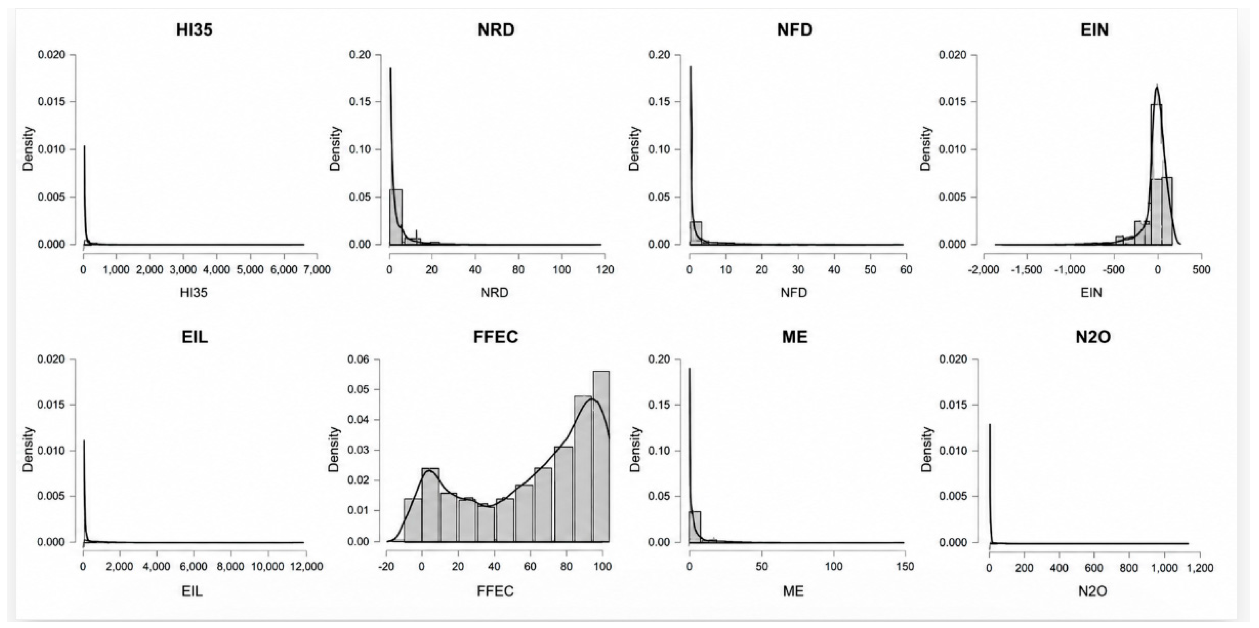
Figure A2.
Boxplots and Violin Plots of Key Environmental and Energy Variables Related to Heat Exposure and Sustainability.
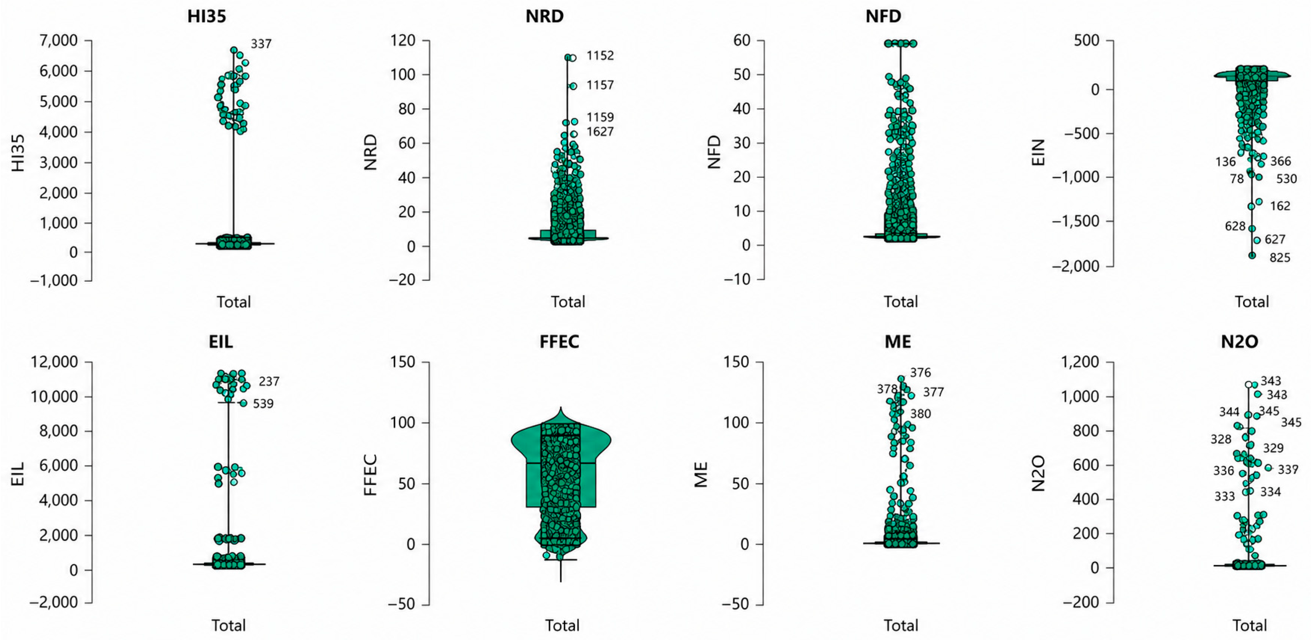
Figure A3.
Q-Q Plots for Distributional Assessment of Environmental and Climate Variables.
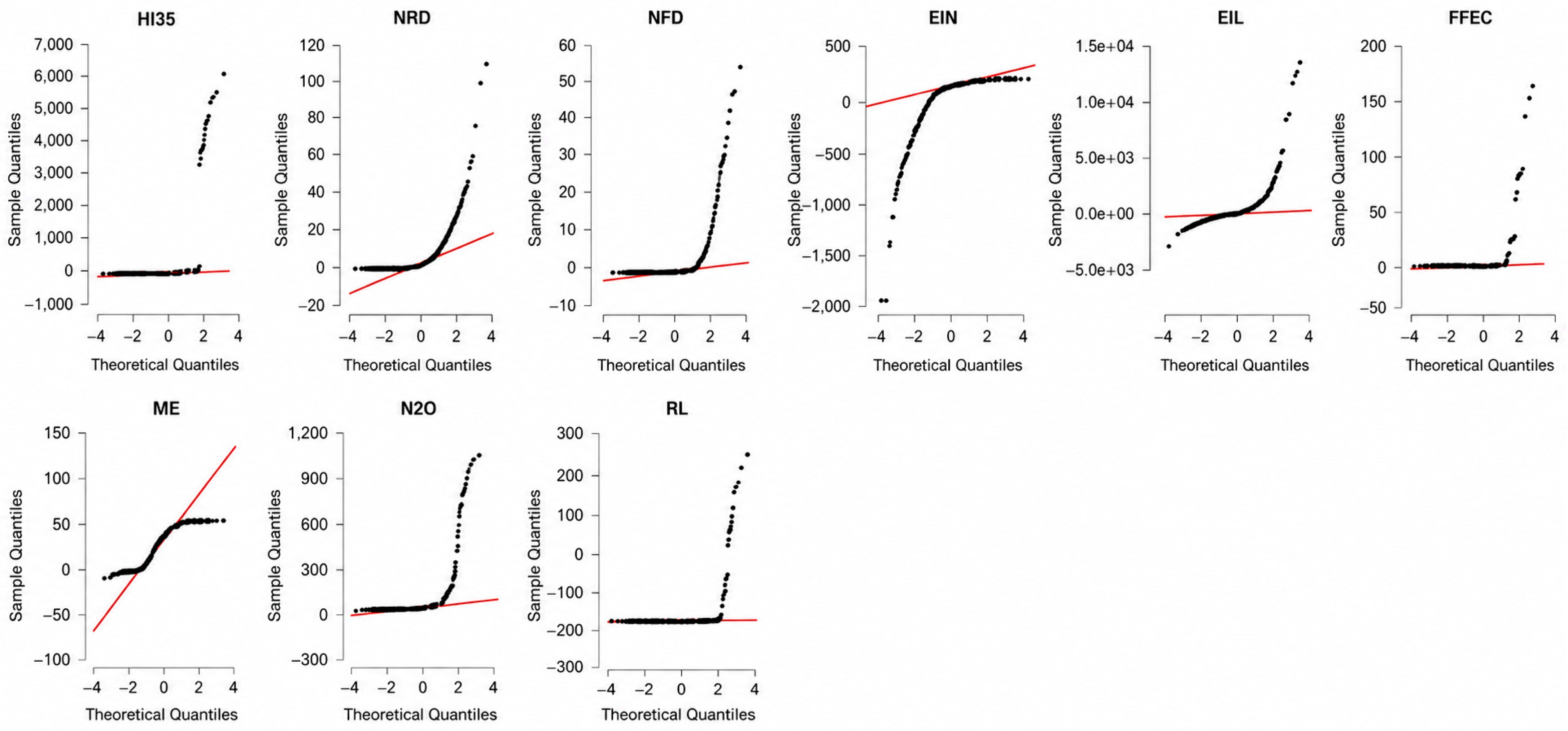
Figure A4.
HI35 and ESG Dimension Interactions: Scatter and Density Plots.
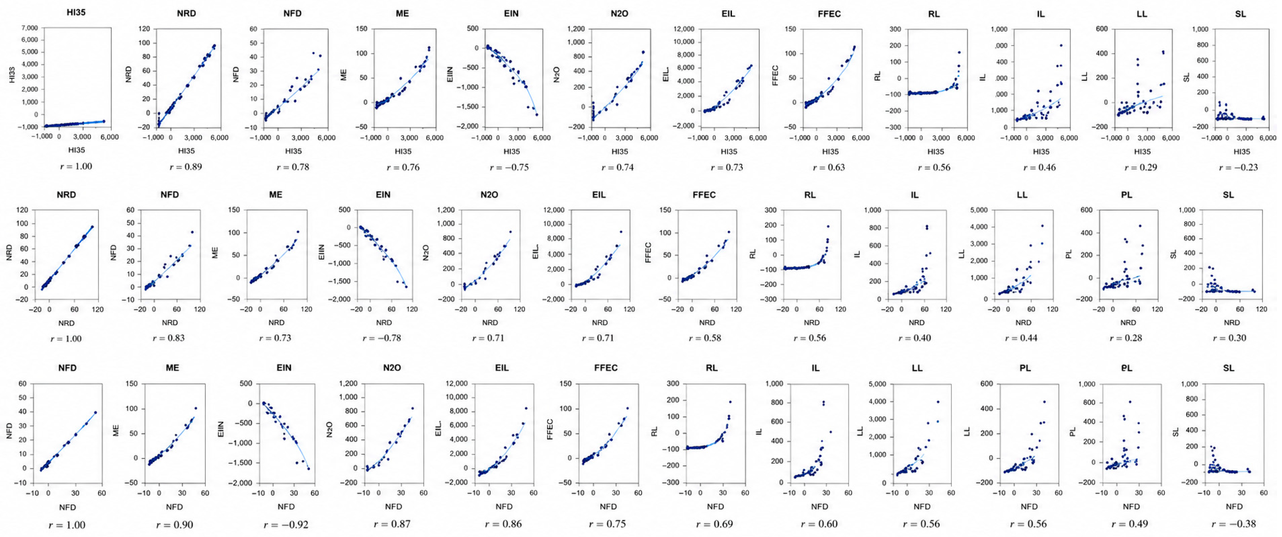
Appendix B. Descriptive and Statistical Diagnostics of HI35 and Social Sustainability Indicators
Table A2.
Descriptive Statistics of HI35 and Social Sustainability Indicators: Fertility, Water Access, and Undernourishment.
Figure A5.
Distribution Plots of HI35 and Social ESG Indicators (FR, PUSM, and POU).
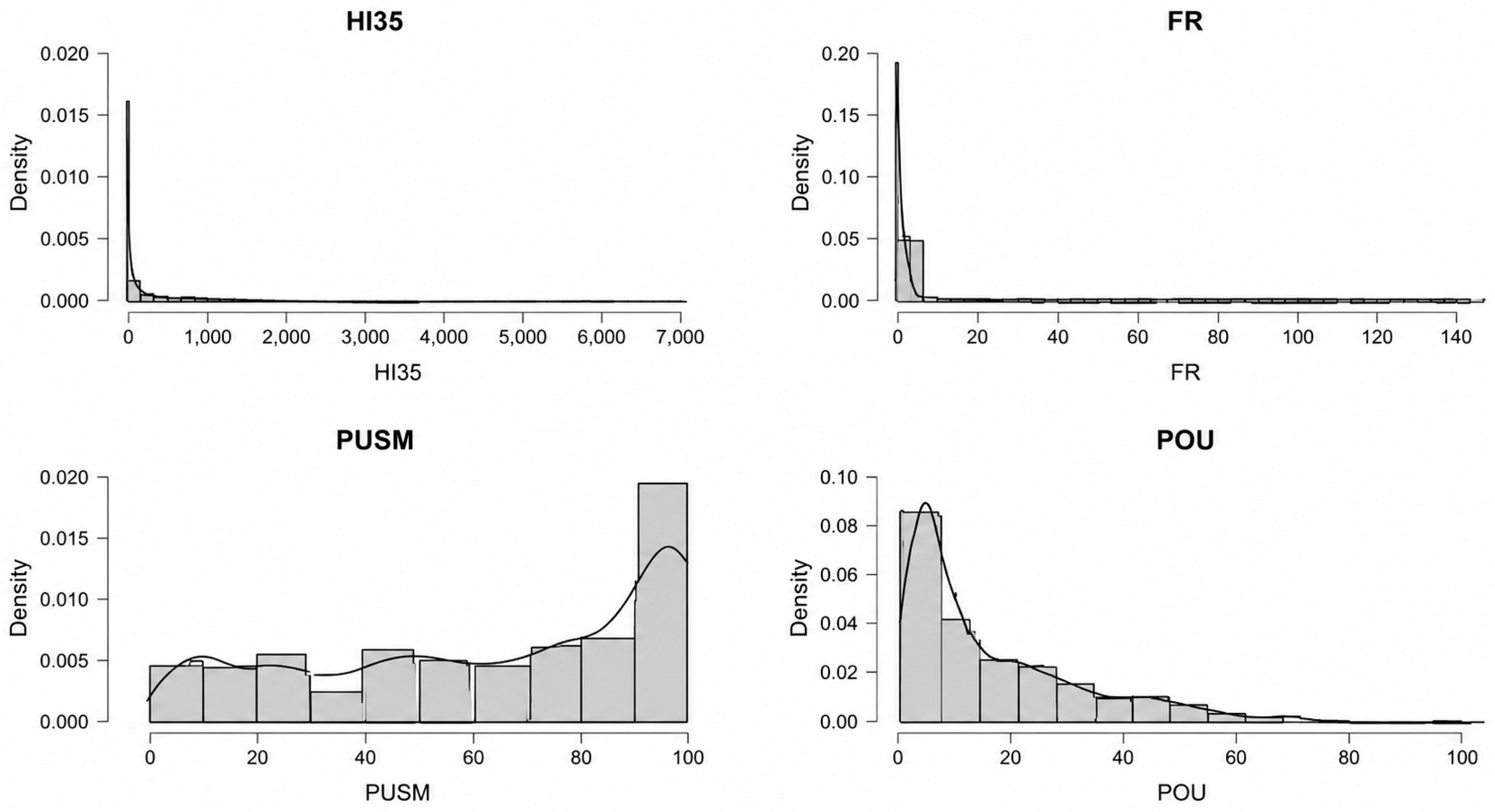
Figure A6.
Scatterplot Matrix of HI35 and Social ESG Indicators (FR, PUSM, and POU).
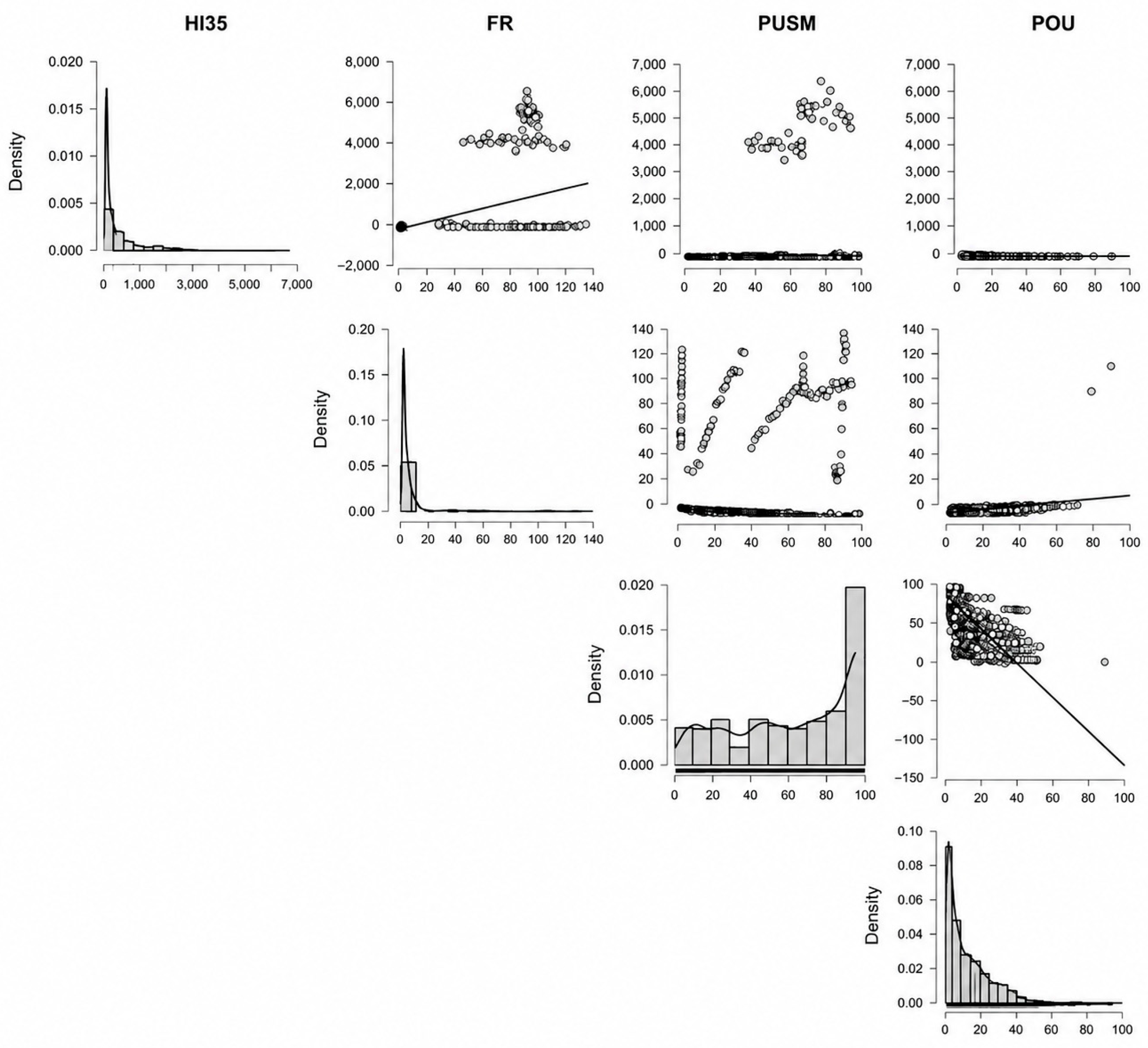
Figure A7.
Q–Q Plots of HI35 and Social ESG Indicators (FR, PUSM, and POU).
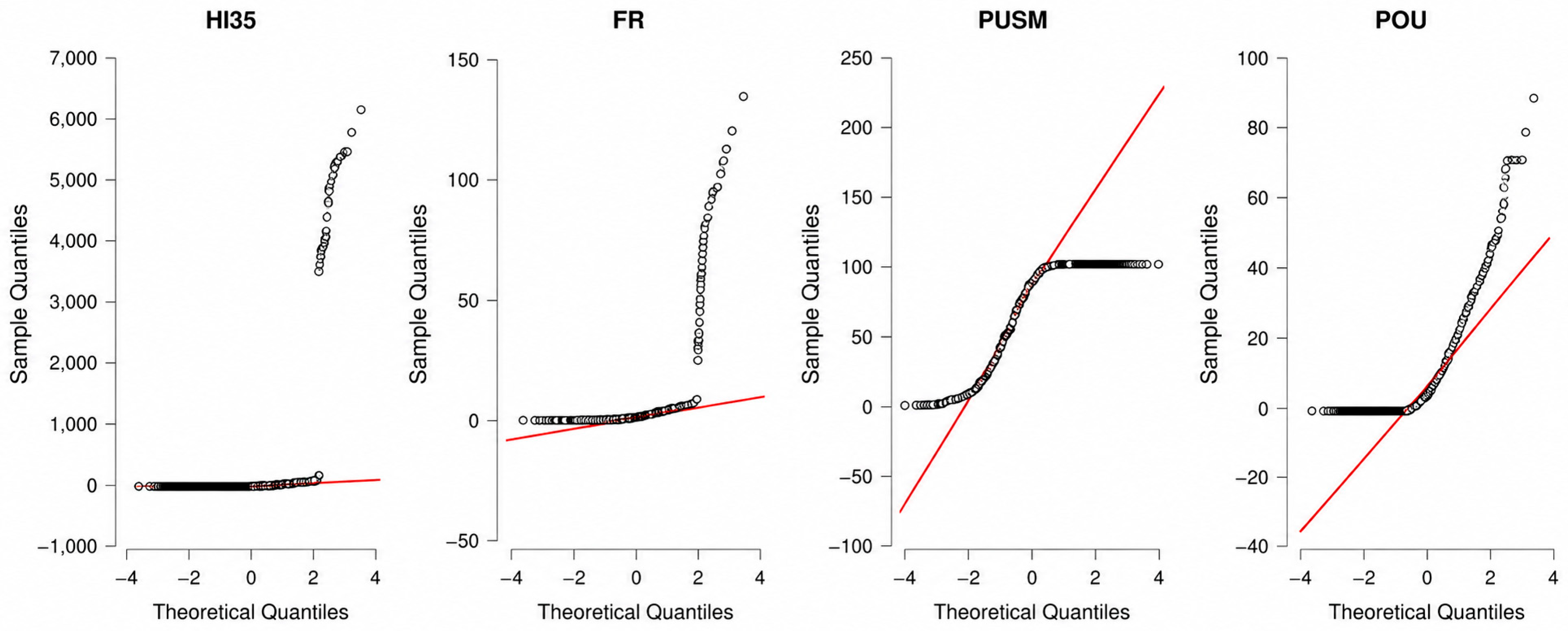
Appendix C. Descriptive Analysis of Governance Structures and Climate Stress Exposure Across Nations
Table A3.
Descriptive Statistics of HI35 and Leading Governance Indicators: Economic Growth, Political Stability, Gender Equality, Legal Strength, and Innovation Capacity.
Figure A8.
Distribution Plots of HI35 and Governance Indicators: Institutional Quality and Climate Stress Across Countries.
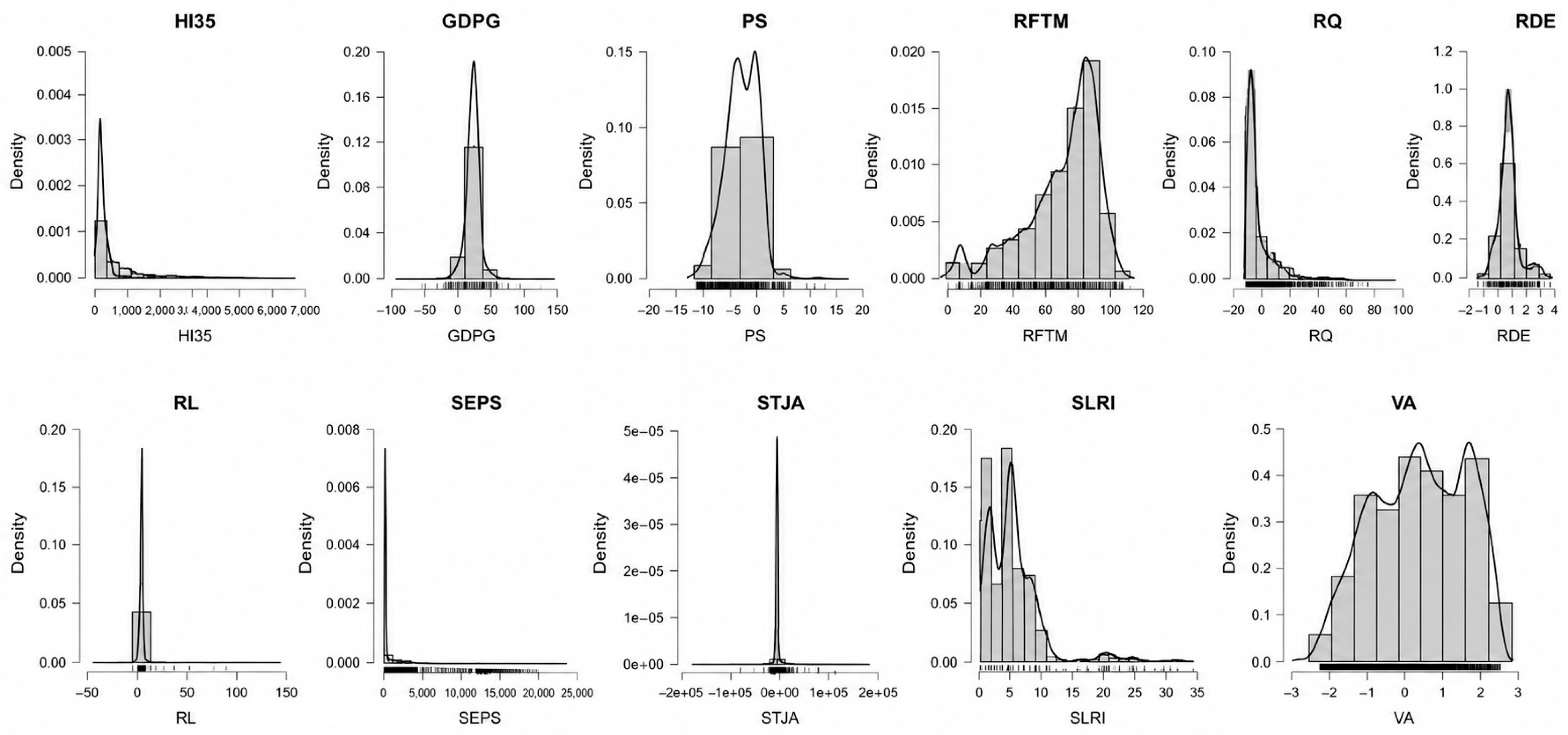
Figure A9.
Correlation Scatterplot Matrix of HI35 and Governance Indicators.
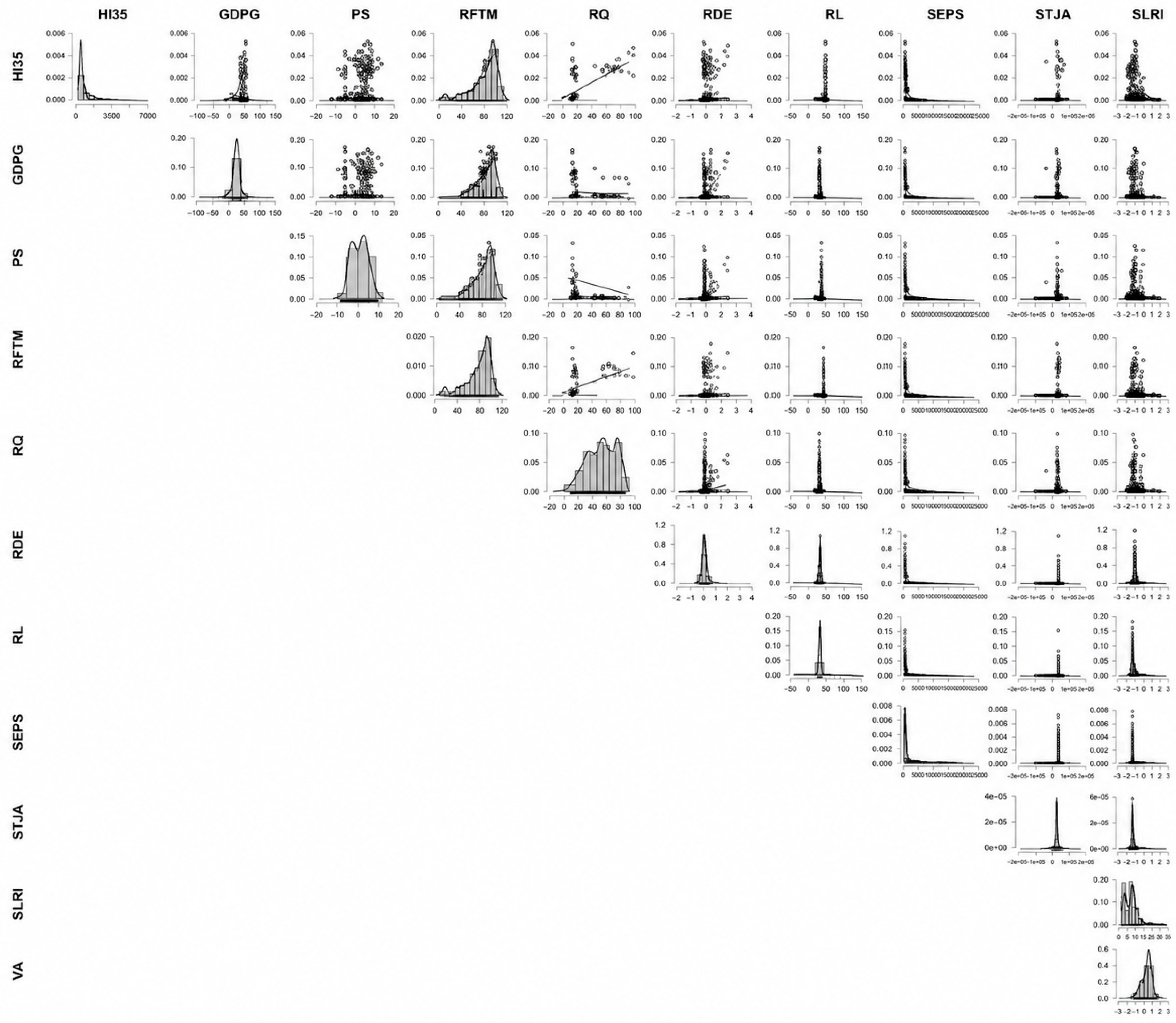
Figure A10.
Boxplot Distribution of Climate Stress and Governance Indicators.
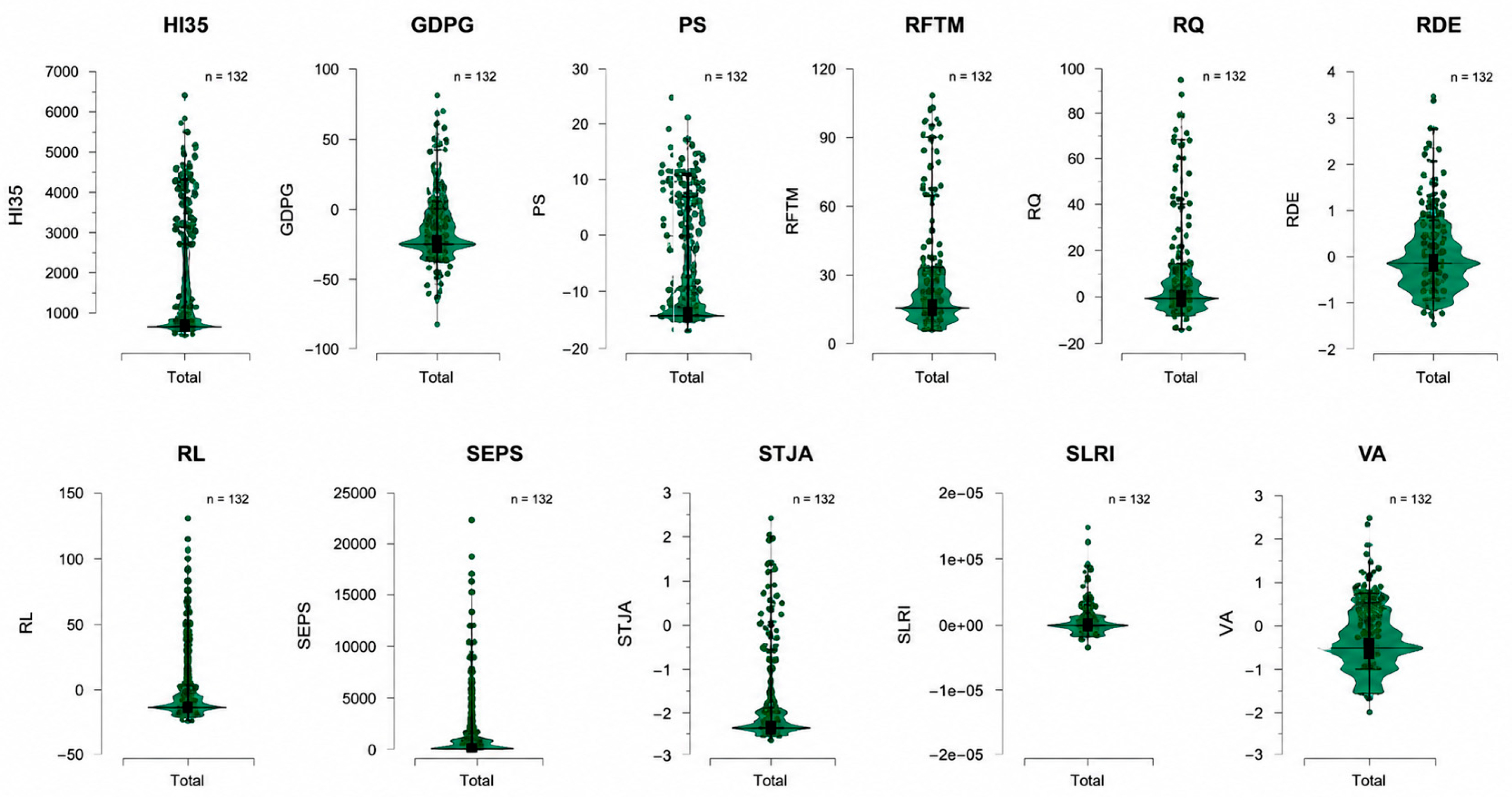
Figure A11.
Q-Q Plots Assessing Normality of Climate Stress and Governance Indicators.
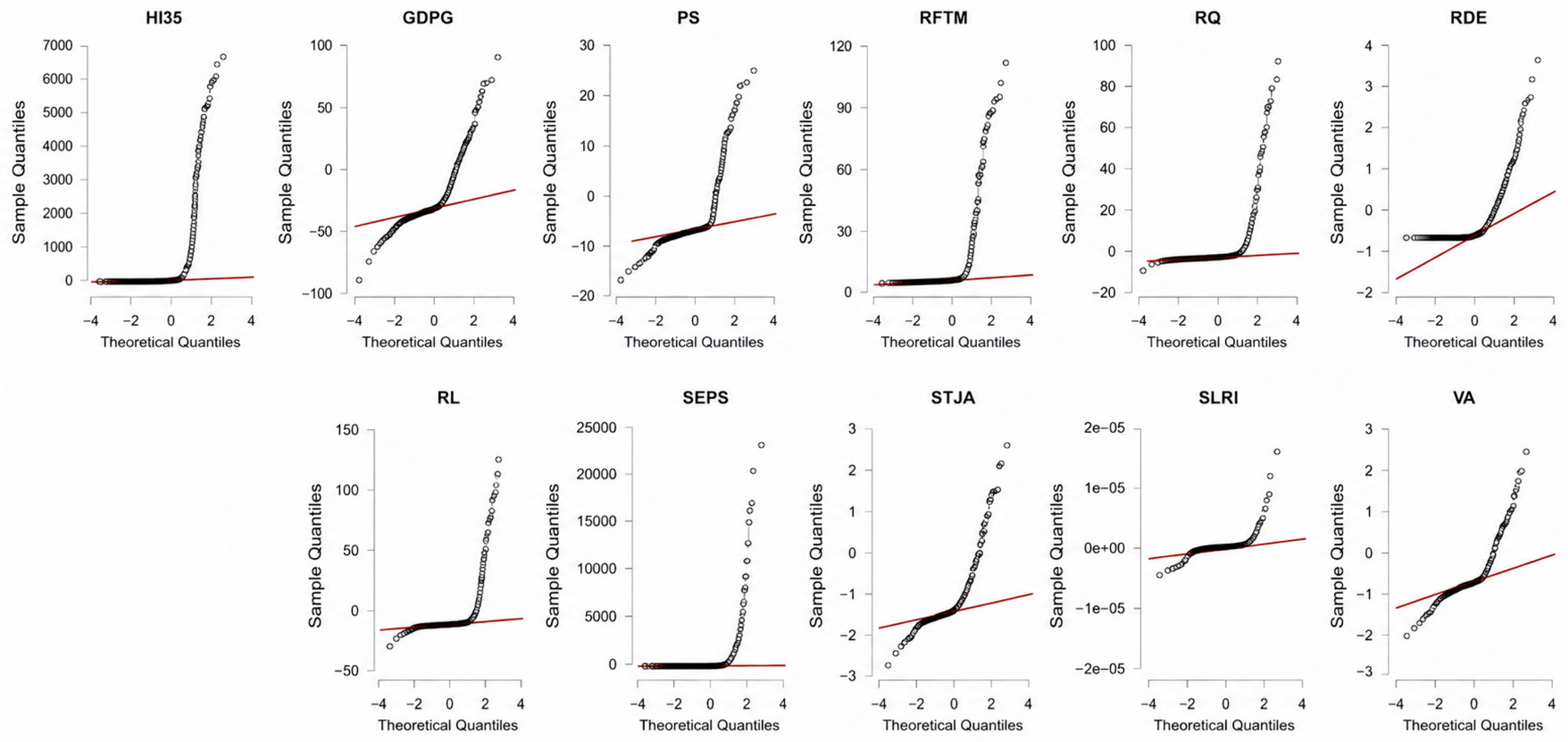
Figure A12.
Governance and Climate Stress—Scatter Matrix of Institutional Interactions.
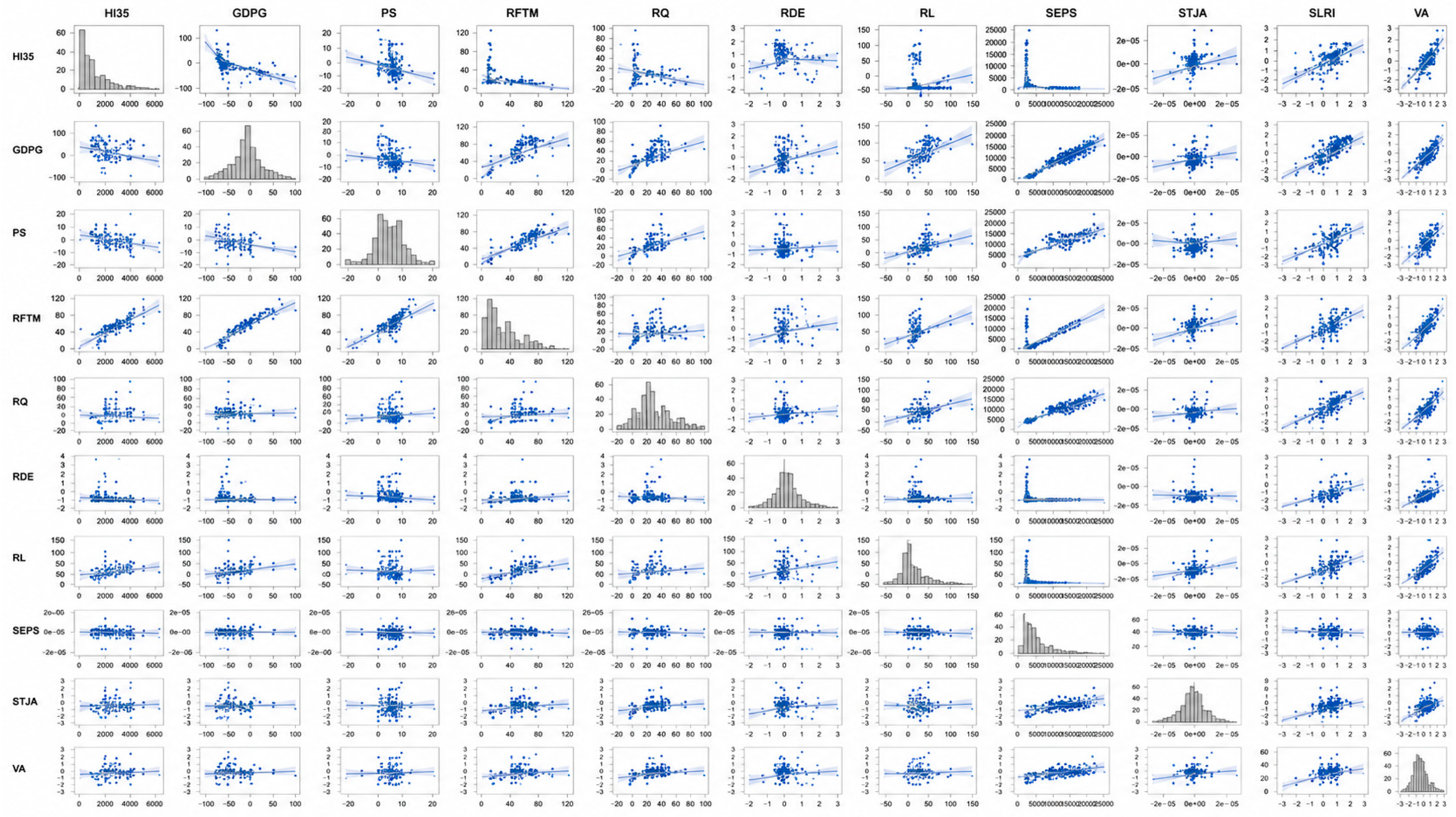
Table A4.
Covariance Matrix of Climate Stress (HI35) and Governance Indicators: Institutional Quality, Scientific Capacity, and Legal Structures.
Table A5.
Correlation Matrix between Climate Stress (HI35) and Governance Indicators.
Appendix D. Long-Term Trends in National Heat Exposure (HI35), 2000–2022
Appendix D provides descriptive temporal evidence on the evolution of national HI35 values between 2000 and 2022. These time series are reported to contextualize the long-run HI35 averages used in the main clustering analysis. They are not used as direct inputs in the clustering algorithms, which rely on temporally averaged country-level indicators, nor are they used for temporal inference, trend estimation, or causal analysis. Their purpose is to show the historical variability and persistence of heat exposure across countries and to support the interpretation of HI35 as a long-run climatic exposure indicator.
Table A6.
Country-Level Heat Exposure (HI35) Across 78 Countries, 2000–2022.
References
- Alam, A.; Banna, H.; Alam, A.; Bhuiyan, M.; Mokhtar, N. Climate change and geopolitical conflicts: The role of ESG readiness. J. Environ. Manag. 2024, 353, 120284. [Google Scholar] [CrossRef] [Scilit]
- Yu, B.; Huang, G.; Zhou, X.; Wang, S.; Li, Y.; Wu, Y.; Ren, J. A stepwise-clustered heat stress downscaling approach to analyze future variations of heat stress in East China. Theor. Appl. Climatol. 2025, 156, 112. [Google Scholar] [CrossRef] [Scilit]
- Liu, H.; Zhang, Q.; Xia, X.; Yang, X.; Yi, Z.; Yue, L.; Huang, L. ESG performance and organizational resilience—Based on an “extreme heat event. Borsa Istanb. Rev. 2024, 24, 304–313. [Google Scholar]
- Liang, Y.; Tan, Q.; Pang, J. Bless or curse, how does extreme temperature shape heavy pollution companies’ ESG performance? Evidence from China. Energy Econ. 2024, 131, 107378. [Google Scholar] [CrossRef] [Scilit]
- Orlandi, L. Environmental Policies and Firms’ Financial Performance and Risks: Is the Environmental Score of European Firms a Tool for Financial Risk Mitigation and Financial Performance Improvement After the Heatwaves of August 2022? Masters’s Thesis, HEC-Ecole de Gestion de l’Université de Liège, Liège, Belgium, 2023. [Google Scholar]
- Li, C.; Tang, W.; Liang, F.; Wang, Z. The impact of climate change on corporate ESG performance: The role of resource misallocation in enterprises. J. Clean. Prod. 2024, 445, 141263. [Google Scholar] [CrossRef] [Scilit]
- Rossi, C.; Byrne, J.; Christiaen, C. Breaking the ESG rating divergence: An open geospatial framework for environmental scores. J. Environ. Manag. 2024, 349, 119477. [Google Scholar]
- Murari, K. Heat Resilience as a Key Element of City-Level Climate Action Plans. Confronting the Climate Crisis: Pathways to Urban Resilience in India; Observer Research Foundation: Delhi, India, 2023; Volume 4, p. 34. [Google Scholar]
- Jiang, Y.; Tang, Q. Mandatory carbon reporting, voluntary carbon disclosure and ESG performance. Pac. Account. Rev. 2023, 35, 534–561. [Google Scholar] [CrossRef] [Scilit]
- Marotta, A.; Porras-Amores, C.; Rodríguez Sánchez, A. Are green buildings an indicator of sustainable development? Appl. Sci. 2023, 13, 3005. [Google Scholar] [CrossRef] [Scilit]
- Barotov, T. Climate Change Risk Premium, Stock Returns and Volatility Analysis in Relation to ESG Score. Master’s Thesis, Faculty of Social Sciences, Institute of Economic Studies, Charles University, Prague, Czech Republic, 2022. [Google Scholar]
- Iqbal, N.; Bouri, E.; Shahzad, S.; Alsagr, N. Asymmetric impacts of Chinese climate policy uncertainty on Chinese asset prices. Energy Econ. 2024, 133, 107518. [Google Scholar] [CrossRef] [Scilit]
- Capriotti, A.; Muzzioli, S. Climate Risk Measures and Main Data Providers; DEMB Working Paper Series; Dipartimento di Economia Marco Biagi: Modena, Italy, 2024. [Google Scholar]
- Zhu, Y.; Carrasco, L. Where is biodiversity in ESG? Environmental, social and governance (ESG) assessments largely overlook biodiversity. Resour. Conserv. Recycl. 2025, 217, 108187. [Google Scholar] [CrossRef] [Scilit]
- Lupu, I.; Hurduzeu, G.; Lupu, R. How is the ESG reflected in European financial stability? Sustainability 2022, 14, 10287. [Google Scholar] [CrossRef] [Scilit]
- Feng, X.; von Mettenheim, H.; Sermpinis, G.; Stasinakis, C. Sustainable Portfolio Construction via Machine Learning: ESG, SDG and Sentiment. In European Financial Management; John Wiley & Sons Ltd.: Hoboken, NJ, USA, 2024. [Google Scholar]
- Bebchuk, L.; Tallarita, R. The perils and questionable promise of ESG-based compensation. J. Corp. Law. 2022, 48, 37–75. [Google Scholar]
- Pompella, M.; Costantino, L. ESG disclosure and sustainability transition: A new metric and emerging trends in responsible investments. TalTech J. Eur. Stud. 2023, 13, 8–39. [Google Scholar] [CrossRef] [Scilit]
- Jiang, P.; Feng, G.; Wang, H.; Chang, C. CSR from different perspectives: The global ESG indexes updated. Corp. Soc. Responsib. Environ. Manag. 2024, 31, 4694–4714. [Google Scholar] [CrossRef] [Scilit]
- Wang, L.; Ji, Y.; Ni, Z. Spillover of stock price crash risk: Do environmental, social and governance (ESG) matter? Int. Rev. Financ. Anal. 2023, 89, 102768. [Google Scholar] [CrossRef] [Scilit]
- Luo, L.; Tang, Q. The real effects of ESG reporting and GRI standards on carbon mitigation: International evidence. Bus. Strategy Environ. 2023, 32, 2985–3000. [Google Scholar]
- Oliver Yébenes, M. Climate change, ESG criteria and recent regulation: Challenges and opportunities. Eurasian Econ. Rev. 2024, 14, 87–120. [Google Scholar] [CrossRef] [Scilit]
- Jinga, P. Governance (ESG) Investing in Combating Climate Change. In Environmental Management: Pollution, Habitat, Ecology, and Sustainability; Intechopen: London, UK, 2022; Volume 279. [Google Scholar]
- Oza, P.; Singhal, P. A Study of Factors Influencing Environmental, Social and Governance (ESG) Investing Among Retail Investors in India; Faculty of Management Studies and Commerce University of Sri Jayewardenepura: Nugegoda, Sri Lanka, 2024. [Google Scholar]
- Yu, L.; Keilani, A.; Tran, N.N.; Escribà-Gelonch, M.; Goodsite, M.; Sandhu, S.; Hessel, V. ESG assessment methodology for emerging technologies: Plasma versus conventional technology for ammonia production. Rsc Sustain. 2025, 3, 1102–1113. [Google Scholar] [PubMed]
- Xu, X.; Zhao, H. An Empirical Study on ESG Evaluation of Chinese Energy Enterprises Based on High-Quality Development Goals—A Case Study of Listed Company Data. Sustainability 2024, 16, 6602. [Google Scholar] [CrossRef] [Scilit]
- Ren, M.; Zhou, J.; Si, J.; Wang, G.; Guo, C. The impact of ESG performance on green innovation among traditional energy en-terprises—Evidence from listed companies in China. Sustainability 2024, 16, 3542. [Google Scholar] [CrossRef] [Scilit]
- Treepongkaruna, S.; Au Yong, H.; Thomsen, S.; Kyaw, K. Greenwashing, carbon emission, and ESG. Bus. Strategy Env. 2024, 33, 8526–8539. [Google Scholar] [CrossRef] [Scilit]
- Rasool, N.; Arunachalam, M.; Wellalage, N.; Kumar, V. Unveiling the relationship between ESG and growth of unlisted firms: Empirical insights from Eastern Europe and Central Asia. Bus. Strategy Environ. 2025, 34, 5669–5686. [Google Scholar] [CrossRef] [Scilit]
- Trinh, H.H. Corporate ESG Profile, Innovation Investment, and Cost of Debt Financing: Global Evidence from Uncertainty Episodes. Strateg. Bus. Res. 2026, 2, 100079. [Google Scholar] [CrossRef] [Scilit]
- Trinh, H.H. Global Economic Policy Uncertainty, Corporate ESG Ratings, and Default Probability Risk in the Era of Climate Change. SSRN. Available online: https://ssrn.com/abstract=4697422 (accessed on 17 January 2024).
- De Giovanni, P. Why Nobody Measures the Scope 4 (Avoided) Emissions? Let’s Get It Started! Sustainability 2025, 17, 8317. [Google Scholar] [CrossRef] [Scilit]
- Hu, C.; Guo, R. Research on risk contagion in ESG industries: An information entropy-based network approach. Entropy 2024, 26, 206. [Google Scholar] [CrossRef] [Scilit] [PubMed]
- Verma, R.; Mohnot, R. Relative impact of the US energy market sentiments on stocks and ESG index returns: Evidence from GCC countries. Int. J. Energy Econ. Policy 2023, 13, 290–300. [Google Scholar] [CrossRef] [Scilit]
- Yu, Y.; Meng, X.; Ren, C. The Impact of Extreme Temperature on Enterprise ESG: An Empirical Analysis of China. Green. Low.-Carbon Econ. 2026, 4, 9–20. [Google Scholar]
- Liu, K.; Fu, Z.; Chai, Y. Efficiency Calculation and Analysis of Green Economy Based on Improved Fixed Effects Model. IEEE Access 2024, 12, 162714–162728. [Google Scholar] [CrossRef] [Scilit]
- Sugiarto, A.; Puspani, N.; Fathia, F. ESG leverage towards stock performance in Indonesia stock exchange. Int. J. Energy Econ. Policy 2023, 13, 593–606. [Google Scholar] [CrossRef] [Scilit]
- Muddasir, M.; Ramon-Llorens, M. Impact of Macroeconomic Factors on S&P Europe 350 ESG Index During the Rus-so-Ukrainian War. Sci. Ann. Econ. Bus. 2025, 72, 145–164. [Google Scholar]
- Tan, J.; Zou, X.; Zhang, X.; Chang, C. Does national ESG performance move together with climate warming? Econ. Anal. Policy 2025, 86, 19–29. [Google Scholar] [CrossRef] [Scilit]
- Lee, E.; Kim, G. Analysis of domestic and international green infrastructure research trends from the ESG perspective in South Korea. Int. J. Environ. Res. Public Health 2022, 19, 7099. [Google Scholar] [CrossRef] [Scilit] [PubMed]
- Semet, R.; Roncalli, T.; Stagnol, L. ESG and sovereign risk: What is priced in by the bond market and credit rating agencies? 2021. Available online: https://ssrn.com/abstract=3940945 (accessed on 28 December 2025).
- He, J.; Wu, F. Sovereigns and ESG: Taking a Stance in a Complicated World; JP Morgan Asset Management: Mumbai, India, 2022. [Google Scholar]
- Enriquez, R.; Hillbom, E.; Palacio, A. Can Sovereign ESG Help Guide Nation-States’ Transformative Change? J. Sustain. Dev. 2025, 18, 56–76. [Google Scholar]
- Chen, X.; Huang, R.; Zhang, X.; Zhang, Y.; Yu, Y.; Otaki, T.; Shaw, R. Synergies and Gaps in ESG, Climate Disasters, and Social Inequality: A Literature Review. Climate 2025, 13, 241. [Google Scholar] [CrossRef] [Scilit]
- Manjengwa, E.; Dunga, S.; Mncayi-Makhanya, P.; Makhalima, J. ESG performance and economic growth in BRICS countries: A dynamic ARDL panel approach. Sustainability 2025, 17, 6334. [Google Scholar] [CrossRef] [Scilit]
- Mouti, K.; Kilincarslan, E.; Li, J. Environmental credit risk, climate change and bank performance: Evidence from a global panel of banks. Bus. Strategy Environ. 2026, 35, 1646–1666. [Google Scholar]
- Wang, H.; Zhou, L.; Xu, J.; Shan, J. Can National ESG Inhibit the Impact of Extreme Climate on Global Financial Risks? In International Studies of Economics; John Wiley & Sons: Hoboken, NJ, USA, 2025. [Google Scholar]
- Lanzante, J. A new heat stress index for climate change assessment. Bull. Am. Meteorol. Soc. 2024, 105, E2482–E2495. [Google Scholar] [CrossRef] [Scilit]
- Alvarez, I.; Diaz-Poso, A.; Lorenzo, M.; Roye, D. Heat index historical trends and projections due to climate change in the Mediterranean basin based on CMIP6. Atmos. Res. 2024, 308, 107512. [Google Scholar] [CrossRef] [Scilit]
- Zitouni, D.; Berkouk, D.; Matallah, M.; Ben Ratmia, M.; Attia, S. Advancing Heat Health Risk Assessment: Hotspot Identification of Heat Stress and Risk Across Municipalities in Algiers, Algeria. Atmosphere 2025, 16, 484. [Google Scholar] [CrossRef] [Scilit]
- Chander, S.; Vijaya, P. Unsupervised learning methods for data clustering. Artif. Intell. Data Min. 2021, 3, 41–64. [Google Scholar] [CrossRef] [Scilit]
- Mishra, B.; Pandey, O.; Dehuri, S.; Cho, S. Unsupervised functional link artificial neural networks for cluster analysis. IEEE Access 2020, 8, 169215–169228. [Google Scholar] [CrossRef] [Scilit]
- Sinaga, K.; Yang, M. Unsupervised K-means clustering algorithm. IEEE Access 2020, 8, 80716–80727. [Google Scholar] [CrossRef] [Scilit]
- Saxena, A.; Prasad, M.; Gupta, A.; Bharill, N.; Patel, O.; Tiwari, A.; Er, M.; Ding, W.; Lin, C.-T. A review of clustering tech-niques and developments. Neurocomputing 2017, 267, 664–681. [Google Scholar]
- Hancer, E.; Xue, B.; Zhang, M. A survey on feature selection approaches for clustering. Artif. Intell. Rev. 2020, 53, 4519–4545. [Google Scholar] [CrossRef] [Scilit]
- Hennig, C. Cluster-wise assessment of cluster stability. Comput. Stat. Data Anal. 2007, 52, 258–271. [Google Scholar] [CrossRef] [Scilit]
- De Amorim, R.; Hennig, C. Recovering the number of clusters in data sets with noise features using feature rescaling factors. Inf. Sci. 2015, 324, 126–145. [Google Scholar] [CrossRef] [Scilit]
- Charrad, M.; Ghazzali, N.; Boiteau, V.; Niknafs, A. NbClust: An R package for determining the relevant number of clusters in a data set. J. Stat. Softw. 2014, 61, 1–36. [Google Scholar] [CrossRef] [Scilit]
- Wattanatorn, W. Climate change exposure, circular economy and default probability: Global evidence. Cogent Econ. Financ. 2025, 13, 2544175. [Google Scholar] [CrossRef] [Scilit]
- Jiang, W.; Hu, Y.; Nistor, S.; Xu, Y. Bank profitability under environmental and climate pressures: The case of European banks. J. Appl. Econ. 2025, 28, 2491397. [Google Scholar] [CrossRef] [Scilit]
- Karkowska, R.; Samaniego-Medina, R.; Giráldez-Puig, P.; Korzeb, Z. Boards and ESG performance: The contingent influence of climate vulnerability on global banks. Bus. Strategy Environ. 2026, 35, 2842–2863. [Google Scholar]
- Katta, V.; Shrivastava, G.; Kushwah, V. Hierarchical K-means clustering of earthquake data for in-depth spatial and magnitude analysis in Gujarat India. Multidiscip. Sci. J. 2024, 7, 2025325. [Google Scholar]
- Sterzel, T.; Lüdeke, M.; Walther, C.; Kok, M.; Sietz, D.; Lucas, P. Typology of coastal urban vulnerability under rapid urbanization. PLoS ONE 2020, 15, e0220936. [Google Scholar] [CrossRef] [Scilit] [PubMed]
- D’Orazio, P. Mapping the emergence and diffusion of climate-related financial policies: Evidence from a cluster analysis on G20 countries. Int. Econ. 2022, 169, 135–147. [Google Scholar] [CrossRef] [Scilit]
- Kocur-Bera, K.; Czyża, S. Socio-economic vulnerability to climate change in rural areas in the context of green energy devel-opment—A study of the great Masurian Lakes Mesoregion. Int. J. Environ. Res. Public Health 2023, 20, 2689. [Google Scholar] [PubMed]
- Pathiranage, H. Navigating the trade-offs between economic growth and environmental sustainability: A global analysis of long-term trends and strategic policies. Sustain. Environ. 2024, 10, 2419161. [Google Scholar] [CrossRef] [Scilit]
- Matviychuk, A.; Zhytkevych, O.; Osadcha, N. Modeling carbon dioxide emissions reduction. Energy Rep. 2024, 12, 1876–1887. [Google Scholar] [CrossRef] [Scilit]
- Baloch, M.; Khan, S.; Ulucak, Z.; Ahmad, A. Analyzing the relationship between poverty, income inequality, and CO2 emission in Sub-Saharan African countries. Sci. Total Environ. 2020, 740, 139867. [Google Scholar] [CrossRef] [Scilit] [PubMed]
- Khan, I.; Hou, F.; Le, H.; Ali, S. Do natural resources, urbanization, and value-adding manufacturing affect environmental quality? Evidence from the top ten manufacturing countries. Resour. Policy 2021, 72, 102109. [Google Scholar] [CrossRef] [Scilit]
- Acheampong, A.; Boateng, E.; Amponsah, M.; Dzator, J. Revisiting the economic growth–energy consumption nexus: Does globalization matter? Energy Econ. 2021, 102, 105472. [Google Scholar] [CrossRef] [Scilit]
- Shahzad, U.; Radulescu, M.; Rahim, S.; Isik, C.; Yousaf, Z.; Ionescu, S. Do environment-related policy instruments and tech-nologies facilitate renewable energy generation? Exploring the contextual evidence from developed economies. Energies 2021, 14, 690. [Google Scholar]
- Zhao, X.; Mahendru, M.; Ma, X.; Rao, A.; Shang, Y. Impacts of environmental regulations on green economic growth in China: New guidelines regarding renewable energy and energy efficiency. Renew. Energy 2022, 187, 728–742. [Google Scholar]
- Sharif, A.; Aloui, C.; Yarovaya, L. COVID-19 pandemic, oil prices, stock market, geopolitical risk and policy uncertainty nexus in the US economy: Fresh evidence from the wavelet-based approach. Int. Rev. Financ. Anal. 2020, 70, 101496. [Google Scholar] [CrossRef] [Scilit] [PubMed]
- Romanello, M.; di Napoli, C.; Green, C.; Kennard, H.; Lampard, P.; Scamman, D.; Walawender, M.; Ali, Z.; Ameli, N.; Ayeb-Karlsson, S.; et al. The 2023 report of the Lancet Countdown on health and climate change: The imperative for a health-centred response in a world facing irreversible harms. The Lancet 2023, 402, 2346–2394. [Google Scholar] [CrossRef] [Scilit]
- Béné, C.; Fanzo, J.; Prager, S.; Achicanoy, H.; Mapes, B.; Alvarez Toro, P.; Bonilla Cedrez, C. Global drivers of food system (un) sustainability: A multi-country correlation analysis. PLoS ONE 2020, 15, e0231071. [Google Scholar] [PubMed]
- Vicedo-Cabrera, A.; Scovronick, N.; Sera, F.; Royé, D.; Schneider, R.; Tobias, A.; Gasparrini, A. The burden of heat-related mortality attributable to recent human-induced climate change. Nat. Clim. Change 2021, 11, 492–500. [Google Scholar] [CrossRef] [Scilit]
- Hasegawa, T.; Fujimori, S.; Takahashi, K.; Yokohata, T.; Masui, T. Economic implications of climate change impacts on human health through undernourishment. Clim. Change 2016, 136, 189–202. [Google Scholar] [CrossRef] [Scilit]
- Murphy, D. Theorizing climate change, (im)mobility and socio-ecological systems resilience in low-elevation coastal zones. Clim. Dev. 2015, 7, 380–397. [Google Scholar]
- Fränti, P.; Sieranoja, S. How much can k-means be improved by using better initialization and repeats? Pattern Recognit. 2019, 93, 95–112. [Google Scholar] [CrossRef] [Scilit]
- Rodriguez, M.; Comin, C.; Casanova, D.; Bruno, O.; Amancio, D.; Costa, L.; Rodrigues, F. Clustering algo-rithms: A comparative approach. PLoS ONE 2019, 14, e0210236. [Google Scholar] [CrossRef] [Scilit] [PubMed]
- Xu, D.; Tian, Y. A comprehensive survey of clustering algorithms. Ann. Data Sci. 2015, 2, 165–193. [Google Scholar] [CrossRef] [Scilit]
- Bayliss, A. Validating Classical Multivariate Models in Archaeology: English Medieval Bellfounding as a Case Study. Doctoral Dissertation, University of London, London, UK, 2006. [Google Scholar]
- Jain, A. Data clustering: 50 years beyond K-means. Pattern Recognit. Lett. 2010, 31, 651–666. [Google Scholar] [CrossRef] [Scilit]
- Mukherjee, S.; Mishra, A.; Trenberth, K. Climate change and drought: A perspective on drought indices. Curr. Clim. Change Rep. 2018, 4, 145–163. [Google Scholar] [CrossRef] [Scilit]
- Wutich, A.; Ragsdale, K. Water insecurity and emotional distress: Coping with supply, access, and seasonal variability of water in a Bolivian squatter settlement. Soc. Sci. Med. 2008, 67, 2116–2125. [Google Scholar] [PubMed]
- Diffenbaugh, N.; Burke, M. Global warming has increased global economic inequality. Proc. Natl. Acad. Sci. USA 2019, 116, 9808–9813. [Google Scholar] [CrossRef] [Scilit] [PubMed]
- Stoler, J.; Brewis, A.; Kangmennang, J.; Keough, S.; Pearson, A.; Rosinger, A.; Stauber, C.; Stevenson, E. Connecting the dots between climate change, household water insecurity, and migration. Curr. Opin. Environ. Sustain. 2021, 51, 36–41. [Google Scholar] [CrossRef] [Scilit]
- Gagolewski, M.; Bartoszuk, M.; Cena, A. Are cluster validity measures (in) valid? Inf. Sci. 2021, 581, 620–636. [Google Scholar] [CrossRef] [Scilit]
- Da Silva, L.; Melton, N.; Wunsch, D. Incremental cluster validity indices for online learning of hard partitions: Exten-sions and comparative study. IEEE Access 2020, 8, 22025–22047. [Google Scholar]
- Blasilli, G.; Kerrigan, D.; Bertini, E.; Santucci, G. Towards a visual perception-based analysis of clustering quality metrics. In 2024 IEEE Visualization in Data Science (VDS); IEEE: St. Pete Beach, FL, USA, 2024; pp. 15–24. [Google Scholar]
- Sarmas, E.; Fragkiadaki, A.; Marinakis, V. Explainable AI-based ensemble clustering for load profiling and demand response. Energies 2024, 17, 5559. [Google Scholar] [CrossRef] [Scilit]
- La Marca, K.; Bedle, H.; Stright, L.; Marfurt, K. Uncertainty assessment in unsupervised machine-learning methods for deep-water channel seismic facies using outcrop-derived 3D models and synthetic seismic data. Interpretation 2024, 12, T303–T319. [Google Scholar]
- Duan, Y.; Lu, Z.; Wang, R.; Li, X.; Nie, F. Toward balance deep semisupervised clustering. In IEEE Transactions on Neural Net-works and Learning Systems; IEEE: Piscataway, NJ, USA, 2024. [Google Scholar]
- Vo Duy, A.; Che, Q.; Nguyen, V. Adaptive Scheme of Clustering-Based Unsupervised Learning for Person Re-identification. In Asian Conference on Intelligent Information and Database Systems; Springer: Singapore, 2024; pp. 193–205. [Google Scholar]
- Rosti, A.; Rota, M.; Penna, A. An empirical seismic vulnerability model. Bull. Earthq. Eng. 2022, 20, 4147–4173. [Google Scholar] [CrossRef] [Scilit]
- Kaufmann, D.; Kraay, A.; Mastruzzi, M. The worldwide governance indicators: Methodology and analytical issues. Hague J. Rule Law. 2011, 3, 220–246. [Google Scholar]
- Ouragini, I.; Ben Hassine Louzir, A. University social responsibility and sustainable development: Illustration of adapted prac-tices by two Tunisian Universities. Soc. Responsib. J. 2024, 20, 1177–1192. [Google Scholar]
- Mechkova, V.; Lührmann, A.; Lindberg, S. How much democratic backsliding? J. Democr. 2017, 28, 162–169. [Google Scholar]
- Joshi, D. Good governance, state capacity, and the millennium development goals. Perspect. Glob. Dev. Technol. 2011, 10, 339–360. [Google Scholar] [CrossRef] [Scilit]
- Hallegatte, S.; Rentschler, J.; Rozenberg, J. Adaptation Principles: A Guide for Designing Strategies for Climate Change Adaptation and Resilience; World Bank: Washington, DC, USA, 2020. [Google Scholar]
- Besley, T.; Persson, T. Democratic values and institutions. Am. Econ. Rev. Insights 2019, 1, 59–76. [Google Scholar] [CrossRef] [Scilit]
- Sachs, J.; Kroll, C.; Lafortune, G.; Fuller, G.; Woelm, F. Sustainable Development Report 2022; Cambridge University Press: Cambridge, UK, 2022. [Google Scholar]
- Dzigbede, K.; Gehl, S.; Willoughby, K. Disaster resiliency of US local governments: Insights to strengthen local response and recovery from the COVID-19 pandemic. Public Adm. Rev. 2020, 80, 634–643. [Google Scholar] [PubMed]
- Andrews, M.; Pritchett, L.; Woolcock, M. Building State Capability: Evidence, Analysis, Action; Oxford University Press: Oxford, UK, 2017. [Google Scholar]
- Li, P.; Chiou, J. Functional clustering and missing value imputation of traffic flow trajectories. Transp. B Transp. Dyn. 2021, 9, 1–21. [Google Scholar] [CrossRef] [Scilit]
- Călin, A.; Coroiu, A.; Mureşan, H. Analysis of preprocessing techniques for missing data in the prediction of sunflower yield in response to the effects of climate change. Appl. Sci. 2023, 13, 7415. [Google Scholar] [CrossRef] [Scilit]
- Si, Y.; Heeringa, S.; Johnson, D.; Little, R.; Liu, W.; Pfeffer, F.; Raghunathan, T. Multiple imputation with massive data: An ap-plication to the panel study of income dynamics. J. Surv. Stat. Methodol. 2023, 11, 260–283. [Google Scholar] [PubMed]
- Alejo-Sanchez, L.; Márquez-Grajales, A.; Salas-Martínez, F.; Franco-Arcega, A.; López-Morales, V.; Acevedo-Sandoval, O.; González-Ramírez, C.; Villegas-Vega, R. Missing data imputation of climate time series: A review. MethodsX 2025, 15, 103455. [Google Scholar] [CrossRef] [Scilit] [PubMed]
- Nugroho, H.; Surendro, K. A comprehensive bibliometric analysis of missing value imputation. IEEE Access 2024, 12, 14819–14846. [Google Scholar] [CrossRef] [Scilit]
- Dorabiala, O.; Aravkin, A.; Kutz, J. Ensemble principal component analysis. IEEE Access 2024, 1221, 6663–6671. [Google Scholar] [CrossRef] [Scilit]
- Mohammed, M.; Akawee, M.; Saleh, Z.; Hasan, R.; Ali, A.; Sutikno, T. The effectiveness of big data classification control based on principal component analysis. Bull. Electr. Eng. Inform. 2023, 12, 427–434. [Google Scholar] [CrossRef] [Scilit]
- Chen, F.; Rohe, K. A new basis for sparse principal component analysis. J. Comput. Graph. Stat. 2024, 33, 421–434. [Google Scholar]
- Barba, E.; Casamichana, D.; Figueiredo, P.; Nakamura, F.; Castellano, J. The Use of Principal Component Analysis for Reduction in Sleep Quality and Quantity Data in Female Professional Soccer. Sensors 2024, 25, 148. [Google Scholar] [PubMed]
- Eriksen, S.; Schipper, E.; Scoville-Simonds, M.; Vincent, K.; Adam, H.; Brooks, N.; Harding, B.; Khatri, D.; Lenaerts, L.; Liverman, D.; et al. Adaptation interventions and their effect on vulnerability in developing countries: Help, hindrance or irrelevance? World Dev. 2021, 141, 105383. [Google Scholar] [CrossRef] [Scilit]
- Thomas, K.; Hardy, R.; Lazrus, H.; Mendez, M.; Orlove, B.; Rivera-Collazo, I.; Roberts, J.; Rockman, M.; Warner, B.; Winthrop, R. Explaining differential vulnerability to climate change: A social science review. Wiley Interdiscip. Rev. Clim. Change 2019, 10, e565. [Google Scholar] [PubMed]
- Seneviratne, S.; Zhang, X.; Adnan, M.; Badi, W.; Dereczynski, C.; Luca, A.; Ghosh, S.; Iskandar, I.; Kossin, J.; Lewis, S.; et al. Weather and climate extreme events in a changing climate. In Climate Change 2021: The Physical Science Basis: Working Group I contribution to the Sixth Assessment Report of the Intergovernmental Panel on Climate Change; Cambridge University Press: Cambridge, UK, 2021; pp. 1513–1766. [Google Scholar]
- Carleton, T.; Jina, A.; Delgado, M.; Greenstone, M.; Houser, T.; Hsiang, S.; Hultgren, A.; E Kopp, R.; E McCusker, K.; Nath, I.; et al. Valuing the global mortality consequences of climate change accounting for adaptation costs and benefits. Q. J. Econ. 2022, 137, 2037–2105. [Google Scholar] [CrossRef] [Scilit]
- Cinner, J.; Adger, W.; Allison, E.; Barnes, M.; Brown, K.; Cohen, P.; Gelcich, S.; Hicks, C.; Hughes, T.; Lau, J.; et al. Building adaptive capacity to climate change in tropical coastal communities. Nat. Clim. Change 2018, 8, 117–123. [Google Scholar] [CrossRef] [Scilit]
- Newell, P.; Srivastava, S.; Naess, L.; Torres Contreras, G.; Price, R. Toward transformative climate justice: An emerging research agenda. Wiley Interdiscip. Rev. Clim. Change 2021, 12, e733. [Google Scholar] [CrossRef] [Scilit]
- Macnee, R.; Tokai, A. Heat wave vulnerability and exposure mapping for Osaka City, Japan. Environ. Syst. Decis. 2016, 36, 368–376. [Google Scholar] [CrossRef] [Scilit]
- Koman, P.; Romo, F.; Swinton, P.; Mentz, G.; de Majo, R.; Sampson, N.; Battaglia, M.; Hill-Knott, K.; Williams, G.; O’Neill, M.; et al. MI-Environment: Geospatial patterns and inequality of relative heat stress vulnerability in Michigan. Health Place 2019, 60, 102228. [Google Scholar] [CrossRef] [Scilit] [PubMed]
- Carrasco, C.; Hernandez-del-Valle, A. Energy intensity, economic structure, and capital goods imports in upper-middle income countries: Insights from HDBSCAN clustering. J. Environ. Manag. 2023, 339, 117840. [Google Scholar]
- Wijayanti, P.; Latifah, L.; Purwoko, S.; Riyanto, S.; Yunitawati, D.; Setyaji, T. Spatial Analysis of Drought Vulnerability Related to Climate Change and Under Five Children’s Nutritional Status. In BIO Web of Conferences; EDP Sciences: Les Ulis, France, 2024; Volume 133, p. 00019. [Google Scholar]
- Bista, R. Assessment of climate change induced household vulnerability in Nepal: Application of index method. ARRUS J. Soc. Sci. Humanit. 2023, 3, 9–20. [Google Scholar] [CrossRef] [Scilit]
- Albahouth, A.; Tahir, M. Institutional Quality and Climate Vulnerability: Empirical Evidence from GCC Economies. Sustainability 2025, 17, 2047. [Google Scholar] [CrossRef] [Scilit]
- Macharia, C.; Kiage, L. Conceptualizing heat vulnerability: Equity-centered approaches for comprehensive resilience in a changing climate. Nat. Hazards 2024, 120, 6923–6941. [Google Scholar] [CrossRef] [Scilit]
- Ofori, E.; Onifade, S.; Ali, E.; Alola, A.; Zhang, J. Achieving carbon neutrality in post COP26 in BRICS, MINT, and G7 economies: The role of financial development and governance indicators. J. Clean. Prod. 2023, 387, 135853. [Google Scholar] [CrossRef] [Scilit]
- Robertson, S.; Walker, G.; Horne, R. Tracing the ruptures and rhythms of summer heat, energy vulnerability and home. Geoforum 2024, 155, 104095. [Google Scholar] [CrossRef] [Scilit]
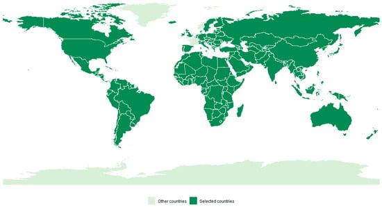
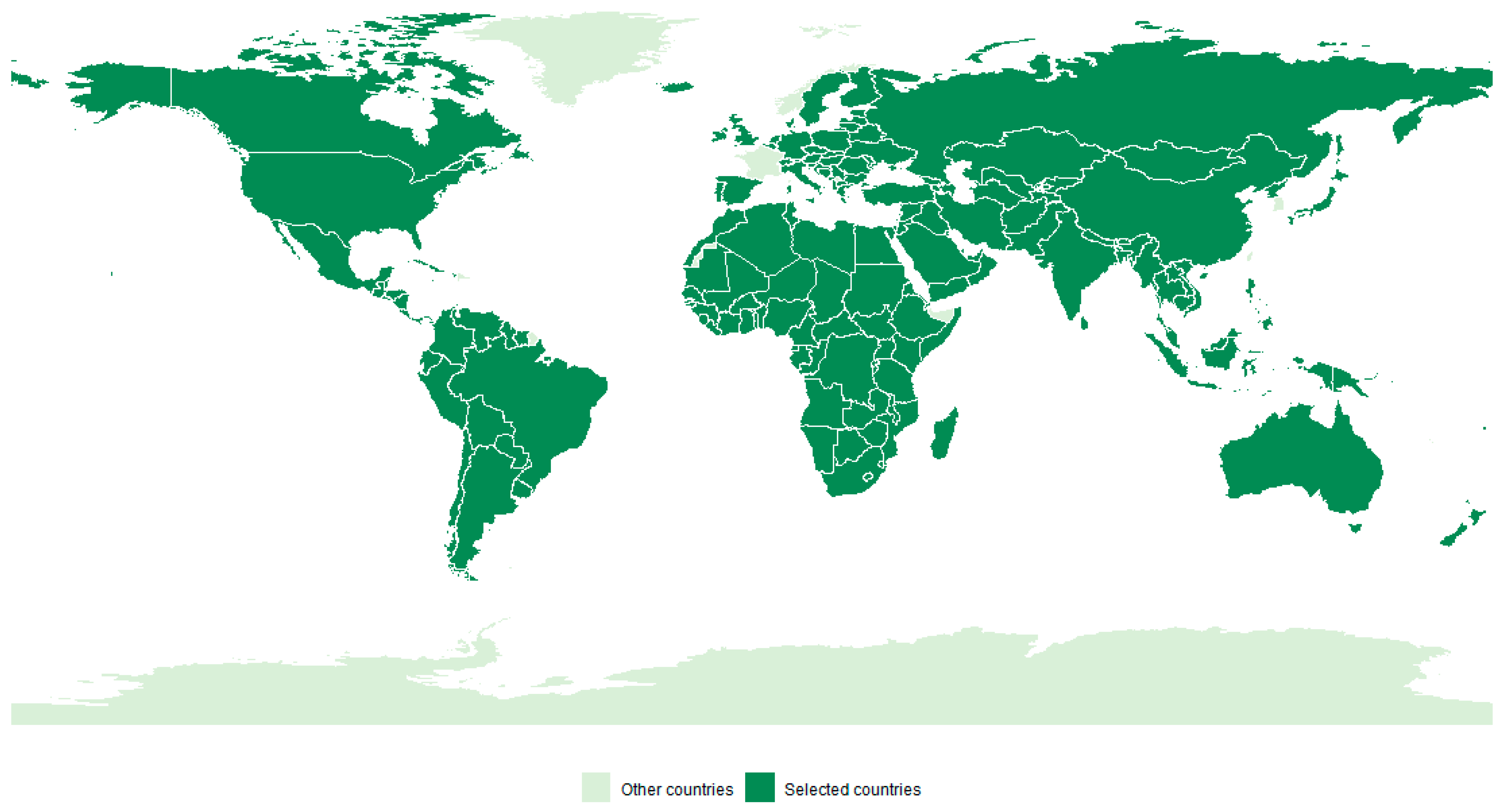
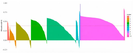
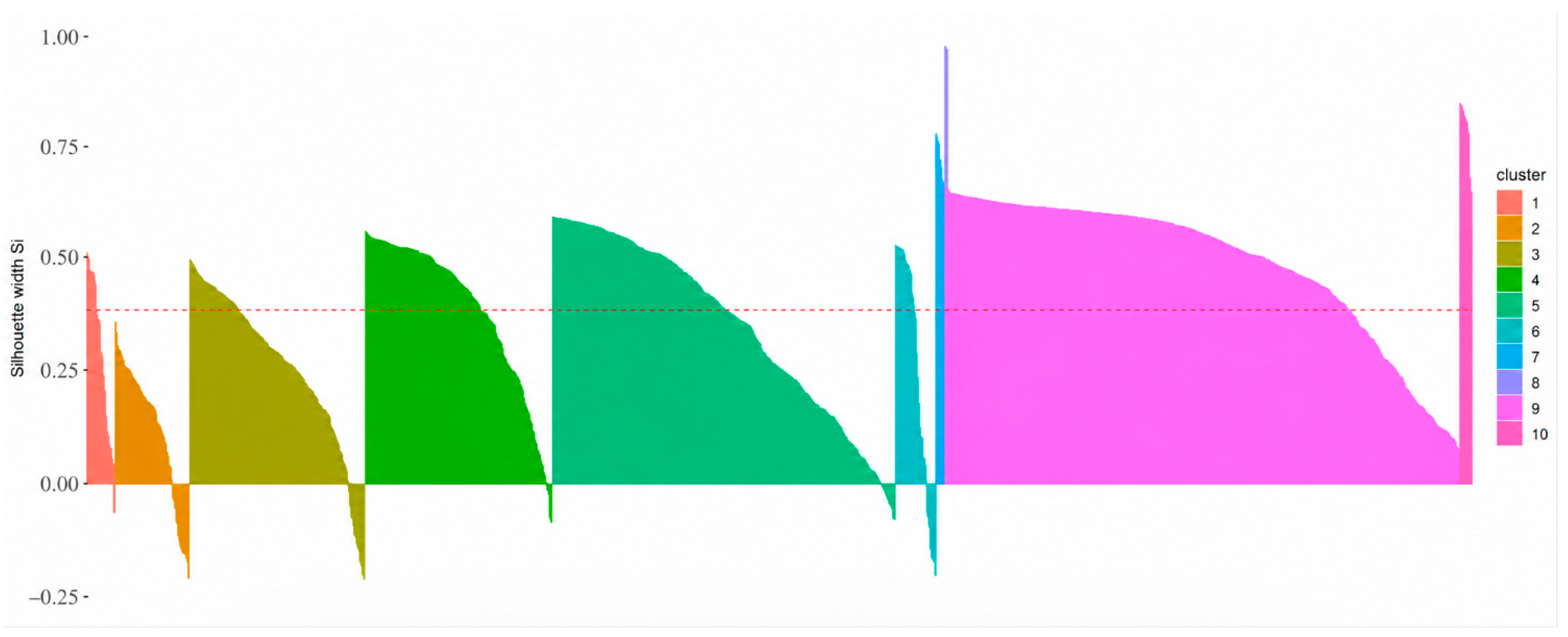
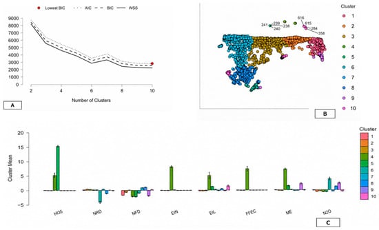
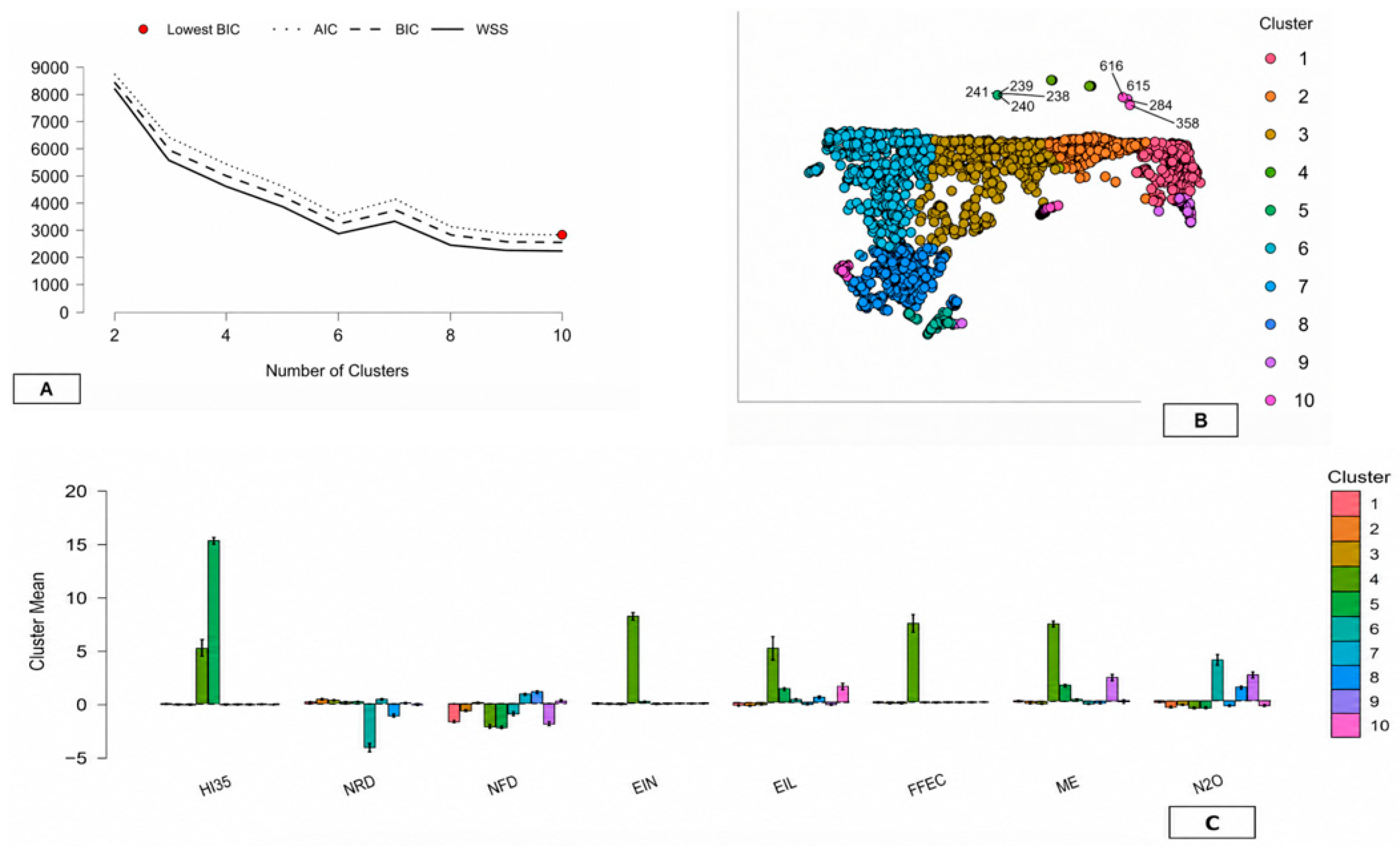
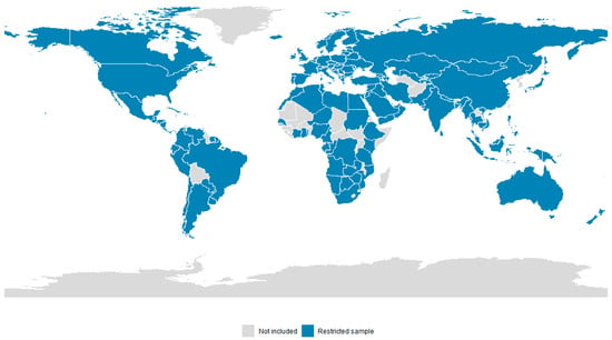
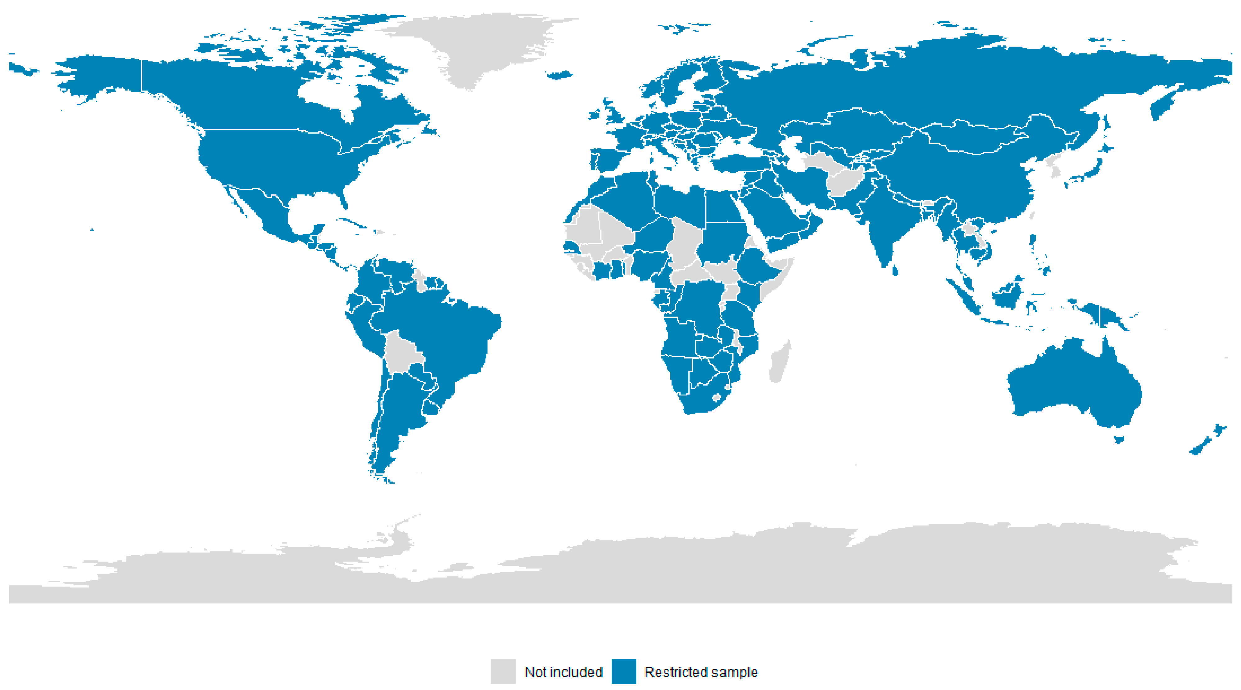
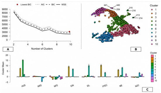
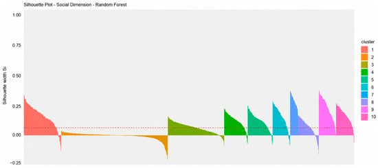
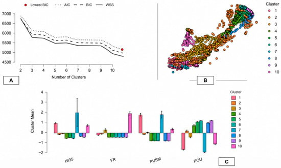
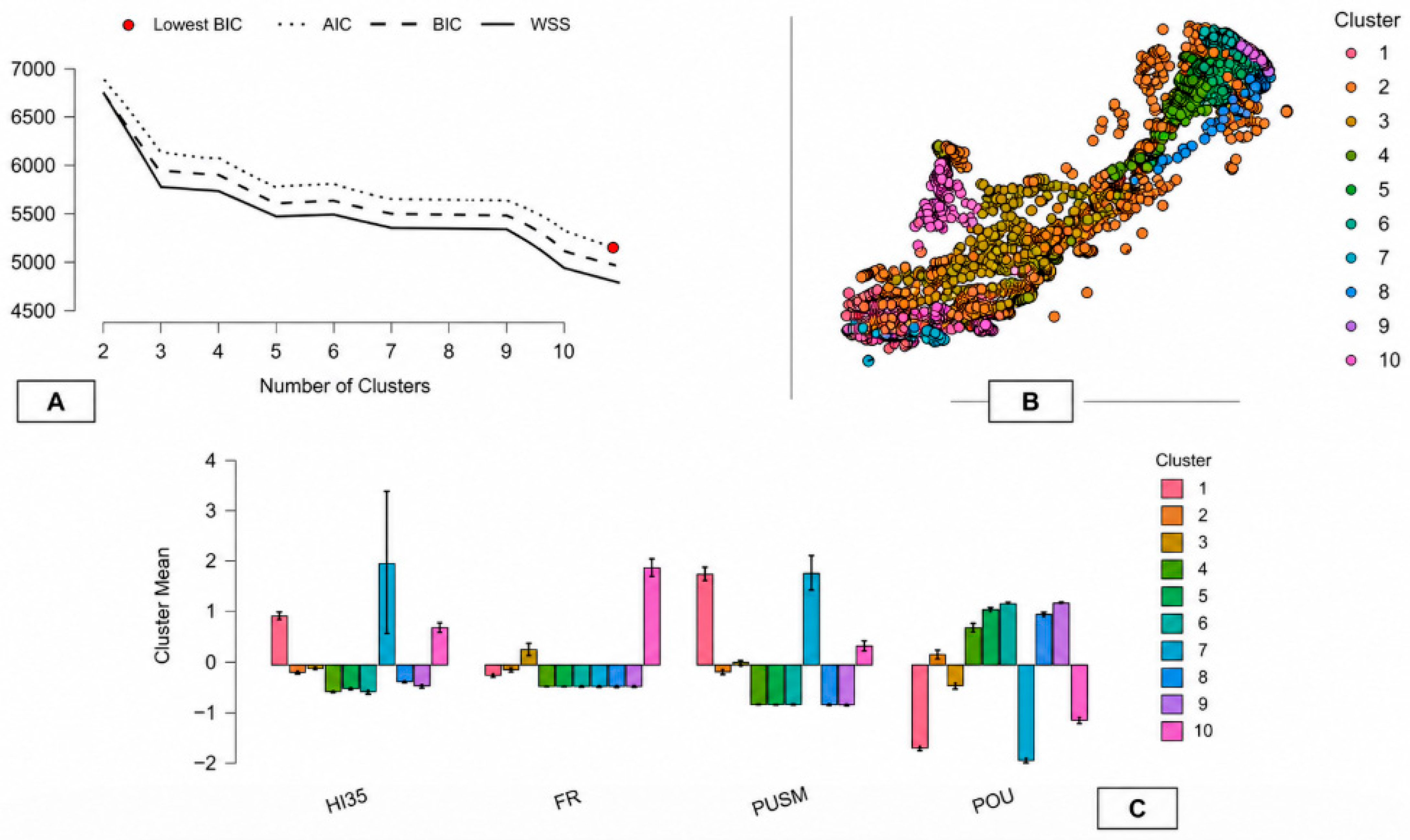
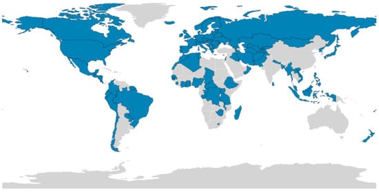
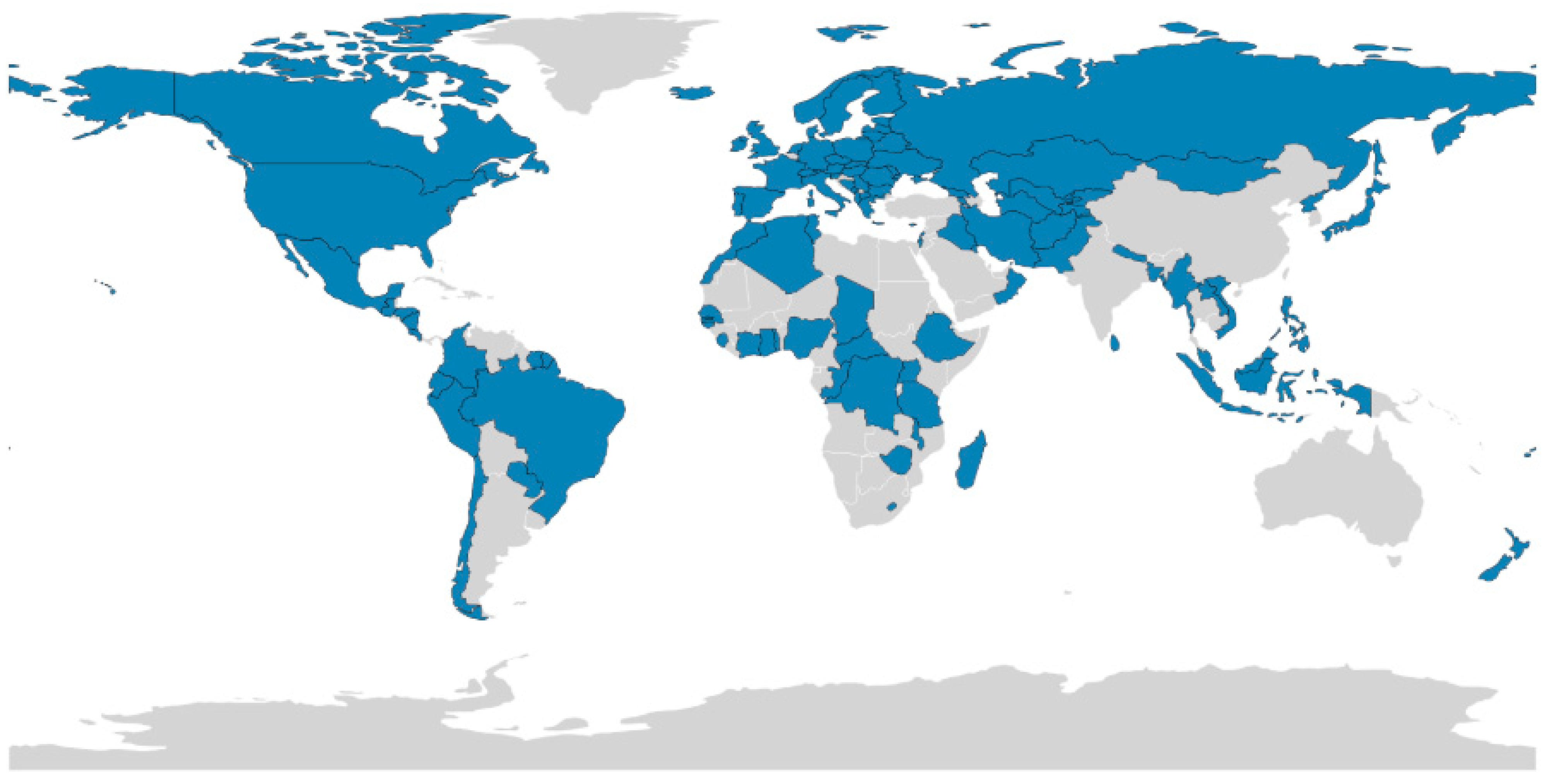
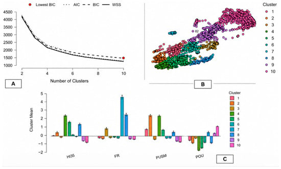
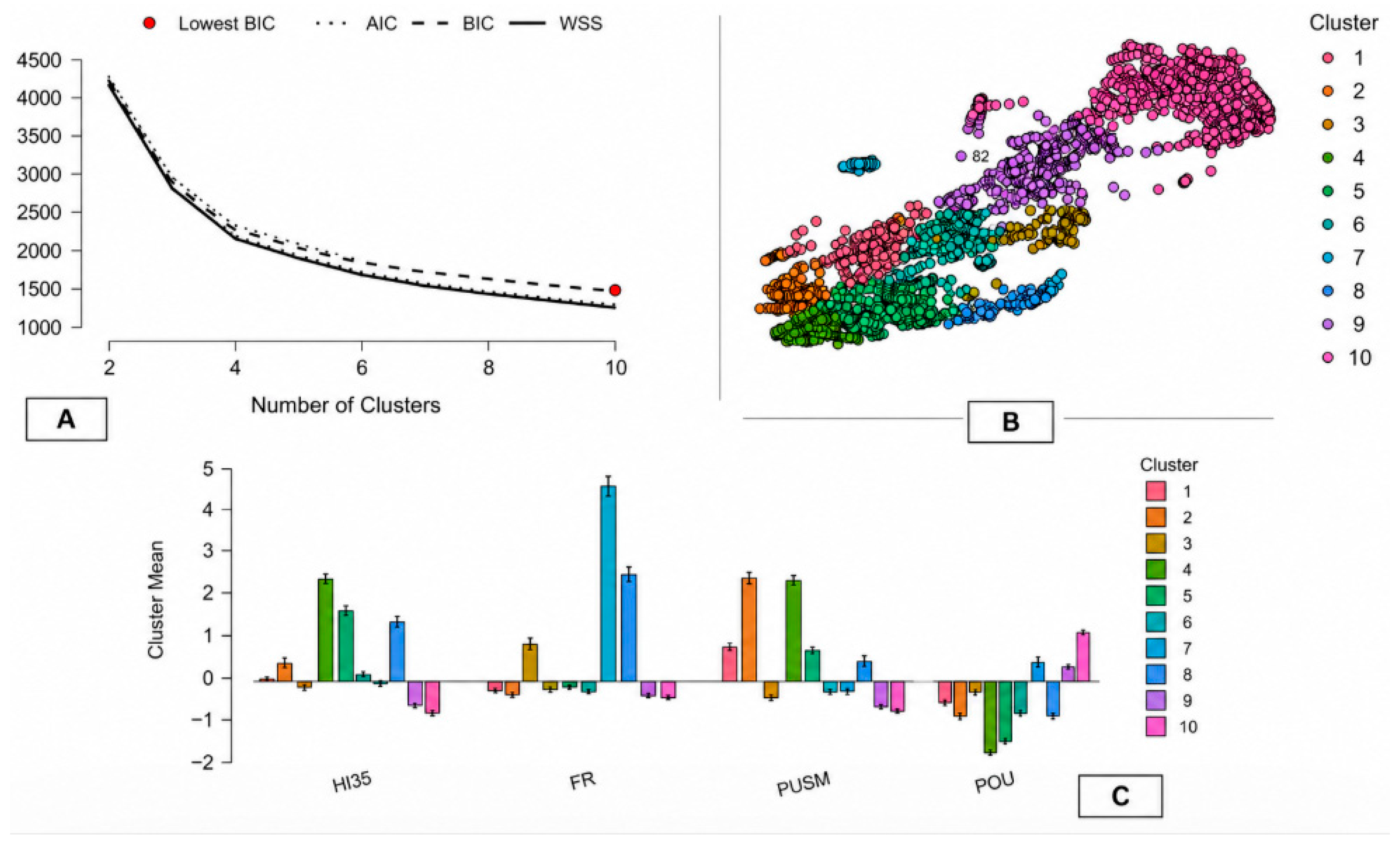
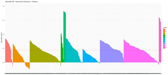
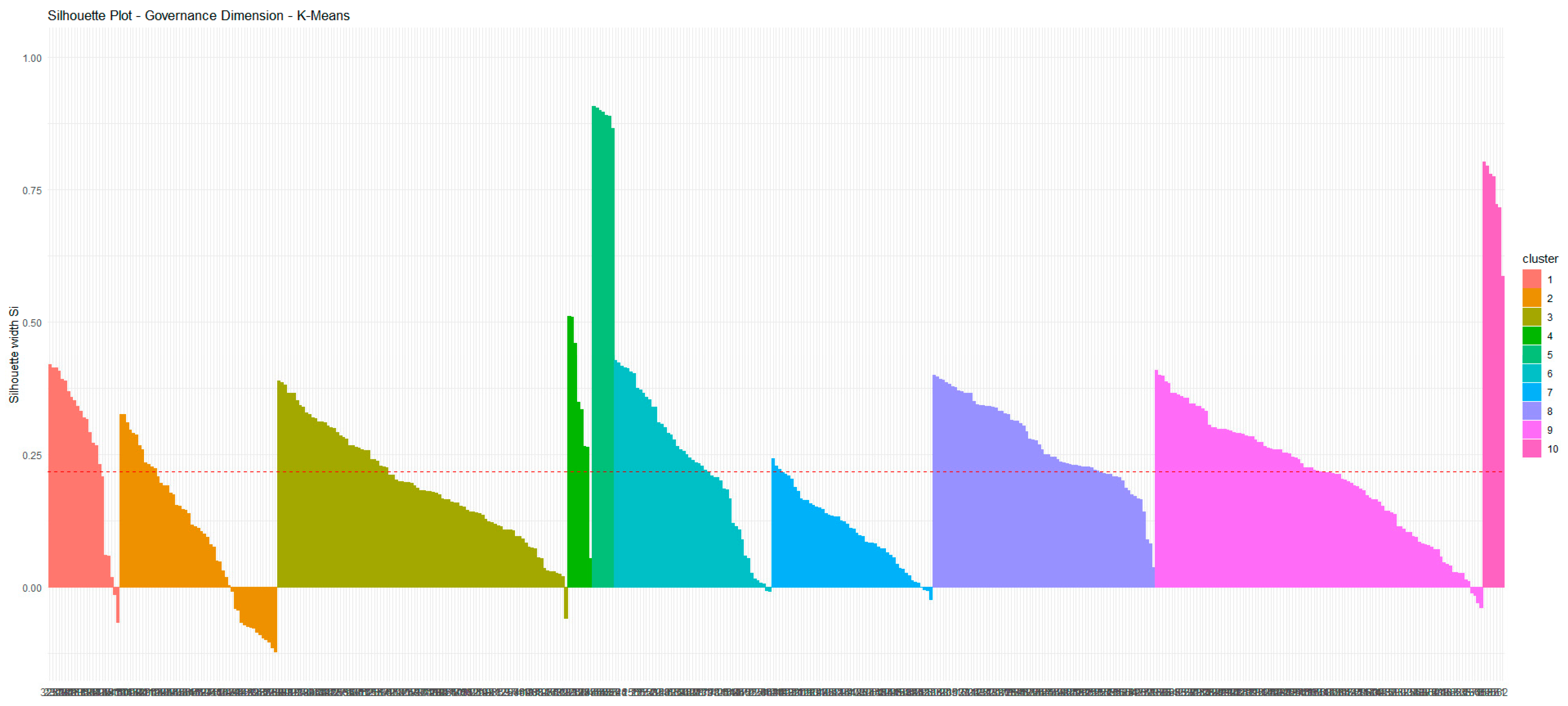
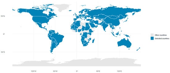
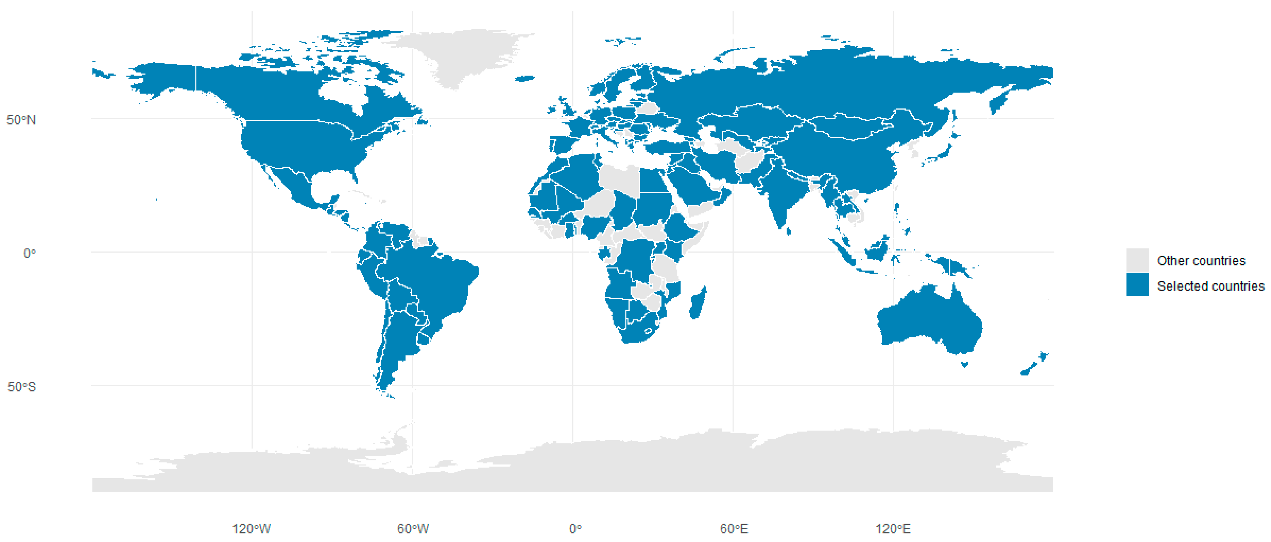
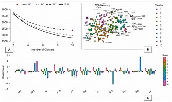
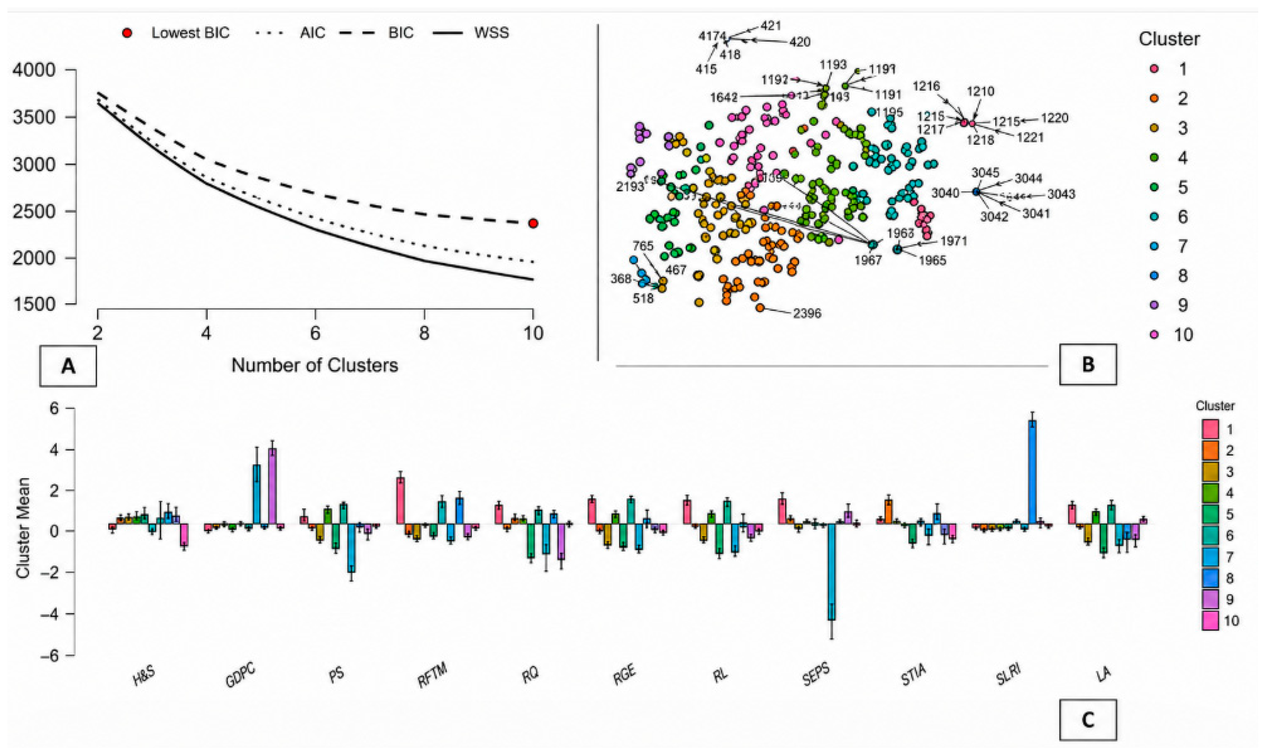
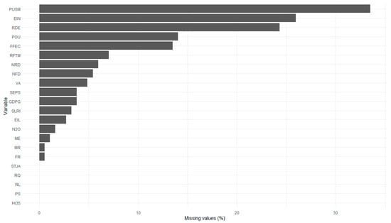
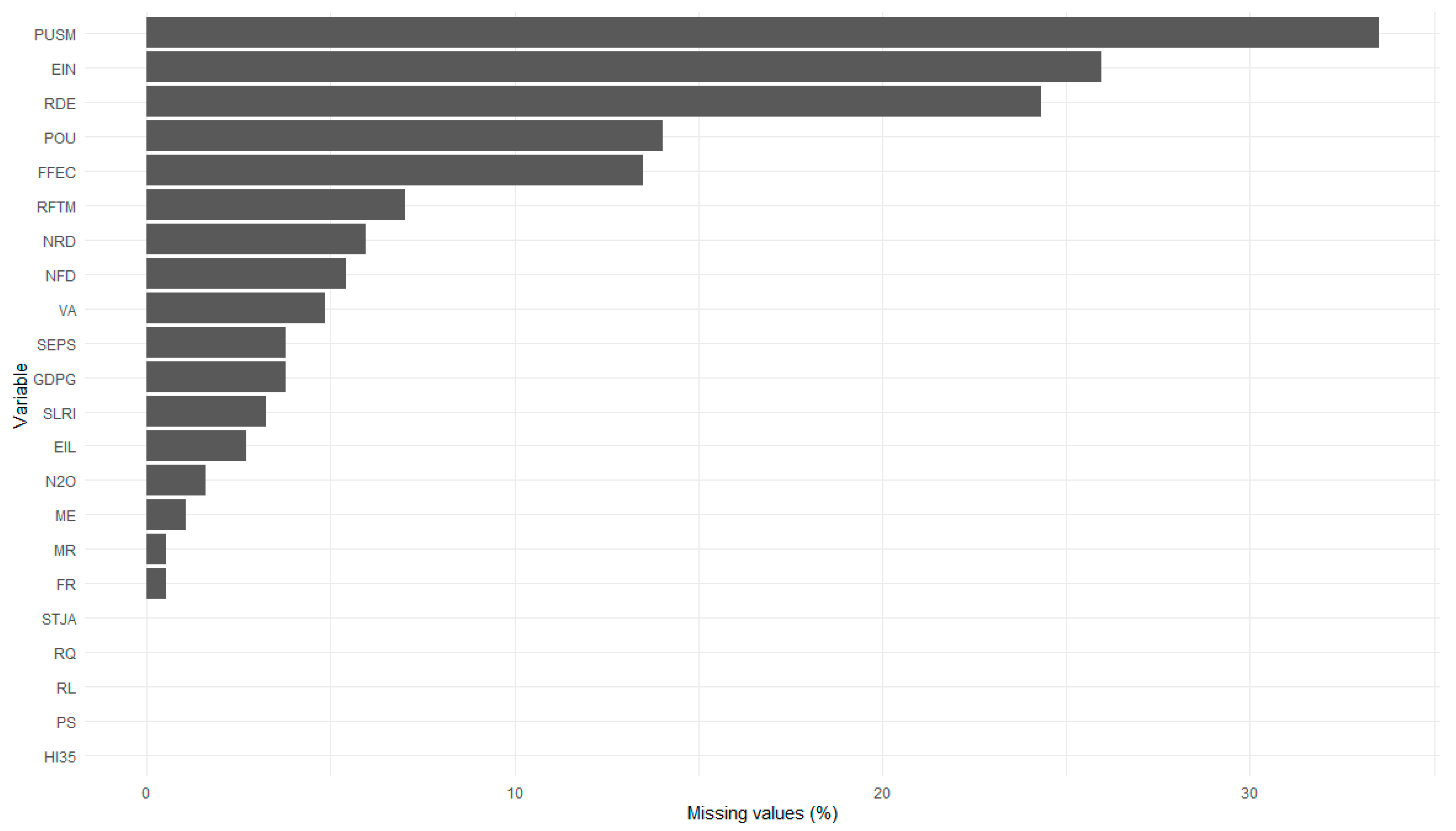
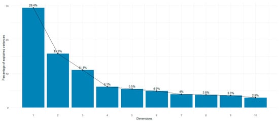
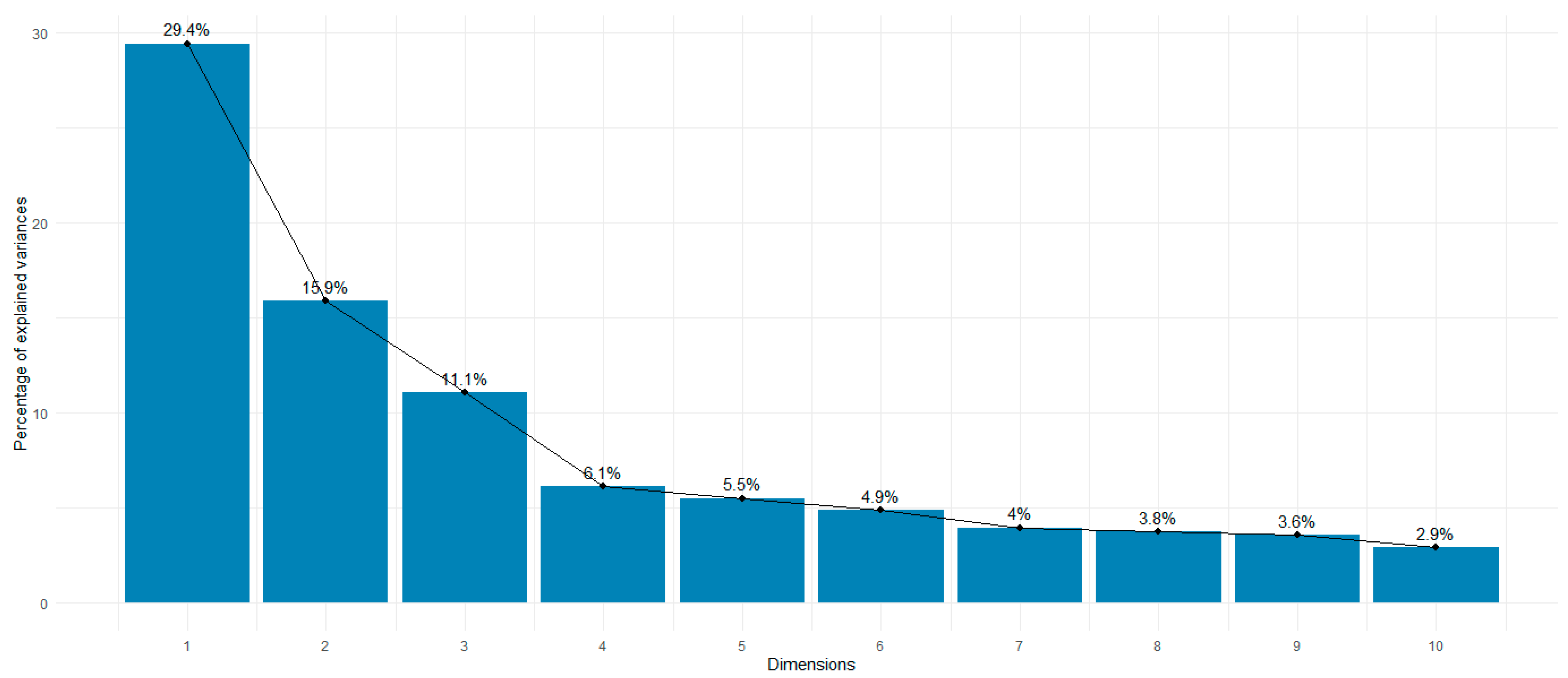
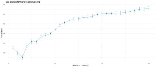
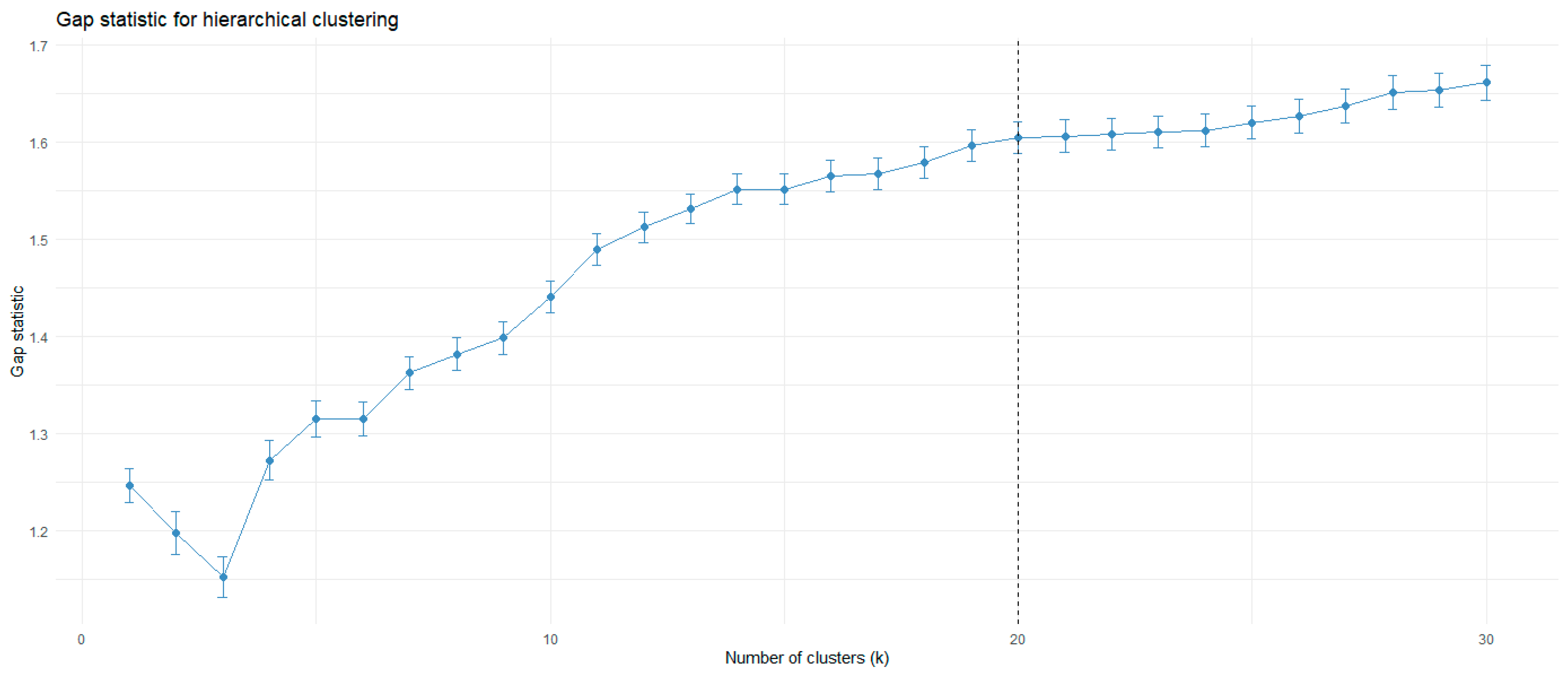
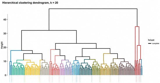
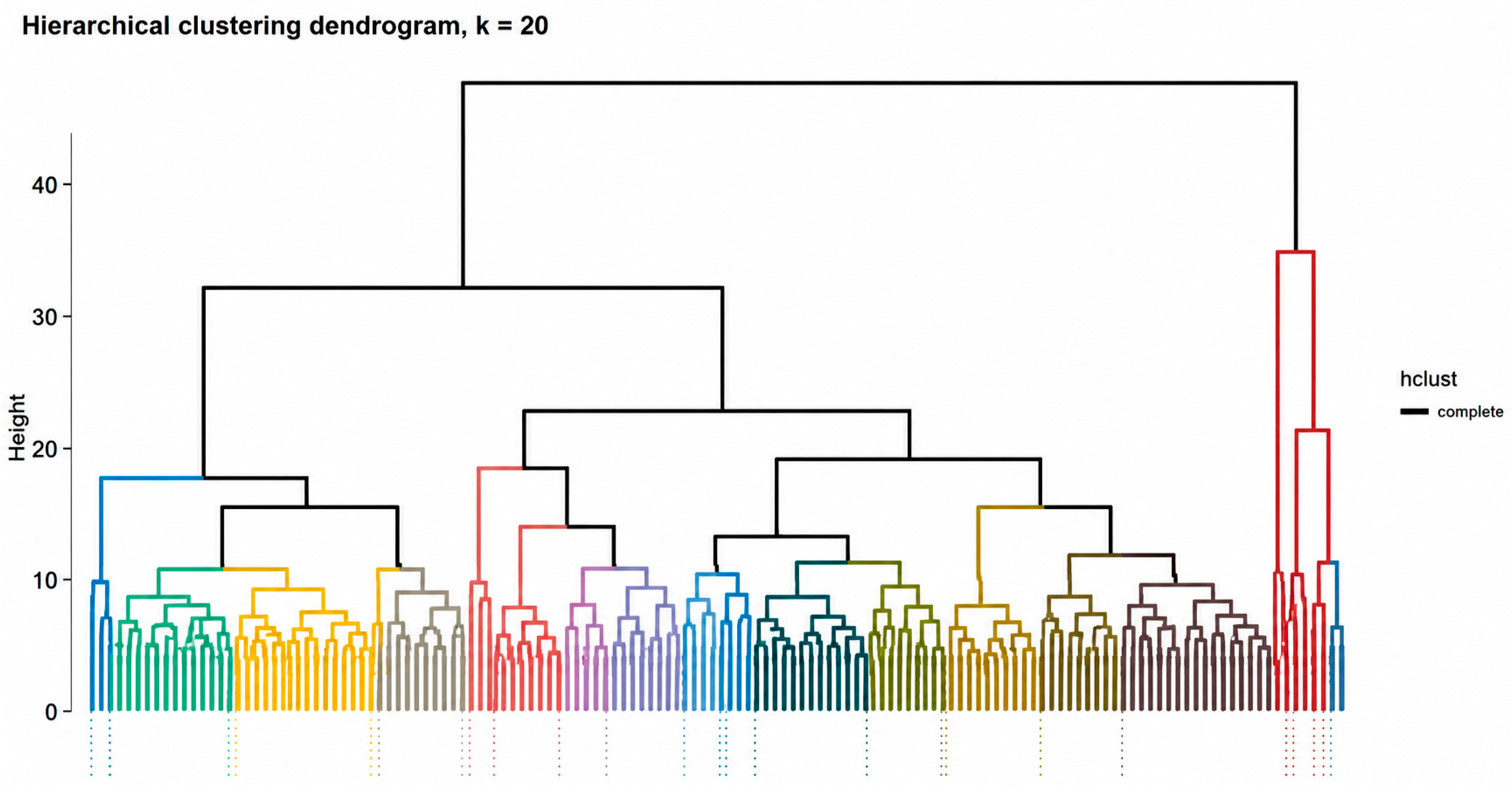
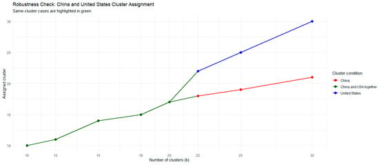
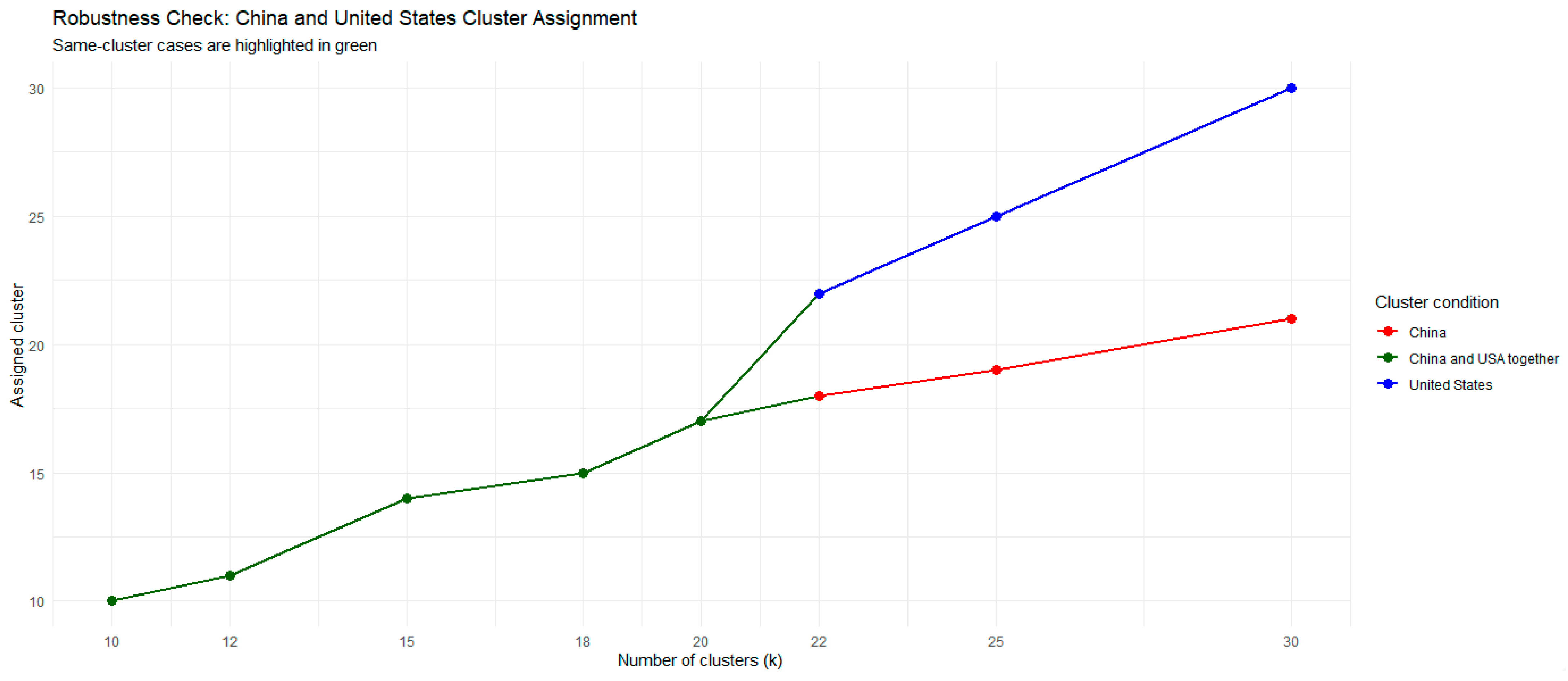
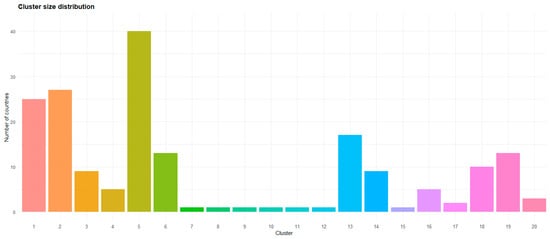
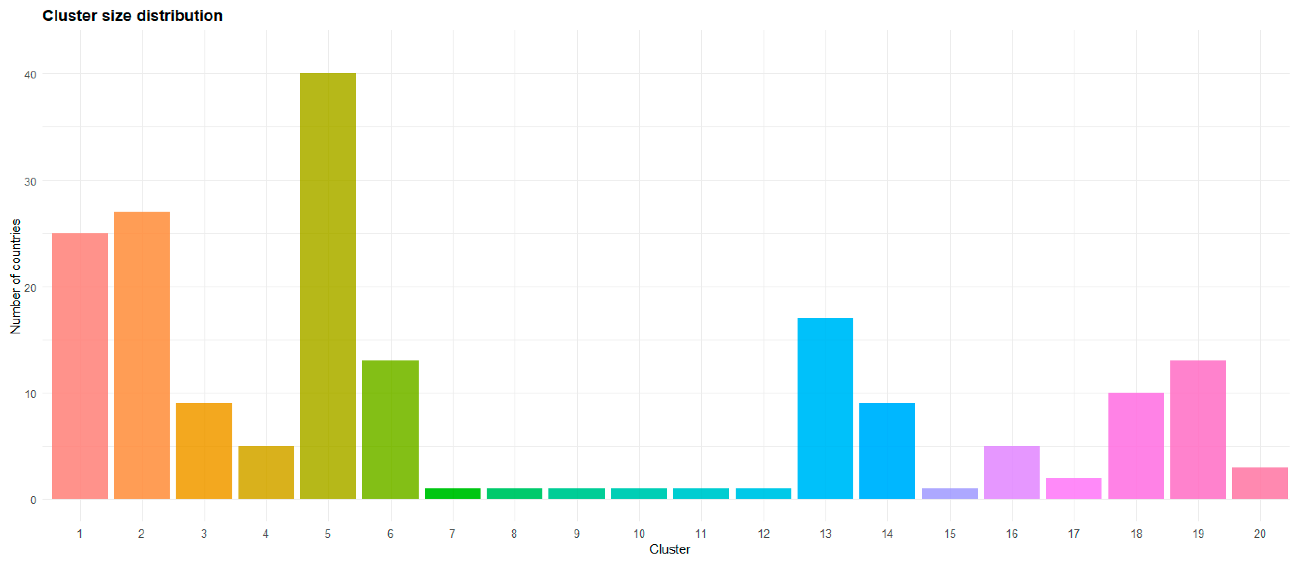

Disclaimer/Publisher’s Note: The statements, opinions and data contained in all publications are solely those of the individual author(s) and contributor(s) and not of MDPI and/or the editor(s). MDPI and/or the editor(s) disclaim responsibility for any injury to people or property resulting from any ideas, methods, instructions or products referred to in the content. |
© 2026 by the authors. Licensee MDPI, Basel, Switzerland. This article is an open access article distributed under the terms and conditions of the Creative Commons Attribution (CC BY) license.