


Abstract
Integrating spatial temperature and modeled health data requires compatible geographic units and valid treatment of prevalence estimates. This Houston-area study audits an intersected dataset and examines the sensitivity of its tract-level associations. Thirty health-prevalence fields exhibited an apparent multiplicative scaling pattern with record-specific factors. Reconstruction recovered 740 source tracts, including 659 under strict quality criteria. Identifier agreement was 434/435 (99.8%) in the directly checkable subset, not validation of all records; 642 assignments remained inferred, and the findings are conditional on the reconstructed crosswalk. Excluded tracts were cooler and less socially vulnerable. The reported land surface temperature (LST) field averaged 80.83 °F (27.13 °C); it was derived from Landsat 8 imagery acquired on 27 September 2022 using single-channel processing in ArcGIS Pro. This early-autumn observation is distinct from peak-summer or long-term heat exposure. LST had weak positive correlations with lack of health insurance (r = 0.199) and overall social vulnerability (r = 0.171). After adjustment for social vulnerability and tract share aged 65 years or older, standardized LST coefficients were 0.014 for lack of health insurance, −0.088 for obesity, −0.140 for current asthma, and −0.115 for stroke. In an eight-neighbor spatial-error specification, corresponding coefficients were 0.058, 0.021, −0.002, and −0.021; confidence intervals included zero for all three chronic-disease outcomes. Sensitivity analyses demonstrate that geographic selection, age composition, and spatial dependence materially affect interpretation. The principal contribution is the reproducible audit of the archived table; these ecological results do not establish heat-related disease risk or a validated basis for intervention targeting.
1. Introduction
1.1. Urban Surface Heat and Public Health
Extreme heat is an important climate and public-health hazard, particularly in growing metropolitan regions where warming interacts with dense development and extensive paved surfaces [1,2,3,4]. Urban thermal conditions depend on land cover, building materials, urban geometry, vegetation, soil moisture, and anthropogenic heat [5,6]. These processes create temperature differences over short distances that a single meteorological station may not capture. The built environment therefore contributes to variation in heat exposure and associated health burdens [1,5,6,7].
Land surface temperature (LST) is the radiometric temperature of roofs, pavement, vegetation, soil, and other surfaces observed by a remote sensor [8]. It differs from near-surface air temperature and individual thermal exposure [8,9]. MODIS and ECOSTRESS observations can reveal spatial contrasts relevant to heat-vulnerability assessment [10]. However, exposure also depends on humidity, wind, shade, indoor conditions, cooling access, activity, and time outdoors [4,11,12]. Interpreting an LST layer therefore requires documentation of its acquisition and processing.
1.2. Environmental Justice and Neighborhood Heat Inequality
Heat exposure and adaptive capacity are socially patterned. Housing quality, air-conditioning access, energy affordability, transportation, occupation, social isolation, pre-existing illness, and healthcare access influence residents’ ability to avoid or recover from heat [11,12,13,14]. Across U.S. cities, lower-income and racial and ethnic minority populations often experience greater surface-heat exposure [13,15,16,17]. Historical housing discrimination and unequal investment in vegetation, infrastructure, and public amenities contribute to these disparities [13,15,17,18].
Heat-vulnerability frameworks commonly distinguish exposure, population sensitivity, and adaptive capacity [19,20,21,22,23]. The 2020 CDC/ATSDR Social Vulnerability Index (SVI) summarizes socioeconomic status, household composition and disability, minority status and language, and housing type and transportation [24]. SVI can describe social conditions relevant to heat preparedness, but it is not a direct measure of heat exposure or disease risk. Its relationship with modeled health estimates also requires attention to shared demographic and socioeconomic inputs.
1.3. Houston as a Climate–Health Case
Houston provides a relevant setting because its hot–humid climate, extensive development, and uneven vegetation create contrasting thermal and social environments [25,26]. Houston-focused modeling shows that prioritizing social vulnerability changes the distribution of proposed heat-mitigation benefits [27]. Local research also distinguishes cooler vegetated vacant parcels from warmer abandoned structures and paved surfaces [28]. These studies motivate careful spatial data integration. Houston’s climate normals provide regional context only. The 27 September 2022 Landsat 8 acquisition [28] is distinguished from peak-summer conditions and from long-term ambient or personal heat exposure.
1.4. Research Gaps, Data Challenge, and Objectives
Several challenges arise when environmental layers are combined with small-area health estimates. LST does not measure the same exposure as air temperature, while chronic-disease prevalence differs from heat-related hospitalization or mortality [1,7,11,23]. Index rankings depend on indicator selection, weighting, and geographic scale [19,20,21,22,23]. PLACES estimates are modeled using demographic and socioeconomic information, making secondary adjustment for related variables difficult to interpret [29,30]. Spatial dependence further complicates ecological associations [31]. A prior requirement is that values remain valid when datasets with different geographic units are combined.
The primary objective is to audit and document the recovery of health-prevalence fields in an author-provided Houston-area project dataset. A secondary objective is to assess how reconstructed associations change with sample selection, age adjustment, SVI specification, and spatial-error modeling. The study therefore (1) examines proportional scaling of health fields and source-tract recovery; (2) evaluates identifier agreement, geographic plausibility, and exclusion patterns; (3) compares standardized global coefficients across a limited set of diagnostic specifications; and (4) assesses local smoothing and a simplified temperature–SVI co-location score. These analyses support a methodological assessment of the dataset rather than an estimate of heat-related disease risk.
2. Literature Review
2.1. Urban Heat Exposure and Health Pathways
Global research documents increasing urban exposure to extreme heat and a contribution of human-induced climate change to heat-related mortality [2,3]. Regional warming establishes the broader context, while urban land cover and social conditions influence local exposure and adaptive capacity [4,5,6]. These findings motivate neighborhood-scale analysis without establishing that every available surface-temperature snapshot represents a relevant period of hazardous heat.
Heat-related health effects involve thermoregulation, dehydration, cardiovascular strain, respiratory stress, and renal injury [1,4,5,7,12,32]. Epidemiologic evidence links heat exposure with adverse health outcomes, including cardiovascular morbidity among older adults [1,7]. Air pollution can coincide with high temperatures and complicate attribution [5]. Such evidence supports studying heat-sensitive populations, but cross-sectional modeled prevalence cannot be interpreted as a direct measure of illness caused by a particular temperature observation.
Protective responses depend on access to cooling, energy, transportation, and medical care [11,12]. Lack of health insurance among adults aged 18–64 years is one relevant access indicator. It is used here under its specific measure name, rather than as a comprehensive measure of healthcare access; it does not capture provider availability, affordability among insured residents, transportation, or trust in services.
2.2. Remote Sensing and Neighborhood Thermal Exposure
Satellite LST offers spatial coverage across urban surfaces that sparse meteorological networks cannot provide [8,10]. ECOSTRESS and MODIS illustrate its value for identifying spatial thermal contrasts [10]. Interpretation depends on spatial resolution, observation time, cloud screening, emissivity, and aggregation. A tract mean may have less variation than its constituent pixels, and its distribution alone cannot identify the sensor or processing product.
Surface and near-surface air temperatures may differ in both magnitude and spatial pattern [9]. Humidity, wind, shade, mean radiant temperature, and indoor exposure also affect human thermal conditions [4,11,12]. Consequently, the archived temperature field can support an audit of the supplied table and conditional spatial description, but the single-date, early-autumn observation described in Section 3.3 does not establish peak-summer exposure or a long-term heat burden.
Land function also matters: vegetated parcels may support cooling, whereas roofs and pavement can retain heat. Ren et al. [28] examined vacant and abandoned land in Houston using Landsat-derived tract temperatures and separate drone thermal observations. That article also documents the Landsat acquisition and broad processing methods associated with the source study identified by the authors for the present temperature field. The current analysis concerns integration with PLACES health estimates and SVI; it does not reuse the earlier study’s drone observations as tract-level exposure data or reproduce its land-use models.
2.3. Environmental Justice and Adaptive Capacity
Urban heat exposure varies with social and historical conditions. U.S. studies report disparities by income and race or ethnicity [15,16,17], while research across 108 urban areas associates historical redlining with contemporary surface-temperature differences [18]. Unequal distributions of tree canopy, parks, infrastructure, and impervious surfaces provide plausible pathways. These findings justify an environmental-justice perspective without implying that this dataset identifies the mechanisms producing local health inequalities.
Health vulnerability combines exposure with physiological sensitivity and adaptive capacity. Reviews identify socioeconomic and built-environment conditions as relevant to that relationship [6,13,14]. Neighborhoods with similar temperatures can differ in housing, cooling access, occupation, transportation, and baseline health. Age composition is especially important when outcomes are crude prevalence estimates rather than age-standardized disease rates.
The feasibility of mitigation also varies across places. Houston modeling and comparative research in Alabama show that social vulnerability, land availability, and local context influence proposed responses [20,27]. Trees, reflective roofs, shade, cooling facilities, and health outreach require different implementation resources [11,12,27]. Ecological co-location maps can support discussion, but operational targeting requires validated exposure information and local assessment.
2.4. Heat-Vulnerability Indices and Small-Area Health Data
Reviews of heat-vulnerability indices show substantial differences in indicators, normalization, weighting, validation, and spatial units [19,23]. Rankings can change when correlated measures are added or geographic coverage changes. An index containing both SVI and SVI-correlated health estimates may count similar social information more than once. Correlations among index components should be examined to assess potential redundancy.
Studies in Southeast Florida and research integrating remote sensing with machine learning demonstrate different approaches to combining exposure, sensitivity, and adaptive capacity [21,22]. Their relevance here is the importance of explicit indicator definitions and assumptions. The predictive value of these indices depends on input quality and validation against heat-related outcomes.
CDC PLACES uses multilevel regression and poststratification to generate small-area health estimates [29,30]. Its demographic and socioeconomic inputs overlap conceptually with variables summarized by SVI. A high fit between SVI and PLACES outcomes can therefore reflect shared estimation structure as well as geographic co-patterning. The conditional models in this study are treated as specification diagnostics, not independent epidemiologic validation; age adjustment does not remove all such dependence.
2.5. Spatial Dependence and Non-Stationarity
Spatially clustered exposures and health estimates can leave correlated residuals in conventional regression. Global Moran’s I assesses overall spatial autocorrelation [33]. Spatial-error models explicitly represent dependence in the disturbance term [34], whereas GWR estimates local coefficients and can act as a spatial smoother. GWR guidance requires attention to bandwidth selection, local collinearity, residual structure, and interpretation [35,36]. Better local fit alone does not demonstrate a distinct geographic mechanism.
Recent spatial analysis of urban heat and coronary heart disease illustrates the importance of comparing conventional and spatial specifications [31]. For modeled tract-level outcomes, leaving one observation out does not remove correlated neighboring information. Accordingly, validation should be distinguished from within-region interpolation.
Rates, percentages, modeled prevalence, and percentile ranks are not additive counts. Apportioning them by area can preserve recognizable maps while introducing artificial shared variation. The methodological contribution of this study is to make that problem, its reconstruction assumptions, and its consequences for subsequent interpretation explicit.
3. Materials and Methods
3.1. Study Area and Analytical Unit
The analytical frame is the 1077 records in SVI2020_Houston_Combined_Centroids.csv from the author-provided HEAT_Houston project archive. Each record has a distinct supplied FIPS identifier, but its health profile may originate from an older PLACES tract. Reconstruction identifies 740 source tracts: 698 in Harris County, 30 in Fort Bend County, 10 in Montgomery County, and 2 in Brazoria County. The strict sample comprises 659 tracts: 626 in Harris, 24 in Fort Bend, and 9 in Montgomery; no Brazoria tract passes the strict filter. The sampling frame is defined by the archived layer, not the Houston municipal boundary or a complete metropolitan census. Supplementary Table S2 and Figure S1 show the county counts and spatial exclusions.
3.2. Data Sources and Variables
Table 1 summarizes the sources and analytical roles. LST_MEAN is the archived temperature field derived from Landsat 8 imagery acquired on 27 September 2022 and processed in ArcGIS Pro3.0.4 (Esri, Redlands, CA, USA) using a single-channel method. Section 3.3 describes the acquisition, processing approach, and remaining reproducibility requirements. Overall 2020 SVI (RPL_THEMES) and its four theme ranks describe social context [24]. The archived 2022 PLACES GIS-friendly file contains 30 prevalence fields and was checked against the public CDC release: all 156,660 compared prevalence cells across 5222 Texas records agreed. The four focal measures are lack of health insurance among adults aged 18–64 years (ACCESS2), and obesity, current asthma, and stroke among adults aged 18 years or older [29,30]. These are crude, modeled population estimates, not individual clinical records. The release uses 2020/2019 BRFSS data, 2010 Census population information, and 2015–2019 ACS covariates; the release year is not the observation year [30]. For age adjustment, the percentage aged 65 years or older was joined directly by source FIPS from the 2018 SVI database (2014–2018 ACS), which uses compatible source-tract geography [37]. This earlier age measure was available for all 659 strict-sample tracts. A sensitivity model replaces reaggregated 2020 SVI with directly joined 2018 SVI to assess dependence on the geographic crosswalk.
Table 1.
Data sources and analytical roles in the reconstructed tract-level analysis.
3.3. Land Surface Temperature
LST was derived from Landsat 8 imagery acquired on 27 September 2022 and calculated in ArcGIS Pro using the single-channel workflow described by Avdan and Jovanovska [38]. The author-supplied acquisition illustration identifies this date, and the converted LST and corresponding NDVI rasters are supplied as Extract_LST_22.lpkx and Extract_NDVI_22.lpkx. The related Houston study [28] provides additional study context. This manuscript uses the single-date Landsat input identified above.
The workflow uses thermal infrared Band 10 for radiance and brightness-temperature calculations and optical Bands 4 (red) and 5 (near infrared) to calculate NDVI = (Band 5 − Band 4)/(Band 5 + Band 4) [38]. NDVI is used to estimate vegetation proportion and land-surface emissivity, which is applied to the brightness temperature to obtain LST. These raster calculations were implemented in ArcGIS Pro; the cited paper originally implemented its algorithm in ERDAS IMAGINE. The paper provides the methodological basis, while scene-specific coefficients and the exact historical raster expressions must be established from the original processing records. Its example constants are not treated as recovered metadata for the Houston acquisition.
The supplied layer packages contain single-band, 32-bit raster datasets on matching 30 m grids, with 2942 columns and 2426 rows in WGS 84/UTM zone 15N (EPSG:32615). This is the stored raster cell size, not evidence of a native 30 m thermal measurement. The package layer definitions record version 2.9.0, which documents the packaging format rather than establishing the software version used for every calculation. Avdan and Jovanovska report LST in degrees Celsius [38]; the archived tract field LST_MEAN is retained in degrees Fahrenheit and converted for reporting using °C = (°F − 32)/1.8. The reported mean of 80.83 °F (27.13 °C), SD of 2.10 °F (1.17 °C), and tract range of 69.94–87.08 °F (21.08–30.60 °C) describe the existing archived-field analysis. The supplied raster packages do not preserve the complete unit-conversion and raster-to-tract processing history.
The analysis package includes the converted LST and NDVI layers, acquisition illustration, and methodological paper. The illustration lists land and scene cloud-cover values of 0.01, but does not identify their units or provide a pixel-level quality mask. The original Landsat band files and MTL scene metadata, product identifier, precise overpass time, cloud-mask implementation, and complete calculation and extraction logs remain unavailable. Consequently, the files support access to the processed layers and a more explicit method description, but not an independent reproduction of the original satellite retrieval or the exact archived LST_MEAN variable. The custom Band 10 workflow should not be identified as the USGS Collection 2 Level-2 temperature product solely on the basis of general product documentation [8].
3.4. Data-Integrity Audit and Reconstruction
The audit concerns a dataset in the authors’ project archive rather than an independently obtained third-party layer. The archived matching notebook, HEAT_a1_MatchData_20250925.ipynb, documents joining PLACES TractFIPS to GEOID in the Census cb_2015_48_tract_500k boundary file using ArcPy. It does not document the later operation that scaled the prevalence fields. The author-identified temperature input is the 27 September 2022 Landsat 8 acquisition, processed in ArcGIS Pro using the Avdan and Jovanovska workflow [38]. The converted LST and NDVI layers are now supplied, although the exact historical raster-to-tract settings and unit-conversion history are not preserved in the available notebook. Small health values with preserved multivariable proportions indicated a common scaling factor. Reconstruction identifies the source health profile and estimates this factor; it does not establish the original operator, software settings, or physical meaning of the factor. The following steps describe the existing archived-field analysis.
- Health-profile matching: The 30-field prevalence vector for each record and each complete Texas PLACES source record was normalized to unit length. Cosine similarity identified the closest profile. Candidates within 10−10 of the maximum similarity were treated as numerical ties and resolved by the shortest centroid distance. Using all 5203 complete Texas source profiles (of 5222 source records) avoids an undocumented regional candidate-selection boundary.
- Geographic checks: Matching used Euclidean distance in the supplied longitude and latitude coordinates for consistency with the original reconstruction thresholds. As an additional plausibility check, record centroids were tested for containment in the matched Census 2015 tract polygons, with coordinate transformation from WGS 84 to the boundary CRS, NAD83 (EPSG:4269). Polygon containment was not used to select the profile match and is supporting geographic evidence, not definitive validation of each intersected record.
- Scaling-factor estimation and source joins: For record vector a and matched PLACES vector b, the least-squares factor is the sum of ajbj divided by the sum of bj2. The four outcomes were taken directly from the matched public-source PLACES record without further scaling. Factors normalized within each recovered tract were used to reproduce weighted LST and SVI means. The resulting SVI values are interpolated summaries of 2020 ranks, not official 2020 ranks for the older source tracts. The supplied converted LST raster supports source inspection, but a direct FIPS join alone does not recover its historical extraction settings or resolve a change in tract geography; the 2018 SVI sensitivity model provides a compatible-geography social-data comparison [37].
- Quality filtering and sensitivity: The primary filter required a factor sum of 0.95–1.05, minimum similarity of 0.9999, and maximum centroid separation of 0.08 decimal degrees. Alternative lower factor-sum bounds were 0.85, 0.90, and 0.98; additional checks tightened similarity to 0.99999 and distance to 0.04 degrees. One threshold was changed at a time. An all-740-tract comparison was also reported, with explicit recognition of incomplete reconstruction. Standardized mean differences and descriptive distributions compared retained and excluded tracts, and directly checkable and non-checkable records. These comparisons assess selection, not the accuracy of every inferred assignment.
All 1077 records have supplied FIPS identifiers, but only 435 are directly comparable with a PLACES source identifier. Of these, 434 agree with the profile assignment (99.8%); 642 lack a directly comparable identifier rather than a FIPS value altogether. The checkable and non-checkable subsets differ materially, so 99.8% is not an accuracy estimate for the entire crosswalk. Polygon containment supported 424/435 assignments in the checkable subset and 628/642 in the remaining subset. These checks strengthen geographic plausibility while leaving source-assignment uncertainty, particularly where boundaries changed. The complete crosswalk and comparison statistics are included in the supplementary package. All statistical findings are conditional on this reconstructed crosswalk, whose inferred assignments affect sample membership and the associated LST and SVI values; the 99.8% agreement does not validate the full dataset.
3.5. Descriptive and Global Statistical Analysis
Descriptive statistics, Pearson correlations, and Spearman correlations were calculated for the strict sample. OLS specifications included LST alone; LST with overall SVI; and LST with SVI and tract share aged 65 years or older. A diagnostic model replaced overall SVI with its four themes while retaining age. The two SVI specifications were not combined in one model. HC3 standard errors describe heteroskedasticity-robust uncertainty conditional on the reconstructed table, but do not correct spatial dependence or propagate PLACES estimation or source-assignment uncertainty. Coefficients are reported as standardized associations, β = b × SD(LST)/SD(outcome), with percentage-point coefficients per 1 °F and per one LST SD retained in Supplementary Table S3. The strict-sample LST SD is 2.099 °F (1.166 °C). Global VIFs were calculated for every predictor; no coefficient is interpreted as a causal effect or an independently observed epidemiologic relationship.
3.6. Spatial Dependence and Diagnostic Model Comparisons
Global Moran’s I used row-standardized nearest-neighbor weights with k = 8, compared with k = 4 and 12 [33]. Neighbor sets were calculated in WGS 84/UTM zone 15N (EPSG:32615) after projecting factor-weighted record centroids. A fixed k avoids isolated observations in the incomplete sampling frame, although it imposes different physical distances in dense and sparse areas. We used 999 permutations and a fixed random seed; p = 0.001 is the smallest attainable pseudo-p value. The age- and SVI-adjusted OLS model was compared with a maximum-likelihood spatial-error model, y = Xβ + u and u = λWu + ε, using the same covariates and each weight matrix [34]. Residual diagnostics for that model refer to spatially filtered innovations ε. These model comparisons evaluate specification sensitivity rather than remove all exposure or outcome uncertainty.
GWR was retained solely as a diagnostic of the original two-predictor model, using standardized LST and overall SVI, an adaptive bisquare kernel, and bandwidths of 35, 45, 55, 70, 90, 120, 160, and 220 observations, including the focal observation. For each bandwidth, the fitted-value matrix S yields residuals e and leave-one-out residuals ei/(1 − Sii), with the kernel held fixed. LOOCV R2 = 1 − Σ[ei/(1 − Sii)]2/Σ(yi − ȳ)2; the minimum PRESS selected the bandwidth. We report the entire bandwidth comparison, AICc, local condition numbers, local predictor VIFs, and residual Moran’s I [35,36]. These calculations were rerun in the documented projected CRS. LOOCV describes local interpolation among spatially related, modeled outcomes and is not independent geographic validation. No MGWR, spatial Durbin, or spline models were added. Analysis used Python 3.11.11 with NumPy 2.3.5, pandas 3.0.5, SciPy 1.17.0, statsmodels 0.15.0, libpysal 4.15.0, esda 2.10.0, spreg 1.9.1, and pyproj 3.8.0; scripts and exact settings accompany the Supplementary Data.
3.7. Temperature and Social Vulnerability Co-Location Score
The earlier three-component index was audited for redundancy, then replaced by the mean of within-sample LST and overall-SVI percentile ranks. Health outcomes are excluded from the revised score. Thus, positive scoring no longer assumes that higher crude prevalence implies a stronger temperature–disease relationship, and the same social information is less likely to enter through both SVI and modeled health. Spearman rank correlations compare the original and revised scores with SVI alone. Average ranks divided by the sample size define percentiles, including ties. The score describes relative co-location of the reported temperature field and social vulnerability; it is not a validated heat-risk score or an intervention-allocation rule [19,23].
4. Results
4.1. Data Audit and Reconstructed Analytical Sample
The 1077 archived records were associated with 740 source tracts; this reduction is due to aggregation, not exclusion of 337 tracts. The median inferred factor was 0.701 (interquartile range, 0.405–0.993). Directly checkable records had a median factor of 0.995, compared with 0.467 among the remaining records, demonstrating that the 99.8% identifier agreement applies disproportionately to less-scaled cases. The strict filter retained 659/740 source tracts (89.1%), represented by 968/1077 archived records (89.9%). It excluded 81 source tracts, not approximately 35% of the original sample. Retained tracts had a mean LST of 80.83 °F (27.13 °C) versus 79.48 °F (26.38 °C) among excluded tracts, and a mean SVI of 0.568 versus 0.440. Standardized mean differences were 0.541 and 0.435, respectively. Exclusions were therefore systematic with respect to observed variables (Supplementary Tables S1 and S2). Figure 1 illustrates the common scaling pattern, and Table 2 summarizes reconstruction and sample retention.
Figure 1.
Reproduced data-integrity audit. (a) Estimated common factors for 1077 records. (b) Archived apportioned values versus directly joined PLACES lack-of-health-insurance estimates; the dashed line indicates equality. The estimated factors describe numerical scaling and do not establish the undocumented geoprocessing operation.
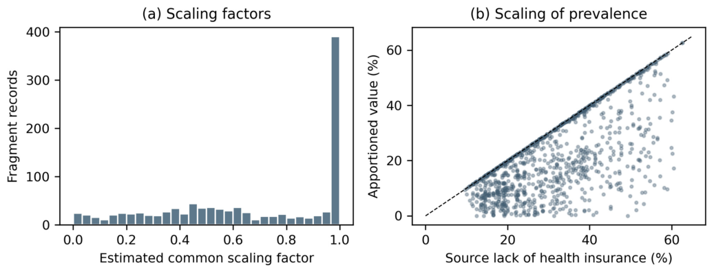
Table 2.
Data-integrity audit and sample reconstruction.
The term “earlier exploratory analysis” refers to the archived HEAT_Houston notebooks that analyzed the apportioned health fields before the source-profile audit. LASSO, Random Forest, correlation, VIF, GWR, spatial-lag, and spatial-error outputs based on those fields are not substantive results of the revised paper. They document the analytical consequences of invalid inputs, rather than findings from a separate published manuscript.
4.2. Descriptive and Spatial Patterns
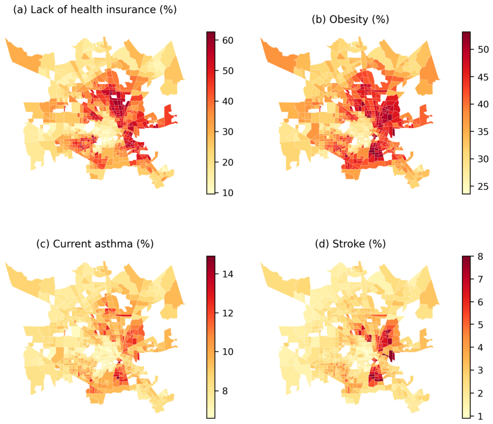
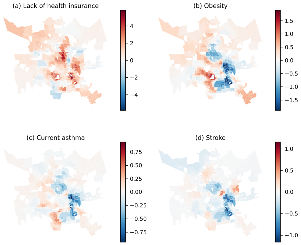
Mean reported LST was 80.83 °F (27.13 °C), ranging from 69.94 °F (21.08 °C) to 87.08 °F (30.60 °C). Overall reaggregated SVI averaged 0.568. Lack of health insurance ranged from 9.6% to 62.7%. The directly joined share aged 65 years or older averaged 10.51% (SD 5.11 percentage points), and was inversely correlated with LST (r = −0.244). These distributions characterize the retained sampling frame and do not verify the temperature product’s acquisition conditions. Table 3 summarizes these distributions; Figure 2 maps LST and SVI, and Figure 3 maps the four PLACES measures.
Table 3.
Descriptive statistics for the strict reconstructed tract sample.
Figure 2.
Reconstructed tract-level distributions of (a) LST derived from Landsat 8 imagery acquired on 27 September 2022 using single-channel processing in ArcGIS Pro and (b) factor-weighted 2020 SVI. LST represents a single early-autumn observation. SVI values are interpolated summaries, not official ranks for the older source geography. White gaps mark areas outside the retained sample.
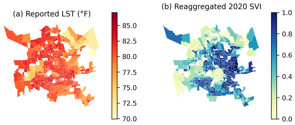
The mapped variables were spatially clustered in the original analysis. The revised inferential assessment concentrates on whether residual spatial dependence remains after adding age and whether conclusions change with the neighborhood definition (Section 4.4 and Supplementary Table S5). Spatial clustering by itself does not establish a temperature–health mechanism.
Figure 3.
Directly joined 2022 PLACES crude-prevalence estimates: (a) lack of health insurance among adults aged 18–64 years; (b) obesity; (c) current asthma; (d) stroke among adults aged 18 years or older. All maps use the strict reconstructed source-tract sample.
4.3. Bivariate and Global Regression Results
LST had weak positive correlations with lack of health insurance (Pearson r = 0.199) and overall SVI (r = 0.171). Obesity had a small positive correlation (r = 0.066), current asthma was near zero (r = −0.012), and stroke had a weak inverse correlation (r = −0.079). Table 4 retains conventional correlation p values for transparency; spatial dependence limits their interpretation as independent-observation tests. Table 5 compares standardized LST coefficients across global specifications, and Figure 4 shows the corresponding interval estimates.
Table 4.
Correlations between mean LST and social or health indicators (N = 659).
Table 5.
Standardized LST coefficients across OLS and spatial-error specifications (N = 659). Values are β (95% CI), in outcome SDs per one LST SD. OLS intervals use HC3; spatial-error intervals use model-based maximum-likelihood standard errors. SVI and age denote overall reaggregated 2020 SVI and directly joined tract share aged 65 years or older. Full coefficients, p values, and fit statistics appear in Supplementary Table S3.
Figure 4.
Standardized LST coefficients with 95% intervals: LST-only OLS, SVI-adjusted OLS, SVI-and-age-adjusted OLS, and the corresponding eight-neighbor spatial-error model. Intervals do not propagate PLACES or reconstruction uncertainty. These estimates describe specification sensitivity rather than individual or causal effects.
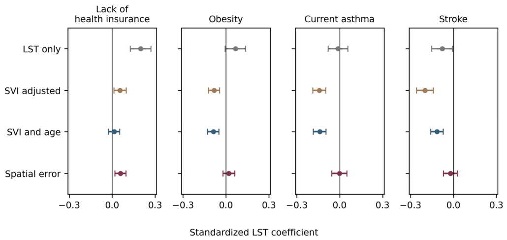
The SVI-adjusted standardized LST coefficient was 0.055 for lack of health insurance, −0.082 for obesity, −0.142 for current asthma, and −0.199 for stroke. Adding age changed these coefficients to 0.014 (95% CI −0.026 to 0.054), −0.088 (−0.127 to −0.049), −0.140 (−0.184 to −0.095), and −0.115 (−0.159 to −0.071), respectively. Thus, age adjustment reduced the stroke association and removed conventional statistical evidence for the small positive lack-of-health-insurance association in OLS. It did not eliminate the inverse obesity or asthma coefficients. Neither those coefficients nor their p values demonstrate protective effects of higher temperature.
Replacing overall SVI with its four themes and retaining age produced standardized coefficients of 0.021, −0.082, −0.134, and −0.112 for the four outcomes in the same order. Global VIFs were 1.030 for the original LST–SVI model and 1.078–1.122 after adding age; the largest VIF in the theme model was 5.484 for socioeconomic status. Thus, strong global collinearity between LST and overall SVI does not explain the original fit increase. Shared PLACES–SVI estimation inputs and spatial patterning remain distinct concerns. Results were similar across the 659- and 700-tract samples: age-adjusted standardized coefficients in the latter were 0.008, −0.087, −0.133, and −0.107. Complete threshold and compatible-geography SVI comparisons are provided in Supplementary Tables S3 and S4.
4.4. Residual Spatial Dependence and Local Variation
After adjustment for age and SVI, OLS residual Moran’s I remained 0.349–0.418 for k = 8 and 0.319–0.481 across k = 4, 8, and 12 (all permutation p = 0.001). HC3 covariance estimation does not correct this dependence. In the eight-neighbor spatial-error model, standardized LST coefficients were 0.058 (95% CI 0.020 to 0.097) for lack of health insurance, 0.021 (−0.021 to 0.062) for obesity, −0.002 (−0.055 to 0.051) for current asthma, and −0.021 (−0.070 to 0.028) for stroke. The three chronic-disease intervals included zero at all three neighborhood sizes. Lack of health insurance retained a small positive spatial-error coefficient, but its contrast with age-adjusted OLS demonstrates specification dependence. Filtered spatial-error residuals were not significant at k = 8; some k = 4 checks showed negative residual dependence (Supplementary Table S5). Table 6 summarizes the OLS residual checks under the three neighborhood definitions. Table 7 summarizes the diagnostic GWR fits, and Figure 5 maps the local LST coefficients. The bandwidth and residual checks characterize smoothing performance within the reconstructed sample.
Figure 5.
Recomputed local LST coefficients for the diagnostic two-predictor GWR specification, in percentage points per 1 °F. Red indicates positive and blue negative coefficients; panel scales differ. These local surfaces do not establish geographic causal effects and are not independently validated predictions.
Table 6.
Age- and SVI-adjusted OLS residual Moran’s I under alternative nearest-neighbor weights. Each entry has permutation p = 0.001 (999 permutations).
Table 7.
Recomputed diagnostic GWR statistics for the original LST-plus-SVI specification. LOOCV R2 is a local interpolation statistic; CN is the condition number of the weighted, column-normalized local design. Residual Moran’s I uses eight neighbors. Full candidate-bandwidth and alternative-weight results appear in Supplementary Table S6.
Minimum PRESS selected 35 observations for lack of health insurance, current asthma, and stroke, and 45 for obesity. Recomputed LOOCV R2 ranged from 0.730 to 0.844. Maximum local condition numbers were 12.04–13.73, and maximum local predictor VIFs were 2.61–2.70. At eight neighbors, post-GWR residual Moran’s I ranged from −0.012 to 0.012 (permutation p = 0.234–0.310), although some four- and twelve-neighbor checks remained significant. Local coefficients crossed zero for every outcome. These results describe flexible spatial smoothing; correlated neighbors remain in leave-one-out fits, the same sample selects the bandwidth, and independent spatial prediction has not been validated. For current asthma, AICc favored 45 observations while PRESS favored 35, illustrating dependence on the selection criterion.
4.5. Co-Location and Index Redundancy
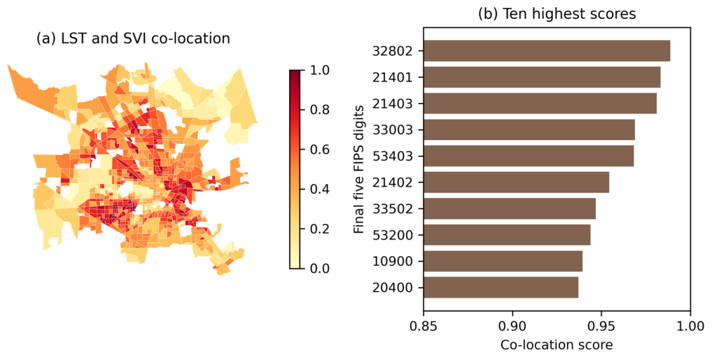
The original three-component score correlated strongly with SVI alone (Spearman ρ = 0.892), while its average health-percentile component also correlated with SVI (ρ = 0.892). The revised two-component score excludes health measures and correlates less strongly with SVI (ρ = 0.739). Original and revised scores remain correlated (ρ = 0.934), with eight shared tracts among their respective top ten. Table 8 and Figure 6 now display the same ten highest revised scores. These rankings describe co-location within the retained sample; neither ranking has demonstrated predictive validity or incremental value for health outcomes.
Table 8.
Ten highest LST–SVI co-location scores in the strict sample. These descriptive ranks are not validated heat-risk priorities.
Figure 6.
Revised LST–SVI co-location score, calculated as the equal-weight mean of the two within-sample percentiles. (a) Spatial distribution. (b) The ten highest scores, labeled by the final five FIPS digits and listed in the same order as Table 8. No health outcome enters the revised score.
5. Discussion
5.1. Primary Findings
The audit identified uncertainty in source-tract assignments, systematic sample exclusions, and associations that varied across model specifications. The source audit reproduced the proportional scaling of health fields and the reported reconstruction counts. It also showed that directly checkable records were less scaled than the remaining records and that exclusions favored warmer, more socially vulnerable tracts. Identifier agreement and near-exact profile similarity therefore cannot be treated as proof of a representative, error-free analytical sample.
The archived source PLACES values agreed with the public release, and the revised outcomes were joined from those source records. This resolves the invalid scaling of the health percentages after source assignment, but it does not independently validate the inferred crosswalk, the weighted temperature values, or the interpolation of SVI ranks. The finding illustrates why technically executable statistical models can produce misleading substantive interpretations when the input geography or measurement scale is wrong.
Age composition partly explains the original conditional pattern. Its inclusion attenuated the stroke coefficient and reduced the lack-of-health-insurance coefficient to near zero in OLS. The obesity and asthma coefficients remained inverse, so age alone did not account for all signs. In contrast, spatial-error modeling reduced all three chronic-disease coefficients toward zero. The data therefore support sensitivity to demographic and spatial specification, not evidence that warmer surfaces protect against chronic disease. The small positive spatial-error association with lack of health insurance remains conditional on the selected model and a single-date temperature field with incomplete archived processing metadata.
The high explained variance after including SVI warrants caution because PLACES estimates already incorporate demographic and socioeconomic information [29,30]. Low global VIFs show that this concern is distinct from strong linear collinearity between LST and SVI. Splitting SVI into themes makes the adjustment more explicit, but does not remove shared model dependence. Likewise, GWR’s improved interpolation and modest local condition numbers do not establish external predictive performance or a mechanism for non-stationarity [35,36]. The spatial-error comparison provides a more restrained assessment of the residual dependence observed in OLS [34].
5.2. Environmental-Justice and Policy Implications
Broader research supports addressing unequal heat exposure and adaptive capacity [13,15,16,17,18], but the present analysis does not establish a validated local heat-health targeting system. Its strongest planning implication concerns the quality of the evidence used for screening: source geography, temperature provenance, modeled outcome dependence, and sample coverage must be documented before rankings guide resource allocation. The revised co-location score removes the health component to reduce redundancy with SVI and avoids assuming that every health indicator has the same temperature relationship.
Shade, vegetation, reflective roofs, accessible cooling, and health outreach remain relevant strategies in the broader literature [11,12,27]. Their location and design should be assessed using verified thermal observations, population exposure, implementation feasibility, and community knowledge. The audited layer and its descriptive rankings can inform questions for further investigation, but cannot establish which intervention or tract would produce the greatest health benefit.
5.3. Limitations
The temperature input is identified as Landsat 8 imagery acquired on 27 September 2022, processed in ArcGIS Pro using the Band 10 and NDVI-based emissivity workflow of Avdan and Jovanovska [38]. The converted LST and NDVI layers and acquisition illustration are now supplied. However, the raw Landsat bands, MTL file, exact calculation expressions, unit-conversion history, pixel-quality mask, and original raster-to-tract log remain unavailable. Supplying the converted output therefore improves data access and workflow documentation without independently reproducing the exact archived LST_MEAN variable or verifying its absolute calibration. The statistical results remain those of the archived-field analysis. A single early-autumn surface-temperature observation cannot quantify peak-summer, nighttime, long-term ambient, or personal heat exposure [9].
Reconstruction also remains uncertain. Although profile agreement, public-source consistency, and centroid containment provide supporting evidence, geographic plausibility is not a complete reference standard for the 642 records without directly comparable identifiers. The validation subset was systematically less affected by scaling, and excluded source tracts differed in temperature, SVI, and health estimates. Similar coefficients across thresholds do not prove that selection bias is absent. Alternative plausible source assignments were not tested; the threshold analyses retain the inferred crosswalk and do not quantify how assignment uncertainty affects the statistical findings. Factor-weighted interpolation of 2020 SVI ranks onto older tracts is an approximation, and the meaning of the inferred scaling factor is not fully documented. The converted temperature raster is now available; a fully documented rebuild still requires confirmation of the original extraction and unit-conversion settings and an explicit geographic crosswalk, beyond direct joins of the public health and social tables.
Finally, the outcomes are crude ecological estimates with shared model inputs and unpropagated uncertainty [29,30]. The directly joined age covariate comes from 2014 to 2018 ACS and does not capture every age-related difference during the PLACES input years. The analysis combines that age measure, 2016–2020 ACS-based SVI, 2020/2019 BRFSS-based PLACES estimates, and a temperature field from the 27 September 2022 Landsat 8 acquisition; these sources represent different observation periods. In particular, the temperature observation follows the 2019/2020 BRFSS inputs and cannot establish an antecedent exposure for those health estimates. Age adjustment, separate SVI themes, and spatial-error modeling improve diagnostic transparency but do not remove omitted-variable bias or establish temporal sequence. GWR bandwidth selection and LOOCV use spatially related observations and the same dataset, while the co-location score remains sensitive to sample coverage and arbitrary equal weighting. These limitations preclude individual-level, causal, clinical, or intervention-effect interpretation.
6. Conclusions
This Houston-area audit identified an apparent multiplicative scaling pattern in health-prevalence fields, recovered 740 source tracts, and evaluated a strict 659-tract sample. Direct source joins restored the focal PLACES values, while comparison of checkable, non-checkable, retained, and excluded records exposed important limits to the original validation and sample coverage.
The substantive associations were weak or sensitive to age and spatial specification. Age adjustment reduced the positive OLS association with lack of health insurance, and spatial-error models provided no conventional statistical evidence for LST associations with the three chronic-disease outcomes. The revised evidence supports a methodological conclusion: compatible geography, correct treatment of prevalence, transparent exclusion checks, and restrained spatial modeling are necessary before interpreting integrated temperature and health data. The single-date, early-autumn Landsat observation, temporal differences among inputs, and ecological study design preclude conclusions about heat-related disease risk. GWR and the revised co-location score remain diagnostic and descriptive analyses, respectively, rather than validated risk or causal analyses.
Supplementary Materials
The following supporting information can be downloaded at: https://www.mdpi.com/article/10.3390/cli14100219/s1. Figure S1. Spatial distribution of retained and excluded reconstructed source tracts. Table S1. Characteristics of directly checkable and non-checkable archived records. Table S2a. Source-tract retention by county. Table S2b. Characteristics of retained and excluded reconstructed source tracts. Table S3a. OLS results with LST as the sole explanatory variable. Table S3b. OLS results with LST and overall reaggregated 2020 SVI. Table S3c. OLS results with LST, overall reaggregated 2020 SVI, and age. Table S3d. OLS results with LST, the four reaggregated 2020 SVI themes, and age. Table S3e. OLS results with LST, native-geography 2018 SVI, and age. Table S4. Standardized LST coefficients under alternative reconstruction thresholds. Table S5a. Spatial-error model results with 4 nearest neighbors. Table S5b. Spatial-error model results with 8 nearest neighbors. Table S5c. Spatial-error model results with 12 nearest neighbors. Table S6a. Candidate GWR bandwidths for lack of health insurance. Table S6b. Candidate GWR bandwidths for obesity. Table S6c. Candidate GWR bandwidths for current asthma. Table S6d. Candidate GWR bandwidths for stroke.
Author Contributions
Conceptualization, G.N., J.Z. and D.R.; methodology, J.Z. and D.R.; formal analysis, J.Z. and D.R.; visualization, D.R.; writing—original draft preparation, D.R.; writing—review and editing, D.R., J.Z. and G.N. All authors have read and agreed to the published version of the manuscript.
Funding
This work was funded by the National Institute of Environmental Health Sciences grant number P30ES029067: Texas A&M Center for Environmental Health Research and the National Institute of Environmental Health Sciences Superfund grant number P42ES027704-01: Comprehensive tools and models for addressing exposure to mixtures during environmental emergency-related contamination events.
Data Availability Statement
Public source data are identified in Table 1 and references [24,30,37]. Houston_Revision_Analysis_Package.zip contains the archived input table, PLACES source values, age-source data, reconstruction crosswalk, reconstructed tract table, existing model and sensitivity outputs, and reproducible analysis scripts. It now also includes the author-supplied Extract_LST_22.lpkx and Extract_NDVI_22.lpkx layer packages, the acquisition illustration, and the Avdan and Jovanovska methods paper [38]. These converted raster layers accompany the 27 September 2022 Landsat 8 and ArcGIS Pro workflow described in Section 3.3. The related Houston publication [28] provides additional context. Raw Landsat bands, original MTL metadata, and complete historical processing and extraction logs are not included. The package retains the existing archived-table analysis; this documentation update does not recalculate its model results. Reproducibility here concerns the analysis of the supplied table, not independent reproduction of the original satellite retrieval or the exact archived LST_MEAN variable.
Conflicts of Interest
The authors declare no conflicts of interest.
Abbreviations
CDC, Centers for Disease Control and Prevention; FIPS, Federal Information Processing Standards; GWR, geographically weighted regression; HC3, heteroskedasticity-consistent covariance estimator type 3; LOOCV, leave-one-out cross-validation; LST, land surface temperature; OLS, ordinary least squares; SVI, Social Vulnerability Index; VIF, variance-inflation factor; ACS, American Community Survey; PRESS, prediction residual sum of squares.
References
- Yang, X.; Xu, X.; Wang, Y.; Yang, J.; Wu, X. Heat exposure impacts on urban health: A meta-analysis. Sci. Total Environ. 2024, 947, 174650. [Google Scholar] [CrossRef] [Scilit]
- Tuholske, C.; Caylor, K.; Funk, C.; Verdin, A.; Sweeney, S.; Grace, K.; Peterson, P.; Evans, T. Global urban population exposure to extreme heat. Proc. Natl. Acad. Sci. USA 2021, 118, e2024792118. [Google Scholar] [CrossRef] [Scilit]
- Vicedo-Cabrera, A.M.; Scovronick, N.; Sera, F.; Royé, D.; Schneider, R.; Tobias, A.; Åström, C.; Guo, Y.; Honda, Y.; Hondula, D.M.; et al. The burden of heat-related mortality attributable to recent human-induced climate change. Nat. Clim. Chang. 2021, 11, 492–500. [Google Scholar] [CrossRef] [Scilit]
- Heaviside, C.; Macintyre, H.; Vardoulakis, S. The urban heat island: Implications for health in a changing environment. Curr. Environ. Health Rep. 2017, 4, 296–305. [Google Scholar] [CrossRef] [Scilit]
- Piracha, A.; Chaudhary, M.T. Urban air pollution, urban heat island and human health: A review of the literature. Sustainability 2022, 14, 9234. [Google Scholar] [CrossRef] [Scilit]
- Ellena, M.; Breil, M.; Soriani, S. The heat-health nexus in the urban context: A systematic literature review exploring the socio-economic vulnerabilities and built-environment characteristics. Urban Clim. 2020, 34, 100676. [Google Scholar] [CrossRef] [Scilit]
- Cleland, S.E.; Steinhardt, W.; Neas, L.M.; West, J.J.; Rappold, A.G. Urban heat island impacts on heat-related cardiovascular morbidity: A time-series analysis of older adults in U.S. metropolitan areas. Environ. Int. 2023, 178, 108005. [Google Scholar] [CrossRef] [Scilit]
- U.S. Geological Survey. Landsat Collection 2 Surface Temperature. Available online: https://www.usgs.gov/landsat-missions/landsat-collection-2-surface-temperature (accessed on 16 August 2025).
- Venter, Z.S.; Chakraborty, T.; Lee, X. Crowdsourced air temperatures contrast satellite measures of the urban heat island and its mechanisms. Sci. Adv. 2021, 7, eabb9569. [Google Scholar] [CrossRef] [Scilit]
- Hulley, G.; Shivers, S.; Wetherley, E.; Cudd, R. New ECOSTRESS and MODIS land surface temperature data reveal fine-scale heat vulnerability in cities: A case study for Los Angeles County, California. Remote Sens. 2019, 11, 2136. [Google Scholar] [CrossRef] [Scilit]
- Murage, P.; Hajat, S.; Macintyre, H.L.; Leonardi, G.S.; Ratwatte, P.; Wehling, H.; Petrou, G.; Higlett, M.; Hands, A.; Kovats, S. Indicators to support local public health to reduce the impacts of heat on health. Environ. Int. 2024, 183, 108391. [Google Scholar] [CrossRef] [Scilit]
- Jay, O.; Capon, A.; Berry, P.; Broderick, C.; de Dear, R.; Havenith, G.; Honda, Y.; Kovats, R.S.; Ma, W.; Malik, A.; et al. Reducing the health effects of hot weather and heat extremes: From personal cooling strategies to green cities. Lancet 2021, 398, 709–724. [Google Scholar] [CrossRef] [Scilit]
- Slesinski, S.C.; Matthies-Wiesler, F.; Breitner-Busch, S.; Gussmann, G.; Schneider, A. Social inequalities in exposure to heat stress and related adaptive capacity: A systematic review. Environ. Res. Lett. 2025, 20, 033005. [Google Scholar] [CrossRef] [Scilit]
- Gronlund, C.J. Racial and socioeconomic disparities in heat-related health effects and their mechanisms: A review. Curr. Epidemiol. Rep. 2014, 1, 165–173. [Google Scholar] [CrossRef] [Scilit]
- Hsu, A.; Sheriff, G.; Chakraborty, T.; Manya, D. Disproportionate exposure to urban heat island intensity across major U.S. cities. Nat. Commun. 2021, 12, 2721. [Google Scholar] [CrossRef] [Scilit]
- Johnson, D.P. Population-based disparities in U.S. urban heat exposure from 2003 to 2018. Int. J. Environ. Res. Public Health 2022, 19, 12314. [Google Scholar] [CrossRef] [Scilit]
- Chakraborty, T.; Hsu, A.; Manya, D.; Sheriff, G. Disproportionately higher exposure to urban heat in lower-income neighborhoods: A multi-city perspective. Environ. Res. Lett. 2019, 14, 105003. [Google Scholar] [CrossRef] [Scilit]
- Hoffman, J.S.; Shandas, V.; Pendleton, N. The effects of historical housing policies on resident exposure to intra-urban heat: A study of 108 U.S. urban areas. Climate 2020, 8, 12. [Google Scholar] [CrossRef] [Scilit]
- Li, F.; Yigitcanlar, T.; Nepal, M.; Thanh, K.; Dur, F. Understanding urban heat vulnerability assessment methods: A PRISMA review. Energies 2022, 15, 6998. [Google Scholar] [CrossRef] [Scilit]
- Fall, S.; Coulibaly, K.; Quansah, J.; El Afandi, G. Differential urban heat vulnerability: The tale of three Alabama cities. Urban Sci. 2023, 7, 121. [Google Scholar] [CrossRef] [Scilit]
- Cresswell, K.; Mitsova, D.; Liu, W.; Fadiman, M.; Hindle, T. Gauging heat vulnerability in Southeast Florida: A multimodal approach integrating physical exposure, sensitivity, and adaptive capacity. ISPRS Int. J. Geo-Inf. 2023, 12, 242. [Google Scholar] [CrossRef] [Scilit]
- Li, F.; Yigitcanlar, T.; Nepal, M.; Thanh, K.N.; Dur, F. A novel urban heat vulnerability analysis: Integrating machine learning and remote sensing for enhanced insights. Remote Sens. 2024, 16, 3032. [Google Scholar] [CrossRef] [Scilit]
- Niu, Y.; Li, Z.; Gao, Y.; Liu, X.; Xu, L.; Vardoulakis, S.; Yue, Y.; Wang, J.; Liu, Q. A systematic review of the development and validation of the heat vulnerability index: Major factors, methods, and spatial units. Curr. Clim. Change Rep. 2021, 7, 87–97. [Google Scholar] [CrossRef] [Scilit]
- Centers for Disease Control and Prevention; Agency for Toxic Substances and Disease Registry. CDC/ATSDR Social Vulnerability Index 2020 Data and Documentation. Available online: https://www.atsdr.cdc.gov/place-health/php/svi/svi-data-documentation-download.html (accessed on 15 September 2026).
- National Weather Service Houston/Galveston. Houston IAH Climate Normals and Summaries. Available online: https://www.weather.gov/hgx/climate_iah_normals_summary (accessed on 15 September 2026).
- Nowak, D.J.; Bodine, A.R.; Hoehn, R.E., III; Edgar, C.B.; Riley, G.; Hartel, D.R.; Dooley, K.J.; Stanton, S.M.; Hatfield, M.A.; Brandeis, T.J.; et al. Houston’s Urban Forest, 2015; Resource Bulletin SRS-211; U.S. Department of Agriculture, Forest Service, Southern Research Station: Asheville, NC, USA, 2017; 91p. [CrossRef] [Scilit]
- Fung, K.Y.; Yang, Z.-L.; Martilli, A.; Krayenhoff, E.S.; Niyogi, D. Prioritizing social vulnerability in urban heat mitigation. PNAS Nexus 2024, 3, pgae360. [Google Scholar] [CrossRef] [Scilit]
- Ren, D.; Newman, G.; Brown, R.D.; Li, D.; Zou, L. Determining the impact of urban vacant and abandoned land on land surface temperatures in socially vulnerable communities in Houston. Climate 2026, 14, 78. [Google Scholar] [CrossRef] [Scilit]
- Greenlund, K.J.; Lu, H.; Wang, Y.; Matthews, K.A.; LeClercq, J.M.; Lee, B.; Carlson, S.A. PLACES: Local data for better health. Prev. Chronic Dis. 2022, 19, E31. [Google Scholar] [CrossRef] [Scilit]
- Centers for Disease Control and Prevention. PLACES Census Tract Data GIS Friendly Format 2022 Release [Dataset]. Available online: https://catalog.data.gov/dataset/places-census-tract-data-gis-friendly-format-2022-release (accessed on 15 September 2026).
- Lucas, K.; DeWitt, B.; Biddle, D.J.; Zhang, C.H. A spatial analysis of the association between urban heat and coronary heart disease. ISPRS Int. J. Geo-Inf. 2025, 14, 344. [Google Scholar] [CrossRef] [Scilit]
- Gasparrini, A.; Guo, Y.; Hashizume, M.; Lavigne, E.; Zanobetti, A.; Schwartz, J.; Tobias, A.; Tong, S.; Rocklöv, J.; Forsberg, B.; et al. Mortality risk attributable to high and low ambient temperature: A multicountry observational study. Lancet 2015, 386, 369–375. [Google Scholar] [CrossRef] [Scilit]
- Moran, P.A.P. The interpretation of statistical maps. J. R. Stat. Soc. Ser. B 1948, 10, 243–251. [Google Scholar] [CrossRef] [Scilit]
- Anselin, L. Spatial Econometrics: Methods and Models; Kluwer Academic Publishers: Dordrecht, The Netherlands, 1988. [Google Scholar] [CrossRef] [Scilit]
- Comber, A.; Brunsdon, C.; Charlton, M.; Dong, G.; Harris, R.; Lu, B.; Lü, Y.; Murakami, D.; Nakaya, T.; Wang, Y.; et al. A route map for successful applications of geographically weighted regression. Geogr. Anal. 2023, 55, 155–178. [Google Scholar] [CrossRef] [Scilit]
- Kiani, B.; Sartorius, B.; Lau, C.L.; Bergquist, R. Mastering geographically weighted regression: Key considerations for building a robust model. Geospat. Health 2024, 19, 1271. [Google Scholar] [CrossRef] [Scilit]
- Centers for Disease Control and Prevention; Agency for Toxic Substances and Disease Registry. CDC SVI 2018 Documentation, Updated 19 January 2022; 2014–2018 American Community Survey Estimates. Available online: https://svi.cdc.gov/map25/data/docs/SVI2018Documentation_01192022_1.pdf (accessed on 15 September 2026).
- Avdan, U.; Jovanovska, G. Algorithm for automated mapping of land surface temperature using LANDSAT 8 satellite data. J. Sens. 2016, 2016, 1480307. [Google Scholar] [CrossRef] [Scilit]

Disclaimer/Publisher’s Note: The statements, opinions and data contained in all publications are solely those of the individual author(s) and contributor(s) and not of MDPI and/or the editor(s). MDPI and/or the editor(s) disclaim responsibility for any injury to people or property resulting from any ideas, methods, instructions or products referred to in the content. |
© 2026 by the authors. Licensee MDPI, Basel, Switzerland. This article is an open access article distributed under the terms and conditions of the Creative Commons Attribution (CC BY) license.