


Abstract
Urban expansion is often tracked with annual land-cover data, yet year-to-year classification noise can masquerade as persistent urban growth. Previous work has usually treated detection, morphology, spatial structure, driver analysis, and forward-looking modelling separately. Here we follow urban growth in Tehran County from 2016 to 2025 within one linked workflow and then extend the analysis to a 2025–2030 growth-pressure screening under static covariates. Annual 10 m built-up composites from Dynamic World were passed through a temporal stability filter to retain persistent change. Stable growth was classified into four regimes, tested for clustering and interaction scale, and examined using a Spatial Durbin Model and multiscale geographically weighted regression. A two-stage machine-learning branch then produced a ranked growth-pressure surface. In this study, growth-pressure screening means identifying where recent spatial conditions are most compatible with continued growth under unchanged covariates; it is intended for relative spatial ranking under stated assumptions rather than deterministic estimation of future urbanization. Stable new built-up area totaled 107.64 km2, most of it ribbon growth (57.60%) and edge expansion (32.77%). A stratified local validation of 300 samples returned a weighted overall accuracy of 97.30%, and a 27-scenario threshold test retained ribbon growth as the largest regime and edge expansion as the second largest in every case. Clustering was significant (Global Moran’s I = 0.326), with a dominant interaction range of about 8–10 km. Historical backtesting showed strong discrimination and ranking (ROC AUC = 0.979; PR AUC = 0.984; Spearman ρ = 0.902), while exact growth-magnitude performance was more moderate (R2 = 0.341). The growth-pressure surface is therefore more useful for hotspot identification and relative ranking than for estimating exact future growth magnitude.
1. Introduction
Urban growth poses a major challenge for metropolitan areas where expansion is rapid, uneven, and difficult to manage. As built-up land extends into agricultural and open areas, urban growth increases infrastructure demand, intensifies pressure on land, and places additional burdens on planning systems [1]. It therefore needs to be examined not only through the amount of land added, but also through the location, form, and spatial processes of expansion. Tehran County provides a relevant case because the wider metropolitan area has experienced long-term outward growth, peripheral development, and continuing concerns about sprawl and spatial restructuring [2,3].
Annual built-up mapping and remote-sensing-based change detection remain an important basis for understanding recent urban expansion, as they allow land conversion to be tracked across large metropolitan areas with a level of spatial consistency rarely provided by traditional records [4,5,6]. Annual land-cover outputs, however, do not necessarily produce stable urban trajectories. Year-specific maps can contain scene-to-scene variation, compositing effects, classification uncertainty, and short-lived switching between built and non-built labels, especially in cities with heterogeneous building forms [7,8]. Consequently, the annual record may not always reflect actual urban change. Some apparent gains or losses may result from instability in the mapped signal rather than longer-term change in the urban fabric. Separating persistent growth from short-term fluctuation therefore provides a more stable basis for interpretation. Temporal persistence alone, however, does not explain the spatial form taken by expansion once it becomes established.
The spatial pattern of urban growth is important because cities do not grow evenly. The pattern of new construction often provides important information about land use and the distribution of pressure across the broader urban area [9,10,11]. Research on sprawl and densification has demonstrated that distinguishing between different types of growth is not a purely descriptive exercise, as infill, corridor-oriented development, and outward expansion have different planning implications and consequences for land efficiency and fragmentation [12,13,14]. Recent urban expansion can thus be classified into four main regimes: infill, ribbon, edge expansion, and leapfrog, which help to differentiate between development within the existing urban fabric, along transportation corridors, on the urban fringe, or in more isolated peripheral areas [15,16,17].
This distinction is also relevant in Tehran, where earlier and more recent work points to outward growth, heterogeneous urban form, and continuing change across the metropolitan edge rather than simple internal consolidation alone [18,19,20]. Even so, morphology by itself is still not enough, because identifying the visible form of expansion does not yet show whether those forms are clustered, dispersed, or organized at broader metropolitan scales. That wider spatial organization matters in its own right, and it leads directly to the next question of how the main drivers of urban growth operate across space and scale.
Once the main growth patterns and their broader spatial organization have been identified, the next question is what factors are associated with them and whether those relationships remain stable across the metropolitan region or vary from one part of the city to another [21,22]. This question has become increasingly relevant as urban planning relies more heavily on spatial data [23,24]. The value of large urban datasets depends not only on their availability, but also on whether they can support interpretation, coordination, and decision making [25,26,27]. Some influences may operate through broader metropolitan dependence and spatial spillovers that extend beyond the location under examination [21,28,29]. Others may vary locally in strength, direction, and effective spatial scale. A combined global spatial-econometric and local multiscale perspective is therefore analytically useful [22,30,31]. A separate growth-pressure screening branch can then identify areas where recent conditions may persist under stated assumptions, without treating the surface as a deterministic representation of Tehran’s future [32,33,34]. The SDM and MGWR are used for different purposes: the SDM examines broad spatial dependence and spillover effects, whereas MGWR shows how the same relationships vary locally and at different spatial scales. The final screening branch is separate from both and is used only to rank where recent growth pressure may continue if the covariates remain unchanged.
Research on urban expansion has established methods for annual change detection, urban morphology, spatial-structure analysis, and forward-looking applications [31,35,36,37,38,39,40], but these components are often applied separately. Studies that connect persistence-filtered expansion, regime classification, scale detection, global–local driver analysis, and conditional growth-pressure screening within one question-led sequence remain uncommon [31,35,37]. This study addresses that gap for Tehran County during 2016–2025 and extends the framework to a cautious 2025–2030 screening. Its contribution is therefore integrative rather than the introduction of a new method.
Accordingly, this study addresses the following research questions:
- What does a persistence-based analysis reveal about recent stable urban expansion in Tehran County beyond the annual built-up record during 2016–2025?
- Which growth regimes dominate recent stable urban expansion in Tehran County, and how are they distributed across the metropolitan landscape?
- What spatial structure and dominant interaction scale characterize recent urban growth in Tehran County, and how robust are these patterns to alternative neighborhood definitions and changes in analytical aggregation?
- Which factors are associated with recent urban growth in Tehran County at global and local scales, how do the SDM and MGWR complement each other, and how can the resulting relationships support growth-pressure screening for 2025–2030?
2. Literature Review
2.1. Urban Growth Mapping, Stable Expansion, and Growth Morphology
A change observed in a single annual map does not necessarily represent a permanent change in urban land. Annual or subannual land-cover products reduce a gradual and sometimes reversible process to a sequence of discrete labels. Urbanization may proceed unevenly, with interruptions, reversals, and spatial variation. Wang et al. make a related argument at a broader scale, noting that commonly used urban growth metrics often represent particular temporal snapshots and may omit parts of the longer development trajectory [41]. Other studies similarly show that coarse temporal sampling can obscure transient changes and rapid transitions, particularly in fast-changing urban environments [42]. The issue is therefore both technical and interpretive. Shafizadeh-Moghadam et al. found that the influence of growth drivers in the Tehran-Karaj area varied across time intervals, indicating that recent expansion should not be treated as temporally fixed or spatially uniform [43]. This literature suggests that annual mapping is best used as an analytical starting point and that longer-term growth should be separated from short-term or unstable change signals [41,42,43].
Recent typological research on urban sprawl and urban fabric has examined distinctions among infill, near-edge extension, detached outward development, and other spatial forms, while emphasizing that no single metric captures this complexity [44,45]. Regime-based classification provides one way to organize these differences. These categories are not defined in exactly the same way across studies, and their numerical cutoffs often depend on spatial resolution, urban form, the way roads and urban edges are represented, and the purpose of the analysis [44,45]. Thresholds used in one city should therefore not be treated as universal values; they need to be stated clearly and tested for sensitivity. Infill, edge expansion, ribbon or corridor development, and leapfrog growth distinguish compactification from peripheral spread, accessibility-related growth from detached patch formation, and continuous urbanization from fragmented outward expansion. Research on leapfrogging further shows that scattered outward growth represents an observable process rather than only a visual pattern [46]. Studies of the Tehran-Karaj region indicate that expansion is spatially uneven, temporally sensitive, and increasingly connected across adjacent urban areas rather than reducible to one general trend [43]. A robust assessment therefore requires both the detection of change and the identification of the specific growth forms present before their spatial organization and possible drivers are examined.
2.2. Urban Growth: Spatial Structure, Clustering and Scale
Once the main growth forms are identified, the next task is to determine how they are organized spatially. Urban expansion is typically uneven, with some areas experiencing concentrated change and others remaining stable or changing in a more fragmented manner. Research has therefore moved beyond area totals toward spatial autocorrelation, local cluster detection, and hotspot analysis [47,48]. Moran’s I and Local Indicators of Spatial Association (LISA), among other tools, can show whether growth is clustered, dispersed, or locally variable. Combining urban-growth mapping with exploratory spatial data analysis has shown that metropolitan expansion often follows structured core-periphery patterns rather than a random distribution. Studies in Iran have similarly reported positive spatial autocorrelation in urbanization, particularly around Tehran [49,50].
Spatial scale adds a further source of complexity. A pattern may appear strongly clustered at one analytical resolution but weaker or differently organized at another, making the observed spatial structure inseparable from the scale of measurement. Scale-sensitive analysis has therefore become increasingly important in urban growth research, particularly when the objective is to identify the spatial extent at which a pattern is most evident [51,52,53]. Studies of multiscale urban expansion show that both delineation and interpretation can change with the observational window or analytical unit [54,55]. Once growth form has been identified, analysis should therefore move from visible morphology to spatial organization before proceeding to explanation.
2.3. Global and Local Modeling of Urban-Growth Drivers and Forward-Looking Approaches
Research on urban-growth drivers has gradually moved away from models that treat urban change as a purely local process. A growing part of the literature now starts from a simpler but more realistic assumption: growth in one place is often shaped by what is happening nearby, and the same driver may not work in the same way across the whole urban region. This has led to two closely related directions in the field. One relies on global spatial models to estimate broad relationships and spillover effects. The other takes a local view and asks whether those relationships become stronger, weaker, or even different in sign from one place to another. In the Tehran metropolitan region, Alaei Moghadam et al. show why this matters by modeling growth as a process shaped by spatial interactions between cities rather than as isolated local change [56]. Similar conclusions emerge from studies that compare spatial econometric models or use geographically weighted approaches to examine drivers of urban expansion, showing that both broader spatial dependence and local variation matter for explanation [57,58].
A smaller but important part of the literature extends this line of work into forward-looking analysis. In most cases, the purpose is not to predict an exact urban future, but to examine how growth or land consumption may develop under particular assumptions, planning priorities, or demand conditions. Rienow et al. follow this logic by exploring how regional planning and climate-related strategies could reshape future land consumption in the Rhine–Ruhr metropolitan area [59]. A similar planning-oriented perspective appears in Lee and Lee, who connect land-use change modelling with future land-demand scenarios in Seoul [60]. Forward-looking modelling is most useful when it builds on spatial explanation rather than replacing it. Even so, global inference, local modelling, and prospective analysis are still often presented separately, leaving the wider analytical sequence only partly connected.
2.4. Research Gaps
The literature provides mature approaches for mapping urban change, classifying growth form, identifying spatial structure and scale, modelling global and local relationships, and examining planning-oriented futures [41,43,44,49,54,56,59,60]. These components, however, are less often connected within one analytical sequence. The present study addresses this methodological gap by linking temporal persistence, growth morphology, spatial scale, driver analysis, and conditional screening while keeping their analytical roles distinct. A second gap is contextual: studies of Tehran often identify where growth occurs but less often relate the observed pattern to municipal finance, land-management institutions, density regulation, and access to formal housing [61,62,63,64,65]. These institutional factors are not modelled as causal predictors here but provide an important context for interpreting the mapped pattern.
3. Materials and Methods
3.1. Study Area and Analytical Design
Tehran County was selected as the study area because it is part of a metropolitan region that has undergone continuous outward expansion, major land-use change, and noticeable spatial reorganization over recent decades. Earlier studies have shown that urban growth in this area has been rapid but uneven, with strong development pressure along the metropolitan fringe and ongoing concern about urban sprawl and the extension of city boundaries. These characteristics make Tehran an appropriate case for examining recent built-up growth not only in terms of extent but also in terms of growth morphology, spatial clustering, and local variation in urban growth drivers [2,3].
The analysis was carried out within the political boundary of Tehran County, which was treated as the single authoritative study extent throughout all processing stages. All spatial layers were prepared in UTM Zone 39N (EPSG:32639). Raster-based change detection and land-cover processing were conducted at 10 m spatial resolution, whereas spatial statistical analysis and modelling were implemented on a fixed 500 × 500 m analytical grid. The historical component covers 2016–2025, and a separate growth-pressure screening branch was developed for 2025–2030. Tehran City refers to the municipality-centered urban core, whereas Tehran County is the larger administrative unit used as the analytical extent; the two boundaries are not identical. Figure 1 has been relabeled accordingly to remove the earlier ambiguity.
Figure 1.
Location of Tehran County within Tehran Province and Iran. The red outline denotes Tehran County, which is the analytical study area.
3.2. Data Sources
The analysis drew on a combination of remotely sensed, topographic, infrastructural, demographic, and study-derived spatial data. Dynamic World V1 provided the annual land-cover basis for mapping built-up change, while the Tehran County boundary defined the common spatial extent of the analysis. OpenStreetMap major roads were used to represent road-network proximity, NASADEM supported the extraction of elevation and slope, and WorldPop 2016 was used to characterize population density. Additional derived layers from earlier processing stages were then carried forward to the later spatial analyses and modeling steps. The input datasets and their analytical roles are summarized in Table 1.
Table 1.
Input datasets and their role in the analytical framework.
Taken together, these datasets provided the land cover, road network, terrain, population, and derived spatial information required for the subsequent analysis of urban growth patterns and drivers.
3.3. Overall Analytical Workflow
The workflow was organized in four linked stages. In the first stage, annual land-cover layers were generated from Dynamic World V1 to establish the built-up change baseline for 2016–2025. In the second stage, stable new built-up areas were identified, urban expansion was classified into distinct growth regimes, and the main explanatory variables were aggregated to the 500 m analytical grid. The third stage focused on spatial autocorrelation and scale detection, with the aim of identifying the dominant interaction distance and defining a common spatial-weights matrix for the subsequent analysis. In the final stage, global and local growth drivers were examined using spatial econometric and multiscale geographically weighted approaches, after which the workflow was extended to a growth-pressure screening branch for 2025–2030. The stages were linked because they answer different questions, not because they repeat the same analysis with several tools.
Figure 2 summarizes the analytical sequence and the distinct role of each phase: Phase 1 establishes the annual built-up baseline; Phase 2 isolates persistent expansion and its morphology; Phase 3 identifies spatial clustering and interaction scale; and Phase 4 interprets global and local drivers and produces the conditional growth-pressure screening surface.
Figure 2.
Four-phase analytical workflow and the analytical role of each stage.
3.4. Annual Built-Up Mapping, Growth-Regime Classification, and Variable Preparation
The annual built-up baseline was derived from Dynamic World V1, which provides near-real-time 10 m land-cover predictions from Sentinel-2 imagery rather than preassembled annual maps. Because Dynamic World outputs are generated at the image level and the collection is updated continuously, annual summaries aggregate many scene-level predictions acquired under different observation conditions. This temporal detail is useful for recent change monitoring, but short-term classification variability can also propagate into yearly built-up estimates. Brown et al. reported strong built-area performance in the product’s global validation, with 86.7% user accuracy and 88.4% producer accuracy under expert-consensus labeling [4], while Venter et al. found 72% overall accuracy in a global comparison and identified built area as one of the better-mapped classes [7]. Independent comparisons have also shown that the suitability of recent 10 m global land-cover products depends on application context and study area [8]. Recent work in semi-arid heritage cities has likewise combined Dynamic World with independent high-resolution-image validation, underlining the need for local checks in dry urban environments [66]. Published accuracies were therefore treated as background evidence rather than as a substitute for local assessment. A Tehran-specific validation of the stable-expansion layer was carried out as described below, while the annual series was still interpreted cautiously because local validation cannot remove all annual classification variability.
For that reason, the annual series was treated as an initial built-up baseline rather than as the sole evidential basis for interpreting recent urban expansion. To reduce seasonal noise and improve year-to-year comparability, only observations acquired between 1 April and 31 October were retained for each year, annual land-cover maps were produced as mode composites, and a minimum of five valid observations per pixel per year was required before compositing. For change analysis, the annual outputs were simplified into three binary classes, built-up, vegetation, and bare land, and a 3 × 3 morphological opening filter was applied to each class mask to remove isolated speckle and very small artefacts. Subsequent change detection therefore did not rely on single-year transitions alone. Instead, the main expansion layer was derived from a temporal stability rule that retained only pixels not built-up in 2016 but classified as built-up in at least two of the three final years, thereby reducing the influence of short-lived annual misclassification.
All outputs from this step were exported at 10 m spatial resolution in UTM Zone 39N (EPSG:32639) and carried forward as baseline inputs for the later stages of the study.
The analysis then turned to identifying persistent urban expansion and describing its spatial form.
where is a binary indicator equal to 1 if pixel is classified as built-up in year , and 0 otherwise. Because the annual built-up series may still contain short-lived class switching, the interpretation of recent expansion was based on persistence rather than one-year transitions alone. Accordingly, was defined as 1 for pixels that were not built-up in 2016, that is, , but were classified as built-up in at least two of the three final years, meaning that . This rule was introduced to suppress transient classification noise near the end of the study period and to retain only those changes that persisted across multiple closing years. In this way, the annual series was used to map possible change trajectories, whereas the stable-expansion layer served as the main evidential basis for interpreting recent urban growth. The 2-of-3 rule was chosen as a middle position: it required the built-up signal to appear in more than one closing year, but it did not discard a change simply because one annual composite differed. This was treated as an operational choice rather than a universal definition, and its influence was tested using alternative persistence rules.
To assess the stable-expansion layer locally, a probability-based stratified sample was drawn from a validation area covering Tehran’s urban boundary and a 5 km surrounding buffer, restricted to pixels that were valid in both the 2016 baseline and stable-expansion rasters. The primary sample contained 300 source-raster pixels at the native 10 m resolution: 150 mapped as stable expansion, 60 mapped as pre-existing built-up land, and 90 drawn from the remaining non-expansion area. A 15% reserve sample was also selected within each stratum before interpretation.
Each primary sample was assessed using multi-temporal satellite imagery available in Google Earth Pro (version 7.3.7) for 2016, 2023, and 2025 so that persistent construction could be distinguished from pre-existing built-up land, stable non-built land, temporary disturbance, loss or demolition, and uncertain cases. All 300 sample locations were visually assessed by the researcher. The binary reference labels were combined with the mapped area weight of each stratum to estimate a design-weighted error matrix, overall and class-specific accuracy measures, and an error-adjusted expansion area. Uncertainty was estimated from 5000 bootstrap repetitions using 95% confidence intervals. The sample records and full accuracy assessment are provided in Tables S1 and S2.
Persistence sensitivity was examined while keeping the 2016 non-built baseline and all later regime-classification rules unchanged. The closing-period test included 1-of-3, 2-of-3, and 3-of-3 rules for 2023–2025, together with 3-of-5, 4-of-5, and 5-of-5 rules for 2021–2025. For each rule, the stable-expansion area, overlap with the primary 2-of-3 map, and the area share and ranking of the four growth regimes were recalculated. The full comparison is reported in Table S4. The growth-regime decision rules used in the classification are summarized in Table 2.
Table 2.
Growth-regime decision rules.
The stable new built-up pixels were then classified into four hierarchical growth regimes. This classification was designed to identify spatially meaningful forms of recent expansion that are often discussed in the urban-growth literature, namely infill, edge expansion, leapfrog growth, and corridor-oriented or ribbon development [16,67]. These four types were retained because they represent contrasting ways in which urban growth is expressed spatially and therefore provide a useful basis for the later spatial analyses. Ribbon growth was retained as a separate regime since road-oriented expansion would otherwise be absorbed into the broader edge or leapfrog classes. These classes were not defined using universal numerical thresholds. Rather, they are presented here as study-specific operational rules to construct a mutually exclusive and internally consistent classification framework for Tehran. The 10 ha threshold was used to limit infill to relatively small enclosed voids within the 2016 urban fabric rather than larger interior open areas. The 200 m threshold was used to identify growth that remained closely associated with major roads, while the 300 m threshold was used to capture growth that remained close to the 2016 urban edge at the 10 m analysis resolution used here. In this way, the three cutoffs were used to separate enclosed filling, road-oriented expansion, and near-edge growth within one consistent classification scheme. Within this framework, infill was defined as stable new built-up pixels within enclosed holes in the 2016 urban fabric, with the size of the hole limited to 10 ha under 8-neighbor connectivity. Ribbon growth was defined as stable new built-up pixels within 200 m of major roads, here defined as OSM motorway, trunk, primary, and secondary roads. Edge expansion was defined as stable new built-up pixels within 300 m of the 2016 urban edge after infill and ribbon pixels had been assigned. Any stable new built-up pixel that was not classified as infill, ribbon, or edge was classified as leapfrog growth. If a pixel met more than one rule, assignment was based on the classification hierarchy: infill was prioritized over ribbon, ribbon over edge expansion, and leapfrog was reserved for the remaining stable new built-up pixels.
Because the three cutoffs are operational rather than universal, their influence was examined through a full-factorial sensitivity analysis. Infill-hole thresholds of 7.5, 10, and 12.5 ha, road-distance thresholds of 150, 200, and 250 m, and edge-distance thresholds of 225, 300, and 375 m were combined to produce 27 scenarios. The classification hierarchy was held unchanged in every run. Each scenario was compared with the primary 10 ha, 200 m, and 300 m classification using pixel-level agreement, regime shares and rankings, and class-specific spatial overlap. The primary setting was first required to reproduce the published regime map exactly. Detailed results for all combinations are provided in Table S3.
The final part of this stage prepared the variables needed for the spatial analyses that followed. The built-up baseline, the distance-to-edge and distance-to-roads rasters, and the main environmental and demographic covariates were aggregated onto a fixed 500 × 500 m grid, giving a single analytical base for the subsequent statistical and model-based stages. Area- and count-based variables were summarized as cell totals, continuous variables as cell means, and the dominant growth regime in each cell was assigned as the modal class. Cells with insufficient spatial coverage were excluded so that the later analyses rested on a consistent grid-based representation of urban growth, accessibility, topographic constraints, and socio-spatial pressure across the study area. The 500 × 500 m resolution was chosen as a practical compromise, fine enough to preserve local variation within Tehran County and coarse enough to support stable spatial-statistical and model-based estimation. The 10 m grid was retained only for the land-cover change and distance-based morphology steps, where immediate aggregation to 500 m would have removed narrow road-related and edge features. The 30 m NASADEM and 100 m WorldPop inputs were not interpreted as gaining new 10 m detail; they were aligned for spatial overlay and then summarized to the 500 m modelling cells. Continuous variables were represented by cell means, while area, count, and categorical outputs were summarized by totals or modal classes. The 500 m grid, rather than an artificially sharpened 10 m surface, was therefore the actual spatial support of the SDM, MGWR, and XGBoost analyses.
3.5. Spatial Structure and Scale Detection
The spatial structure of urban growth was examined in three linked stages. First, Global Moran’s I was calculated for total built-up gain to determine whether the observed pattern was spatially clustered rather than random. The test used a fixed-distance specification of 1000 m and 9999 permutations. This initial distance served only as an exploratory setting for confirming significant positive spatial autocorrelation before the multiscale analysis.
where is the number of spatial units, and are the observed values at locations and , is the mean of the variable, is the spatial weight between units and , and .
After confirming significant spatial clustering, the next stage identified the characteristic interaction scale of urban growth. Incremental spatial autocorrelation was applied across 30 fixed distance bands from 500 m to 15,000 m at 500 m intervals. The procedure was conducted for total built-up gain and for the principal regime components retained for spatial interpretation, namely edge-expansion gain and leapfrog gain. For each distance band, a standardized Moran’s I z-score was calculated, and the distance with the strongest clustering signal was interpreted as the peak interaction distance. For total built-up gain, this peak occurred at 8500 m. The 8.5 km value was retained as the operational bandwidth for the main weights matrix, while the later sensitivity and MAUP tests were used to determine whether it should be interpreted more broadly.
Based on this result, local spatial structure was investigated using a common row-standardized fixed-distance weights matrix derived from . Univariate Local Indicators of Spatial Association (LISA) were computed for total built-up gain, edge-expansion gain, and leapfrog gain in order to identify local clusters and spatial outliers. In addition, bivariate LISA was applied to assess the spatial association between total built-up gain and distance to the central business district, while Getis–Ord statistics were used to detect local hot spots and cold spots of total growth intensity. All local statistics were estimated using 9999 permutations.
Because these local procedures involve multiple simultaneous significance tests, false discovery rate (FDR) correction was applied before interpretation. Only FDR-significant local clusters and hotspot patterns were retained in the final analytical outputs. This step was adopted to reduce the risk of spurious local significance and to provide a more conservative interpretation of the spatial structure of growth.
The robustness of the detected spatial pattern was evaluated in two ways. First, bandwidth sensitivity was assessed by repeating the univariate LISA analysis for total built-up gain at moderately smaller and larger distances, with agreement against the baseline quantified using Cohen’s kappa. Second, sensitivity to the modifiable areal unit problem (MAUP) was examined by repeating scale detection on an aligned 1000 m grid derived from the original 500 m framework. The bandwidth test showed high agreement with the baseline solution. The MAUP test, however, shifted the peak interaction distance from 8500 m to 9500 m. Accordingly, 8.5 km is reported as the operational distance used in the core analysis, whereas approximately 8–10 km is used as the more conservative interpretation of the dominant interaction range.
3.6. Spatial Modelling, Local Multiscale Analysis, and Growth-Pressure Screening
The first branch was inferential and examined the spatial factors associated with observed urban expansion. The second was a growth-pressure screening branch that estimated the relative location and intensity of potential future growth under a static-covariate scenario. Both branches used the same 500 × 500 m analytical grid but were estimated independently. The inferential analysis used the master spatial-weights matrix established in the preceding stage, whereas the screening analysis was implemented separately within a machine-learning framework.
Table 3 summarizes the explanatory variables used in the inferential and screening analyses. Together, they represent metropolitan centrality, road accessibility, proximity to the established urban edge, baseline urban intensity, topographic constraints, and demographic pressure. Elevation and slope were both included as topographic variables because they represent different aspects of terrain. All predictors were aggregated from their original resolution to the 500 × 500 m analytical grid and standardized before estimation. Standardization places the predictors on a common variance scale and supports comparison within the same model, but coefficient magnitude should not be interpreted as a direct measure of causal importance.
Table 3.
Explanatory variables used in the inferential and growth-pressure screening analyses.
The seven explanatory variables in Table 3 were selected to cover the main driver categories commonly used in urban growth modelling: accessibility, proximity to existing urban fabric, prior urbanization, topographic conditions, and socio-demographic pressure. Accessibility was represented by distance to the central business district and distance to major roads, both of which influence where new development is likely to occur [52]. Distance to the 2016 urban edge distinguished growth close to the established fabric from growth occurring farther away [68,69]. Baseline built-up density and WorldPop population density were intentionally represented by their 2016 values so that they preceded, or coincided with the beginning of, the accumulated 2016–2025 growth outcome. Dynamic population estimates within the outcome period were not used because population redistribution and urban development may evolve together, creating temporal leakage or simultaneity. Elevation and slope were retained as separate topographic controls: elevation describes the broader altitudinal setting, whereas slope captures more immediate construction constraints. The resulting coefficients therefore represent associations between initial conditions and subsequent accumulated growth, rather than the effect of demographic or infrastructural changes occurring during the study period.
In the inferential branch, the urban growth observed in each grid cell was represented as a log-transformed metric of the total built-up gain occurring between 2016 and 2025, denoted as , where represents the overall accumulated gain identified in cell . This transformation was primarily employed to mitigate the pronounced right-skewness of the response variable. It also enabled the preservation of zero-growth cells within the analytical sample. The seven explanatory variables presented in Table 3 were subsequently employed in the estimation of the model.
Global model selection began with an ordinary least squares benchmark and was then extended to spatial lag, spatial error, and Spatial Durbin specifications. The final choice was based on overall model performance rather than on any single statistic alone. In practice, this comparison considered log-likelihood, the Akaike information criterion, overall fit, and residual spatial autocorrelation together. The results pointed to the Spatial Durbin Model (SDM), which was therefore retained as the main global specification. In addition to providing the strongest overall fit, the SDM was especially useful here because it allowed within-cell effects and spillover influences from neighboring cells to be estimated within the same model [70,71]. Its role in the workflow was to provide the global interpretation of spatial dependence and direct and spillover effects.
In this expression, denotes the dependent variable and the spatial-weights matrix. The term captures dependence in the outcome itself, whereas represents within-cell effects and captures spillover influences from neighboring cells; is the error term. For interpretation, the SDM was summarized using average direct, indirect, and total effects rather than raw coefficients alone.
Following this, the local modeling phase was implemented using multiscale geographically weighted regression (MGWR). This phase sought to assess whether the associations identified in the global Spatial Durbin Model (SDM) were spatially uniform or instead varied across the metropolitan region. Unlike conventional geographically weighted regression, MGWR assigns a distinct bandwidth to each predictor and therefore permits different processes to operate at different effective spatial scales. The local model is expressed as
where denotes the spatial coordinates of location, is the local intercept, is the location-specific coefficient for the predictor, and is the observed value of the predictor at location. The resulting local coefficients and variable-specific bandwidths were compared with the interaction-scale benchmark identified in the previous stage. This allowed the model outputs to be interpreted not only in terms of sign and magnitude, but also in terms of whether each relationship operated at a relatively local, intermediate, or broader metropolitan scale. In this sense, MGWR was treated as an exploratory complement to the SDM rather than as a substitute for the main inferential model. In practical terms, the SDM describes the overall spatial relationship, while MGWR shows where and at what scale that relationship changes.
Alongside the inferential branch, a separate growth-pressure screening branch was developed for 2025–2030 under a static-covariate scenario. This branch was designed for spatial ranking rather than causal inference or deterministic estimation of future urban growth. To preserve consistency between explanation and screening, the same seven predictors were retained, and a lineage-aware audit verified that the feature set contained no direct target-derived leakage. A two-stage XGBoost workflow with spatial block cross-validation was then applied. The first stage estimated the probability that a 500 m cell would experience any new built-up growth, and the second estimated growth intensity conditional on positive growth. The final growth-pressure surface combined occurrence probability with conditional magnitude. Here, growth-pressure screening refers to a ranked spatial estimate of where the current configuration of accessibility, topography, urban form, and population is most compatible with continued growth. Because all predictors were held at their most recent observed values, the output should not be read as a deterministic map of future urbanization. The static setting is an explicit baseline scenario, not an assumption that population density and road infrastructure will in fact remain unchanged through 2030.
Performance in the growth-pressure screening branch was assessed through historical backtesting. For the occurrence component, classification performance was evaluated using ROC AUC, precision–recall AUC, log loss, and the Brier score. For the intensity component, agreement between modelled and observed growth magnitudes was evaluated using RMSE, MAE, R2, Pearson’s r, and Spearman’s ρ. Screening quality was also examined through the relative ranking of cells by expected growth intensity and the concentration of observed growth in the upper screening-score deciles. The screening branch was therefore used to identify priority zones of possible future pressure, while the SDM and MGWR remained the basis for substantive spatial interpretation.
Computational processing and statistical modelling were carried out in Python 3.12 within Google Colab (https://colab.research.google.com/), with Google Earth Engine (https://earthengine.google.com/) used for cloud-based geospatial processing. The principal Python packages included Rasterio 1.5.0, GeoPandas 1.1.2, OSMnx 2.1.0, SciPy 1.16.3, pandas 2.2.2, NumPy 2.0.2, Shapely 2.1.2, PySAL (libpysal/esda/spreg; https://pysal.org/), MGWR (https://mgwr.readthedocs.io/), XGBoost (https://xgboost.readthedocs.io/), scikit-learn (https://scikit-learn.org/), statsmodels (https://www.statsmodels.org/), and Matplotlib (https://matplotlib.org/).
4. Results
The results are presented in the same sequence as the analytical workflow. First, annual built-up dynamics are described for 2016–2025. The analysis then turns to temporally stable urban expansion, its local validation and threshold sensitivity, and its morphological regimes, followed by the spatial structure and dominant interaction scale of growth. The section concludes by linking these spatial patterns to the inferential and growth-pressure screening analyses.
4.1. Annual Built-Up Dynamics
Figure 3 presents the benchmark built-up extent for 2016, 2020, and 2025, while Figure 4 summarizes annual built-up dynamics across the full 2016–2025 period.
Figure 3.
Benchmark annual built-up extent in Tehran County in 2016, 2020, and 2025.
Figure 4.
Annual built-up dynamics in Tehran County, 2016–2025.
The 2016 extent is shown in grey; new built-up area mapped between 2016 and 2020 is shown in orange; additional new built-up area mapped between 2020 and 2025 is shown in red. A hillshade derived from NASADEM provides the relief context. The red line marks the Tehran political boundary; the dashed line marks the analytical area of interest (Tehran County buffered by 5 km). All layers are derived from annual Dynamic World composites.
The upper panel shows total mapped built-up area, and the lower panel shows year-over-year change in mapped built-up area, in km2 and, in parentheses, in percent.
Across the study period, mapped built-up area increased from 708.86 km2 in 2016 to 784.50 km2 in 2025, equivalent to a net increase of 75.64 km2 and a compound annual growth rate of 1.13%. Positive year-over-year changes are visible in 2017, 2019, 2020, and 2023, whereas 2018, 2021, 2022, 2024, and 2025 show small or negative annual differences. The largest annual increase occurred in 2023, when mapped built-up area expanded by 46.49 km2 (6.11%), while the largest annual decline occurred in 2021, when the mapped area decreased by 32.79 km2 (−4.04%). The 75.64 km2 value is an endpoint net difference and therefore combines mapped gains with mapped losses or class reversals. By contrast, the 107.64 km2 stable-expansion estimate is a gross persistent-gain measure that counts pixels absent from the 2016 built-up baseline and present in at least two of the three closing years. It can therefore exceed the endpoint net increase, and the two quantities should not be interpreted as equivalent measures.
These negative annual values should not be read as direct evidence of physical urban contraction. The annual baseline is derived from Dynamic World predictions aggregated into yearly composites [4], and the interannual fluctuation is therefore attributable primarily to classification instability in the annual composites rather than to actual loss of built-up land. For this reason, the annual series is presented here as a descriptive baseline, while the analyses that follow rely on the temporally stable expansion layer.
4.2. Stable Expansion and Growth Regimes
To move beyond the irregular year-to-year pattern described above, the analysis next focused on the portion of recent urban growth that remained stable across the final years of the study period. A total of 107.64 km2 of stable new built-up area was identified within Tehran County.
Figure 5 indicates that stable expansion was not evenly distributed across the study area. The clearest concentrations appear along the urban fringe, especially in the western, southwestern, and southern sectors, with smaller clusters along the eastern and northeastern outer edge. Most of this persistent growth falls into the ribbon and edge-expansion categories. Ribbon patches mainly follow major road corridors, while edge expansion forms broader belts around the existing urban fabric. Infill appears in smaller, more dispersed pockets, and leapfrog growth is limited to a few isolated locations. Table 4 shows the same pattern. Ribbon growth accounts for the largest share of stable expansion (57.60%), followed by edge expansion (32.77%). Infill represents a smaller share (7.70%), while leapfrog growth remains marginal (1.94%). Taken together, the map and regime shares show that Tehran’s recent persistent growth was shaped mainly by road-oriented expansion and near-edge outward growth, rather than by internal filling or detached leapfrog development.
Figure 5.
Spatial distribution of growth regimes in Tehran. Numeric distance, area, and percentage labels have been enlarged for readability.
Table 4.
Stable new built-up area and growth-regime composition.
The local validation supported the use of the stable-expansion layer for aggregate interpretation, while also showing the expected uncertainty in the expansion class itself. Of the 150 mapped expansion samples, 98 were confirmed as stable expansion. None of the 60 pre-existing built-up samples and two of the 90 other non-expansion samples were labelled as expansion. After applying the design weights, overall accuracy was 97.30% (95% CI: 95.55–98.56%). Expansion precision was 65.33%, recall was 73.23%, and the F1 score was 69.05%. Within the validation area, the mapped expansion area was 59.30 km2 and the error-adjusted estimate was 52.91 km2 (95% CI: 37.15–75.34 km2). Because this validation area covered the urban boundary and its 5 km surroundings, the adjusted value is not a replacement for the county-wide total of 107.64 km2.
The threshold-sensitivity analysis also showed that the main morphological conclusion was not produced by a single set of cutoffs. The primary map was reproduced exactly at 10 ha, 200 m, and 300 m. Across all 27 combinations, ribbon growth remained the largest regime and edge expansion remained second. Pixel-level agreement with the primary classification ranged from 95.33% to 100%. Some class boundaries changed as the cutoffs changed, but the ordering of the two dominant regimes did not.
The mapped amount of stable expansion changed, as expected, when the persistence rule was made more or less strict. The six tested rules produced totals from 53.77 km2 under the 5-of-5 rule to 137.53 km2 under the 1-of-3 rule; the primary 2-of-3 estimate was 107.64 km2. The 3-of-5 and 4-of-5 rules gave 95.45 and 73.72 km2, respectively. Despite this variation in total area, the morphological ordering did not change in any test. Ribbon growth remained first (55.26–59.03%), edge expansion second (31.67–34.02%), infill third (7.02–9.57%), and leapfrog growth fourth (1.15–2.27%). Spatial overlap with the primary map was highest for 3-of-5 (Jaccard = 0.839) and declined under the most restrictive 5-of-5 rule (Jaccard = 0.500).
4.3. Spatial Structure and Dominant Interaction Scale
Table 5 shows that recent urban growth in Tehran was clearly clustered rather than randomly distributed. The initial screening step returned a positive and highly significant Global Moran’s I value (I = 0.326462, p = 0.0001, z = 40.304), confirming that total built-up gain had a strong spatial structure. The same table indicates that the dominant interaction distance identified for total growth was 8500 m. This value was retained as the main reference distance for the local analyses and for the spatial-weights matrix used in the regression stage. At the same time, the sensitivity results suggest that this scale should not be treated as perfectly fixed. The bandwidth checks showed high agreement with the baseline solution (κ = 0.857 at −20% and κ = 0.862 at +20%), whereas the aligned 1000 m MAUP test shifted the peak distance from 8.5 km to 9.5 km. For that reason, the dominant interaction scale is best interpreted as being on the order of 8–10 km, rather than as a single invariant value.
Table 5.
Spatial autocorrelation, dominant scale, robustness, and MAUP sensitivity.
Figure 6 provides a more comprehensive illustration of this scale pattern. The total built-gain curve exhibits a steep increase at shorter distances, peaking around 8.5 km. This suggests that the most significant spatial organization within the growth surface is evident at this neighborhood scale. The pattern of edge gain exhibits a generally consistent trend and maintains robustness throughout a significant portion of the tested distance range. However, its curve displays less regularity and features additional peaks at greater distances. The concentration of infill and ribbon gain at shorter bands results in lower z-scores, indicating a tendency for more localized clustering. The leapfrog gain exhibits distinct characteristics. Beyond the shortest distance bands, the curve exhibits a weaker and more unstable nature, aligning with the sparse and fragmented characteristics associated with detached growth. The ISA curves indicate that the recent urban expansion in Tehran is primarily structured within an interaction range of approximately 8–10 km. In contrast, the smaller, regime-specific components tend to either group at shorter distances or are dispersed to the extent that they do not establish a similarly stable scale.
Figure 6.
Incremental spatial autocorrelation curves for total stable expansion and the infill, ribbon, edge, and leapfrog growth regimes in Tehran.
Figure 7 shows the local expression of this clustering. High-high LISA clusters are concentrated in the western and southwestern parts of the study area, while low-low clusters are more common in the northern, northeastern, and large eastern areas. The hotspot and coldspot panel shows the same broad contrast. The persistence of these patterns after FDR correction reduces the likelihood that they are artifacts of multiple testing. Overall, the local results confirm that recent urban growth in Tehran is spatially clustered and that its main interaction range is approximately 8–10 km. The operational 8.5 km distance was retained for the subsequent modelling stage.
Figure 7.
FDR-corrected local spatial association patterns of total urban growth in Tehran.
4.4. Global and Local Drivers of Urban Growth
The earlier section categorized recent expansion into various types, including infill, ribbon, edge, and leapfrog growth. However, the global driver models utilize total built gain as the dependent variable. This phase delves into the wider spatial and environmental contexts linked to the overall intensity of urban expansion, subsequently analyzing how these factors connect to the growth patterns observed.
Table 6 shows that the SDM provided the strongest overall global specification among the tested models. It returned the lowest AIC (15,554.67) and the highest log-likelihood (−7761.34), while reducing residual Moran’s I to a value very close to zero (−0.0023). At the same time, the residual p-value remained significant (0.0111), which means that residual spatial dependence was substantially reduced but not fully eliminated. In practical terms, the SDM improved clearly on the non-spatial and simpler spatial alternatives, but it did not remove every trace of remaining spatial structure. The remaining dependence was very small in magnitude, but its statistical significance means that inference should still be treated cautiously.
Table 6.
Global spatial model comparison.
Figure 8.
Direct, spillover, and total effects from the final Spatial Durbin model.
Table 7.
Direct, indirect, and total effects from the final Spatial Durbin Model.
The SDM effects show a clear difference between within-cell associations and neighborhood spillovers. Distance to the CBD had the largest estimated standardized direct effect and was positive and clearly different from zero. This is a descriptive comparison within the same model and response transformation; it does not establish causal importance, particularly because the SDM effects also reflect spatial feedback and estimation uncertainty. Direct effects were also significant for distance to major roads (negative), distance to the 2016 urban edge (positive), baseline built-up density (negative), elevation (negative), slope (positive), and population density (positive). Taken together, the results are consistent with stronger growth pressure in peripheral locations, continued sensitivity to road accessibility, local demographic pressure, and a more complex relationship with the 2016 urban edge than would be captured by a simple proximity effect alone. The positive distance-to-CBD effect should not be interpreted by itself as evidence of decentralization.
The spillover pattern is more mixed. Indirect effects are clearly negative for distance to the CBD, distance to major roads, distance to the 2016 urban edge, and population density, showing that neighboring conditions also mattered and did not always operate in the same direction as the direct within-cell relationship. This is especially visible for distance to the CBD and distance to the 2016 urban edge, where the direct and indirect effects have opposite signs. This pattern suggests that the same variable can operate differently at the cell level and through the surrounding neighborhood structure. In terms of total effects, the clearest robust patterns are a positive total effect for distance to the CBD, a negative total effect for distance to major roads, and a weaker but still negative total effect for baseline built-up density. For several other predictors, the total effects are less stable because the direct and indirect components offset one another. Distance to the CBD may also represent differences in available land, existing urban saturation, suburban development opportunities, or planning and accessibility conditions that were not fully measured in the model. MGWR model fit statistics and variable-specific bandwidths are summarized in Table 8 and Table 9, respectively.
Table 8.
MGWR model fit statistics.
Table 9.
MGWR bandwidths and local significance of predictor effects.
The MGWR results provide a localized view of the broader relationships. The model returned an AICc of 12,076.3260 and an adjusted R2 of 0.8698, while residual Moran’s I remained close to zero at −0.0025. The residual p-value was still significant (0.0032), indicating that spatial dependence was substantially reduced but not eliminated. MGWR also returned an effective number of parameters (ENP) of 557.478 across 2735 analytical cells. This relatively high ENP reflects considerable model flexibility and raises a risk of overfitting, so the improved fit should not be read as straightforward evidence that MGWR is superior to the SDM. For this reason, MGWR is used as an exploratory complement, with interpretation focused on broad coefficient patterns and variable-specific bandwidths rather than isolated local estimates.
The local coefficient maps and the bandwidth summary show a clear difference in the amount of spatial variation for the different predictors. The distance to the 2016 urban edge shows a substantial amount of local variation, with the highest proportion of locally significant cells (0.8936) and an exceptionally small effective bandwidth (1.118 km). There is considerable variation in elevation (0.8110) and distance to the CBD (0.7806) among different spatial contexts, but these variations are at different scales. In contrast, the baseline built-up density does not show any local significance, since the share of locally significant cells amounts to 0.00. Furthermore, the effective bandwidth reaches 32.504 km, which indicates a predominantly global relationship rather than a spatially varying one. Slope and population density have moderate influence and tend to be weak, as their effects are mainly limited to smaller, more localized areas.
Figure 9 is consistent with this interpretation. The absence of baseline built-up density from the local significance pattern reflects its near-global behaviour rather than a visual omission. Distance to the urban edge shows the most extensive local variation, while distance to the CBD forms a broader spatial gradient. Slope and population density are significant only in more localized areas. The coefficient surfaces therefore indicate that some relationships vary considerably across Tehran, whereas others remain comparatively stable.
Figure 9.
Spatially varying local MGWR coefficients for the final predictor variables.
The ISA-derived interaction range and the MGWR bandwidths are not directly equivalent. ISA identifies the distance at which spatial autocorrelation in the total growth variable is strongest, whereas each MGWR bandwidth describes the spatial support over which a particular predictor–growth relationship is estimated. Figure 10 therefore uses the 8–10 km ISA range only as a descriptive reference for distinguishing relatively localized and broader relationships, not as a common scale estimate or a validation benchmark.
Figure 10.
MGWR bandwidths of the final model terms relative to the ISA-derived benchmark scale.
These local bandwidths are shown in Figure 10 with the previously established ISA benchmark. ISA analysis revealed a prevailing interaction scale of about 8 to 10 km. The effective bandwidth for elevation was 7.826 km relative to that reference point, placing it close to the prevailing metropolitan scale, while the effective bandwidth for distance to the CBD was 13.210 km and covered a wider range. The effective bandwidth for distance to major roads was 6.000 km, slightly below the ISA benchmark, but it affects a wider range than the more localized variables. The effective bandwidths for distance to the 2016 urban edge (1.118 km), population density (2.000 km), and slope (3.536 km) suggest that these factors operate at much finer spatial scales. The baseline built-up density, with an effective bandwidth of 32.504 km, appears to be the most prominent term on a near-global scale. The results indicate that recent urban expansion in Tehran is influenced by factors operating at different levels at the same time, including metropolitan, corridor, and local edge-adjacent levels.
Considered together, the SDM and MGWR results indicate that recent growth in Tehran was not associated with a single uniform mechanism across the region. Some relationships were predominantly global, whereas others varied substantially across the city and across spatial scales. This provides the basis for the final subsection, which examines whether the same predictors can support a useful growth-pressure screening surface.
4.5. Growth-Pressure Screening and Historical Backtest
Figure 11 presents the growth-pressure surface for 2025–2030 under the static-covariate scenario, in which predictor values were held at their most recent observed levels. The surface is uneven across Tehran. Higher expected values are concentrated mainly in the western half of the study area and along parts of the southern fringe, with smaller secondary pockets elsewhere, whereas much of the north and northeast remains comparatively weak. The hotspot inset shows that the highest-ranked cells are spatially clustered rather than isolated. The figure should therefore be read as a ranked indication of where the current configuration of drivers is most compatible with continued growth, not as a deterministic map of where future urbanization will necessarily occur.
Figure 11.
Growth-pressure screening surface and hotspot distribution in Tehran (2025–2030).
The historical backtest provides the main basis for evaluating the practical usefulness of the growth-pressure surface. Figure 12 shows a clear rank-order pattern, with D1 representing the highest screening score. Mean observed growth is greatest in the upper screening-score deciles and declines toward the lower-ranked groups, particularly from D1 to D4. The modelled mean-area series follows the same general pattern but remains below the observed curve in the highest-ranked deciles.
Figure 12.
Historical backtest across growth-pressure screening-score deciles.
The screening branch is therefore more effective at distinguishing relative growth propensity than at reproducing the exact magnitude of growth in individual cells. The complete backtest returned ROC AUC = 0.978665, PR AUC = 0.983787, log loss = 0.178724, and Brier score = 0.049241 for growth occurrence. For growth magnitude and ranking, RMSE was 17,613.42 m2/cell, MAE was 8317.62 m2/cell, R2 was 0.340864, Pearson’s r was 0.619324, and Spearman’s ρ was 0.902169.
Taken together, these results support the use of the growth-pressure surface for screening and hotspot identification. The surface is spatially structured, the hotspot pattern is focused rather than diffuse, and cells with higher scores also tended to contain more observed growth in the backtest. The same predictors used in the SDM and MGWR therefore provide useful spatial ranking, although their ability to reproduce exact magnitudes is more limited. The broader implications are considered in Section 5.
5. Discussion
5.1. Main Pattern of Recent Urban Expansion
The annual built-up series shows a clear net increase from 2016 to 2025, but the year-to-year trajectory includes reversals and near-zero changes. The stable-expansion layer provides a firmer basis for interpreting recent urbanization because it retains built-up changes that persist across the closing years of the study period. The resulting 107.64 km2 estimate is not directly comparable with the 75.64 km2 endpoint net increase: the former represents gross persistent gains relative to the 2016 baseline, whereas the latter is the net difference between the two annual composites after both gains and losses are considered. The two measures answer different questions and should be read together rather than expected to match.
Once those annual fluctuations are set aside, the recent growth pattern becomes much clearer. Stable expansion in Tehran was dominated by ribbon growth and edge expansion, which together account for more than ninety percent of the stable new built-up surface. In practical terms, this points to a growth process that has moved outward from the existing urban fabric and concentrated around accessible peripheral corridors, rather than one driven mainly by systematic internal filling or detached peripheral patches. This expanded perspective aligns with recent research that characterizes Tehran’s urban expansion through the lens of peripheral growth, the persistent transformation of undeveloped land into urban areas, and a progressively outward pattern of urbanization [2,72,73].
These checks strengthen the broad interpretation, but they also set a limit on how the map should be used. The high weighted overall accuracy partly reflects the large correctly classified non-expansion area, whereas the more moderate precision and recall for expansion show that individual 10 m pixels should not be treated as error-free. The results are therefore interpreted mainly through aggregate areas, broad spatial concentrations, and regime shares rather than as building-level observations. The 27 threshold scenarios changed a small part of the pixel assignments but never changed the main ordering: ribbon remained first and edge expansion remained second. This makes the overall morphological reading more stable than the exact boundary of any one regime.
The persistence test adds an important distinction. The exact amount of mapped stable expansion depends on how much repeat evidence is required, so 107.64 km2 should be understood as the estimate produced by the selected 2-of-3 rule rather than as a threshold-free total. At the same time, the broad morphological interpretation was much less sensitive: every tested rule retained ribbon growth as the dominant regime and edge expansion as the second largest. The main conclusion about the form of Tehran’s recent expansion is therefore more robust than the exact area assigned to stable change. More generally, this distinction suggests that robustness in urban-growth mapping should be evaluated separately for estimated magnitude and spatial morphology, because alternative persistence rules may change the amount of mapped growth without changing the dominant form of expansion.
5.2. Spatial Structure and Dominant Scale
The recent expansion of Tehran was not only peripheral in its map pattern; it was also clearly structured in statistical terms. The positive Global Moran’s I and the ISA results give an operational interaction bandwidth of 8.5 km and a broader dominant range of about 8–10 km. In other words, growth was clustered rather than random, and the strongest spatial organization occurred at an intermediate metropolitan scale. Recent expansion therefore appears to be part of a wider process linking adjacent areas, rather than simply a collection of isolated local developments. This interpretation is consistent with research on Tehran and other Iranian cities that describes peripheral growth, outward redistribution of development, and spatial restructuring beyond the immediate urban core [2,74]. The scale is not completely fixed, however. The main clustering pattern remained stable in the sensitivity analysis, but the aligned 1000 m MAUP test shifted the peak distance from 8.5 km to 9.5 km. The result is therefore better understood as a dominant interaction range of roughly 8–10 km, not as one universal threshold. This caution is important because the Modifiable Areal Unit Problem (MAUP) means that changing the size or arrangement of spatial units can alter the measured strength and scale of spatial relationships.
Although land-use zoning was not explicitly modelled as a predictor in the present study, the observed spatial patterns do have important practical implications for land-use zoning and spatial planning. The concentration of edge and ribbon development in the western and south-western peripheries suggests that a uniform approach to city-wide zoning regulations may not be in tune with the spatial dynamics of recent urban growth. A more spatially differentiated control, especially in regions where edge and ribbon dynamics are already underway, would better match the observed pattern. The 8–10 km interaction range suggests that effective controls would likely need to be coordinated at the metropolitan level, rather than relying on regulations that address individual parcels or municipalities, as the patterns of growth often cross these smaller administrative boundaries.
The spatial pattern also needs to be read against the way land and development are governed in Tehran. The municipality has relied heavily on development-related income, including payments linked to additional construction density, and this can pull planning decisions toward active property markets rather than only toward the long-term spatial plan [61]. Research on urban land management in Tehran also points to centralized decision making, weak coordination between institutions, and inconsistent land policies [62]. Studies of the master plan further show that density policy has not always followed a clear spatial logic across the city [63]. These conditions do not prove that municipal finance or planning decisions caused the ribbon and edge pixels mapped here, but they make the pattern more understandable. Accessible peripheral land can become attractive where regulation, infrastructure, and development interests meet. Housing-market exclusion adds another part of the explanation, because households unable to enter formal land and housing markets have historically been pushed toward settlements on the metropolitan fringe [64]. More recent work on peri-urban Tehran also describes land governance as a negotiated field involving public bodies, private markets, and powerful non-state actors [65]. The observed pattern is therefore consistent with an interaction between accessibility, available peripheral land, market pressure, and fragmented governance, rather than with a single physical driver.
5.3. Global and Local Drivers
The SDM remains the primary framework for global interpretation. The raw growth surface was positively clustered, whereas the strongly negative spatial autoregressive parameter (rho = −0.8777) was estimated conditionally after the observed drivers and their spatial lags were included. It should therefore not be interpreted as negative raw spatial autocorrelation or as direct evidence of a generally competitive urban-growth process. Together with the near-zero residual Moran’s I, the result is more consistent with a conditional spatial-compensation pattern in which growth concentrated in some cells while neighboring cells responded differently after the modeled effects were controlled. The 500 m grid defines the observational support, whereas the 8.5 km distance defines the neighborhood structure; these are different components of the specification rather than directly competing scales. Because the residual Moran test remained statistically significant, the parameter is interpreted cautiously as a conditional spatial association rather than a causal mechanism. For distance to the CBD, the positive direct effect is consistent with stronger peripheral growth pressure, but it is not, by itself, evidence of decentralization. Distance may also represent land availability, lower existing saturation, suburban development opportunities, or planning and accessibility conditions not included directly in the model. The negative indirect effect indicates that surrounding cells did not respond in the same direction. Distance to the 2016 urban edge follows a similar pattern: the positive direct effect identifies expansion near or beyond the established fabric, while the negative indirect effect indicates that this pressure was concentrated rather than evenly distributed through the surrounding periphery.
In Tehran, this asymmetry is spatially consistent with the concentration of ribbon and edge growth in the western and south-western peripheries, where accessible land and major development corridors provide opportunities for outward growth, while the northern margin is more constrained by topography and established urban saturation. These contextual patterns help explain why a positive within-cell distance-to-CBD association can coexist with negative neighborhood spillovers. They do not, however, establish a causal effect of any single corridor, planning decision, or topographic feature.
MGWR provides a local and multiscale complement to the global SDM. Its main contribution is to show that the relationships do not operate at one common scale. Distance to the 2016 urban edge displayed the greatest local variation and a short effective bandwidth, while baseline built-up density behaved as a near-global term with a much wider bandwidth and no locally significant share. This multiscale differentiation is the reason for retaining MGWR as a complement to the SDM [75]. The variable-specific bandwidths are interpreted as scales of relationship estimation and are not treated as equivalent to the ISA-derived scale of autocorrelation in total growth. At the same time, the high ENP indicates substantial model complexity, so the local surfaces are interpreted as exploratory patterns rather than as a collection of precise cell-level effects.
The zero local-significance share should not be interpreted as evidence that baseline built-up density is unimportant. Instead, the MGWR results support a spatially stable conditional relationship at the scale of the study area. Some finer-scale variation may be shared with the distance-to-CBD and distance-to-edge terms, but the fitted model does not identify a unique absorption mechanism. The result is therefore interpreted as near-global behaviour within the full multivariable specification.
5.4. Considerations for Growth-Pressure Screening
The growth-pressure screening adds a prospective dimension by indicating where recent spatial pressures may continue if the underlying configuration remains broadly unchanged. Higher scores are concentrated mainly in the western part of the study area and along parts of the southern edge, following the outward and corridor-oriented pattern identified in the historical analysis. The backtest supports the relative ranking: the upper screening-score deciles also contain the greatest observed growth. ROC AUC (0.979), PR AUC (0.984), and Spearman correlation (0.902) indicate strong discrimination and ranking, whereas R2 (0.341) shows that exact growth-magnitude estimation is more limited.
The static-covariate assumption defines the intended use of the screening. Because population, accessibility, infrastructure, economic conditions, land markets, and planning policy may change, the surface should be treated as a planning-support baseline rather than as a substitute for dynamic, scenario-based urban growth models [76,77,78,79]. In operational terms, planners could use the highest-ranked cells and corridors to prioritize field monitoring, review infrastructure and service capacity, focus zoning or development-control attention, and compare how priority areas shift when updated covariates or alternative planning scenarios are introduced. The map is therefore intended to support prioritization and scenario comparison rather than estimation of exact future urban quantities.
5.5. Constraints and Broader Implications
Several limitations should be considered. The study is based on a single metropolitan case, so its findings should not be generalized directly to other urban settings. The analysis uses a satellite-derived classification and a persistence rule designed to suppress short-term fluctuation. This improves the stability of the mapped change signal but cannot remove all uncertainty associated with land-cover inference, including class definitions, classification procedures, and reference-data quality [80]. Local validation and sensitivity analysis reduce these concerns but do not eliminate them. Weighted overall accuracy was high, while expansion precision and recall were more moderate, and the error-adjusted area retained a broad confidence interval. Alternative regime cutoffs changed some pixel assignments, although ribbon and edge rankings remained stable across all 27 scenarios. The outputs should therefore be interpreted as robust aggregate patterns rather than exact pixel- or parcel-level classifications. The persistence test also showed that stricter rules reduce the mapped area, so the county-wide total should be read together with the selected 2-of-3 rule and the alternatives in Table S4. A further limitation is the use of 2016 population and built-up density as baseline covariates for the accumulated 2016–2025 outcome. This preserves temporal ordering, but it does not capture demographic redistribution, new infrastructure, accessibility changes, or planning interventions during the period. The population coefficient therefore describes the association between initial demographic conditions and later growth, and omitted within-period changes may affect its magnitude. In particular, the 8–10 km interaction range is an empirical result for Tehran under the present grid and spatial-weights design, not a transferable parameter for other cities. Applications elsewhere require local scale detection, sensitivity testing, and validation.
The OpenStreetMap major-road layer was retrieved on 5 March 2026 and used as a contemporary static proxy. Because a historical road-network snapshot was not used, roads added during the 2016–2025 outcome period may be represented in the distance-to-roads surface. The road-related associations and ribbon-growth classification should therefore be interpreted with this potential temporal mismatch in mind.
Despite these constraints, the broader contribution of the study lies not in transferring Tehran-specific parameter values, but in the analytical logic that connects temporal persistence, growth morphology, spatial scale, global and local relationships, and conditional planning screening. This sequence treats urban growth as a linked temporal–morphological–spatial process rather than as a single change surface. In other metropolitan regions, the same logic can be applied where suitable multi-temporal land-cover data and independent local validation are available, but persistence criteria, regime thresholds, analytical grid size, and spatial-weights specifications should be recalibrated and sensitivity-tested for the local urban form and data structure. The Tehran case further shows how mapped spatial patterns can be interpreted alongside accessibility, land-market incentives, municipal finance, planning coordination, and housing pressure without treating those contextual mechanisms as causally established [61,62,63,64,65]. The transferable contribution is therefore the staged analytical reasoning and robustness-testing framework, not a universal set of thresholds or spatial scales.
A final set of cautions concerns model interpretation. The growth-pressure surface is a ranked pressure surface, and its absolute magnitude should not be compared directly with the historical stable-expansion total. Its validation relies on spatial block cross-validation and historical backtesting rather than a fully independent train-earlier, test-later temporal evaluation, so real-world out-of-period performance may be lower than the backtest suggests. The SDM used the 8.5 km operational bandwidth, while the sensitivity results support a broader 8–10 km interaction range. Residual Moran’s I remained statistically significant for both the SDM and MGWR, although both values were very close to zero, indicating substantial but incomplete control of spatial dependence. MGWR’s ENP of 557.478 also indicates considerable model complexity and possible overfitting. For these reasons, interpretation focuses on broad spatial patterns, effect direction, and effective bandwidths rather than causal claims or isolated local coefficients. Some remaining variation may also reflect institutional, land-market, planning, or regulatory factors not included in the predictor set. The MAUP result further indicates that the identified scale should not be treated as invariant across analytical units [81].
Another limitation concerns war-related developments since 2026 and their possible effects on the 2025–2030 growth-pressure screening. Such developments may alter migration, real-estate activity, investment, infrastructure provision, construction, land-market conditions, and planning priorities. These channels do not imply one uniform directional bias: displacement and relocation may intensify housing and peripheral land pressure in some locations, whereas reduced investment, construction finance, and infrastructure delivery may suppress or delay growth elsewhere. The result should therefore be understood as a continuity-based screening under stated assumptions, not as an assessment that incorporates the full effects of possible disruption. For policy use, the 2030 surface should be treated as a baseline that is updated when major disruptions change the underlying conditions. Periodic reruns and alternative disruption scenarios covering migration, investment, construction activity, land markets, and infrastructure provision would provide a more defensible basis than reliance on a single continuity assumption.
6. Conclusions
The findings address the four research questions in turn. Regarding the first, the findings indicate that Tehran’s recent growth is more reliably understood through stable expansion than through year-to-year built-up fluctuations alone. Throughout the annual series, the built-up area exhibited an overall increase; however, the pattern varied significantly from year to year. Consequently, a more dependable understanding emerged from the stable-expansion layer. The local validation supported this use at the aggregate level, with a weighted overall accuracy of 97.30%. Across the six persistence rules, the total mapped area varied, but the ordering of ribbon, edge, infill, and leapfrog growth did not. Regarding the second, from this vantage point, the recent expansion has been primarily characterized by ribbon and edge growth, concentrated in the western and south-western fringes. Tehran’s growth has primarily manifested through outward expansion along accessible corridors and in proximity to the existing urban fabric, rather than through systematic internal infill or extensive detached leapfrog development. This ordering was unchanged across all 27 tested regime-threshold combinations. Regarding the third, subsequent spatial analysis indicated that this expansion exhibited a discernible pattern rather than occurring randomly. This clustering was organized within a metropolitan interaction range of roughly 8 to 10 km, forming the spatial foundation for the following modeling phase.
The fourth question concerned how global and local drivers were associated with recent growth and whether the same framework could support growth-pressure screening. The SDM and MGWR were complementary rather than competing parts of the interpretation: the SDM provided global evidence on dependence and spillovers, while MGWR showed where relationships varied and at what effective scales. The screening branch then extended the workflow into a ranked surface for prioritization and spatial targeting rather than deterministic estimation of future growth. The wider value of the study lies in linking growth detection, spatial inference, and growth-pressure screening within one analytical sequence. Within Tehran’s institutional context, the observed pattern is also consistent with the combined influence of development-related municipal revenues, uneven land-policy coordination, density regulation, and housing pressure on the metropolitan fringe [61,62,63,64,65]. These factors were not tested as causal variables, but they help place the spatial findings within a broader urban-development context.
Taken together, the framework is transferable as an analytical sequence rather than as a fixed parameterization. Applications elsewhere should recalibrate persistence rules, regime thresholds, grid resolution, and spatial weights, while future planning use should update the screening with dynamic covariates and compare alternative scenarios. The framework therefore offers a repeatable planning-support workflow linking robust change detection, spatial explanation, and conditional prioritization.
Supplementary Materials
The following supporting information can be downloaded at https://www.mdpi.com/article/10.3390/ijgi15080375/s1. Table S1: Validation sample records (n = 300); Table S2: Sampling design and validation results; Table S3: Sensitivity of growth-regime classification to alternative operational thresholds; Table S4: Sensitivity of stable-expansion estimates to alternative persistence rules.
Author Contributions
Conceptualization, SeyedMasoud Hamed Seyedbeiglou; methodology, SeyedMasoud Hamed Seyedbeiglou; software, SeyedMasoud Hamed Seyedbeiglou; validation, SeyedMasoud Hamed Seyedbeiglou; formal analysis, SeyedMasoud Hamed Seyedbeiglou; investigation, SeyedMasoud Hamed Seyedbeiglou; resources, SeyedMasoud Hamed Seyedbeiglou; data curation, SeyedMasoud Hamed Seyedbeiglou; writing—original draft preparation, SeyedMasoud Hamed Seyedbeiglou; writing—review and editing, SeyedMasoud Hamed Seyedbeiglou and Andreas Rienow; visualization, SeyedMasoud Hamed Seyedbeiglou; supervision, Andreas Rienow and Ata Ghaffari Gilandeh. All authors have read and agreed to the published version of the manuscript.
Funding
This research received no external funding.
Institutional Review Board Statement
Not applicable.
Informed Consent Statement
Not applicable.
Data Availability Statement
The remote sensing and geospatial datasets used in this study are publicly available from their respective data providers, including Dynamic World V1 and other open-access spatial datasets used for the analysis. The local-validation sample, weighted accuracy assessment, growth-regime threshold-sensitivity results, and persistence-rule sensitivity results are provided in Supplementary Tables S1–S4 in a single workbook. Additional processed datasets and derived spatial outputs generated during the study are available from the corresponding author upon reasonable request.
Conflicts of Interest
The authors declare no conflicts of interest.
References
- Seto, K.C.; Güneralp, B.; Hutyra, L.R. Global Forecasts of Urban Expansion to 2030 and Direct Impacts on Biodiversity and Carbon Pools. Proc. Natl. Acad. Sci. USA 2012, 109, 16083–16088. [Google Scholar] [CrossRef] [Scilit] [PubMed]
- Talkhabi, H.; Ghalehteimouri, K.J.; Mehranjani, M.S.; Zanganeh, A.; Karami, T. Spatial and Temporal Population Change in the Tehran Metropolitan Region and Its Consequences on Urban Decline and Sprawl. Ecol. Inform. 2022, 70, 101731. [Google Scholar] [CrossRef] [Scilit]
- Tayyebi, A.; Pijanowski, B.C.; Pekin, B. Two Rule-Based Urban Growth Boundary Models Applied to the Tehran Metropolitan Area, Iran. Appl. Geogr. 2011, 31, 908–918. [Google Scholar] [CrossRef] [Scilit]
- Brown, C.F.; Brumby, S.P.; Guzder-Williams, B.; Birch, T.; Hyde, S.B.; Mazzariello, J.; Czerwinski, W.; Pasquarella, V.J.; Haertel, R.; Ilyushchenko, S.; et al. Dynamic World, near real-time global 10 m land use land cover mapping. Sci. Data 2022, 9, 251. [Google Scholar] [CrossRef] [Scilit]
- Rienow, A.; Schweighöfer, J.; Dedring, T.; Goebel, M.; Graw, V. Detecting Land Use and Land Cover Change on Barbuda before and after the Hurricane Irma with Respect to Potential Land Grabbing: A Combined Volunteered Geographic Information and Multi Sensor Approach. Int. J. Appl. Earth Obs. Geoinf. 2022, 108, 102732. [Google Scholar] [CrossRef] [Scilit]
- Kim, J.H.; Kim, D.; Jun, H.J.; Heo, J.P. The Detection of Residential Developments in Urban Areas: Exploring the Potentials of Deep-Learning Algorithms. Comput. Environ. Urban Syst. 2024, 107, 102053. [Google Scholar] [CrossRef] [Scilit]
- Venter, Z.S.; Barton, D.N.; Chakraborty, T.; Simensen, T.; Singh, G. Global 10 m Land Use Land Cover Datasets: A Comparison of Dynamic World, World Cover and Esri Land Cover. Remote Sens. 2022, 14, 4101. [Google Scholar] [CrossRef] [Scilit]
- Xu, P.; Tsendbazar, N.E.; Herold, M.; Bruin, S.; Koopmans, M.; Birch, T.; Zanaga, D. Comparative Validation of Recent 10 M-Resolution Global Land Cover Maps. Remote Sens. Environ. 2024, 311, 114316. [Google Scholar] [CrossRef] [Scilit]
- Cortinovis, C.; Haase, D.; Zanon, B.; Geneletti, D. Is Urban Spatial Development on the Right Track? Comparing Strategies and Trends in the European Union. Landsc. Urban Plan. 2019, 181, 22–37. [Google Scholar] [CrossRef] [Scilit]
- Szarek-Iwaniuk, P. A Comparative Analysis of Spatial Data and Land Use/Land Cover Classification in Urbanized Areas and Areas Subjected to Anthropogenic Pressure for the Example of Poland. Sustainability 2021, 13, 3070. [Google Scholar] [CrossRef] [Scilit]
- Enoguanbhor, E.C.; Gollnow, F.; Walker, B.B.; Nielsen, J.O.; Lakes, T. Simulating Urban Land Expansion in the Context of Land Use Planning in the Abuja City-Region, Nigeria. GeoJournal 2022, 87, 1479–1497. [Google Scholar] [CrossRef] [Scilit]
- Ghazaryan, G.; Rienow, A.; Oldenburg, C.; Thonfeld, F.; Trampnau, B.; Sticksel, S.; Jürgens, C. Monitoring of Urban Sprawl and Densification Processes in Western Germany in the Light of SDG Indicator 11.3.1 Based on an Automated Retrospective Classification Approach. Remote Sens. 2021, 13, 1694. [Google Scholar] [CrossRef] [Scilit]
- Barman, S.; Roy, D.; Chandra Sarkar, B.; Almohamad, H.; Abdo, H.G. Assessment of Urban Growth in Relation to Urban Sprawl Using Landscape Metrics and Shannon’s Entropy Model in Jalpaiguri Urban Agglomeration, West Bengal, India. Geocarto Int. 2024, 39, 2306258. [Google Scholar] [CrossRef] [Scilit]
- Mondal, S.; Gavsker, K.K. Unraveling the Spatio-Temporal Trajectories of Urban Growth in Asansol City, West Bengal: A Geospatial Exploration of the Emerging Urban Landscape. Remote Sens. Appl. Soc. Environ. 2024, 36, 101386. [Google Scholar] [CrossRef] [Scilit]
- Dutta, I.; Das, A. Application of Geo-Spatial Indices for Detection of Growth Dynamics and Forms of Expansion in English Bazar Urban Agglomeration, West Bengal. J. Urban Manag. 2019, 8, 288–302. [Google Scholar] [CrossRef] [Scilit]
- Chettry, V. Geospatial Measurement of Urban Sprawl Using Multi-Temporal Datasets from 1991 to 2021: Case Studies of Four Indian Medium-Sized Cities. Environ. Monit. Assess. 2022, 194, 860. [Google Scholar] [CrossRef] [Scilit] [PubMed]
- Khan, D.; Khan, N.; Choudhury, U.; Singh, S.K.; Kanga, S.; Kumar, P.; Meraj, G. Urban Expansion and Spatial Growth Patterns in Lucknow: Implications for Sustainable Development (1991–2021). Sustainability 2025, 17, 227. [Google Scholar] [CrossRef] [Scilit]
- Arsanjani, J.J.; Helbich, M.; Noronha Vaz, E. Spatiotemporal Simulation of Urban Growth Patterns Using Agent-Based Modeling: The Case of Tehran. Cities 2013, 32, 33–42. [Google Scholar] [CrossRef] [Scilit]
- Khoshnoodmotlagh, S.; Daneshi, A.; Gharari, S.; Verrelst, J.; Mirzaei, M.; Omrani, H. Urban Morphology Detection and It’s Linking with Land Surface Temperature: A Case Study for Tehran Metropolis, Iran. Sustain. Cities Soc. 2021, 74, 103228. [Google Scholar] [CrossRef] [Scilit] [PubMed]
- Hosseini, S.Z.; Wynn, M.; Parpanchi, S.M. The Farahzad Neighbourhood of Tehran: Land Use Transition in the City Periphery. Urban Sci. 2025, 9, 184. [Google Scholar] [CrossRef] [Scilit]
- Schuster-Olbrich, J.P.; Marquet, O.; Miralles-Guasch, C.; Arce, L.F. Spatial Patterns and Drivers of Urban Expansion: An Exploratory Spatial Analysis of the Metropolitan Region of Santiago. Cities 2024, 153, 105305. [Google Scholar] [CrossRef] [Scilit]
- He, X.; Zhou, Y. Urban Spatial Growth and Driving Mechanisms under Different Urban Morphologies: An Empirical Analysis of 287 Chinese Cities. Landsc. Urban Plan. 2024, 248, 105096. [Google Scholar] [CrossRef] [Scilit]
- Kumar, D.; Bassill, N.P. Analysing Trends of Computational Urban Science and Data Science Approaches for Sustainable Development. Comput. Urban Sci. 2024, 4, 33. [Google Scholar] [CrossRef] [Scilit]
- Moraci, F.; Bevilacqua, C.; Pizzimenti, P.; Barrile, V.; Genovese, E. Data-Driven Planning Approaches for Measuring Urban Ecosystem Services: The Potential of Big Data and Urban Informatics for Planning the Transition of Cities. In Proceedings of the International Symposium: New Metropolitan Perspectives; Springer Nature: Cham, Switzerland, 2024; pp. 18–34. [Google Scholar]
- Razavian, B.; Hamed, S.M.S.; Fayyaz, M.; Ghasemi, P.; Ozkul, S.; Tirkolaee, E.B. Addressing Barriers to Big Data Implementation in Sustainable Smart Cities: Improved Zero-Sum Grey Game and Grey Best-Worst Method. J. Innov. Knowl. 2024, 9, 100593. [Google Scholar] [CrossRef] [Scilit]
- Dyer, G.M.; Khomenko, S.; Adlakha, D.; Anenberg, S.; Angelova, J.; Behnisch, M.; Nieuwenhuijsen, M. Commentary: A Road Map for Future Data-Driven Urban Planning and Environmental Health Research. Cities 2024, 155, 105340. [Google Scholar] [CrossRef] [Scilit] [PubMed]
- Reitberger, R.; Palm, N.; Palm, H.; Lang, W. Urban Systems Exploration: A Generic Process for Multi-Objective Urban Planning to Support Decision Making in Early Design Phases. Build. Environ. 2024, 254, 111360. [Google Scholar] [CrossRef] [Scilit]
- Liu, Z.; Chang, Y.; Pan, S.; Zhang, P.; Tian, L.; Chen, Z. Unfolding the Spatial Spillover Effect of Urbanization on Composite Ecosystem Services: A Case Study in Cities of Yellow River Basin. Ecol. Indic. 2024, 158, 111521. [Google Scholar] [CrossRef] [Scilit]
- Wang, Y.; Wang, H. Spatial Spillover Effect of Urban Sprawl on Total Factor Energy Ecological Efficiency: Evidence from 272 Cities in China. Energy 2023, 273, 127217. [Google Scholar] [CrossRef] [Scilit]
- Guo, W.; Lv, L.; Zhao, X.; Cui, X.; Rienow, A. Multiscale Coupled Development and Linkage Response Evaluation of China’s Carbon Neutrality and Sustainable Development Capability–A Quantitative Analysis Perspective. Renew. Sustain. Energy Rev. 2024, 200, 114569. [Google Scholar] [CrossRef] [Scilit]
- Chen, J.; Sun, G.; Song, Y.; Cao, Y.; Yoo, C.; Guo, Y.; Zhao, C.; Lu, L.; Weng, Q. Global Variations of Urban Form: Characterization and Quantification through Intelligent Remote Sensing Image Analysis. Sustain. Cities Soc. 2025, 127, 106424. [Google Scholar] [CrossRef] [Scilit]
- Rienow, A.; Stenger, D. Geosimulation of Urban Growth and Demographic Decline in the Ruhr: A Case Study for 2025 Using the Artificial Intelligence of Cells and Agents. J. Geogr. Syst. 2014, 16, 311–342. [Google Scholar] [CrossRef] [Scilit]
- Booker, K.; White, I.; Fu, X.; Wilson, M. Modelling Urban Growth for Long-Term Planning under Future Climate Uncertainty: A Systematic Review and Decision Pathway. Cities 2025, 167, 106310. [Google Scholar] [CrossRef] [Scilit]
- Li, L.; Huang, X.; Yang, H. Scenario-Based Urban Growth Simulation by Incorporating Ecological-Agricultural-Urban Suitability into a Future Land Use Simulation Model. Cities 2023, 137, 104334. [Google Scholar] [CrossRef] [Scilit]
- Li, M.; Cao, Y.; Dai, J.; Song, J.; Liang, M. A Comprehensive Review of Urban Expansion and Its Driving Factors. Land 2025, 14, 1534. [Google Scholar] [CrossRef] [Scilit]
- Daniel, C.; Pettit, C. The Use of Urban Analytics in Strategic Planning–A Case Study of the Greater Sydney Region Plan. Comput. Environ. Urban Syst. 2025, 117, 102249. [Google Scholar] [CrossRef] [Scilit]
- Gao, Y.; Liu, D.; Zheng, X.; Wang, X.; Ai, G. Urban Expansion Scenario Prediction Model: Combining Multi-Source Big Data, a Graph Attention Network, a Vector Cellular Automata, and an Agent-Based Model. Remote Sens. 2025, 17, 2272. [Google Scholar] [CrossRef] [Scilit]
- Frimpong, B.F.; Molkenthin, F. Tracking Urban Expansion Using Random Forests for the Classification of Landsat Imagery (1986–2015) and Predicting Urban/Built-up Areas for 2025: A Study of the Kumasi Metropolis, Ghana. Land 2021, 10, 44. [Google Scholar] [CrossRef] [Scilit]
- Vitale, A.; Lamonaca, F. Advancing Built-Up Area Monitoring Through Multi-Temporal Satellite Data Fusion and Machine Learning-Based Geospatial Analysis. Remote Sens. 2025, 17, 1830. [Google Scholar] [CrossRef] [Scilit]
- Xiao, W.; Ruan, L.; Wang, K.; Xu, S.; Yue, W.; He, T.; Zhang, Y. Measuring Three-Dimension Urban Expansion Using Multi-Source Data and Change Detection Algorithm: A Case Study of Shanghai. Cities 2025, 158, 105682. [Google Scholar] [CrossRef] [Scilit]
- Wang, H.; Bai, L.; Xiong, S.; Du, S.; Zhang, X. Unveiling Urban Area Growth Dynamics: Insights from a Comprehensive Study of Urban Area Growth Curves. Int. J. Digit. Earth 2024, 17, 1–27. [Google Scholar] [CrossRef] [Scilit]
- Zheng, Q.; Weng, Q.; Wang, K. Characterizing Urban Land Changes of 30 Global Megacities Using Nighttime Light Time Series Stacks. ISPRS J. Photogramm. Remote Sens. 2021, 173, 10–23. [Google Scholar] [CrossRef] [Scilit]
- Shafizadeh-Moghadam, H.; Minaei, M.; Pontius, R.G., Jr.; Asghari, A.; Dadashpoor, H. Integrating a Forward Feature Selection Algorithm, Random Forest, and Cellular Automata to Extrapolate Urban Growth in the Tehran-Karaj Region of Iran. Comput. Environ. Urban Syst. 2021, 87, 101595. [Google Scholar] [CrossRef] [Scilit]
- Hasan, F.; Liu, X. A Novel CRITIC-Driven Framework for Fine-Scale Urban Sprawl Typology Classification: Evidence from Colombo, Kandy, and Hong Kong. Comput. Urban Sci. 2025, 5, 64. [Google Scholar] [CrossRef] [Scilit]
- Debray, H.; Gassilloud, M.; Lemoine-Rodríguez, R.; Wurm, M.; Zhu, X.; Taubenböck, H. Universal Patterns of Intra-Urban Morphology: Defining a Global Typology of the Urban Fabric Using Unsupervised Clustering. Int. J. Appl. Earth Obs. Geoinf. 2025, 141, 104610. [Google Scholar] [CrossRef] [Scilit]
- Glockmann, M.; Li, Y.; Lakes, T.; Kropp, J.P.; Rybski, D. Quantitative Evidence for Leapfrogging in Urban Growth. Environ. Plan. B Urban Anal. City Sci. 2022, 49, 352–367. [Google Scholar] [CrossRef] [Scilit]
- Tselios, V.; Stathakis, D. Exploring Regional and Urban Clusters and Patterns in Europe Using Satellite Observed Lighting. Environ. Plan. B Urban Anal. City Sci. 2020, 47, 553–568. [Google Scholar] [CrossRef] [Scilit]
- Salvati, L.; Venanzoni, G.; Serra, P.; Carlucci, M. Scattered or Polycentric? Untangling Urban Growth in Three Southern European Metropolitan Regions through Exploratory Spatial Data Analysis. Ann. Reg. Sci. 2016, 57, 1–29. [Google Scholar] [CrossRef] [Scilit]
- Anees, M.M.; Mann, D.; Sharma, M.; Banzhaf, E.; Joshi, P.K. Assessment of Urban Dynamics to Understand Spatiotemporal Differentiation at Various Scales Using Remote Sensing and Geospatial Tools. Remote Sens. 2020, 12, 1306. [Google Scholar] [CrossRef] [Scilit]
- Molaei Qelichi, M.; Murgante, B.; Yousefi Feshki, M.; Zarghamfard, M. Urbanization Patterns in Iran Visualized through Spatial Auto-Correlation Analysis. Spat. Inf. Res. 2017, 25, 627–633. [Google Scholar] [CrossRef] [Scilit]
- Cheng, J.; Masser, I. Modelling Urban Growth Patterns: A Multiscale Perspective. Environ. Plan. A 2003, 35, 679–704. [Google Scholar] [CrossRef] [Scilit]
- Xu, T.; Gao, J. Directional Multi-Scale Analysis and Simulation of Urban Expansion in Auckland, New Zealand Using Logistic Cellular Automata. Comput. Environ. Urban Syst. 2019, 78, 101390. [Google Scholar] [CrossRef] [Scilit]
- He, Q.; Zeng, C.; Xie, P.; Tan, S.; Wu, J. Comparison of Urban Growth Patterns and Changes between Three Urban Agglomerations in China and Three Metropolises in the USA from 1995 to 2015. Sustain. Cities Soc. 2019, 50, 101649. [Google Scholar] [CrossRef] [Scilit]
- Wang, R.; Feng, Y.; Tong, X.; Zhao, J.; Zhai, S. Impacts of Spatial Scale on the Delineation of Spatiotemporal Urban Expansion. Ecol. Indic. 2021, 129, 107896. [Google Scholar] [CrossRef] [Scilit]
- Zeng, C.; Zhang, M.; Cui, J.; He, S. Monitoring and Modeling Urban Expansion—A Spatially Explicit and Multi-Scale Perspective. Cities 2015, 43, 92–103. [Google Scholar] [CrossRef] [Scilit]
- Alaei Moghadam, S.; Karimi, M.; Habibi, K. Modelling Urban Growth Incorporating Spatial Interactions between the Cities: The Example of the Tehran Metropolitan Region. Environ. Plan. B Urban Anal. City Sci. 2020, 47, 1047–1064. [Google Scholar] [CrossRef] [Scilit]
- Punzo, G.; Castellano, R.; Bruno, E. Exploring Land Use Determinants in Italian Municipalities: Comparison of Spatial Econometric Models. Environ. Ecol. Stat. 2022, 29, 727–753. [Google Scholar] [CrossRef] [Scilit]
- Basu, T.; Das, A.; Pereira, P. Exploring the Drivers of Urban Expansion in a Medium-Class Urban Agglomeration in India Using the Remote Sensing Techniques and Geographically Weighted Models. Geogr. Sustain. 2023, 4, 150–160. [Google Scholar] [CrossRef] [Scilit]
- Rienow, A.; Kantakumar, L.N.; Ghazaryan, G.; Dröge-Rothaar, A.; Sticksel, S.; Trampnau, B.; Thonfeld, F. Modelling the Spatial Impact of Regional Planning and Climate Change Prevention Strategies on Land Consumption in the Rhine-Ruhr Metropolitan Area 2017–2030. Landsc. Urban Plan. 2022, 217, 104284. [Google Scholar] [CrossRef] [Scilit]
- Lee, C.; Lee, S. Analyzing Spatiotemporal Land Use Change Using an Urban Growth Model Based on Multilevel Logistic Regression and Future Land Demand Scenarios. Appl. Geogr. 2023, 160, 103099. [Google Scholar] [CrossRef] [Scilit]
- Karampour, K. Implications of Density Bonus Tool for Urban Planning: Relaxing Floor Area Ratio (FAR) Regulations in Tehran. Int. Plan. Stud. 2021, 26, 219–235. [Google Scholar] [CrossRef] [Scilit]
- Meshkini, A.; Normohamadi, M.; Zarghamfard, M. Developing an Optimal Pattern for State Intervention in Urban Land Management: Case of Iran, Tehran City. Spat. Inf. Res. 2019, 27, 695–708. [Google Scholar] [CrossRef] [Scilit]
- Ghadami, M.; Dittmann, A.; Safarrad, T. Lack of Spatial Approach in Urban Density Policies: The Case of the Master Plan of Tehran. Sustainability 2020, 12, 7285. [Google Scholar] [CrossRef] [Scilit]
- Zebardast, E. Marginalization of the Urban Poor and the Expansion of the Spontaneous Settlements on the Tehran Metropolitan Fringe. Cities 2006, 23, 439–454. [Google Scholar] [CrossRef] [Scilit]
- Mashayekhi, A.; Dianati, V.; Vaghefi, I. Revolutionary Charitable Foundations and Politics of Land Acquisition and Land Conflict in Peri-Urban Areas of Tehran. City 2026, 1–24. [Google Scholar] [CrossRef] [Scilit]
- Singh, S.; Avtar, R.; Jain, A.K.; Alkhuraiji, W.S.; Zhran, M. Influence of Land Use/Land Cover Dynamics on Urban Surface Metrics in Semi-Arid Heritage Cities. Land 2025, 14, 1834. [Google Scholar] [CrossRef] [Scilit]
- Chakraborty, S.; Maity, I.; Dadashpoor, H.; Novotnẏ, J.; Banerji, S. Building in or out? Examining Urban Expansion Patterns and Land Use Efficiency across the Global Sample of 466 Cities with Million+ Inhabitants. Habitat Int. 2022, 120, 102503. [Google Scholar] [CrossRef] [Scilit]
- Gomes, E.; Banos, A.; Abrantes, P.; Rocha, J. Assessing the Effect of Spatial Proximity on Urban Growth. Sustainability 2018, 10, 1308. [Google Scholar] [CrossRef] [Scilit]
- Liu, Y.; He, Q.; Tan, R.; Liu, Y.; Yin, C. Modeling Different Urban Growth Patterns Based on the Evolution of Urban Form: A Case Study from Huangpi, Central China. Appl. Geogr. 2016, 66, 109–118. [Google Scholar] [CrossRef] [Scilit]
- LeSage, J.P.; Pace, R.K. Introduction to Spatial Econometrics; CRC Press: Boca Raton, FL, USA, 2009. [Google Scholar]
- Elhorst, J.P. Spatial Econometrics: From Cross-Sectional Data to Spatial Panels; Springer: Berlin/Heidelberg, Germany, 2014. [Google Scholar]
- Dehghani, A.; Soltani, A.; Nateghi, K. Balancing Urban Growth and Environmental Change: Land Use Patterns in Tehran and Sydney. Environ. Sustain. Indic. 2025, 26, 100691. [Google Scholar] [CrossRef] [Scilit]
- Soltani, A.; Dehghani, A.; Azizi, P. Volumetric Insights into Urban Growth Analysis: Investigating Vertical and Horizontal Patterns. Sustain. Cities Soc. 2025, 130, 106589. [Google Scholar] [CrossRef] [Scilit]
- Bagheri, B.; Soltani, A. The Spatio-Temporal Dynamics of Urban Growth and Population in Metropolitan Regions of Iran. Habitat Int. 2023, 136, 102797. [Google Scholar] [CrossRef] [Scilit]
- Oshan, T.M.; Li, Z.; Kang, W.; Wolf, L.J.; Fotheringham, A.S. Mgwr: A Python Implementation of Multiscale Geographically Weighted Regression for Investigating Process Spatial Heterogeneity and Scale. ISPRS Int. J. Geo-Inf. 2019, 8, 269. [Google Scholar] [CrossRef] [Scilit]
- Azizi, P.; Soltani, A.; Bagheri, F.; Sharifi, S.; Mikaeili, M. An Integrated Modelling Approach to Urban Growth and Land Use/Cover Change. Land 2022, 11, 1715. [Google Scholar] [CrossRef] [Scilit]
- Krumins, J.; Klavins, M. Scenario-Based Modeling of Land-Use and Land-Cover Changes to Promote Sustainability in Biosphere Reserves: A Case Study from North Vidzeme, Latvia. Front. Remote Sens. 2025, 6, 1567002. [Google Scholar] [CrossRef] [Scilit]
- Şalap-Ayça, S.; Jankowski, P.; Clarke, K.C.; Kyriakidis, P.C.; Nara, A. A Meta-Modeling Approach for Spatio-Temporal Uncertainty and Sensitivity Analysis: An Application for a Cellular Automata-Based Urban Growth and Land-Use Change Model. Int. J. Geogr. Inf. Sci. 2018, 32, 637–662. [Google Scholar] [CrossRef] [Scilit]
- Chaudhuri, G.; Clarke, K.C. Temporal Accuracy in Urban Growth Forecasting: A Study Using the SLEUTH Model. Trans. GIS 2014, 18, 302–320. [Google Scholar] [CrossRef] [Scilit]
- Congalton, R.G.; Gu, J.; Yadav, K.; Thenkabail, P.; Ozdogan, M. Global Land Cover Mapping: A Review and Uncertainty Analysis. Remote Sens. 2014, 6, 12070–12093. [Google Scholar] [CrossRef] [Scilit]
- Jelinski, D.E.; Wu, J. The Modifiable Areal Unit Problem and Implications for Landscape Ecology. Landsc. Ecol. 1996, 11, 129–140. [Google Scholar] [CrossRef] [Scilit]
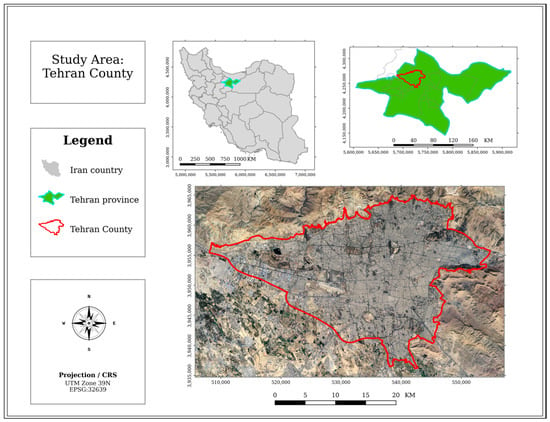
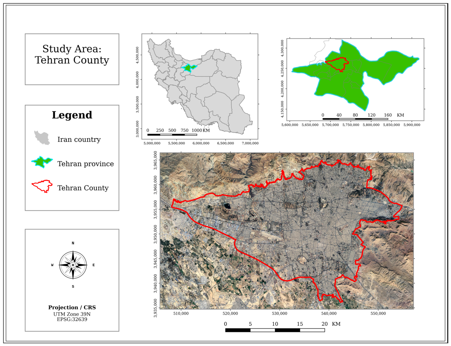
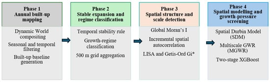
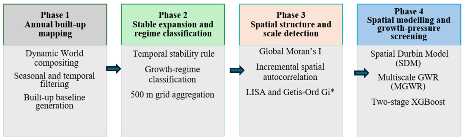
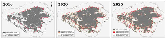
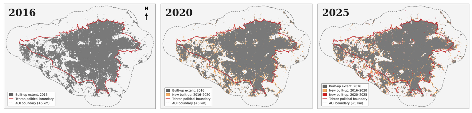
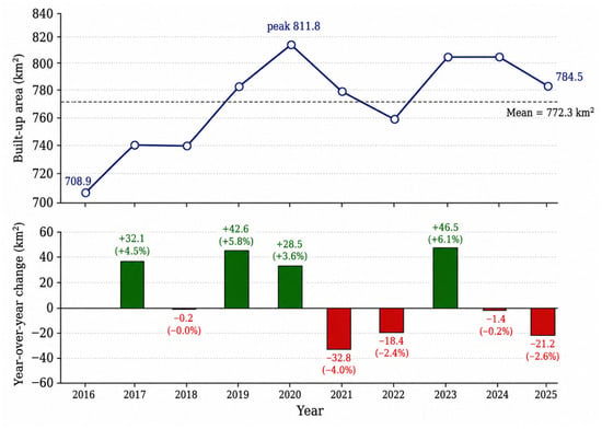
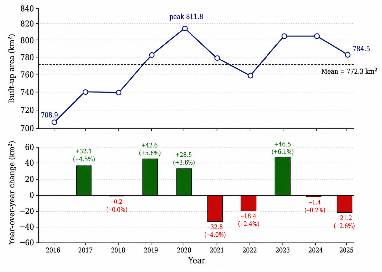
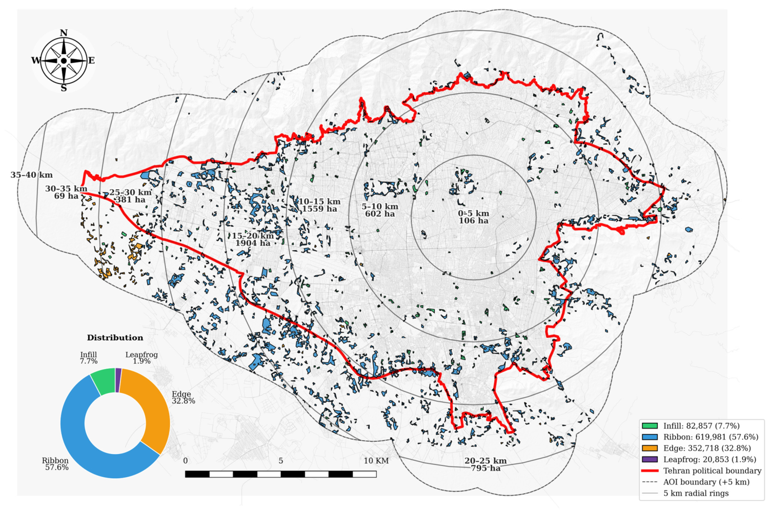
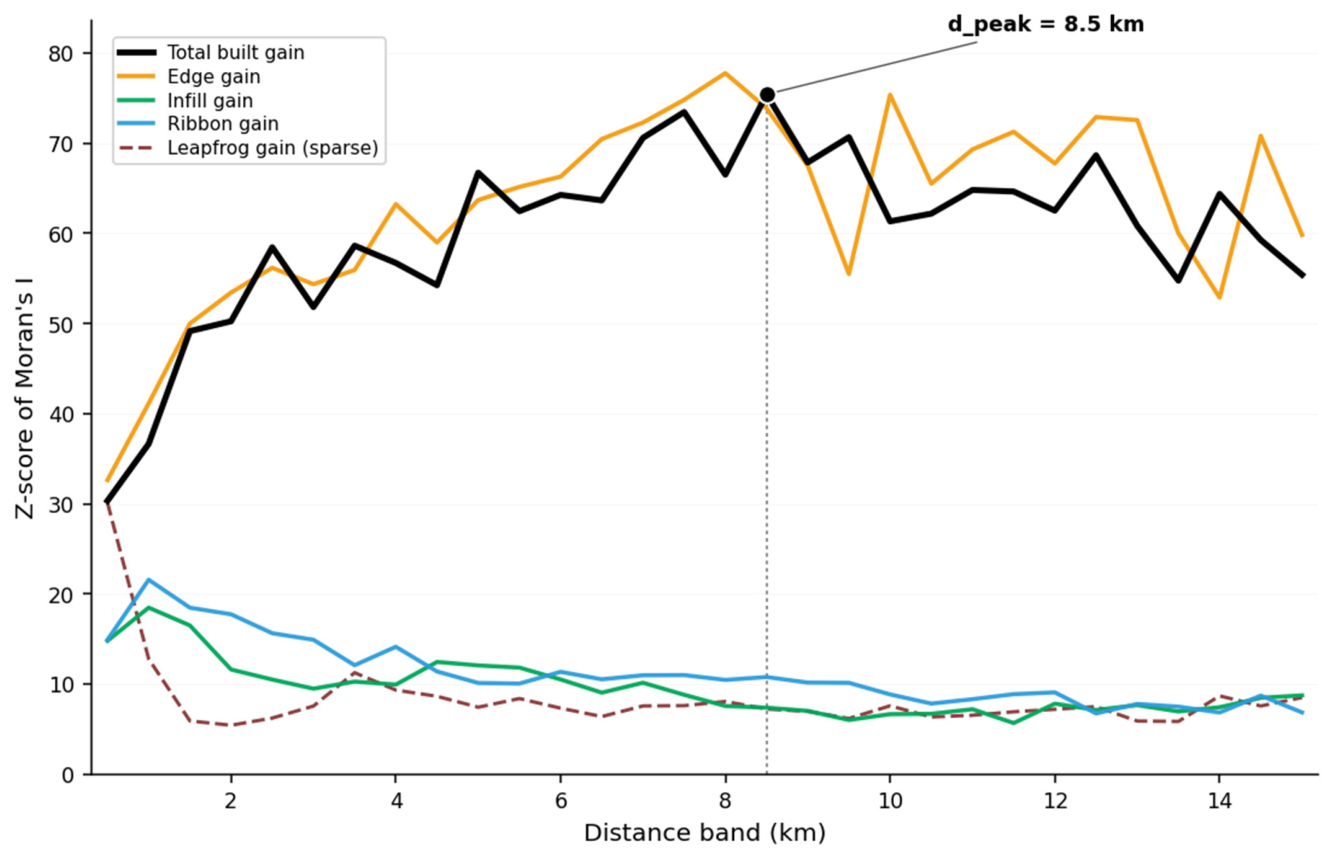
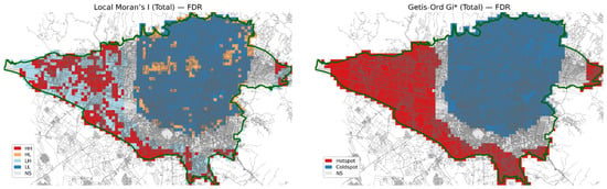
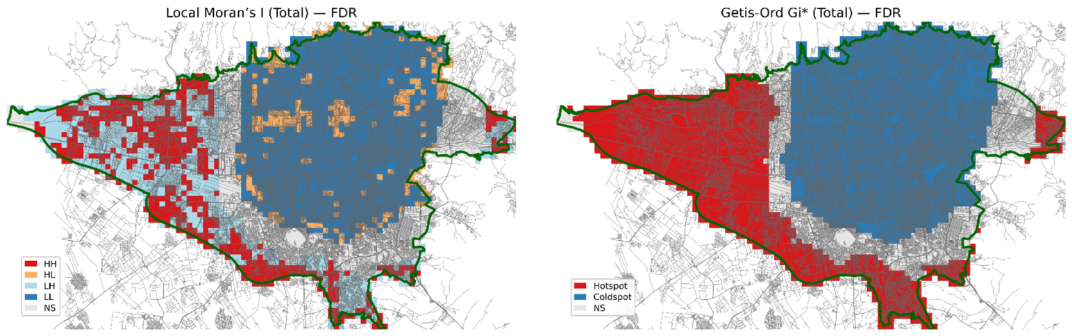
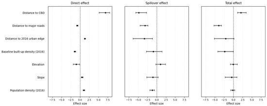
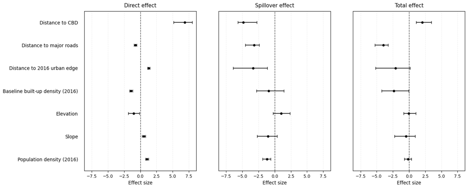
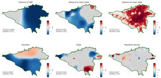
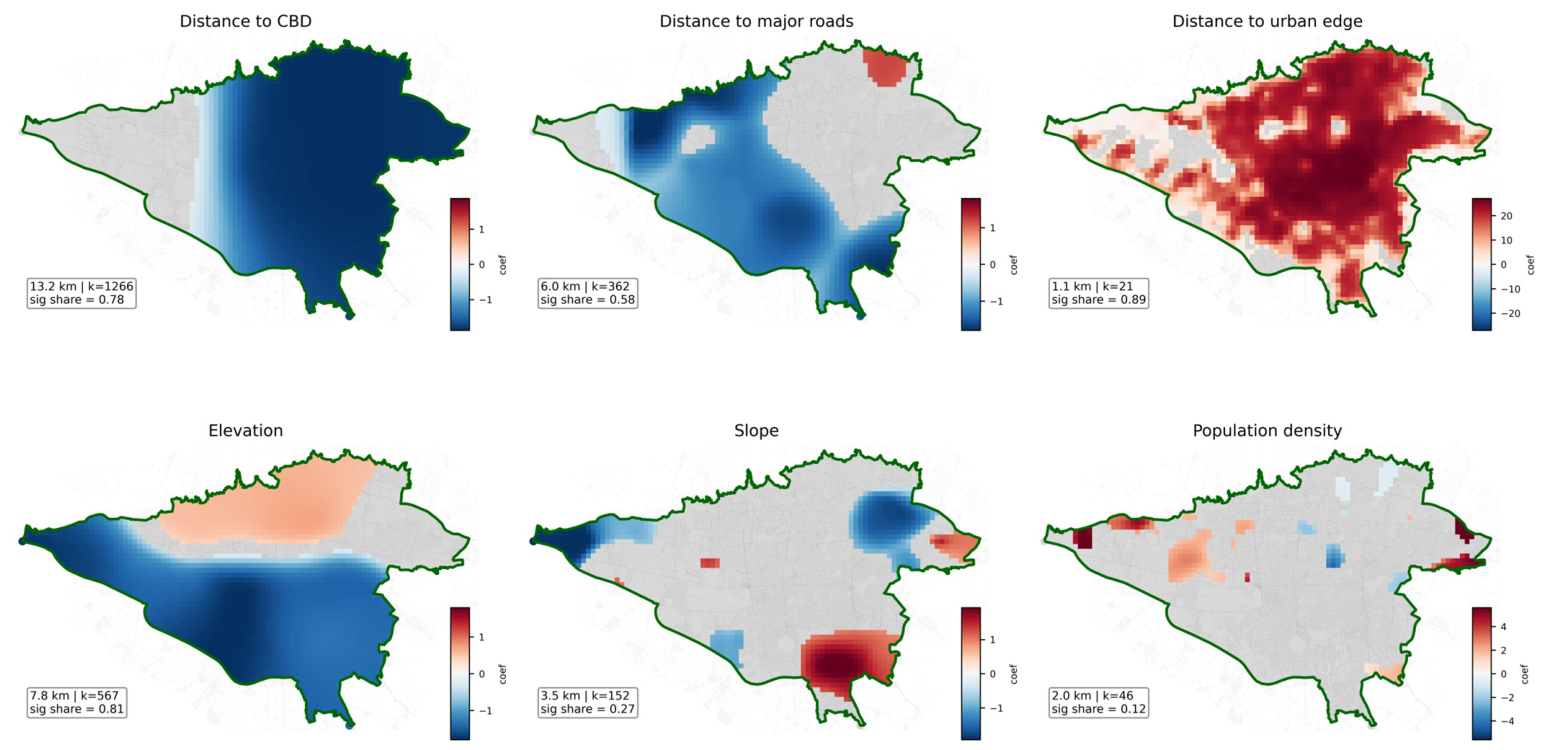
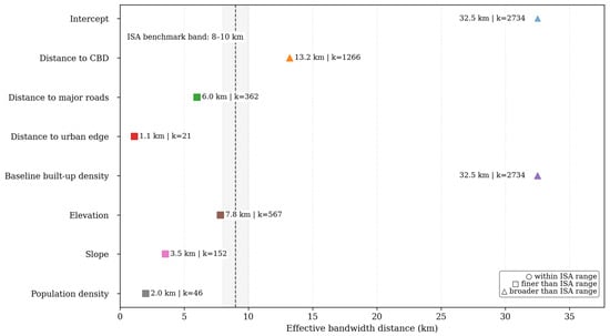
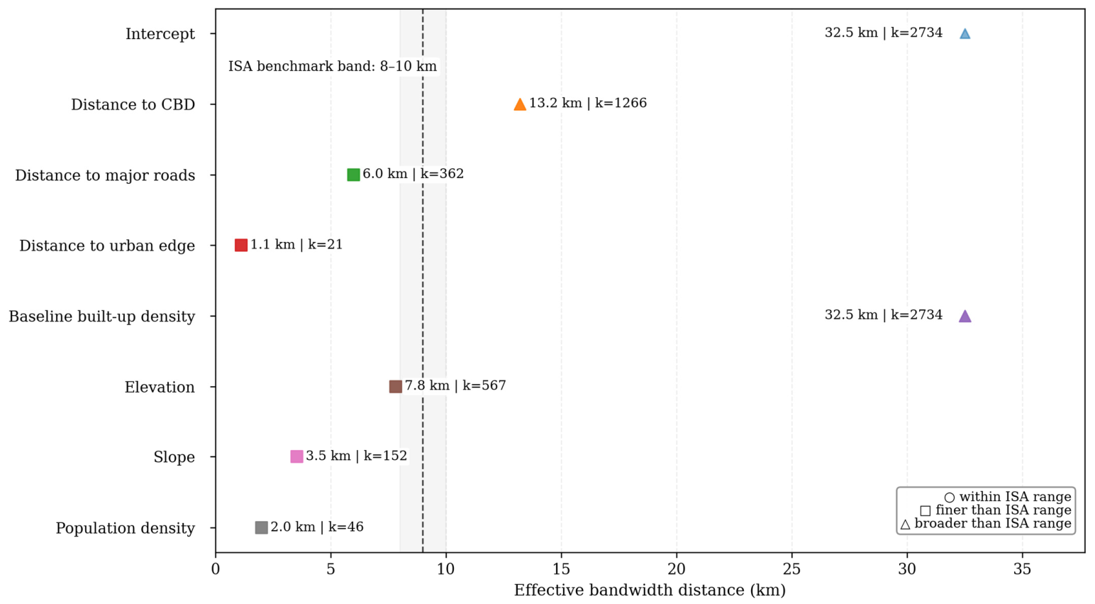
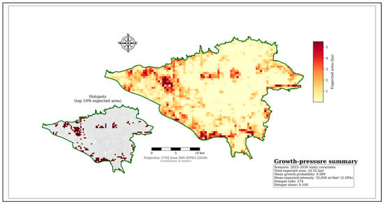
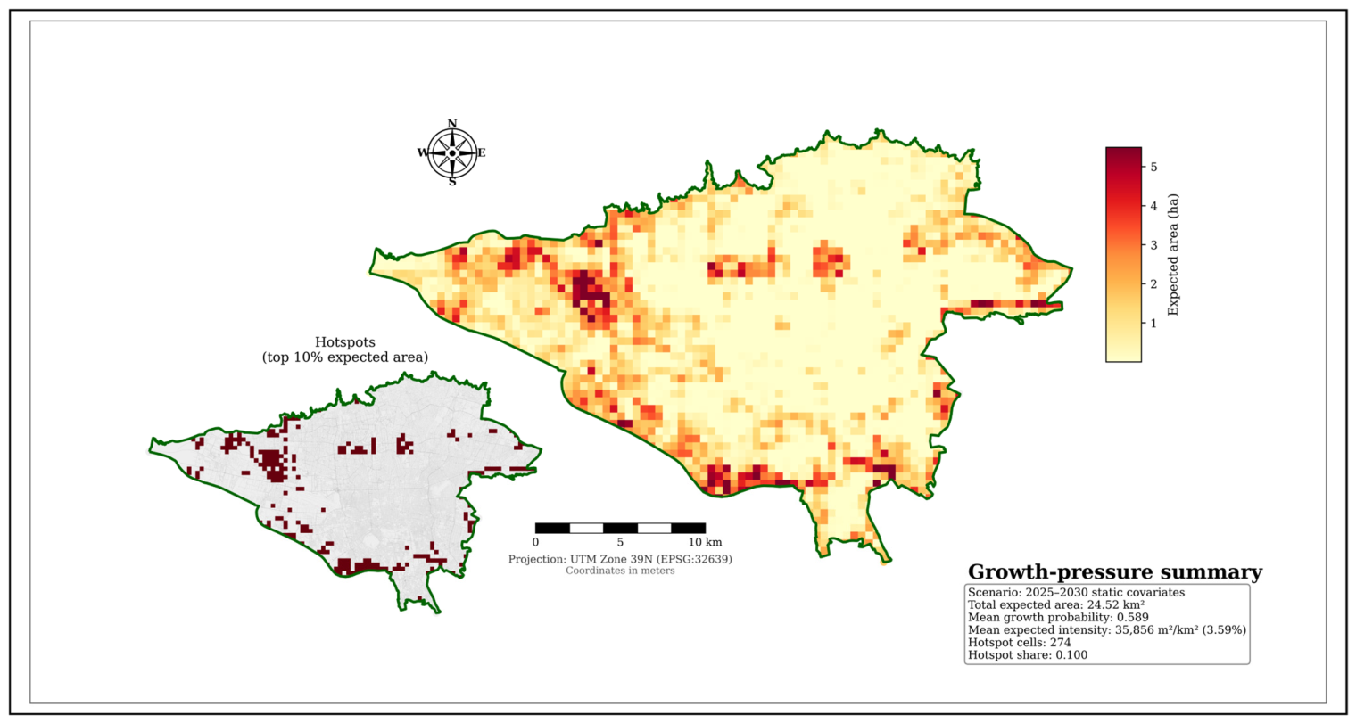
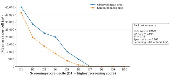
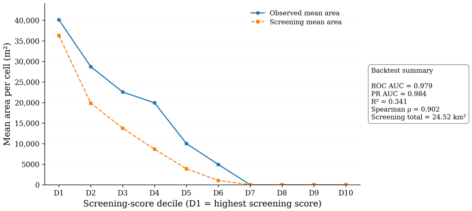

Disclaimer/Publisher’s Note: The statements, opinions and data contained in all publications are solely those of the individual author(s) and contributor(s) and not of MDPI and/or the editor(s). MDPI and/or the editor(s) disclaim responsibility for any injury to people or property resulting from any ideas, methods, instructions or products referred to in the content. |
© 2026 by the authors. Published by MDPI on behalf of the International Society for Photogrammetry and Remote Sensing. Licensee MDPI, Basel, Switzerland. This article is an open access article distributed under the terms and conditions of the Creative Commons Attribution (CC BY) license.