


Abstract
Given the increasing frequency and intensity of floods, which are mostly caused by continuous climate change and growing human pressures on the environment, accurately identifying areas that are susceptible to flooding is a crucial priority for risk reduction and long-term land use planning. Thus, this research examines multilevel flood susceptibility mapping across North Macedonia, using 328 past flood occurrences, 14 conditioning variables derived from a digital elevation model, simplified lithology, and calculated direct runoff. The methodology integrates fuzzy set theory (Fuzzy), analytic hierarchy process (AHP), weighted linear combination (WLC), and random forest (RF) approaches. The two-stage process employs distinct sets of conditioning factors in sequential flood susceptibility mapping: first, generating Fuzzy/AHP/WLC predictions and pseudo-absence data, and second, producing five RF predictions by varying pseudo-absences and binary cutoffs. Validation results indicate that the very high susceptibility class (0.8–1.0) of the Fuzzy/AHP/WLC model predicted 46.6% of flood pixels within 31.6% of the total area. In comparison, the very high susceptibility class of the RF models predicted 88.5%, 78.3%, 60.6%, 48.5%, and 28.3% of flood pixels within 54.7%, 42.2%, 30.5%, 27.0%, and 25.1% of the total area, respectively. The RF models achieved area under the curve (AUC) values exceeding 0.850, with a maximum of 0.966. Additionally, areas of high and low uncertainty were highlighted using a standard deviation map created from the RF models, highlighting agreement/disagreement and potential locations for methodological improvement and focused sampling. The findings also highlight the potential of the multilevel technique for mapping flood susceptibility and call for more research into its potential for future studies and practical uses.
1. Introduction
Flash floods are among the deadliest natural hazards globally. According to estimates by the World Meteorological Organization and related sources, flash floods result in more than 5000 fatalities per year worldwide [1]. Regional analyses also show that specific countries, including the United States, have historically experienced a large proportion of flood-related deaths attributable to flash flooding. For instance, in July 2025, severe flooding in Central Texas led to 134 deaths and significant property damage, with an estimated economic impact of $18 to $22 billion [2]. The floods were caused by intense rainfall and the area’s steep terrain, which increased runoff. Similarly, in September 2024, Asheville, North Carolina, experienced heavy rainfall from Hurricane Helene over already-saturated soils, resulting in 108 fatalities and about $78.8 billion in damages [3,4]. The Valencia Region of Spain, Europe, saw devastating floods in October 2024, resulting in 224 fatalities and significant damage to agriculture and the ecosystem. However, while much of the documented flash flood literature originates from the United States and Western Europe due to data availability, similar hydrometeorological and geomorphic conditions exist in Southeastern Europe, including North Macedonia, where systematic assessments remain limited.
In particular, flash floods pose a significant natural hazard in North Macedonia. This predominantly mountainous country experiences flash floods due to its location in a transition zone across Mediterranean and continental climates, characterized by hot, dry summers and cold, wet (or snowy) winters. Steep slopes, which usually have little vegetation cover that has been weakened by extensive human activity, and low to moderate precipitation with periods of heavy rain occurrences are some of the contributing factors [5,6]. Devastating floods that occurred in and around Skopje, the capital of North Macedonia, in the summer of 2016 caused considerable damage and 23 fatalities due to heavy rainfall that exceeded the monthly normal, with some areas receiving 93 mm in a single day [6]. Hence, assessing flash flood susceptibility is a crucial and essential task in developing a comprehensive plan and ensuring preparedness to address the adverse effects of such a hazard. However, documented event records in the country are sparse, especially in inaccessible mountainous regions that are difficult to reach. Nonetheless, the limitations in data sparsity and the constraints necessary for training and developing effective flash flood models significantly restrict the variety and efficacy of many modeling strategies that can be employed.
Indeed, increased precipitation intensity and frequent downpours due to climate and land use changes are expected to further exacerbate flooding across the globe, including flash floods as well as more widespread river floods [5,7,8,9]. The Intergovernmental Panel on Climate Change’s (IPCC) projects that there is a more than 50% chance that the global temperature rise will reach or surpass 1.5 °C between 2021 and 2040 [10]. For instance, the rise in global temperatures promotes warmer air to hold more water vapor, which fuels extreme downpours, while hardened soils with reduced pore storage prevent water infiltration, leading to runoff, accumulation of standing water, and erosion [11,12]. Additionally, land use changes driven by rapid population and urbanization growth create environmental shifts, including loss of green spaces, deforestation, increased carbon emissions, and urban heat islands that contribute to flooding [9,13,14,15,16]. Thus, addressing the problem of the growing presence and intensity of flood-related hazards caused by climate change and land use activities requires a comprehensive approach that includes robust data collection, sound scientific analysis, collaboration, and other strategies for susceptibility mapping and subsequent disaster preparedness and mitigation.
Therefore, supporting informed decision-making for future land use planning, disaster preparedness, and implementation of green infrastructure requires the development of a flood susceptibility mapping as a critical first step in risk reduction. Many methods and techniques have been proposed to evaluate where or when floods are most likely to occur, some using Geographic Information Systems (GIS) [5,16,17,18,19,20,21,22,23]. Flood inventory maps, which are crucial for flood susceptibility prediction, are often compiled from historical records using various sources, including aerial photography, remote sensing, documentary or media sources, government reports, and meteorological information [24,25,26]. Flood inventory maps serve as the primary record of past flood events, which are then analyzed to understand the relationship between flood conditioning factors and flood occurrences. Common predictive approaches which identify and map areas prone to future flooding include: the flash flood potential index (FFPI), developed by the National Weather Service (NWS), which integrates a number of factors including topography, rainfall, slope, land use, and soil types [27,28,29,30]; a combination of multi-criteria decision analysis (MCDA) and analytical hierarchy process (AHP) [31,32,33,34,35]; statistical models [36,37]; machine learning (ML) models [21,38,39,40,41]; and other hybrid approaches [42,43,44]. Implementation of flood-related models are utilized in various areas such as flood forecasting [28,45], risk assessment [46], flood mitigation and planning [47], and hydrological modeling [30].
Furthermore, many geohazard-related problems, such as floods, are modeled by imperfect observation of the state process [48,49,50]. Such imperfect observation of the state process is associated with significant uncertainties and limitations inherent in measuring, scaling, modeling, and subsequent prediction of flood susceptibility [51]. Additionally, many of the existing approaches apply single-level aggregation methods which may oversimplify complex systems where multilevel or hierarchical relationships exist. For instance, in MCDA, single-level aggregation methods, such as the weighted linear combination (WLC), aggregate all criteria into a single composite score in a single step. In contrast, multilevel or hierarchical methods such as integrative WLC/AHP approaches account for relationships between different levels through implementation of structured analysis, which reduces the complexity of a problem into a hierarchy of goals, criteria, and alternatives before pairwise comparisons and consistency checks for validation of codified judgments are implemented [52,53,54,55,56]. Integrative modeling approaches that use fuzzy sets for combining data and knowledge from diverse sources are advantageous for representing and managing vagueness, imprecision, and uncertainties inherent in the imperfect observation of the state process. For example, expert judgments in AHP can be fuzzified to reflect uncertainties related to observed data, processes that operate at different spatial scales, as well as other subjective choices in the decision-making process. Additional enhancements for identifying hidden patterns, depicting relationships from high-dimensional datasets, and improved predictive power can be achieved by integrating ML algorithms [57,58].
Thus, to overcome the limitations of individual methods (i.e., single-level aggregation) and data sparsity, robust integrative multilevel frameworks that combine advanced techniques like fuzzy sets, physical models, remote sensing, GIS, and ML are needed for effective flood susceptibility mapping. Such frameworks can handle imprecision and vagueness, incorporate diverse data types for flexible, site-specific studies, and enable multiscale computational modeling, thereby improving the accuracy and reliability of the modeling process. Additionally, the flood events occur at different spatial scales from a few 10 s to 100 s of km2, but large-scale national or regional studies face significant challenges and gaps due to a lack of historical records with sufficient detail [32,44,59,60].
Therefore, to leverage the respective strengths of different integrative models, the proposed study in this research aims to assess flood susceptibility across North Macedonia by applying a multilevel approach using fuzzy sets [52,54,61], AHP [53,62,63], weighted linear combination (WLC) [64,65] and random forest (RF), which is a widely used ML technique [21,39,44,66]. Specifically, the main aims of the modeling framework presented here are (1) to transform and standardize criteria (i.e., predictor variables) relevant to flood susceptibility by the fuzzy set theory; (2) to apply AHP for pairwise comparison by elicitation of weights and relative importance of the criteria; (3) to implement flood susceptibility mapping by WLC aggregating the criteria; and (4) to use the WLC flood susceptibility prediction for producing pseudo-absence data in the development of the RF approach. The standardization of the criteria in the first step uses a priori fuzzy membership functions derived from knowledge-driven pattern recognition based on existing flood locations and relationships with the criteria. The next step involves the derivation of a pairwise comparison matrix developed by the goodness of fit between the standardized criteria and the existing floods for assigning the relative importance of the predictor variables. After that, the standardized criteria are aggregated with the AHP weights in the WLC method, which produces a continuous susceptibility index (0–1). Finally, the predicted non-susceptible area from the integrated Fuzzy/AHP/WLC approach is used to generate pseudo-absence data, or locations that have not flooded along the side of the known flood locations (i.e., existing flood inventory database or presence data) as input into the RF model. To further account for uncertainties associated with the classification outcomes into susceptible and non-susceptible areas, different arbitrary cutoff values are used to explore the sensitivity of the Fuzzy/AHP/WLC/RF predictions. The usefulness of this approach is to assist policymakers in better management planning and disaster preparedness through improved prediction at the national scale. The present paper is organized as follows. The study area, materials, and datasets are presented in Section 2 and Section 3. The methods for the modeling approach are highlighted in Section 4, while the results and discussion of the approach are presented in Section 5 and Section 6, and finally, conclusions are offered in Section 7.
2. Study Area
The study area is North Macedonia, a landlocked country located in the central Balkan Peninsula in Southern Europe (Figure 1). The country has diverse climatic regions characterized by a mix of continental and Mediterranean influences. The Vardar Basin, which occupies the plains (i.e., the central region), has a distinct Mediterranean climate with mild winters and hot, dry summers. The mountainous eastern and western regions have a continental climate, with the eastern region having milder winters and hotter, drier summers than the western region. The highly dissected mountainous topography features a wide range of elevations between 50 and 2764 m, and slopes range from 0 to 45°, with an average slope of 15.5°. Annual precipitation ranges from 400 mm at low elevations to more than 1000 mm at high elevations in the western part of the country, with a gradual increase from east to west. Much of the annual precipitation falls as rain and snow during the fall, winter, and spring, while peak stream discharge occurs in late spring and early fall. In recent years, changing precipitation patterns due to climate change have led to more intense and erratic rainfall events over brief time periods, especially during the summer, when temperatures are the highest and the vegetation cover is weak.
Figure 1.
The distribution of recorded floods over the study area. The floods are represented by dark points, whereas dark-blue lines plot the larger rivers. The inset map shows where North Macedonia is situated (i.e., red box) within Europe.
3. Materials and Datasets
3.1. Flood Inventory Database
In North Macedonia, there is an inconsistent spatial and temporal database of historic floods, which gives a misleading impression that flood occurrences are lower, especially in sparsely populated areas. For example, many floods that occur in such isolated and less populated areas are most likely not officially recorded. The existing database used here encompasses a total of 300 prominent floods, including urban, river, and flash floods recorded between 1960 and 2020 [67]. In addition, the existing database was supplemented with 28 flash flood records collected between 1995 and 2020, using field data and newspaper reports [5]. The final flood inventory database in this paper consisted of a total of 328 floods, generated from various sources and mechanisms, including river, urban, and flash floods. The 328 flood points represent approximately 0.00115% of the country’s area (25,713 km2), which is lower than densities reported in many studies of flood susceptibility. However, given the national scope of the investigation, this fraction is reasonable as extensive spatial coverage naturally decreases event density per unit area. Additionally, the floods in the database are represented as points rather than polygons due to a lack of detailed data, which may limit the accuracy and quality of the source data.
3.2. Compilation and Development of Datasets
The Advanced Spaceborne Thermal Emission and Reflection Radiometer (ASTER) Global Digital Elevation Model (GDEM), a publicly available 30 m resolution DEM, was used in the study. The latest version (ASTER GDEM v3) was published in 2019 and reduces voids and water-area anomalies [68]. In this study, the ASTER DEM was projected into the Universal Transverse Mercator (UTM) coordinate system using WGS84 zone 34 N. A total of 14 primary and secondary predictor variables (conditioning factors) were derived from the DEM using the System for Automated Geographical Analysis (SAGA) software version 9.9.1 [69,70]. The primary attributes are computed directly from a DEM and include the first and second derivatives of the elevation surface. Secondary or compound attributes are computed from combinations of two or more primary attributes. The derivatives included: elevation, slope, profile curvature, plane curvature, topographic wetness index (TWI), catchment area, distance to streams, stream power index, channel network distance, topographic position index (TPI), terrain ruggedness index (TRI), LS factor, relative slope position, and valley depth [71,72]. Such computed attributes can be used to quantitatively describe flat, low-lying areas and valleys, which naturally collect water, local surface depressions, water movement, hydrological processes, morphometry, catchment position, and other soil-landscape processes [21,32,44,73,74,75]. For instance, slope affects flooding by influencing the speed and accumulation of water (i.e., the quantity of erosive runoff and the rate of infiltration). The contributing area defines the location of the convergent areas in a landscape that are directly associated with the concentration of surface and subsurface flows, contributing to soil saturation and flood susceptibility. The TWI is used to represent the spatial distribution of water flow across a given area and to predict zones of saturation. On the other hand, the TPI values are used to indicate low-lying areas where water is collected, such as valleys or depressions. The reported TPI values in this work were calculated using a circular neighborhood with a 100 m radius to depict the difference between the elevation of the focal cell and the average elevation of all cells within 100 m. The significance of other attributes lies in characterizing the spatial variability of specific processes occurring in the landscape, which can be tied to potential flood susceptibility.
Additionally, the datasets in this study included simplified lithology and direct runoff computed by the Natural Resource Conservation Service Curve Number (NRCS-CN) method. The lithology was used as a proxy for representing potential permeability and erosion rates, as different rock and soil types act as key controls on the magnitude and frequency of flooding. The lithological map was provided by the Geological Map of North Macedonia at a scale of 1:100,000 [76]. Lastly, the NRCS surface runoff was computed from global land cover and hydrologic soil group maps. The European Space Agency (ESA) WorldCover 2021 was used for the land cover, along with soils that were classified into four hydrologic soil groups (HSGs) for inferring runoff potential [77].
Due to the unavailability of consistent time series in land use and land cover (LULC) datasets for North Macedonia, the ESA WorldCover 2021 dataset (10 m) global LULC layer was used as a reliable proxy for current landscape conditions. Also, to depict the spatial complexity of flood susceptibility, shaped by multiple interacting factors, it was important to integrate different datasets and spatial scales. Therefore, in this paper, a spatial resolution of 30 m was chosen to align with the native DEM resolution, which serves as the main topographic factor in the analysis.
Rather than randomly generating absence data, pseudo-absences were identified using the integrated Fuzzy/AHP/WLC model, which delineated low susceptibility areas to provide informed negative samples for the RF. The development of the integrated Fuzzy/AHP/WLC model used a total of 6 conditioning factors, including channel network distance, topographic position index, terrain ruggedness index, LS factor, relative slope position, and valley depth. The selected conditioning factors are critical to flood susceptibility modeling because they represent hydrological connectivity, runoff concentration, and landscape convergence processes. Locations close to drainage channels, situated in low-lying areas and found on lower slopes or valley-bottom environments, are more susceptible to water buildup and overbank flooding. At the same time, the LS factor and valley depth indicate the efficiency of runoff transport and the confinement of flow, affecting the intensity of flash floods. Collectively, these morphometric parameters capture geomorphological controls governing flood generation and spatial distribution.
This modeling step helped to predict the degree of membership associated with the flood susceptibility, which ranged between 0 (low susceptibility) and 1 (high susceptibility). The flood susceptibility prediction was evaluated using five cutoffs (0.3, 0.4, 0.5, 0.6, and 0.7) to distinguish susceptible from non-susceptible areas. The non-susceptible areas were used for random sampling and development of a total of five pseudo-absence datasets, which were used as inputs in the RF along with the flood inventory database and the rest of the unused conditioning factors.
4. Methods
Figure 2 depicts the necessary datasets and procedural steps involved in the proposed approach. The light blue boxes signify the input data, and the dashed-line boxes divide the dataset inputs into subsets employed at various stages by the multilevel method. The boxes in light yellow illustrate the sequence of models used, while the flood susceptibility results are represented by rounded boxes in light purple. The validation of the resulting flood susceptibility maps and variable importance is depicted in light pink and light green hues.
Figure 2.
Schematic representation of the methodology.
4.1. Fuzzy Sets
Fuzzy set theory [61] is often used for standardizing criteria before they are coupled with the AHP and WLC methods [78,79]. Standardization is a process that transforms and rescales the original criteria so that the membership values range between 0 (full non-membership) and 1 (full membership). Besides the standardization of criteria maps, one of the main goals of the fuzzy membership function is to manage uncertainty and to describe the vagueness of entities in the real world, where belonging to a set is really a matter of degree [78]. For instance, standardization of raster-based conditioning factors uses fuzzy membership functions such as linear, sigmoidal, j-shaped, or other more complex non-monotonic shapes. In the absence of expert knowledge, the standardization is supported by univariate probability density functions (PDF’s) that are codified into fuzzy membership. In this work, PDFs of the six conditioning factors allowed visualization of the distributions of flood occurrences within the total population of floods associated with the individual predictors (Figure 3). The visualization in the figure assisted in the selection of appropriate fuzzy functions and their control points to fit the shape of the fuzzy functions associated with the floods. The type of membership functions and control points used in the study are shown in Table 1. The selection of fuzzy membership functions was guided by the PDFs from the hydrological responses of each variable to flood susceptibility. Variables showing nonlinear threshold behavior (e.g., distance to channel network) were modeled by j-shaped function to reflect rapid susceptibility increase near streams. Gradual terrain transitions (e.g., topographic position index) were represented using a sigmoidal function, while approximately proportional relationships were modeled linearly. Control points (c0, c1, c2, c3) were determined based on the PDFs’ characteristics and geomorphologically relevant thresholds for obtaining realistic transformations. For example, the conditioning factor valley depth was fuzzified by a sigmoidal-symmetric function by the following controlling points (c0, c1, c2, c3), 0, 60, 140, and 350 m using knowledge extracted from the PDF shown in Figure 3f. The fuzzified conditioning factors from Table 1 are shown in Figure 4. As illustrated in the figure, fuzzy membership values are normalized on a continuous scale from 0 (very low susceptibility) to 1 (very high susceptibility), representing the degree of association between each conditioning factor and flood occurrence.
Figure 3.
Distribution of recorded foods within the total population of floods across different conditioning factors (a) channel network distance (CND), (b) topographic position index (TPI), (c) terrain ruggedness index (TRI), (d) LS factor (LS), (e) relative slope position (RSP), and (f) valley depth (VD).
Table 1.
Fuzzy set membership functions and controlling points for the development of flood susceptibility.
4.2. Analytic Hierarchy Process (AHP)
AHP integrates quantitative and qualitative information about decision problems by converting judgments into quantitative values [52,63,78]. The AHP offers a flexible and robust multiple criteria evaluation (MCE) through structured decision-making across multiple criteria, where the complexity of a decision problem is reduced to a sequence of pairwise comparisons. The conditioning factors or criteria are decomposed and synthesized by the AHP’s hierarchical structure into a ratio matrix that provides a clear rationale for ordering the decision alternatives from the most to the least desirable [63]. Specifically, through pairwise comparison of each possible criterion pair, a relative weight for each decision criterion within the hierarchy is derived. Each comparison is a two-part question: which criterion is more important, and by how much. The comparison in this paper uses a five-point scale with values from the set {1/5, 1/4, 1/3, 1/2, 1, 2, 3, 4, 5}, where 1/5 represents the least importance, 1 represents equal importance, and 5 represents the strongest importance. Saaty’s five-point scale is used here, which is a subset of the nine-point (1–9) AHP scale that preserves the ratio properties necessary for AHP while improving the clarity and consistency of pairwise comparisons [80]. The importance of individual conditioning factors for building the flood susceptibility model is illustrated in Figure 5. The figure shows the number of floods that correspond to the degree of membership calculated from the fuzzified conditioning factors. The categorized membership values represent very low to very high flood susceptibility and were used to assess the relative importance of each conditioning factor. For example, Figure 5 shows that a fuzzy membership of 0.7 for the terrain ruggedness index predicts a total of 246 floods, while channel network distance predicts a total of 143 floods. Table 2 presents the pairwise comparison matrix and the scores from the five-point scale for computing the criterion weights. In this paper, the assigned importance in the pairwise comparison was determined by a membership cutoff of 0.7 or higher. This cutoff value was selected because it predicts a relatively high number of flood events and exhibits a consistent trend across all conditioning factors at higher membership. For instance, the average predicted floods with a cutoff higher than 0.7 were 224, 200, 152, 156, 115, and 122 for the terrain ruggedness index, topographic position index, LS factor, valley depth, relative slope position, and channel network distance, respectively. Thus, using the average predicted floods for guidance, in Table 2, the topographic position index (1/2) is equally to moderately less important than the terrain ruggedness index, and the channel network distance (1/4) is moderately to strongly less important than the terrain ruggedness index. The weights for each conditioning factor and the consistency ratio (CR) are also shown in the table. The terrain ruggedness index was assigned the highest relative importance (0.375), followed by the topographic position index (0.223), LS factor (0.131), valley depth (0.112), relative slope position (0.083), and channel network distance (0.074). The value of the CR is 0.017, which is less than 0.10 and indicates good consistency, as shown in Table 2.
Figure 5.
Importance of individual conditioning factors for building the flood susceptibility model. The cutoff used in the AHP matrix was greater than 0.7.
Table 2.
A pairwise comparison matrix for the calculation of criteria weights for flood susceptibility.
4.3. Weighted Linear Combination (WLC)
The WLC method was used to aggregate the fuzzified conditioning factors and calculate the flood suitability score for each location (30 m cell) in the study area. The fuzzified score values in the WLC range between 0 and 1, where 0 is the outcome least susceptible to flooding, and 1 is the outcome most susceptible to flooding. In the WLC method, each criterion (conditioning factor) is multiplied by its weight derived from the pairwise comparison, and the results are summed. The weights of all criteria sum to 1, and the weight of each criterion is inversely proportional to the sum of the other criteria. The degree of membership produced by the fuzzy-based WLC aggregation (Fuzzy/AHP/WLC) ranges between 0 (least susceptible) and 1 (most susceptible). Weights can have a tremendous influence on the solution, as they determine the relative importance of each input variable. By altering the weights, the flood suitability score can be drastically changed to favor specific conditioning factors over others. Thus, the weights in the WLC determine the level of trade-off, where higher criterion weights have more influence on the final suitability scores and can compensate for low criterion scores. Also, when scores from standardized criteria are low while the weights are high, they can only weakly compensate for the poor scores from other criteria [56,65,78].
4.4. Random Forest (RF)
RF is an ensemble of decision trees where individual decision trees are trained with a specific random noise before combined prediction from multiple decision trees is extracted [66]. For classification tasks, the prediction from multiple decision trees is accomplished by majority vote, while for regression tasks, the prediction uses averages from the results of all trees. To improve accuracy and reduce overfitting from the combined prediction, the random decision trees are generated from the training data by a bootstrapping approach, where random subsets of features are selected at each split from the forest. The intent of the bootstrapping and the random split steps in the RF algorithm is to create a collection of diverse and relatively uncorrelated decision trees that subsequently generate robust and accurate final predictions. Additionally, the RF provides measures of predictor-variable importance or contribution to the model’s predictions that can be used to understand complex interactions between predictor variables [21,39,81,82]. Common methods for calculating importance are (1) the mean decrease accuracy method, which randomly permutes the values of a single predictor variable and then evaluates the decreases in prediction accuracy; and (2) mean decrease Gini, which sums the total decrease in node purity associated with a particular variable used in the splitting of the node [83,84,85].
Running the RF algorithm requires both flood (presence) and non-flood (absence) datasets. In this work, the flood inventory database (i.e., the 328 floods) were used as presence, while pseudo-absence data was supported by random sampling throughout the study area using a total of 3500 points that were subjected to binary thresholding based on the Fuzzy/AHP/WLC prediction (i.e., susceptible from non-susceptible areas). A total of five thresholds (i.e., cutoffs) were set at 0.3, 0.4, 0.5, 0.6, and 0.7 degrees of membership, producing five separate datasets containing 712, 1129, 1611, 2199, and 2846 pseudo-absence pixels, respectively. The five separate datasets were used for training and validation of the different RF models. Such an approach was set to increase the variability of the decision trees in the RF model, to reduce generalization error, and to account for uncertainties associated with the arbitrary cutoffs used for the selection of pseudo-absence pixels. The separate training and validation datasets representative of the five cutoffs were generated by stratified random sampling using 70/30% train/test splits. The stratification was implemented to preserve the ratio of presences to absences in the train and test datasets. Also, the weighted RF technique was used to account for the class imbalance (e.g., higher frequency of non-flood pixels) and to improve performance [86].
Specifically, the RF regression algorithm was implemented in R 4.5 software (https://cran.r-project.org). The model was trained with ntree = 1000, mtry = 3 (the square root of the number of conditioning factors), and classwt = (the ratio of the number of flood to the number of non-flood instances). To further reduce uncertainties and improve accuracy, the conditioning factors used for the development of Fuzzy/AHP/WLC were excluded from the RF analysis. The use of different conditioning factors improves flood susceptibility modeling by combining knowledge-driven pattern recognition with hydrological knowledge. The knowledge-driven step relied on hydrologically established variables, whereas the RF step incorporates additional predictors for capturing nonlinear relationships and enhances predictive performance, leading to a more reliable and broadly applicable susceptibility assessment. The input variables used in the RF model included: presence/absence of floods, elevation, slope, profile curvature, plane curvature, topographic wetness index (TWI), catchment area, distance to streams, stream power index, runoff, and lithology. In addition to improve the performance and stability of the RF regression, (1) a log-transform was used to reduce the relative importance of very high values associated with the catchment area; and (2) all conditioning factors were rescaled between 0 and 1 using min-max normalization, which produced a slight improvement in the predictions. Lastly, the probabilistic prediction from the RF regression was evaluated by receiver operating characteristic (ROC) curves and the area under the curve (AUC) measure [44,87,88].
5. Results
5.1. Flood Susceptibility from Fuzzy/AHP/WLC Model
Figure 6a shows the flood susceptibility derived from the Fuzzy/AHP/WLC using the fuzzified conditioning factors from Figure 4 and the criteria weights from Table 2. The figure’s visual representation of flood susceptibility depicts the degree of membership, which varies from 0 to 1, with blue representing low susceptibility (value at or near 0) and dark orange representing high susceptibility (value at or near 1). From this figure, visual patterns show that the highest-susceptibility regions are associated with confined valleys and steep slopes. The combination of narrow valleys with limited floodplains for dispersion of the accumulated river discharge, as well as the steep hills of the mountainsides, causes rainwater to flow quickly over surfaces with destructive speed and force. The figure also shows that the transition zones between the foothills and the plains have the highest susceptibility to flooding. On the other hand, the lowest-susceptibility regions are characterized by higher elevation areas, which are further away from major rivers and streams. For example, the Vardar Basin, which occupies the plains in the central region, shows the highest susceptibility to flooding.
Figure 6.
Flood susceptibility: (a) a map derived by Fuzzy/AHP/WLC by criteria weights from Table 1 and the fuzzified conditioning factors from Figure 4 (the flood occurrences are overlayed and plotted with black circles), and (b) proportion of areas classified by the degree of membership associated with percentage of flood events.
Furthermore, the TRI was the most influential conditioning factor (w1 = 0.375) in the development of the Fuzzy/AHP/WLC model. TRI quantifies the local topographic variation between adjacent neighboring cells in a DEM and reveals potential impacts on surface storage, runoff velocity, and channel routing. Higher TRI values indicate complex terrain and ruggedness, while lower values suggest flatter terrain and a level surface. The controlling points in Table 1 for the development of the flood susceptibility map suggest that TRI was associated with lower values (c0 = 0, c1 = 0.2, c2 = 3, c3 = 6) where excess slow-moving water spread over the surrounding land and caused widespread inundation. The TPI, which is a quantitative measure for assessing the relative position of a location in comparison to the surrounding landscape, was the second most influential conditioning factor (w2 = 0.223). The TPI depicts different landscape features such as ridges, valleys, slopes, and flat terrain. Positive TPI values indicate a location higher than its surroundings (e.g., ridges), while negative values signify a lower position (e.g., valleys or depressions) where water naturally accumulates. The controlling points in Table 1 suggest that TPI was associated with both negative and positive values (c0 = −50, c1 = 0.01, c2 = 0.02, c3 = 40). The remaining morphometric conditioning factors contribute to flood susceptibility by quantifying influences of slope length, slope steepness, distance to regional ridge and valley lines, and proximity to a defined channel network (i.e., overland flow or vertical distances).
The results from Figure 6a are also illustrated in Figure 6b. Figure 6b shows the correctly predicted flood events as a percentage (the dark red line) that corresponds to the area of classified degree of membership, indicating susceptibility generated from the predicted Fuzzy/AHP/WLC approach (the light blue bars). For instance, a good flood susceptibility model will classify most of the floods in the very high susceptibility class of 0.8–1.0 within a small percentage of the total study area. As such, this scenario creates a predictive model that is both accurate (high true positives) and efficient by focusing risk assessment on a limited, high-risk area.
Although that is not the case here, the figure shows that most of the known floods are constricted within a small portion of the study area. For instance, in the figure, a total of 46.7% of the flood events are correctly predicted within 30.9% of the total area that is classified with very high susceptibility of 0.8–1.0. The prediction of the flood events slightly differs by using a lower susceptibility value of 0.7–1.0, where a total of 66.5% of the flood events are correctly predicted within 47.9% of the total area. Thus, applying a cutoff to separate the area into two binary categories (e.g., susceptible vs. non-susceptible) introduces inherent uncertainty, especially for values near the cutoff. The shifts in susceptible and non-susceptible areas introduce uncertainty into the flood mapping and risk assessments, because the boundaries of flood-prone areas are dynamic and make the predictions less reliable, which can impact subsequent environmental management decisions.
In this research, the results from the Fuzzy/AHP/WLC prediction were used to identify locations that represent the absence of floods by excluding areas that were environmentally suitable for floods in the subsequent RF modeling. Thus, the Fuzzy/AHP/WLC prediction was used to produce five binary classifications of susceptible and non-susceptible areas by applying multiple thresholds (i.e., 0.3, 0.4, 0.5, 0.6, and 0.7). While the pseudo-absence flood points were sampled from locations considered non-susceptible areas, the applied thresholds controlled the geographic extents, which yielded a selection of different pseudo-absence datasets. Since pseudo-absence data introduces uncertainty (i.e., a hypothetical absence), a total of five different RF models were produced and used to further understand the model’s performances and related uncertainties introduced by the sampling choice of the pseudo-absence points.
5.2. Flood Susceptibility from RF Models
The predicted flood susceptibility produced by the RF approach is shown in Figure 7 for the five cutoffs used in the modeling. The values from the RF predictions also range from 0 to 1, where blue represents low susceptibility with a value at or near 0, and dark orange represents high susceptibility with a value at or near 1. Compared to the previous Fuzzy/AHP/WLC prediction (Figure 6a), the visual inspection of the RF probability maps (Figure 7) shows resemblance to the spatial pattern, but at higher cutoff values, there is an improved discriminative ability and discernment of susceptibility outcomes. In addition, in Figure 7, noticeable differences are observed in the RF predictive maps regarding the areas occupied by low- and high-susceptibility pixels. The relationship between the RF and the Fuzzy/AHP/WLC predictive models evaluated by R-squared (R2) showed that the degree of similarity was R2 = 0.664, R2 = 0.635, R2 = 0.587, R2 = 0.478, and R2 = 0.398 for the cutoffs of 0.3, 0.4, 0.5, 0.6, and 0.7, respectively.
Figure 7.
RF predictive models produced by five different cutoffs and pseudo-absence datasets derived from the Fuzzy/AHP/WLC prediction. The flood occurrences (i.e., presence points) are overlayed and plotted with black circles.
Figure 8a illustrates the spatial distribution of uncertainties in terms of standard deviation from the models in Figure 7. The standard deviation map provides a spatially explicit measure of the model’s agreement and prediction stability. A high standard deviation denotes areas with higher disagreement and greater variability, whereas a low standard deviation suggests higher agreement and better consistency. The values in the figure illustrate deviation from the mean and range from 0 to 0.5, with lower uncertainties signifying prediction reliability and greater agreement among the RF predictive models. The lowest uncertainties in the figure are found in higher-elevation areas, while the highest uncertainties are associated with lower-elevation areas and transition zones between the foothills and the plains, consistent with the previous observation. The comparative barplot in Figure 8b quantifies the proportion of area and floods associated with different levels of uncertainty. For instance, a total of 28.9% of the total area and a total of 44.0% of the floods are associated with low uncertainties between 0 and 0.1. Indeed, most of the area (71.3%) and floods (88.2%) are contained within the uncertainty range of 0–0.3. The uncertainty map also highlights areas of high and low areas of certainty and subsequently could guide additional sampling efforts. For instance, practitioners can use this map to prioritize additional field verification or data collection in areas where standard deviation exceeds a defined relative cutoff, such as the upper quartile (75th percentile) or areas with standard deviation > 0.3 in normalized susceptibility values (0–1 scale), as shown here. In high-uncertainty zones (i.e., areas with high standard deviation), introducing additional pseudo-absence samples can improve classification stability and reduce sensitivity to cutoff selection.
Figure 8.
(a) Standard deviation from the five RF models from Figure 7, and (b) proportion of uncertainty associated with predicted floods and assigned area. The flood occurrences (i.e., presence points) are overlayed and plotted with black circles.
Figure 9 shows the variable importance for modeling RF flood susceptibility as estimated by the percentage increase in mean squared error (%IncMSE) and increase in node purity (IncNodePurity). The variable importance showed slight variations between the five RF models, although a few predictor variables were consistently shown to be of higher importance in all predictions. The slope was the most significant conditioning factor influencing the spatial distribution of flood susceptibility. The other variables are shown in order of their importance relative to slope, with the x-axis indicating the relative additional model improvement when adding each successive variable. In addition, the node purity (IncNodePurity) shown in sky blue circles represents the decrease in node impurities from splitting a variable taken as the residual sum of squares or variance within a node (i.e., average over all trees). The greater the variable importance, the higher the IncNodePurity value (i.e., larger circles), which are frequently used for splitting nodes and result in homogeneous child nodes and low variance. As with the %IncMSE metric, the slope was the most influential conditioning factor in the initial ranking of the variables used in the RF model. The second most important variable was elevation by both the %IncMSE and the IncNodePurity metrics. The next group of variables with higher importance includes plan curvature, topographic wetness index, and stream power index. The ranking of their variable importance likely changes slightly across the different cutoffs, due to the inherent randomness in the algorithm (i.e., bootstrapping or random subsets). Lastly, the rest of the conditioning factors show similar changes across the different cutoffs except the runoff which shows the lowest variable importance, consistently. Certainly, while runoff is a primary driver of flooding, its lower importance in this study likely reflects methodological and scale-related influences rather than a reduced physical contribution. For example, the NRCS-CN method’s reliance on coarser spatial resolution data likely raises uncertainty due to generalized soil and land cover inputs, as well as generalized variations in local hydrological variability. In contrast, the topographic derivatives generated by the finer DEM resolution show spatial consistency with stronger control over flow accumulation at national scale. It should also be noted that a comparison of variable importance to prior studies is difficult due to the implementation of different methodological approaches, but some similarities exist in the ranking order with a study reported by [88].
Figure 9.
Variable importance plots from the RF models derived by different cutoffs of 0.3, 0.4, 0.5, 0.6, and 0.7.
Figure 10 shows the correctly predicted flood pixels (the dark-yellow bars) and the corresponding susceptible area from the model predictions (the dark-blue bars). For instance, for the RF model with a cutoff of 0.5, a total of 60.6% of the flood pixels are correctly predicted within 30.5% of the total area that is classified under a very high susceptibility class of 0.8–1.0. The predictions for the RF models with cutoffs of 0.6 and 0.7 are slightly different, where a larger proportion of very-low-susceptibility areas is more dominant. For the Fuzzy/AHP/WLC approach, a total of 46.6% of the flood pixels are correctly predicted within 31.6% of the total area that is classified under a very high susceptibility class of 0.8–1.0. Thus, the figure shows that high susceptibility values from both the Fuzzy/AHP/WLC and RF models are associated with greater similarity, while low and moderate susceptibility values are associated with greater dissimilarity. Specifically, the figure suggests that the nature and strength of modeled predictions vary and may be influenced by different factors such as the selection of conditioning factors used, uncertainties due to a lack of complete knowledge used in the fuzzification, the weights assigned to reflect relative importance, and other complexities from the selection of training data, model parameters, overfitting, or imbalanced classes.
Figure 10.
Proportion of correctly predicted floods and assigned area to each susceptibility class from the RF models with cutoffs of 0.3, 0.4, 0.5, 0.6, and 0.7 and the Fuzzy/AHP/WLC approach.
5.3. RF Model Validation
The ROC curves from the five different cutoffs generated by the RF models are shown in Figure 11. The ROC curves were used to evaluate the performance of the trained RF models using unbiased assessments from the test datasets. In addition, the AUC was used to summarize the ROC curve performances for the comparisons of the different RF models produced by the cutoffs. ROC curves plot the false positive rate or specificity (x-axis) and the true positive rate or sensitivity (y-axis) (Figure 11). For example, a true positive is a prediction of a flood for a location where a flood occurred, while a false positive is a prediction of a flood for a location where a flood did not occur. An ideal model would have an AUC equal to 1, because then P (true positive) = 1 and P (false positive) = 0 regardless of the cutoff point [87]. In this study, the overall quantitative index of accuracy corresponds to 0.962, 0.966, 0.946, 0.850, and 0.869 (AUC) for the cutoffs of 0.3, 0.4, 0.5, 0.6, and 0.7, respectively. For instance, for a cutoff value of 0.5 and 0.946 (AUC), the model suggests that there is a 94.6% chance that the model will be able to distinguish between floods and non-floods.
Figure 11.
ROC curves associated with the RF predictive models produced by the five different cutoffs. The diagonal dotted line signifies a random classifier, suggesting a model with a 50% chance of success.
Additional quantitative evaluations for assessing the RF models included root-mean-square error (RMSE), R-squared (R2), and mean absolute error (MAE). The RMSE metric measures the average magnitude of errors between predicted and actual values, the MAE represents the absolute differences between predicted and actual values, and the R2 metric represents the proportion of the variance in the actual data that is explained by the predicted values and represents the goodness of fit. For example, for a cutoff value of 0.5 and R2 = 0.936, about 93.6% of the variance in the actual data (i.e., flood presence/absence) is explained by the predicted values from the RF model. A high R2 value, closer to 1, indicates a strong fit, meaning the predictions from the RF model are close to the actual values. Table 3 shows the accuracy of the flood susceptibility model using three metrics on the test data. The lowest RMSE and MAE values, which indicate a better fit, were associated with the RF cutoff = 0.5. Unlike the RMSE metric, which penalizes larger errors more heavily than smaller errors due to the squaring of the differences, the MAE metric gives equal weight to all errors, regardless of their magnitude.
Table 3.
The RF model performances from the test data were assessed by RMSE, R2, and MAE.
The ROC analysis and the rest of the assessment metrics yield an overall accuracy value that can be associated with different cutoff values, but they do not provide the optimal cutoff values. However, for decision-making purposes, a cutoff value can be selected based on long-term test data, experience, and local knowledge of site-specific issues to guide decision makers in choosing specific cutoffs and the degree of confidence to place in a particular decision. For instance, the right cutoff depends on the situation, where the selection is determined by balancing the performance of false positives (falsely predicted floods) and false negatives (missed floods). Also, one might prioritize high sensitivity if recent cumulative rainfall has left the landscape saturated, while high specificity might be more important if the landscape is unsaturated. As an alternative, a common approach for identifying the optimal cutoff value on the ROC curve (i.e., farthest from the diagonal line) is the Youden index (J), a single statistic that captures the effectiveness of a diagnostic test, calculated as sensitivity plus specificity minus 1 [57,89].
6. Discussion
The results were also examined in the context of previous studies related to flood susceptibility. The obtained findings correspond closely with the existing literature, including [44], which emphasizes that the integration of the MCDA-AHP model and ML models such as Boosted Classification Tree (BCT) and Boosted Regression Tree (BRT) yields varying susceptibility outcomes, and that ML models exceed MCDA-AHP in terms of predictive accuracy. In [44], the MCDA-AHP model categorized about 40% of the basin area into high and very high flood susceptibility categories, while the Fuzzy/AHP/WLC model discussed here classified 31.6% of the area as very high flood susceptibility and accurately identified a total of 46.6% of flood pixels. Both metrics indicate that a large percentage of flood-prone regions are classified into higher susceptibility categories through MCDA GIS methods, even though [44] did not present the percentage of flood pixels. Furthermore, the RF model presented here showed greater predictive capability than the ML methods by [44], identifying over 60% of the observed flood pixels within just 30% of the entire area classified as having very high susceptibility at a cutoff of 0.5, suggesting improved spatial discrimination of flood susceptibility.
The findings of this study also align with recent ML flood susceptibility research, including the work published by [16], which recognized terrain-based factors, especially elevation, proximity to rivers, and hydrological indices as dominant predictors of flooding. However, by using a multilevel modeling strategy, the methodological framework used here goes beyond a strictly data-driven approach. Specifically, the Fuzzy/AHP/WLC framework was first used to generate hydrologically informed pseudo-absence samples at multiple cutoffs, reducing bias associated with randomly generated absence points commonly used in ML studies. In addition, the use of multiple RF models and the derivation of a standard deviation map provide an explicit quantification of spatial prediction uncertainty, which is rarely addressed in comparable studies. Finally, while many ML flood susceptibility assessments are conducted at the watershed scale, the present study applies this multilevel methodology at a national scale, demonstrating its applicability for large-area hazard assessment while preserving interpretability and uncertainty evaluation.
Moreover, the multilevel approach in this study employs both expert knowledge and data-driven modeling for enhancing flood susceptibility mapping. While the expert knowledge step (i.e., Fuzzy/AHP/WLC) addresses the inherent uncertainty and relative importance of flood conditioning factors, the data-driven step (i.e., RF) models the complex, nonlinear relationships between the conditioning factors and historical floods. Additionally, the expert knowledge step creates pseudo-absence points at different cutoffs to support RF predictive flood susceptibility, which also provides decision makers with a standard deviation map that illustrates areas of agreement and disagreement for further methodological enhancements. As such, the high-confidence maps can enhance the identification of high and low susceptibility areas, reduce overfitting, and facilitate sensitivity assessment, resulting in dependable and spatially precise flood susceptibility assessments. Furthermore, the proposed multilevel framework enables the selection of various conditioning factors for various problems under consideration, making it easier to integrate heterogeneous datasets, such as quantitative and qualitative criteria using expert knowledge, and allows for adaptable use across regions with varying data accessibility. The enhanced predictive accuracy shown by the greater percentage of flood pixel identification in smaller susceptible areas also improves spatial precision by this multilevel framework.
Despite its advantages, the multilevel approach has several limitations. First, utilizing fuzzy/AHP/WLC to generate pseudo-absence points relies on expert judgment and the choice of conditioning factors and cutoffs, which could add subjectivity. Second, the accuracy of RF predictions is limited by the availability and spatial resolution of flood inventory and environmental data. For instance, employing point-based flood inventories instead of polygons presents a significant limitation, as it could undervalue the spatial variability and reach of flood occurrences. This simplification might affect model calibration and validation by diminishing the representation of floodplain heterogeneity. Third, the method may not fully account for temporal variability in flooding events, such as seasonal or extreme storm patterns. Finally, while the approach improves spatial precision, it may still overestimate risk in heterogeneous landscapes (i.e., urban environments or topographically diverse areas) where local factors are not fully captured by the input variables.
7. Conclusions
The presented multilevel flood susceptibility mapping framework extends the capabilities of existing spatial models for flood susceptibility, which rely on presence-only data. The importance of the paper sheds light on the targeted derivation of pseudo-absence data through sequential systematic modeling, in which the prediction of flood susceptibility by Fuzzy/AHP/WLC was subjected to different decision cutoffs. The five cutoffs applied to the Fuzzy/AHP/WLC prediction provided varying geographic areas where higher cutoffs generated pseudo-absence points from wider geographic areas, and lower cutoffs generated pseudo-absence points from narrower geographic areas. The combined presence-absence datasets were subsequently used to support the RF predictive flood susceptibility modeling. The results from the multiple predictions susceptibility showed that a derived standard deviation map could be further evaluated for understanding goodness-of-fit and visualization of spatial uncertainties produced by the different cutoffs.
Moreover, the performance of the RF models was assessed by several statistical metrics, including ROC curve analysis and its AUC value, RMSE, R2, and MAE. The AUC values revealed that the values associated with different cutoffs ranged between 0.850 and 0.966 for the testing data. The results from the different cutoffs also showed differences across the classified solutions associated with high and low-susceptibility areas. In addition, the lowest RMSE (0.10371023) and MAE (0.05148084) values that produced the best fit were associated with the RF cutoff = 0.5. At this cutoff, a total of 60.6% of the flood pixels were correctly predicted within 30.5% of the total area classified with a very high susceptibility class of 0.8–1.0. On the other hand, at the same cutoff, the total area of 36.6% was associated only with a total of 2.5% of the flood pixels with a very low susceptibility class of 0–0.2. Notably, the presented approach does not offer an optimal solution or a cutoff value, but local expert knowledge and integration of other susceptibility models can be used in conjunction with the generated outputs by the framework. Regardless of the performances associated with individual cutoff values, the standard deviation map illustrated areas of spatial uncertainty and reliability of the flood susceptibility across the study area. The degree of uncertainty from the five cutoffs showed that most of the area (71.3%) and floods (88.2%) were contained within the uncertainty range of 0–0.3.
In this paper, the selection of conditioning factors was limited to DEM derivatives, lithology, and runoff computed by the NRCS-CN method that were currently available from public sources; thus, we recognize that some key conditioning factors may have been omitted, which could potentially generate different predictive outcomes. Such conditioning factors may include detailed land use/land cover dynamics, soil hydraulic properties (e.g., infiltration capacity and permeability), high-resolution rainfall intensity or storm duration data, groundwater conditions, and flood protection infrastructure such as levees or drainage systems. The inclusion of these factors in future research could improve the representation of hydrological processes and improve the accuracy of flood susceptibility predictions. However, the main focus of these preliminary results was the envisioned implementation of this flexible methodology rather than fully accounting for all possible conditioning factors. The flexible methodology shows a potential blueprint for modification and integration for different study areas or different problems under consideration, using different modules where different strengths and capabilities can be utilized. In future analyses, additional data layers could be derived and estimated, such as datasets from remote sensing (i.e., Landsat, Sentinel, MODIS), climate reanalysis data such as ERA5 and CHIRPS, and near-real-time rainfall weather estimates (i.e., the NOAA Global Forecast System (GFS).
Author Contributions
Conceptualization, Pece V. Gorsevski; methodology, Pece V. Gorsevski; software, Pece V. Gorsevski; validation, Pece V. Gorsevski and Ivica Milevski; formal analysis, Pece V. Gorsevski; resources, Pece V. Gorsevski and Ivica Milevski; data curation, Pece V. Gorsevski and Ivica Milevski; writing—original draft preparation, Pece V. Gorsevski; writing—review and editing, Pece V. Gorsevski and Ivica Milevski; supervision, Pece V. Gorsevski and Ivica Milevski. All authors have read and agreed to the published version of the manuscript.
Funding
This research received no external funding.
Data Availability Statement
The data used in the analysis and presented in this paper are available in the public repositories cited in the text. Further inquiries can be directed to the corresponding author.
Acknowledgments
The authors express gratitude to the three anonymous reviewers for their insightful comments and outstanding additions to the work.
Conflicts of Interest
The authors declare no conflicts of interest.
References
- Flash Flood Guidance System Saves Lives. Available online: https://public.wmo.int/media/news/flash-flood-guidance-system-saves-lives (accessed on 24 February 2026).
- Bach, T. AccuWeather Estimates Texas Floods Will Cost at Least $18 Billion. Available online: https://www.dallasnews.com/business/2025/07/07/accuweather-estimates-texas-floods-will-cost-at-least-18-billion/ (accessed on 26 February 2026).
- Amorim, R.; Villarini, G.; Czajkowski, J.; Smith, J. Flooding from Hurricane Helene and Associated Impacts: A Historical Perspective. J. Hydrol. X 2025, 27, 100204. [Google Scholar] [CrossRef] [Scilit]
- Hertelendy, A.J.; Ciottone, G.R. Averting Flood-Related Deaths and Injuries from Hurricanes: Enhancing Hospital Resilience. Lancet Reg. Health—Am. 2024, 40, 100930. [Google Scholar] [CrossRef] [Scilit] [PubMed]
- Milevski, I.; Aleksova, B.; Valjarević, A.; Gorsevski, P. Cloud-Based Assessment of Flash Flood Susceptibility, Peak Runoff, and Peak Discharge on a National Scale with Google Earth Engine (GEE). Atmosphere 2025, 16, 945. [Google Scholar] [CrossRef] [Scilit]
- Milevski, I. Natural Hazards in the Republic of Macedonia with Special Emphasis on Flood and Earthquake in Skopje in 2016. Geogr. Rev. 2017, 50, 53–69. [Google Scholar]
- Tabari, H. Climate Change Impact on Flood and Extreme Precipitation Increases with Water Availability. Sci. Rep. 2020, 10, 13768. [Google Scholar] [CrossRef] [Scilit]
- Dougherty, E.; Rasmussen, K.L. Changes in Future Flash Flood–Producing Storms in the United States. J. Hydrometeorol. 2020, 21, 2221–2236. [Google Scholar] [CrossRef] [Scilit]
- Gao, G.; Li, J.; Feng, P.; Liu, J.; Wang, Y. Impacts of Climate and Land-Use Change on Flood Events with Different Return Periods in a Mountainous Watershed of North China. J. Hydrol. 2024, 55, 101943. [Google Scholar] [CrossRef] [Scilit]
- Calvin, K.; Dasgupta, D.; Krinner, G.; Mukherji, A.; Thorne, P.W.; Trisos, C.; Romero, J.; Aldunce, P.; Barrett, K.; Blanco, G.; et al. IPCC, 2023: Climate Change 2023: Synthesis Report. Contribution of Working Groups I, II and III to the Sixth Assessment Report of the Intergovernmental Panel on Climate Change; Core Writing Team, Lee, H., Romero, J., Eds.; Intergovernmental Panel on Climate Change (IPCC): Geneva, Switzerland, 2023. [Google Scholar]
- Caplan, J.S.; Giménez, D.; Hirmas, D.R.; Brunsell, N.A.; Blair, J.M.; Knapp, A.K. Decadal-Scale Shifts in Soil Hydraulic Properties as Induced by Altered Precipitation. Sci. Adv. 2019, 5, eaau6635. [Google Scholar] [CrossRef] [Scilit]
- Hsu, H.; Dirmeyer, P.A. Soil Moisture-Evaporation Coupling Shifts into New Gears under Increasing CO2. Nat. Commun. 2023, 14, 1162. [Google Scholar] [CrossRef] [Scilit]
- van Vliet, M.T.H.; Franssen, W.H.P.; Yearsley, J.R.; Ludwig, F.; Haddeland, I.; Lettenmaier, D.P.; Kabat, P. Global River Discharge and Water Temperature under Climate Change. Glob. Environ. Change 2013, 23, 450–464. [Google Scholar] [CrossRef] [Scilit]
- Rogger, M.; Agnoletti, M.; Alaoui, A.; Bathurst, J.C.; Bodner, G.; Borga, M.; Chaplot, V.; Gallart, F.; Glatzel, G.; Hall, J.; et al. Land Use Change Impacts on Floods at the Catchment Scale: Challenges and Opportunities for Future Research. Water Resour. Res. 2017, 53, 5209–5219. [Google Scholar] [CrossRef] [Scilit]
- Moragoda, N.; Cohen, S. Climate-Induced Trends in Global Riverine Water Discharge and Suspended Sediment Dynamics in the 21st Century. Glob. Planet. Change 2020, 191, 103199. [Google Scholar] [CrossRef] [Scilit]
- Khodaei, H.; Nasiri Saleh, F.; Nobakht Dalir, A.; Zarei, E. Future Flood Susceptibility Mapping under Climate and Land Use Change. Sci. Rep. 2025, 15, 12394. [Google Scholar] [CrossRef] [Scilit]
- Popescu, N.-C.; Bărbulescu, A. Flood Hazard Evaluation Using a Flood Potential Index. Water 2023, 15, 3533. [Google Scholar] [CrossRef] [Scilit]
- Aleksova, B.; Milevski, I.; Stefanidis, S. Flash Flood Potential Index at National Scale: Susceptibility Assessment within Catchments. Open Geosci. 2025, 17, 20250891. [Google Scholar] [CrossRef] [Scilit]
- Ebrahimi, E.; Araújo, M.B.; Naimi, B. Flood Susceptibility Mapping to Improve Models of Species Distributions. Ecol. Indic. 2023, 157, 111250. [Google Scholar] [CrossRef] [Scilit]
- Costache, R.; Crăciun, A.; Ciobotaru, N.; Bărbulescu, A. Intelligent Methods for Estimating the Flood Susceptibility in the Danube Delta, Romania. Water 2024, 16, 3511. [Google Scholar] [CrossRef] [Scilit]
- Wahba, M.; Essam, R.; El-Rawy, M.; Al-Arifi, N.; Abdalla, F.; Elsadek, W.M. Forecasting of Flash Flood Susceptibility Mapping Using Random Forest Regression Model and Geographic Information Systems. Heliyon 2024, 10, e33982. [Google Scholar] [CrossRef] [Scilit]
- Rifath, A.R.; Muktadir, M.G.; Hasan, M.; Islam, M.A. Flash Flood Prediction Modeling in the Hilly Regions of Southeastern Bangladesh: A Machine Learning Attempt on Present and Future Climate Scenarios. Environ. Chall. 2024, 17, 101029. [Google Scholar] [CrossRef] [Scilit]
- Tikuye, B.G.; Ray, R.L.; Abeysingha, N.S.; Gurau, S. Integrating Multi-Criteria Decision Analysis and Geospatial Data for Flood Susceptibility Mapping in Texas, USA. Prog. Disaster Sci. 2025, 28, 100462. [Google Scholar] [CrossRef] [Scilit]
- Puech, C.; Raclot, D. Using Geographical Information Systems and Aerial Photographs to Determine Water Levels during Floods. Hydrol. Process. 2002, 16, 1593–1602. [Google Scholar] [CrossRef] [Scilit]
- Diakakis, M. An Inventory of Flood Events in Athens, Greece, during the Last 130 Years. Seasonality and Spatial Distribution. J. Flood Risk Manag. 2014, 7, 332–343. [Google Scholar] [CrossRef] [Scilit]
- Archer, D.; O’Donnell, G.; Lamb, R.; Warren, S.; Fowler, H.J. Historical Flash Floods in England: New Regional Chronologies and Database. J. Flood Risk Manag. 2019, 12, e12526. [Google Scholar] [CrossRef] [Scilit]
- Gorsevski, P.V.; Gessler, P.E.; Boll, J.; Elliot, W.J.; Foltz, R.B. Spatially and Temporally Distributed Modeling of Landslide Susceptibility. Geomorphology 2006, 80, 178–198. [Google Scholar] [CrossRef] [Scilit]
- Looper, J.P.; Vieux, B.E. An Assessment of Distributed Flash Flood Forecasting Accuracy Using Radar and Rain Gauge Input for a Physics-Based Distributed Hydrologic Model. J. Hydrol. 2012, 412–413, 114–132. [Google Scholar] [CrossRef] [Scilit]
- Jehanzaib, M.; Ajmal, M.; Achite, M.; Kim, T.-W. Comprehensive Review: Advancements in Rainfall-Runoff Modelling for Flood Mitigation. Climate 2022, 10, 147. [Google Scholar] [CrossRef] [Scilit]
- Boithias, L.; Sauvage, S.; Lenica, A.; Roux, H.; Abbaspour, K.C.; Larnier, K.; Dartus, D.; Sánchez-Pérez, J.M. Simulating Flash Floods at Hourly Time-Step Using the SWAT Model. Water 2017, 9, 929. [Google Scholar] [CrossRef] [Scilit]
- Rincón, D.; Khan, U.T.; Armenakis, C. Flood Risk Mapping Using GIS and Multi-Criteria Analysis: A Greater Toronto Area Case Study. Geosciences 2018, 8, 275. [Google Scholar] [CrossRef] [Scilit]
- Santos, P.P.; Reis, E.; Pereira, S.; Santos, M. A Flood Susceptibility Model at the National Scale Based on Multicriteria Analysis. Sci. Total Environ. 2019, 667, 325–337. [Google Scholar] [CrossRef] [Scilit]
- Pourghasemi, H.R.; Gayen, A.; Panahi, M.; Rezaie, F.; Blaschke, T. Multi-Hazard Probability Assessment and Mapping in Iran. Sci. Total Environ. 2019, 692, 556–571. [Google Scholar] [CrossRef] [Scilit] [PubMed]
- El-Rawy, M.; Elsadek, W.M.; De Smedt, F. Flood Hazard Assessment and Mitigation Using a Multi-Criteria Approach in the Sinai Peninsula, Egypt. Nat. Hazards 2023, 115, 215–236. [Google Scholar] [CrossRef] [Scilit]
- Bunmi Mudashiru, R.; Sabtu, N.; Abdullah, R.; Saleh, A.; Abustan, I. Optimality of Flood Influencing Factors for Flood Hazard Mapping: An Evaluation of Two Multi-Criteria Decision-Making Methods. J. Hydrol. 2022, 612, 128055. [Google Scholar] [CrossRef] [Scilit]
- Khosravi, K.; Pourghasemi, H.R.; Chapi, K.; Bahri, M. Flash Flood Susceptibility Analysis and Its Mapping Using Different Bivariate Models in Iran: A Comparison between Shannon’s Entropy, Statistical Index, and Weighting Factor Models. Environ. Monit. Assess. 2016, 188, 656. [Google Scholar] [CrossRef] [Scilit]
- Chowdhury, M.S. Flash Flood Susceptibility Mapping of North-East Depression of Bangladesh Using Different GIS Based Bivariate Statistical Models. Watershed Ecol. Environ. 2024, 6, 26–40. [Google Scholar] [CrossRef] [Scilit]
- Yu, H.; Luo, Z.; Wang, L.; Ding, X.; Wang, S. Improving the Accuracy of Flood Susceptibility Prediction by Combining Machine Learning Models and the Expanded Flood Inventory Data. Remote Sens. 2023, 15, 3601. [Google Scholar] [CrossRef] [Scilit]
- Tan, X.Z.; Li, Y.; Wu, X.X.; Dai, C.; Zhang, X.L.; Cai, Y.P. Identification of the Key Driving Factors of Flash Flood Based on Different Feature Selection Techniques Coupled with Random Forest Method. J. Hydrol. 2024, 51, 101624. [Google Scholar] [CrossRef] [Scilit]
- Soares, J.A.J.P.; Ozelim, L.C.S.M.; Bacelar, L.; Ribeiro, D.B.; Stephany, S.; Santos, L.B.L. ML4FF: A Machine-Learning Framework for Flash Flood Forecasting Applied to a Brazilian Watershed. J. Hydrol. 2025, 652, 132674. [Google Scholar] [CrossRef] [Scilit]
- Liu, Z.; Felton, T.; Mostafavi, A. Interpretable Machine Learning for Predicting Urban Flash Flood Hotspots Using Intertwined Land and Built-Environment Features. Comput. Environ. Urban Syst. 2024, 110, 102096. [Google Scholar] [CrossRef] [Scilit]
- Costache, R.; Pham, Q.B.; Avand, M.; Thuy Linh, N.T.; Vojtek, M.; Vojteková, J.; Lee, S.; Khoi, D.N.; Thao Nhi, P.T.; Dung, T.D. Novel Hybrid Models between Bivariate Statistics, Artificial Neural Networks and Boosting Algorithms for Flood Susceptibility Assessment. J. Environ. Manag. 2020, 265, 110485. [Google Scholar] [CrossRef] [Scilit]
- Akay, H. Flood Susceptibility Mapping Using Information Fusion Paradigm Integrated with Decision Trees. Water Resour. Manag. 2024, 38, 5365–5383. [Google Scholar] [CrossRef] [Scilit]
- Vojtek, M.; Vojteková, J.; Costache, R.; Pham, Q.B.; Lee, S.; Arshad, A.; Sahoo, S.; Linh, N.T.T.; Anh, D.T. Comparison of Multi-Criteria-Analytical Hierarchy Process and Machine Learning-Boosted Tree Models for Regional Flood Susceptibility Mapping: A Case Study from Slovakia. Geomat. Nat. Hazards Risk 2021, 12, 1153–1180. [Google Scholar] [CrossRef] [Scilit]
- Wu, J.; Liu, H.; Wei, G.; Song, T.; Zhang, C.; Zhou, H. Flash Flood Forecasting Using Support Vector Regression Model in a Small Mountainous Catchment. Water 2019, 11, 1327. [Google Scholar] [CrossRef] [Scilit]
- Yildirim, E.; Just, C.; Demir, I. Flood Risk Assessment and Quantification at the Community and Property Level in the State of Iowa. Int. J. Disaster Risk Reduct. 2022, 77, 103106. [Google Scholar] [CrossRef] [Scilit]
- Griffiths, J.; Borne, K.E.; Semadeni-Davies, A.; Tanner, C.C. Selection, Planning, and Modelling of Nature-Based Solutions for Flood Mitigation. Water 2024, 16, 2802. [Google Scholar] [CrossRef] [Scilit]
- Shimadzu, H.; Foster, S.D.; Darnell, R. Imperfect Observations in Ecological Studies. Environ. Ecol. Stat. 2016, 23, 337–358. [Google Scholar] [CrossRef] [Scilit]
- Bulgin, C.E.; Thomas, C.M.; Waller, J.A.; Woolliams, E.R. Representation Uncertainty in the Earth Sciences. Earth Space Sci. 2022, 9, e2021EA002129. [Google Scholar] [CrossRef] [Scilit]
- Ohnesorge, M.; Watkins, A. What Is Philosophy of the Geosciences? Philos. Compass 2024, 19, e12962. [Google Scholar] [CrossRef] [Scilit]
- Gorsevski, P.V. Predicted Streamflow Sensitivity to Climate Change Using TOPMODEL with CLIGEN Weather Generator in a Data-Sparse Medium-Sized Mediterranean Watershed. Water Resour. Manag. 2026, 40, 152. [Google Scholar] [CrossRef] [Scilit]
- Gorsevski, P.V.; Jankowski, P.; Gessler, P.E. An Heuristic Approach for Mapping Landslide Hazard by Integrating Fuzzy Logic with Analytic Hierarchy Process. Control Cybern. 2006, 35, 121–146. [Google Scholar]
- Gorsevski, P.V.; Gessler, P.E.; Jankowski, P. Integrating a Fuzzy k -Means Classification and a Bayesian Approach for Spatial Prediction of Landslide Hazard. J. Geogr. Syst. 2003, 5, 223–251. [Google Scholar] [CrossRef] [Scilit]
- Gorsevski, P.V.; Jankowski, P. An Optimized Solution of Multi-Criteria Evaluation Analysis of Landslide Susceptibility Using Fuzzy Sets and Kalman Filter. Comput. Geosci. 2010, 36, 1005–1020. [Google Scholar] [CrossRef] [Scilit]
- Gorsevski, P.V.; Jankowski, P. Discerning Landslide Susceptibility Using Rough Sets. Comput. Environ. Urban Syst. 2008, 32, 53–65. [Google Scholar] [CrossRef] [Scilit]
- Liu, X.; Gorsevski, P.V.; Yacobucci, M.M.; Onasch, C.M. A Web-Based Multicriteria Evaluation of Spatial Trade-Offs between Environmental and Economic Implications from Hydraulic Fracturing in a Shale Gas Region in Ohio. Environ. Monit. Assess. 2016, 188, 376. [Google Scholar] [CrossRef] [Scilit]
- Zerai, F.T.; Gorsevski, P.V.; Panter, K.S.; Farver, J.; Tangestani, M.H. Integration of ASTER and Soil Survey Data by Principal Components Analysis and One-Class Support Vector Machine for Mineral Prospectivity Mapping in Kerkasha, Southwestern Eritrea. Nat. Resour. Res. 2023, 32, 2463–2493. [Google Scholar] [CrossRef] [Scilit]
- Shayeganpour, S.; Tangestani, M.H.; Gorsevski, P.V. Machine Learning and Multi-Sensor Data Fusion for Mapping Lithology: A Case Study of Kowli-Kosh Area, SW Iran. Adv. Space Res. 2021, 68, 3992–4015. [Google Scholar] [CrossRef] [Scilit]
- Modrick, T.M.; Georgakakos, K.P. The Character and Causes of Flash Flood Occurrence Changes in Mountainous Small Basins of Southern California under Projected Climatic Change. J. Hydrol. 2015, 3, 312–336. [Google Scholar] [CrossRef] [Scilit]
- Saharia, M.; Kirstetter, P.-E.; Vergara, H.; Gourley, J.J.; Emmanuel, I.; Andrieu, H. On the Impact of Rainfall Spatial Variability, Geomorphology, and Climatology on Flash Floods. Water Resour. Res. 2021, 57, e2020WR029124. [Google Scholar] [CrossRef] [Scilit]
- Zadeh, L.A. Fuzzy Sets. Inf. Control 1965, 8, 338–353. [Google Scholar] [CrossRef] [Scilit]
- Gorsevski, P.V.; Jankowski, P.; Gessler, P.E. Spatial Prediction of Landslide Hazard Using Fuzzy K-Means and Dempster-Shafer Theory. Trans. GIS 2005, 9, 455–474. [Google Scholar] [CrossRef] [Scilit]
- Saaty, R.W. The Analytic Hierarchy Process—What It Is and How It Is Used. Math. Model. 1987, 9, 161–176. [Google Scholar] [CrossRef] [Scilit]
- Gorsevski, P.V.; Cathcart, S.C.; Mirzaei, G.; Jamali, M.M.; Ye, X.; Gomezdelcampo, E. A Group-Based Spatial Decision Support System for Wind Farm Site Selection in Northwest Ohio. Energy Policy 2013, 55, 374–385. [Google Scholar] [CrossRef] [Scilit]
- Gorsevski, P.V.; Donevska, K.R.; Mitrovski, C.D.; Frizado, J.P. Integrating Multi-Criteria Evaluation Techniques with Geographic Information Systems for Landfill Site Selection: A Case Study Using Ordered Weighted Average. Waste Manag. 2012, 32, 287–296. [Google Scholar] [CrossRef] [Scilit]
- Breiman, L. Random Forests. Mach. Learn. 2001, 45, 5–32. [Google Scholar] [CrossRef] [Scilit]
- Dumova-Jovanovska, E.; Cvetovska, M.; Čurilov, S.; Milkova, K.; Bogoevska, S.; Jovanoska Mitrevska, M.; Donevska, K.; Gješovska, V.; Ilioski, B.; Jovanovski, M. Study for the Spatial Plan of the Republic of North Macedonia: Natural and Technical Technological Disasters; Tech. No. A91923; Ministry of Environment and Spatial Planning: Skopje, North Macedonia, 2023.
- Abrams, M.; Crippen, R.; Fujisada, H. ASTER Global Digital Elevation Model (GDEM) and ASTER Global Water Body Dataset (ASTWBD). Remote Sens. 2020, 12, 1156. [Google Scholar] [CrossRef] [Scilit]
- Conrad, O.; Bechtel, B.; Bock, M.; Dietrich, H.; Fischer, E.; Gerlitz, L.; Wehberg, J.; Wichmann, V.; Böhner, J. System for Automated Geoscientific Analyses (SAGA) v. 2.1.4. Geosci. Model Dev. 2015, 8, 1991–2007. [Google Scholar] [CrossRef] [Scilit]
- SAGA System for Automated Geoscientific Analyses (SAGA) GIS. Available online: http://www.saga-gis.org/en/index.html (accessed on 4 March 2026).
- Wilson, J.; Gallant, J. Terrain Analysis: Principles and Applications; John Wiley & Sons, Inc.: Hoboken, NJ, USA, 2000. [Google Scholar]
- Hengl, T.; Reuter, H.I. Geomorphometry: Concepts, Software, Applications; Newnes: Oxford, UK, 2008; ISBN 978-0-08-092188-4. [Google Scholar]
- Tarboton, D.G. A New Method for the Determination of Flow Directions and Upslope Areas in Grid Digital Elevation Models. Water Resour. Res. 1997, 33, 309–319. [Google Scholar] [CrossRef] [Scilit]
- O’Loughlin, E.M. Prediction of Surface Saturation Zones in Natural Catchments by Topographic Analysis. Water Resour. Res. 1986, 22, 794–804. [Google Scholar] [CrossRef] [Scilit]
- Moore, I.D.; Grayson, R.B.; Ladson, A.R. Digital Terrain Modelling: A Review of Hydrological, Geomorphological, and Biological Applications. Hydrol. Process. 1991, 5, 3–30. [Google Scholar] [CrossRef] [Scilit]
- Federal Geological Survey of SFRY. Interpreter of the Basic Geological Map of Socialist Federal Republic of Yugoslavia 1:100,000 (Sheet 25 for SR Macedonia); Prof. Fund Fed. Geol. Surv. SFRY: Belgrade, Yugoslavia, 1963–1985. (In Macedonian) [Internal map] 1985 [Google Scholar]
- Ross, C.W.; Prihodko, L.; Anchang, J.; Kumar, S.; Ji, W.; Hanan, N.P. HYSOGs250m, Global Gridded Hydrologic Soil Groups for Curve-Number-Based Runoff Modeling. Sci. Data 2018, 5, 180091. [Google Scholar] [CrossRef] [Scilit]
- Malczewski, J. GIS and Multicriteria Decision Analysis; Wiley: New York, NY, USA, 1999. [Google Scholar]
- Malczewski, J.; Rinner, C. Multicriteria Decision Analysis in Geographic Information Science; Advances in Geographic Information Science; Springer: Berlin/Heidelberg, Germany, 2015. [Google Scholar]
- Schmidt, K.; Aumann, I.; Hollander, I.; Damm, K.; von der Schulenburg, J.-M.G. Applying the Analytic Hierarchy Process in Healthcare Research: A Systematic Literature Review and Evaluation of Reporting. BMC Med. Inf. Decis. Mak. 2015, 15, 112. [Google Scholar] [CrossRef] [Scilit] [PubMed]
- Maxwell, A.E.; Warner, T.A.; Strager, M.P. Predicting Palustrine Wetland Probability Using Random Forest Machine Learning and Digital Elevation Data-Derived Terrain Variables. Photogramm. Eng. Remote Sens. 2016, 82, 437–447. [Google Scholar] [CrossRef] [Scilit]
- Esfandiari, M.; Jabari, S.; McGrath, H.; Coleman, D. Flood Mapping Using Random Forest and Identifying the Essential Conditioning Factors; a Case Study in Fredericton, New Brunswick, Canada. ISPRS Ann. Photogramm. Remote Sens. Spat. Inf. Sci. 2020, V-3–2020, 609–615. [Google Scholar] [CrossRef] [Scilit]
- Strobl, C.; Boulesteix, A.-L.; Zeileis, A.; Hothorn, T. Bias in Random Forest Variable Importance Measures: Illustrations, Sources and a Solution. BMC Bioinform. 2007, 8, 25. [Google Scholar] [CrossRef] [Scilit]
- Menze, B.H.; Kelm, B.M.; Masuch, R.; Himmelreich, U.; Bachert, P.; Petrich, W.; Hamprecht, F.A. A Comparison of Random Forest and Its Gini Importance with Standard Chemometric Methods for the Feature Selection and Classification of Spectral Data. BMC Bioinform. 2009, 10, 213. [Google Scholar] [CrossRef] [Scilit]
- Dunne, R.; Reguant, R.; Ramarao-Milne, P.; Szul, P.; Sng, L.M.F.; Lundberg, M.; Twine, N.A.; Bauer, D.C. Thresholding Gini Variable Importance with a Single-Trained Random Forest: An Empirical Bayes Approach. Comput. Struct. Biotechnol. J. 2023, 21, 4354–4360. [Google Scholar] [CrossRef] [Scilit]
- Benkendorf, D.J.; Schwartz, S.D.; Cutler, D.R.; Hawkins, C.P. Correcting for the Effects of Class Imbalance Improves the Performance of Machine-Learning Based Species Distribution Models. Ecol. Model. 2023, 483, 110414. [Google Scholar] [CrossRef] [Scilit]
- Gorsevski, P.V. A Free Web-Based Approach for Rainfall-Induced Landslide Susceptibility Modeling: Case Study of Clearwater National Forest, Idaho, USA. Environ. Model. Softw. 2023, 161, 105632. [Google Scholar] [CrossRef] [Scilit]
- Ali, S.A.; Parvin, F.; Vojteková, J.; Costache, R.; Linh, N.T.T.; Pham, Q.B.; Vojtek, M.; Gigović, L.; Ahmad, A.; Ghorbani, M.A. GIS-Based Landslide Susceptibility Modeling: A Comparison between Fuzzy Multi-Criteria and Machine Learning Algorithms. Geosci. Front. 2021, 12, 857–876. [Google Scholar] [CrossRef] [Scilit]
- Youden, W.J. Index for Rating Diagnostic Tests. Cancer 1950, 3, 32–35. [Google Scholar] [CrossRef]
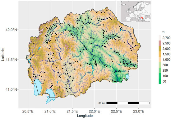
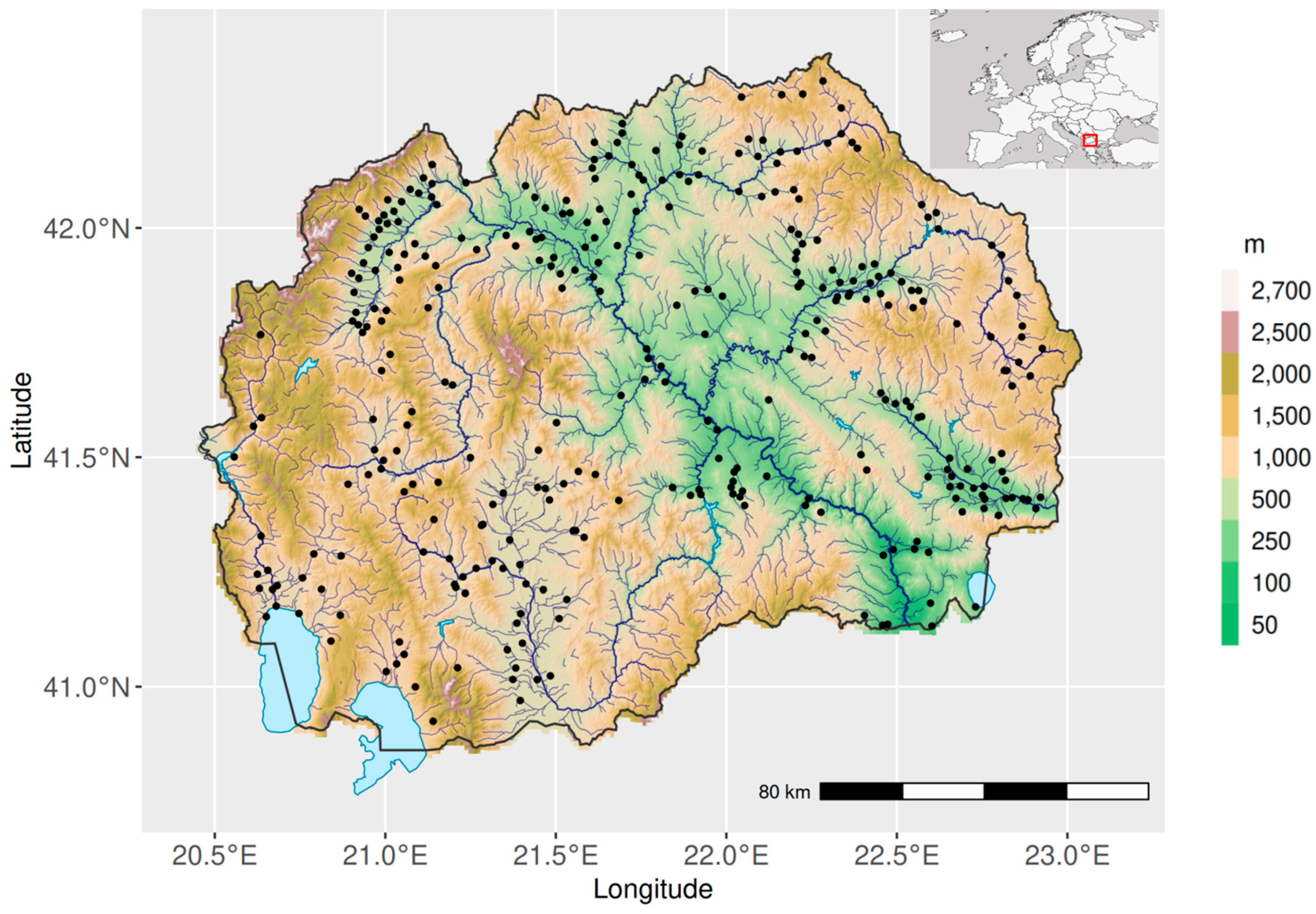
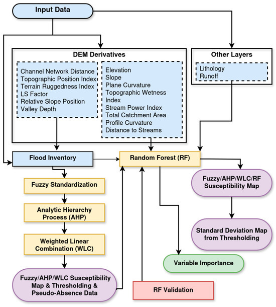
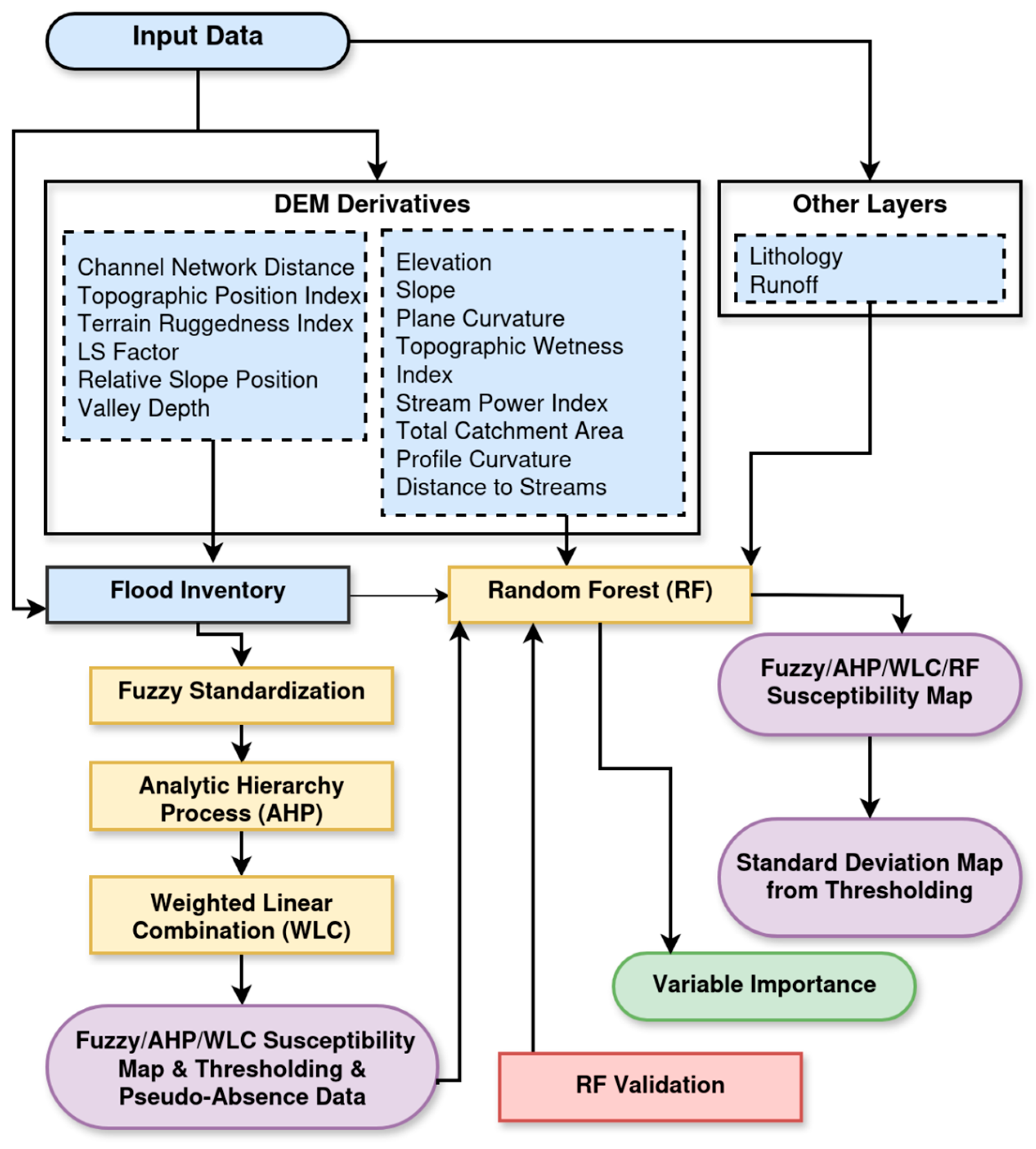
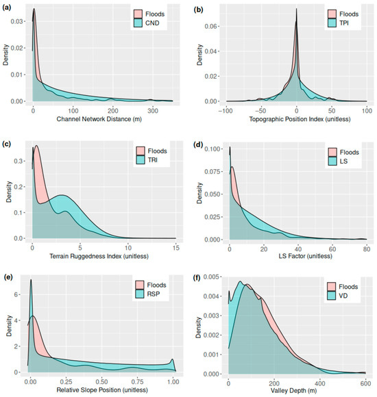
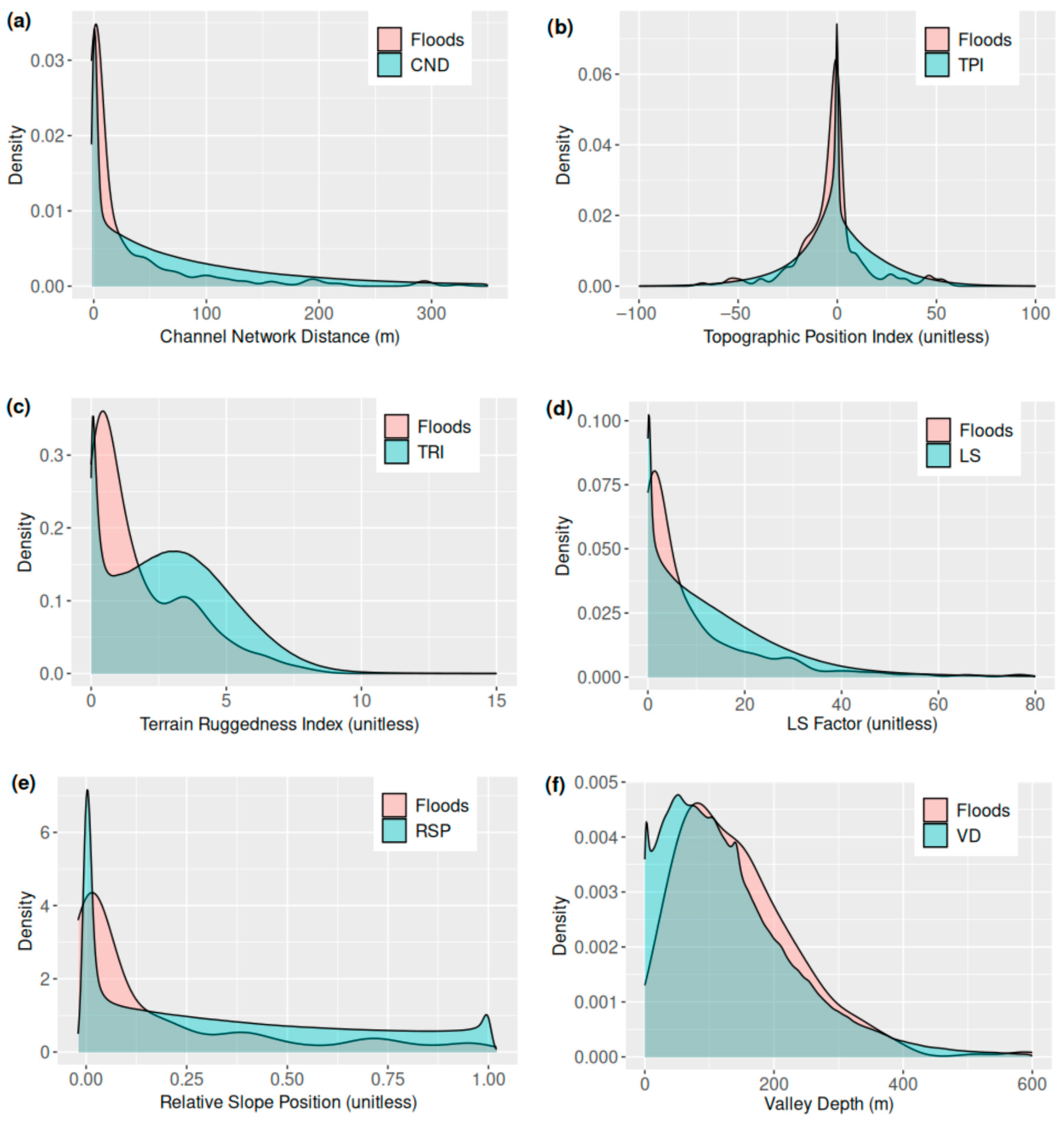
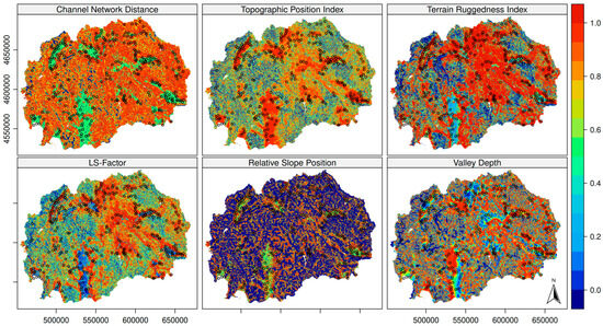
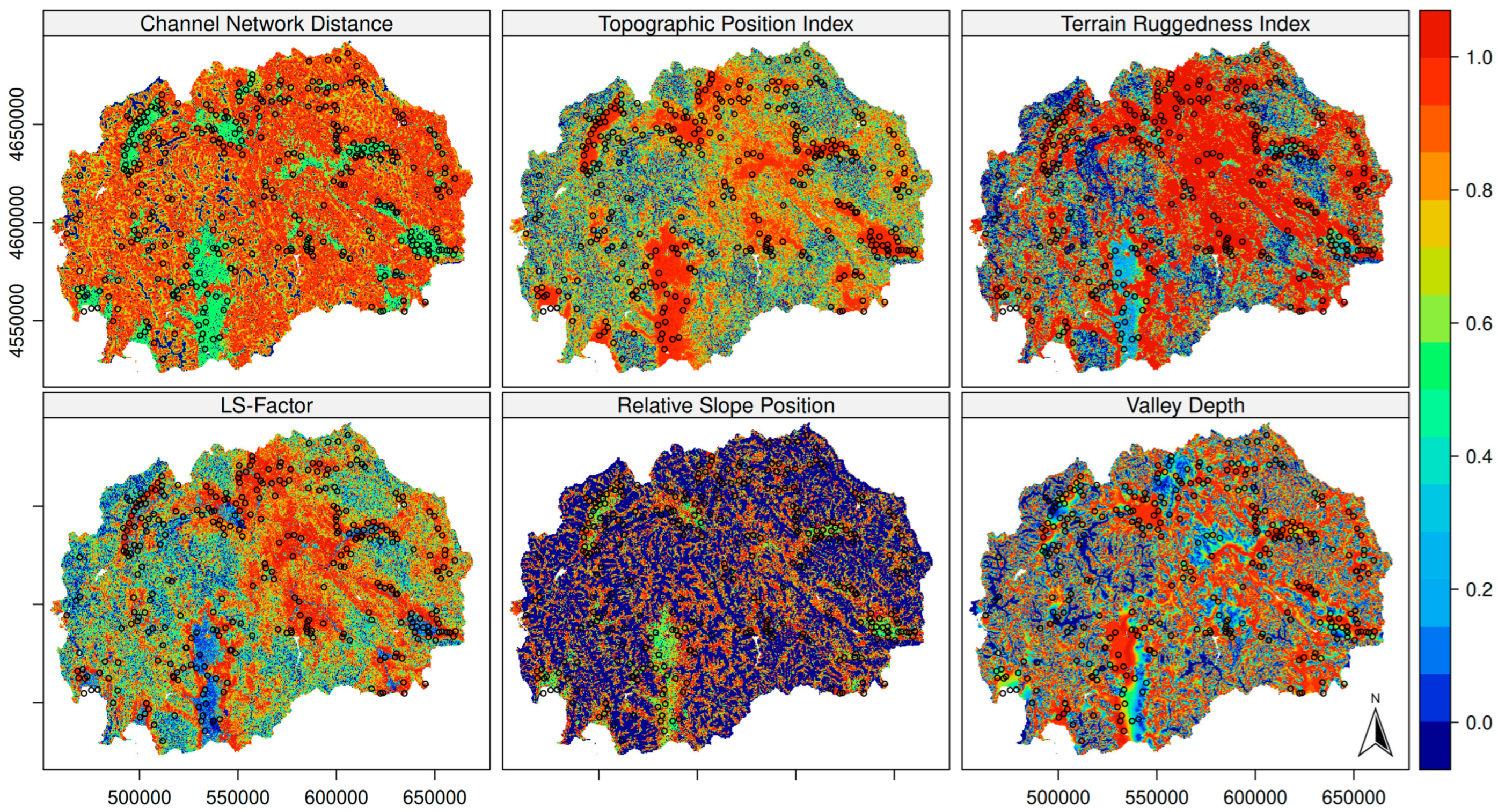
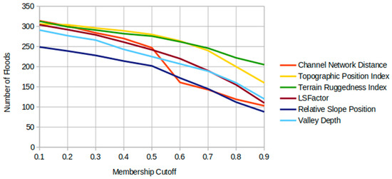
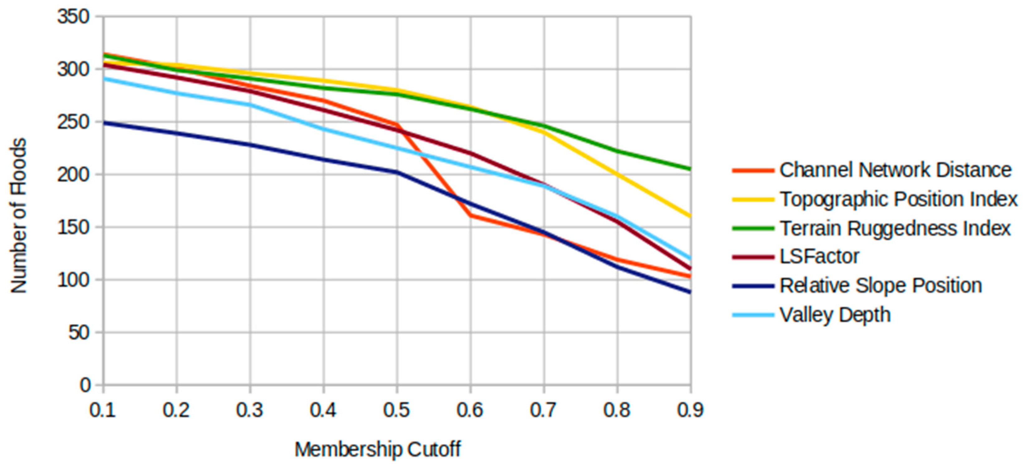
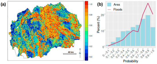
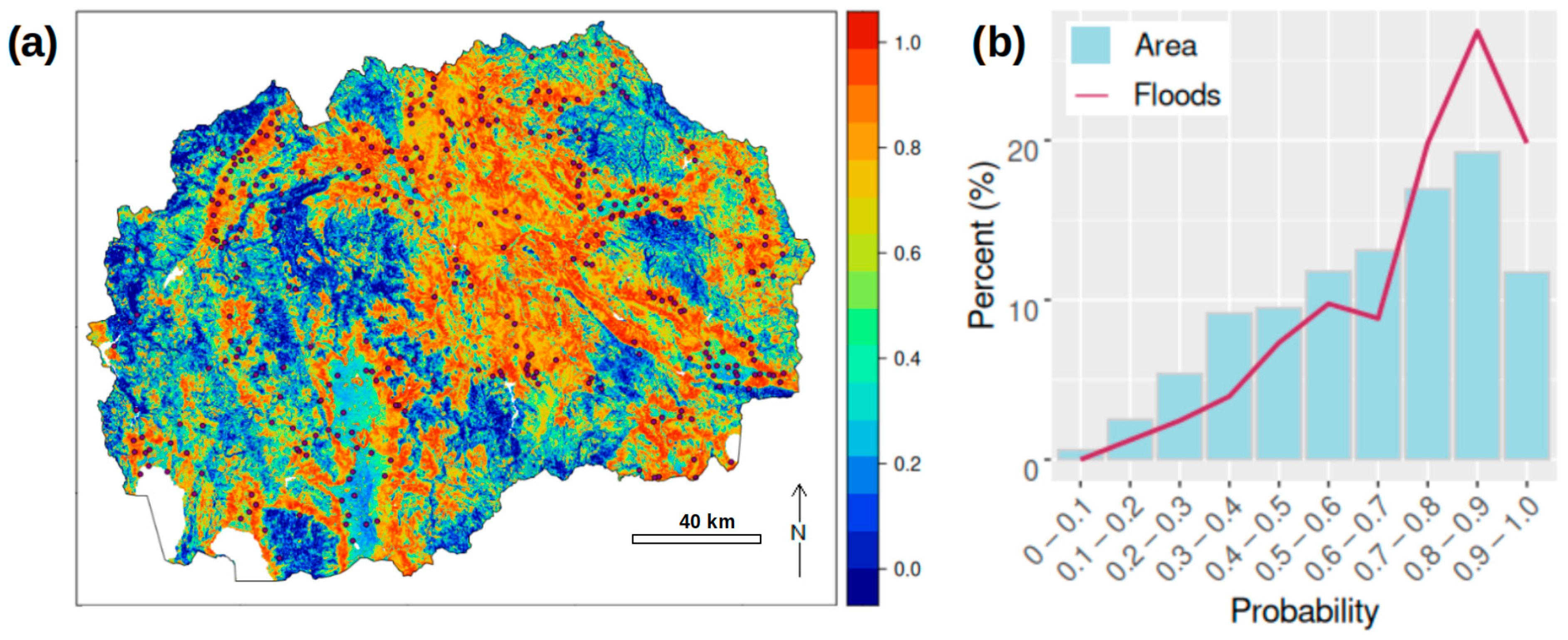
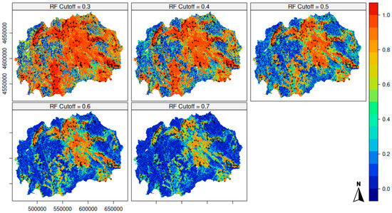
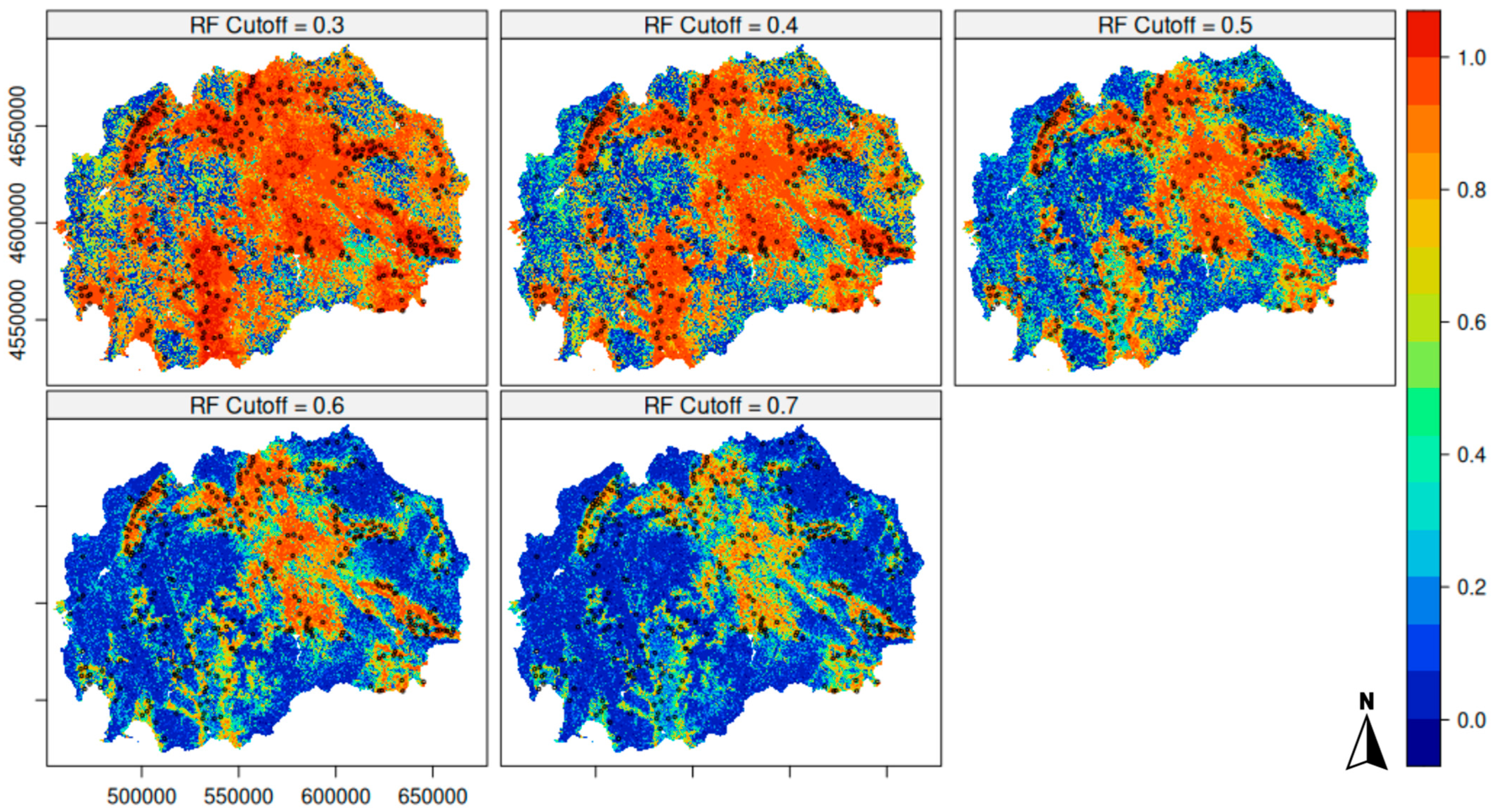
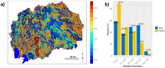
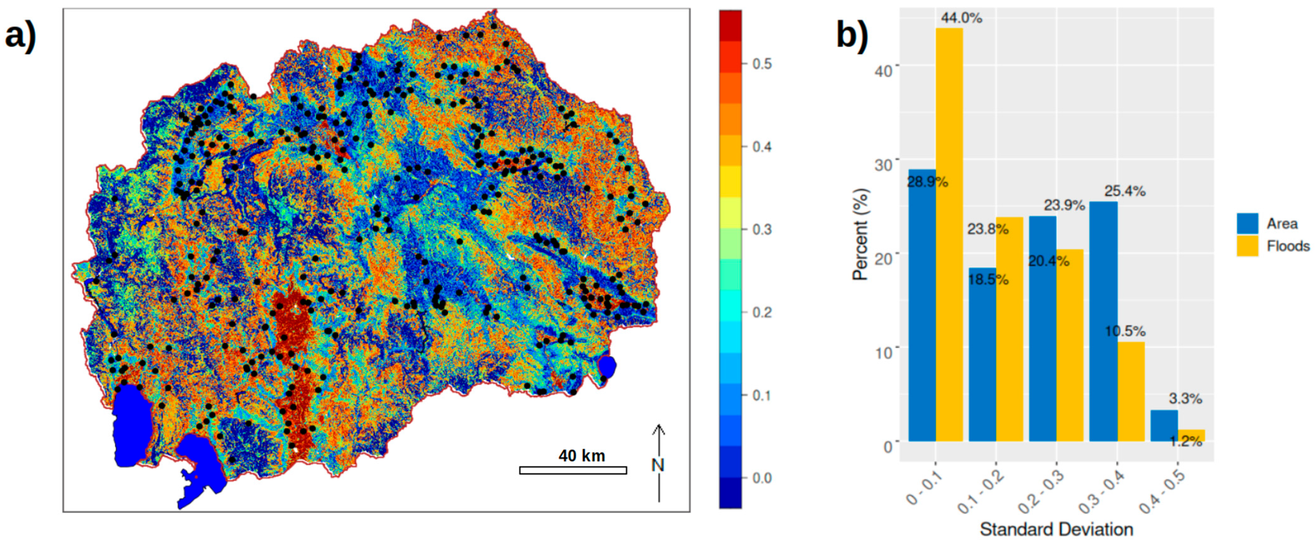
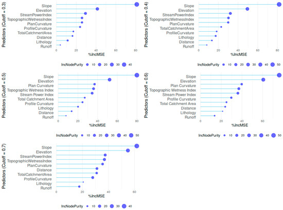
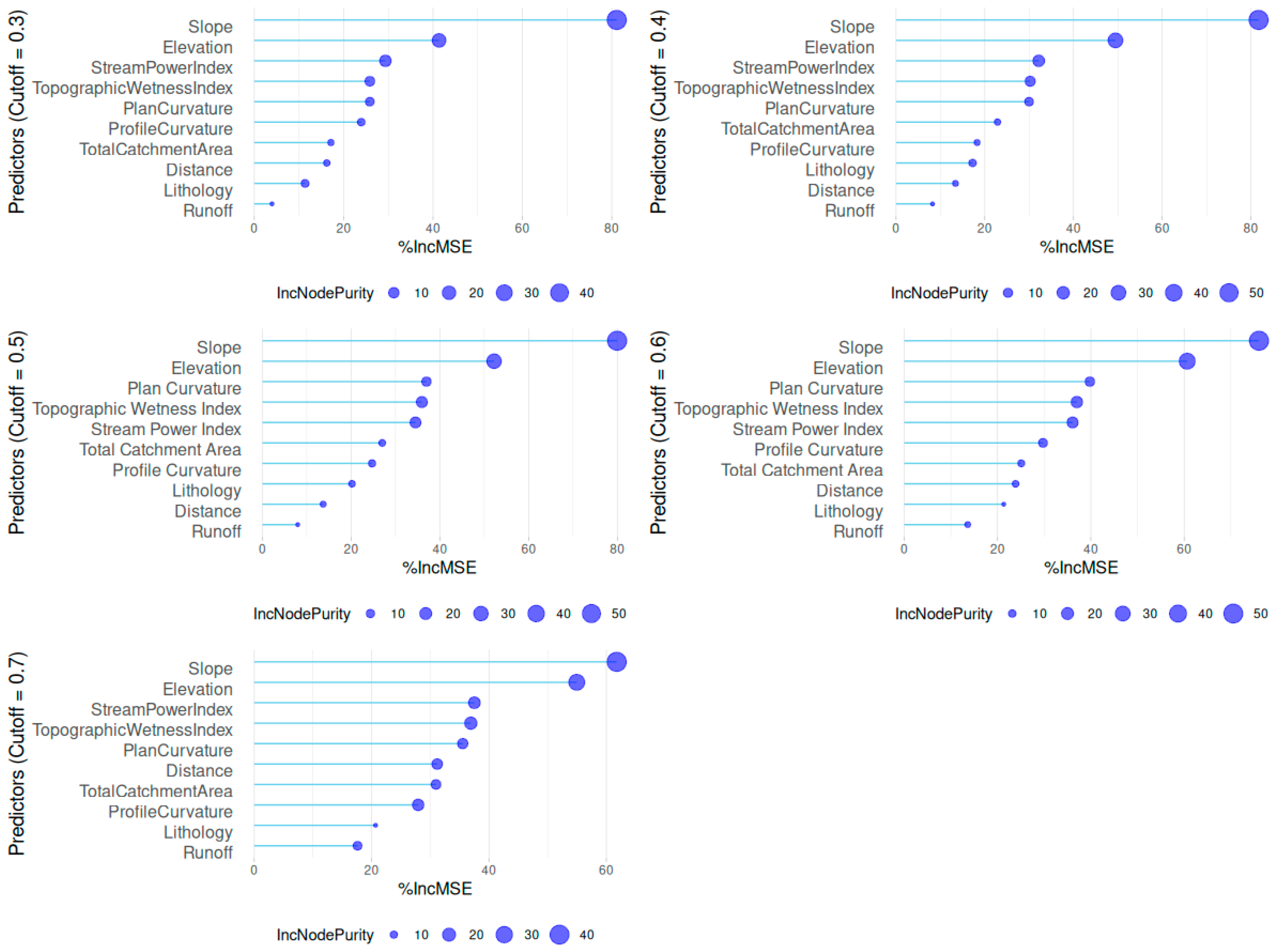
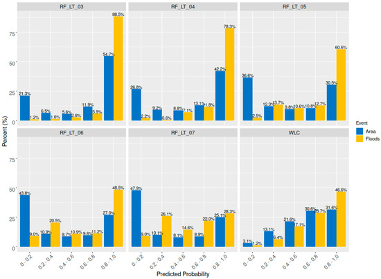
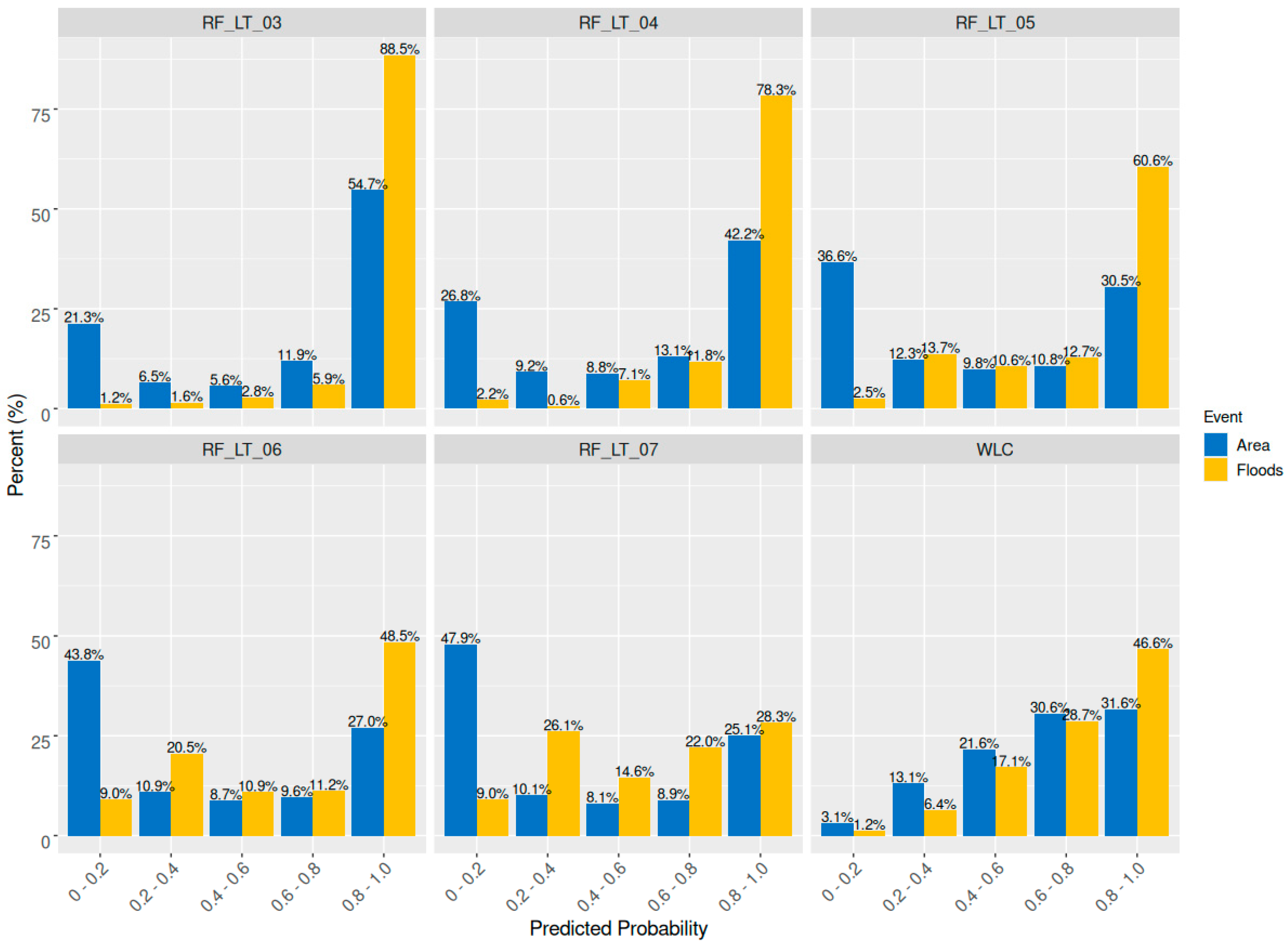
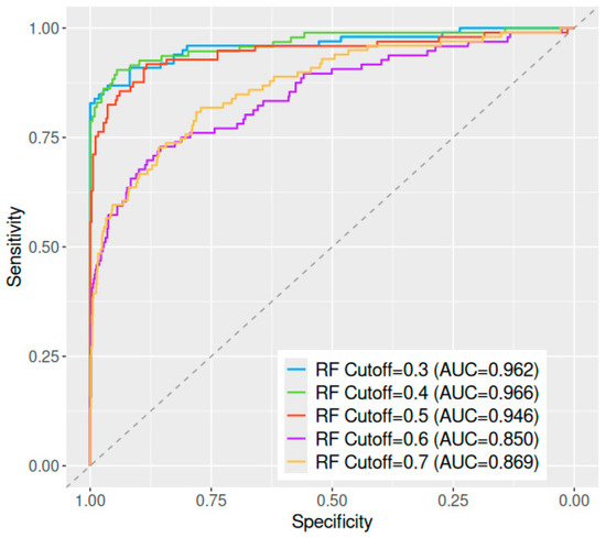
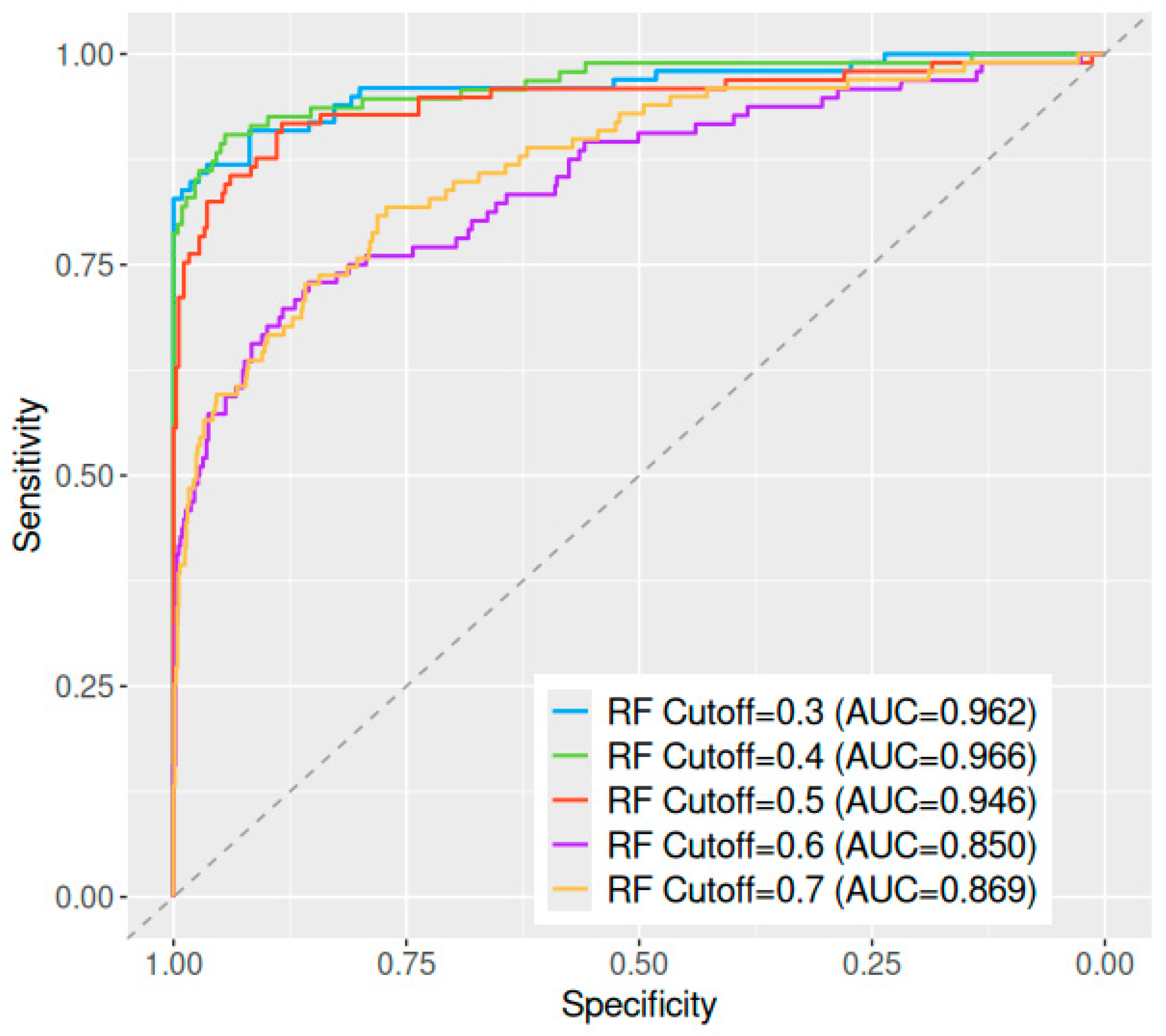

Disclaimer/Publisher’s Note: The statements, opinions and data contained in all publications are solely those of the individual author(s) and contributor(s) and not of MDPI and/or the editor(s). MDPI and/or the editor(s) disclaim responsibility for any injury to people or property resulting from any ideas, methods, instructions or products referred to in the content. |
© 2026 by the authors. Published by MDPI on behalf of the International Society for Photogrammetry and Remote Sensing. Licensee MDPI, Basel, Switzerland. This article is an open access article distributed under the terms and conditions of the Creative Commons Attribution (CC BY) license.