


Abstract
Does where an incident happens affect how quickly first responders arrive? Timely emergency responses are important to urban safety. However, the combined influence of street-level environments, operational conditions, and neighborhood contexts on dispatch performance remains unclear. We examined such geographical complexity by modeling geographic predictors for whether emergency vehicles successfully arrived at incidents in the city of Dallas within the city’s eight-minute benchmark. Using 250,647 incidents and 56 million GPS points along emergency dispatch routes in 2016, we compiled fourteen spatial and operational variables for every incident to train a Bayesian-optimized random forest classifier. The fourteen variables characterized street network topology, roadway attributes, land use, and socioeconomic status, and the model achieved an accuracy of 77.26% in predicting whether emergency response arrived at an incident within eight minutes. A longer distance to dispatch stations, dispatching from non-nearest stations, and low street–network integration were the strongest predictors of unsuccessful responses. Higher-income areas showed slightly elevated unsuccessful rates linked to frequent construction-related disruptions. These findings highlight emergency response as a coupled spatial–operational–temporal process and underscore the need for context-sensitive dispatch strategies and coordinated urban planning.
1. Introduction
Emergency response is a time-critical public service in which even modest delays can have life-threatening consequences. According to the National Emergency Medical Service (EMS) data, every minute of delay in prehospital care significantly decreases survival probabilities for cardiac arrest, traumatic injury, and other acute emergencies [1]. EMSs arriving within clinically recommended time windows can stabilize patients effectively, reduce morbidity, and improve long-term outcomes. Yet many constraints are present in an urban environment, such as narrow streets, irregular street grids, congestion, construction, and physical barriers, which impede emergency vehicle movement and contribute to avoidable delays. Understanding how these geographical conditions shape EMS performance at the incident level is, therefore, essential for developing context-sensitive dispatch strategies and enhancing urban resilience.
Emergency response time is typically defined as the interval between the receipt of an emergency call and the arrival of emergency vehicles at the scene [2]. Efforts to reduce response time have long constituted an important topic in EMS research. Some propose technological solutions. For example, Gao et al. (2024) [3] formulated a joint operation of uncrewed aerial vehicles (UAVs) and emergency medical services (EMSs) to improve timely response to opioid overdose cases. Yu et al. (2022) [4] reviewed traffic control strategies to reduce emergency vehicle travel time by developing rules or algorithms for route optimization, signal pre-emption, lane reservation, and hybrid strategies. While these technical solutions can be effective, the demand on operational coordination is high and may not be practical in all urban governance. Regarding route selection, Bandyopadhyay and Singh (2016) [5] found that 80% of dispatching routes taken by first responders at Allahabad Fire Station in Indian well matched routes predicted by Dijkstra’s shortest path algorithm on a road network weighted with road width, land use, and population density, variables which are static and lack operational considerations in terms of station distributions. Although routes chosen by first responders align with the algorithmic suggestions, shortest paths may not be the fastest options. Dynamic factors characterizing dispatch stations, neighborhoods or land use functions, weather conditions, and situations on the roads may hamper routing efficiency.
A substantial body of research has examined how area-based sociodemographic and geographic conditions influence emergency response at macro scales such as ZIP codes or census tracts [6,7,8]. Based on 4004 identified strokes in Nueces County, Texas, USA, [7] showed that the use of EMSs in stroke care varied from 17% to 71% across neighborhoods, and the adjusted EMS use for stroke was lower in neighborhoods with higher family income and a larger percentage of older adults. Although these studies have advanced important insights into broad neighborhood-level disparities, their reliance on aggregated areal units obscures spatial variation within these units and is vulnerable to ecological bias [9]. Individual-level emergency incidents may be influenced by highly localized barriers—such as micro-scale street geometry, distance to stations, or local traffic patterns—that cannot be observed at the zone level. Therefore, studies are needed to holistically include the influence of local environments on emergency response efficiency at the level of individual calls. This study directly addresses this gap by assessing how fine-scale geographical environments shape the likelihood of meeting the city-defined performance target for individual emergency calls.
Official performance assessment for emergency responses is commonly based on response time, even though patient outcomes [10] and quality of patient care [11] should be equally, if not more, important. Guidelines from the National Association of EMS Physicians recommend fractal performance metrics that classify responses based on whether they fall within pre-established thresholds [12]. These threshold-based metrics assess system performance with an emphasis on reliability and consistency. While the National Fire Protection Association (NFPA 1710) recommends a 9 min overall response target, the City of Dallas adopts a more stringent 8 min threshold—also commonly used in prior research [13,14,15]. Accordingly, this study evaluates individual incidents in terms of successful responses (≤8 min) and unsuccessful responses (>8 min).
Emergency response performance is shaped by several core determinants. At the most fundamental level, dispatch-related spatial dynamics—especially the distance between the incident and responding unit, as well as whether the nearest available station is the one dispatched—strongly influence the speed of response. Prior work has shown that greater separation from emergency facilities and higher workload at stations can contribute to longer response times [16]. These findings highlight the interaction of spatial configuration and operational burden as key drivers of service effectiveness across the urban landscape.
Traffic congestion further complicates the movement of emergency vehicles. Congestion can prevent drivers from clearing a path for EMS units, produce chokepoints, and magnify delays on high-volume corridors. Griffin & McGwin (2013) [17] found that congestion on interstate and major highways adds an average of 10 min to response times. Lee et al. (2018) [18] and Fu et al. (2022) [19] reported that crashes occurring on freeways and expressways generally cause longer response times compared to on collectors or local roads due to restricted access points and turning limitations. These studies suggest that certain road types inherently constrain incident access, making roadway classification an important contextual variable for incident-level analysis.
Although extensive research has shown that street–network configuration strongly shapes ordinary vehicular movement [20], congestion patterns [21], and route selection [22], its influence on emergency mobility remains comparatively underexamined in EMS research. Space syntax provides a robust theoretical and analytical lens for understanding how the structural configuration of street networks shapes movement, accessibility, and route choice. Two measures are especially relevant: integration and choice. Integration captures how accessible a street segment is to all other segments in the network and is measured by the number of directional changes required to travel to all other points [23]. Streets requiring fewer turns to reach everywhere in a network exhibit higher integration and tend to occupy locations closer to the central position in the network, whereas streets with low integration values tend to be more isolated [24]. Choice measures the extent to which a given street segment lies on the shortest paths between all origin–destination pairs, serving as a proxy for through-movement potential [25,26]. Together, integration and choice capture key topological properties of street networks that influence movement flows. Incorporating these measures into incident-level analysis allows us to examine how variations in network configuration shape emergency vehicle accessibility and response outcomes within the urban street system.
Beyond network structure, socioeconomic environments form another critical layer in understanding disparities in emergency response performance. Socioeconomic status (SES) is widely used as a proxy for resource access, exposure to risk and cumulative disadvantage across health [27], economic, and urban geographic domains [28]. Empirical studies reveal that low-income areas experienced longer EMS responses than high-income neighborhoods, and higher income zip codes statistically have a higher likelihood of EMS responses in 8 min [6]. Similarly, statistics based on the Greater Cincinnati/North Kentucky Stroke Study suggested EMS calls for acute stroke from households living below the poverty line could be up to 5 min longer than the average EMS responses [29]. These findings suggest that socioeconomic disadvantage can intersect with spatial and operational factors to produce uneven geographies of emergency response, warranting a more granular, incident-level assessment.
Given these conceptual foundations, researchers have applied various statistical approaches to model emergency response times and identify significant predictors of delay. In such models, researchers typically define a dependent variable (), most commonly the Total Response Time (continuous) or Patient Survival Status (binary), and regress it against a vector of explanatory variables () such as travel distance, temporal factors (hour of day, day of week), weather conditions, and operational constraints (crew turnout time). While traditional approaches utilize Multivariate Linear Regression (OLS) [30] or Logistic Regression [31] to estimate these relationships, modern methodologies have increasingly shifted toward Machine Learning (ML) techniques. These advanced methods, particularly ensemble learning algorithms, are employed to capture the complex, nonlinear interactions between the built environment and service performance that classical statistical models often fail to identify (e.g., the compounding effect of rain during rush hour versus rain at midnight).
To address the limitations of traditional statistics models and to capture potentially nonlinear interactions among built-environment, socioeconomic, and operational predictors, this study employs classification-based modeling. While logistic regression is a common tool for binary outcomes, its assumptions regarding linearity in log-odds, additivity, and limited interactions constrain its ability to represent complex urban processes. Urban emergency response is shaped by multidimensional, interdependent factors—including street topology, station availability, roadway classification, congestion, and SES—that likely exhibit nonlinear and hierarchical interactions. A more flexible modeling approach is therefore required to identify the key geographical predictors that influence whether emergency dispatches meet the performance threshold.
This study adopts a machine learning classification framework—implemented through random forest modeling—to evaluate incident-level emergency response performance in the City of Dallas, Texas. Random forests allow for the incorporation of complex interactions, spatial heterogeneity, and nonlinear relationships without imposing strict parametric assumptions [32]. While logistic regression considers one model for all incidents, random forests include multiple regression trees, each of which consists of randomly selected features (i.e., explanatory variables) across a hierarchy of decision branches. The prediction of the emergency response for each incident is a collective decision across all trees. As such, random forests can consider diverse factors and their mechanisms that influence emergency response performance across different geographic contexts. Importantly, the goal in this study is not only prediction but also explanation: identifying which built-environment, socioeconomic, and operational variables most strongly shape the likelihood of a successful response. Consequently, this paper utilizes the random forest model to examine the relationship between geographical features and emergency dispatch at the incident level.
In general, this study makes three contributions to research on urban accessibility and emergency service provision. First, it advances existing work by moving from area-based analyses to an incident-level, fine-scale examination of intra-urban spatial variation in emergency response performance, thereby reducing aggregation bias and revealing localized accessibility constraints that are invisible in zonal studies. Second, it introduces street–network configuration measures, specifically integration and choice, to the analysis of emergency response, demonstrating that network topology and urban morphological structure shape response outcomes in ways that cannot be captured by distance or road classification alone. Third, from a methodological perspective, the study employs a classification-based modeling framework to identify and interpret these relationships, but the primary contribution lies in clarifying how urban spatial structure, network accessibility, and land use context jointly shape the outcome of emergency response within the city.
The remainder of this paper is structured as follows. The Materials and Methods Section describes the technical details of hyperparameter selection, optimization, and model training. The Results Section presents the model’s performance in predicting emergency responses at the individual level and evaluates the importance and contributions of the top-ranked geographical features. Finally, the Conclusions Section summarizes the key findings, discusses the study’s limitations, and outlines directions for future research.
2. Materials and Methods
2.1. Study Area and Trajectories Based on Global Positioning System (GPS) Data
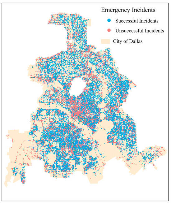
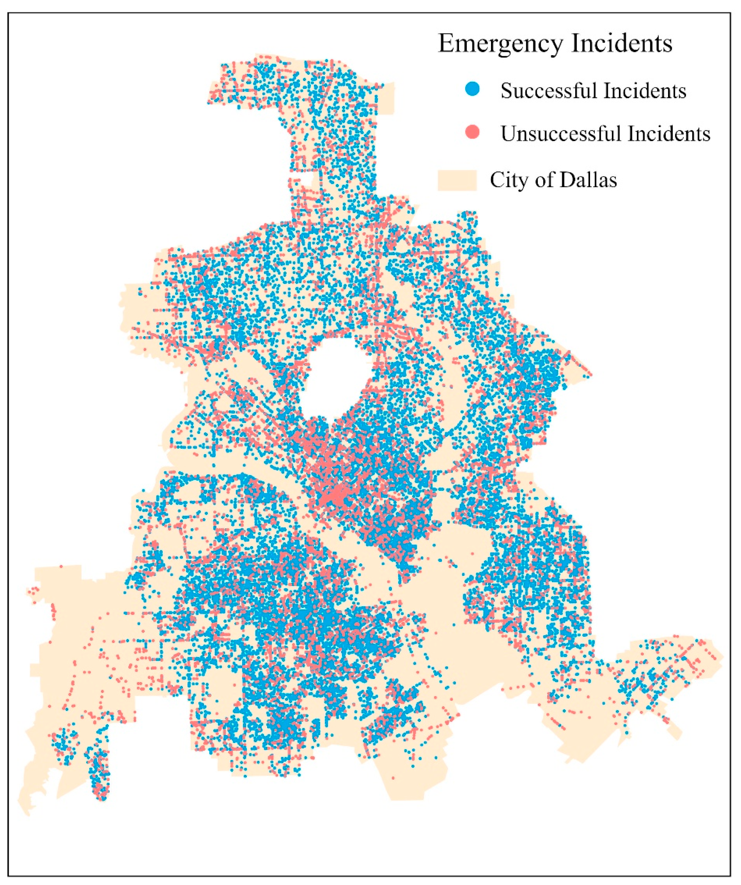
This study acquired 250,647 Dallas emergency incidents from January to December 2016 and corresponding GPS trajectories of Emergency Vehicle (EV) dispatches with a total of 56,185,419 GPS points from the Dallas Fire and Rescue stations across the city. Figure 1 shows the spatial distribution of emergency incidents across the city of Dallas during the study period. The University Park, depicted as the central void in Figure 1, operates under a different fire -rescue department system. Consequently, this study opted to exclude University Park from the study area.
Figure 1.
Spatial distribution of emergency incidents in Dallas, Texas, in 2016. Blue points represent successful emergency dispatches, while red points indicate unsuccessful incidents. The background polygon shows the boundary of the City of Dallas.
The study’s unit of analysis is an emergency vehicle run (henceforth, a run, for simplicity) when an EV responds to the received emergency call to elicit geographic factors that influence individual runs. Meanwhile, EMS performance is evaluated at the level of incidents. The Computer-Aided Dispatch (CAD) system used by the city of Dallas sends multiple EVs (hence, multiple runs) to a received emergency call to maximize the likelihood of a timely response. A successful run means that an EV arrives at the location of the emergency incident within eight minutes of receiving that emergency call, as the standard in the city of Dallas. An emergency response to an incident is considered successful as long as one EV has arrived at the assigned incident location within eight minutes; otherwise, it is considered an unsuccessful response to the incident.
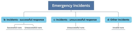
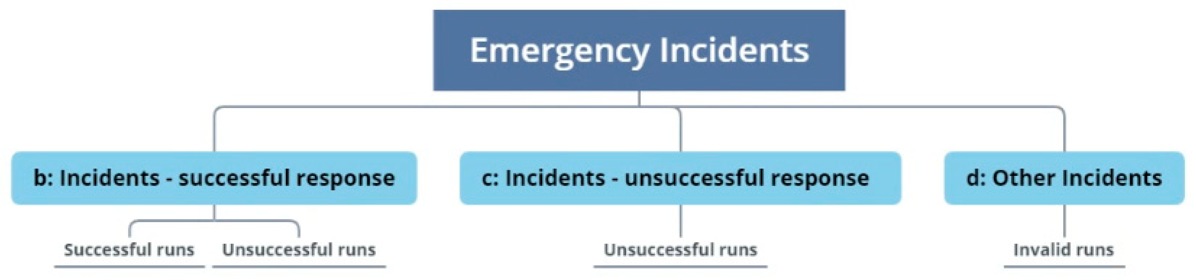
Incident locations were based on geocoded addresses or call detailed record (CDR) estimates, while EV locations came from onboard GPS devices. To account for location uncertainty, this study assumed a distance threshold of 150 m to the call site for arrival determination. Hence, a run would be successful when an EV arrived within 150 m of an incident location in 8 min or less. For example, a run is labeled as successful (class = 1 in the random forest model) if an emergency vehicle’s GPS position enters the 150 m buffer around the incident location within 8 min. Response time is computed as the interval between the first GPS record following dispatch and the first GPS point located within the 150 m buffer. Based on the distance and time thresholds, all 250,647 Dallas emergency incidents from January to December 2016 were characterized into three categories: incidents with successful responses, incidents with unsuccessful responses, and other incidents (Figure 2). Other incidents had no EVs arriving within the distance thresholds due to the utilization of alternative resources or cancelations. Table 1 lists the number of incidents in each category. The success rate is the proportion of incidents with successful responses out of the total of incidents with successful responses and incidents with unsuccessful responses ().
Figure 2.
Classification of emergency incidents based on emergency response outcomes. Incidents are categorized into three groups: (b) incidents with successful responses, including both successful and unsuccessful runs; (c) incidents with unsuccessful responses; and (d) other incidents, including invalid runs.
Table 1.
Incidents categorized by emergency responses.
2.2. Geographical Variables
This study employed fourteen variables representing different categories to describe the geographical environments of emergency dispatch (Table 2) based on prior studies, as discussed in the Introduction Section. American Community Survey (ACS) data at the census tract level contain rich socioeconomic metrics and have been used extensively to characterize socioeconomic status at the neighborhood level. This study retrieved median household income and the percentage of households below 200% of the Federal poverty level to characterize the neighborhood’s economic status. To characterize road attributes at emergency incident sites, this study downloaded Dallas’ Road from the Texas Department of Transportation (TxDOT) with road type and lane count.
Table 2.
Explanatory variables to classify incidents with successful or unsuccessful responses.
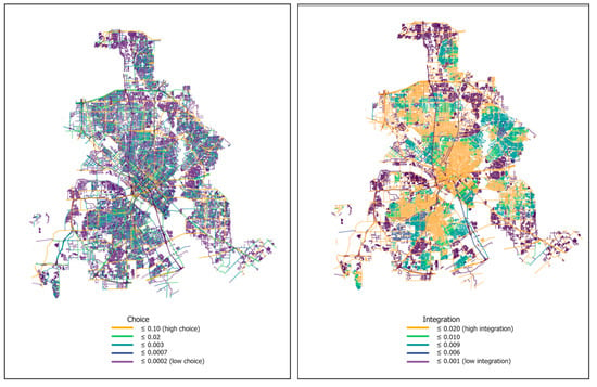
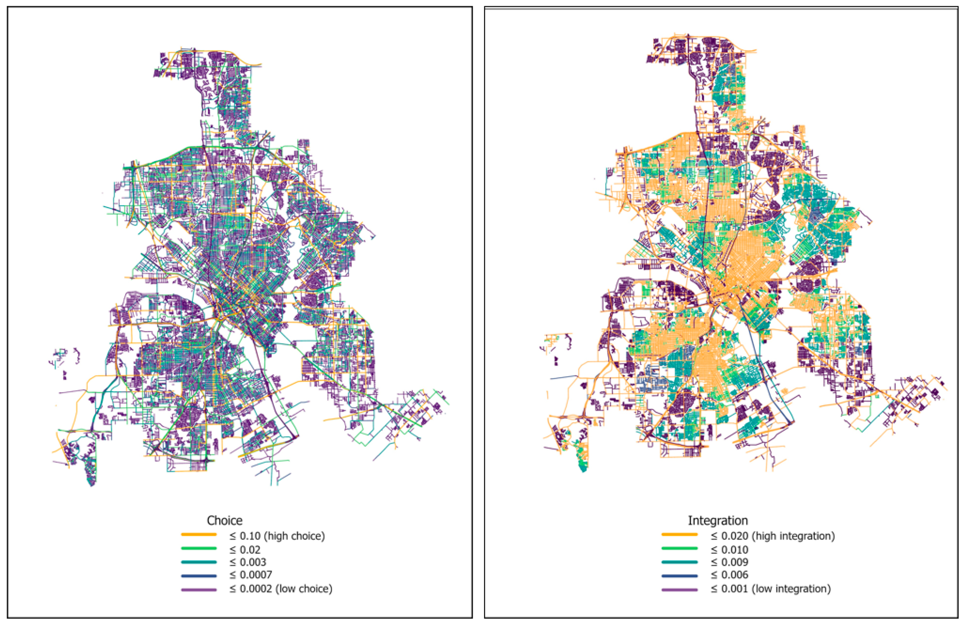
Choice and Integration quantify the positioning of each street segment and their relationships in the road network to evaluate the accessibility of a street segment. These measures were calculated using angular segment analysis. Choice reflects how often a street segment is likely to be part of the shortest routes between different locations in the network. Integration indicates how close a street segment is to all other segments in terms of travel through the network. Higher values of choice or integration therefore represent streets that are more central in the network and more accessible compared to other street segments. In Figure 3, street segments with higher choice values correspond to highways and major roads, indicating that highways and major roads are more likely to be part of the shortest paths between different origins and destinations in the road network. Street segments with higher integration correspond to those located in the central parts of the network or in regions near highways, because they have shorter overall topological distances to other segments and therefore provide higher accessibility within the street network.
Figure 3.
Spatial distribution of street network choice (left) and integration (right) derived from angular segment analysis. Higher values (yellow) indicate street segments that are more likely to be part of shortest paths (choice) or more centrally accessible within the network (integration), while lower values (purple) represent more peripheral streets.
All explanatory variables related to socioeconomic conditions, site characteristics, and street topology were extracted based on the location of each emergency incident. For the categorical explanatory variables, they were encoded using one-hot encoding prior to model training.
The dispatch operation encompassed attributes associated with both the Fire Rescue Department and its emergency vehicles. Key operational variables included the annual call volume, defined as the total number of emergency incidents reported to a department within a calendar year, and the total number of runs (i.e., the number of dispatched emergency vehicles) per incident. Network distance was calculated based on the street network following [33]. This street network contained lines and points, where lines were also called edges (representing a street segment) and points were the same as nodes (representing the endpoints of a street segment). Each edge has two pieces of information, denoted as ‘from’ and ‘to’ nodes of the edge’s endpoints. For example, an edge (representing a street segment) with ‘from’ equal to 1 and ‘to’ equal to 2 indicates the traffic direction from node 1 to node 2. Based on the GPS trajectories of emergency dispatch vehicles, we extracted the street segments traversed during each response. The total network distance was then calculated by summing the lengths of all traversed street segments.
The variable “nearest Fire Rescue Department” indicates whether an emergency vehicle is dispatched from the nearest Fire Rescue department (DFR), denoted by a binary response of ‘yes’ or ‘no’. Explanatory variables related to dispatch operations were derived from the station from which the emergency vehicle was dispatched
Land use data from the North Central Texas Council of Governments (NCTCOG) Regional Data Center Site (https://data-nctcoggis.hub.arcgis.com/), accessed on 1 March 2020. provided the land use classes at incident locations. The NCTCOG regional government provides detailed metadata documentation for the land use dataset at their data portal to ensure data validity for research applications. Rather than treating land use as a purely descriptive variable, this study uses land use type as a proxy for differences in locational specificity and site accessibility. Locations in single-family residential areas typically have well-defined street addresses and clearly marked access points, whereas incidents occurring in large open spaces, industrial parcels, campuses, or transportation facilities often involve greater locational ambiguity and more complex internal access conditions. Such differences can affect the time required for emergency vehicles not only to reach the vicinity of an incident, but also to identify and access the precise location within a site. Land use context, therefore, captures an important dimension of micro-scale accessibility that is not represented by street network distance alone. Temporal variables (hour of day and day of week) were included to capture systematic diurnal and weekly variation in traffic conditions and travel time reliability. In urban transportation systems, traffic volume and congestion levels follow strong and repeatable temporal rhythms, with pronounced differences between peak and off-peak periods and between weekdays and weekends. Accordingly, time-of-day and day-of-week indicators are widely used in transportation [34] and emergency service studies as proxies for temporal variation in congestion intensity and network performance. In this study, these variables serve to represent the temporal structure of urban mobility conditions and are defined based on the time at which the incident occurred. The original incident types provided for each emergency call were reclassified into Lower Priority, Higher Priority, and Highest Priority based on the guidelines outlined in the National Fire Protection Association (NFPA) Standard 1710 (https://fems.dc.gov/page/evaluating-call-volume), accessed on 1 April 2020.
2.3. Random Forest Model
The random forest (RF) classification model was used to predict whether an emergency incident achieved a successful response (coded as 1) or an unsuccessful response (coded as 0). Fourteen predictor variables capturing temporal characteristics, site and built-environment features, dispatch operations, street–network topology, socioeconomic conditions, and urban environmental contexts were included as covariates. A total of 250,641 emergency incidents in 2016 served as the modeling dataset.
To train and evaluate the RF model, the dataset was randomly partitioned into 70% training (164,788 incidents) and 30% testing (70,623 incidents) subsets using stratified sampling to preserve the original class distribution across the study area. To ensure that model performance was not sensitive to any particular random partition, this procedure was repeated 20 times using different random splits, and the resulting performance metrics showed negligible variation. Model performance was assessed using sensitivity, specificity, and overall accuracy, metrics commonly used in classification-based EMS and health service modeling. The sensitivity measures the proportion of successful responses (positive class) correctly identified by the model. The specificity measures the proportion of unsuccessful responses (negative class) correctly classified. The accuracy reflects the share of all incidents—successful and unsuccessful—predicted correctly. These three metrics jointly provide a comprehensive evaluation of the RF model’s ability to classify emergency response outcomes, particularly in the presence of imbalanced data.
2.4. Hyperparameter Tuning Using Bayesian Optimization (BO) in Hyperopt
Hyperparameter tuning was conducted using Bayesian Optimization (BO) implemented through the Hyperopt Python library, which identifies the optimal parameter configuration for the RF model. The BO procedure consists of four main stages: (1) defining the hyperparameter search space, (2) approximating the objective function using surrogate models, (3) selecting the next candidate parameters using an acquisition function, and (4) iteratively updating the surrogate model to converge on optimal values.
2.4.1. Phase 1: Defining the Hyperparameter Space
The hyperparameter search space specified the allowable ranges for parameters to be optimized. Five RF hyperparameters were tuned: (1) mtry: the number of variables randomly selected at each split; (2) max_depth: the maximum tree depth; (3) min_samples_split: the minimum number of observations required to split a node; (4) min_samples_leaf: the minimum number of observations required in each leaf; (5) n_estimators: the total number of trees in the forest. These parameters jointly control model complexity, tree diversity, and predictive stability.
2.4.2. Phase 2: Surrogate Modeling of the Objective Function
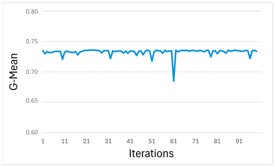
BO employs a surrogate model to approximate the objective function and efficiently navigate the hyperparameter space. As shown in Table 1, 205,242 (or 87%) of all incidents received EMS responses in 8 min or sooner. The data, therefore, were imbalanced towards successful responses. The G-Mean, balancing sensitivity and specificity ), was selected to serve as the objective function for imbalanced classification. The surrogate was trained on a subset of sampled configurations to estimate both expected G-Mean and its uncertainty across the search space. Each configuration was assessed via five-fold cross-validation, with models trained on 70% and tested on 30% of the data. The average G-Mean across folds informed the surrogate, enhancing stability and reducing bias and variance in performance estimation.
2.4.3. Phase 3: Acquisition Function for Guided Search
The acquisition function determines which hyperparameter set to evaluate next. The function guides BO toward regions of the search space likely to improve the objective function based on the surrogate model’s predictions and uncertainty levels. Regions with greater predicted improvement in G-Mean received priority for sampling, so that the acquisition function enabled BO to focus computational resources on promising areas rather than exhaustively searching the entire space.
2.4.4. Phase 4: Iterative Updating and Convergence
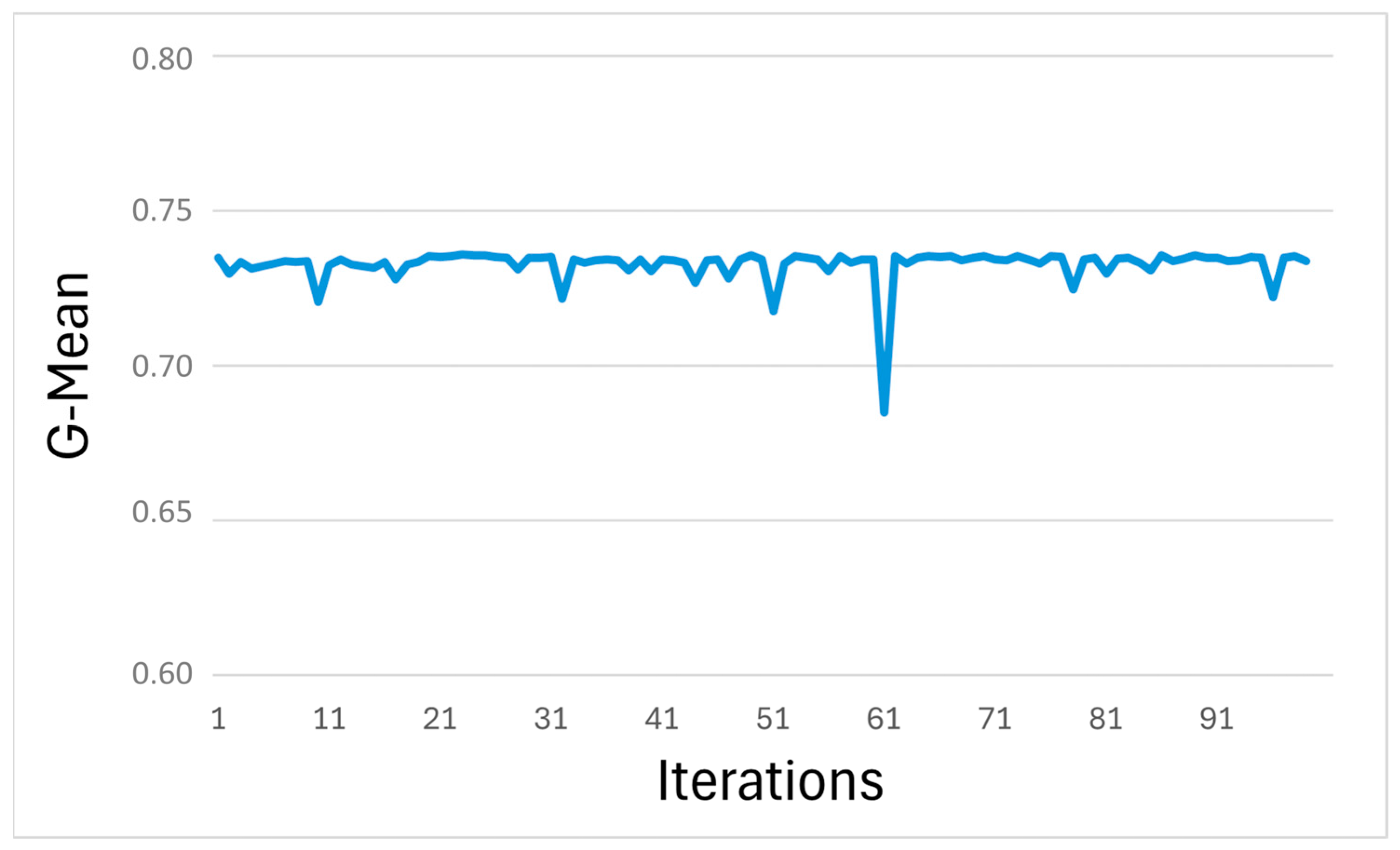
As new hyperparameter evaluations were completed, the surrogate model was updated to better its approximation of the objective function. This iterative process continued until a stopping rule was reached—in this case, 100 iterations. The BO process returned a set of hyperparameter–G-Mean combinations, revealing performance variation across the search space. As shown in Figure 4, G-Mean values ranged from 0.684 to 0.735 across sampled configurations. The highest G-Mean was obtained at iteration 34, representing the optimal balance between sensitivity and specificity. The final tuned hyperparameters were as follows: (1) mtry = 10; (2) max_depth = 41; (3) min_samples_leaf = 11; (4) min_samples_split = 295; (5) n_estimators = 1190. These values produced the best-performing RF model and were used for subsequent analysis and variable-importance assessment.
Figure 4.
Random forest hyperparameter optimization based on the G-mean metric. The horizontal axis represents the iteration number during the hyperparameter search, and the vertical axis shows the corresponding G-mean values.
2.5. Evaluation of Variable Importance Using Shapley Additive Explanations (SHAP)
The proposed RF model was evaluated for mode interpretability to (1) decipher the relationships between input variables and model predictions and (2) assess variables importance in driving the prediction. Lundberg and Lee (2017) [35] developed the Shapley Additive Explanations (SHAP) method to improve the interpretability by computing the SHAP values for each variable input to a model and provided insights into both the direction and magnitude of each variable’s influence on model predictions. A higher positive SHAP value signifies that the variable tends to push the predicted outcome further toward the positive class (i.e., successful responses) compared to a lower positive value. Conversely, a higher negative SHAP value indicates a stronger tendency for the variable to push the predicted outcome towards the negative class (i.e., unsuccessful responses) compared to a lower negative value.
The SHAP value for variable is determined through the weight of all marginal contributions using Equation (1):
where is a subset containing all variables excluding variable . Moreover, is the total number of variables, is the model’s prediction when considering both variables in subset and , and is the model’s prediction when only considering the subset .
The term in this equation is a weight factor to account for the size of subset and the total number of variables available. The difference between and quantifies the marginal contribution of variable to the model’s prediction.
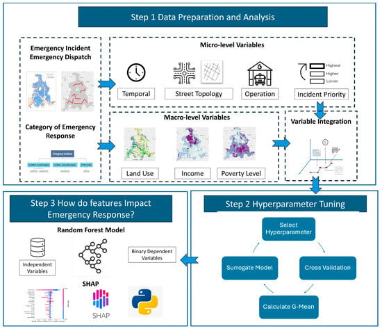
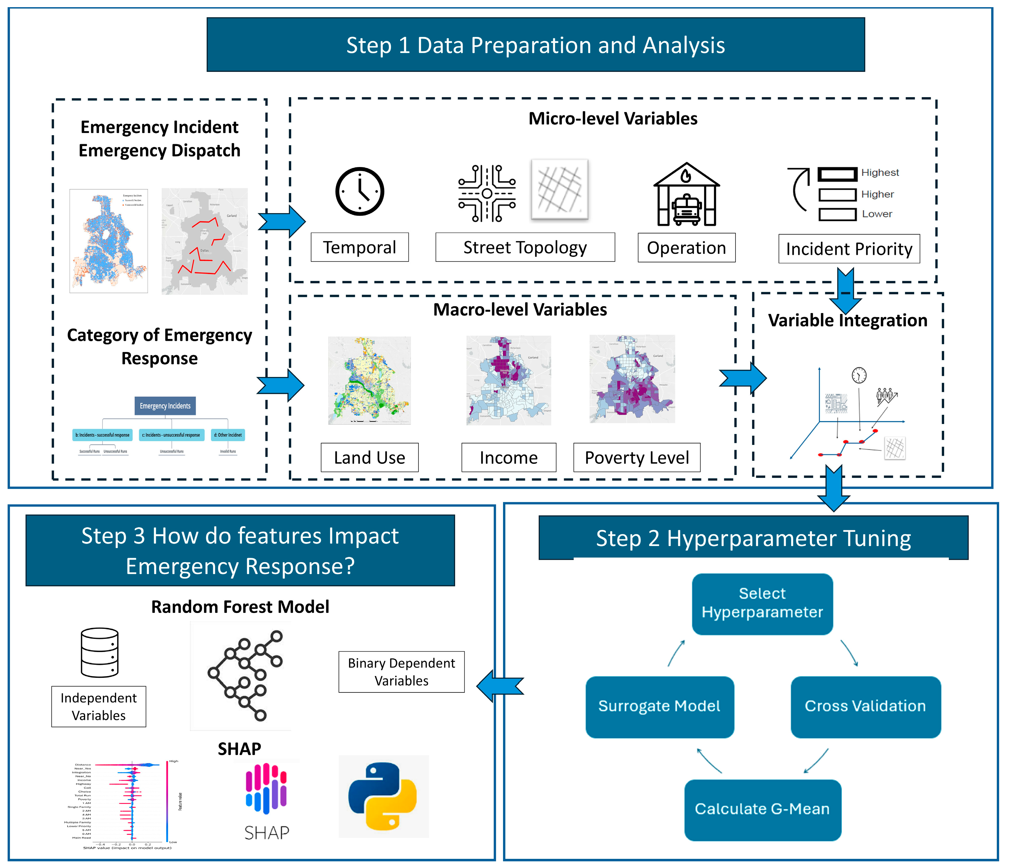
Overall, this study adopts this structured framework (Figure 5) to examine how geographical features shape emergency response performance. First, emergency incidents are classified into successful and unsuccessful responses, and a suite of micro- and macro-level variables are integrated at the incident level to enrich the geographic context along each dispatch route. The data preparation and analysis processes described in Step 1 were performed using R (4.0.0) and Python (3.8.2). Second, Hyperopt in Python elicited the optimal hyperparameters to obtain the best-performing Random Forest model. Finally, we quantified the contribution of each geographical variable to response outcomes for a detailed assessment of their relative influence.
Figure 5.
Research Framework for Modeling Emergency Response Performance.
3. Results
3.1. Random Forest Model Performance
This study examined the relationships between binary emergency response (successful vs. unsuccessful) and geographical variables by developing a random forest model. With the BO-based hyperparameter optimization, the model constructed a total of 1190 trees. For each tree, the modeling process randomly selected 10 variables for a node to separate incidents into two classes: incidents with successful responses (class = 1) or incidents with unsuccessful responses (class = 0). To mitigate overfitting, this study employed three different parameters to control tree size and depth: a maximum depth of 41, a minimum number of split leaves of 11, and a minimum number of split nodes of 295. As mentioned earlier, this study allocated 70% of the data for training and retained 30% for testing.
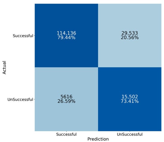
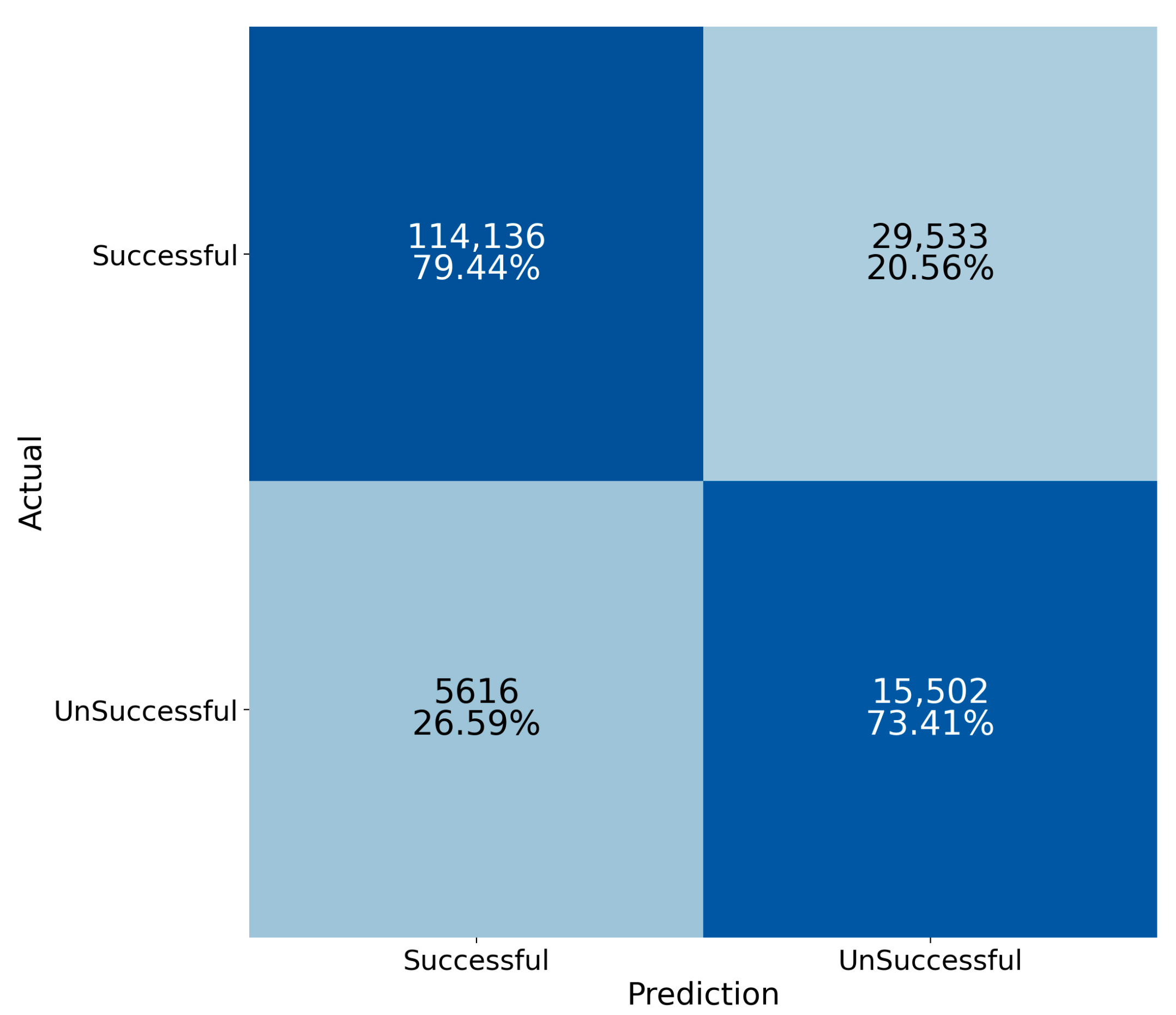
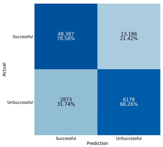
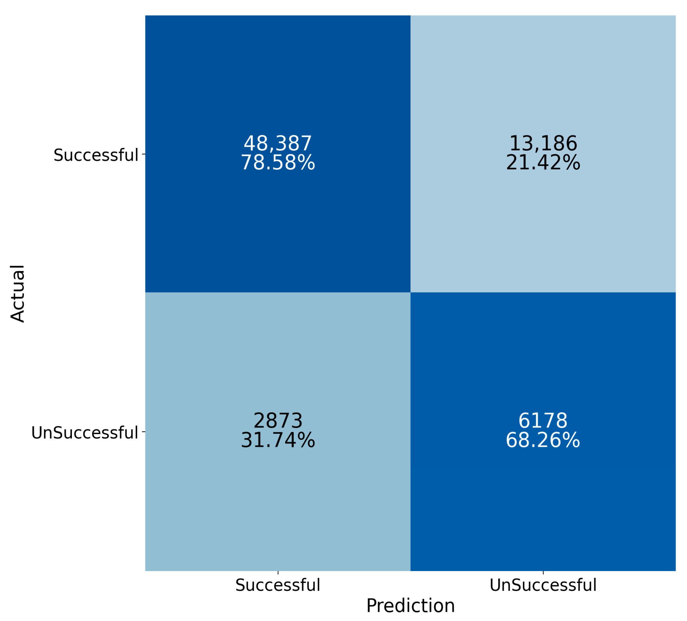
The specificity and sensitivity were illustrated in a 2 × 2 confusion matrix, delineating different classification scenarios for the samples. The confusion matrix for training and testing data showed comparable results, indicating that the model did not overfit the training data (Figure 6 and Figure 7). With the training data, the random forest model correctly predicted 79.44% of emergency incidents in the successful group and 73.41% of emergency incidents in the unsuccessful group. The overall accuracy was 78.67%. Subsequently, when applied to unseen testing data, the model correctly predicted 78.58% of emergency incidents in the successful group and 68.26% of emergency incidents in the unsuccessful group. The overall accuracy was 77.26%.
Figure 6.
A confusion matrix showing the classification performance of the random forest model on the training data.
Figure 7.
A confusion matrix showing the classification performance of the random forest model on the testing data.
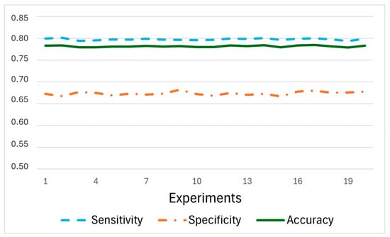
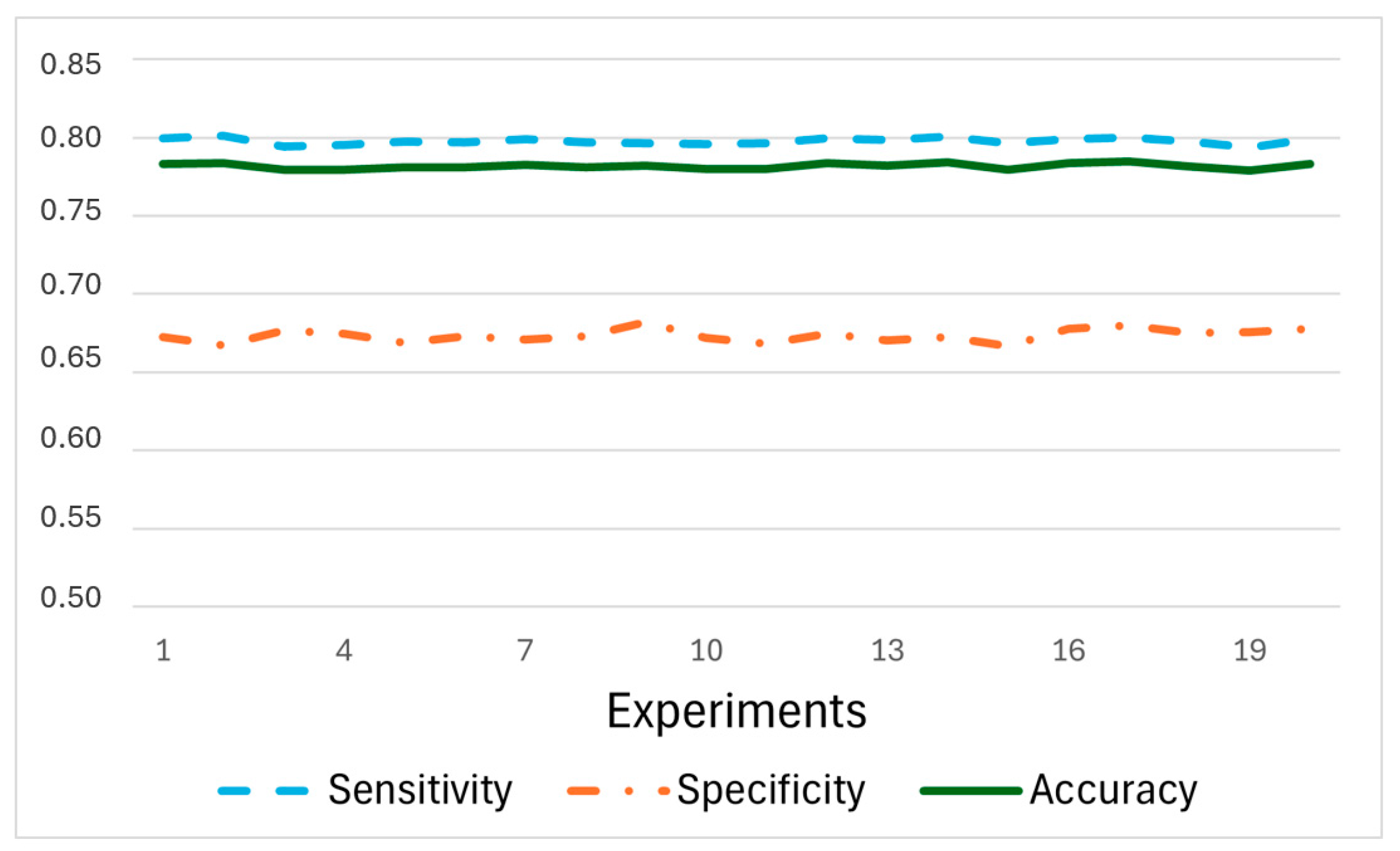
To ensure stable results, this study implemented 20 experiments using different separations of training and testing datasets. Figure 8 shows three common metrics (specificity, sensitivity, and accuracy) for evaluating the performance of the developed RF model under different training and testing. Through the twenty experiments, negligible fluctuations were observed in these metrics, underscoring the stability of the model. In comparison to specificity, sensitivity demonstrated relatively stable performance, fluctuating around 0.8. This fluctuation appeared due to the varied usage of training data and testing data. Specificity exhibited relatively lower values, hovering around 0.68. This suggests that incidents with unsuccessful responses might involve more complex situations and diverse geographic characteristics. Significantly fewer unsuccessful responses (30,169) than successful responses (205,242) also contributed to the model’s lack of accuracy in negative predictions, reflecting its lower specificity compared to sensitivity. To provide a more comprehensive evaluation of classification performance under class imbalance, additional metrics were calculated based on the confusion matrix of the testing dataset. The balanced accuracy, which accounts for performance across both majority and minority classes, was 0.734. Precision for the successful class reached 0.944, indicating that the majority of predicted successful dispatches were correctly identified. The F1-score, balancing precision and recall, was 0.857, reflecting strong overall classification performance. Furthermore, the G-Mean, which evaluates the balance between sensitivity and specificity, was 0.732, suggesting that the model maintains relatively stable performance across both classes despite the imbalanced distribution of outcomes.
Figure 8.
Model performance across 20 experiments with different random splits of the training and testing datasets. Sensitivity, specificity, and accuracy remain stable across experiments, indicating the robustness of the classification model to variations in data partitioning.
3.2. Spatial Autocorrelation in Residuals
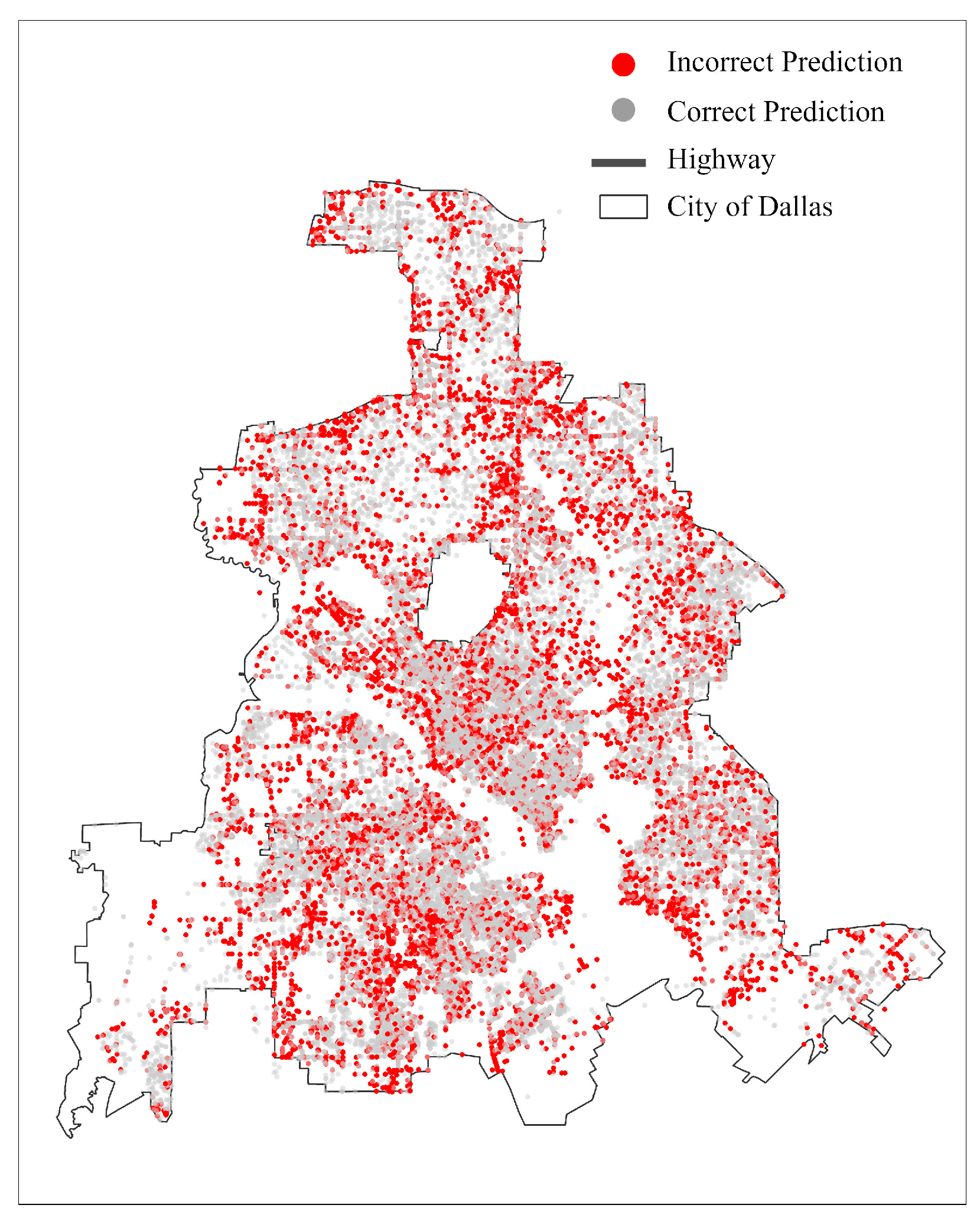
The spatial distribution of model performance was examined by mapping prediction outcomes across the city of Dallas, distinguishing between correct predictions (cases where the model correctly predicted emergency dispatch outcomes as successful or unsuccessful) and incorrect predictions (cases where the model misclassified the dispatch outcome) (Figure 9). Overall, among the 70,624 emergency incidents, the model correctly predicted 54,565 incidents (approximately 77.26%), while 15,699 incidents (approximately 22.74%) were misclassified. To further examine whether prediction errors exhibit spatial structure, we calculated Moran’s I on model residuals. Because the model outcome is binary (0 or 1), residuals were defined as the difference between the observed dispatch outcome and the predicted probability of a successful dispatch for each incident. For example, if a successful dispatch (observed value = 1) was predicted with a probability of 0.6, the residual is 0.4 (1 − 0.6). Conversely, if an unsuccessful dispatch (observed value = 0) was predicted with a probability of 0.6, the residual is −0.6 (0 − 0.6). This formulation produces continuous residual values that can be used to assess spatial autocorrelation.
Figure 9.
Spatial distribution of prediction outcomes from the random forest model for emergency dispatch across the city of Dallas. Red points represent incidents that were incorrectly classified by the model, while gray points indicate correctly classified cases.
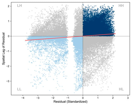
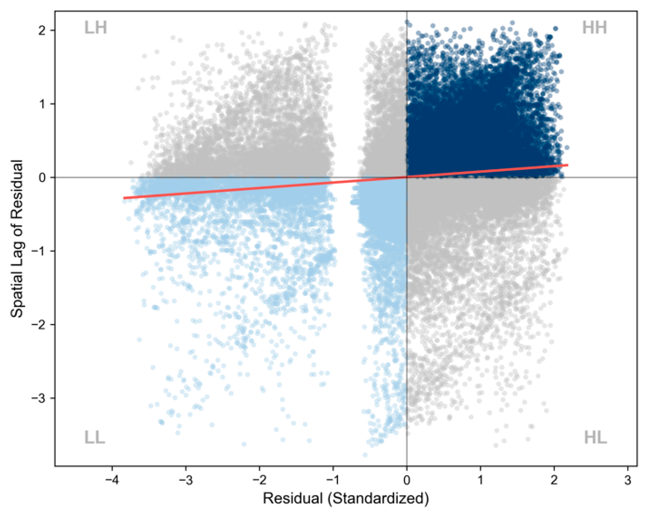
Global Moran’s I result indicates a small but statistically significant level of spatial autocorrelation in the residuals (Moran’s I = 0.0743, z = 26.24, p < 0.01) (Figure 10 and Table 3). While the model errors are not completely random across the space, the considerably low Moran’s I value indicates that the spatial clustering of prediction errors is weak as micro clusters and geographic separations results from non-populated areas and an enclosed area that is not part of the city (Figure 9). In other words, misclassifications do not exhibit strong spatial concentration across the study area.
Figure 10.
Moran’s I scatterplot of model residuals for emergency dispatch predictions. The horizontal axis represents standardized residual values, and the vertical axis shows the spatial lag of residuals based on neighboring incidents.
Table 3.
Global Moran’s I statistics for spatial autocorrelation in model residuals.
3.3. Importance of Geographical Variables to RF Model Prediction
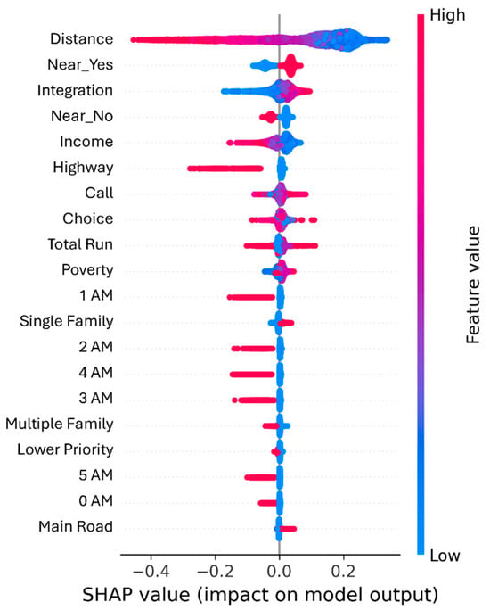
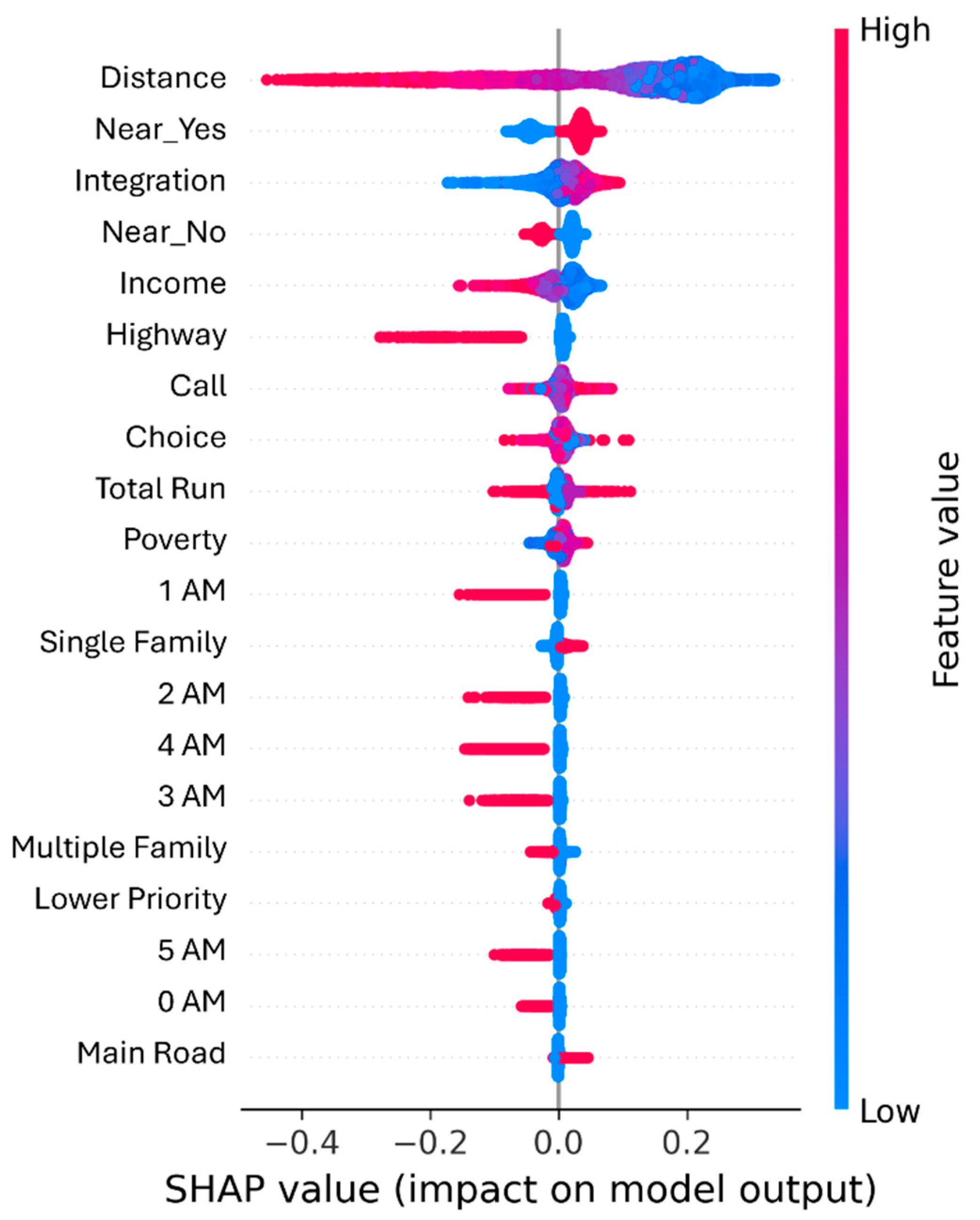
This study applied the Shapley additive explanations (SHAP) tool to enhance the transparency and interpretability of the random forest model, enabling an assessment of the contributions of each explanatory variable to model prediction. Figure 11 highlights the top twenty most important variables and presents an informative summary of their influence on the output of the prediction model. Each emergency incident in the testing dataset represents a point for each variable on the beeswarm plot. The color of each point (red shades vs. blue shades) reflects the raw values of the variables for each emergency incident. The variables on the left side were arranged in descending order based on their contribution to the model’s prediction. The points were distributed horizontally along the x-axis by their SHAP values, computed utilizing Equation (1). Positive SHAP values represent conditions that increase the likelihood of successful emergency dispatch, whereas negative SHAP values denote geographic characteristics that impede response.
Figure 11.
A SHAP summary plot of the explanatory variables in the random forest model. Variables are ranked by their overall importance based on the magnitude of SHAP values. Each point represents an observation, and the horizontal position indicates the contribution of a variable to the model’s output. Colors represent the relative magnitude of the feature value (blue = low, red = high).
3.3.1. Distance-Related Variables
Network distance has the strongest and most systematic influence on model output. Incidents that occurred farther from the Fire Rescue Department consistently produced large negative SHAP values, indicating that spatial separation remains the most significant barrier to timely arrival. Importantly, the distribution reveals a one-sided sensitivity: the model reacts strongly when the distance is long but exhibits little variation when the distance is short. In other words, proximity to an EMS location does not guarantee a better outcome, but being far away almost guarantees a worse one. Complementary to this effect, dispatches originating from the nearest station (Near_Yes) increased the likelihood of a successful response, whereas calls assigned to non-nearest stations (Near_No) were associated with a higher likelihood of unsuccessful arrival.
3.3.2. Spatial Accessibility
Spatial accessibility, represented by integration measures, also exhibited a clear directional pattern. Higher values of integration, which capture the degree to which locations are embedded within the broader street network, showed predominantly positive SHAP contributions. It implies that well-connected areas facilitate more efficient routing, enabling emergency vehicles to capitalize on multiple path options and fewer structural bottlenecks. Conversely, calls located in low-integration areas—often characterized by cul-de-sacs, fragmented residential blocks, or irregular street geometries—shifted the SHAP values toward the negative range, suggesting that network structure constrains vehicular mobility independent of distance alone. Choice reflects how frequently a street segment lies on the shortest paths between any origin–destination pairs of locations across the city. A higher choice value has conflicting effects on EMS responses: it suggests higher traffic volume, which can hinder EMS responses, yet it also suggests greater route options and accessibility, which facilitate EMS arrivals. The effects of high-choice street segments on EMS responses would likely be time dependent in relation to local traffic dynamics. As congestion on these segments varies throughout the day, their effectiveness in facilitating rapid response similarly fluctuates. These dynamics generate both positive and negative SHAP contributions, ultimately shaping the mixed distribution pattern observed in the model’s results.
3.3.3. Socioeconomic Status and Land Use
Socioeconomic and land use characteristics introduced additional spatial complexity to emergency response performance. Contrast to findings in the literature, the SHAP values in this study suggest that higher-income census tracts in Dallas had a greater likelihood of unsuccessful dispatch outcomes (i.e., negative SHAP values). A complementary measure (Poverty)—the proportion of households below 200% of the Federal Poverty Level—showed a similar pattern, with lower poverty areas shifting SHAP values toward less favorable predictions. Prior studies report mixed effects of SES on EMS performance. Hsia et al. (2018) [6] found that economically advantaged neighborhoods generally receive faster EMS responses at an aggregated level. In contrast, Seim et al. (2018) [8] observed that a 10-percentage-point increase in tract-level poverty corresponded to a 24 s decrease in median ambulance response time. The differences likely arise from the ways in which the income and poverty variables are evaluated. Mixed-effect modeling assumes linearity, homoscedasticity, and normal distributions of random effects. As random forest modeling accounts for nonlinear relationships and heterogeneity, the effect of each variable on model output is therefore nonlinear and heterogeneous. Moreover, SHAP contrasts model predictions from multiple simulations with versus without these variables and constraints that the sum of effects from all variables equals the model’s output for each incident. Therefore, the SHAP values of income and poverty are subject to the SHAP values of the other variables. Building upon this empirical observation, we offered a contextual interpretation grounded in existing urban studies literature. Beyond SES alone, urban development patterns—closely linked to higher socioeconomic status—add another layer of influence. Higher-income neighborhoods typically experience more frequent infrastructure investment, redevelopment, and roadway improvements [36]. These activities generate recurring construction events, which create temporary but significant mobility constraints for emergency vehicles through lane closures, detours, and pavement work. Trowbridge et al. (2009) [15] demonstrated that elements of urban sprawl, particularly roadway construction and development-related disruptions, are significantly associated with longer EMS response times.
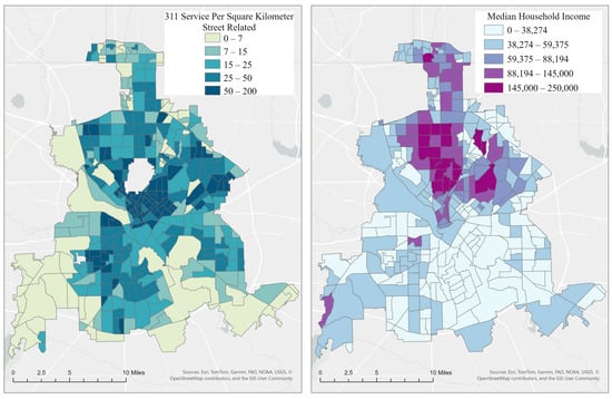
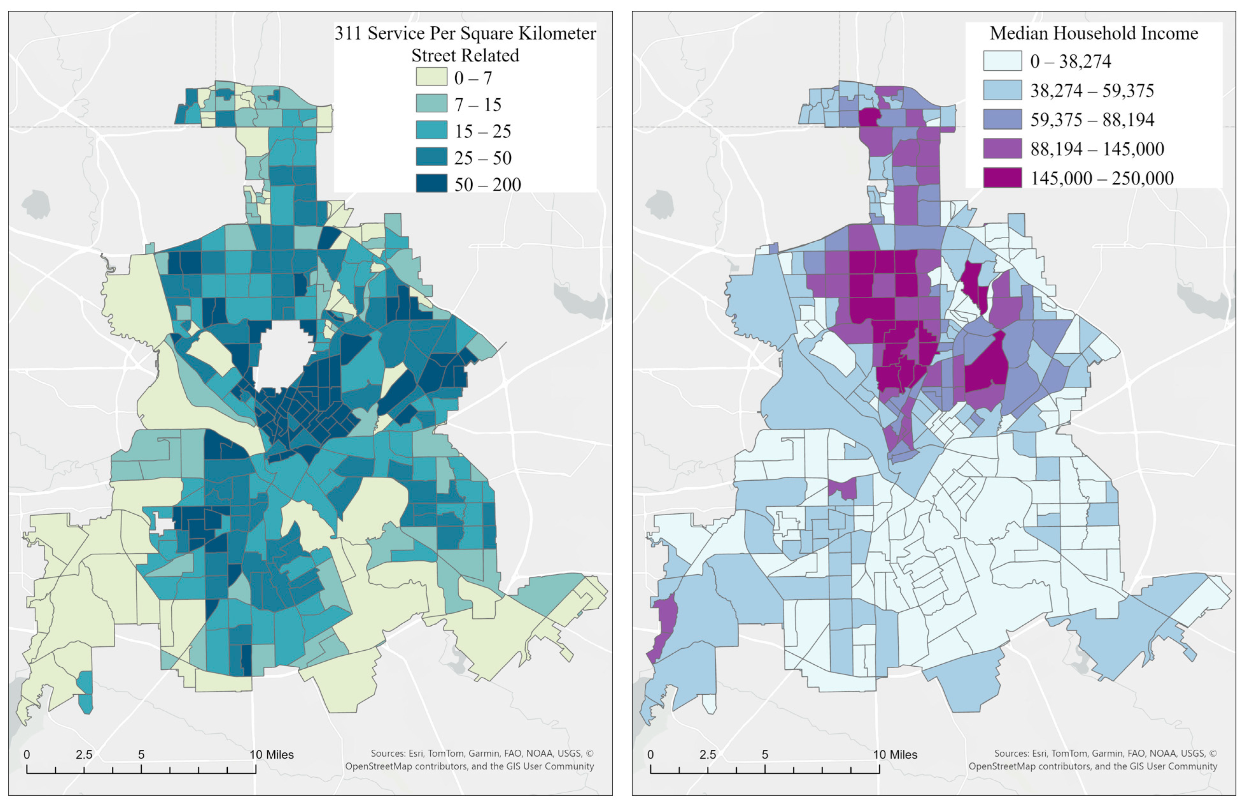
To examine this mechanism directly, we integrated street-related 311 service requests for 2016 in the City of Dallas, focusing on construction, street closures, and pavement-related disruptions (Appendix B. Table A1). As shown in Figure 12, tracts with higher median household incomes—particularly those in northern Dallas, where affluent communities cluster—reported substantially more street construction-related complaints (311). Elevated counts also appeared in portions of southwestern Dallas, indicating additional hotspots of roadway disturbance across the city. Both maps are projected using the NAD_1983_StatePlane_Texas_North_Central_FIPS_4202_Feet coordinate system, with north oriented upward.
Figure 12.
(Left) 311 street-related service requests per km2 across census tracts in Dallas, Texas, representing the spatial distribution of reported street maintenance issues; (Right) median household income across census tracts, illustrating the socioeconomic variation within the city of Dallas.
Together, these spatial patterns suggest that construction-driven street disruptions—common in higher-SES areas undergoing continuous urban development—may contribute to the higher likelihood of unsuccessful emergency dispatch observed in wealthier tracts. While higher-income neighborhoods may benefit from urban investments, the resulting construction activities can hinder emergency vehicle dispatch and counter the presumed benefits of socioeconomic advantage. This dynamic highlights the importance of considering SES not in isolation, but in conjunction with the evolving built environment that shapes emergency response accessibility.
Among land use variables, single-family and multi-family residential areas exerted the strongest influence on model predictions. This is expected given that residential land constitutes roughly 35% of Dallas’s urban fabric and typically accounts for a large share of emergency incidents (e.g., in this study, ). The structural characteristics of this land use type help explain their divergent effects: single-family parcels showed more successful dispatches likely due to clearly identifiable house numbers, whereas multi-family developments—often containing multiple units within a single structure—were associated with higher rates of unsuccessful arrival, likely due to the greater difficulty in pinpointing exact destinations.
3.3.4. Influence of Temporal Variables
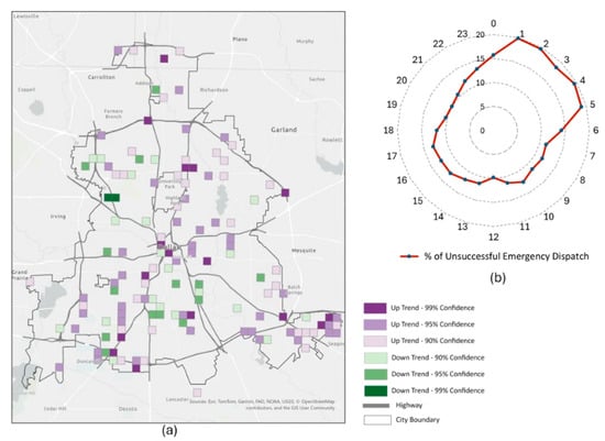
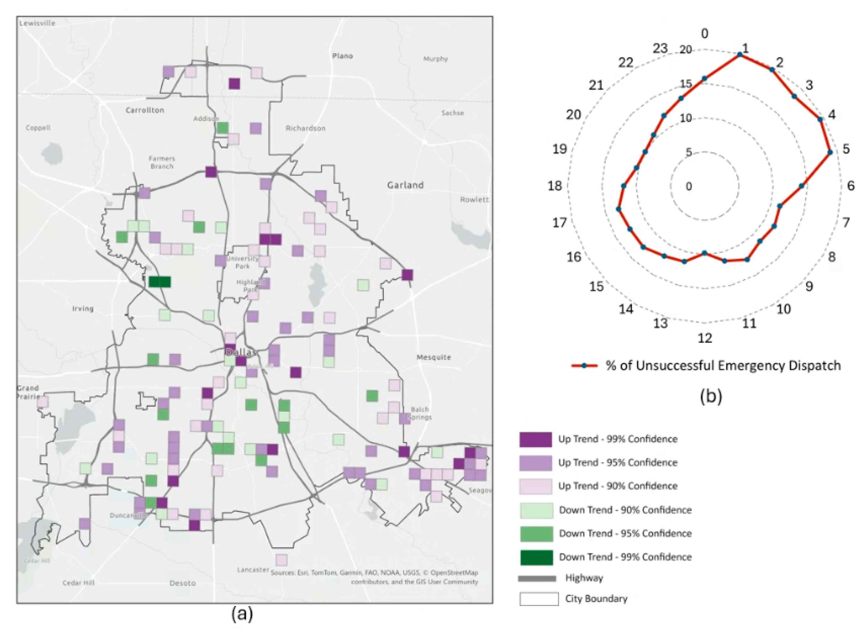
Among the temporal variables, the SHAP analysis showed that hour of day exerted a stronger influence on model predictions than day of week. In particular, the early-morning period between 1:00 AM and 5:00 AM increased the likelihood of unsuccessful emergency dispatches, as indicated by the concentration of red SHAP points extending toward the negative range. To further examine this pattern, we aggregated the proportion of unsuccessful dispatches across the 24 h cycle (Figure 13b). Between 1:00 AM and 5:00 AM, each hour shows approximately 20% of emergency dispatches being unsuccessful, nearly double the 10% observed during the subsequent morning and daytime hours. Furthermore, we aggregated unsuccessful dispatches using a 1000 m grid and 1 h interval framework to elucidate the spatial–temporal structure of the pattern. A Mann–Kendall trend test was subsequently applied to each grid cell to detect significant upward or downward trends across the 24 h cycle (Figure 13a). This analysis identified locations characterized by elevated early-morning failure rates followed by significant declines later in the day (green grid cells), as well as areas with comparatively lower early-morning failure rates that exhibit increasing trends over subsequent hours (purple grid cells). Collectively, these findings underscore the localized and time-sensitive variability in emergency response performance across the city.
Figure 13.
(a) Spatial–temporal trends in unsuccessful emergency dispatches across the study area, where each grid cell represents the direction and statistical significance of temporal trends detected using the Mann–Kendall test. (b) Hourly distribution of % unsuccessful emergency dispatches over 24 h, illustrating temporal variation in dispatch outcomes throughout the day.
Taken together, the SHAP outputs demonstrate that a complex interplay of spatial and operational factors shaped the ability of emergency services to reach incidents within critical time thresholds in 2016 Dallas EMS responses. Distance and network accessibility emerged as the dominant geographic determinants, while socioeconomic conditions, land use patterns, and temporal dynamics further modulated performance. These findings affirm that emergency response is not solely an operational problem but a deeply geographical one, embedded in the physical organization of urban space. Understanding these spatial effects provides a foundation for redesigning station allocations, improving dispatch protocols, and identifying structural inequities in emergency access across the urban landscape.
4. Conclusions
This study advances the understanding of emergency dispatch performance by examining geographic relationships at the individual incident level, rather than relying on aggregated counts of incidents or runs as in previous research. The study shows that where incidents occurred matters in getting timely EMS responses and reveals many nuances in the effects of geographic variables. In addition to geographic variables commonly used in the literature, we introduced integration and choice as street-level spatial accessibility measures to evaluate how the configuration of the urban street network influences emergency dispatch outcomes. To the best of our knowledge, no prior studies have systematically assessed the impact of spatial accessibility on emergency response at this level of spatial resolution.
We employed random forest models to evaluate the influence of geographical features on dispatch performance, framed as a binary outcome. The model achieved a sensitivity of 78.58% for predicting successful emergency dispatches and 68.26% for predicting unsuccessful dispatches, using 14 variables that encompassed both street-level road characteristics and area-level socioeconomic features. The model’s performance is moderate compared to other random forest applications because this study only considered geographic variables and related temporal variables in EMS responses. Other operational and policy variables, such as EMS equipment inventory, human resources, and dispatch strategies, are not considered. As such, this study shows where matters with consequential geographic effects on timely EMS responses. According to the SHAP analysis, integration emerged as the third most important predictor in the model. The distribution of SHAP values for integration on the beeswarm plot further illustrates its role. Notably, observations with higher integration values clustered near the center of the SHAP axis, whereas those with lower integration values extended further toward the right. This asymmetric spread indicates that low integration—reflecting poorer spatial accessibility—had a stronger influence on predicting unsuccessful responses (=0) than high integration did on predicting successful responses (=1). In other words, spatial accessibility appears to play a more substantial role in shaping incidents that result in unsuccessful emergency responses.
Regarding socioeconomic indicators, they alone are insufficient to explain disparities in emergency response performance, and past research has largely overlooked the geographic dynamics that accompany socioeconomic advantage. Higher-income areas are not static beneficiaries of better services but are often active sites of redevelopment, infrastructure upgrades, and recurrent road maintenance—processes that can temporarily degrade emergency accessibility. This finding calls for a shift in future EMS research toward models that explicitly integrate dynamic, fine-scale urban processes such as construction cycles, road obstructions, redevelopment intensity, and real-time mobility constraints. For policymakers and city governments, this implies that improving emergency response requires not only considering socioeconomic issues but also coordinating public works, transportation departments, and emergency services to anticipate and mitigate the impact of construction and infrastructure projects. Integrating EMS routing with live street-level data, scheduling major works with emergency accessibility in mind, and adopting proactive cross-departmental planning will be critical steps toward more resilient and equitable urban emergency systems. Additionally, socioeconomic variables measured at finer spatial scales, such as census block groups, can better capture socioeconomic heterogeneity.
The temporal distribution of unsuccessful emergency responses shows a distinct increase during the early-morning hours compared with other time periods, further supporting our conclusion regarding the importance of temporal effects. In contrast, the spatial–temporal analysis does not reveal a clear geographic pattern, as no prominent clusters appear across the grid cells. Prior research offers a possible explanation for this pattern, although fatigue is not directly measured in our dataset. Takeyama et al. (2005) [37], in a 17-day field study of firefighters, reported that the time window between 1 a.m. and 5 a.m. is associated with markedly higher levels of subjective fatigue and physiological complaints than other periods of the day. Similarly, interview data from 15 participants collected through the National Fire Academy indicate that disrupted sleep patterns and intensive workloads during high-call periods (9 PM–11 PM) substantially elevate fatigue levels, helping to explain the early-morning peak in exhaustion. Moreover, research [38] on the effects of fatigue among emergency responders has shown that fatigue impacts on cognitive function and alertness. Taken together, the consistency between our results and existing research suggests that fatigue and psychological strain play a critical role in dispatch performance. Future research should incorporate psychological and physiological assessments to more fully understand how these factors influence the likelihood and mechanisms of dispatch failure.
This study aimed to develop an explanatory modeling framework to advance our understanding how geographical variables influence emergency dispatch outcomes, rather than serving as a benchmarking exercise focused on predictive algorithm comparison. Accordingly, the random forest model was selected for its ability to capture nonlinear relationships and complex interactions among spatial and operational variables, and SHAP was employed to enhance interpretability. The emphasis of this study therefore lies in identifying and interpreting influential geographical factors rather than optimizing predictive performance across competing models. Future research can extend this study by incorporating baseline models, such as logistic regression or other parametric approaches, to systematically compare predictive performance and further evaluate the robustness of the identified spatial relationships.
Emergency incident types in this study were reclassified into three categories following the operational definitions established by the Fire and EMS Department in the city of Dallas. Future research could further investigate this dimension using more fine-grained, event-level classifications. The eight-minute threshold provides a practical benchmark widely used in emergency response evaluation. However, converting response time into a binary classification around a fixed cutoff may obscure variation among incidents near the threshold. Future research could examine the sensitivity of model outcomes to alternative thresholds or model response time as a continuous variable to capture more nuanced variation in emergency response performance.
5. Limitations
There are several limitations in this study. Firstly, besides focusing on geographic factors beyond EMS operations, policy, and human resources, this study was limited by its inability to elucidate the influence of spatial scale on emergency response analysis. Using varying spatial analysis units may lead to different outputs, which is known as the scale effect. As a significant concept in geography, the scale effect manifests in a wide range of geographic phenomena [39]. As a suggestion for future research, conducting comparative studies could offer valuable insights into the impact of spatial scale on machine learning predictive models. By examining various spatial scales, such as street-level, census tract, block group, and defined grid scales, researchers can better understand how the choice of spatial scale affects the performance and outcomes of predictive modeling in the context of emergency response. Secondly, this study employed stratified sampling to partition the training and testing datasets. Future research could incorporate spatial cross-validation strategies to further evaluate model robustness while accounting for potential spatial autocorrelation in emergency incident data. Thirdly, although temporal variables such as hour of day and day of week were included to capture systematic variations in urban traffic conditions, this study does not incorporate direct measures of traffic congestion or travel time variability. Traffic conditions are widely recognized as important determinants of emergency response performance, as congestion can significantly delay emergency vehicle movement. Future research could integrate real-time or historical traffic datasets to further examine how congestion and travel time variability influence emergency response outcomes.
Author Contributions
Yanan Wu: methodology development; software; investigation; validation of results; formal analysis; data curation; writing—original draft preparation. Yalin Yang: methodology development; data curation; software; validation of results. May Yuan: conceptualization, validation of results; formal analysis; investigation; writing—review and editing; supervision; project management. All authors have read and agreed to the published version of the manuscript.
Funding
This research received no external funding.
Data Availability Statement
The data that support the findings of this study were provided by the Dallas Fire Rescue Department and were used under formal approval for the current study. Due to data-use restrictions, the datasets are not publicly available.
Acknowledgments
We gratefully acknowledge the Dallas Fire Rescue Department for providing the data used in this study. The research was funded by the U.S. National Institute of Standards and Technology through Grant No. 60NANB17D180. The content is solely the responsibility of the authors and does not necessarily represent the official views of the Dallas Fire Rescue Department or the National Institute of Standards and Technology.
Conflicts of Interest
The authors declare no conflicts of interest.
Abbreviations
The following abbreviations are used in this manuscript:
| EMS | Emergency medical service |
| UAVs | Uncrewed aerial vehicles |
| NFPA | National fire protection association |
| SES | Socioeconomic status |
| ML | Machine learning |
| GPS | Global positioning system |
| CAD | Computer-Aided dispatch |
| CDR | Call detailed records |
| ACS | American community survey |
| TxDOT | Texas department of transportation |
| NCTCOG | North central Texas council of governments |
| RF | Random forest |
| BO | Bayesian optimization |
| SHAP | Shapley additive explanations |
Appendix A
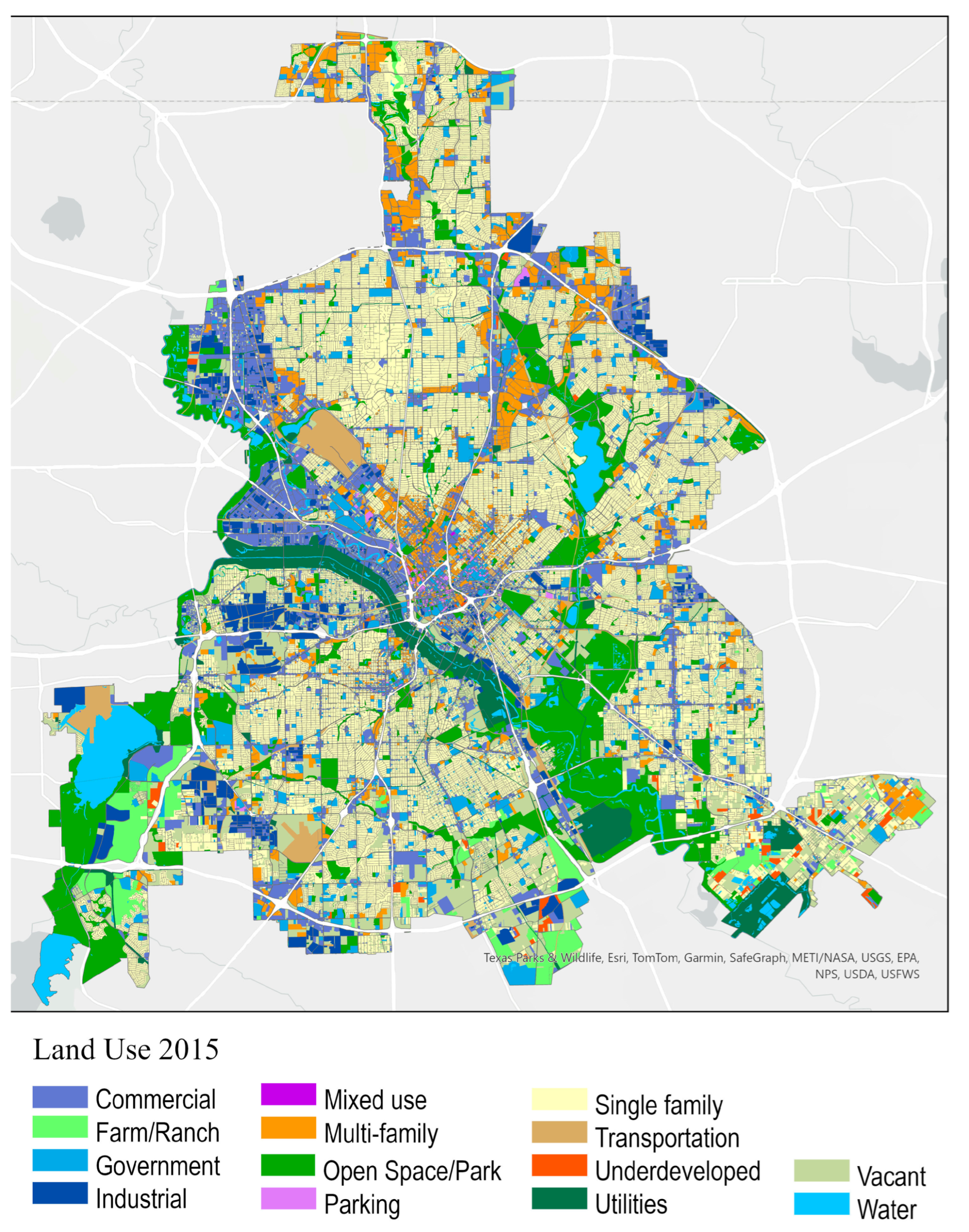
Land Use Map for 2015 (City of Dallas) from Regional Data Center NCTCOG, Map Is Projected Using the NAD_1983_StatePlane_Texas_North_Central_FIPS_4202_Feet Coordinate System, with North Oriented Upward
Figure A1.
Land use map for 2015 (city of Dallas) from Regional Data Center NCTCOG.
Appendix B
Table A1.
Street-related 311 Service Request Type in 2016.
References
- Vanga, S.R.; Ligrani, P.M.; Doustmohammadi, M.; Anderson, M. EMS Response Time for Patients Critically-Injured from Automobile Accidents Using Regression Analysis. Curr. Urban Stud. 2021, 09, 581–596. [Google Scholar] [CrossRef]
- Stevens, J.M.; Webster, T.C.; Stipak, B. Response Time: Role in Assessing Police Performance. Public Product. Rev. 1980, 4, 210–230. [Google Scholar] [CrossRef] [Scilit]
- Gao, X.; Kong, N.; Griffin, P. Shortening Emergency Medical Response Time with Joint Operations of Uncrewed Aerial Vehicles with Ambulances. Manuf. Serv. Oper. Manag. 2024, 26, 447–464. [Google Scholar] [CrossRef] [Scilit]
- Yu, W.; Bai, W.; Luan, W.; Qi, L. State-of-the-Art Review on Traffic Control Strategies for Emergency Vehicles. IEEE Access 2022, 10, 109729–109742. [Google Scholar] [CrossRef] [Scilit]
- Bandyopadhyay, M.; Singh, V. Development of Agent Based Model for Predicting Emergency Response Time. Perspect. Sci. 2016, 8, 138–141. [Google Scholar] [CrossRef] [Scilit]
- Hsia, R.Y.; Huang, D.; Mann, N.C.; Colwell, C.; Mercer, M.P.; Dai, M.; Niedzwiecki, M.J. A US National Study of the Association Between Income and Ambulance Response Time in Cardiac Arrest. JAMA Netw. Open 2018, 1, e185202. [Google Scholar] [CrossRef] [Scilit]
- Meurer, W.J.; Levine, D.A.; Kerber, K.A.; Zahuranec, D.B.; Burke, J.; Baek, J.; Sanchez, B.; Smith, M.A.; Morgenstern, L.B.; Lisabeth, L. Neighborhood Influences on Emergency Medical Services Use for Acute Stroke: A Population-Based Cross-Sectional Study. Ann. Emerg. Med. 2016, 67, 341–348. [Google Scholar] [CrossRef] [Scilit] [PubMed]
- Seim, J.; Glenn, M.J.; English, J.; Sporer, K. Neighborhood Poverty and 9-1-1 Ambulance Response Time. Prehospital Emerg. Care 2018, 22, 436–444. [Google Scholar] [CrossRef] [Scilit] [PubMed]
- Wakefield, J.; Lyons, H. Spatial Aggregation and the Ecological Fallacy. Handb. Spat. Stat. 2010, 20103158, 541–558. [Google Scholar]
- Mclay, L.A.; Mayorga, M.E. Evaluating Emergency Medical Service Performance Measures. Health Care Manag. Sci. 2010, 13, 124–136. [Google Scholar] [CrossRef] [Scilit]
- Zayed, S.; Al-Shaqsi, K. Response Time as a Sole Performance Indicator in EMS: Pitfalls and Solutions. Open Access Emerg. Med. 2010, 2, 1–6. [Google Scholar]
- Bailey, E.D.; Sweeney, T. Considerations in Establishing Emergency Medical Services Response Time Goals. Prehospital Emerg. Care 2003, 7, 397–399. [Google Scholar] [CrossRef] [Scilit] [PubMed]
- Blanchard, I.E.; Doig, C.J.; Hagel, B.E.; Anton, A.R.; Zygun, D.A.; Kortbeek, J.B.; Gregory Powell, D.; Williamson, T.S.; Fick, G.H.; Innes, G.D. Emergency Medical Services Response Time and Mortality in an Urban Setting. Prehospital Emerg. Care 2012, 16, 142–151. [Google Scholar] [CrossRef] [Scilit] [PubMed]
- Pons, P.T.; Markovchick, V.J. Eight Minutes or Less: Does the Ambulance Response Time Guideline Impact Trauma Patient Outcome? J. Emerg. Med. 2002, 23, 43–48. [Google Scholar] [CrossRef] [Scilit]
- Trowbridge, M.J.; Gurka, M.J.; O’Connor, R.E. Urban Sprawl and Delayed Ambulance Arrival in the U.S. Am. J. Prev. Med. 2009, 37, 428–432. [Google Scholar] [CrossRef] [Scilit] [PubMed]
- Concannon, T.W.; Griffith, J.L.; Kent, D.M.; Normand, S.L.; Newhouse, J.P.; Atkins, J.; Beshansky, J.R.; Selker, H.P. Elapsed Time in Emergency Medical Services for Patients with Cardiac Complaints Are Some Patients at Greater Risk for Delay? Circ. Cardiovasc. Qual. Outcomes 2009, 2, 9–15. [Google Scholar] [CrossRef] [Scilit]
- Griffin, R.; McGwin, G. Emergency Medical Service Providers’ Experiences with Traffic Congestion. J. Emerg. Med. 2013, 44, 398–405. [Google Scholar] [CrossRef] [Scilit]
- Lee, J.; Abdel-Aty, M.; Cai, Q.; Wang, L. Analysis of Fatal Traffic Crash-Reporting and Reporting-Arrival Time Intervals of Emergency Medical Services. Artic. Transp. Res. Rec. 2018, 2672, 61–71. [Google Scholar] [CrossRef] [Scilit]
- Fu, X.; Nie, Q.; Li, X.; Liu, J.; Nambisan, S.; Jones, S. The Role of the Built Environment in Emergency Medical Services Delays in Responding to Traffic Crashes. J. Transp. Eng. Part A Syst. 2022, 148, 04022085. [Google Scholar] [CrossRef] [Scilit]
- Hillier, B.; Iida, S. Network and Psychological Effects in Urban Movement. In Spatial Information Theory, Proceedings of the International Conference; Springer: Berlin/Heidelberg, Germany, 2005; pp. 475–490. [Google Scholar]
- Ewing, R.; Tian, G.; Lyons, T. Does Compact Development Increase or Reduce Traffic Congestion? Cities 2018, 72, 94–101. [Google Scholar] [CrossRef] [Scilit]
- Peng, C.; Jin, X.; Wong, K.C.; Shi, M.; Liò, P. Collective Human Mobility Pattern from Taxi Trips in Urban Area. PLoS ONE 2012, 7, e0034487. [Google Scholar] [CrossRef] [Scilit]
- Hillier, B. Space Is the Machine: A Configurational Theory of Architecture; Space Syntax: London, UK, 2007. [Google Scholar]
- Johnsson, C.; Camporeale, R. Exploring Space Syntax Integration at Public Transport Hubs and Public Squares Using Drone Footage. Appl. Sci. 2022, 12, 6515. [Google Scholar] [CrossRef] [Scilit]
- Hillier, B.; Burdett, R.; Peponis, J.; Penn, A. Creating Life: Or, Does Architecture Determine Anything? Archit. Comport./Archit. Behav. 1986, 3, 233–250. [Google Scholar]
- Othman, F.; Yusoff, Z.M.; Salleh, S.A. Assessing the Visualization of Space and Traffic Volume Using GIS-Based Processing and Visibility Parameters of Space Syntax. Geo-Spat. Inf. Sci. 2020, 23, 209–221. [Google Scholar] [CrossRef] [Scilit]
- Smith, J.P. The Impact of Socioeconomic Status on Health over the Life-Course. J. Hum. Resour. 2007, 42, 739–764. [Google Scholar] [CrossRef] [Scilit]
- Moore, L.V.; Diez Roux, A.V.; Evenson, K.R.; McGinn, A.P.; Brines, S.J. Availability of Recreational Resources in Minority and Low Socioeconomic Status Areas. Am. J. Prev. Med. 2008, 34, 16–22. [Google Scholar] [CrossRef] [Scilit]
- Kleindorfer, D.O.; Lindsell, C.J.; Broderick, J.P.; Flaherty, M.L.; Woo, D.; Ewing, I.; Schmit, P.; Moomaw, C.; Alwell, K.; Pancioli, A.; et al. Community Socioeconomic Status and Prehospital Times in Acute Stroke and Transient Ischemic Attack: Do Poorer Patients Have Longer Delays from 911 Call to the Emergency Department? Stroke 2006, 37, 1508–1513. [Google Scholar] [CrossRef] [Scilit]
- Fleischman, R.J.; Lundquist, M.; Jui, J.; Newgard, C.D.; Warden, C. Predicting Ambulance Time of Arrival to the Emergency Department Using Global Positioning System and Google Maps. Prehospital Emerg. Care 2013, 17, 458–465. [Google Scholar] [CrossRef] [Scilit] [PubMed]
- Ataman, M.G.; Sarıyer, G. Predicting Waiting and Treatment Times in Emergency Departments Using Ordinal Logistic Regression Models. Am. J. Emerg. Med. 2021, 46, 45–50. [Google Scholar] [CrossRef] [Scilit]
- Breiman, L. Random Forests. Mach. Learn. 2001, 45, 5–32. [Google Scholar] [CrossRef] [Scilit]
- Boeing, G. Street Network Models and Measures for Every U.S. City, County, Urbanized Area, Census Tract, and Zillow-Defined Neighborhood. Urban Sci. 2019, 3, 28. [Google Scholar] [CrossRef] [Scilit]
- Wu, Y.; Yang, Y.; Yuan, M. Location Analytics of Routine Occurrences (LARO) to Identify Locations with Regularly Occurring Events with a Case Study on Traffic Accidents. Information 2024, 15, 107. [Google Scholar] [CrossRef] [Scilit]
- Lundberg, S.; Lee, S.-I. A Unified Approach to Interpreting Model Predictions. Adv. Neural Inf. Process. Syst. 2017, 30, 4768–4777. [Google Scholar] [CrossRef] [Scilit]
- Ryan, A.; Christofa, E.; Barchers, C.; Knodler, M. The Relationship between Municipal Highway Expenditures and Socio-Demographic Status: Are Safety Investments Equitably Distributed? Transp. Res. Interdiscip. Perspect. 2021, 9, 100321. [Google Scholar] [CrossRef] [Scilit]
- Takeyama, H.; Itani, T.; Tachi, N.; Sakamura, O.; Murata, K.; Inoue, T.; Takanishi, T.; Suzumura, H.; Niwa, S. Effects of Shift Schedules on Fatigue and Physiological Functions among Firefighters during Night Duty. Ergonomics 2005, 48, 1–11. [Google Scholar] [CrossRef] [Scilit]
- Marvin, G.; Schram, B.; Orr, R.; Canetti, E.F.D. Occupation-Induced Fatigue and Impacts on Emergency First Responders: A Systematic Review. Int. J. Environ. Res. Public Health 2023, 20, 7055. [Google Scholar] [CrossRef] [Scilit]
- Atkinson, P.M.; Tate, N.J. Spatial Scale Problems and Geostatistical Solutions: A Review. Prof. Geogr. 2000, 52, 607–623. [Google Scholar] [CrossRef] [Scilit]

Disclaimer/Publisher’s Note: The statements, opinions and data contained in all publications are solely those of the individual author(s) and contributor(s) and not of MDPI and/or the editor(s). MDPI and/or the editor(s) disclaim responsibility for any injury to people or property resulting from any ideas, methods, instructions or products referred to in the content. |
© 2026 by the authors. Published by MDPI on behalf of the International Society for Photogrammetry and Remote Sensing. Licensee MDPI, Basel, Switzerland. This article is an open access article distributed under the terms and conditions of the Creative Commons Attribution (CC BY) license.