Article

Mapping Mental Wellbeing and Air Pollution: A Geospatial Data Approach

by
Morgan Ecclestone
and
Thomas Johnson
*
Department of Computer Science, Nottingham Trent University, Clifton Campus, Clifton Lane, Nottingham NG11 8NS, UK
*
Author to whom correspondence should be addressed.
ISPRS Int. J. Geo-Inf. 2026, 15(4), 142; https://doi.org/10.3390/ijgi15040142
Submission received: 4 November 2025 / Revised: 3 March 2026 / Accepted: 20 March 2026 / Published: 25 March 2026

Abstract

Urban air pollution is increasingly recognised as a determinant of mental wellbeing, yet most existing studies rely on static exposure estimates and lack spatial granularity. This limits understanding of how pollutant-specific patterns influence psychological states in real-world settings. To address this gap, we integrate real-time environmental and physiological data from 40 participants using the DigitalExposome dataset, applying multivariate and spatial analysis techniques. Our findings confirm that Particulate Matter (PM2.5) exerts the strongest negative association with mental wellbeing while extending prior work by establishing a preliminary ranking of other pollutants Particulate Matter (PM10), Particulate Matter (PM1), Carbon Monoxide (CO), Nitrogen Dioxide (NO2), Ammonia (NH3). We applied statistical and spatial analysis methods, including heatmaps and Voronoi diagrams, to explore links between pollutants and wellbeing and compare the relative influence of air pollution and noise. This enabled identification of pollutant-specific hotspots and multi-level wellbeing patterns across individual, accumulated, and collective scales. These results demonstrate the value of spatial analysis for environmental health research and support targeted urban interventions, such as green space placement and traffic re-routing, to mitigate mental wellbeing risks.

1. Introduction and Background

Air pollution is an increasingly pressing concern in the UK and globally, with well established impacts on physical health; including respiratory, cardiovascular, and neurological conditions—and emerging links to mental wellbeing [1,2]. According to the World Health Organisation (WHO), 99% of the global population lives in areas where air quality guidelines are not met, contributing to an estimated 4.2 million premature deaths annually [3], including over 48,000 per year in the UK [4]. Although the physiological effects of pollution are well documented, research into its psychological impacts remains comparatively limited, partly due to the complexity of quantifying mental wellbeing and the paucity of high resolution, individual-level data. Traditional studies often rely on coarse regional datasets and infrequent sampling, which obscure the dynamic and spatially heterogeneous nature of urban exposures and their influence on wellbeing [5,6].
A wide range of pollutants have been linked to poor health outcomes with Particulate Matter (PM), especially PM2.5 can penetrate deep into the lungs and bloodstream, and has been associated with oxidative stress, increased mortality, and multi-organ impacts including neurological effects [7,8,9]. Nitrogen oxides (NOx) and sulphur oxides (SOx) arising from traffic and industrial sources contribute to respiratory irritation and secondary pollutant formation, with NO2 capable of reaching the alveoli and entering the bloodstream [10,11,12]. Carbon Monoxide (CO) binds to haemoglobin, causing tissue hypoxia and long-term neurological sequelae in survivors [13]. Ground level ozone (O3), formed photochemically from NO2 and volatile organic compounds, is linked to respiratory distress and rising ozone related mortality [12,14]. Beyond chemical exposures, noise pollution is a significant environmental stressor; chronic exposure especially from transport has been associated with sleep disturbance, emotional distress, depression, anxiety, and cardiovascular disease, with adverse effects observed at levels as low as 45 dB [3,15].
The UK’s continued migration towards cities now comprising approximately 85% of the population places more individuals in proximity to traffic corridors and industrial zones, where PM2.5 and NO2 concentrations are elevated [16,17]. Socio-spatial inequalities further compound risk: higher pollution levels are often observed along major roadways (e.g., motorways) and in economically deprived areas, correlating with increased disease burden related to NO2 and PM2.5 exposure [18,19]. Public awareness and regulatory responses such as tighter controls on diesel emissions given their comparatively high NOx output have driven measurable reductions; for instance, UK mortality attributable to PM2.5 and NO2 decreased by 56% and 44%, respectively, between 1970 and 2010 [20,21]. Nonetheless, the persistence of elevated exposures in dense urban settings keeps population risk high.
To better integrate the multiple environmental influences on health, the “Exposome” framework emphasises the totality of exposures across the life course [22]. It complements the genome by centring environmental determinants and is commonly articulated across internal (e.g., metabolism, genetics, stress), specific external (e.g., lifestyle, individual pollution exposures), and general external domains (e.g., ambient air quality, climate, access to green space) [23,24]. While physiological impacts of pollution within the Exposome are extensively studied, corresponding research into mental wellbeing remains less comprehensive, despite evidence of higher mental health disorder prevalence in urban versus rural contexts [25,26,27].
Compared to more defined organ systems, the brain’s complexity and interconnection with other systems make isolating single-factor effects difficult [28]. Quantifying mental wellbeing introduces variability across instruments and designs, leading to inconsistency in exposure–outcome methodologies [29]. While cellular and animal studies can demonstrate pollutant-specific mechanisms (e.g., O3-induced oxidative stress via oxeiptotic pathways) [30], translating these findings to real-world mental wellbeing requires multimodal, temporally resolved, ecologically valid human data [31,32]. Recent computational work (e.g., text derived wellbeing models) has found that Bag-of-Words and TF–IDF approaches can achieve strong performance, but these are often decoupled from continuous environmental measurements [33].
Advances in wearable sensing, edge computing, and ecological momentary assessment (EMA) now enable real-time study of person environment interactions [34,35]. On-body biosensors can collect continuous or high-frequency data on physiological arousal and environmental exposures, while edge devices reduce latency and enable privacy preserving local processing [36,37,38]. EMA via mobile applications prompts participants to self-report mood or wellbeing in situ, often using emoji or simple scales to reduce respondent burden and improve cross-user consistency [39,40]. These tools have been used to classify stress during examination periods, assess commuter mood under PM2.5 and NO2 exposure, and detect individuals at risk of mental health difficulties [41,42]. Complementary visualisation platforms—such as global Air Quality Index (AQI) heatmaps assist communication and exploratory analysis of spatiotemporal trends [43,44].
This study builds on these developments by utilising the DigitalExposome dataset [45], which comprises multimodal data from 40 participants collected in diverse urban environments. The dataset enables fine-grained spatial–temporal analysis of pollutant exposure and its relationship to momentary wellbeing, offering an opportunity to examine how specific pollutants; such as particulate matter and nitrogen dioxide correlate with physiological stress markers and subjective wellbeing states.
The major contributions of this work are:
  • Enhanced Real-World Data Integration: Building on our previous work, this study consolidates and analyses real-time environmental and physiological data from 40 participants using the DigitalExposome framework. It confirms and extends earlier findings by demonstrating that Particulate Matter (especially Particulate Matter2.5) and certain gases (Nitrogen Dioxide2) are negatively correlated with Inter-Beat Interval (IBI) and Electrodermal Activity (EDA), with improved spatial resolution and participant diversity.
  • Advanced Multivariate and Spatial Analysis Techniques: This study applies multivariate statistical methods including Principal Component Analysis (PCA), regression modelling, and novel spatial visualisations such as heatmaps and Voronoi Display. These techniques enable deeper exploration of pollutant–wellbeing relationships and support the identification of pollution hotspots with potential causal implications.
  • Multi-Level Spatial Wellbeing Representation: Wellbeing is visualised across three spatial-temporal levels: (i) Collective through aggregating wellbeing data from multiple participants across diverse urban contexts, (ii) Accumulated by mapping a participant’s wellbeing across multiple environments, and (iii) Individual through tracking a single participant’s wellbeing over time in a fixed environment.
The remainder of this paper is organised as follows. Section 2 introduces the core concept of this study and describes the DigitalExposome dataset, including its multimodal structure, data collection and study methodology. Section 3 presents the results, detailing the use of Principal Component Analysis (PCA) to assess variable importance and spatial techniques such as heatmaps and Voronoi Display, to explore individual-level impacts. Section 4 discusses the findings in the context of existing research, highlighting the implications and significance of the results. Finally, Section 5 concludes this paper and outlines directions for future research.

2. Data and Methods

2.1. DigitalExposome Data

The DigitalExposome dataset was developed as part of a research initiative to quantify the impact of urban environmental exposures on human wellbeing using multimodal sensor fusion techniques [45]. It integrates real-time environmental air quality data (including PM1, PM2.5, PM10, NO2, CO, NH3, and noise), physiological responses (such as heart rate variability and Electrodermal Activity), and self-reported wellbeing metrics collected via ecological momentary assessment (EMA). As detailed in the original published manuscript [45], data was gathered from 40 healthy adult participants (aged between 18–50) navigated a predefined urban route, enabling spatially and temporally aligned analysis of environmental stressors and physiological effects (Figure 1). The dataset’s high-resolution, real-world nature makes it particularly valuable for modelling short-term person–environment interactions and supports advanced analytical techniques such as multivariate analysis, spatial mapping, and machine learning.
A total of 42,437 samples were recorded using three synchronised data streams as discussed in [45], consisting of a low-cost Enviro-IoT, E4 Empatica and an Android Smartphone to collect self-report wellbeing labels as stated in the following:
  • Environmental Data: Measurements include Particulate Matter (PM1, PM2.5, PM10), Carbon Monoxide (CO), Ammonia (NH3), Nitrogen Dioxide (NO2), and ambient noise levels. These were sampled at 0.2 Hz using portable air quality sensors. The data was time-stamped at the point of collection.
  • Physiological Data: Captured via the E4 Empatica wearable device, this includes Electrodermal Activity (EDA) at 4 Hz, Heart Rate (HR) at 1 Hz, Blood Volume Pulse (BVP) at 64 Hz, and Inter-Beat Interval (IBI) as inter-beat intervals. All physiological signals were downsampled to 1 Hz to ensure temporal alignment across modalities. The data was time-stamped at the point of collection.
  • Perceived Wellbeing Data: Participant self-report of wellbeing in addition to a time stamp was obtained in the DigitalExposome study using a 5-point SAM affect scale consisting of five validated emojis ranging from 1 (very negative) to 5 (very positive). This approach is widely used in ecological momentary assessment (EMA) research, with substantial evidence demonstrating that short in-the-moment self-reports are reliable and sensitive to environmental fluctuations and well validated against both physiological and behavioural markers of affective state [46,47,48]. Self-report affect is considered an appropriate primary marker in EMA because it captures wellbeing in real time and reduces recall bias, which is a major limitation of retrospective questionnaires [49]. However, as with all self-report measures, these ratings may still be subject to momentary mood or individual interpretation of the scale.
The dataset was geo-tagged and time-stamped at the point of collection, enabling spatial–temporal analysis of environmental stressors and their physiological impacts. As the environmental and physiological data collected had varying sample rates, the following analysis was conducted using linear interpolation, as described in the original paper [46]. Physiological data (e.g., EDA, BVP, HRV and body temperature) were downsampled to a rate of 1Hz to match the sample rate of collected HR by the device. The environmental data was upsampled to match the sampled rate of the physiological data at 1Hz. Finally, the labelled data from the mobile smartphone was extracted and upsampled to the same rate as the environmental and physiological data to 1Hz to remain consistent with the other data. The fusion of these data streams supports robust modelling of the exposome and its influence on momentary wellbeing.

2.2. Presentation and Statistical Description of Raw Data

To explore the correlations between environmental, physiological and self-reported wellbeing, several statistical data description approaches have been explored on the raw data on the DigitalExposome dataset [45]. Specifically Table 1 presents the raw data description using mean, mode, min, quartile (1st, 2nd, 3rd), maximum value, skewness and kurtiosis.

2.3. Study Methods

This study employs a series of spatial and temporal visualisation techniques to examine patterns within the DigitalExposome dataset. Specifically, heatmaps and voronoi diagrams were utilised to investigate the relationship between environmental exposures, physiological responses through the five self-reported wellbeing states recorded by 40 participants.
Heatmaps were generated to represent multiple variables simultaneously, allowing the exploration of correlations between Particulate Matter concentrations and wellness states along with physiological indicators. This approach divides the study area into smaller spatial units and applies layered colour gradients to convey variations in pollutant levels and physiological metrics, a method widely recognised for its effectiveness in visualising complex, dynamic datasets [50].
Complementing this, Voronoi diagrams were employed to provide a granular representation of air quality variations and their potential influence on human physiology and transient emotional states. By partitioning space into polygons based on proximity to data points, Voronoi visualisations offer an immersive and intuitive means of identifying localised exposure hotspots and wellbeing fluctuations. Prior research has demonstrated the effectiveness of using Voronoi technique for modelling datasets in real-world environments particularly with geo-location points [2,51,52].

3. Results

3.1. Determining Variable Importance

In this section, we explore the use of Principal Component Analysis (PCA) maps to understand the variable importance of the many collected as part of the DigitalExposome dataset. In other works, this is an effective approach to observe correlations between different variables and help to give a view of all variables selected on to a plane [47].
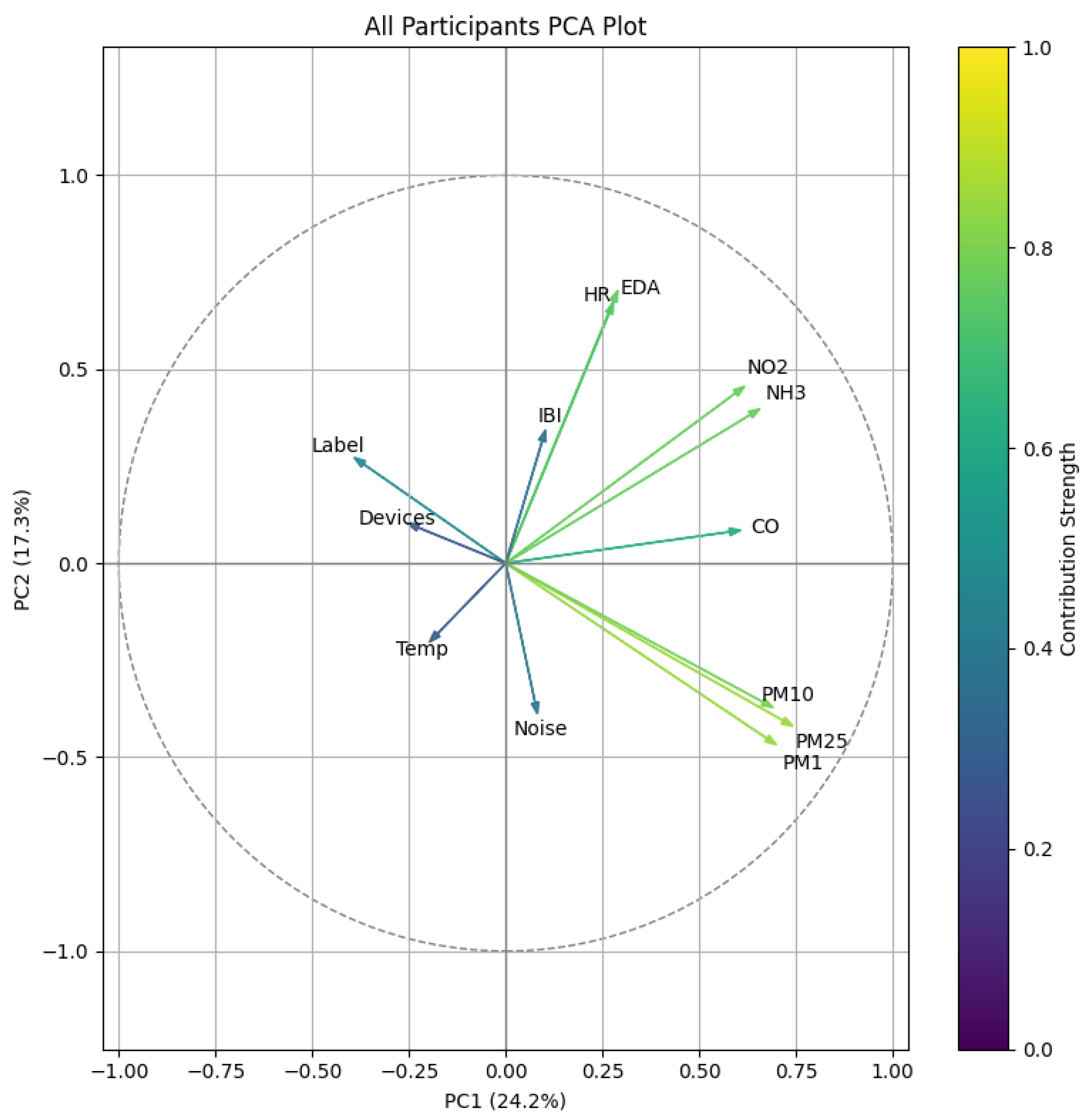
To ascertain the relationship between all variables, we plot the environmental variables (PM1, PM2.5, PM10, NO2, CO, NH3, Noise, Temperature, Number of Nearby Devices), physiological variables (HR, EDA, IBI) and the self-reported label (wellbeing). In Figure 2, principal component (PC) 1 is 24.2%, and PC2 is 17.3% and thus gives a total combined variance of 41.5%. The variance is decreased by the wellbeing label being moderately negatively correlated with PM, indicated by their angle of 180°. The colour scale indicates those variables coloured blue (Noise, Temp, Devices, Label, IBI), which indicate low correlation, and those with yellow (PM1, PM2.5, PM10, NO2, CO, NH3, HR, EDA) indicate a higher degree of correlation.
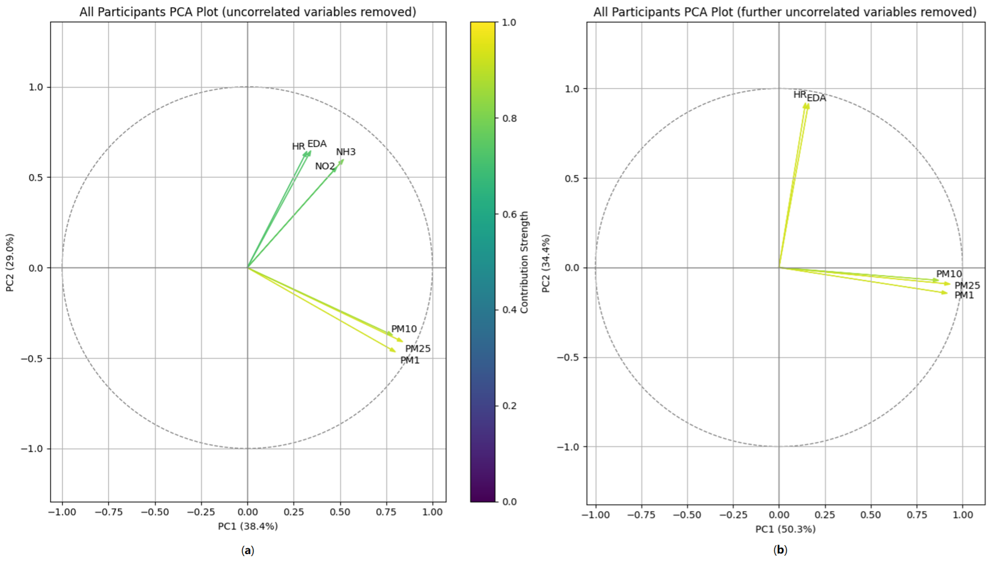
To initially increase variance and therefore the total degree of correlation, variables with a contribution strength of <0.6 were removed. Previous work has shown that values recorded above 0.6 indicate stronger correlations, compared with those lower than 0.6 [53,54]. As a result, depicted at Figure 3, the removal of Noise, Devices, Temp, IBI, label and CO generated a combined total variance of 67.4%. Further removal of NH3 and NO2 increased this total to 84.7% in Figure 3b. The percentage total variance can be used to assess the degree of association between the variables in combination with their angle of proximity [55]. This indicates potential correlations between NH3, NO2 and all three sizes of PM against EDA and HR. The increase to 84.7% with the further removal of NH3 and NO2 suggests that PM has the greatest effect on HR and EDA and through inference the greatest impact on the participants’ wellbeing. The negative correlation between label and PM also suggests that PM has the greatest impact on mental wellbeing. This conclusion aligns with the previous work [46].
The high combined variance of 84.7% when analysing HR and EDA against PM suggests a correlation between environmental PM concentration and HR. The self-reported wellbeing label is also at 180 degrees to PM, indicating it is the group of pollutants having the greatest impact on wellbeing. Consistent with Section 5.2 of our prior work [46], the interpretations presented here are supported by previously published regression and correlation analyses carried out on the same dataset.

3.2. Visualising Spatially Using Heatmaps

Following the results from the PCA, in this section we explore how each of the physiological data variables are individually affected by each of the pollutants through the use of heatmap spatial overlays.

3.2.1. Identifying the Most Suitable Marker for Mental Wellbeing

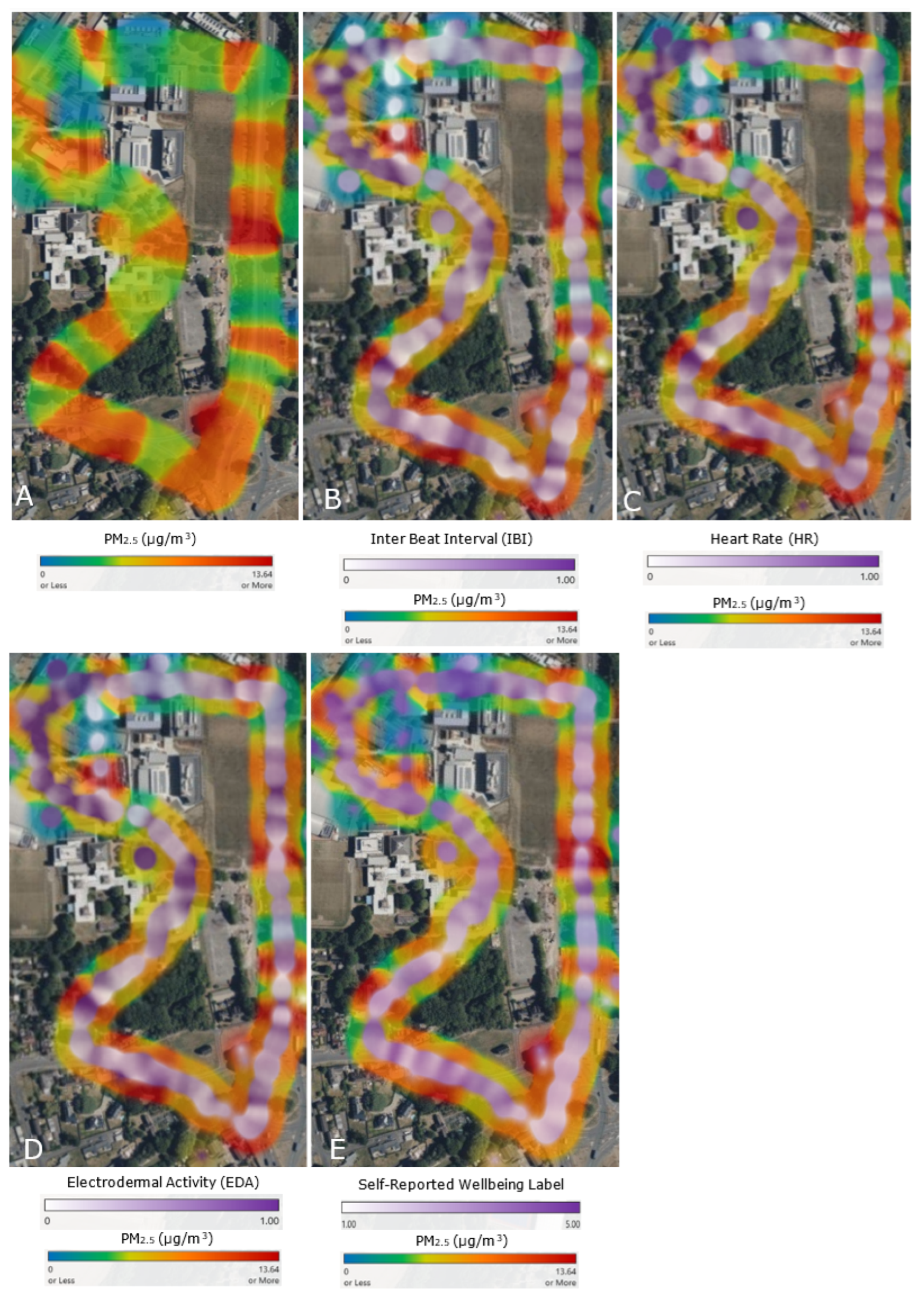
To better understand the most appropriate marker for estimating mental wellbeing, five heatmaps were generated with the bottom layer being PM2.5 concentration (μg/m3) and the second layer being the physiological variables and self-reported wellbeing label. For this section, we selected 10 participants from the DigitalExposome dataset using random sampling. While the full dataset comprises of 40 individuals, the subset was chosen to enable individual-focused, high-resolution analysis of spatial–temporal wellbeing patterns and pollutant exposure effects. The decision reflects both methodological and practical considerations, including computational feasibility and the need for detailed multivariate and spatial analysis. The aim was to establish which variable was the most affected by the fluctuations in PM2.5 concentration and therefore would be the most reliable indicator of the participant’s mental wellbeing. These visualisations can be seen in Figure 4.
Figure 4 illustrates the changes to the three physiological markers and the self-reported wellbeing label as participants walk the designated route. As physiological data was already normalised, scales are depicted as 0–1 where 0 is the individual participants’ lowest points and 1 being their highest. The three physiological markers moderately correlate with each other, for instance sharing high points, particularly in the top left where some of the lowest PM2.5 concentrations were observed. They do however show little correlation with PM2.5 indicating a lack of immediate effect.
The self-reported label correlates far more strongly with PM2.5 and displays a negative correlation. Points of interest are along the A453 carriageway and the entrance to campus along the top. Along the A453, where PM2.5 concentrations are at their highest, wellbeing is generally lower except for one point where the PM2.5 concentration temporarily decreases. Wellbeing then reduced as the higher PM2.5 concentration returns. In contrast, the entrance to campus at the top of the map has some of the lowest PM2.5 concentrations and is reflected by an increase in wellbeing.

3.2.2. Correlating Wellbeing High and Low Spots with PM2.5 Concentration

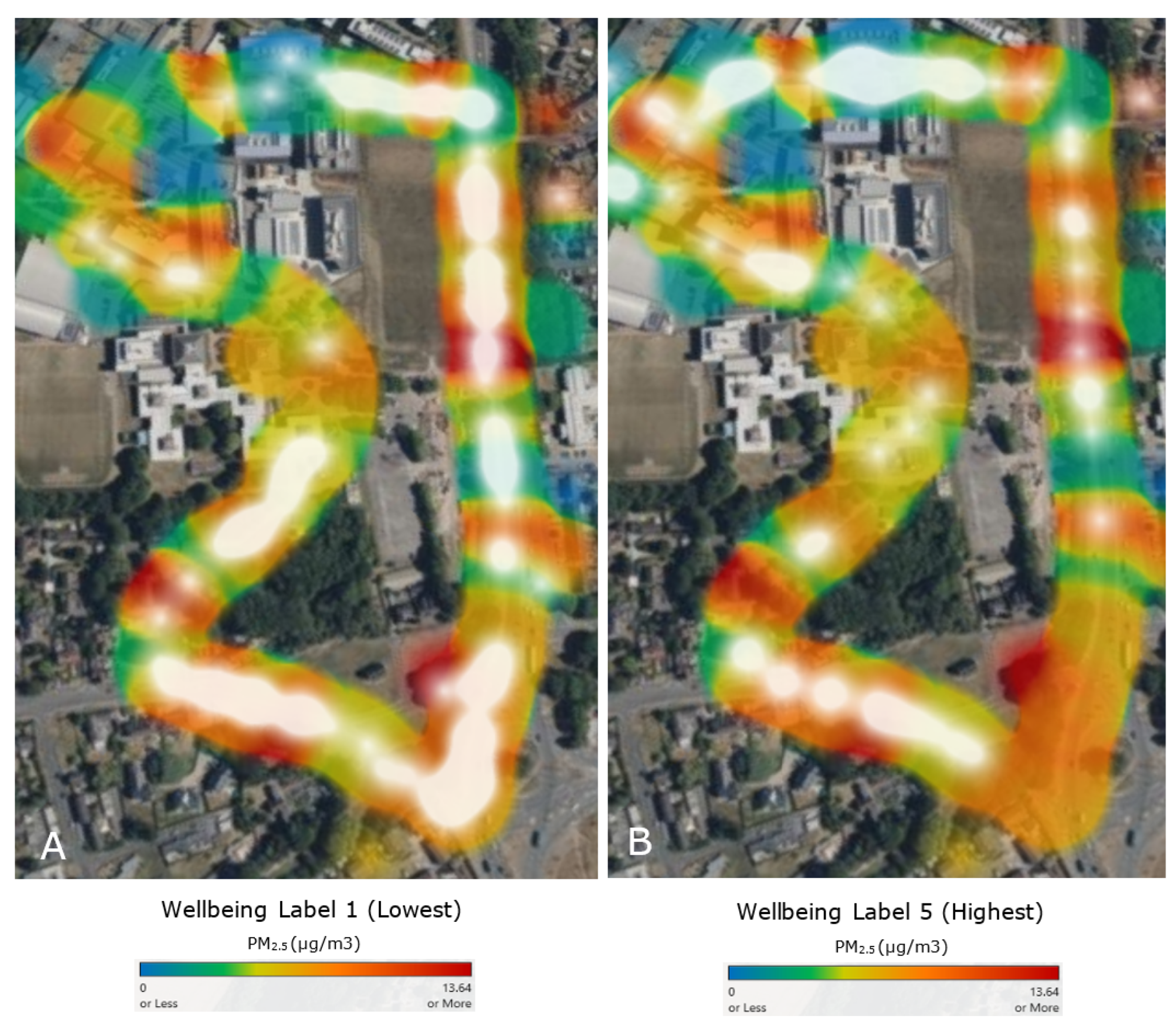
Figure 5 further illustrates the negative correlation between PM2.5 and wellbeing. This is highlighting that, as PM2.5 concentration increases, the level of wellbeing decreases negatively.
The areas where concentrations are at their highest feature the majority of the data points where participants rated their wellbeing the lowest value of 1. Additionally, the areas towards the top of the map featuring the lowest concentrations also contains the majority of the points where participants rated their wellbeing the maximum score of 5. As a result, the self-reported wellbeing marker will be used in the subsequent visualisations to quantify participant mental wellbeing. The remaining pollutants will be ranked by their impact, but PM2.5 will be focused on for the hotspot analysis due to having the greatest impact.

3.2.3. Determining the Remaining Pollutants’ Impact to Mental Wellbeing

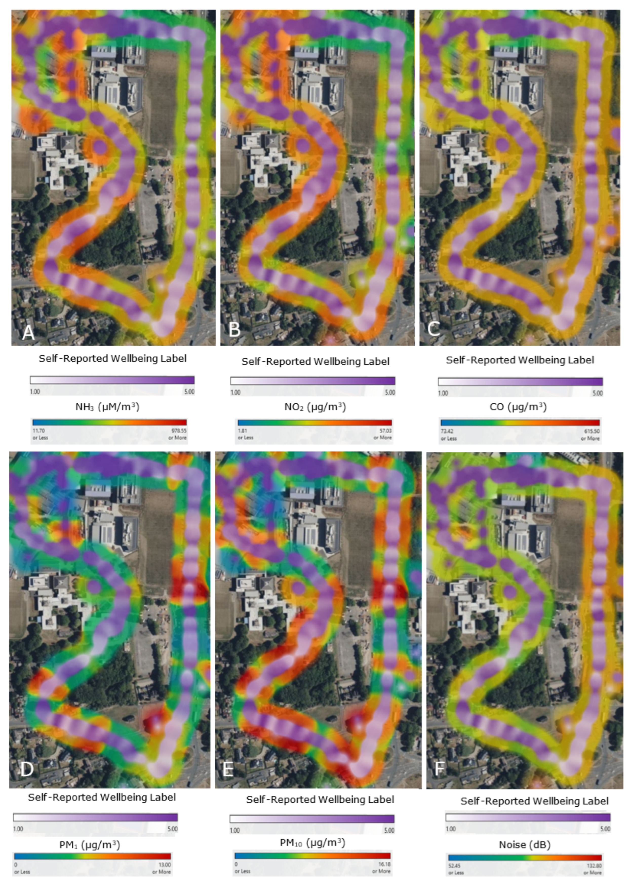
Figure 6 depicts six heatmaps of the pollutants measured along the participant route which includes: NH3 (A), NO2 (B), CO (C), PM2.5 (D), PM10 (E) and Noise (F). To explore the relationship between the participants’ wellbeing and each pollutant, we overlaid their wellbeing label (ranging from 1 to 5) onto each pollutants’ concentration map along the walking routes. This visual integration enables a spatial comparison between perceived wellbeing and environmental exposure. The pollutants are presented in Figure 6 from top left to bottom right in order of their estimated increasing impact on mental wellbeing, based on the prior literature and preliminary analysis.
The nitrogen-based pollutants NH3 and NO2 display the lowest impact with high wellbeing being recorded in areas of both high and low concentrations. This is in spite of the fact NH3 had the highest observed average concentrations of all the pollutants, for instance when compared to PM2.5, NH3 had an average concentration of 325 μmol/m3 where as PM2.5 was only 6 μg/m3. Both pollutants have low points along the roadside at the right of the map, but this is not reflected in the participant’s self-reported wellbeing. The wellbeing labels of 5 are more often situated in areas of higher concentrations of both NO2 and NH3, suggesting negligible negative impact to mental wellbeing.
CO displayed one of the most consistent concentrations of all the pollutants. The area of lowest observed concentration correlates with the other pollutants at the top centre of the route that contained green spaces. This consistency in concentration makes it difficult to assess how changes in concentration affect mental wellbeing, but due to the vast array of different wellbeing responses, other pollutants have a stronger correlation.
PM1 and PM10 display similar concentration patterns but since PM1 excludes matter with a particle size larger than 1 μm and PM10 larger than 10 μm, PM1 has lower overall concentrations and fewer hotspots. Both show the highest concentrations at the roadside, but both have the lowest concentrations of any pollutant in Figure 6. Despite this, there is a higher degree of correlation with participant wellbeing compared to the previously discussed pollutants. Wellbeing is lower in all of the hotspots for both sizes of PM but the higher frequency of PM10 hotspots yields a greater impact to mental wellbeing compared to PM1 in this data.

3.2.4. Comparing the Influence of Noise to Pollution on Mental Wellbeing

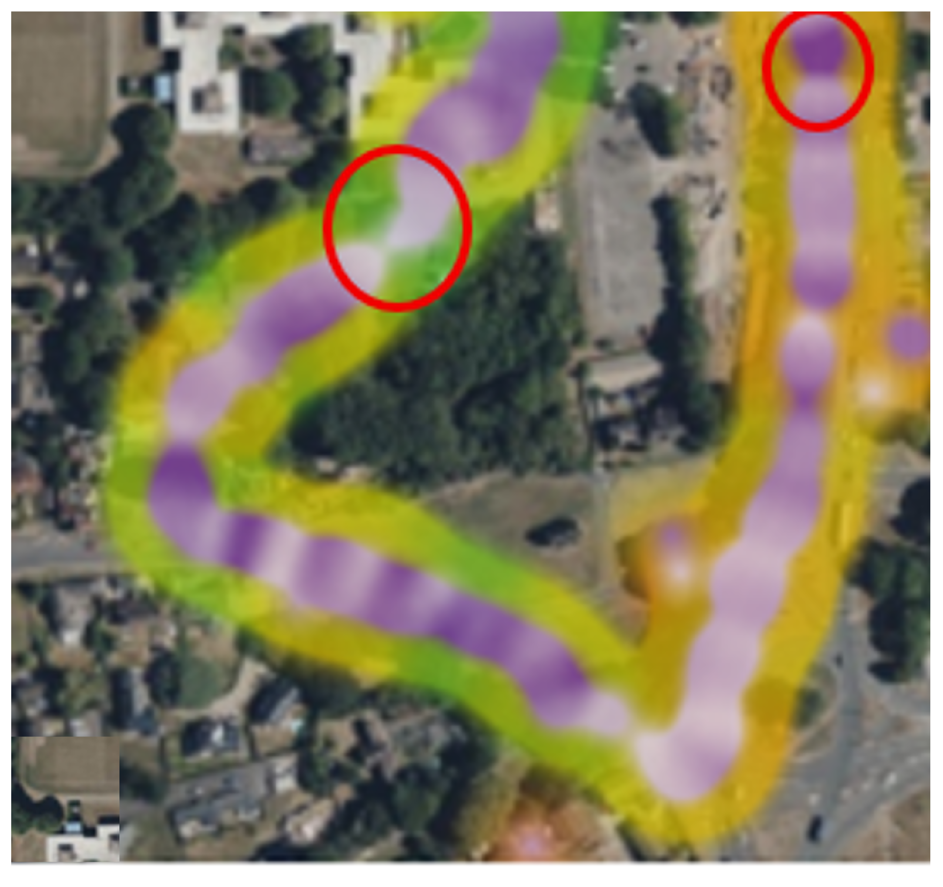
For comparison, noise was also mapped with wellbeing overlayed. As expected, noise was consistently higher by the roadside, with the highest levels observed towards the top of the road. The lowest noise levels correlate with the lowest concentrations of the other pollutants at the top centre of the route. As noise levels increase, wellbeing generally decreases, which is in line with other findings and previous work [47]. It is worth noting that, by exploring this work further, wellbeing is impacted by more than just noise as depicted in Figure 7.
The circle (left in Figure 7) sees a significant drop in wellbeing (5 to 1), just as noise levels also drop. This point is demonstrated in both Figure 4 and Figure 6 to be an exact hotspot for both PM2.5 and PM10. The circle (right in Figure 7) at this point indicates a temporary increase in reported wellbeing, which does not correspond with a reduction in noise levels. Instead, it coincides with a brief decrease in Particulate Matter (PM) concentrations. Subsequently, as PM levels return to their prior concentrations, a rapid decline in wellbeing is observed. This pattern highlights the temporal sensitivity of wellbeing to air quality fluctuations; the alignment between changes in PM levels and wellbeing suggests a short-term responsiveness in participants’ perceptions.
Additionally, a comparison between noise and PM2.5 indicates that PM2.5 displays a more focused spatial and temporal association with wellbeing. Noise levels fluctuate sharply due to short-lived environmental events (e.g., passing vehicles), PM2.5 concentrations vary more gradually across the route. This stability means that changes in wellbeing align more reliably with PM2.5 hotspots, whereas noise demonstrates a weaker and less predictable relationship with momentary wellbeing.

3.3. Visualising PM2.5 Hotspots Using Voronoi Display

As PM2.5 has been previously identified as having the greatest impact on the participants’ mental wellbeing, it is important to understand where the hotspots are and how to determine their sources. Voronoi is a widely used technique, renowned for displaying exposures linked to GIS (Geographic Information System) data [46,51]. Compared to the heatmaps, Voronoi Displays are more ideal for identifying hotspots as each data point is represented by its own, coloured polygon. Comparatively, heatmaps average out the data points so can obscure hotspots, particularly if they only occur in a limited number of participants.
To facilitate comparison between visualisation techniques, the same participants from the DigitalExposome dataset that were used to generate the heatmaps were used to produce a Voronoi Display of the PM2.5 concentrations. This offers an alternate perspective as each data point has its own unique polygon square instead featuring a blending of all the data points.
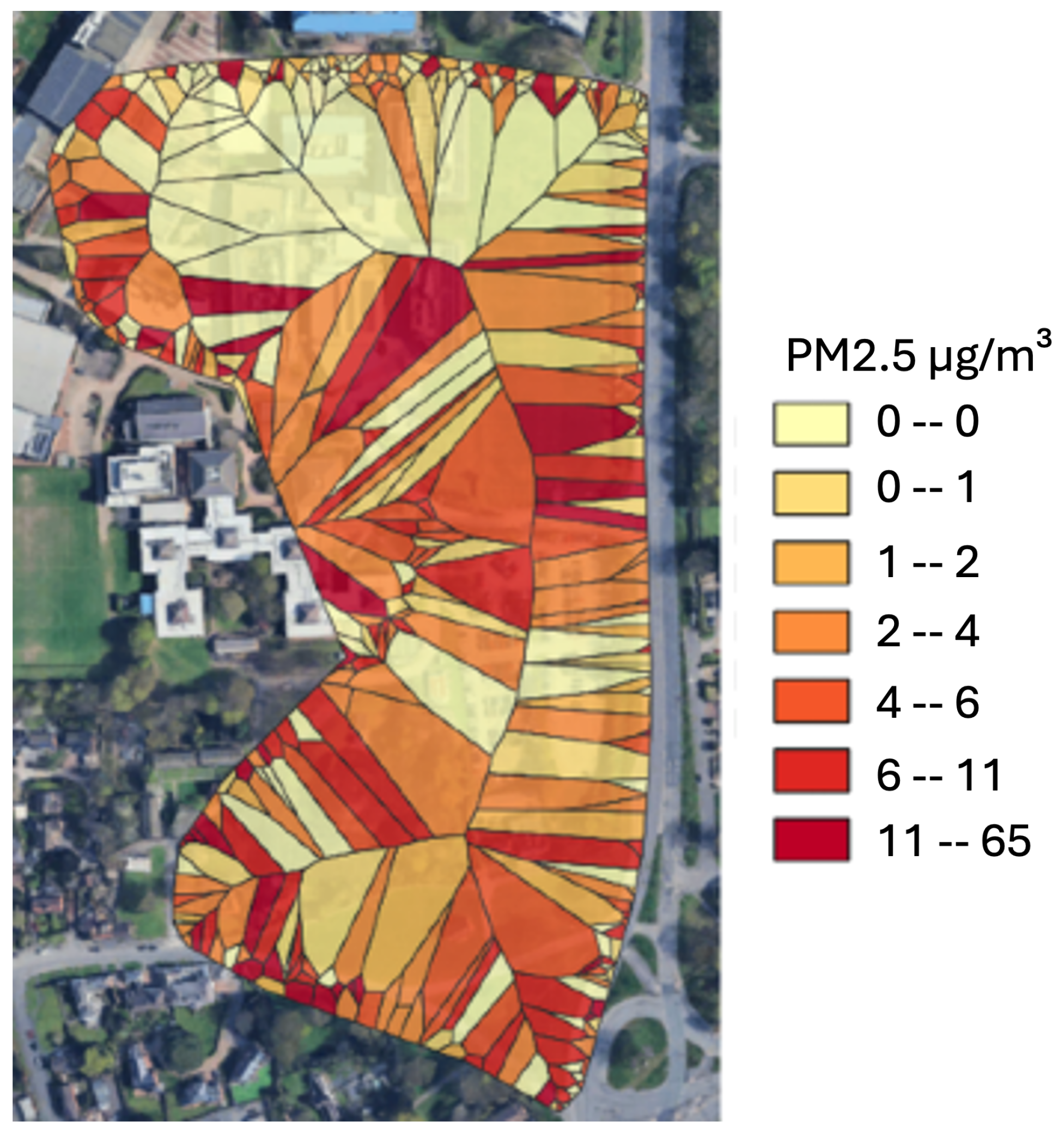
Figure 8 illustrates the PM2.5 pollution concentrations (μg/m3) along the participant’s walking route with interpolations of the internal campus concentrations. Although this allows for a direct comparison of the same data visually different from Figure 6A, it highlights a potential drawback of applying Voronoi to datasets that contain a large number of overlapping data points. This results from each data point having its own, coloured polygon, so overlapping data points lead to several small polygons being generated next to each other that are often hard to interpret visually.

Visualising a Singular Participant with Voronoi

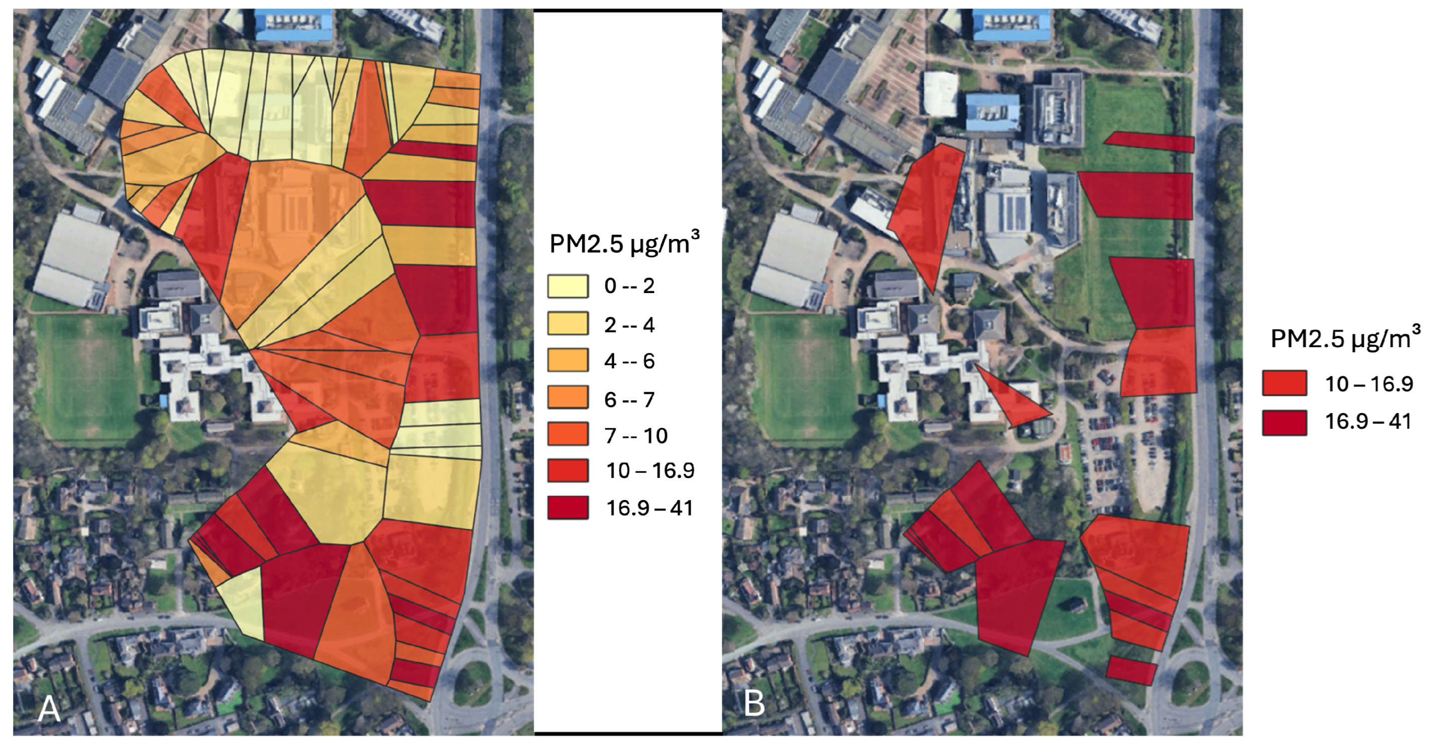
To overcome this limitation, a single participant was selected at random from the dataset, and their PM2.5 data was used to produce two new Voronoi Displays that could be used to more accurately identify pollution hotspots, as depicted at Figure 9.
Figure 9 presents a clearer visualisation when compared to Figure 8 by having a more consistent polygon size. The data can be interpreted similarly to the heatmaps, but the individual hotspots can be seen far more easily. The hotspots along the road to the right were to be expected but unexpectedly there is a hotspot situated on the campus near the top left of the figure. This hotspot was somewhat visible on the heatmaps but is far clearer on Figure 9. This highlights that Voronoi can be used to identify pollution hotspots as well as predict pollution concentrations via spatial partitioning, illustrated by the polygons inside the walking route.

4. Discussion

PM2.5 was found to have the most significant impact on the participants’ mental wellbeing, as revealed through Principal Component Analysis (PCA). This finding corroborates results from previous work [46] and aligns with the broader literature, including studies linking PM10 exposure to reduced life satisfaction and wellbeing [56] and PM2.5 being identified as the most influential pollutant on mental health outcomes [57].
The spatial representation of PM2.5 concentrations via heatmaps enabled comparative analysis against physiological variables and self-reported wellbeing labels. While physiological indicators such as Inter-Beat Interval (IBI) and Electrodermal Activity (EDA) showed some sensitivity to elevated PM2.5 levels, the self-reported wellbeing label demonstrated a stronger and more consistent correlation. This suggests its potential utility as a robust and scalable marker of environmental stress, particularly when physiological data is limited or short-term exposure is being assessed, as demonstrated in our earlier work [58]. The current study extends this concept by showing that self-reported wellbeing labels not only correlate more strongly with environmental stressors like PM2.5 but also offer a scalable and interpretable metric for urban health monitoring. This reinforces the argument that subjective wellbeing, when captured systematically, can serve as a reliable proxy for environmental stress; particularly in scenarios where physiological data may be limited by temporal or technical constraints.
Previous research has demonstrated the correlation between PM2.5 concentration and reduced IBI [59]. The physiological effects are understood to be cumulative [60], with sustained exposures of 4–6 h producing significant observable changes [61]. Despite participants in this study being exposed for only 40 min, weak correlations were still observed between the pollutants and the physiological variables, demonstrating the utility of this type of data analysis. This supports the use of self-reporting wellbeing as the primary data collection methodology in short-duration studies. This does provide scope; however, it also reperforms the data collection in longer term studies.
Figure 4 and Figure 5 illustrate the spatial distribution of wellbeing scores, with lower scores predominantly observed roadside and higher scores near green spaces. This generally correlates negatively with PM2.5 concentrations, though some contradictory points exist, particularly at the bottom of the map where both low and high wellbeing scores overlap. These anomalies may be attributed to external factors such as traffic variability or subjective rating inconsistencies [62].
Noise levels ranged from 47 dB to 120 dB, with higher levels recorded alongside the roadside compared to pedestrianised campus areas. A negative correlation between noise and wellbeing was observed (Figure 6F), which is consistent with prior research [63]. Also, increasing noise from 60 dB to 100 dB accelerates stress onset from 25 min to less than 5 min [64]. However, there remains a lack of the literature investigating immediate changes in mental wellbeing resulting from noise levels. Our results, at some data points show a contradiction, whereby wellbeing positively correlates with noise, suggesting that noise may not be the sole influencing factor. These instances do coincide with PM2.5 hotspots and low concentrations, reinforcing the hypothesis that PM2.5 may exert a stronger influence on wellbeing than noise.
Comparing the impacts of both PM2.5 and noise, PM2.5 demonstrates a more consistent negative association with momentary wellbeing than noise. Specifically, in this work we explore how PM2.5 varies gradually and forms spatially coherent hotspots that align closely with low wellbeing labels, indicating that higher PM2.5 causes a reduced wellbeing in urban environments. On the other hand, noise levels fluctuate rapidly between 47–120 dB due to moving events such as passing vehicles. These contrasting temporal dynamics help explain why wellbeing tracks PM2.5 more reliably, the stable variation in PM2.5 provides a stronger short-term signal, while the high-frequency volatility of noise produces irregular and often weaker correspondence with wellbeing.
Voronoi visualisations have provided valuable insight into how environmental changes can influence mental wellbeing. By assigning unique polygons to each data point, this method avoids the averaging seen in heatmaps and preserves spatial granularity. When applied to PM2.5 from the DigitalExposome dataset, Voronoi diagrams offered an alternate perspective on pollution distribution.
The results demonstrate that we can identify pollutant hotspots and predict concentrations in surrounding areas, as depicted at Figure 9B. While group-level Voronoi visualisations offered a useful overview of PM2.5 distribution, they also revealed a limitation: overlapping data points resulted in numerous small polygons that were difficult to interpret. To address this, a single participant’s data was visualised separately, producing clearer and more consistent polygon sizes.
Figure 9 shows this refined view, where pollution hotspots especially one location within the university campus were more easily identifiable. This supports the use of Voronoi visualisation for detecting localised environmental stressors and predicting pollutant concentrations. These findings demonstrate that Voronoi-based spatial analysis can effectively highlight areas of environmental concern and their potential impact on mental wellbeing. Typically, areas with elevated PM2.5 concentrations corresponded with lower self-reported wellbeing scores, consistent with previous studies [65,66]. Moreover, this form of spatial partitioning helps assess the degree to which a location resembles its surroundings, offering a scalable tool for urban health monitoring and environmental planning.

5. Conclusions and Future Work

This paper has demonstrated the utility of both heatmaps and Voronoi diagrams as effective tools for exploring the relationship between environmental pollutants and mental wellbeing. These visualisation techniques enabled the identification of pollutant-specific spatial patterns and individual-level exposure hotspots, offering a more nuanced understanding of how urban environmental stressors affect psychological states. The analysis was conducted using data from the DigitalExposome dataset, in which 40 participants walked a predefined urban route while carrying environmental and physiological sensors and reporting their momentary wellbeing.
The findings align with previous research, confirming that PM2.5 is the pollutant most strongly associated with negatively impacted mental wellbeing. However, this study extends earlier work by proposing a preliminary ranking of other pollutants based on their individual impacts and by comparing the relative influence of noise versus air pollution. The introduction of Voronoi Display as a spatial analysis method also offers a novel approach to identifying pollution hotspots and their potential psychological implications.
These results have broader implications for urban planning and public health. By visualising pollutant impact at multiple spatial levels, this work supports the development of targeted interventions; such as the strategic placement of green spaces or traffic re-routing—to mitigate environmental stressors in high-risk areas. Furthermore, the integration of physiological and self-reported data provides a more ecologically valid framework for assessing mental wellbeing in real-world settings.
Despite these contributions, this study has some limitations in the further exploration of visualisation techniques which may yield additional insights. For example, representing heatmaps using bar plots or multi-angle perspectives could enhance interpretability and reveal hidden patterns. Longitudinal data collection and cross-city comparisons would also help assess cumulative exposure effects and urban disparities. Ultimately, these approaches can contribute to a deeper understanding of how environmental conditions shape mental wellbeing and inform evidence-based urban design strategies.

Author Contributions

Author contributions: conceptualization, Morgan Ecclestone and Thomas Johnson; methodology, Morgan Ecclestone and Thomas Johnson; software, Morgan Ecclestone; validation, Morgan Ecclestone and Thomas Johnson; formal analysis, Morgan Ecclestone; investigation, Morgan Ecclestone and Thomas Johnson; resources, Thomas Johnson; data curation, Thomas Johnson; writing—original draft preparation, Morgan Ecclestone and Thomas Johnson; writing—review and editing, Morgan Ecclestone and Thomas Johnson; visualization, Morgan Ecclestone; supervision, Thomas Johnson. All authors have read and agreed to the published version of the manuscript.

Funding

This research received no external funding.

Data Availability Statement

The dataset will be provided upon request or can be downloaded via Mendeley [67].

Conflicts of Interest

The authors declare there are no conflicts of interest.

Abbreviations

The following abbreviations are used in this manuscript:
EMAEcological Momentary Assessment
BVPBlood Volume Pulse
IBIInter-Beat Interval
COPDChronic Obstructive Pulmonary Disorder
EDAElectrodermal Activity
PMParticulate Matter
COCarbon Monoxide
GISGeographic Information System
NO2Nitrogen Dioxide
NH3Ammonia
WHOWorld Health Organisation
PCAPrincipal Component Analysis

References

  1. Guite, H.F.; Clark, C.; Ackrill, G. The impact of the physical and urban environment on mental well-being. Public Health 2006, 120, 1117–1126. [Google Scholar] [CrossRef]
  2. Johnson, T.; Kanjo, E. Sensor Fusion and The City: Visualisation and Aggregation of Environmental & Wellbeing Data. In Proceedings of the 2021 IEEE International Smart Cities Conference (ISC2), Manchester, UK, 7–10 September 2021. [Google Scholar] [CrossRef]
  3. WHO. Air Quality, Energy and Health. 2024. Available online: https://www.who.int/teams/environment-climate-change-and-health/air-quality-energy-and-health (accessed on 19 March 2026).
  4. Marais, E.A.; Vohra, K.; Kelly, J.M.; Li, Y.; Lu, G. The health burden of air pollution in the UK: A modelling study using updated exposure-risk associations. Lancet 2023, 402, S66. [Google Scholar] [CrossRef] [PubMed]
  5. Bakolis, I.; Hammoud, R.; Stewart, R.; Beevers, S.; Dajnak, D.; MacCrimmon, S.; Broadbent, M.; Pritchard, M.; Shiode, N.; Fecht, D.; et al. Mental health consequences of urban air pollution: Prospective population-based longitudinal survey. Soc. Psychiatry Psychiatr. Epidemiol. 2021, 56, 1587–1599. [Google Scholar] [CrossRef] [PubMed]
  6. Newbury, J.B.; Stewart, R.; Fisher, H.L.; Beevers, S.; Dajnak, D.; Broadbent, M.; Pritchard, M.; Shiode, N.; Heslin, M.; Hammoud, R.; et al. Association between air pollution exposure and mental health service use among individuals with first presentations of psychotic and mood disorders: Retrospective cohort study. Br. J. Psychiatry 2021, 219, 678–685. [Google Scholar] [CrossRef]
  7. Analitis, A.; Katsouyanni, K.; Dimakopoulou, K.; Samoli, E.; Nikoloulopoulos, A.K.; Petasakis, Y.; Touloumi, G.; Schwartz, J.; Anderson, H.R.; Cambra, K.; et al. Short-term effects of ambient particles on cardiovascular and respiratory mortality. Epidemiology 2006, 17, 230–233. [Google Scholar] [CrossRef]
  8. Pryor, J.T.; Cowley, L.O.; Simonds, S.E. The Physiological Effects of Air Pollution: Particulate Matter, Physiology and Disease. Front. Public Health 2022, 10, 882569. [Google Scholar] [CrossRef] [PubMed]
  9. Ji, S.; Guo, Y.; Yan, W.; Wei, F.; Ding, J.; Hong, W.; Wu, X.; Ku, T.; Yue, H.; Sang, N. PM2.5 exposure contributes to anxiety and depression-like behaviors via phenyl-containing compounds interfering with dopamine receptor. Proc. Natl. Acad. Sci. USA 2024, 121, e2319595121. [Google Scholar] [CrossRef]
  10. Kunay, B.; Yılmaz, Ö.; Yüksel, H. Emergency Admissions Due to Respiratory Problems in Children Change with Extend of Air Pollution. J. Pediatr. Res. 2025, 12, 83–89. [Google Scholar] [CrossRef]
  11. Chauhan, A.J.; Inskip, H.M.; Linaker, C.H.; Smith, S.; Schreiber, J.; Johnston, S.L.; Holgate, S.T. Personal exposure to nitrogen dioxide (NO2) and the severity of virus-induced asthma in children. Lancet 2003, 361, 1939–1944. [Google Scholar] [CrossRef]
  12. Zhang, P.; Arora, M.; Chaleckis, R.; Isobe, T.; Jain, M.; Meister, I.; Melén, E.; Perzanowski, M.; Torta, F.; Wenk, M.R.; et al. Tackling the complexity of the exposome: Considerations from the gunma university initiative for advanced research (GIAR) exposome symposium. Metabolites 2019, 9, 106. [Google Scholar] [CrossRef]
  13. Hampson, N.B. Carbon monoxide poisoning mortality in the United States from 2015–2021. Clin. Toxicol. 2023, 61, 483–491. [Google Scholar] [CrossRef] [PubMed]
  14. Donzelli, G.; Suarez-Varela, M.M. Tropospheric Ozone: A Critical Review of the Literature on Emissions, Exposure, and Health Effects. Atmosphere 2024, 15, 779. [Google Scholar] [CrossRef]
  15. Münzel, T.; Gori, T.; Babisch, W.; Basner, M. Cardiovascular effects of environmental noise exposure. Eur. Heart J. 2014, 35, 829–836. [Google Scholar] [CrossRef]
  16. Urban Population Division. Urban Population (% of Total Population)—United Kingdom|Data. 2024. Available online: https://www.un.org/development/desa/pd/sites/www.un.org.development.desa.pd/files/undesa_pd_2024_wpp_2024_advance_unedited_0.pdf (accessed on 19 March 2026).
  17. Zhong, J.; Stocker, J.; Cai, X.; Harrison, R.M.; Bloss, W.J. Street-scale air quality modelling over the West Midlands, United Kingdom: Effect of idealised traffic reduction scenarios. Urban Clim. 2024, 55, 101961. [Google Scholar] [CrossRef]
  18. Brunt, H.; Barnes, J.; Jones, S.J.; Longhurst, J.W.; Scally, G.; Hayes, E. Air pollution, deprivation and health: Understanding relationships to add value to local air quality management policy and practice in Wales, UK. J. Public Health 2017, 39, 485–497. [Google Scholar] [CrossRef]
  19. Horton, A.; Jones, S.J.; Brunt, H. Air pollution and public health vulnerabilities, susceptibilities and inequalities in Wales, UK. J. Public Health 2023, 45, 432–441. [Google Scholar] [CrossRef] [PubMed]
  20. Boningari, T.; Smirniotis, P.G. Impact of nitrogen oxides on the environment and human health: Mn-based materials for the NOx abatement. Curr. Opin. Chem. Eng. 2016, 13, 133–141. [Google Scholar] [CrossRef]
  21. Carnell, C.; Vieno, M.; Vardoulakis, S.; Beck, R.; Tomlinsonc, S.; Dragosits, U.; Heal, M.R.; Reis, S. Modelling public health improvements as a result of air pollution control policies in the UK over four decades—1970 to 2010. Environ. Res. Lett. 2019, 14, 074001. [Google Scholar] [CrossRef]
  22. Wild, C.P. Complementing the genome with an “exposome”: The outstanding challenge of environmental exposure measurement in molecular epidemiology. Cancer Epidemiol. Biomarkers Prev. 2005, 14, 1847–1850. [Google Scholar] [CrossRef]
  23. Wild, C.P. The exposome: From concept to utility. Int. J. Epidemiol. 2012, 41, 24–32. [Google Scholar] [CrossRef] [PubMed]
  24. Moore, T.M.; Visoki, E.; Argabright, S.T.; Didomenico, G.E.; Sotelo, I.; Wortzel, J.D.; Naeem, A.; Gur, R.C.; Gur, R.E.; Warrier, V.; et al. Modeling environment through a general exposome factor in two independent adolescent cohorts. Exposome 2022, 2, osac010. [Google Scholar] [CrossRef]
  25. Bhui, K.; Newbury, J.B.; Latham, R.M.; Ucci, M.; Nasir, Z.A.; Turner, B.; O’leary, C.; Fisher, H.L.; Marczylo, E.; Douglas, P.; et al. Air quality and mental health: Evidence, challenges and future directions. BJPsych Open 2023, 9, e120. [Google Scholar] [CrossRef]
  26. Padhy, S.K.; Sarkar, S.; Davuluri, T.; Patra, B.N. Urban living and psychosis—An overview. Asian J. Psychiatry 2014, 12, 17–22. [Google Scholar] [CrossRef]
  27. Finnemann, A.; Skjerdingstad, N.; Speyer, L.G.; Zavlis, O.; Bartoš, F.; Wiers, R.; van der Maas, H.; Sibley, C.G.; Johnson, S.U.; Helmich, M.A.; et al. Urban-rural differences in anxiety and depression in the UK, New Zealand, and Norway. J. Affect. Disord. 2025, 388, 119601. [Google Scholar] [CrossRef]
  28. Lin, J.; Feng, S.T.; Wu, Z.Y.; Dong, L.R.; Yin, D.Q.; Zhu, H.; Jia, H.X.; Ning, Y.Z. Interaction between the brain and multiple organ systems in schizophrenia. World J. Psychiatry 2025, 15, 107696. [Google Scholar] [CrossRef] [PubMed]
  29. Baker, E.; Barlow, C.F.; Daniel, L.; Morey, C.; Bentley, R.; Taylor, M.P. Mental health impacts of environmental exposures: A scoping review of evaluative instruments. Sci. Total Environ. 2024, 912, 169063. [Google Scholar] [CrossRef] [PubMed]
  30. Russo, R.C.; Togbe, D.; Couillin, I.; Segueni, N.; Han, L.; Quesniaux, V.F.; Stoeger, T.; Ryffel, B. Ozone-induced lung injury and inflammation: Pathways and therapeutic targets for pulmonary diseases caused by air pollutants. Environ. Int. 2025, 198, 109391. [Google Scholar] [CrossRef] [PubMed]
  31. King, J.D.; Zhang, S.; Cohen, A. Air pollution and mental health: Associations, mechanisms and methods. Curr. Opin. Psychiatry 2022, 35, 192–199. [Google Scholar] [CrossRef]
  32. Gao, N.; Rahaman, M.S.; Shao, W.; Salim, F.D. Investigating the Reliability of Self-report Data in the Wild: The Quest for Ground Truth. In UbiComp/ISWC 2021—Adjunct Proceedings of the 2021 ACM International Joint Conference on Pervasive and Ubiquitous Computing and Proceedings of the 2021 ACM International Symposium on Wearable Computers; ACM: New York, NY, USA, 2021; pp. 237–242. [Google Scholar] [CrossRef]
  33. Black, J.T.; Shakir, M.Z. Emotion on the edge: An evaluation of feature representations and machine learning models. Nat. Lang. Process. J. 2025, 10, 100127. [Google Scholar] [CrossRef]
  34. Whyte, C.; O’Toole, M.D.; Casson, A.J.; Gowen, E. A Feasibility Study of Data Driven Ecological Momentary Assessment Surveys Using Smart Wearables to Capture Emotions. In 2024 IEEE Sensors Applications Symposium, SAS 2024—Proceedings; IEEE: Piscataway, NJ, USA, 2024. [Google Scholar] [CrossRef]
  35. de Vries, L.P.; Baselmans, B.M.; Bartels, M. Smartphone-Based Ecological Momentary Assessment of Well-Being: A Systematic Review and Recommendations for Future Studies. J. Happiness Stud. 2021, 22, 2361–2408. [Google Scholar] [CrossRef]
  36. Ueberham, M.; Schlink, U. Wearable sensors for multifactorial personal exposure measurements—A ranking study. Environ. Int. 2018, 121, 130–138. [Google Scholar] [CrossRef]
  37. Matsumura, G.; Honda, S.; Kikuchi, T.; Mizuno, Y.; Hara, H.; Kondo, Y.; Nakamura, H.; Watanabe, S.; Hayakawa, K.; Nakajima, K.; et al. Real-time personal healthcare data analysis using edge computing for multimodal wearable sensors. Device 2025, 3, 100597. [Google Scholar] [CrossRef]
  38. Mao, Y.; You, C.; Zhang, J.; Huang, K.; Letaief, K.B. A Survey on Mobile Edge Computing: The Communication Perspective. IEEE Commun. Surv. Tutor. 2017, 19, 2322–2358. [Google Scholar] [CrossRef]
  39. Johnson, T.; Kanjo, E. Urban Wellbeing: A Portable Sensing Approach to unravel the link between Environment and Mental Wellbeing. IEEE Sens. Lett. 2023, 7, 5500704. [Google Scholar] [CrossRef]
  40. Stinson, L.; Liu, Y.; Dallery, J. Ecological Momentary Assessment: A Systematic Review of Validity Research. Perspect. Behav. Sci. 2022, 45, 469–493. [Google Scholar] [CrossRef] [PubMed]
  41. Tutunji, R.; Kogias, N.; Kapteijns, B.; Krentz, M.; Krause, F.; Vassena, E.; Hermans, E.J. Detecting Prolonged Stress in Real Life Using Wearable Biosensors and Ecological Momentary Assessments: Naturalistic Experimental Study. J. Med. Internet Res. 2023, 25, e39995. [Google Scholar] [CrossRef]
  42. Morgiève, M.; Genty, C.; Azé, J.; Dubois, J.; Leboyer, M.; Vaiva, G.; Berrouiguet, S.; Courtet, P. A Digital Companion, the Emma App, for Ecological Momentary Assessment and Prevention of Suicide: Quantitative Case Series Study. JMIR Mhealth Uhealth 2020, 8, e15741. [Google Scholar] [CrossRef]
  43. World’s Air Pollution: Real-Time Air Quality IndexProject. World’s Air Pollution: Real-Time Air Quality Index. 2025. Available online: https://waqi.info/#/c/5.599/7.091/2.8z (accessed on 19 March 2026).
  44. Li, H.; Fan, H.; Mao, F. A Visualization Approach to Air Pollution Data Exploration—A Case Study of Air Quality Index (PM2.5) in Beijing, China. Atmosphere 2016, 7, 35. [Google Scholar] [CrossRef]
  45. Johnson, T. DigitalExposome: A dataset for wellbeing classification using environmental air quality and human physiological data. Data Brief 2025, 59, 111442. [Google Scholar] [CrossRef]
  46. Johnson, T.; Kanjo, E.; Woodward, K. DigitalExposome: Quantifying impact of urban environment on wellbeing using sensor fusion and deep learning. Comput. Urban Sci. 2023, 3, 14. [Google Scholar] [CrossRef]
  47. Kanjo, E.; Younis, E.M.; Sherkat, N. Towards unravelling the relationship between on-body, environmental and emotion data using sensor information fusion approach. Inf. Fusion 2018, 40, 18–31. [Google Scholar] [CrossRef]
  48. Bradley, M.M.; Lang, P.J. Measuring emotion: The self-assessment manikin and the semantic differential. J. Behav. Ther. Exp. Psychiatry 1994, 25, 49–59. [Google Scholar] [CrossRef]
  49. Younis, E.M.; Kanjo, E.; Chamberlain, A. Designing and evaluating mobile self-reporting techniques: Crowdsourcing for citizen science. Pers. Ubiquitous Comput. 2019, 23, 329–338. [Google Scholar] [CrossRef]
  50. Metsalu, T.; Vilo, J. ClustVis: A web tool for visualizing clustering of multivariate data using Principal Component Analysis and heatmap. Nucleic Acids Res. 2015, 43, W566–W570. [Google Scholar] [CrossRef] [PubMed]
  51. Bae, W.D.; Alkobaisi, S.; Meyers, W.; Narayanappa, S.; Vojtechovský, P. Voronoi maps: An approach to individual-based environmental exposure estimation. In Proceedings of the ACM Symposium on Applied Computing; ACM: New York, NY, USA, 2016; pp. 596–603. [Google Scholar] [CrossRef]
  52. Balzer, M.; Deussen, O. Voronoi Treemaps. In Proceedings—IEEE Symposium on Information Visualization, INFO VIS; IEEE: Piscataway, NJ, USA, 2005; pp. 49–56. [Google Scholar] [CrossRef]
  53. MacCallum, R.C.; Widaman, K.F.; Zhang, S.; Hong, S. Sample size in factor analysis. Psychol. Methods 1999, 4, 84–99. [Google Scholar] [CrossRef]
  54. Zhang, N.; Casasent, T.D.; Casasent, A.K.; Kumar, S.V.; Wakefield, C.; Broom, B.M.; Weinstein, J.N.; Akbani, R. PCA-Plus: Enhanced principal component analysis with illustrative applications to batch effects and their quantitation. bioRxiv 2024. [Google Scholar] [CrossRef] [PubMed]
  55. Jollife, I.T.; Cadima, J. Principal component analysis: A review and recent developments. Philos. Trans. R. Soc. A Math. Phys. Eng. Sci. 2016, 374, 20150202. [Google Scholar] [CrossRef]
  56. Petrowski, K.; Bührer, S.; Strauß, B.; Decker, O.; Brähler, E. Examining air pollution (PM10), mental health and well-being in a representative German sample. Sci. Rep. 2021, 11, 18436. [Google Scholar] [CrossRef]
  57. Borroni, E.; Pesatori, A.C.; Bollati, V.; Buoli, M.; Carugno, M. Air pollution exposure and depression: A comprehensive updated systematic review and meta-analysis. Environ. Pollut. 2022, 292, 118245. [Google Scholar] [CrossRef]
  58. Johnson, T.; Woodward, K.; Kanjo, E. Emotion on the Edge: Air Quality Sensors Decoded as a Real-World Emotion Indicator. In 2024 IEEE International Conference on Pervasive Computing and Communications Workshops and other Affiliated Events, PerCom Workshops 2024; IEEE: Piscataway, NJ, USA, 2024; pp. 267–272. [Google Scholar] [CrossRef]
  59. Park, S.K.; O’Neill, M.S.; Vokonas, P.S.; Sparrow, D.; Schwartz, J. Effects of Air Pollution on Heart Rate Variability: The VA Normative Aging Study. Environ. Health Perspect. 2005, 113, 304–309. [Google Scholar] [CrossRef]
  60. Wang, H.; Liu, L. Experimental investigation about effect of emotion state on people’s thermal comfort. Energy Build. 2020, 211, 109789. [Google Scholar] [CrossRef]
  61. He, F.; Shaffer, M.L.; Li, X.; Rodriguez-Colon, S.; Wolbrette, D.L.; Williams, R.; Cascio, W.E.; Liao, D. Individual-level PM2.5 exposure and the time course of impaired heart rate variability: The APACR Study. J. Expo. Sci. Environ. Epidemiol. 2010, 21, 65–73. [Google Scholar] [CrossRef]
  62. Bentley, N.; Hartley, S.; Bucci, S. Systematic Review of Self-Report Measures of General Mental Health and Wellbeing in Adolescent Mental Health. Clin. Child Fam. Psychol. Rev. 2019, 22, 225–252. [Google Scholar] [CrossRef] [PubMed]
  63. Gidlöf-Gunnarsson, A.; Öhrström, E. Noise and well-being in urban residential environments: The potential role of perceived availability to nearby green areas. Landsc. Urban Plan. 2007, 83, 115–126. [Google Scholar] [CrossRef]
  64. Li, J.; Cai, Z.; Liu, H.; Xin, Y. Experimental Research on the Influence of Short-Term Noise Exposure on Miners’ Physiology. Processes 2023, 11, 425. [Google Scholar] [CrossRef]
  65. Kanjo, E. NoiseSPY: A real-time mobile phone platform for urban noise monitoring and mapping. Mob. Netw. Appl. 2010, 15, 562–574. [Google Scholar] [CrossRef]
  66. Johnson, T.; Kanjo, E.; Woodward, K. Sensor Data and the City: Urban Visualisation and Aggregation of Well-Being Data. arXiv 2020, arXiv:2007.02674. [Google Scholar] [CrossRef]
  67. Johnson, T. DigitalExposome: A Dataset for Wellbeing Classification Using Environmental Air Quality and Human Physiological Data; Mendeley Data: Amsterdam, The Netherlands, 2025. [Google Scholar] [CrossRef]
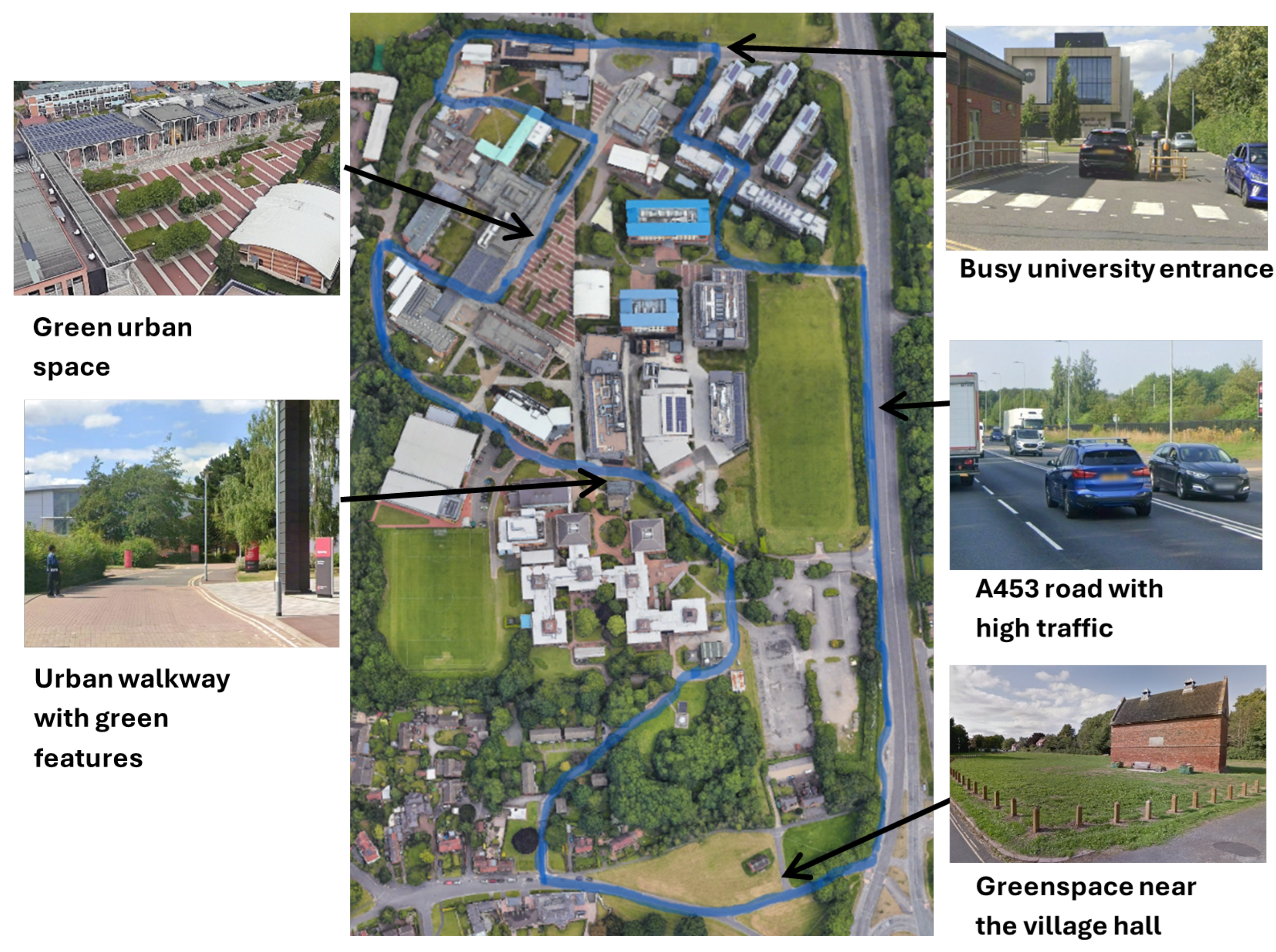
Figure 1. The predefined route labelled in blue highlight walked by the participants, with different features and environments highlighted.
Ijgi 15 00142 g001
Figure 2. PCA map plotting all the DigitalExposome dataset variables made up of Environmental, Physiological variables and Self-report label (wellbeing).
Ijgi 15 00142 g002
Figure 3. (a) PCA following removal of uncorrelated variables. (b) Further removal NH3 and NO2 to increase combined variance.
Ijgi 15 00142 g003
Figure 4. Heatmaps of PM2.5 concentrations with superimposed physiological and subjective wellbeing indicators. PM2.5 is shown alone in (A) and combined with IBI (B), HR (C), EDA (D), and wellbeing (E).
Ijgi 15 00142 g004
Figure 5. Heatmaps of PM2.5 concentrations showing only the extreme self-reported wellbeing values (1 = very negative (A), 5 = very positive (B)) overlaid. This targeted visualisation highlights where the lowest and highest wellbeing states occur relative to PM2.5 hotspots, supporting the identification of exposure-related wellbeing patterns.
Ijgi 15 00142 g005
Figure 6. Heatmap visualisations of six environmental pollutants: (A) NH3, (B) CO, (C) NO2, (D) PM1, (E) PM10 and (F) noise. Each map overlays the self-reported wellbeing label, scaled from white (high wellbeing) to purple (low wellbeing), to illustrate spatial correlations between pollutant concentration and perceived mental wellbeing.
Ijgi 15 00142 g006
Figure 7. A zoomed in perspective of the heatmap depicting noise overlayed on top of wellbeing. Two hotspots that indicate a break in the correlation are highlighted with red circles.
Ijgi 15 00142 g007
Figure 8. Ten participants’ PM2.5 data visualised as a Voronoi Display, overlayed on top the same map of Clifton Campus.
Ijgi 15 00142 g008
Figure 9. (A) Voronoi visualisation of one participant’s PM2.5 data with legend to the right. (B) Only displays the hotspots above 10 μg/m3.
Ijgi 15 00142 g009
Table 1. Data description for environmental and physiological variables.
VariablesMeanMedianMinQ1Q2Q3MaxSkew.Kurt.
BVP (µV)−1.500.00−1050.00−36.020.0034.711075.00−0.0211.02
EDA (µS)0.350.180.000.120.180.264.543.9215.84
HR (bpm)100.20100.600.7191.23100.64108.96174.000.131.66
HRV (s)0.460.550.000.210.550.621.34−0.52−0.54
NH3 (ppm)878.60686.0015.00509.00686.001064.003794.001.301.40
Noise (dB)97.4096.4047.2094.5096.37100.30140.30−1.7319.95
Nitrogen Dioxide (μg/m3)38.1038.002.0030.0038.0042.3088.000.080.21
PM 1.0 (μg/m3)4.363.000.000.003.007.0065.003.2118.60
PM 2.5 (μg/m3)5.800.000.003.003.009.0065.002.007.10
PM 10 (μg/m3)7.303.000.000.004.0012.0065.001.884.40
Carbon Monoxide (ppm)453.00509.0047.00341.00509.00548.001201.00−1.400.50
Disclaimer/Publisher’s Note: The statements, opinions and data contained in all publications are solely those of the individual author(s) and contributor(s) and not of MDPI and/or the editor(s). MDPI and/or the editor(s) disclaim responsibility for any injury to people or property resulting from any ideas, methods, instructions or products referred to in the content.