Article

Reducing Extreme Commuting by Built Environmental Factors: Insights from Spatial Heterogeneity and Nonlinear Effect

1
MOT Key Laboratory of Transport Industry of Big Data Application Technologies for Comprehensive Transport, School of Traffic and Transportation, Beijing Jiaotong University, Beijing 100044, China
2
School of System Science, Beijing Jiaotong University, Beijing 100044, China
3
School of Transportation and Logistics, Southwest Jiaotong University, Chengdu 611756, China
*
Author to whom correspondence should be addressed.
ISPRS Int. J. Geo-Inf. 2025, 14(12), 487; https://doi.org/10.3390/ijgi14120487 (registering DOI)
Submission received: 13 August 2025 / Revised: 23 November 2025 / Accepted: 3 December 2025 / Published: 9 December 2025
(This article belongs to the Special Issue Spatial Data Science and Knowledge Discovery)

Abstract

Nowadays, the number of people enduring extreme commuting is increasing, exacerbating traffic problems and harming individual well-being. To quantify the extreme commuting, we propose an extreme commuting severity (ECS) index that combines the number of extreme commuting trips with their specific distances, where a one-way trip with a commuting distance of at least 25 km is regarded as an extreme commuting trip. In Beijing, the ECS index shows substantial spatial variability, with maximum values exceeding 30,000 for origins and 50,000 for destinations, underscoring the severe commuting burden in specific areas. By integrating the geographically weighted random forest (GWRF) with Shapley additive explanations (SHAP), we model both nonlinear effects and spatial heterogeneity in how the built environment shapes extreme commuting. Compared with benchmark models, the proposed GWRF model achieves the highest predictive performance, yielding the largest R2 and the lowest absolute and relative indicators across both generation and attraction scenarios. Notably, the GWRF improves explanatory power over the global model by a substantial margin, highlighting the importance of incorporating spatial heterogeneity. SHAP-based global importance results show that residential density (17.58%) is the most influential factor for ECS, whereas in the attraction scenario, company density exhibits the strongest contribution (20.7%), reflecting the strong pull of major employment clusters. Local importance maps further reveal pronounced spatial differences in effect direction and magnitude. For instance, although housing prices have modest global importance, they display clear spatial heterogeneity: they exert the strongest influence on extreme commuting generation within the Fourth Ring Road and around the North Fifth Ring, whereas in the attraction scenario, their effects concentrate in the southern part of the core area. These findings provide new empirical insights into the mechanisms underlying extreme commuting and highlight the need for spatially differentiated planning strategies.

1. Introduction

Commuting activities are a crucial component of daily transportation in urban areas. Amid global urbanization and job–housing spatial allocation, increasing commuting durations and distances have become widespread across major cities and metropolitan regions worldwide. In Europe, approximately 5–10% of commuters take more than 60 min one way to work [1], while in Canada, the figure exceeds 9% [2]. As reported by the China Academy of Urban Planning and Design [3], 12% of urban residents in major cities commute for more than 60 min. Scholars have noticed this phenomenon and defined duration- or distance-unbearable commutes as extreme commuting [4,5]. The predominant viewpoint is that extreme commuting trips could exacerbate traffic congestion and air pollution [6]. Moreover, long commuting is believed to negatively affect personal well-being [7], causing fatigue, stress, and even mortality risk [8,9]. Therefore, understanding how extreme commuting occurs and how to mitigate its negative effects is critical for sustainable urban development.
Researchers widely agree that the built environment is closely related to the formation of commuting [10,11,12,13]. However, extreme commuting remains insufficiently understood. It typically involves longer distances or durations and shows distinct spatial patterns and drivers—often concentrating on urban outskirts and linked to housing-price and job-access imbalances [14]. These distinctions motivate studying the formation of extreme commuting separately from general commuting. A proper measurement of extreme commuting is the first step toward understanding this phenomenon. Many prior studies use either the extreme commuting rate (the proportion of extreme commutes in a given area) or a binary individual indicator (0 for non-extreme, 1 for extreme) as the dependent variable [14,15,16,17]. However, this binary approach—whether via an area rate or an individual indicator—overlooks variation in the severity of extreme commutes. For instance, under a 25 km distance criterion, a 30 km commute and a 100 km commute would both be labeled “extreme,” even though the latter imposes a much greater time and cost burden. Treating these cases as equivalent is problematic and underscores the need for a more nuanced index.
Another limitation concerns the modeling of extreme commuting. Mainstream global models typically assume linear, spatially uniform relationships, which obscures threshold effects and local variation [1,2]; the geographically weighted regression (GWR) model relaxes the spatial stationarity assumption but remains fundamentally linear [16]. Conversely, machine learning models capture nonlinearity yet are commonly estimated at a global scale, offering limited place-specific interpretability [11,18]. Recent integrated approaches that reconcile nonlinearity with spatial heterogeneity are still emerging but seldom target extreme commuting.
In light of these gaps, this study aims to advance the understanding of extreme commuting by integrating a severity-based measurement and a spatially explicit modeling approach. We focus on Beijing as a case study to examine how built-environment characteristics shape extreme commuting patterns and how these relationships vary across space.
This study makes three main contributions. First, it develops the ECS index that incorporates both the number and distance of extreme commuting trips, addressing limitations of binary or rate-based measures. Second, it introduces an explainable GWRF–SHAP framework capable of jointly modeling nonlinearities and spatial heterogeneity—an analytical capacity rarely applied in extreme commuting research. Third, using large-scale commuting data from Beijing, the study identifies and visualizes spatially varying impacts of built-environment factors on extreme commute patterns in Beijing, providing an empirical basis for targeted and differentiated planning strategies.
The remainder of this study is as follows: Section 2 presents a review of the relevant literature. Section 3 details the data and the case study area. Section 4 details the methods employed to analyze how built-environment factors relate to extreme commuting severity. Section 5 reports the model results and examines the nonlinear and spatial heterogeneity effects observed in Beijing. Section 6 presents a comparison with other works and discusses the implications for policy and planning in practice. Section 7 concludes the paper and lists potential biases.

2. Literature Review

2.1. Measurement of Extreme Commuting

The formal delineations of extreme commuting and its related terms, such as long super and heavy-burden commuting, are primarily examined in Western nations [1,14,19]. The measurement of extreme commuting primarily relies on commute duration and distance; however, there is no consensus on the threshold values adopted across urban transportation studies. Commuting duration is widely used to characterize individual commuting behavior, reflecting factors such as traffic conditions and travel mode. Various scholars used commuting duration to measure extreme commuting. Bai et al. adopted 90 min as a typical one-way threshold for extreme commuting studies in the central Puget Sound region, USA [16]. Furthermore, other studies adopted the standard based on the American Community Survey and Public transit smart card records from Beijing in 2010 [20]. In Sweden, Sandow et al. set a 45 min one-way duration as a threshold to study long commutes [9]. According to one recent study on extreme commuting across Canada, Allen et al. defined extreme commuters based on three criteria, namely, one-way commute durations above 60 min, 75 min, or 90 min [2]. Moreover, various studies have measured extreme commuting using distance thresholds to determine urban granularity. At the urban agglomeration level, Mitra and Saphores measured long-distance commuting as one-way trips taking longer than 50 miles in California [14]. In rural England, a 20 km distance is applied to study the features of extreme commuting [5]. In an urban area, Maoh and Tang defined extreme commuting as trips longer than 17 km in Windsor, Canada [20]. Compared with the duration threshold, commuting distance may be a suitable proxy due to its close relationship with the negative externality effect, especially for urban restructuring [21]. From the land use and urban planning perspectives, the commuting distance can be appropriate for commuting measurement.
The measurement of extreme commuting is commonly divided by aggregation level into two categories: micro-level metrics defined for individuals or households, and areal-level metrics defined for geographic units (e.g., traffic analysis zones, census tracts, or grids). Consequently, the dependent variables of extreme commuting in these two types of studies differ accordingly. At the individual level, the explained variable is commonly defined as a dichotomous variable, indicating whether a trip qualifies as extreme commuting [2,4,17,22,23]. Furthermore, a study on extreme commuting uses the household as the basic unit of analysis [14]. If at least one household member engages in extreme commuting, then the dependent variable is set to 1; otherwise, it is set to 0. Moreover, the duration or distance of extreme commuting can be examined to identify how various factors influence its occurrence [15,19,24]. At the geographical unit level, scholars prefer to use the extreme commuting rate as the dependent variable [25]. Bai et al. examined the relationship between extreme commuting rates and land use and socioeconomic factors across census tracts in central Puget Sound [16]. Tong et al. considered the share of high-burden commuters in each traffic analysis zone in Wuhan to explore the association between commuting burden and the built environment [23]. Unfortunately, the extreme commuting rate overlooks the number of extreme commuting trips and the internal variations across different distances within a spatial unit.

2.2. Factors Influencing Commuting Burden

Commuting is widely regarded as a multifaceted individual choice involving the trade-off of various costs and benefits. According to previous studies, commuting burden, including commuting distance and commuting duration, is mostly determined by two factors—demographic attributes and built environment.
Some variations in commutes can be attributed to different demographic attributes. Several researchers have found that female commuters tend to commute shorter distances than male family members, as they often bear more familial responsibilities, an idea supported by the household responsibility hypothesis [24,26,27]. The bulk of studies have analyzed the association between car ownership and commuting burden, and the results generally indicate that driving a private car can often lead to longer commutes [5,28,29,30]. Regarding the relationship with income and age, research conclusions largely vary [31,32,33]. In addition, education [34], race [35], and institutional constraints [36] can influence people’s commuting burdens.
On the contrary, many studies have explored how the built environment influences commuting burden [10,12]. Specifically, heavy-burden commuting is often associated with built-environment characteristics that leave individuals with limited alternatives [16,23]. Maoh and Tang found that built-environment factors, rather than demographic factors, were more strongly associated with heavy-burden commuting than with normal commuting [19]. Land use factors, job density, and transportation infrastructure factors significantly contribute to the heavy commuting burden [19,24,37]. Generally, mixed land use is associated with long commuting; however, Raman and Roy found that if the land use mix exceeds a suitable threshold, it may cause congestion [38]. In addition, job density and residential density are vital in determining commuting burden [39,40]. Taking Beijing as a case study, Zhao demonstrated that greater distance from the city center is linked to longer commuting times [41]. Bai et al. found that longer distance to the nearest growth center is positively related to the possibility of extreme commuting [16]. Moreover, the effects of traffic infrastructure on commuting burden remain inconclusive regarding whether they are related [40]. Interestingly, house prices may also contribute to increased commuting burdens, as high costs can push individuals to reside farther from their workplaces [13,25].

2.3. Methods of Quantifying the Relationship Between the Built Environment and Commuting Demand

In previous studies, various methods have illustrated built environment–commuting linkage. Traditionally, studies have used linear or generalized linear models, such as multiple linear regression [36] and the logistic model [2]. Given the linear assumptions, the influences of factors are constant, ignoring the effective range and threshold effect [10]. Notably, based on the geographically weighted regression model (GWR) [16], the spatial variations were proven in a previous study. Recently, researchers have used machine learning models to examine the nonlinear associations between the built environment and commuting trips, such as random forest [18], gradient boosting decision trees (GBDTs) [11], and the extreme gradient boosting trees model [42]. However, these nonlinear methods based on global-scale analysis were unable to show spatial heterogeneity, potentially ignoring the regional differences of each factor.
Fortunately, some scholars have begun investigating the association between the built environment and traffic system combined with spatial heterogeneity and nonlinear relationships. Wu et al. applied a tree-boosting algorithm integrating the Gaussian process and random effects model (GPBoost), considering the spatial instability effect [43]. Although the prediction accuracy has improved, this method remains a global model that cannot visualize results specific to different geographic units. Another study considered Wuhan as a case study, using a spatial weighted GBDT method to capture the nonlinear influence of built-environment factors on commuting burden [23]. This method combines spatial kernel functions in GWR with GBDT. However, since GBDT is a sequential tree structure, the initialization of spatially weighted results may be continuously influenced by the weighting of residuals in each iteration of the algorithm. Therefore, the validity of this model may require further verification. Moreover, the GWRF regression model [44], integrating GWR with random forest, was proposed and applied in studies on the relationship between built-environment factors and traffic trips, such as intercity commuting [13] and intermodal transit trips [45]. Building on advances in geographically weighted machine learning, the GWRF framework estimates location-specific random forest models to capture spatially nonstationary relationships [44]. This design retains the ability to model nonlinearities while allowing effects to vary across space. Meanwhile, because GWRF is a geographically weighted extension of random forests, it inherits RF’s relative robustness to correlated predictors via feature subsampling and decorrelated splits. This allows us to retain predictors in their objective empirical distributions without aggressive preprocessing.
To understand the mechanisms underlying these methods, the partial dependency plot is traditionally applied to quantify the partial effect [10,43]. However, the partial dependency plot often overlooks the interaction effects between variables because it assumes that the variables are independent, which may not be true in real-world scenarios. Thus, scholars used the SHAP interpreter because it can provide some practical references when establishing land use planning for each spatial unit [46,47].

3. Data Preparation and Variables

3.1. Data Source

The extreme commuting data used in this study are from sample datasets of processed commuting trips from a location service-based platform called Baidu Maps. Baidu Maps is a leading mapping service provider in China, processing over 120 billion location service requests per day and serving more than 1.2 billion active smart devices per month, covering administrative divisions at all levels across the country. According to data from Qianfan, a Chinese provider of digital solutions for financial scenarios, Baidu Maps had a market penetration rate of 71.3% in China’s mobile mapping application market in 2019, ranking first among its competitors. For privacy purposes, all the data exported externally are presented as grid data and not in the form of individual disaggregated data. The dataset comprises more than 8.94 million morning rush commuting trip records in Beijing from 1 January 2019 to 30 June 2019 (181 days). These commuter trips are aggregated into grid commuter O-D matrix information in the form of a 250 m grid, and grid-based information is provided on the number of commuters; average commuting distance; ratio of men to women; proportion of private cars; and distribution of commuter population’s education, income, and consumption levels. These demographic portrait data are provided by Baidu. It generates portrait data from the user’s survey form, living habits, and shared data by other companies.
Supplementary geospatial data, such as point of interest (POI) data, road network data, bus stops, metro stations, and building footprints, were obtained from Amap and Baidu Maps. In addition, this study incorporates housing-price data from Lianjia in 2019. Moreover, data on Beijing primary and secondary school science and technology education demonstration schools were obtained from the Beijing Municipal Education Commission.

3.2. Study Area Classification

The study covers the entire city of Beijing, which was divided into uniform 1.25 km × 1.25 km grids, as shown in Figure 1. This level of granularity is suitable for analyzing urban traffic structure and capturing spatial heterogeneity in traffic demand [48]. Three typical areas are illustrated including Beijing core area, Tongzhou area (the planned urban subcenter in Beijing), and Yizhuang area (the only national-level economic and technological development zone in Beijing). Based on the data conditions, we selected grids where both the built-environment factors and commuting trips were non-zero as the study areas for extreme commuting generation and extreme commuting attraction, yielding 7362 and 6333 grids, respectively.

3.3. Threshold Setting for Extreme Commuting

In China’s policy context, the National Development and Reform Commission proposed a one-hour commuting circle as a key constraint for urban development in 2019. Consistent with this time benchmark, the 2024 Commuting Monitoring Report of Major Chinese Cities by the China Academy of Urban Planning and Design identifies 25 km as the threshold for ultra-long commuting in major urban areas [2]. This choice also has face validity from observed speeds: according to the 2019 China Urban Transportation Report [49], the average speed during peak commuting hours in Beijing is approximately 25 km/h, implying that a one-hour commute corresponds to an average distance of about 25 km—further corroborating the 25 km cutoff. Thus, our analysis focuses on workers whose one-way commute distance is 25 km or more. Figure 2 presents the selected extreme commuting statistics. Extreme commuting of over 25 km accounts for approximately 13.9% of the total commuting share. As a robustness check, we re-estimate the analyses with a 15 km threshold, because under peak-hour congestion and multimodal transfers, a one-hour commute often translates to a shorter distance in the urban core (Appendix A), indicating that our conclusions are not sensitive to reasonable variations in the distance threshold.

3.4. The Explanatory Definitions and Descriptive Statistics

The explanatory variables are the built environment and several demographic variables (Table 1). The built-environment variables of each grid comprise three components: land use, transportation, and socioeconomic attributes. For land use attributes, geospatial feature information can be extracted from POI data [50]. Each POI record contains three attributes—facility name, facility type, and geographic coordinates—and is classified into one of fifteen categories: residential district, catering service, shopping service, company service, entertainment service, cultural service, medical care, government office, scenic attraction, automotive service, financial service, hotel service, sports facility, parking service, or daily-life service. Because commuting behavior is strongly linked to both residential and workplace locations, we first include two land use variables, residential land use density in each grid (RD) and company land use density in each grid (CD), with the latter serving as a proxy for the spatial concentration of employment opportunities. In addition, land use intensity (LUI) in grid i can be calculated by the total density of all POIs in grid i. Land use mix (LUM) is assessed using the entropy mixture of the proportions of all types of POIs. The land use mix variable of grid i can be calculated using Equation (1), where p η represents the proportion of POI type h   and m denotes the number of POI types within grid i:
L U M i = η = 1 m p η ln ( p η ) ln ( m )
The transportation attributes can significantly affect trip generation [18,51]. According to previous studies, we selected five transportation attribute factors, namely, bus stop count (BS) [43], road density (RLD) [10], subway station count (ST) [43], distance to the core center (DCC) [43], and distance to the nearest regional subcenter (DNS) [45]. For core centers and subcenters, we referred to Beijing city plans (2016–2035) and used the centroid position to calculate distances. Finally, all spatial data were standardized to grid units using zonal statistics and the spatial join tools in ArcGIS. Socioeconomic variables, including housing price (HP) and school district (SD), were chosen and calculated. Informed by the literature review in Section 2.2, which highlights how demographic attributes relate to commuting, we included the following control variables to assess their relation to extreme commuting severity: the ratio of young commuters (YCs), the ratio of male commuters (MCs), the car-ownership ratio (CO), the proportion of commuters holding a bachelor’s degree or above (HE), the average income score (IS), and the average consumption score (CS) in each grid. Income levels were originally divided into five brackets, which we scored from 1 (lowest) to 5 (highest). Consumption levels were similarly classified into three groups and scored from 1 (low) to 3 (high). Here, the demographic portrait data provided by Baidu Maps are originally aggregated at the 250 m grid level. To align all datasets with the 1.25 km × 1.25 km analytical units, we spatially aggregated the demographic attributes by weighting each 250 m grid according to its number of commuters. Age, gender, and car-ownership ratios were computed as commuter-weighted proportions, while income and consumption scores were converted from categorical brackets and averaged using the same weighting scheme. This ensured statistical consistency and comparability across spatial units.

4. Methods

Figure 3 presents the framework used in this study. It mainly includes three parts: (1) quantitative measurement for extreme commuting, (2) nonlinear association modeling with GWRF considering spatial heterogeneity, and (3) GWRF interpreting with the SHAP model.

4.1. Extreme Commuting Index

To better quantify the severity of extreme commuting, we use a composite index that jointly captures two dimensions within each grid: (1) the extent—how many extreme commuting trips occur and (2) the intensity—how far those trips are. Analyzing only the number of extreme trips treats two different distance trips as equally severe, while using only the average distance makes the measure prone to skew from a few very long trips. Following evidence of diminishing marginal effects in commuting [8], distance enters the index through a logarithmic transformation, which preserves monotonicity yet imposes decreasing marginal loss as distance increases. This design yields a socially meaningful severity measure that balances “how many” and “how far.” The extreme commuting severity E C S for grid i is computed as follows:
E C S i = 1 n log ( e c d i j ) n 1 0 n = 0
In the above equation, e c d ij denotes the distance of the j th extreme commuting trip in grid i, and n refers to the number of extreme commuting in grid i. Moreover, we developed two models corresponding to the generation and attraction scenario.

4.2. GWRF Model

The GWRF regression model, which integrates the core principles of the GWR model into the random forest model (RF), thereby creating an effective local model that characterizes spatial heterogeneity [13,45,52], is applied separately to the extreme commuting generation and extreme commuting attraction scenarios in this study. The use of GWRF is motivated by two core characteristics of extreme commuting identified in Section 1, Section 2 and Section 3: (1) its spatially heterogeneous associations with the built environment and (2) its nonlinear and potentially threshold-based responses to the built-environment attributes. Traditional global or linear models cannot accommodate these mechanisms simultaneously. GWRF, by constructing localized random forest models calibrated with adaptive spatial weights, operationalizes our empirical strategy by allowing each grid cell to have its own nonlinear functional form. This design ensures that the model structure directly reflects the theoretical understanding of uneven urban development, spatial mismatch, and heterogeneous travel behavior across the metropolitan area.
For each scenario, the model is estimated at the spatial resolution of the 1.25 km × 1.25 km grids defined in Section 3.3. The study area for each model consists of all selected grids in which both built-environment attributes and commuting records are non-zero, ensuring that each observation meaningfully contributes to the analysis. The GWRF model involves several steps. First, the spatial weight matrix for each grid of W i = W ( w i 1 , w i 2 , , w i j , , w i n ) is constructed according to the distance decay rule, among which w i j is the spatial weight between grid i and grid j. Based on this, the overall spatial weight matrix for the extreme commuting study area comprising n grids can then be expressed as follows:
W = W 1 W 2 W i W n = w 11 w 12 w 1 n w 21 w 22 w 2 n w i 1 w i 2 w i n w n 1 w n 2 w n n
where W i refers to the spatial weight in grid i, and w i j reflects the utility of association between grid i and grid j decaying with distance. In this study, we adopted the bi-square weighting kernel function to represent this geographic delay utility. Thus, the weight between two grids is as follows:
w i j = 1 ( d i j / b w ) 2 2 d i j b w 0 d i j > b w
where d i j is the distance between grid i and grid j. b w is a bandwidth size. Like other geographically weighted regression methods, the selection of b w is critical for the GWRF model. A large b w may cause biased estimates, while a small b w may weaken robustness due to limited local samples. We adopt an adaptive kernel to calculate the spatial weighting [13], in which the bandwidth represents the number of nearest neighbors to be included in each local model, so that each local model uses a comparable number of nearest neighbors, which mitigates edge effects and density-driven variance imbalances in our unevenly distributed study grids. After this process, we built the spatial weight matrix based on the idea of the traditional GWR model, which can exert the geographical weight W i on nearby observations modeled in the local random forest at the regression grid i. Then, for grid i, the neighbors of each grid ( w i j 0 ) are determined via the spatial weight matrix and used as input to a local random forest. During the bootstrap sampling for each decision tree, grids assigned higher weights are more likely to be selected. Many unrelated decision trees are aggregated to form a local model in grid i. The regression equation in the local model calibrated in grid i can be formulated as follows:
Y i = f ( u i , v i ) ( x ) + ε i
where f ( u i , v i ) ( x ) is the local geographically weighted random forest model prediction for grid i, and ( u i , v i ) denotes the spatial coordinates of grid i’s center centroid. By repeating the above modeling procedure for every grid, we obtain a complete set of local GWRF models, enabling the relationship between ECS and the built environment to be analyzed at each individual grid.
The power of the GWRF model lies in its ability to allocate geographic weights to the observations used within each localized random forest. In addition, grid search combined with K-fold cross-validation is used to identify optimal GWRF parameters, reducing overfitting risk and mitigating the effects of data imbalance.

4.3. SHAP Model

To inform practical policymaking, understanding the impacts of different built-environment factors and their collective influence is crucial. The SHAP model employs the Shapley value, derived from game theory, to quantify and interpret the influence of independent variables on a dependent variable. To connect the local nonlinear GWRF results with practical interpretation, we adopt the SHAP model as an explainable machine learning tool. In the context of this study, SHAP provides a consistent way to decompose the predicted extreme commuting severity (ECS) into additive contributions from each built-environment attribute; this enables us to understand not only which variables are important, but how and in what direction they influence extreme commuting in different parts of Beijing.
The contribution of feature k for the GWRF prediction is quantified by its Shapley value, calculated as follows:
φ k = S Q k | S | ! ( q | S | 1 ) ! q ! f ( S { k } ) f ( S )
where φ k refers to the contribution of feature k, representing the marginal change in ECS that can be attributed to that feature; Q denotes the full set of built-environment and demographic factor variables, S denotes the subset of the input features, f ( S { k } ) represents the GWRF model results when the k feature and other features in S are included, and f ( S ) is GWRF prediction using features in S (without the feature k). The interpretable model is created using an additive feature imputation approach, and its linear form is defined as follows:
g ( z ) = φ 0 + k = 1 M φ k z
where z { 0 , 1 } M , with z = 1 indicating that the feature is observed and z = 0 when it is unobserved. Here, M denotes the number of explanatory variables, φ 0 represents the base ESC level, and φ k refers to feature k’s Shapley value.

5. Results

5.1. Distribution of E C S Index

Given Equation (1), we calculated the E C S index of each grid on both the generation and attraction scenarios, and the statistics and spatial distribution are presented in Table 2 and Figure 4. Areas with the highest E C S are in outer new towns and surrounding regions, while destinations are concentrated in the urban core, reflecting a flow from peripheral areas to the city center. The mean E C S at destinations exceeds that at origins, with a notably higher maximum, indicating that employment locations for extreme commuters are more spatially concentrated compared to their residential locations.

5.2. Model Performance

We conducted a spatial autocorrelation analysis on the extreme commuting severity using the global Moran’s I index (Table 3). The generation and attraction of E C S exhibited positive Moran’s I indices, with a highly significant p value of 0.000 (p < 0.01) and z scores > 2.58. These results confirm that E C S is not randomly distributed but rather exhibits spatial autocorrelation. Consequently, analyzing the spatial heterogeneity of this issue is essential.
We adopt the 3-fold cross-validation and grid search method to obtain the optimal parameters. When b w is 289 (296), the number of trees is 198 (223), and the number of features randomly selected for each split is 8 (8) in the generation (destination) scenario. Due to the substantial differences in the value ranges and measurement units of the independent variables, we standardized these variables to ensure a more balanced contribution from each feature during model training. In order to preserve the interpretability of the original mechanism underlying extreme commuting, no transformation was applied to the dependent variable.
To examine the performance of the GWRF model, we compared this model with the ordinary least squares regression model (OLS), RF, and GWR model. Three goodness-of-fit measures, namely, R square, root-mean-square error, and mean absolute error, are calculated in extreme commuting generation and attraction scenarios, as shown in Table 4. Because the ECS index has an inherently wide range, the absolute values of MAE and RMSE are numerically large but remain reasonable in scale. To provide a scale-free assessment, we additionally report two relative error metrics—the coefficient of variation of RMSE (CVRMSE) and the normalized MAE (NMAE). These indicators normalize the absolute errors by the mean level of the dependent variable and thus offer a clearer picture of model performance across different ECS magnitudes. As reported in Table 4, both RF and GWR outperform the global OLS model, while the proposed GWRF model consistently achieves the lowest errors—including the lowest CVRMSE and NMAE—in both scenarios, highlighting its superior ability to capture nonlinearity and spatial heterogeneity in extreme commuting in relation to the built environment.
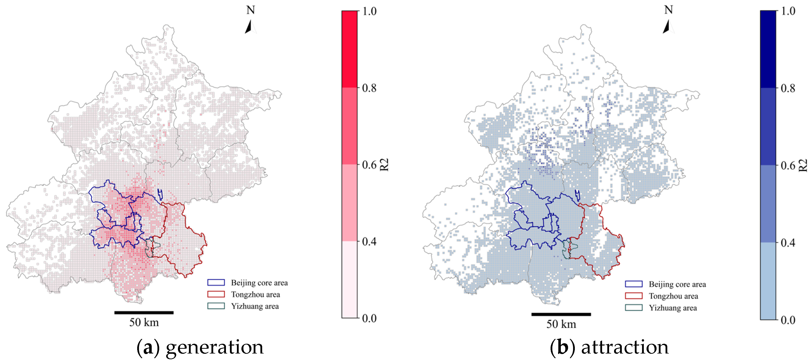
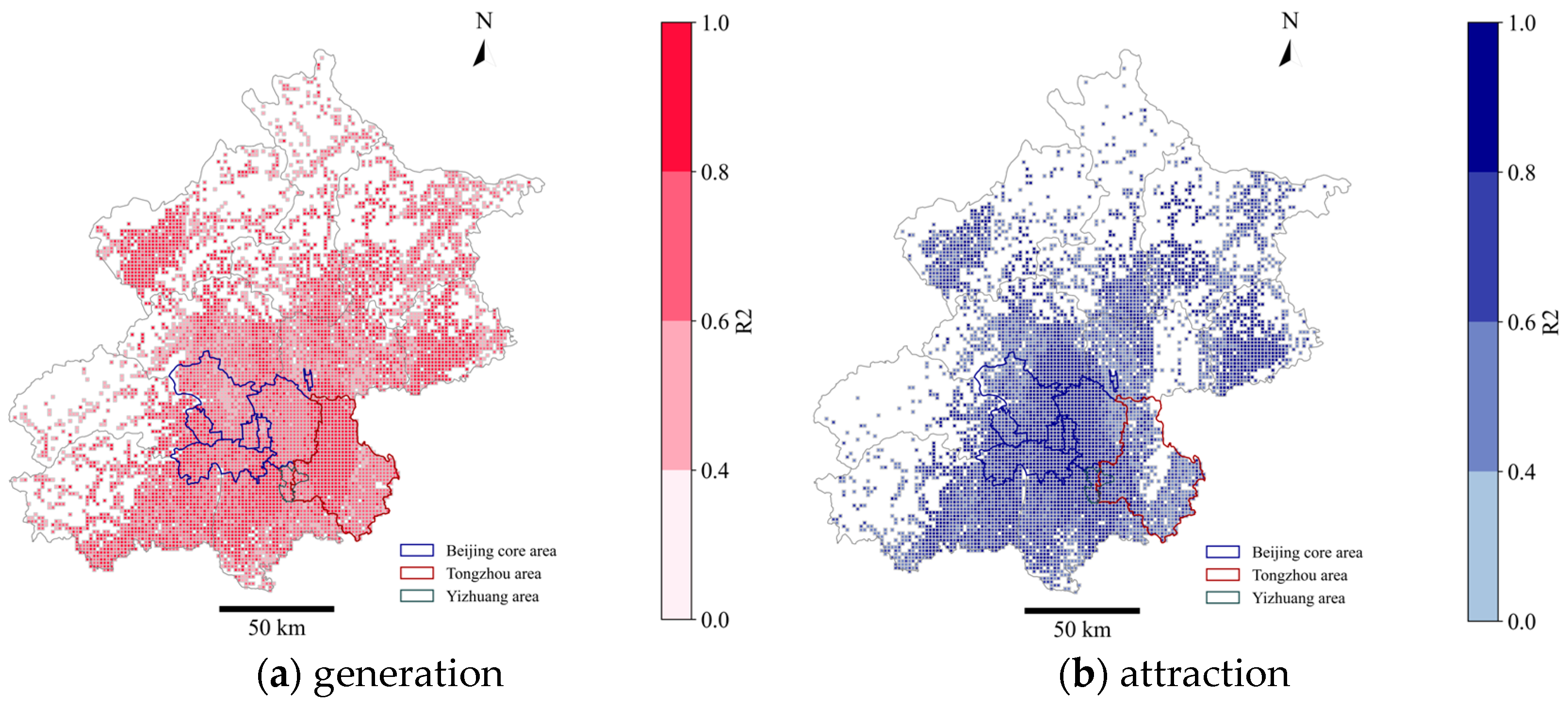
Figure 5 presents the local R2 distribution of GWRF under extreme commuting generation and attraction scenarios. On the generation side, the local values of extreme commuting severity R2 are relatively high in the outer new towns and the surrounding areas, such as satellite towns and more distant districts. These districts encompass the partial regions of Tongzhou, Fangshan, Shunyi, Pinggu, and Yanqing. Overall, the R2 distribution exhibits a characteristic of being high on the outside and low on the inside. Conversely, this differs on the attraction side. As shown in Figure 5b, the highest R2 values are concentrated in the center area in Beijing.

5.3. Spatial Distribution of Relative Importance

5.3.1. Overall Analysis

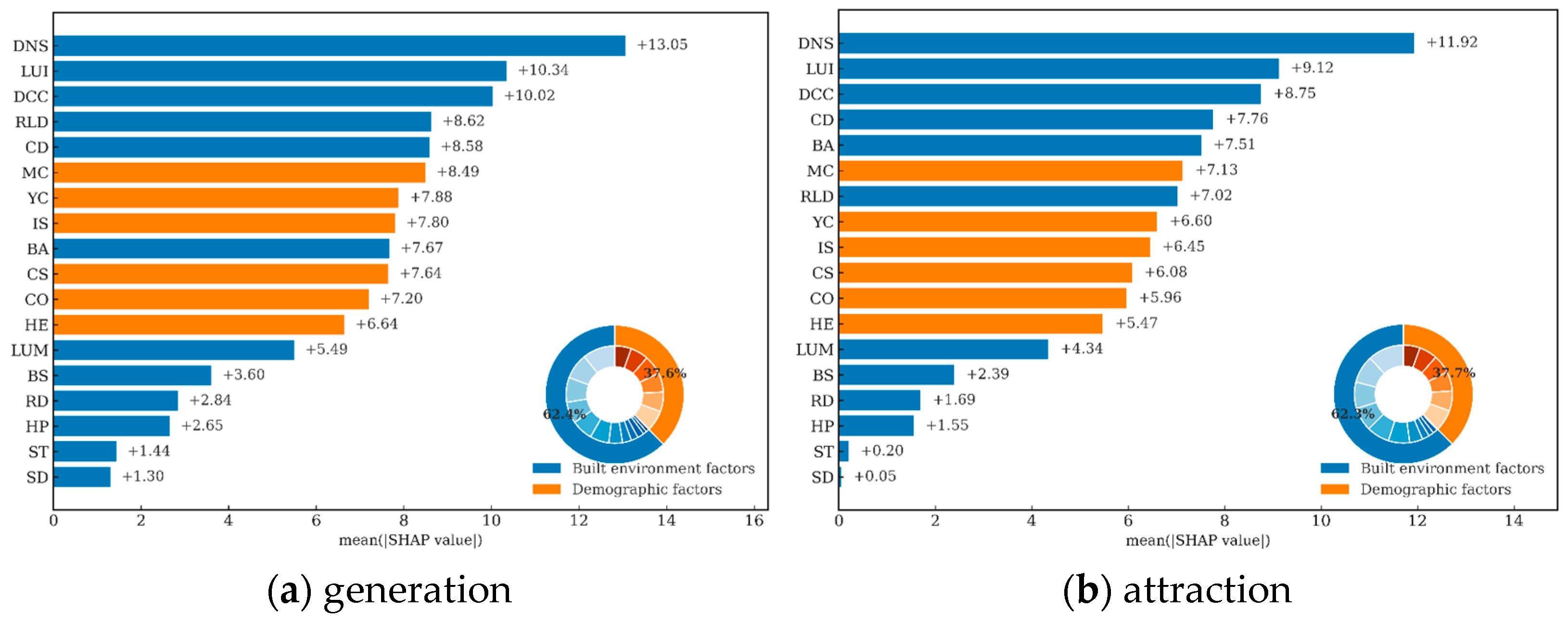
In this section, we analyze the spatial heterogeneity in the relative contributions of each factor using SHAP values. When estimating the relative importance, we calculate the average of the absolute SHAP for each local model. The average absolute SHAP ratio of the sum of average measures the global relative importance of variables, as shown in Figure 6. The global relative importance indicates the contribution of each variable. Specifically, as shown in Figure 5a, RD shows the strongest association with extreme commuting in the generation scenario, with an average relative importance of 17.58%, followed by LUI at 16.05%, whereas SD exhibits the weakest association. In the attraction scenario, a different pattern is observed. As illustrated in Figure 6b, CD is most strongly related to extreme commuting attraction. In addition, the nested-donut inset at the lower right of Figure 6a,b provides an intuitive summary of global importance. On the generation side, built-environment variables account for roughly 75% of the total importance; on the attraction side, their share exceeds 80%. This indicates that, relative to demographic attributes, the built environment plays a dominant role in explaining spatial variation in extreme commuting.

5.3.2. Generation Scenario

The local interpretation map (Figure 7) visualizes the influence and importance of the variable in each local grid on generation extreme commuting. Obviously, the importance of these variables varies through space. As shown in Figure 7a, RD plays a major role in the southern areas of Beijing, such as Fengtai, Fangshan, Daxing, and Tongzhou. A possible explanation is that in these areas, individuals can own a home at a low cost, resulting in a significant number of individuals with limited savings living in these areas that are far from their workplaces. Meanwhile, LUI is significantly important in Changping and Shunyi; hence, these places cannot disregard intensive and efficient development. RLD is substantially effective in a small area of Shunyi and southern Daxing. Another traffic infrastructure factor (i.e., BS) has a more evident impact in the south of Daxing District. The establishment of bus stops in this district can offer better transportation options for commuters. HP shows a significant association with the generation of extreme commuting in two key areas, namely, within the Fourth Ring Road and around the North Fifth Ring in Beijing. These regions have relatively high housing prices, suggesting that price fluctuations greatly affect E C S in these areas. LUM is relatively related to the extreme commuting negation in the southeast of Beijing, where the potential influence of land use allocation should not be disregarded.

5.3.3. Attraction Scenario

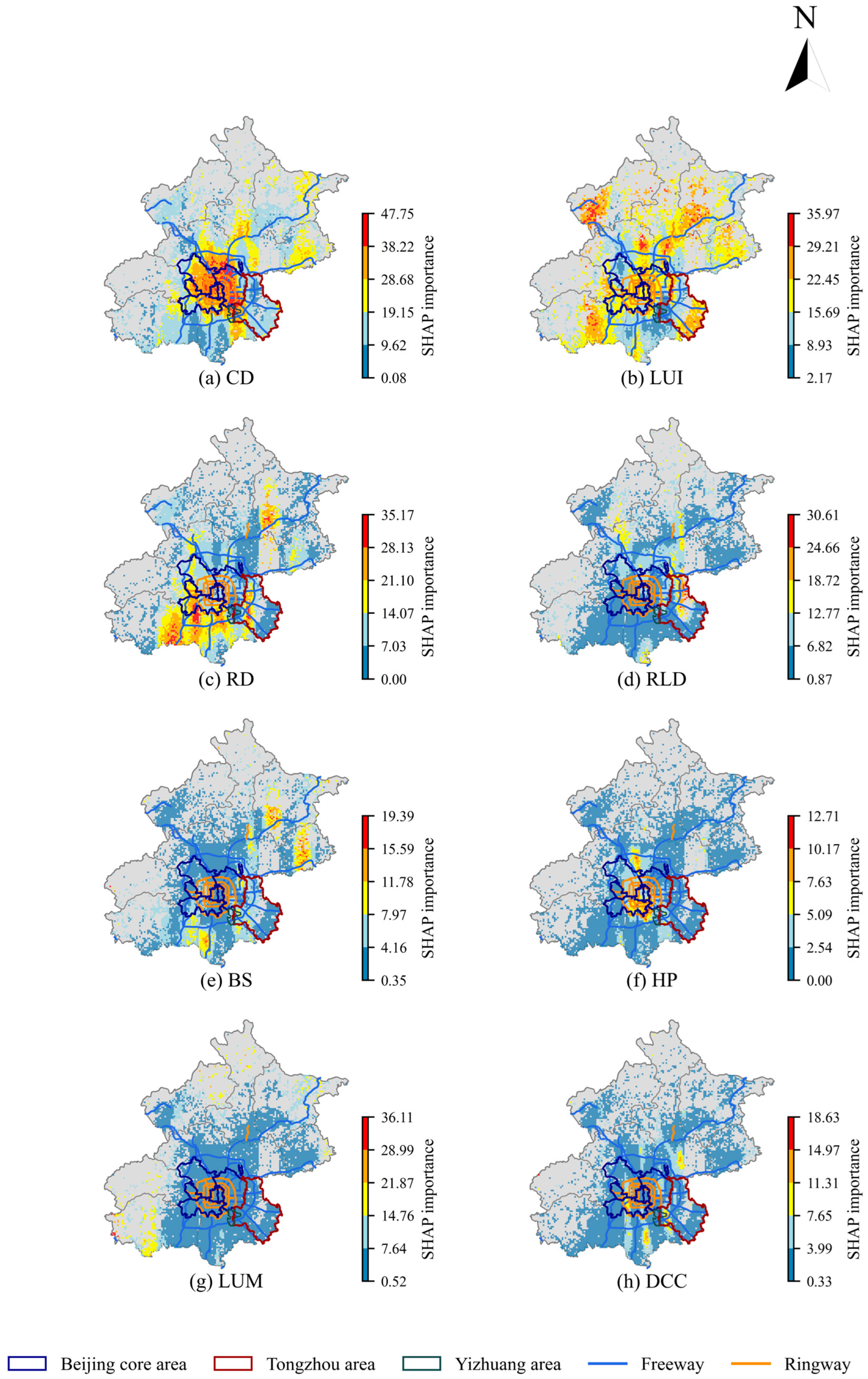
Figure 8 presents the spatial distribution of the importance of eight typical built-environment explanatory variables in the attraction scenario. Clearly, there is a strong spatial interaction between these built-environment variables and extreme commuting severity. Figure 8a,b present the spatial distribution of CD and LUI. Compared with the core area within the Fifth Ring Road, the associations of CD and LUI with extreme commuting severity are weak in the suburban regions around ring areas. This can be attributed to the strong industrial agglomeration effect within the core area, where a large concentration of high-quality job opportunities attracts suburban residents, thereby exacerbating extreme commuting. By contrast, as shown in Figure 8c, RD exhibits an opposite trend, showing a weaker association in the core area but a stronger association in regions such as Fangshan, Daxing, and the emerging urban subcenter in Tongzhou.
With respect to traffic infrastructure, the associations of RLD and BS with the severity of extreme commuting destinations exhibit significant spatial heterogeneity. Although some areas are almost unaffected, in certain localized regions, their importance can exceed 15%. Figure 8d illustrates that the areas that have the strongest recent association with extreme commuting severity are concentrated in Tongzhou. Moreover, Figure 8e indicates that the influence of BS is more prominent in the suburban and outer suburban regions of Daxing, Pinggu, and Miyun. The overall importance of LUM and HP is relatively low. Furthermore, compared with other variables, their spatial distribution does not significantly vary (Figure 8f,g). The importance of HP shows the strongest association concentrated in the southern areas within the Fifth Ring Road. This can be attributed to the overall lower housing prices in Fengtai and Daxing District (Yizhuang area), where people are more sensitive to price changes. However, the overall association of HP with extreme commuting severity remains weak, possibly because a substantial portion of the population does not own a home and rental prices are not considered in this study. Furthermore, as shown in Figure 8h, areas most sensitive to distance from the city center are concentrated in Shunyi, Shijingshan, Daxing, and Yizhuang, all of which have affluent residential communities. Therefore, the relationship between these factors warrants further investigation in other studies.

5.4. Nonlinear Associations Among Different Regions

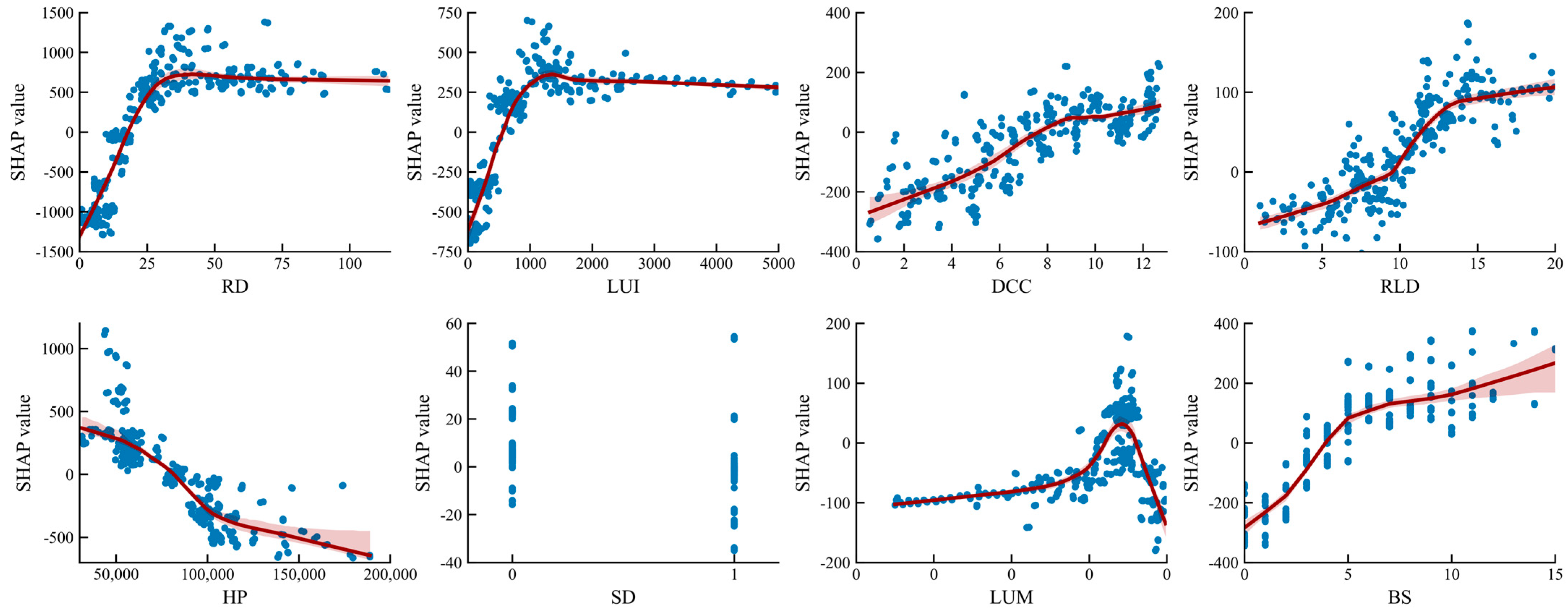
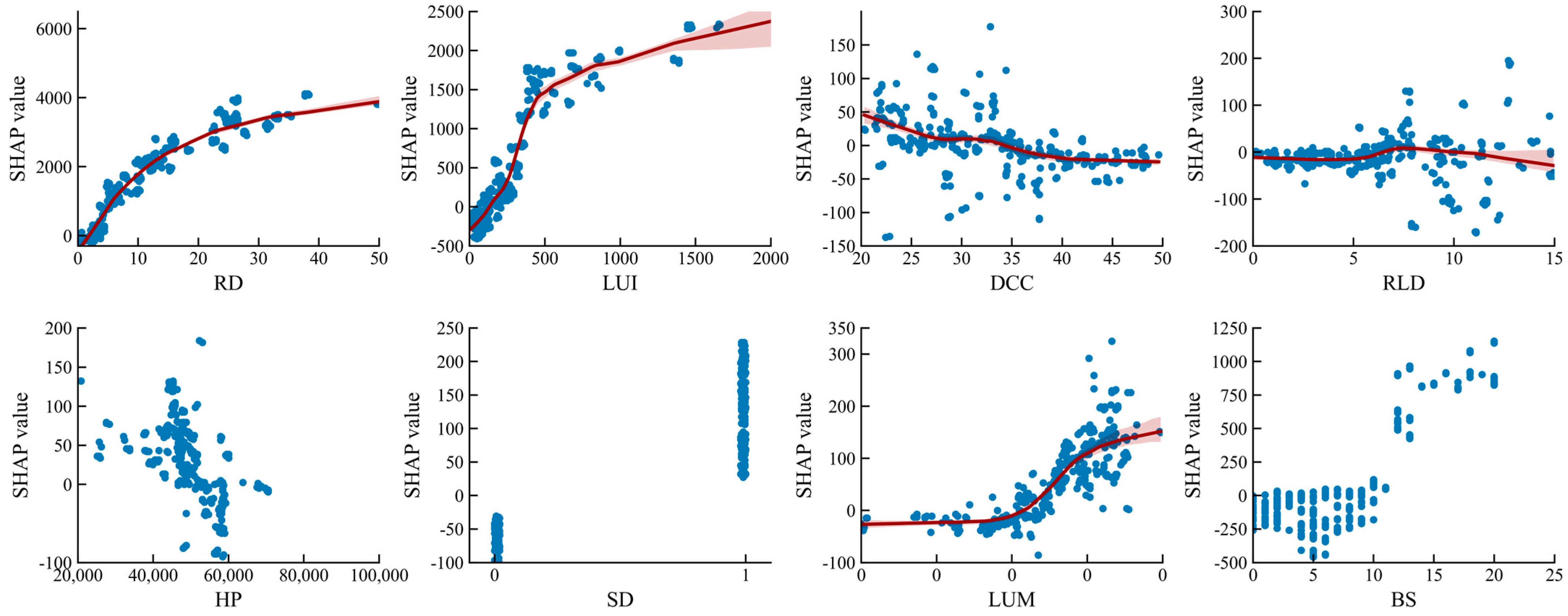
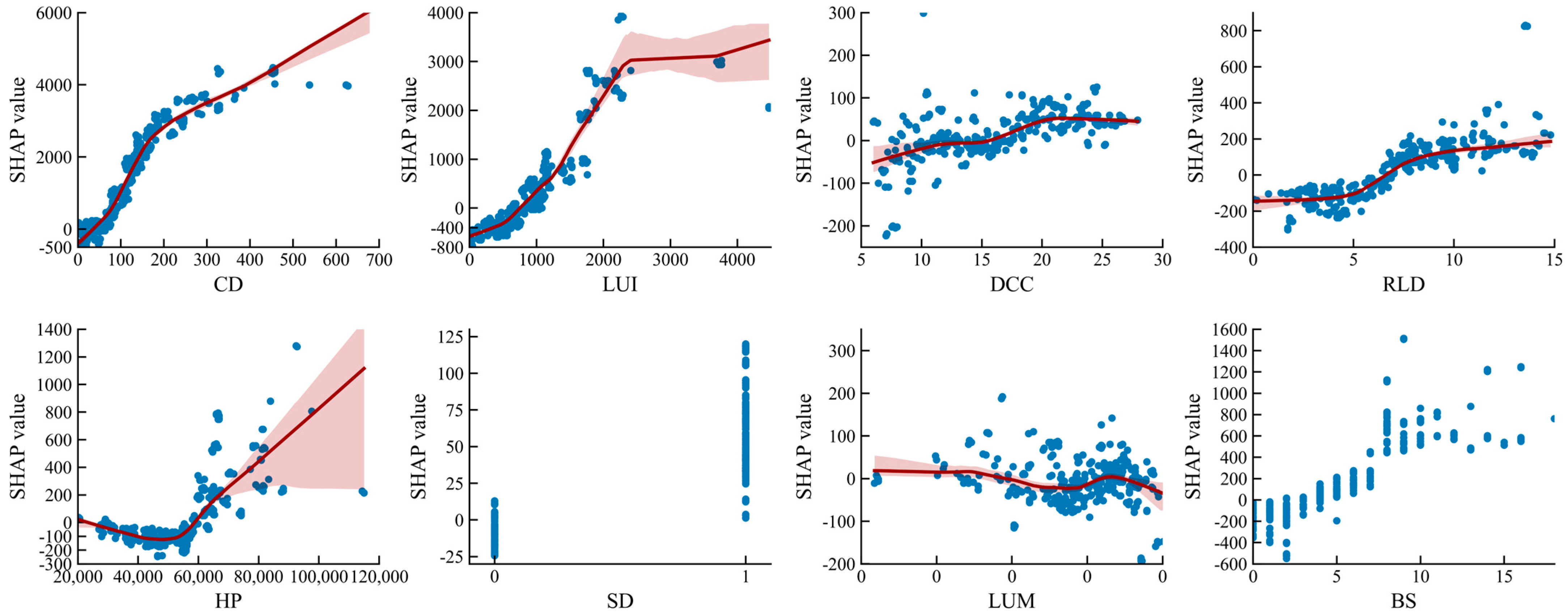
To further investigate the detailed nonlinear relationship between built-environment factors with extreme commuting and whether differences exist across regions, three typical areas, the locations of which are shown in Figure 1, are selected for analysis. We present SHAP scatterplots to depict the relationships between selected built-environment variables and E C S , accompanied by red trend lines to highlight general trends.
As shown in Figure 9, Figure 10 and Figure 11, the comparative analysis of extreme commuting generation between different regions reveals interesting patterns. Almost all built-environment factors exhibit nonlinear associations with the generation of extreme commuting in all three districts. RD and LUI correlate with E C S , with a negative to positive effect change in three models. However, the fluctuation in relationships differs. In the core area, the nonlinear relationship shows an initial increase, stabilizing after a threshold is reached, whereas in Tongzhou and Yizhuang, the threshold is less pronounced. The direction, threshold, and effect intensity of some variables vary across regions. For example, the association of RLD with extreme commuting severity is minimal in Tongzhou, with a SHAP value nearing zero, whereas in the core area, a positive correlation is observed. The association of DCC shows a quasilinear upward trend in the core area, a U-shaped trend in Yizhuang, and a quasilinear downward trend in Tongzhou. This variable appears to have a positive correlation in the core area. But this relationship changed in Tongzhou. In this area, E C S initially decreases as DCC increases, suggesting that the negative association weakens. HP only reveals a clear pattern in the core area, where E C S significantly decreases as HP increases, which is consistent with the previous literature [23]. Compared with the effects on the core area, E C S is higher in areas with SD than in nonschool district areas. In Tongzhou and Yizhuang, this finding confirms that residents are more inclined to live near school districts for their children’s education, even if it means bearing high commuting costs. The impact of LUM varies across the three regions, with distinct trends and directions. In the core area, it follows an inverted U-shape, with a clear turning point at a threshold of 0.7. Beyond this value, LUM typically exhibits a negative correlation with E C S . Meanwhile, in Yizhuang and Tongzhou, LUM exhibits a strong positive correlation with ECS once it exceeds a threshold of 0.5, and the curves begin to flatten after reaching thresholds of 0.65 and 0.6, respectively. This finding suggests that in the Beijing core area, the highly mixed use of land may alleviate extreme commuting in the traffic demand generation scenario.
From the extreme commuting attraction perspective, Figure 12, Figure 13 and Figure 14 present the nonlinear associations between built-environment variables and E C S among three typical regions. The impact of CD on attraction of extreme commuting exhibits a quasilinear growth trend in the core area and Tongzhou. At the low levels of company density, the relationship with E C S is negative, with the SHAP value smaller than 0. However, as the surrounding company density increases and crosses a certain threshold, E C S gradually worsens. This threshold is approximately 300 in the core area and 50 in Tongzhou. Notably, in Yizhuang, CD shows a pronounced nonlinear association with E C S . When CD is between 60 and 200, E C S rapidly increases; however, beyond this range, the rate of increase significantly slows down. Therefore, while it is beneficial to attract businesses in low-density areas, excessive clustering of businesses in high-density areas should be avoided. In addition, it is essential to adapt to local conditions because the optimal CD varies depending on the development characteristics of each region. The association of LUI follows a similar quasilinear growth pattern to that of CD. As for LUM, the nonlinear association exhibits distinct patterns across the core area, Yizhuang, and Tongzhou. In the core area, LUM has a clear threshold effect on the attraction of extreme commuting. When the LUM exceeds 0.7, it significantly suppresses E C S . Therefore, establishing highly mixed-use community structures is recommended in the core area. By contrast, Tongzhou exhibits the opposite trend. When the LUM exceeds 0.6, the SHAP value increases. This may be attributed to a mismatch between the highly mixed commercial zones and residential facilities in Tongzhou because the area has a high rate of cross-district residence among its working population. Moreover, we found that RLD and BS promote E C S at the destination once a certain threshold is reached in all three areas. A possible explanation is that a more developed transportation infrastructure increases local accessibility, thereby expanding the range over which residents can seek employment, making extreme commuting more prevalent. An interesting phenomenon of the SD in Tongzhou and Yizhuang is that locations within school districts generally make a positive contribution to SHAP values, whereas locations outside school districts negatively contribute. This suggests that areas with school districts have a strong attraction for extreme commuting. However, this effect is not as apparent in the core area. The effects of HP on extreme commuting are more pronounced in Yizhuang, showing a clear range of influence and threshold effects. When housing prices exceed CNY 57,000 per square meter, extreme commuting severity significantly increases. This may suggest the maximum HP level that commuters working in Yizhuang are willing to tolerate.

6. Discussion

6.1. Comparison with Related Studies

Compared with previous studies on extreme commuting, our research uses more reliable big data, introduces an improved index E C S that captures extreme commuting more accurately, and employs hybrid interpretable machine learning models, effectively addressing spatial heterogeneity and nonlinear relationships.
Compared with traditional survey data, big data sources can provide larger samples with broader coverage for extreme commuting research [15,17]. Some scholars argue that big data often lack detailed demographic attribute information. Fortunately, our research benefits from access to aggregated demographic attribute data at the grid-cell level. These data were collected by Baidu Inc. in accordance with informed user consent and compliant privacy protection policies and were aggregated at the grid-cell scale to ensure privacy. Consequently, our study not only reduces sampling bias inherent to traditional survey methods but also incorporates the impacts associated with demographic attributes.
Previous studies primarily employed extreme commuting rate as the study object, neglecting both the total number of extreme commuters within TAZs and the internal variations among different extreme commuting trips [16,26]. When using extreme commuting rate as the dependent variable, the importance ranking of explanatory variables shifts significantly (shown in the supplementary analysis in Appendix B, Figure A3), diminishing the roles of residential density at the origin and employment density at the destination. In reality, excessively dense residential development or overly concentrated employment areas may generate substantial extreme commuting trips due to residential-employment mismatches. Furthermore, by comparing the local R2 values, we observed that models using extreme commuting rate as the dependent variable generally yield local R2 values below 0.6, with most areas in the generation model even falling below 0.4 (Figure A4). In contrast, the ESC-based models proposed in this study exhibit significantly higher explanatory power. This finding, to some extent, supports the notion that the new nonlinear index for measuring extreme commuting severity (ESC) proposed in this study serves as a more scientifically robust indicator for capturing regional extreme commuting.
In this study, we used a hybrid interpretable machine learning model considering the spatial weights. This model can effectively capture the spatial heterogeneity of variable importance, highlighting that the association of the same factors varies across regions. It can therefore be used to identify which variables require greater attention in specific areas. The GWRF model demonstrated superior explanatory performance (highest R2) in both commuting generation and attraction scenarios compared to the OLS, RF, and GWR models. Recently, there has been an increasing interest in exploring the nonlinear relationships between the built environment and travel behaviors [10,45,47,52]. Collectively, these studies indicate that linear assumptions could introduce bias and lead to misleading interpretations. Interpretable machine learning models can offer advantages for better understanding the complex relationships between built environments and commuting behaviors. Applying such models to study extreme commuting allows consideration of both nonlinear effects and spatial heterogeneity, warranting further empirical exploration in future research.

6.2. Policy Implication on Reducing Extreme Commuting

Through analyzing the distribution of built-environment importance in local models and partial dependence plots, we found that nearly all built-environment attributes exhibit nonlinear relationships with E C S , both in the commuting generation and attraction scenarios. Moreover, these relationships display spatially heterogeneous characteristics across different regions. These findings offer valuable insights and urban planning recommendations aimed at alleviating commuting burdens.
(1)
Regional differentiation suggestions based on important variables
In the extreme commuting generation scenario, RD plays a major role in the southern areas of Beijing, where economic development lags behind and high-quality employment opportunities are limited. Residents in these districts are more likely to experience extreme commuting due to the spatial mismatch between housing and jobs. Simply increasing road infrastructure in these areas is unlikely to alleviate commuting burdens and may even induce longer-distance travel. Instead, policies should focus on fostering local employment through the development of decentralized business hubs and innovation parks to promote a better job–housing balance within southern districts. LUI shows the higher relevance in suburban areas beyond the Fifth Ring Road, likely due to the saturation of land development in the urban core. In these regions, strategic densification can promote more compact land forms that support shorter commutes.
From the perspective of commuting attraction, SHAP-based partial dependence plots reveal that excessively high concentrations of companies in the core area can significantly exacerbate extreme commuting pressures. Therefore, promoting moderate-scale business clusters, rather than unchecked centralization, is more effective in mitigating commuting overload. Policymakers could support the relocation of selected large enterprises and the redistribution of non-capital functions to suburban centers or surrounding cities, in line with Beijing’s regional integration strategies. This decentralization can alleviate spatial imbalance and distribute employment opportunities more evenly across the metropolitan region. Of course, it is important to acknowledge that promoting decentralization in Beijing faces substantial practical constraints. Large enterprises and headquarters rely heavily on central locations due to strong agglomeration economies, dense business networks, and access to high-skilled labor. Relocation also involves high sunk costs, institutional inertia, and potential efficiency loss. Meanwhile, the attractiveness of many suburban areas remains limited by insufficient public services, amenities, and transit connectivity, which weakens their capacity to accommodate high-quality employment functions. Despite these barriers, Beijing’s ongoing “non-capital function dispersal” provides a feasible pathway, as it enables relocation through strong governmental coordination and long-term institutional arrangements. Under such a framework, decentralization should not be pursued as simple physical relocation, but as part of a broader urban restructuring strategy: enhancing the attractiveness of suburban centers and improving transit accessibility. Only when suburban areas offer competitive amenities and accessibility advantages can decentralization genuinely reduce extreme commuting burdens.
In addition, short-to-medium-term relief may be achieved through improvements in mobility services. Flexible, demand-responsive transit options—such as customized buses, on-demand shuttles—can enhance accessibility for residents in remote or poorly connected areas and help alleviate pressure on existing transport networks.
(2)
Targeted local strategies considering nonlinear associations and thresholds
As for the extreme commuting generation scenario, higher HPs correlate with lower E C S in the core area—a seemingly counterintuitive pattern. This may reflect the greater residential flexibility of high-income individuals, who can afford to live closer to employment centers and thus minimize commute times. From the commuting attraction perspective, HP shows the highest association in southern areas within the Fifth Ring Road, where higher HPs correspond to more extreme commuting, likely because individuals employed in these areas prioritize job availability over commuting convenience and are sensitive to housing costs and are pushed to live in more affordable, distant locations. These findings suggest the need to expand affordable and public rental housing near central and southern employment hubs to improve job–housing balance, reduce commuting burdens for low-and middle-income workers, and promote social equity. While desirable, expanding affordable or public rental housing in these locations faces substantial constraints in Beijing, where high land prices and limited developable land make large-scale new supply challenging. Practical implementation is therefore more likely to rely on diversified mechanisms—such as acquiring or leasing existing stock housing—rather than extensive new construction. These complexities indicate that housing-based interventions should be viewed as long-term structural strategies. Moreover, they highlight the equity dimension of extreme commuting—a topic that warrants further research.
The results of LUM show spatially variable, threshold-dependent impacts. In the core area, extreme commuting only decreases significantly when LUM surpasses a certain threshold, while in Yizhuang and Tongzhou, the effects of LUM are reversed beyond specific thresholds. These patterns suggest that an overly aggressive implementation of mixed-use development in some peripheral districts may create unintended consequences—such as land use fragmentation, functional mismatches, or inefficient job–housing distributions. Therefore, land use planning must be context-sensitive: while dense, mixed-use development is suitable and effective in the core area, more balanced and functionally coherent planning is needed in rapidly urbanizing suburban areas. In districts like Yizhuang and Tongzhou, this could include focusing on consolidating employment clusters, improving local job–housing balance, and avoiding excessive land use mixing that undermines spatial coherence.

7. Conclusions

In this study, we used multisource data to examine the associations between built-environment factors and the generation and attraction of extreme commuting in Beijing. A new nonlinear index was proposed to measure extreme commuting severity, considering the number and the internal variations of extreme commuting trips. Compared with previous studies, we introduced a hybrid interpretable machine learning framework—GWRF-SHAP—that effectively captures spatial heterogeneity and nonlinear effects, offering insights into the underlying mechanisms of each factor. This approach holds practical value for policymakers and urban planners and warrants broader empirical application.
First, residents are currently experiencing a heavy commuting burden, with approximately 13.9% of the commuters’ one-way trips exceeding 25 km. The spatial pattern reveals that extreme commuting indicates a predominant commuting flow from the periphery to the city center.
Second, RD and CD are key drivers of extreme commuting in both generation and attraction scenarios. RD has the strongest association in the generation scenario, contributing 17.21% to the model’s explanatory power, while CD is the dominant factor in the attraction scenario, with RD ranking third.
Third, the importance of built-environment variables varies significantly across spaces. In the generation scenario, RD shows a stronger association in the outer southern areas of Beijing, while its association is less pronounced in the northern central districts. In the attraction scenario, CD is particularly sensitive within the city’s core. LUI also shows a stronger association in suburban areas compared to the urban center.
Moreover, notable nonlinear and threshold effects are observed, and these relationships vary spatially across different areas. For HP, in the attraction scenario, higher HP in the core area is associated with higher E C S . In Yizhuang, a threshold effect is observed: when prices exceed approximately CNY 50,000 per square meter, extreme commuting severity rises sharply. In contrast, HP shows no significant relationship with E C S in Tongzhou.
This study has certain limitations. The nonlinear effects and the thresholds of the regions between the variables and extreme commuting may be context-specific. This relationship cannot be directly generalized to other areas because further empirical research is required to validate these findings in different cities. Furthermore, extreme commuting is identified only by commuting distance. If data are available, a comparative analysis should be conducted between our results and those based on travel duration. Although Baidu Maps offers large-scale and fine-grained commuting data, it may not fully capture all commuters. Future research will incorporate multisource datasets (e.g., census data, multi-platform LBS data, mobile signaling) to further enhance representativeness and allow more detailed subgroup analyses. We also acknowledge that the use of 1250 m grids cannot fully avoid the modifiable areal unit problem (MAUP), although this scale strikes a balance between spatial detail and data reliability. Future work will extend the analysis to multiple spatial scales and alternative zoning schemes (e.g., street units and irregular tessellations) to systematically assess the robustness of the spatial patterns and model estimates.

Author Contributions

Conceptualization, Xiaobing Liu and Xuedong Yan; methodology, Fengxiao Li and Zile Liu; software, Fengxiao Li; validation, Xuedong Yan, and Lu Ma; formal analysis, Xuefei Zhao; investigation, Xuefei Zhao; resources, Xuedong Yan; data curation, Xiaobing Liu; writing—original draft preparation, Fengxiao Li; writing—review and editing, Fengxiao Li and Xiaobing Liu; visualization, Zile Liu; supervision, Xiaobing Liu; project administration, Xuedong Yan; funding acquisition, Xuedong Yan and Xiaobing Liu. All authors have read and agreed to the published version of the manuscript.

Funding

This research was funded by the National Natural Science Foundation of China (NSFC), grant number: 72304030, and by the National Natural Science Foundation of China (NSFC), grant number: 72288101, and by the Chinese Fundamental Research Funds for the Central Universities, grant number: 2024JBZX013. The APC was funded by the National Natural Science Foundation of China (NSFC), grant number: 72288101.

Data Availability Statement

Data are available on request due to privacy restrictions.

Acknowledgments

During the preparation of this manuscript, the authors used ChatGPT for the purpose of proofreading. The authors have reviewed and edited the output and take full responsibility for the content of this publication.

Conflicts of Interest

The authors declare no conflict of interest.

Appendix A

To assess robustness, we additionally re-estimate key results using a lower 20 km threshold. The spatial ECS patterns (shown in Figure A1) and the SHAP importance rankings (shown in Figure A2) change only marginally relative to the 25 km baseline, indicating that our results are robust to reasonable variations in the distance threshold.
Figure A1. The distribution of the E C S index based on the threshold of 20 km.
Ijgi 14 00487 g0a1
Figure A2. Relative importance of variables under the 20 km threshold.
Ijgi 14 00487 g0a2

Appendix B

We conducted supplementary analyses using the extreme commuting ratio as an alternative dependent variable. Applying the same modeling approach, we obtained the corresponding results. The variable importance and spatial distribution of R2 from this supplementary analysis are illustrated in Figure A3 and Figure A4, respectively.
Figure A3. Relative importance of variables in the extreme commuting rate model.
Ijgi 14 00487 g0a3
Figure A4. The distribution of local R2 in the extreme commuting rate model.
Ijgi 14 00487 g0a4

References

  1. Vincent-Geslin, S.; Ravalet, E. Determinants of extreme commuting. Evidence from Brussels, Geneva and Lyon. J. Transp. Geogr. 2016, 54, 240–247. [Google Scholar] [CrossRef]
  2. Allen, J.; Palm, M.; Tiznado-Aitken, I.; Farber, S. Inequalities of extreme commuting across Canada. Travel Behav. Soc. 2022, 29, 42–52. [Google Scholar] [CrossRef]
  3. China Academy of Urban Planning and Design (CAUPD). 2024 Commuting Monitoring Report for Major Cities in China, China Academy of Urban Planning and Design. 2024. Available online: https://www.caupd.com/index.html (accessed on 1 December 2024).
  4. Marion, B.; Horner, M.W. Comparison of socioeconomic and demographic profiles of extreme commuters in several US metropolitan statistical areas. Transp. Res. Rec. 2007, 2013, 38–45. [Google Scholar] [CrossRef]
  5. Champion, T.; Coombes, M.; Brown, D.L. Migration and longer-distance commuting in rural England. Reg. Stud. 2009, 43, 1245–1259. [Google Scholar] [CrossRef]
  6. Gately, C.K.; Hutyra, L.R.; Sue Wing, I. Cities, traffic, and CO2: A multidecadal assessment of trends, drivers, and scaling relationships. Proc. Natl. Acad. Sci. USA 2015, 112, 4999–5004. [Google Scholar] [CrossRef]
  7. Ye, R.; De Vos, J.; Ma, L. Analysing the association of dissonance between actual and ideal commute time and commute satisfaction. Transp. Res. Part A Policy Pract. 2020, 132, 47–60. [Google Scholar] [CrossRef]
  8. Gimenez-Nadal, J.I.; Molina, J.A. Daily feelings of US workers and commuting time. J. Transp. Health 2019, 12, 21–33. [Google Scholar] [CrossRef]
  9. Sandow, E.; Westerlund, O.; Lindgren, U. Is your commute killing you? On the mortality risks of long-distance commuting. Environ. Plan. A Econ. Space 2014, 46, 1496–1516. [Google Scholar] [CrossRef]
  10. Ding, C.; Cao, X.; Yu, B.; Ju, Y. Non-linear associations between zonal built environment attributes and transit commuting mode choice accounting for spatial heterogeneity. Transp. Res. Part A Policy Pract. 2021, 148, 22–35. [Google Scholar] [CrossRef]
  11. Yin, C.; Shao, C. Revisiting commuting, built environment and happiness: New evidence on a nonlinear relationship. Transp. Res. Part D Transp. Environ. 2021, 100, 103043. [Google Scholar] [CrossRef]
  12. Wu, J.; Jia, P.; Feng, T.; Li, H.; Kuang, H. Spatiotemporal analysis of built environment restrained traffic carbon emissions and policy implications. Transp. Res. Part D Transp. Environ. 2023, 121, 103839. [Google Scholar] [CrossRef]
  13. Li, Y.; Yao, E.; Liu, S.; Yang, Y. Spatiotemporal influence of built environment on intercity commuting trips considering nonlinear effects. J. Transp. Geogr. 2024, 114, 103744. [Google Scholar] [CrossRef]
  14. Mitra, S.K.; Saphores, J.D.M. Why do they live so far from work? Determinants of long-distance commuting in California. J. Transp. Geogr. 2019, 80, 102489. [Google Scholar] [CrossRef]
  15. Sandow, E.; Westin, K. The persevering commuter–Duration of long-distance commuting. Transp. Res. Part A Policy Pract. 2010, 44, 433–445. [Google Scholar] [CrossRef]
  16. Bai, X.; Zhai, W.; Steiner, R.L.; He, Z. Exploring extreme commuting and its relationship to land use and socioeconomics in the central Puget Sound. Transp. Res. Part D Transp. Environ. 2020, 88, 102574. [Google Scholar] [CrossRef]
  17. Rüger, H.; Stawarz, N.; Skora, T.; Wiernik, B.M. Longitudinal relationship between long-distance commuting willingness and behavior: Evidence from European data. J. Environ. Psychol. 2021, 77, 101667. [Google Scholar] [CrossRef]
  18. Liu, J.; Xiao, L. Non-linear relationships between built environment and commuting duration of migrants and locals. J. Transp. Geogr. 2023, 106, 103517. [Google Scholar] [CrossRef]
  19. Maoh, H.; Tang, Z. Determinants of normal and extreme commute distance in a sprawled midsize Canadian city: Evidence from Windsor, Canada. J. Transp. Geogr. 2012, 25, 50–57. [Google Scholar] [CrossRef]
  20. Long, Y.; Liu, X.; Zhou, J.; Chai, Y. Early birds, night owls, and tireless/recurring itinerants: An exploratory analysis of extreme transit behaviors in Beijing, China. Habitat Int. 2016, 57, 223–232. [Google Scholar] [CrossRef]
  21. Ha, J.; Lee, S.; Kim, J.H.; Hipp, J.R. Do employment centers matter? Consequences for commuting distance in the Los Angeles region, 2002–2019. Cities 2024, 145, 104669. [Google Scholar] [CrossRef]
  22. Li, Y.; Geertman, S.; Hooimeijer, P.; Lin, Y.; Yang, H.; Yang, L. Interaction ors on long-distance commuting after disentangling residential self-selection: An empirical study in Xiamen, China. J. Transp. Geogr. 2022, 105, 103481. [Google Scholar]
  23. Tong, Z.; An, R.; Zhang, Z.; Liu, Y.; Luo, M. Exploring non-linear and spatially non-stationary relationships between commuting burden and built environment correlates. J. Transp. Geogr. 2022, 104, 103413. [Google Scholar] [CrossRef]
  24. Liu, C.; Cao, M.; Yang, T.; Ma, L.; Wu, M.; Cheng, L.; Ye, R. Inequalities in the commuting burden: Institutional constraints and job-housing relationships in Tianjin, China. Res. Transp. Bus. Manag. 2022, 42, 100545. [Google Scholar] [CrossRef]
  25. Balderrama, M. Extreme Commuting in Southern California: Prevalence, Patterns, and Equity. Ph.D. Thesis, California State Polytechnic University, San Luis Obispo, CA, USA, 2021. [Google Scholar]
  26. Ding, C.; Mishra, S.; Lu, G.; Yang, J.; Liu, C. Influences of built environment characteristics and individual factors on commuting distance: A multilevel mixture hazard modeling approach. Transp. Res. Part D Transp. Environ. 2017, 51, 314–325. [Google Scholar] [CrossRef]
  27. Guttman, D.; Young, O.; Jing, Y.; Bramble, B.; Bu, M.; Chen, C.; Furst, K.; Hu, T.; Li, Y.; Logan, K.; et al. Environmental governance in China: Interactions between the state and “nonstate actors”. J. Environ. Manag. 2018, 220, 126–135. [Google Scholar] [CrossRef]
  28. Buliung, R.N.; Kanaroglou, P.S. Commute minimization in the Greater Toronto Area: Applying a modified excess commute. J. Transp. Geogr. 2002, 10, 177–186. [Google Scholar] [CrossRef]
  29. Limtanakool, N.; Dijst, M.; Schwanen, T. On the participation in medium-and long-distance travel: A decomposition analysis for the UK and the Netherlands. Tijdschr. Voor Econ. En Soc. Geogr. 2006, 97, 389–404. [Google Scholar] [CrossRef]
  30. Mercado, R.; Páez, A. Determinants of distance traveled with a focus on the elderly: A multilevel analysis in the Hamilton CMA, Canada. J. Transp. Geogr. 2009, 17, 65–76. [Google Scholar] [CrossRef]
  31. Manaugh, K.; Miranda-Moreno, L.F.; El-Geneidy, A.M. The effect of neighbourhood characteristics, accessibility, home–work location, and demographics on commuting distances. Transportation 2010, 37, 627–646. [Google Scholar] [CrossRef]
  32. Zhao, P. The determinants of the commuting burden of low-income workers: Evidence from Beijing. Environ. Plan. A Econ. Space 2015, 47, 1736–1755. [Google Scholar]
  33. Ha, J.; Lee, S.; Ko, J. Unraveling the impact of travel time, cost, and transit burdens on commute mode choice for different income and age groups. Transp. Res. Part A Policy Pract. 2020, 141, 147–166. [Google Scholar]
  34. Cassel, S.H.; Macuchova, Z.; Rudholm, N.; Rydell, A. Willingness to commute long distance among job seekers in Dalarna, Sweden. J. Transp. Geogr. 2013, 28, 49–55. [Google Scholar] [CrossRef]
  35. Axisa, J.J.; Scott, D.M.; Newbold, K.B. Factors influencing commute distance: A case study of Toronto’s commuter shed. J. Transp. Geogr. 2012, 24, 123–129. [Google Scholar] [CrossRef]
  36. Zhang, M.; He, S.; Zhao, P. Revisiting inequalities in the commuting burden: Institutional constraints and job-housing relationships in Beijing. J. Transp. Geogr. 2018, 71, 58–71. [Google Scholar] [CrossRef]
  37. Cui, B.; Boisjoly, G.; El-Geneidy, A.; Levinson, D. Accessibility and the journey to work through the lens of equity. J. Transp. Geogr. 2019, 74, 269–277. [Google Scholar] [CrossRef]
  38. Raman, R.; Roy, U.K. Taxonomy of urban mixed land use planning. Land Use Policy 2019, 88, 104102. [Google Scholar] [CrossRef]
  39. Lin, D.; Allan, A.; Cui, J. The influence of jobs–housing balance and socio-economic characteristics on commuting in a polycentric city: New evidence from China. Environ. Urban. ASIA 2016, 7, 157–176. [Google Scholar] [CrossRef]
  40. Zhu, P.; Ho, S.N.; Jiang, Y.; Tan, X. Built environment, commuting behaviour and job accessibility in a rail-based dense urban context. Transp. Res. Part D Transp. Environ. 2020, 87, 102438. [Google Scholar]
  41. Zhao, P. The impact of the built environment on individual workers’ commuting behavior in Beijing. Int. J. Sustain. Transp. 2013, 7, 389–415. [Google Scholar] [CrossRef]
  42. Liu, J.; Wang, B.; Xiao, L. Non-linear associations between built environment and active travel for working and shopping: An extreme gradient boosting approach. J. Transp. Geogr. 2021, 92, 103034. [Google Scholar] [CrossRef]
  43. Wu, J.; Tang, G.; Shen, H.; Rasouli, S. Spatial heterogeneity in the nonlinear impact of built environment on commuting time of active users: A gradient boosting regression tree approach. J. Adv. Transp. 2023, 2023, 6217672. [Google Scholar] [CrossRef]
  44. Georganos, S.; Grippa, T.; Niang Gadiaga, A.; Linard, C.; Lennert, M.; Vanhuysse, S.; Mboga, N.; Wolff, E.; Kalogirou, S. Geographical random forests: A spatial extension of the random forest algorithm to address spatial heterogeneity in remote sensing and population modelling. Geocarto Int. 2021, 36, 121–136. [Google Scholar] [CrossRef]
  45. Chen, E.; Ye, Z.; Wu, H. Nonlinear effects of built environment on intermodal transit trips considering spatial heterogeneity. Transp. Res. Part D Transp. Environ. 2021, 90, 102677. [Google Scholar] [CrossRef]
  46. Xiao, L.; Lo, S.; Liu, J.; Zhou, J.; Li, Q. Nonlinear and synergistic effects of TOD on urban vibrancy: Applying local explanations for gradient boosting decision tree. Sustain. Cities Soc. 2021, 72, 103063. [Google Scholar] [CrossRef]
  47. Yang, W.; Li, Y.; Liu, Y.; Fan, P.; Yue, W. Environmental factors for outdoor jogging in Beijing: Insights from using explainable spatial machine learning and massive trajectory data. Landsc. Urban Plan. 2024, 243, 104969. [Google Scholar] [CrossRef]
  48. Liu, X.; Yan, X.; Wang, W.; Titheridge, H.; Wang, R.; Liu, Y. Characterizing the polycentric spatial structure of Beijing Metropolitan Region using carpooling big data. Cities 2021, 109, 103040. [Google Scholar] [CrossRef]
  49. Baidu Maps. 2019 China Urban Transportation Report, Baidu Maps. 2020. Available online: https://jiaotong.baidu.com/cms/reports/traffic/2023/index.html (accessed on 1 December 2024).
  50. Huo, Z.; Yang, X.; Liu, X.; Xue, D. Spatio-temporal analysis on online designated driving based on empirical data. Transp. Res. Part A Policy Pract. 2024, 183, 104047. [Google Scholar] [CrossRef]
  51. Yu, L.; Xie, B.; Chan, E.H. Exploring impacts of the built environment on transit travel: Distance, time and mode choice, for urban villages in Shenzhen, China. Transp. Res. Part E Logist. Transp. Rev. 2019, 132, 57–71. [Google Scholar] [CrossRef]
  52. Yang, S.; Zhou, L.; Liu, C.; Guo, Y.; Sun, S.; Guo, L.; Sun, X. Reducing automobile commuting in inner-city and suburban: Integrating land-use and management intervention. Transp. Res. Part D Transp. Environ. 2024, 136, 104460. [Google Scholar] [CrossRef]
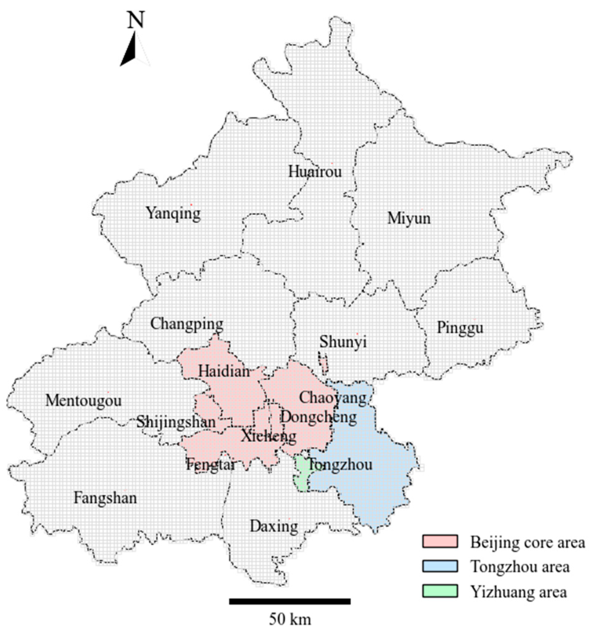
Figure 1. The study area.
Ijgi 14 00487 g001
Figure 2. Selected extreme commuting statistics.
Ijgi 14 00487 g002
Figure 3. Workflow of this study.
Ijgi 14 00487 g003
Figure 4. The distribution of the E C S index.
Ijgi 14 00487 g004
Figure 5. The distribution of local R2 of the GWRF.
Ijgi 14 00487 g005
Figure 6. Global relative importance of variables from the SHAP model.
Ijgi 14 00487 g006
Figure 7. Spatial distribution of the relative SHAP importance of the variables in the generation scenario.
Ijgi 14 00487 g007
Figure 8. Spatial distribution of the relative SHAP importance of the variables in the attraction scenario.
Ijgi 14 00487 g008
Figure 9. Nonlinear effects on extreme commuting generation in the core area.
Ijgi 14 00487 g009
Figure 10. Nonlinear effects on extreme commuting generation in Yizhuang, Beijing.
Ijgi 14 00487 g010
Figure 11. Nonlinear effects on extreme commuting generation in Tongzhou, Beijing.
Ijgi 14 00487 g011
Figure 12. Nonlinear effects on extreme commuting attraction in the core area.
Ijgi 14 00487 g012
Figure 13. Nonlinear effects on extreme commuting attraction in Yizhuang, Beijing.
Ijgi 14 00487 g013
Figure 14. Nonlinear effects on extreme commuting attraction in Tongzhou, Beijing.
Ijgi 14 00487 g014
Table 1. Description and summary statistics of explanatory variables.
Explanatory VariablesDescriptionMeanMinMaxSD
Built-Environment Factors
RDResidential land use density in each grid (/km2)3.320150.6297.63
CDCompany land use density in each grid (/km2)23.7201953.556807.76
LUMLand use diversity index in each grid0.3900.880.08
LUILand use intensity index in each grid (/km2)125.3905404.97137,290
BABuilding coverage area in each grid (%)88,593.40463,784 7.3 × 10 9
HPAverage house prices in each grid (CNY)53,158.810,558195,481 2.1 × 10 8
SDWhether they have the key primary and secondary schools in each grid0.0201 0.02
DCCDistance to the core center (km)38.790.51128.92570.63
DNSDistance to the nearest subcenter (km)19.490.1197.31274.69
BSNumber of bus stops in each grid2.070429.49
RLDRoad length density in each grid (km)4.59021.9312.07
STNumber of subway stations in each grid0.08060.13
Demographic Factors
YCPercentage of commuters between the ages of 25 and 34 in each grid (%)0.36010.02
MCPercentage of male workers in the total number of workers in each grid (%)0.62010.03
COPercentage of commuters owning private cars (%)0.26010.02
HEPercentage of population with bachelor’s degree or higher (%)0.13010.02
ISMedian income score in each grid2.79150.26
CSMedian consumption score in each grid2.17130.08
Note: Several built-environment variables exhibit right-skewed, heavy-tailed distributions with SDs exceeding their means. This is expected in large metropolitan areas where employment, amenities, and transport supply concentrate in the core and along corridors, while extensive peripheral grids take near-zero values. We therefore retain the original scales to preserve substantive heterogeneity. In particular, the wide dispersion of HP reflects large land-price differentials.
Table 2. Description and summary statistics of explanatory variables.
Explanatory VariablesDescriptionMeanMinMaxSD
ECS_AExtreme commuting severity in each attraction grid849.9050,337.8 6.74 × 10 6
ESC_GExtreme commuting severity in each generation grid637.66030,919.2 2.18 × 10 6
Table 3. Global Moran’s I of the extreme commuting severity.
ScenarioMoran’s IpZ
Generation grid (O)0.2100.00091.783
Attraction grid (D)0.4780.00028.220
Table 4. Estimation results of several models.
ScenarioCoefficientOLSRFGWRGWRF
GenerationR20.410.650.490.68
RMSE300.14271.23197.48186.54
MAE204.23192.73131.21129.87
CVRMSE0.4210.3870.2810.266
NMAE0.2510.2450.1530.149
AttractionR20.390.630.470.71
RMSE494.25413.44486.13427.61
MAE326.70351.35301.27292.72
CVRMSE0.4480.3580.4390.374
NMAE0.3620.3900.2340.224
Note. The coefficients R2 for GWR and GWRF models are the arithmetic mean R2 of local models. RMSE = root-mean-square error; MAE = mean absolute error.
Disclaimer/Publisher’s Note: The statements, opinions and data contained in all publications are solely those of the individual author(s) and contributor(s) and not of MDPI and/or the editor(s). MDPI and/or the editor(s) disclaim responsibility for any injury to people or property resulting from any ideas, methods, instructions or products referred to in the content.