


Abstract
This article presents an approach to extend the capabilities of vat photopolymerization (VPP) 3D printing using a robotic arm, with a focus on robust path planning. The robotic cell consists of a Mecademic Meca500 six-axis robot mounted on a Zaber X-LRQ300AP linear guide. The kinematic chain is inverted to reflect the logic of VPP: the world reference frame is fixed to the robot’s tool (the build plate), while the tool frame is attached to the polymerization zone. A virtual degree of freedom for screen image rotation is introduced, bringing the system to eight degrees of freedom. Inverse kinematics are solved under constraints (pose tolerance, joint limits, collision avoidance, and continuity) and evaluated using multi-criteria metrics: manipulability, normalized joint-limit margin, and positional/angular sensitivity. The algorithm follows a deterministic coarse-to-fine search procedure: discrete sweeping of global part orientations, initial sampling with Halton sequences, abd feasibility filtering on a sparsified trajectory, followed by refinement and multi-criteria ranking. The pipeline successfully discarded infeasible orientations and identified feasible printing trajectories for six of the seven benchmark parts, while the remaining case highlights a limitation that may be addressed in future improvements.
1. Introduction
Robot-assisted vat photopolymerization (VPP) combines the geometric freedom and precision of resin printing with the reachability and dexterity of serial manipulators. This integration enables the manufacturing of conformal geometries (where the exposure plane can tilt or move to match the shape of the part), multi-material workflows, and greater in-line automation capabilities than conventional one-dimensional-movement resin printers can typically offer [1]. However, this flexibility also makes motion planning considerably more challenging: to conform to the part geometry throughout the exposure sequence generated by slicing, the robot must satisfy pose constraints while respecting joint limits, remaining distant from singularities, and avoiding collisions within a confined workspace that includes the resin vat, projector, evolving printed part, and potentially other robots.
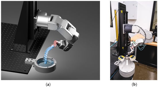
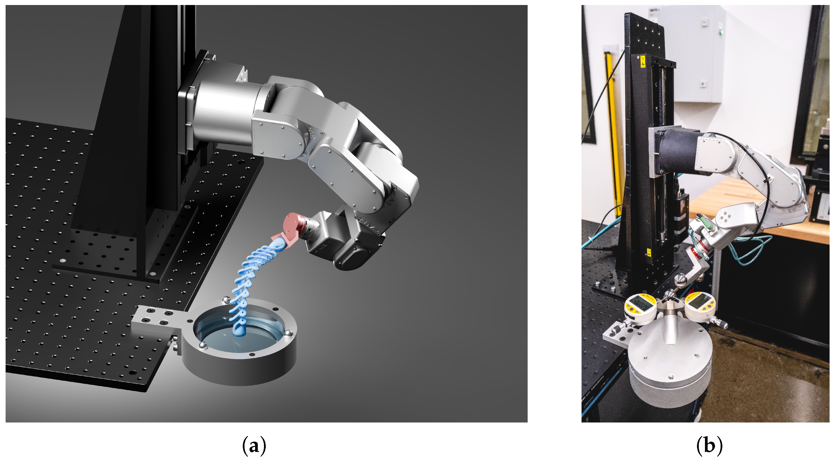
Robot control and robot path planning are two key steps for any robot-operated machining process [2]. Selecting an appropriate global configuration and executing the trajectory pose by pose then become critical to ensuring part quality, process robustness, and cycle time [3,4]. When additional degrees of freedom (DOFs) are added to the six degrees of freedom of the robot arm, as in our system with a vertical linear guide (Figure 1), kinematic redundancies are introduced.
Figure 1.
Overview of the robotic cell: (a) simulation of a printing process and (b) photograph of the physical system during calibration.
At the workcell level, recent surveys in robotic additive manufacturing [5] show growing use of multi-axis and multi-robot setups [6]. These systems operate in a factory environment, where multiple robots share the same workspace. Path planning and collision avoidance are therefore critical to prevent accidents and downtime. Since the robots are part of a production process, planning must be reproducible. The system should produce the same motions each time to facilitate pre-process verifications and ensure consistent quality. These studies focus on FDM, but resin-based processes face the same planning issues. The literature on robotic resin printing is still limited, yet the core constraints and challenges remain the same.
At the controller level, modern real-time inverse kinematics schemes for redundant manipulators explicitly handle joint limits and task priorities while keeping computation predictable [7].
At the same time, learning-based methods aim to generate feasible joint trajectories efficiently. For example, the authors of [8] proposed collective neural dynamics that compute coordinated joint motions for high-DoF arms without relying on full second-order dynamics models.
These methods work well for smooth tracking, but in our VPP cell, we must enforce strict constraints—pose tolerances, joint limits, and collision clearances—at every slice while maintaining continuity during the entire printing process. We also need consistent results across runs. To handle redundancy, we use a constrained solver and a deterministic coarse-to-fine search procedure for feasible path selection in VPP.
Prior work shows that robot-assisted VPP is feasible. Parallel-robot platforms can perform basic tasks but have limited exposure accuracy and photopolymerization control for complex geometries [9,10]. Serial arms have been used to decouple fabrication from single-axis motion and enable conformal, multi-material printing [1]. These systems typically use only a six-DOF arm, demonstrate simpler test parts, and pay limited attention to configuration selection and reproducible search procedures. They also leave open the problem of planning along slice-derived paths under tight kinematic and collision constraints.
The work reported in this manuscript advances the state of the art by (i) formulating VPP as an inverted kinematic problem with the task frame anchored at the exposure contact, (ii) augmenting the system with a virtual screen-rotation DOF (7 + 1 DOFs) to capture projector alignment, and (iii) introducing a deterministic coarse-to-fine search procedure pipeline that combines constrained inverse kinematics (hard pose, limit, and collision margins) with multi-criteria ranking (manipulability, joint-limit margin, and sensitivity).
The pipeline identifies feasible configurations across challenging trajectories with predictable computation and run-to-run reproducibility. This work does not prove that conformal VPP printing with a robot is feasible—Huang et al. [1] already demonstrated this—but it provides a practical tool to convert a resin sliced trajectory for VPP printing (i.e., a series of projected images assigned to poses of the build plate in space) into a robot path plan that respects constraints and redundancy. It enables planning for tightly constrained printing cells while maintaining collision awareness and deterministic outcomes.
For “inverted” tasks—where the environment acts as the tool and the part is carried by the robot—the literature usually expresses constraints in a task-oriented frame using the Task Frame Formalism (TFF) so that constrained and free directions are explicit [3,11]. In this work, we use TFF not to encode force constraints but to decouple projector-related orientation requirements from robot kinematics and to simplify differential kinematics. Concretely, by anchoring the task frame at the exposure (part–vat–window) contact point, the Jacobian needed for pose constraints and small corrective motions is evaluated directly in that frame, which avoids redefining the tool reference frame (TRF) at every printing step and avoids repeated frame-change matrix inversions between tool, world, and projector frames. This reduces implementation complexity and computational cost during slice-by-slice planning. Using the window as the tool reference frame also allows us to apply a standard serial robot model for inverse kinematics. The projected image can be treated as a virtual rotary joint: the window itself does not rotate, but this virtual rotation simplifies the orientation requirements of the printing process and makes planning more straightforward.
Inverse kinematics (IK) methods fall into three families. Closed-form analytical solutions are extremely fast but rely on structural assumptions (e.g., spherical wrist) that are often violated after fine calibration due to numerous non-null dimensions [12,13]. Jacobian-based numerical iterative methods are effective locally and popular in real-time control, yet they handle hard inequalities such as joint limits and clearance margins only indirectly [14,15,16,17]. Optimization-based IK under constraints instead formulates a nonlinear problem with equalities (pose) and inequalities (limits and distances) and has become a de facto standard in modern libraries due to its flexibility [18,19]. In robotized VPP—where safety margins and smooth handover between hundreds of poses are required—the latter is generally preferred.
Beyond local IK, several discrete global decisions strongly condition feasibility and performance: build-plate geometry, the pose of the part on the build plate, and the initial joint configuration (the seed) for trajectory generation. Deterministic low-discrepancy sequences (Halton and van der Corput sequences) provide efficient, bias-free exploration of such decision spaces with far fewer trials and improved reproducibility compared with random sampling [20,21,22]. In additive manufacturing, a coarse discrete sweep over part orientations is widely used to reduce the search space before local refinement [23].
To compare feasible candidates, the community evaluates metrics a posteriori along the path. Three recurrent ones are (i) Yoshikawa’s manipulability, which is used to increase the distance to singularities and improve local motion capabilities [24]; (ii) the normalized margin to joint limits, which not only prevents joint limits but also quantifies the robot’s residual maneuverability; and (iii) pose sensitivity to small joint perturbations, as captured by the differential propagation (), which helps limit error amplification, even away from singularities [25]. Because these metrics are typically non-convex and sometimes conflicting, multi-objective optimization is required [26].
Optimization strategies for competing objectives span from stochastic to deterministic methods. On the stochastic side, simple random or metaheuristic searches, such as simulated annealing, genetic algorithms, and particle swarm optimization (PSO), and evolutionary multi-objective algorithms, such as NSGA-II, explore diverse regions of the search space and approximate a Pareto front, but they are computationally costly and less reproducible due to their use of random seeds, population initialization, and mutation schedules [27]. Previous work using Ant Colony Optimization (ACO) for machining and additive manufacturing demonstrated repeatability in specific scenarios, but this approach remains sensitive to workspace discretization, offers no guarantee of global optimality, and suffers from high computational cost for collision checking and parameter tuning [28]. Other studies in robotized metal additive manufacturing have proposed optimization tools for trajectory planning and kinematic redundancy management but focused on empirical validation (e.g., accelerometer-based behavior analysis) and process-specific criteria, without a general, deterministic framework for constrained, collision-aware planning [29]. A related study showed good results with a PSO algorithm in a work-cell (6R arm + 6-DOF hexapod + 1-DOF rotary table) placement optimization [2], effectively solving 6 + 6 + 1 subproblems rather than a fully coupled 13-DOF search, and without explicit collision checking.
A related class is represented by learning-based planners and controllers—deep reinforcement learning and learned sampling for motion planning—which can discover powerful heuristics but often require substantial training data and careful reward/shaping design and still exhibit variability across tasks and hardware (generalization to a different robot cell is not guaranteed) [30,31,32]. In our VPP setting, where geometric clearances are tight and failures are costly, we observed that stochastic and learning-based approaches were too unpredictable for routine use and difficult to reproduce faithfully across runs and setups.
As a practical alternative, we propose a deterministic, reproducible, and computationally economical pipeline that (i) performs a coarse, discrete sweep over global choices (here, in-plane part orientation); (ii) uses deterministic low-discrepancy seeding to initialize robot joint configuration without bias; (iii) applies a fast feasibility filter on a sparsified path under hard constraints (joint limits and collision margins) using constraint-aware IK; and (iv) fully evaluates all feasible candidates and ranks them by aggregated metrics specially chosen for VPP (manipulability, joint-limit margin, and sensitivity) via scalarization or Pareto reporting [18,26,33]. Crucially, we formulate the problem in a task-oriented frame anchored at the exposure contact, which cleanly separates process-driven orientation requirements from robot kinematics and simplifies differential kinematics (Jacobians are evaluated directly in the task frame, avoiding repeated frame changes). Unlike approaches that decompose redundancy or freeze subsets of joints, every IK solverin our pipeline performs a full eight-DOF configuration search simultaneously—coupling the linear rail, the six-DOF arm, and the virtual screen rotation—thereby avoiding inconsistencies from staged/partial search and improving feasibility and smoothness along the entire trajectory.
This design is tailored to robot-assisted VPP: early filtering removes infeasible orientations before costly evaluation; deterministic seeds and solvers keep the computational cost predictable and the results reproducible; and the ranking step makes the trade-offs between manipulability, joint-limit margin, and sensitivity explicit. In short, the pipeline favors predictability and transparency—two properties essential in a safety-critical, tightly constrained printing cell. Since the robot operates at moderate speeds and the manipulator is rarely close to kinematic limits, our goal is to find a feasible and sufficiently good configuration that stays away from singularities rather than to explicitly optimize manipulability. This simplification reduces computational cost without affecting trajectory quality for VPP.
The printing process studied in this manuscript proceeds as follows. First, a 3D part is designed in CAD software. While robot-assisted VPP allows for more complex curves, the part must still meet manufacturability requirements for VPP, such as limited cavities to prevent liquid resin from being trapped. Then, the part has to be sliced: a series of planes is defined along a sweep curve that approximates the shape of the CAD model. Each plane is offset from its neighbor by a small distance, called the printing resolution, and tilted at a small angle. Both the distance and angle are chosen to avoid collisions between the already printed layers and the bottom window. Once all planes are defined, a series of images is generated by slicing the CAD part and keeping the solid sections. These images will be sent into the projector to polymerize specific areas for each printing layer. Finally, the method described in this manuscript uses each step of the curve and translates it into a pose in space (positions and orientations with respect to the first layer, the z-component of which corresponds to the plane normal used for slicing). These poses are then used for the inverse kinematics computation between the reference frame (the build plate mounted on the robot) and the tool frame (the virtual image projected at the bottom of the printing vat). Once the robot’s path is selected, the printing process begins: the robot reaches the first printing position (the build plate is nearly in contact with the vat window), and the corresponding image is projected during a brief moment to allow the resin to polymerize. After exposure, the robot raises the part slightly to separate the newly cured layer from the vat window before moving to the next layer. At the end of the printing phase, the robot uses the pneumatic tool changer to place the build plate on a support, such as the one displayed in Figure 1 of [34]. An empty build plate can then be attached to print either the same or another part.
On a set of seven representative sliced trajectories, the pipeline detects infeasible options early, then selects print configurations that balance manipulability, joint-limit margins, and sensitivity better than naïve orientation/initialization choices. In six of seven benchmark parts, it delivered feasible printing trajectories with predictable compute and identical results across repeated runs. The selected trajectories were executed on the experimental robotic cell shown in Figure 1b to validate the kinematic feasibility and geometric constraints of the proposed path-planning approach within the context of the VPP printing process. This process imposes specific constraints that are critical for ensuring the theoretical viability of the trajectories prior to material deposition. Note that runs were conducted without resin exposure, focusing on the validation of the trajectory-planning framework rather than the static response of the robot, which is highly system-dependent and difficult to generalize across different robotic platforms. The remaining case highlights a current limitation—an instance where no feasible trajectory was found under the imposed constraints—which may be addressed by future extensions (e.g., broader orientation search, additional slack in free rotations, or richer feasibility heuristics).
In summary, we place configuration search and optimal selection at the core of VPP planning: modeling at the right level, guarantee of local feasibility, and global decision making through multi-criteria evaluation. In Section 2, we detail the robotic cell, the inverted-chain system model, the constrained IK formulation, the collision model, the evaluation metrics, and the deterministic coarse-to-fine optimization pipeline (with parameter settings for reproducibility). Section 3 presents the experimental results obtained on four benchmark parts. Section 4 discusses the implications, limitations, and possible extensions of this work, and Section 5 concludes the paper. Table A1, Table A2, Table A3, Table A4, Table A5, Table A6, Table A7 and Table A8 provide per-angle summaries.
2. Materials and Methods
2.1. Robotic Cell and Software Stack
The printing cell consists of a serial 6-DOF robot (Meca500 from Mecademic, Montreal, QC, Canada) mounted on a vertical linear guide (X-LRQ300AP from Zaber, Vancouver, BC, Canada), yielding seven physical DOFs. The resin vat and DLP projector form the exposure subsystem. A virtual eighth degree of freedom models the in-plane rotation of the projected image (screen rotation about its normal). Calibration (geometric and elastic) is assumed to be available from prior work [34,35]. The robot’s architecture and linear guide follow the same configuration as in that work, and the Denavit–Hartenberg parameters are identical to those reported there. Accordingly, realistic forward and inverse kinematic models of the robot chain are used here in place of the nominal models.
For modeling and simulation, the complete robotic cell was reconstructed in Blender (version 5), including both visual meshes and collision proxies, and a URDF of the inverted kinematic chain was exported using Phobos. Collision checking operates on simplified primitives (boxes, cylinders, and spheres) that conservatively approximate the visual meshes. All optimization and kinematic routines were implemented to use the URDF model directly. To maintain consistency between the digital and physical robot, the URDF can be updated automatically from calibration data by editing a set of approximately 80 parameters (link lengths, offsets, and joint frames).
2.2. System Model
In projection-based VPP, the environment (projector and resin vat) remains fixed in the world, while the printed part is carried by the robot. Most robotic simulation frameworks, however, define the robot’s tool reference frame (TRF) as the active end effector and keep the workpiece stationary. To match the physics of the process, we therefore model an inverted kinematic chain: the world frame is fixed to the robot flange, and the tool frame is fixed at the vat window. This inversion has two key advantages: (i) trajectories produced by slicing (poses of the part relative to the vat) map directly to end-effector targets without per-step matrix inversions, and (ii) task-space quantities can be evaluated at the exposure contact point, which is the physically relevant location for constraints. We assume slicing has already been performed, taking the surface normal tangent to the curve, and do not address material deposition or fill patterns, which are important but out of scope for this robotics-focused study.
The task frame is anchored at the part–vat contact (exposure) point, and pose constraints are expressed in that frame. Evaluating the translational and rotational Jacobians, i.e., and , at this location avoids redefining the TRF at every slice and removes repeated frame transformations between the tool, world, and projector frames. It also preserves the correct differential coupling between small orientation errors and linear deviations at the front of the part, which would otherwise be underestimated if computed at the nominal TRF as the printed part grows layer by layer.
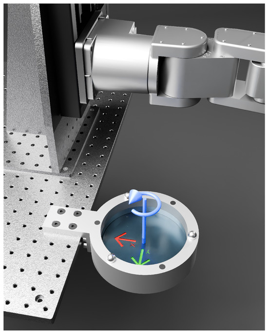
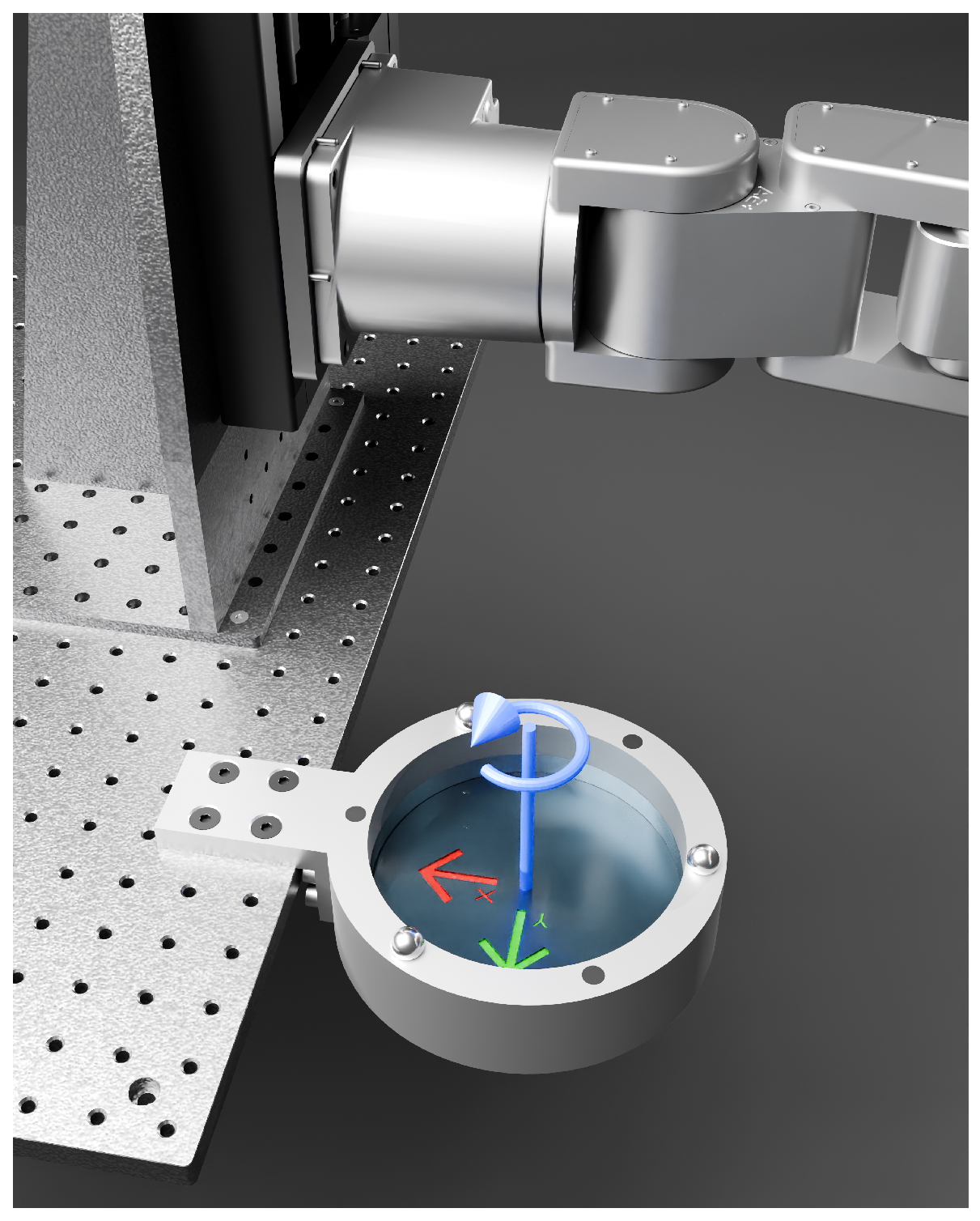
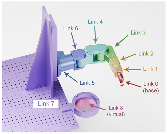
The screen’s in-plane image rotation is modeled as a revolute joint located at the center of the vat and aligned with the screen normal (Figure 2). This choice reflects the assumption that printing occurs near the vat center, where the projected image can only rotate about its optical axis. In principle, planar translations between layers could also be modeled, but doing so would introduce two additional degrees of freedom and significantly complicate the inverse kinematics, with little expected benefit in terms of trajectory feasibility.
Figure 2.
Virtual degree of freedom (in blue) modeled as a revolute joint added to the kinematic chain of the serial robot.
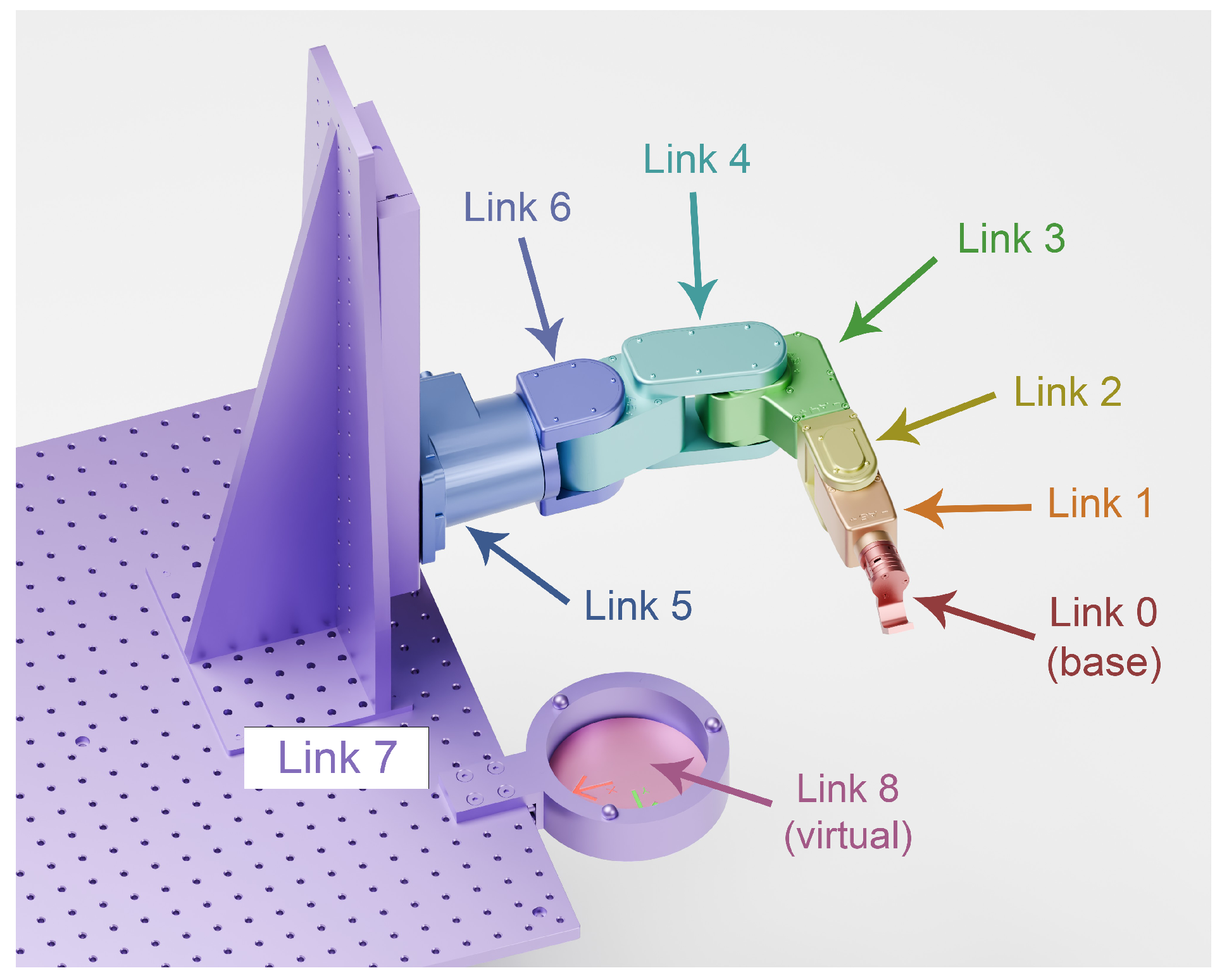
This virtual joint carries the commanded image angle () returned by the IK; it adds no inertia or limits to the model. With this addition, the chain has eight DOFs (seven physical and one virtual; see Figure 3).
Figure 3.
Inverted kinematic chain of the robotized VPP system. A joint is modeled between each link, resulting in a total of eight degrees of freedom.
Importantly, the virtual joint does not introduce any risk of discontinuity and cannot be used to generate discontinuity. This is because the printed trajectory is continuous: the kinematic chain is closed by the part currently being printed. In other words, with continuous printing, the only way to produce a discontinuity at joint 8 would be to induce a discontinuity at another joint of the chain. Since the other joints are physical and constrained by mechanics, such discontinuities are impossible during normal operation. Therefore, the virtual joint simply tracks the commanded image angle, without affecting the continuity or feasibility of the motion.
2.3. Reference Parts and Trajectories
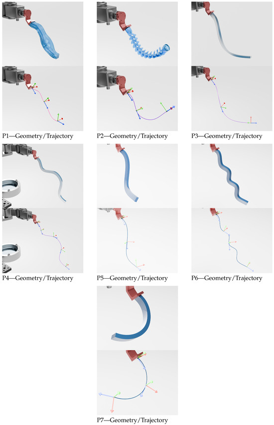
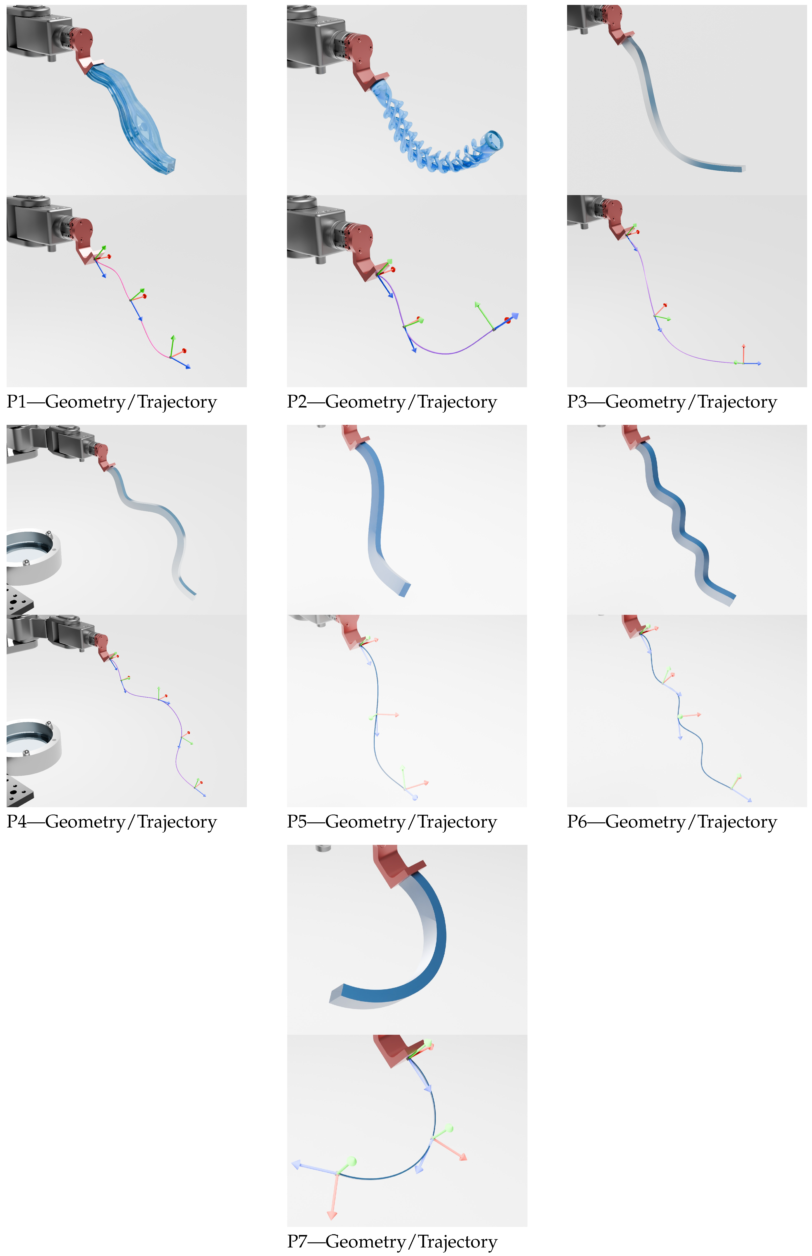
To exercise diverse geometric conditions, we use seven reference parts (P1–P7) from 2D curves to more complex 3D paths. The slicing-generated exposure paths define the target pose sequence () in the task frame. Table 1 summarizes the dimensions and path length, and Figure 4 shows each geometry (left) and its trajectory (right). The last column (Total Absolute Curvature or TAC) is used as a complexity criterion for printing, alongside path length. TAC is a well-known measure in differential geometry that quantifies the total amount of bending along a curve [36], providing insight into the geometric complexity and the difficulty of following the path with a robot or printer. Higher TAC values indicate more complex, highly curved trajectories, which typically require more precise control and can increase the risk of errors or instabilities during printing.
Table 1.
Reference parts used for evaluation: bounding-box dimensions, total path length, and total absolute curvature.
Figure 4.
Overview of the seven reference parts (P1–P7). The geometry (top) and planned printing trajectory (bottom) are shown for each part.
2.4. Collision Modeling
Collision checks are performed between a selected set of robot–environment pairs with a signed distance of . We enforce a conservative clearance of using primitive proxies, where represents the minimum allowable distance between objects; adjacent or rigidly connected links are excluded from self-collision tests. Unless otherwise stated, .
2.5. Constrained Inverse Kinematics (IK)
Let be the forward kinematics homogeneous matrix, and let the target sequence of N poses be with .
Let be the joint-space norm that measures the “distance” between two joint configurations. It is defined by , where the diagonal weighting matrix () homogenizes scales (rotary vs. prismatic) and can encode joint-motion preferences.
For each , we solve for :
where is the norm of the positional difference and denotes the geodesic rotation error (angular difference) between the rotation matrices ( and ).
Note that contains both revolute (radians) and prismatic (meters) joints. Therefore, the joint-space norm () combines quantities with different units. The weighting matrix () is a diagonal matrix used to balance revolute and prismatic joint contributions. In this work, it is defined using simple unit-based scaling so that angular joints (radians) and linear joints (meters) have comparable magnitudes. No task-dependent tuning is applied, and is fixed across all experiments.
In this problem, minimizing the quadratic term () biases the solution toward the previous configuration to promote continuity and avoid branch switching. This soft penalty complements the hard trust-region constraint that caps per-step joint changes. The choice of the initial joint configuration () is detailed in Step 2 of Section 2.7.
2.6. Evaluation Metrics for Trajectory Ranking
Metrics are computed a posteriori on feasible trajectories, with Jacobians evaluated at the task frame (exposure contact).
- (i)
- Yoshikawa manipulability.
Translational and rotational manipulability are
For a trajectory, we take the minimum along the path: and , where higher values indicate better dexterity and distance from singularities.
- (ii)
- Normalized margin to joint limits.
For joint i with bounds ,
with being the minimum value among all joints and being the minimum value along the entire trajectory. This also serves as a proxy for residual maneuverability (headroom for additional motions such as a peel/detachment routine at the end of printing).
- (iii)
- Pose sensitivity to small joint errors.
Let model the expected joint position variances, where is the standard deviation of joint i (radians for revolute and meters for prismatic). The propagation of joint errors to task space is modeled using first-order kinematics [3].
First-order kinematics map these joint errors to task-space errors via the following Jacobians:
where and are task-space covariance matrices. Their diagonal entries give the variance of the position and orientation errors, respectively, along each Cartesian axis, while the off-diagonal entries represent the covariances between errors along different task-space axes, reflecting kinematic coupling introduced by the Jacobian. For simplicity, we reduce each matrix to a scalar score by summing the diagonal terms (trace), giving the total expected variance along all axes [37].
with lower values meaning “less amplification” of joint errors. We evaluate their mean along the trajectory.
Its aim is to minimize the expected task-space variance induced by joint perturbations, i.e., it prefers joint configurations that attenuate the propagation of encoder/compliance noise. This criterion favors configurations where the Jacobian’s singular values are small in directions that amplify errors, promoting robustness at the potential cost of dexterity. Unlike Yoshikawa’s manipulability, which maximizes the volume of the manipulability ellipsoid, this trace-based metric minimizes the total task-space variance induced by a model of potential joint errors (encoder noise, compliance, and backlash). It favors configurations where the Jacobian has a globally small magnitude—a condition that does not coincide with singularities, where only select task-space directions lose amplification, while column norms may remain large.
2.7. Deterministic Coarse-to-Fine Search Pipeline
We select (i) a global in-plane rotation () of the part about the screen normal and (ii) an initial joint configuration (seed) to roll out the constrained IK over the full pose sequence. To control cost and improve reproducibility, we use the following staged procedure:
- Step 1—Discrete sweep of global orientation.
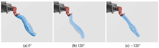
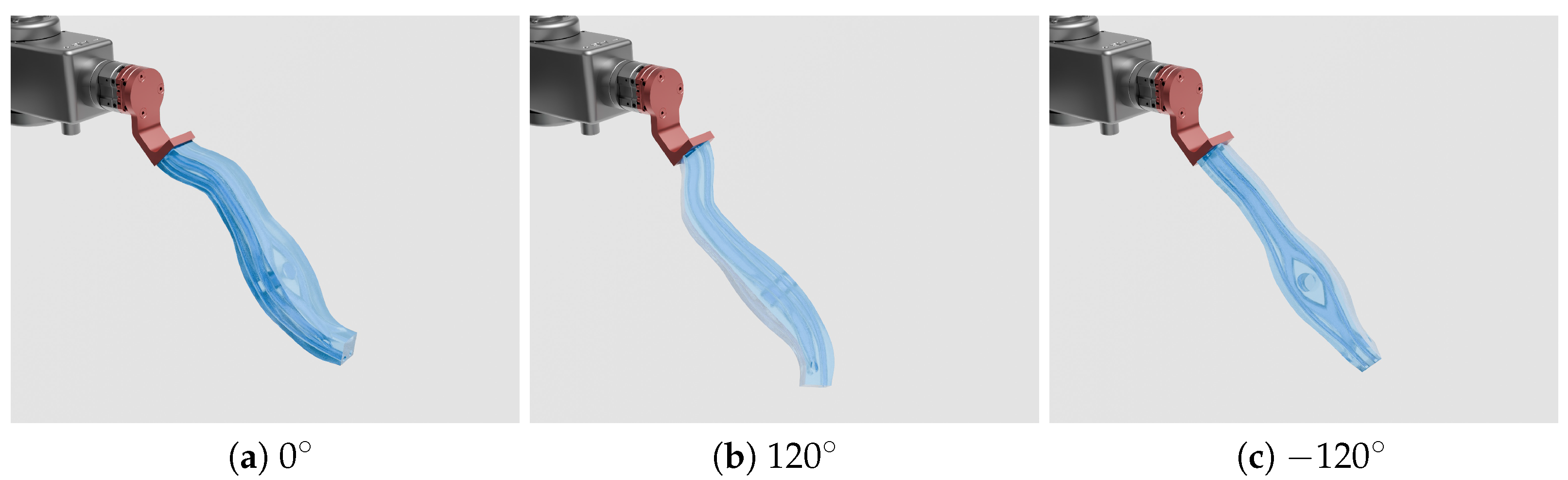
We discretize into equally spaced angles over , with a step of (in our experiments: , ). We then rotate all target poses as (examples in Figure 5).
Figure 5.
Examples of global part rotations for P1: (a) 0, (b) 120°, and (c) −120°. These correspond to discrete in-plane orientation samples.
- Step 2—Deterministic seeding of initial joint configurations.
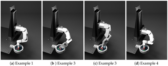
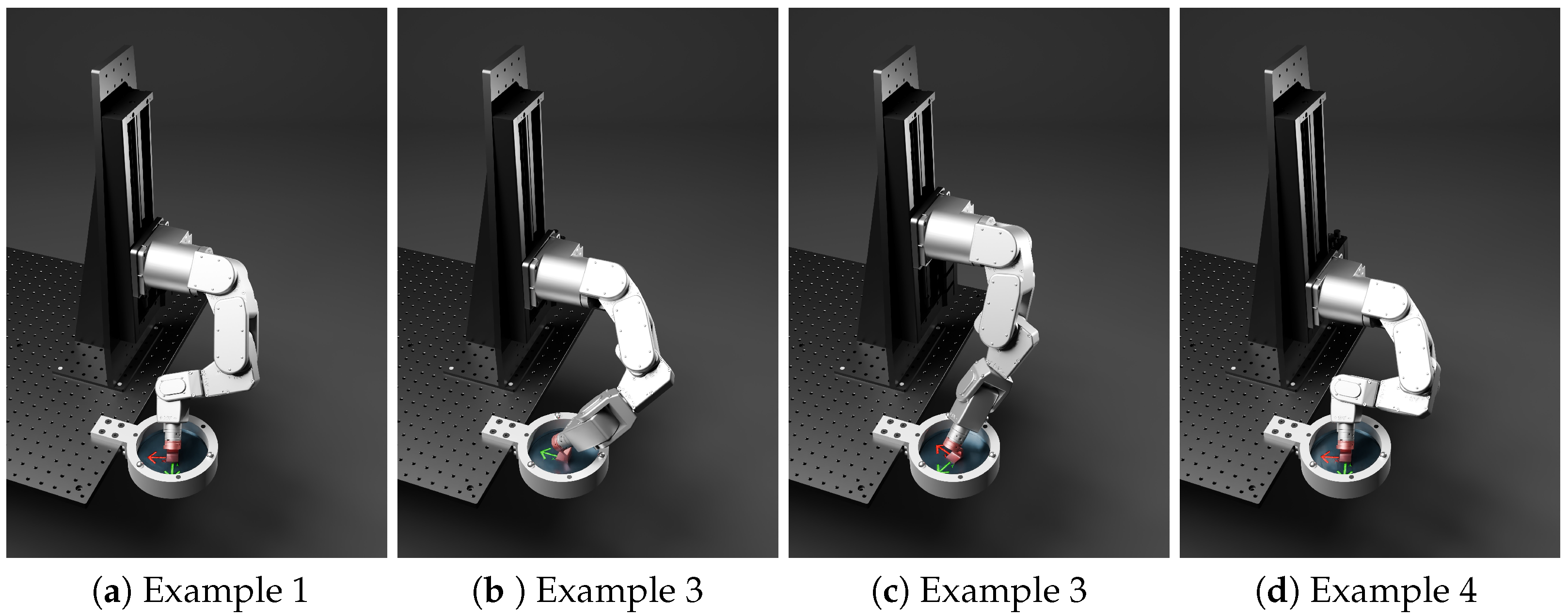
For each orientation (), we generate initial joint configurations () using a low-discrepancy sequence (e.g., Halton) within , then solve a single-pose IK to anchor trajectory generation (examples in Figure 6). (In our experiments: .)
Figure 6.
Four examples of initial printing joint configurations for a global part rotation of 0°.
- Step 3—Fast feasibility filter on a sparsified path.
Using a stride of s (every s-th pose), we attempt a constrained IK evaluation per seed and early exit on the first violation (limits, pose, and collision). Surviving candidates receive a coarse score; we keep the best 12 per .
- Step 4—Refinement on the full path.
The selected 12 candidates are recomputed with a stride of 1, full constraints, and continuity regularization.
- Step 5—Multi-criteria evaluation.
Each refined trajectory is scored using the metrics mentioned above (manipulability minima, joint-limit margin minimum, sensitivity means, and optional extras such as joint-space length or smoothness). The joint-space length measures the total distance traveled by all joints along the trajectory:
where is the vector of joint positions at step t, containing both revolute (radians) and prismatic (meters) joints. The weighting matrix () is defined in Section 2.5. Lower values indicate more direct and efficient motion.
Smoothness is defined using a discrete second-order difference along the joint sequence:
This term corresponds to a second-order finite difference without time normalization. It does not represent a physical acceleration. Instead, it measures variations in joint velocity between successive discrete steps. High values indicate sharp changes in velocity. Low values indicate smoother motion along the planned sequence.
- Step 6—Selection (and optional windowed rescan).
For each metric, values are normalized between 0 and 1 using min–max scaling across all candidate trajectories:
where is the raw metric value for a trajectory and and are the minimum and maximum values of this metric over all candidate trajectories. Metrics to maximize are scaled inversely so that a higher value is always better.
Normalized metrics are aggregated into a single score for each trajectory using a weighted sum:
where is the weight assigned to metric i. Trajectories that violate constraints receive strong penalties. The trajectory with the highest aggregated score is selected as the best candidate.
Alternative aggregation methods exist, such as the Tchebychev distance-based approach, which evaluates trajectories based on their worst normalized metric. Although not used here, it could be interesting to study its impact on trajectory selection in future work.
Finally, we return the best according to the global score. If no feasible trajectory is found after the initial sweep, we optionally rescan a restricted angle window for Step 1 around the most promising coarse region, then repeat Steps 1–5 once.
3. Results
The seven benchmark parts are shown in Figure 4; their main geometric properties are summarized in Table 1. A video illustrating the execution of the selected candidate trajectories for six of these parts is available at https://youtu.be/XPKsUUgA1AQ, accessed on 21 April 2026.
We sweep the in-plane part orientation on a uniform grid: we use , so . For each angle, we generate 100 initial joint configurations from a low-discrepancy (Halton) sequence and run a coarse feasibility test on a sparsified trajectory (stride of ) with early exit at the first constraint violation.
Hard constraints include joint limits, pose tolerances , and a collision clearance of . A trust region limits per-step joint changes to ≈2–3 mm and ≈1° during the coarse pass and is tightened (0.1–0.2 mm) for refinement.
Each trajectory is scored by combining multiple metrics with assigned weights. The chosen weights are arbitrary and serve to balance the influence of each metric in the aggregated score. For translational and rotational manipulability minima, the weights are and , respectively. The joint-limit margin is weighted 0.5. Positional and rotational sensitivity means are weighted 1.0 each. Optional metrics include the joint-space path length (L), which is weighted 0.1, and discrete smoothness (S), which is weighted 0.05.
The top 12 seeds per angle are then recomputed pose by pose on the full path under the same constraints. When no refined solution is found in the first pass, a second pass rescans a ±15° window around the most promising coarse angle. No stochastic components are used; given identical inputs, the pipeline produces identical outputs. Metric definitions, tolerances, and clearance margins appear in Section 2; per-angle summaries are reported in Table A1, Table A2, Table A3, Table A4, Table A5, Table A6, Table A7 and Table A8.
3.1. Feasibility Versus Orientation and Compute Cost
3.1.1. Feasibility Maps
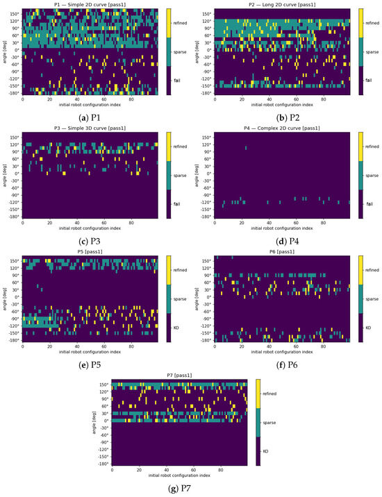
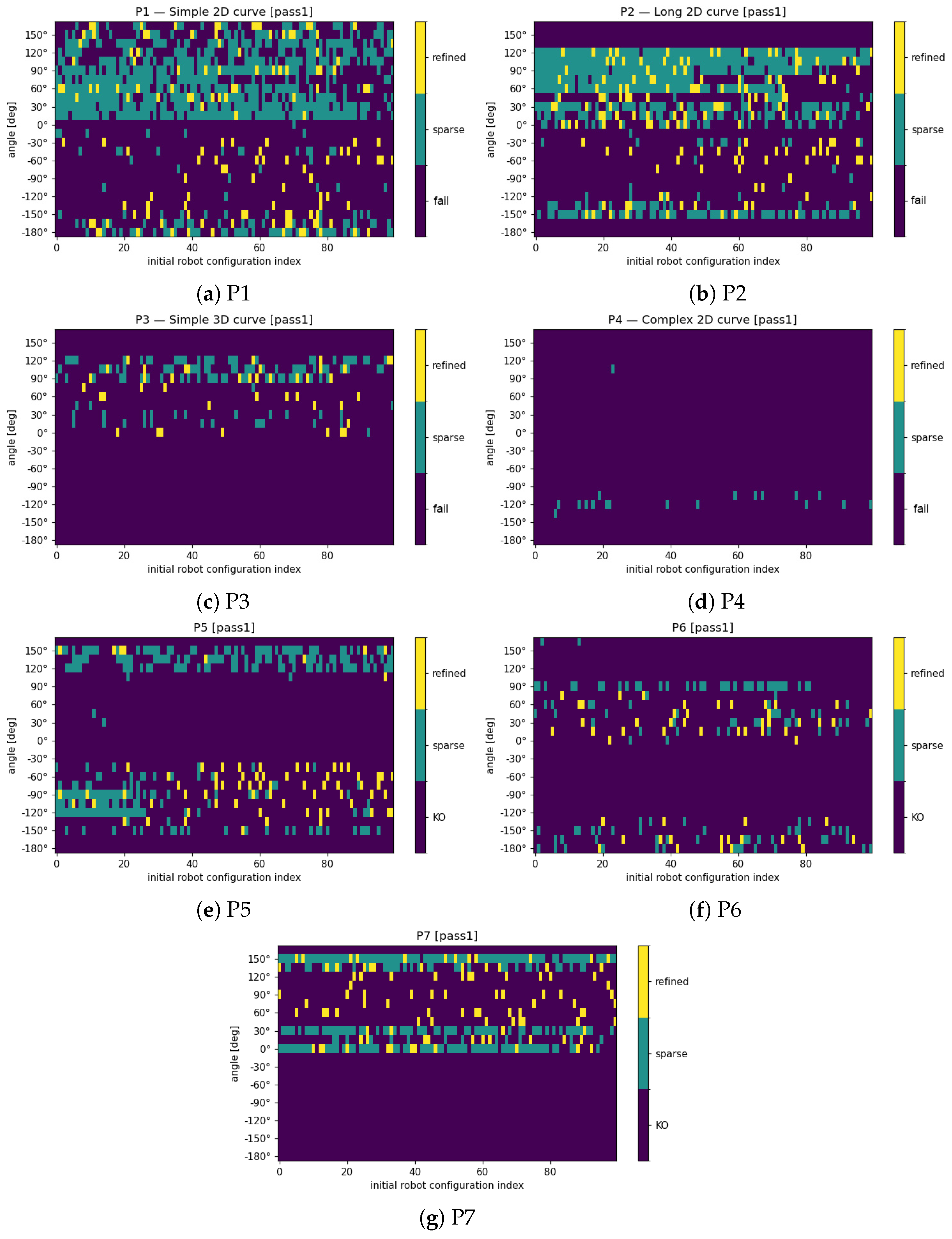
Figure 7 contrasts coarse-feasible (turquoise) and refined (yellow) solutions across orientation and seed index. Two consistent trends emerge:
Figure 7.
Feasibility maps for the seven benchmark parts (P1–P7) as a function of the part’s in-plane rotation angle and initial joint configuration. Turquoise: coarse-feasible candidates; yellow: fully refined, constraint-satisfying trajectories.
- Orientation is decisive. Entire angular ranges are infeasible, while others concentrate most solutions. For P3, feasibility clusters between roughly 0° and 135°. P6 presents two clusters around 60° and −180°. A single cluster is clearly visible for P7, where every solution is bound between 0° and 150°.
- Task difficulty aligns with expectations. The density of feasible points appears to decrease when the total absolute curvature (TAC) increases and the trajectory length is significant. Smaller trajectories with a high TAC, like P6, seem more accessible in our case. This, however, may vary depending on the robotic system used and the placement of the cell.
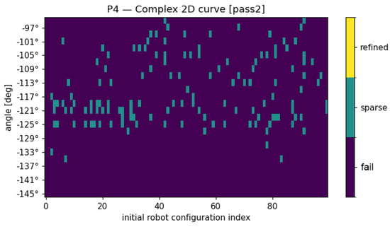
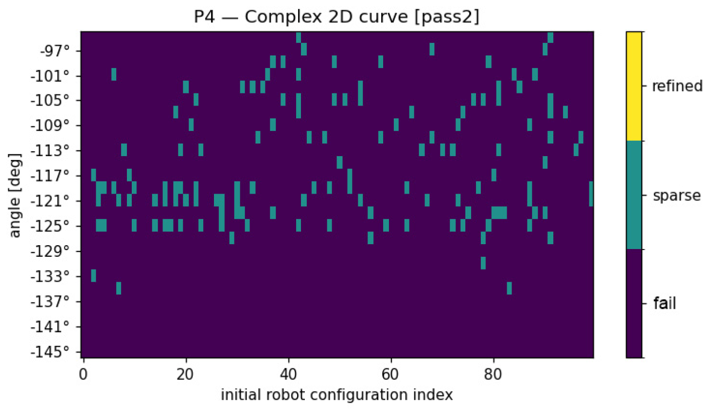
For P4, a second pass restricted to a ±15° window uncovers additional coarse-feasible candidates but still yields no fully refined trajectory (Figure 8). The main cause is the inverse-kinematics solver failing under the joint-limit proximity constraint: although a solution exists in isolation, it is unreachable from the previous joint configuration due to the limited motion allowed between consecutive slices. Other contributing factors may include insufficient seed diversity at useful angles or the geometric complexity of the part relative to our cell.
Figure 8.
Feasibility map for part P4 in the second (refined) pass, restricted to a narrower angular window around the most promising orientations. Turquoise: coarse-feasible candidates; yellow: refined feasible trajectories (none found in this case).
3.1.2. Compute Time per Angle
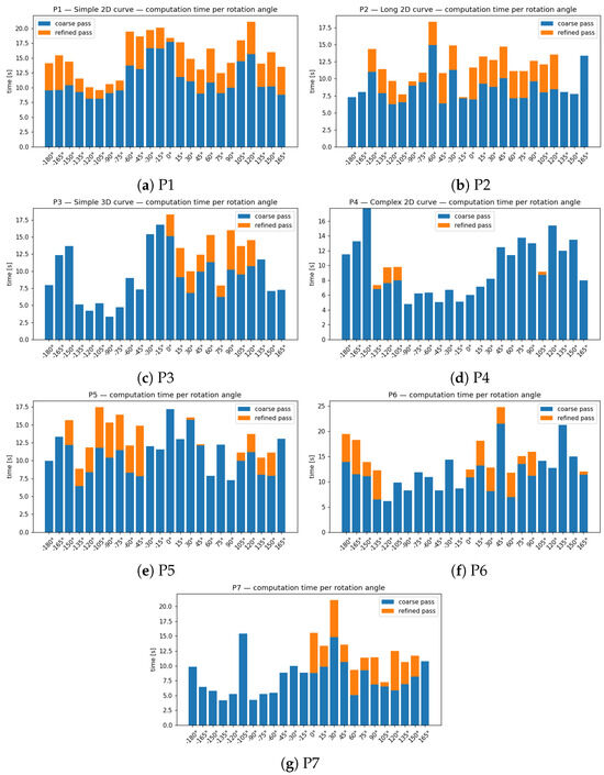
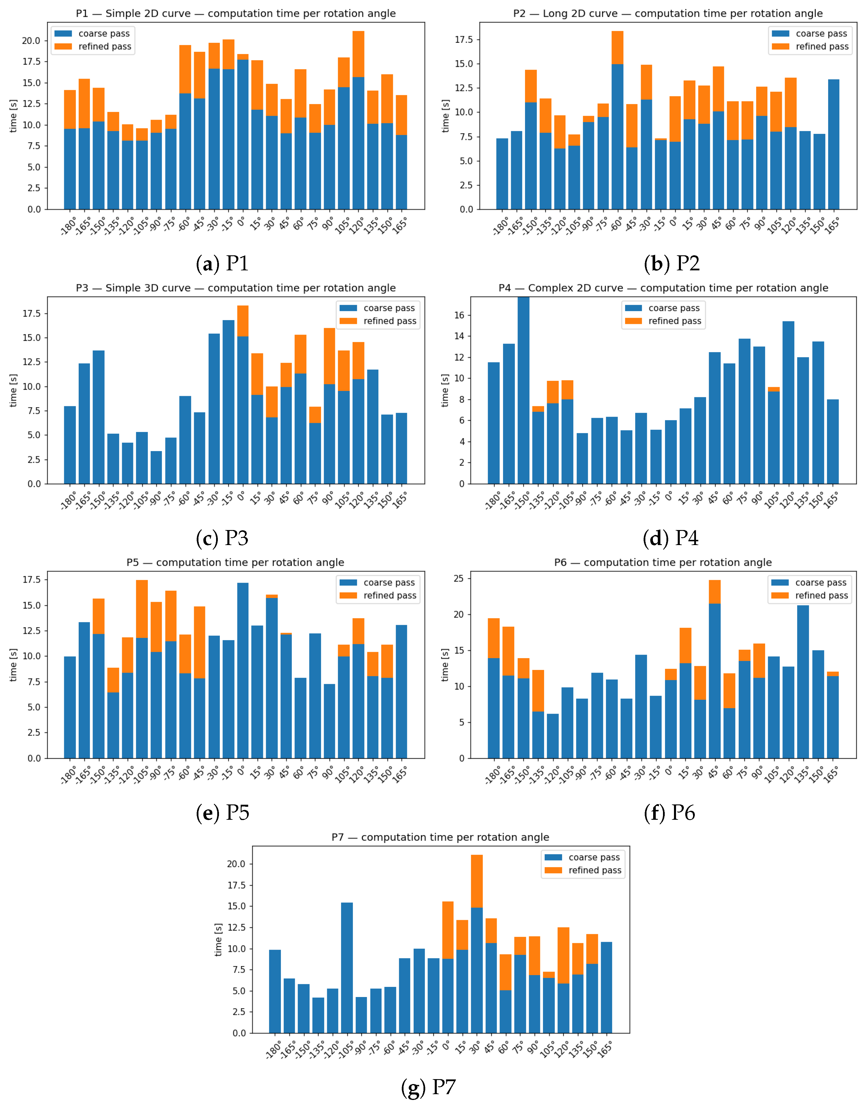
Figure 9 reports stacked computation times (coarse at the bottom, refined on top). Two regimes appear:
Figure 9.
Computation time per rotation angle for each benchmark part (P1–P7). Each bar shows total computation time per angle, split into coarse-stage (blue) and refined-stage (orange) contributions. The coarse stage is executed for all seeds, while the refined stage is applied only to selected candidates that pass the coarse filtering step. Sterile angles yield only coarse evaluations. Promising angles show higher refinement cost due to full trajectory validation. The x-axis corresponds to the rotation angle of the platform in degrees.
- Sterile angles: few or no coarse survivors (refine time negligible);
- Promising angles: multiple seeds reach refinement, increasing time but producing validated full trajectories.
The coarse stage is executed for all seeds, while the refinement stage is executed only for selected candidates that satisfy the coarse criteria. Thus, the coarse stage reduces computation by filtering out unfavorable orientations. Higher refinement cost at promising angles reflects the number of validated trajectories rather than a per-evaluation cost increase.
3.2. Refinement and Multi-Criteria Evaluation
For each angle, the top 12 seeds are refined along the full trajectory and scored with manipulability (positional () and rotational ()), normalized joint-limit margin, and sensitivity, as defined in Section 2. Aggregated results (see Table A1, Table A2, Table A3, Table A4, Table A5, Table A6, Table A7 and Table A8) show the following:
- P1 (2D simple curve): Several angles reach refine_ok = 12 (−180° to 165°); best scores near −45° and 45–60°;
- P2 (2D long curve): Dense feasible region for [0°, 120°] with robustness peaks at 60°;
- P3 (3D simple curve): Active window [0°, 120°]; best score near 60°;
- P4 (2D complex curve): No fully feasible trajectory in either pass;
- P5 (3D simple curve): Main feasible window in the negative range [−135°, −45°], with a robustness peak at −75° where 12 initial joint configurations out of the 12 selected joint configurations resulted in a success; secondary and weaker feasible cluster around 135°–150°; no solution near 0°;
- P6 (3D complex curve): Two separated feasible bands—one around [−180°, −135°] (best score at −165°) and another around [0°, 60°]—with a robustness peak at 0° (highest score overall); large infeasible gap between −120° and −15°;
- P7 (2D simple curve): Broad positive feasible region [0°, 150°] with multiple fully feasible angles; strongest robustness at 60° and high seed density at 150°; no feasible solution for negative angles.
Table 2 lists the champion configuration per part (orientation (); seed index; best score; and minima of , , and joint-limit margin). All winners lie in the promising orientation bands identified earlier, validating the coarse-to-fine design. The minimum joint-limit margin () indicates that at least one joint reaches its limit momentarily—often the linear rail—which should be monitored experimentally.
Table 2.
Champion configurations per part. , : positional and rotational manipulability; : minimum normalized joint-limit margin along the trajectory; , : positional and rotational sensitivity.
4. Discussion
This work investigated a deterministic, coarse-to-fine pipeline for finding a reliable printing configuration in robot-assisted vat photopolymerization (VPP). The approach integrates an inverted kinematic chain (vat window as end effector), a virtual screen-rotation degree of freedom, constrained inverse kinematics (IK) with hard limits (pose, joint ranges, and collision margins), and deterministic exploration (angular sweep + low-discrepancy seeding), followed by multi-criteria ranking (manipulability, joint-limit margin, and sensitivity).
Across the seven benchmark parts, the results highlight three points. First, global orientation strongly conditions feasibility: solutions concentrate in “orientation bands”, whereas large angular intervals contain no valid trajectories. Second, early feasibility checks on a sparsified trajectory effectively prune sterile regions, keeping compute time predictable while preserving promising candidates for refinement. Third, when feasible, the pipeline typically yields several high-quality options whose trade-offs are explicit in the scalarized view (Table A1, Table A2, Table A3, Table A4, Table A5, Table A6, Table A7 and Table A8). These observations align with the design goals stated in the Introduction: predictable performance, reproducible exploration, and transparent decision criteria in an industrial robotic cell.
Limitations follow naturally from the problem structure. Feasibility depends on the discretization of the angular sweep; compute scales with trajectory length and the number of seeds taken to refinement; and joint-limit margins can be locally tight when workspace clearances are tight. The failure on P4 indicates that some geometries remain outside the feasible set under current constraints. Practical extensions include (i) local continuous orientation optimization around favorable angles; (ii) adaptive stride on the sliced path (coarser where constraints are loose and denser near tight clearances); (iii) null-space biasing, which exploits the redundancy of the eight-DOF chain to project secondary objectives (e.g., joint-limit margin maximization) into the Jacobian null space, improving joint configuration quality without affecting end-effector pose, or adaptive joint weights, where the diagonal entries of W are updated along the trajectory to penalize joints approaching their limits more heavily, providing a continuous margin-preserving behavior; and (iv) coupling the per-step IK solver with a look-ahead motion planner to guard against long-horizon infeasibility (since each IK solution implicitly constrains the reachable set of future configurations, a locally valid solution can propagate by continuity into a dead end where no subsequent configuration satisfies both pose and collision constraints simultaneously; a global planner operating over the full trajectory horizon would anticipate such failure modes and reject branching decisions that, while locally feasible, lead to inevitable future collisions or joint-limit violations); and (v) integrating a peel/delamination micro-motion criterion relevant to VPP.
Looking ahead, three extensions merit attention. First, a deeper analysis of the P4 failure could help pinpoint root causes—by monitoring the feasibility at each layer, tracking active constraints, examining clearance margins, and monitoring joint-limit proximity—to assess whether infeasibility comes from orientation gaps, narrow passages, or sustained limit saturation; such insights could guide targeted local orientation refinement and constraint tuning. Second, the benchmark could be broadened to a larger, more demanding panel of parts to stress generality. Third, head-to-head comparisons with stochastic/evolutionary baselines (e.g., PSO and NSGA-II) under identical constraints and compute budgets could be conducted, reporting the success rate, best/median score, runtime, and run-to-run variance; hybrid variants—stochastic warm-starts followed by constrained IK refinement—could also be explored.
5. Conclusions
We presented a deterministic path-planning framework for robot-assisted VPP that (i) models the process with an inverted chain and a virtual screen-rotation DoF; (ii) enforces feasibility through constrained IK with explicit limits and collision margins; (iii) reduces search cost via a coarse angular sweep and deterministic seeding; and (iv) ranks feasible trajectories using manipulability, joint-limit margin, and sensitivity. On six of seven benchmark parts, the method identifies at least one feasible and well-scored trajectory; it also isolates the orientation bands where solutions concentrate, providing actionable guidance for setup.
Although this study did not test physical printing, it demonstrates a method for finding valid configurations and selecting the best configuration specialized for VPP, laying the groundwork for future work on physical implementation.
The study highlights practical implications: it enables predictable trajectory generation, transparent decision making in safety-critical setups, and early pruning of infeasible regions, which are crucial for planning in complex VPP geometries.
Limitations are acknowledged: feasibility depends on angular discretization, joint-limit margins can be tight in constrained workspaces, and some geometries (e.g., P4) remain infeasible under current constraints. These observations motivate targeted improvements in local orientation refinement, adaptive path sampling, and hybrid motion planning strategies.
Future work will expand the benchmark set to test generality, incorporate head-to-head comparisons with stochastic/evolutionary baselines (PSO and NSGA-II), and explore hybrid variants combining deterministic IK refinement with stochastic warm starts. Logging of per-slice feasibility and constraint activity can further guide automated trajectory adaptation and constraint tuning.
Overall, the presented framework provides a structured, reproducible, and transparent approach to robot-assisted VPP path planning, offering a foundation for both practical deployment and further research in constrained robotic additive manufacturing.
Author Contributions
Conceptualization, E.R., I.A.B., E.J., P.Z., C.S. and N.Z.; methodology, I.A.B.; software, E.R.; validation, E.R.; formal analysis, E.R.; investigation, E.R., E.J. and P.Z.; resources, E.R. and I.A.B.; data curation, E.R.; writing—original draft preparation, E.R.; writing—review and editing, I.A.B., C.S. and N.Z.; visualization, E.R.; supervision, E.R., I.A.B., C.S. and N.Z.; project administration, I.A.B.; funding acquisition, I.A.B. and N.Z. All authors have read and agreed to the published version of the manuscript.
Funding
The authors would like to thank Nissan North America Inc. and Mitacs for funding this research work.
Data Availability Statement
The data presented in this study are available on request from the corresponding author.
Acknowledgments
During the preparation of this manuscript/study, the author(s) used ChatGPT-4 (OpenAI, San Francisco, CA, USA) for the purposes of text editing, including language polishing, grammar correction, and improvement of structure and clarity. The authors have reviewed and edited the output and take full responsibility for the content of this publication.
Conflicts of Interest
The authors declare the following financial interests and personal relationships that may be considered as potential competing interests: Ilian A. Bonev reports financial support provided by Mitacs Canada and Nissan North America Inc. and a relationship with Mecademic that includes equity or stocks. Ilian A. Bonev is cofounder of Mecademic, whose robot was used in this work as an example. All other authors declare that they have no known competing financial interests or personal relationships that could have appeared to influence the work reported in this paper.
Abbreviations
The following abbreviations are used in this manuscript:
| 2D | Two-dimensional |
| 3D | Three-dimensional |
| CAD | Computer-aided design |
| DLP | Digital Light Processing |
| DOF | Degree of freedom (plural: DOFs) |
| IK | Inverse kinematics |
| NSGA-II | Non-dominated Sorting Genetic Algorithm II |
| TRF | Tool reference frame |
| TFF | Task Frame Formalism |
| URDF | Unified Robot Description Format |
| VPP | Vat photopolymerization |
Appendix A
Tables in this section summarize feasibility per part and rotation angle for the coarse and refined stages of the search. “shortlist” denotes the number of seeds retained for refinement; “refine_ok” counts trajectories validated pose by pose; “best_score” is the top multi-criteria score at that angle.
Table A1.
Summary for Part P1—2D—simple curve: feasibility vs. rotation angle (pass 1).
Table A2.
Summary for Part P2—2D—long curve: feasibility vs. rotation angle (pass 1).
Table A3.
Summary for Part P3—3D—simple curve: feasibility vs. rotation angle (pass 1).
Table A4.
Summary for Part P4—3D—complex curve (pass 1): feasibility vs. rotation angle.
Table A5.
Summary for Part P4—3D—complex curve (pass 2; restricted angle window): feasibility vs. rotation angle.
Table A6.
Summary for Part P5 (pass 1): feasibility vs. rotation angle.
Table A7.
Summary for Part P6 (pass 1): feasibility vs. rotation angle.
Table A8.
Summary for Part P7 (pass 1): feasibility vs. rotation angle.
References
- Huang, J.; Ware, H.O.T.; Hai, R.; Shao, G.; Sun, C. Conformal Geometry and Multimaterial Additive Manufacturing through Freeform Transformation of Building Layers. Adv. Mater. 2021, 33, 2005672. [Google Scholar] [CrossRef] [Scilit] [PubMed]
- Makulavičius, M.; Petkevičius, S.; Rožėnė, J.; Dzedzickis, A.; Bučinskas, V. Industrial Robots in Mechanical Machining: Perspectives and Limitations. Robotics 2023, 12, 160. [Google Scholar] [CrossRef] [Scilit]
- Siciliano, B.; Sciavicco, L.; Villani, L.; Oriolo, G. Robotics; Advanced Textbooks in Control and Signal Processing; Springer: London, UK, 2009. [Google Scholar] [CrossRef] [Scilit]
- Latombe, J.C. Robot Motion Planning; Springer: Boston, MA, USA, 1991. [Google Scholar] [CrossRef] [Scilit]
- Yao, Y.; Cheng, L.; Li, Z. A comparative review of multi-axis 3D printing. J. Manuf. Process. 2024, 120, 1002–1022. [Google Scholar] [CrossRef] [Scilit]
- Alhijaily, A.; Kilic, Z.M.; Bartolo, A.N.P. Teams of robots in additive manufacturing: A review. Virtual Phys. Prototyp. 2023, 18, e2162929. [Google Scholar] [CrossRef] [Scilit]
- Zhang, L.; Du, H.; Qin, Z.; Zhao, Y.; Yang, G. Real-time optimized inverse kinematics of redundant robots under inequality constraints. Sci. Rep. 2024, 14, 29754. [Google Scholar] [CrossRef] [Scilit]
- Jin, L.; Zhao, J.; Chen, L.; Li, S. Collective Neural Dynamics for Sparse Motion Planning of Redundant Manipulators Without Hessian Matrix Inversion. IEEE Trans. Neural Netw. Learn. Syst. 2025, 36, 4326–4335. [Google Scholar] [CrossRef] [Scilit] [PubMed]
- Huang, J.; Zhang, B.; Xiao, J.; Zhang, Q. An Approach to Improve the Resolution of DLP 3D Printing by Parallel Mechanism. Appl. Sci. 2022, 12, 12905. [Google Scholar] [CrossRef] [Scilit]
- Wu, C.; Yi, R.; Liu, Y.J.; He, Y.; Wang, C.C. Delta DLP 3D printing with large size. In Proceedings of the 2016 IEEE/RSJ International Conference on Intelligent Robots and Systems (IROS), Daejeon, Republic of Korea, 9–14 October 2016; pp. 2155–2160. [Google Scholar] [CrossRef] [Scilit]
- Bruyninckx, H.; De Schutter, J. Specification of force-controlled actions in the “task frame formalism”—A synthesis. IEEE Trans. Robot. Autom. 1996, 12, 581–589. [Google Scholar] [CrossRef] [Scilit]
- Pieper, D.L. The Kinematics of Manipulators Under Computer Control; Stanford University: Stanford, CA, USA, 1968. [Google Scholar]
- Raghavan, M.; Roth, B. Inverse Kinematics of the General 6R Manipulator and Related Linkages. J. Mech. Des. 1993, 115, 502–508. [Google Scholar] [CrossRef] [Scilit]
- Levenberg, K. A method for the solution of certain non-linear problems in least squares. Q. Appl. Math. 1944, 2, 164–168. [Google Scholar] [CrossRef] [Scilit]
- Marquardt, D.W. An Algorithm for Least-Squares Estimation of Nonlinear Parameters. J. Soc. Ind. Appl. Math. 1963, 11, 431–441. [Google Scholar] [CrossRef] [Scilit]
- Liégeois, A. Automatic Supervisory Control of the Configuration and Behavior of Multibody Mechanisms. IEEE Trans. Syst. Man. Cybern. 1977, 7, 868–871. [Google Scholar] [CrossRef] [Scilit]
- Wampler, C.W. Manipulator Inverse Kinematic Solutions Based on Vector Formulations and Damped Least-Squares Methods. IEEE Trans. Syst. Man. Cybern. 1986, 16, 93–101. [Google Scholar] [CrossRef] [Scilit]
- Schulman, J.; Ho, J.; Lee, A.; Awwal, I.; Bradlow, H.; Abbeel, P. Finding Locally Optimal, Collision-Free Trajectories with Sequential Convex Optimization. In Proceedings of the Robotics: Science and Systems IX; Robotics: Science and Systems Foundation: College Station, TX, USA, 2013. [Google Scholar] [CrossRef] [Scilit]
- Beeson, P.; Ames, B. TRAC-IK: An open-source library for improved solving of generic inverse kinematics. In Proceedings of the 2015 IEEE-RAS 15th International Conference on Humanoid Robots (Humanoids), Seoul, Republic of Korea, 3–5 November 2015; pp. 928–935. [Google Scholar] [CrossRef] [Scilit]
- van der Corput, J.G. Verteilungsfunktionen I. Proc. K. Akad. Van. Wet. 1935, 38, 813–821. [Google Scholar]
- Halton, J.H. On the efficiency of certain quasi-random sequences of points in evaluating multi-dimensional integrals. Numer. Math. 1960, 2, 84–90. [Google Scholar] [CrossRef] [Scilit]
- Wang, X.; Hickernell, F.J. Randomized Halton sequences. Math. Comput. Model. 2000, 32, 887–899. [Google Scholar] [CrossRef] [Scilit]
- García Galicia, J.A.; Benes, B. Improving printing orientation for Fused Deposition Modeling printers by analyzing connected components. Addit. Manuf. 2018, 22, 720–728. [Google Scholar] [CrossRef] [Scilit]
- Yoshikawa, T. Manipulability of Robotic Mechanisms. Int. J. Robot. Res. 1985, 4, 3–9. [Google Scholar] [CrossRef] [Scilit]
- Wang, Y.; Chirikjian, G. Error propagation on the Euclidean group with applications to manipulator kinematics. IEEE Trans. Robot. 2006, 22, 591–602. [Google Scholar] [CrossRef] [Scilit]
- Miettinen, K. Nonlinear Multiobjective Optimization; International Series in Operations Research & Management Science; Springer: Boston, MA, USA, 1998; Volume 12. [Google Scholar] [CrossRef] [Scilit]
- Deb, K.; Pratap, A.; Agarwal, S.; Meyarivan, T. A fast and elitist multiobjective genetic algorithm: NSGA-II. IEEE Trans. Evol. Comput. 2002, 6, 182–197. [Google Scholar] [CrossRef] [Scilit]
- Beschi, M.; Mutti, S.; Nicola, G.; Faroni, M.; Magnoni, P.; Villagrossi, E.; Pedrocchi, N. Optimal Robot Motion Planning of Redundant Robots in Machining and Additive Manufacturing Applications. Electronics 2019, 8, 1437. [Google Scholar] [CrossRef] [Scilit]
- Mvolo Evina Alegue, E. Solutions d’Optimisation Pour la Fabrication Additive Robotisée Multi-Procédés DED de Pièces de Grandes Dimensions Métalliques. Ph.D. Thesis, Université Clermont Auvergne, Clermont-Ferrand, France, 2024. [Google Scholar]
- Rybczak, M.; Popowniak, N.; Lazarowska, A. A Survey of Machine Learning Approaches for Mobile Robot Control. Robotics 2024, 13, 12. [Google Scholar] [CrossRef] [Scilit]
- Kober, J.; Bagnell, J.A.; Peters, J. Reinforcement learning in robotics: A survey. Int. J. Robot. Res. 2013, 32, 1238–1274. [Google Scholar] [CrossRef] [Scilit]
- Qureshi, A.H.; Simeonov, A.; Bency, M.J.; Yip, M.C. Motion Planning Networks. In Proceedings of the 2019 International Conference on Robotics and Automation (ICRA), Montreal, QC, Canada, 20–24 May 2019; pp. 2118–2124. [Google Scholar] [CrossRef] [Scilit]
- Janson, L.; Ichter, B.; Pavone, M. Deterministic Sampling-Based Motion Planning: Optimality, Complexity, and Performance. arXiv 2016, arXiv:1505.00023. [Google Scholar] [CrossRef] [Scilit]
- Rolland, E.; Krim, Y.; Joubair, A.; Bonev, I.A.; Jones, E.; Zhang, P.; Sun, C.; Zhao, N. Novel calibration method for robotic bottom-up vat polymerization additive manufacturing systems. Robot. Comput. Integr. Manuf. 2025, 97, 103059. [Google Scholar] [CrossRef] [Scilit]
- Bonev, I.; Sun, C.; Zhang, P.; Krim, Y.; Jones, E.; Zhao, N. Calibration Tool for Three-Dimensional Printing System. U.S. Patent Application US20250249641A1, 7 August 2025. [Google Scholar]
- do Carmo, M.P. Differential Geometry of Curves and Surfaces; Prentice-Hall: Hoboken, NJ, USA, 1976. [Google Scholar]
- Cardou, P.; Bouchard, S.; Gosselin, C. Kinematic-Sensitivity Indices for Dimensionally Nonhomogeneous Jacobian Matrices. IEEE Trans. Robot. 2010, 26, 166–173. [Google Scholar] [CrossRef] [Scilit]

Disclaimer/Publisher’s Note: The statements, opinions and data contained in all publications are solely those of the individual author(s) and contributor(s) and not of MDPI and/or the editor(s). MDPI and/or the editor(s) disclaim responsibility for any injury to people or property resulting from any ideas, methods, instructions or products referred to in the content. |
© 2026 by the authors. Licensee MDPI, Basel, Switzerland. This article is an open access article distributed under the terms and conditions of the Creative Commons Attribution (CC BY) license.