


Abstract
Aiming at the issues of low recognition accuracy and high model computational complexity for power quality disturbances (PQDs) in strong-noise environments, this paper proposes a novel lightweight PQD-recognition method that integrates a hybrid architecture of variational mode decomposition (VMD), convolutional neural network (CNN), and transformer. Firstly, a hybrid optimization algorithm named the monkey–genetic hybrid optimization algorithm (MGHOA) is proposed to optimize VMD parameters for denoising disturbance signals, thereby enhancing recognition accuracy in noisy environments. Secondly, to fully extract disturbance signal features and reduce the computational complexity of the model, a lightweight CNN–transformer model is designed. Depthwise separable convolution (DSC) is employed to extract local features and the multi-head attention mechanism of transformer is utilized to mine the long-distance dependence and global features, thereby enhancing the feature representation. Thirdly, a multitask joint-learning method is proposed to collaboratively optimize classification accuracy and temporal localization tasks, enhancing the discrimination of similar disturbances. Additionally, a dual-pooling global feature fusion strategy is designed to further enhance the model’s ability to discriminate complex disturbances. Comparative experiments on 16 typical PQD types demonstrate that the proposed method achieves excellent performance in recognition accuracy, model robustness, and computational efficiency. The integration of the MGHOA–VMD module improves recognition accuracy by 1.08%, while the multitask joint-learning method contributes an additional 0.55% improvement. When achieving recognition accuracy comparable to complex models, the training time of the proposed method is 36.51% of that required by DeepCNN and merely 5.90% of that required by bidirectional long short-term memory (BiLSTM), with a 31.22% reduction in parameter scale. This work provides a novel solution for intelligent power quality disturbance recognition.
1. Introduction
With the advancement of the “dual carbon” goals and the development of new power systems, the large-scale integration of renewable energy generation and nonlinear loads has led to frequent power quality disturbances (PQDs). These disturbances not only compromise the safety of electricity users but also threaten the stable operation of power grids [1]. Consequently, achieving precise identification of power quality disturbances has become a core requirement for monitoring new power systems and one of the key research foci in power system automation [2]. Accurate identification of power quality disturbances provides valuable information for power quality analysis, fault diagnosis, and fault location while also offering decision support for power quality governance and optimized operations.
Despite significant progress in PQD recognition, existing PQD recognition methods commonly suffer from two critical bottlenecks—unsatisfactory accuracy in strong-noise environments and excessive computational complexity—which hinders model deployment in resource-constrained environments for real-time PQD signal detection.
To address these challenges, this paper proposes a novel lightweight PQD recognition method integrating a hybrid architecture of variational mode decomposition (VMD), convolutional neural network (CNN), and transformer to achieve a balance among anti-noise robustness, recognition accuracy, and computational efficiency. The main contributions of this paper are summarized as follows.
- A metaheuristic optimization algorithm named monkey–genetic hybrid optimization algorithm (MGHOA) is proposed for VMD-parameter adaptive optimization, achieving efficient signal denoising and enhancing the robustness of anti-noise recognition.
- A lightweight CNN–transformer backbone integrating depthwise separable convolution (DSC) and multi-head attention is proposed, achieving efficient local feature extraction and global long-distance dependence mining with ultralow complexity.
- A multitask joint-learning method integrating a dual-pooling global feature fusion strategy is designed to enhance the model’s discriminability for both similar and complex PQDs, thereby improving classification accuracy.
- Comparative experiments on 16 typical PQDs types demonstrate that the proposed method achieves excellent performance in recognition accuracy, model robustness, and computational efficiency, providing a novel solution for intelligent power quality disturbance recognition.
The remainder of this paper is structured as follows. Section 2 reviews the related work. Section 3 presents the design of the model and algorithm. Section 4 illustrates the experimental design. Section 5 describes the experiments and analyzes the results. Finally, Section 6 presents the conclusions and future work.
2. Related Work
Domestic and international scholars have conducted in-depth research on power quality disturbance identification, primarily focusing on feature extraction and recognition classification of disturbance signals. Traditional methods separate these two processes. For feature extraction of disturbance signals, signal processing techniques are commonly employed to convert time-domain signals into frequency-domain signals, and the more significant features are extracted in the time-frequency domain. The main methods used include short-term Fourier transform (STFT), wavelet transform (WT), S-transform, and Hilbert–Huang transform (HHT). After feature extraction, the obtained disturbance features are identified and classified through classification recognition algorithms. Most existing classifiers are based on machine learning algorithms such as artificial neural networks, support vector machines, decision trees, and random forests. However, traditional identification methods require manual intervention during feature extraction, which can lead to issues such as feature omissions, subjective bias, and an inability to capture deep features. This results in low accuracy and efficiency, particularly when dealing with complex disturbances in modern power systems.
In recent years, the successful application of deep learning across various fields has provided new directions for PQD classification. Deep learning can significantly reduce manual intervention and possesses excellent capabilities for integrated automatic feature extraction and recognition, thereby enhancing classification efficiency and accuracy. Consequently, it has been widely adopted in PQD recognition applications. Currently, deep learning approaches applied in the field of PQD recognition can be categorized into two main categories. The first category directly performs end-to-end recognition on raw disturbance signals. Reference [3] proposed a one-dimensional convolutional neural network (CNN) that integrated multilayer CNN and residual neural network (ResNet), but its architecture lacks explicit modeling of signal temporal dependence. To address this limitation, Reference [4] proposed a hybrid model combining CNN and long short-term memory (LSTM), utilizing LSTM to extract temporal features from disturbance signals, which effectively compensated for the shortcomings of single CNN models in modeling global temporal relationships. Nevertheless, the LSTM module itself suffers from a large number of parameters and the risk of gradient vanishing, which affects the training efficiency and overall stability of the model to a certain extent. The core idea of the second approach is to convert the original one-dimensional PQD signal into a two-dimensional image through dimensionality-increasing algorithms, and then feed them into image classification models to extract deep features, thereby completing PQD recognition and classification. Reference [5] proposed a method based on recursive graphs and transfer learning. Firstly, the PQD signals were converted into the two-dimensional recursive images, and then the pretrained VGG-16 model was used for classification. This method can achieve effective deep feature extraction and model optimization through transfer learning in the case of limited training data. However, while bringing the advantages of image-domain processing, this method also introduces significant computational burden. The signal-to-image conversion process itself increases additional data processing time and computational overhead. Moreover, to extract effective features from images, it is usually necessary to utilize a visual model with large parameters and complex structure, which further elevates the overall computational complexity and inference delay of the model. Although this method performs well in the central server or experimental environment, its high storage, computing power, and power consumption requirements hinder its application in real-time PQD detection scenarios. Therefore, it is urgent to study a lightweight PQD recognition model so that it can be successfully deployed in resource-constrained embedded or edge devices.
Although there have been numerous studies on the identification of PQDs based on deep learning and the identification performance is good in noise-free environments, it is poor in strong-noise environments [6]. The PQD signals collected from actual power grids often contain a large amount of white noise, which distorts the disturbance signals, severely affects feature extraction, and even leads to incorrect feature extraction, ultimately impacting recognition accuracy. Therefore, how to effectively suppress noise interference becomes a key aspect in enhancing the reliability of disturbance recognition. At present, the commonly used PQD-denoising methods include WT, singular value decomposition (SVD), empirical mode decomposition (EMD), variational mode decomposition (VMD) and so on [7]. Reference [8] achieved smooth denoising by improving the threshold function, which was widely used in the field of denoising due to its excellent time-frequency characteristics and low computational complexity. However, its fixed threshold makes it difficult to adapt to composite disturbances and complex noise environments. Reference [9] proposed a transient disturbance detection method based on singular value gradient information, which can suppress the influence of noise to a certain extent, but it is not sensitive to transient oscillation or steady-state disturbance. In [10], EMD was used to decompose the signal into multiple intrinsic mode functions (IMFs). By discarding the high-frequency components, the remaining components were reconstructed to achieve denoising, but EMD itself was susceptible to endpoint effects and modal aliasing problems. Reference [11] proposed a denoising method for power quality disturbance signals based on adaptive VMD. By constructing a variational model, the signal was adaptively decomposed into multiple IMFs, which effectively overcame the modal aliasing problem of EMD [12]. However, the decomposition effect of VMD is highly dependent on the value of the mode number K and the penalty factor α. The existing research mostly uses the empirical trial-and-error method to determine the parameters and lacks an adaptive adjustment mechanism, which easily leads to the loss of effective features.
In [13], the genetic algorithm (GA) was used to optimize VMD parameters, and the fault characteristic frequency of the bearing signal was successfully extracted. The optimization effect was better than that of the gray wolf algorithm and the particle swarm optimization algorithm. The algorithm evolved a better population through operations such as selection, crossover, and mutation and had strong global exploration ability, which can effectively avoid falling into local optimal solutions prematurely. However, its local fine-search ability is weak, making it difficult to perform systematic fine-tuning near global optimal solutions. Also, its convergence is slow and computational cost high [14]. Therefore, it is difficult to adapt to the real-time detection requirements of complex PQD signals. In contrast, the monkey algorithm (MA) performed local fine searching through hill-climbing operations, had faster convergence, and achieved a certain degree of global exploration through jumping operations. However, MA mainly relied on a single individual for searching, making it easy to fall into local optima and miss the optimal solution, and its global exploration ability was limited [15]. In terms of computational efficiency, MA updates through individual iterations rather than maintaining the entire population, and its computational complexity is significantly lower than GA.
In summary, existing studies on PQD recognition have achieved rich results. However, when applied to the complex operating scenarios of new power systems, several practical limitations remain. First, traditional methods depend on manual feature extraction and thus lack adaptability to complex composite disturbances. Second, deep learning-based methods cannot fully balance recognition accuracy and model weight, making them difficult to deploy on resource-constrained edge devices. Third, the anti-noise robustness of existing models is insufficient, with recognition accuracy dropping sharply under strong-noise conditions. Fourth, the widely used VMD denoising method lacks an adaptive parameter optimization mechanism, and existing optimization algorithms fail to balance global exploration ability with local search efficiency. Additionally, the discriminative ability for similar and composite disturbances is limited.
Aiming at the above limitations of existing methods, this paper proposes a novel lightweight PQD recognition method integrating a hybrid architecture of VMD, CNN, and transformer. Specifically, a hybrid optimization algorithm named MGHOA is described that combines the advantages of GA and MA to adaptively optimize VMD parameters for efficient denoising, thereby improving the anti-noise robustness of the recognition model. A lightweight CNN–transformer backbone is constructed to balance the feature extraction capability and computational complexity of the model. Moreover, a multitask joint-learning method combined with a dual-pooling global feature fusion strategy is designed to enhance discriminability for both similar and complex PQDs. The design of the proposed model and algorithm are presented in detail in Section 3.
3. Design of Model and Algorithm
This paper proposes a novel lightweight power quality disturbance identification method that integrates VMD, CNN, and transformer. The model aims to fully utilize the collaborative advantages of signal preprocessing and deep learning to achieve high-precision and high-efficiency recognition of single and composite PQDs. The overall architecture of the model is shown in Figure 1. Firstly, the original PQD signals are generated using Python 3.9, and Gaussian white noise (GWN) is added to simulate the noisy signal in the actual power grid environment. Then, the VMD module performs adaptive decomposition and screening to obtain a set of pure and physically meaningful IMFs, which can effectively suppress noise interference. Subsequently, these IMFs are sent to the lightweight CNN–transformer fusion network, and the CNN local feature extraction module and the transformer global dependence modeling module work together to finally complete the accurate and efficient classification of disturbance signals.
Figure 1.
Overall architecture of the model.
3.1. VMD Signal Preprocessing
3.1.1. Basic Principle of VMD
VMD is a completely non-recursive and adaptive advanced signal processing technology that is used to decompose complex signals into a set of IMFs with different center frequencies and limited bandwidths, where the IMF can be defined as a frequency modulation–amplitude modulation signal. The basic principle of the VMD algorithm is to realize the adaptive decomposition of signals by constructing and solving a constrained variational problem, which mainly includes the construction and solution of variational problems.
(1) Constructing a variational model. The input signal is decomposed into quasi-orthogonal IMFs with finite bandwidth, each centered around a specific frequency . Under the constraint that the sum of all mode components equals the original signal , modal functions are sought to minimize the sum of the estimated bandwidths of all modal . The construction model of the variational problem can be expressed as an optimization problem with constraints, and its mathematical model is shown in Equation (1):
where represents the input signal and denotes the number of decomposition modes. represents each modal component, which is the amplitude-modulated–frequency-modulated (AM–FM) signal with finite bandwidth obtained after decomposition, where , and is the center frequency of . is a continuous time variable, and the time-biased derivative operator is the partial derivative operator of the function with respect to time , which is used to describe the instantaneous frequency change of the signal and is the basis for measuring the modal bandwidth. denotes the Dirac delta function, and represents convolution operation. represents the unilateral spectrum of the signal, and for each modal, it can be obtained by calculating the Hilbert transform of the modals related to the signal to be decomposed. is the frequency shift operator, which is multiplied by a complex signal with as the angular frequency to move the frequency spectra of each mode from the center frequency to the baseband, in order to directly estimate its bandwidth at the baseband [16].
(2) Solving the variational model. Since Equation (1) represents a variational problem with equality constraints, it is difficult to solve it directly. To this end, the quadratic penalty factor and the Lagrangian multiplier are introduced to transform it into an unconstrained optimization problem, that is, the augmented Lagrange function is constructed as shown in Equation (2):
where the penalty factor is used to control the constraint degree of IMF bandwidth, which can guarantee the decomposition robustness of the signal in strong-noise environments. The Lagrangian multiplier is used to ensure the strictness of the constraint problem, and the alternating direction multiplier method (ADMM) is used for iterative optimization. The variables , , and are alternately updated, and is the number of iterations until the iteration conditions are satisfied.
3.1.2. Hybrid Optimization Algorithm
The decomposition effect of VMD is highly dependent on the setting of modal number K and penalty factor α. Here, the value of K determines the fineness of the signal to be decomposed. If K is set too high, it can easily lead to over-decomposition, resulting in redundant or false modes. If the K is set too small, it may cause under-decomposition and fail to fully extract the hidden features of the time series. The parameter α controls the bandwidth of each modal component, and its value is inversely proportional to the bandwidth. If α is set too small, it can easily cause modal aliasing and weaken the independence between components. If the α value is set too high, the bandwidth will be too narrow, which will cause the modal components to be overly smooth and result in the loss of local details in the signal. Therefore, optimizing the parameters of VMD is a key prerequisite for achieving high-robustness noise reduction.
This paper uses heuristic algorithms to search for the optimal parameters of VMD. GA evolves the population through operations such as selection, crossover, and mutation, and has strong global exploration ability that can effectively avoid premature convergence. However, its local fine-search ability is weak, the convergence speed to the exact solution is slow, and the computational cost is high, which is not conducive to its application in real-time PQD detection scenarios [14]. In contrast, MA relies on individual iteration to perform local fine search through “climbing” operations and global exploration through “jumping” operations, which has the advantages of fast convergence and low computational complexity. However, its search process relies on a single individual and is prone to getting stuck in local optima in the complex PQD signal parameter space [15].
In view of the complementary characteristics of GA and MA in global exploration and local development capabilities, this paper innovatively integrates the two and proposes a monkey–genetic hybrid optimization algorithm (MGHOA). The algorithm adopts a two-stage progressive optimization strategy. Firstly, the solution space is rapidly developed to obtain a high-quality initial solution by using the characteristics of fast convergence and good local fine searching of MA. Then, this high-quality solution is used as the initial population core of GA, and the operations of selection, crossover, and mutation are carried out to carry out a more extensive and systematic global exploration. Through this sequential fusion, MGHOA effectively combines the fast convergence ability of MA and the strong global search ability of GA. While ensuring the overall efficiency and low complexity of the algorithm, it significantly improves the convergence speed of the optimization process and the quality of the final solution. The pseudocode of the MGHOA is presented in Appendix A.
The implementation process of MGHOA is shown in Figure 2. It achieves a dynamic balance between exploration and development in the optimization process of VMD parameters through the collaboration of MA and GA. This two-stage collaborative optimization mechanism can not only give full play to the global exploration potential of GA, but also achieve rapid and fine local optimization with MA so as to improve the efficiency and accuracy of parameter optimization as a whole while maintaining lower algorithm complexity, making it more suitable for real-time detection and recognition of PQD signals in resource-constrained edge computing environments.
Figure 2.
Flowchart of MGHOA.
In order to adaptively determine the optimal parameter combination (K, α) of VMD, it is necessary to define a fitness function that can quantify the decomposition quality. Envelope entropy is an effective index to measure the complexity and purity of the signal. For an IMF component, the smaller the value of the envelope entropy, the more concentrated the energy of the component in the time domain and the more single the oscillation mode, usually corresponding to the more physical significance of the significant mode. This feature is highly consistent with the goal of VMD to extract the most pure and compact modes. In addition, the envelope entropy calculation is simple and stable, which is suitable as the evaluation standard in the optimization process. Therefore, this paper uses the average envelope entropy of all IMF components as the fitness evaluation function, and its mathematical expression is shown in Equation (3):
where is the envelope entropy of the -th IMF component, and K is the modal number. The fitness function can reflect the overall quality of VMD decomposition under a given parameter (K, α).
The overall process of VMD denoising is shown in Figure 3. The collected noisy PQD signals are input into the MGHOA–VMD module. MGHOA takes minimizing the average envelope entropy as the optimization goal, and iteratively searches the parameter combination (K, α) to obtain the optimal decomposition parameters so as to effectively separate the noise and useful signal components. When the iteration reaches the preset upper limit, the optimal parameters of the current sample are recorded. After all the samples are processed, the global average parameters (K, α) are calculated and applied to the VMD decomposition of noisy signals. Finally, the denoised K-channel IMF sequence is output as the input of the subsequent neural network. Through the adaptive optimization and modal decomposition of VMD parameters, this process provides more pure input for a deep learning network and lays a high-quality preprocessing foundation for deep feature extraction and classification tasks.
Figure 3.
VMD denoising flowchart.
3.2. CTGNet Model
The PQD signals have both local mutability and global timing characteristics. However, it is difficult for existing deep learning models with a single architecture to capture these two types of features simultaneously and efficiently. CNN is good at extracting local morphological features [17], but its receptive field is limited and it is difficult to capture long-distance temporal dependence. Transformer architecture can effectively capture global context information by virtue of its self-attention mechanism [18], but its computational complexity is high and its ability to perceive local details is relatively weak. In addition, the standard CNN and transformer model parameters are too large to be deployed in the edge-side power quality monitoring device with limited computing resources.
Therefore, this paper proposes a lightweight fusion model: CNN–transformer–GAP–GMP Net (CTGNet). The model consists of three CNN modules, a transformer module and a combination of global average pooling and global max pooling. Each CNN module contains a deep separable convolutional layer [19,20], a batch normalization layer, a ReLU activation function, and a maximum pooling layer [20], which is used to receive multichannel IMF signals preprocessed by VMD and map them from one-dimensional time series to high-dimensional local feature maps, providing rich feature representations for subsequent transformer modules. The transformer module further mines the long-distance dependence and global context information of the signal on this basis. Through lightweight design and structural integration, CTGNet significantly reduces the complexity of the model while maintaining strong feature extraction capabilities, and is more suitable for real-time monitoring scenarios at the edge.
3.2.1. Lightweight CNN Feature Extraction Module
The lightweight design of the model is a key factor in determining whether it can be deployed on resource-constrained edge devices. The computational cost of the standard CNN convolutional layer is high, and the calculation formula of the number of floating-point operations is shown in Equation (4):
where and are the number of input and output channels, respectively. represents the size of the convolution kernel, and corresponds to the spatial dimensions of the feature map. As the depth and width of the model increase, the number of parameters and calculations will increase rapidly.
In order to significantly reduce the computational cost, this model uses DSC as the core convolution method. This method decomposes the standard convolution into two serial and more efficient steps—deep convolution and point-by-point convolution—and the structures are shown in Figure 4. Figure 4a shows the process of deep convolution, and Figure 4b shows the process of point-by-point convolution.
Figure 4.
Convolution operations: (a) deep convolution; (b) pointwise convolution.
In deep convolution, each convolution kernel is responsible for only one input channel, performing two-dimensional spatial filtering to learn spatial features within each channel. The number of floating-point operations can be calculated as shown in Equation (5).
In point convolution, a 1 × 1 convolution kernel is used to linearly combine and transform the M channels output by deep convolution into a new N-dimensional feature space. The number of floating-point operations can be calculated as shown in Equation (6).
Therefore, the ratio of the total computational cost of DSC to that of standard convolution can be expressed as Equation (7).
Taking the 3 × 3 convolution kernel and 128 output channels () used in this model as an example, by substituting the above parameters into Equation (7), the computational complexity of DSC can theoretically be reduced to about 1/9 to 1/8 of the standard convolution (the specific ratio depends on the relative size of the number of input channels M and the number of output channels N). This decomposition achieves a significant reduction in the number of parameters and calculations without almost losing the representation ability of the model, which lays a solid foundation for the efficient deployment of the model on embedded devices with limited computing power and storage resources.
3.2.2. Transformer Global Context Modeling Module
Although lightweight CNN can efficiently extract local features, its limited receptive field makes it difficult to capture long-range dependence in signal sequences, such as the remote correlation between the starting point and recovery point in voltage sag events. To overcome this limitation, a transformer encoder is introduced to the CNN backend, utilizing its self-attention mechanism to explicitly model the global context of the entire signal sequence.
The specific implementation process is as follows. Firstly, the two-dimensional feature map output by the CNN module (size C × L, where C is the number of channels and L is the length of the sequence) is expanded along the spatial dimension L, and it is converted into a sequence composed of L C-dimensional vectors. Since the self-attention mechanism itself does not have temporal awareness, in order to make up for the loss of location information, this paper adds learnable positional encoding to the sequence so that the model can perceive the sequence of features in time series.
The sequence is then fed into a transformer encoder stacked by N identical layers. Each layer incorporates multi-head self-attention (MSA) and a feedforward network (FFN), supplemented by residual connection (RC) and layer normalization (LN) to stabilize training and accelerate convergence.
The MSA mechanism first linearly projects the input sequence into three matrices: query, key, and value. Its core calculation is completed by the zoom dot product attention function, which maps the three into a representation matrix that integrates global context information. The calculation formula is shown in Equation (8):
where , , and represent the query, key, and value matrices obtained by linear projection of the input sequence, respectively. L is the sequence length and is the dimension of the key vector. The mechanism first calculates the dot product of and , and obtains the original similarity score matrix. Then, the score is scaled using the scaling factor to prevent gradient vanishing caused by excessively large dot product values. Subsequently, the scaled score is normalized by a softmax function to obtain the attention weight matrix. Finally, the value matrix is weighted and summed based on this weight to generate a sequence representation that integrates global context information.
The multi-head attention function, denoted , is an extension of the scaled dot product attention mentioned above. It projects the input in parallel onto h different subspaces and calculates self-attention h times in parallel (each attention mechanism is called a “head”). The attention is calculated independently in each subspace. Then, the outputs from all heads are concatenated and linearly transformed through a learnable output projection matrix , enabling the model to jointly focus on information at different positions from different subspaces. The calculation formula is shown in Equation (9).
The computation for each head can be expressed as .
3.2.3. Dual-Pooling Global Feature Fusion Strategy
After obtaining the feature sequence rich in global context through the transformer encoder, it needs to be converted into a fixed-length highly discriminative feature vector for the final classifier. Traditional methods usually only extract the feature vector corresponding to a specific position in the sequence, but it is difficult to fully capture the complex characteristics of the signal with this single feature. To this end, this paper innovatively proposes a dual-pool global feature fusion layer.
This layer performs parallel global max pooling and global average pooling operations on all feature sequences output by the transformer encoder [21]. The global average pooling calculates the mean value of each feature dimension of the sequence, which can retain the overall distribution and statistical trend of the features, reflect the macroscopic overall characteristics of the signal, and have a certain smoothing effect on the background noise. The global maximum pooling extracts the maximum value of each feature dimension and is good at capturing the most significant and prominent local anomaly features in the signal, which is particularly critical for the identification of transient disturbances, such as pulses and oscillations.
Subsequently, the feature vectors generated by average pooling and maximum pooling are concatenated to form a composite feature vector that simultaneously fuses both global context and local saliency. This strategy ensures that the model can take into account the global stationarity and local mutation characteristics of the signal at the same time when making the final decision so as to improve the comprehensive discrimination ability of the model to complex disturbances. Finally, the composite feature vector is sent to a classification head composed of a fully connected layer to output the probability distribution of the disturbance type.
3.2.4. Multitask Joint-Learning Method
After the model acquires prediction results through forward propagation, its optimization direction must be guided by a loss function. Using only the conventional cross-entropy loss for end-to-end training makes it difficult for the model to explicitly learn the precise temporal localization information of disturbance events. The lack of temporal dynamic information limits the model’s ability to distinguish between similar types of disturbances [22].
To this end, this paper innovatively proposes a multitask joint-learning method. By constructing a classification–regression joint-loss function, the classification accuracy and temporal interval localization are collaboratively optimized under the multitask learning framework. The expression of the total loss function L is shown in Equation (10):
where is the classification loss, and the weighted cross entropy function is used to set the weight according to the reciprocal of the number of category samples to alleviate the problem of unbalanced distribution of categories in the dataset. is the regression loss, and the smooth loss function is selected to focus on the prediction of the start and end time of the disturbance event by the supervised model so as to explicitly guide the model to complete the accurate positioning of the disturbance interval.
This paper proposes a multitask joint-learning method whose core lies in using a segmented defined loss function, organically integrating the advantages of L1 loss and L2 loss. When the prediction error is small, the loss function approximates the L2 loss in the form of a quadratic function to ensure continuous differentiability at the zero point, making the gradient smooth and stable, which is beneficial for optimizing convergence. When the prediction error is large, the loss function approximates the L1 loss and automatically switches to linear growth mode. The gradient is limited in the range of [−1, 1], which has strong robustness to outliers and large error samples, effectively preventing gradient explosion and training instability. The two types of losses are weighted and fused using a coefficient of , which is determined through grid search. The aim is to fully integrate the temporal supervision signals provided by the regression task while prioritizing the classification task.
Through the above multitask joint learning, the model can synchronously learn category discrimination boundaries and accurate temporal features during the training process so that the feature representation contains both semantic category information and fine-grained temporal change information, thereby significantly enhancing the recognition ability of composite and similar disturbance types.
4. Experimental Design
To systematically validate the proposed MGHOA–VMD preprocessing and lightweight CTGNet model, this section designs a comprehensive experimental framework and evaluates the three key innovations proposed in this paper. Firstly, through ablation experiments, the contributions of the VMD preprocessing module and multitask joint-learning method to model performance are evaluated. Secondly, by comparing different optimization algorithms, the superiority of the MGHOA proposed in this paper on VMD parameter optimization is verified. Finally, the hybrid model proposed in this paper is compared with other deep learning models to evaluate its overall performance in recognition accuracy and computational efficiency. All experiments were carried out using the same dataset and hardware environment to ensure the comparability and fairness of the experimental results.
4.1. PQD Dataset
According to the IEEE 1159 standard and related literature, the mathematical models of power quality disturbance are constructed and 16 types of power quality disturbance simulated, including the common single disturbance and composite disturbance scenarios of power system [23]. There are 10 common single disturbances: normal, sag, swell, interruption, oscillatory transient, voltage flicker, harmonic, impulse, notch, and spike. Six kinds of composite disturbance signals composed of different single disturbances, the specific disturbance types and their key physical characteristic parameters are shown in Table 1. The fundamental frequency of the PQD signal is set to 50 Hz, and the sampling frequency is 12.8 kHz. The dataset adopts a stratified sampling strategy and is randomly divided into a training set and an independent test set according to a 4:1 ratio. Each type of disturbance contains 800 training samples and 200 test samples, with a total of 1000 data in each class. In order to better simulate the complex actual grid environment under the new power system, GWN with a signal-to-noise ratio of 20 dB to 40 dB is superimposed on the generated disturbance signal, and narrowband interference with a center frequency in the range of 0.5–2 kHz is introduced to comprehensively test the robustness of the model under the background of strong noise and composite interference. It should be noted that the proposed method has not yet been validated on actual grid disturbance signals. Future work will focus on collecting field data to further verify the model’s performance in real-world power quality monitoring scenarios.
Table 1.
Types of PQD.
4.2. Model Architecture and Parameter Configuration
The power quality disturbance signals usually present significant non-stationary and multimodal superposition characteristics. The transient disturbances (e.g., sag and swell), steady-state disturbances (e.g., harmonics and flicker) and grid background noise are often mixed with each other. This complex time–frequency domain interleaving phenomenon directly increases the difficulty of feature extraction and affects the accuracy of subsequent model identification. Therefore, establishing an effective signal preprocessing process, designing an efficient deep learning architecture, and configuring the appropriate training parameters are the key to improving the performance of power quality disturbance identification. This section will systematically elaborate the parameter configuration scheme of this paper from the three dimensions of signal preprocessing, model architecture, and training parameters and provide a clear basis for subsequent model performance verification.
4.2.1. VMD Parameter Configuration
As mentioned above, the value of decomposition mode number K and penalty factor α directly determines the effect of VMD decomposition. The traditional empirical trial-and-error method relies heavily on the subjective judgment of researchers, lacks objective evaluation criteria, and easily causes feature loss. Therefore, a systematic parameter optimization method is needed to overcome the above limitations.
Here, the MGHOA proposed in Section 3 is used to find the optimal parameter combination of K and α. The optimization algorithm takes the average envelope entropy of the decomposed IMF component as the fitness function, which can effectively measure the sparsity and purity of the IMF component. To also account for frequency-domain characteristics, spectral entropy is introduced as a complementary measure. Spectral entropy is defined as the information entropy extracted from frequency-domain power spectrum distribution, serving to measure the concentration level of spectral energy. During final parameter determination, both root mean square (RMS) and spectral entropy metrics are integrated to comprehensively evaluate the decomposition quality and purity of IMF components. The parameter search space is set to K ∈ [2, 8] (integer), α ∈ [500, 10,000]. The parameters of MGHOA are set to population size 20, maximum evolution generation 30, crossover probability 0.8, and mutation probability 0.1.
After MGHOA optimization, the optimal VMD parameter combination for this dataset is K = 3.41 and α = 4328.5. It should be noted that the non-integer K obtained from optimization is the average of multiple independent optimization runs. For actual VMD parameter application, the modal number K needs to take an integer form. Combined with the optimization trend and the actual demand of signal decomposition, a final value of K = 3 is taken. This value is not only close to the optimal trend given by the optimization algorithm, but also ensures that the decomposed IMF components are neither redundant nor missing key features due to insufficient modal numbers. The penalty factor α is directly adopted from the optimized result of 4328.5 to precisely control the bandwidth of each modal component.
To objectively evaluate decomposition quality under different parameters, this paper adopts the energy ratio of IMF components as the core assessment criterion. The energy ratio of the -th IMF component is calculated according to Equation (11):
where is the time-domain signal of the -th IMF component, is the signal duration (here taken as = 0.4 s), and is the sum of the energy of all IMF components. The expression is shown in Equation (12):
where K is the number of IMF components obtained after empirical mode decomposition. By calculating the energy ratio of each IMF component under different parameter combinations in real time, it can be verified whether the VMD parameters optimized by MGHOA are the optimal combination.
4.2.2. Feature Extraction Layer
To achieve the optimal balance between expression ability and computational complexity of lightweight CTGNet, the hyper-parameter configuration of each component is particularly critical. The following configuration schemes follow the principle of exchanging the minimum computational overhead for the most effective feature extraction ability, which is the concrete embodiment and quantitative implementation of the aforementioned lightweight ideas.
The input of the model is a sequence consisting of three IMF components obtained by VMD preprocessing. The corresponding input tensor shape is , with batch size , number of channels , and sequence length . This design directly transforms the denoising and feature selection results of VMD into a multichannel feature representation that can be processed by deep learning models.
The CNN feature extraction part is composed of three series of lightweight CNN modules. Each module contains a DSC layer, a batch normalization layer, a ReLU activation function, and a maximum pooling layer with a step size of 2. The number of output channels of the three modules is set to 32, 64, and 128 in sequence. The one-dimensional convolution kernel (size is 3) is used to gradually extract and abstract multilevel features. After three-layer pooling, the sequence length decreases from 2000 to 250 and the number of channels increases to 128.
To capture long-distance temporal dependence in the signal, a transformer encoder is incorporated after the CNN module. The feature map output by the CNN (with shape ) needs to be reshaped into a sequence format, and the tensor is changed from to . The encoder is stacked by two identical layers, and each layer contains a multi-head self-attention module and a feedforward network. The multi-head self-attention is set to two heads, and the dimension of each head is 64. The hidden layer dimension of the feedforward network is set to 128, and the ReLU activation function is used. Layer normalization is performed before each sublayer (self-attention and feedforward networks), and residual connections are used to stabilize and accelerate the training process. At the same time, learnable position coding is added to the input sequence to give the model the ability to perceive the temporal order.
To convert the feature sequence output by the transformer encoder into a fixed-length discriminative vector, this paper employs a dual-pooling feature fusion layer. The layer performs global average pooling and global max pooling in parallel to extract the overall statistical characteristics and local salient features of the sequence, respectively. The resulting two 128-dimensional vectors are then concatenated to form a 256-dimensional composite feature vector that simultaneously encodes global context and local prominent information, thus providing a more discriminative representation for subsequent classification.
Finally, the fused feature vector is fed into a classification head composed of fully connected layers. Specifically, it first passes through a fully connected layer with 128 neurons and a dropout rate of 0.5, followed by a homogeneous layer with 64 neurons. The resulting features are then mapped to the probability distribution of various power quality disturbances via a 16-dimensional softmax output layer. This stepwise dimensionality reduction design aims to achieve refined feature mapping, while the dropout mechanism helps mitigate overfitting, ensuring strong generalization performance of the model.
4.2.3. Model Training Configuration
The training process of the model adopts the following strategies and hyper-parameter configuration to ensure the stable convergence of the optimization process and improve the generalization ability of the model.
Optimization and Learning Rate Scheduling: An Adam optimizer is employed with an initial learning rate set to . During the training process, the cosine annealing schedule strategy is adopted to dynamically adjust the learning rate, which allows for rapid convergence in the early stages and facilitates a finer search for the optimal solution in later stages.
Loss Function: The classification–regression joint-loss function constructed by the multitask learning method proposed in Section 3.2.4 is utilized.
Regularization Configuration: To prevent overfitting, dropout is applied after all fully connected and convolutional layers in the model, with a dropout rate of 0.3 for the CNN section and 0.5 for the transformer section. Additionally, L2 weight decay is imposed on all trainable parameters, with a decay coefficient of .
Training Termination Strategy: The early-stopping mechanism is adopted during training. If the loss does not decrease for 10 consecutive cycles, the training will be terminated in advance and restored to the model parameters with the best performance in the test set.
The combination of the above regularization techniques and training strategies can effectively prevent the model from overfitting, improve the generalization ability of the model, and ensure the stability and efficiency of the training process.
5. Experiments and Analysis of Results
5.1. Ablation Experiment
To validate the contributions of the proposed VMD preprocessing module, the classification–regression multitask joint-learning method and the GAP–GMP pooling strategy, systematic ablation experiments are designed. With 18,000 data points as input, the control variable method is employed to add or replace various modules in the baseline model to quantitatively analyze their contributions to the overall model performance. Six model configurations are established in the experiment, as follows.
Model 1 (Baseline): Without VMD preprocessing, using the standard cross-entropy loss function and the GAP–GMP pooling strategy.
Model 2: Incorporating VMD preprocessing optimized by MGHOA, using the standard cross-entropy loss function and the GAP–GMP pooling strategy.
Model 3: Without VMD preprocessing, employing the proposed classification–regression multitask joint-learning method and the GAP–GMP pooling strategy.
Model 4: Incorporating both VMD preprocessing and the classification–regression multitask joint-learning method and the GAP–GMP pooling strategy.
Model 5: Incorporating both VMD preprocessing and the classification–regression multitask joint-learning method and the GAP pooling strategy.
Model 6: Incorporating both VMD preprocessing and the classification–regression multitask joint-learning method and the GMP pooling strategy.
Table 2 shows the experimental results of the six different model configurations on the same test set. Comparing the recognition results of Model 1 (98.03%) with that of Model 2 (99.11%), it can be seen that the recognition accuracy is significantly improved by 1.08% after the introduction of VMD preprocessing. This indicates that the VMD preprocessing module optimized by MGHOA plays a crucial role in improving model performance. It can effectively separate noise and useful signals, improve the quality of feature representation, and provide more pure and more discriminative input for subsequent classification, thereby improving the recognition accuracy in noisy environment.
Table 2.
Comparison of ablation experiments.
Similarly, comparing the recognition results of Model 1 (98.03%) and Model 3 (98.58%), it can be seen that the accuracy rate is improved by 0.55% after using the multitask joint-learning method, indicating that the classification–regression multitask joint module constructed in this paper also has an important contribution to the improvement of model performance. The multitask joint-learning method enhances the model’s ability to discriminate disturbance features by introducing auxiliary tasks of time positioning, particularly in distinguishing between similar disturbance types.
Comparing Model 4 with Model 1, 2, and 3, it can be seen that Model 4 achieves the highest recognition accuracy of 99.39%. Its recognition accuracy is 1.36% higher than that of Model 1, 0.28% higher than that of Model 2, and 0.81% higher than that of Model 3.
Comparing the recognition results of Model 5 (99.12%) and Model 6 (99.25%) with those of Model 4 (99.39%), it can be seen that their recognition accuracies are improved by 0.27% and 0.14%, respectively. This indicates that the dual-pooling global feature fusion strategy further enhances the model’s ability to discriminate complex disturbances relative to single pooling. The recognition accuracy curves under three pooling types are shown as Figure 5.
Figure 5.
Comparison of recognition accuracy under different pooling types.
The above analysis can sufficiently demonstrate the effectiveness of each module for PQD recognition. At the same time, it also shows that the proposed novel method for PQD recognition in this paper can effectively enhance the feature expression of the model and significantly improve the recognition accuracy in noisy environment. In terms of training efficiency, the introduction of VMD module only increases the per-epoch training time by about 2 s, and the model performance is significantly improved without a significant increase in computational cost, proving that its computational cost is within an acceptable range and in line with the original intention of lightweight design.
To validate the rationality of the transformer module design and the effectiveness of parameter selection for the proposed lightweight model, systematic ablation experiments are conducted. Without the VMD module, 20,000 data samples are adopted as the model input, with the cross-entropy loss function and global max pooling fixed throughout the experiments. The control variable method is employed to adjust the number of attention heads and network layers to quantitatively analyze their impacts on the overall model performance. Nine parameter configurations are set, and the experiment results are presented in Table 3 and Figure 6 under the same test set and environmental configuration above.
Table 3.
Ablation experiments on head and layer count of transformer.
Figure 6.
Comparison of results for different heads and layer counts of transformer.
It can be seen from Table 3 and Figure 6 that different layers and attention heads in the transformer module directly influences model performance.
In single-layer models (L = 1), compared with Model 1, Model 2 increases parameters by 9.64%, reduces training time by 9.24%, but decreases accuracy by 0.04%. Compared with Model 1, Model 3 increases parameters by 28.92% and training time by 28.47%, while accuracy also drops by 0.04%. Compared with Model 2, Model 3 increases parameters by 17.58% and training time by 41.55%, with no accuracy improvement. This indicates that simply increasing the number of attention heads in a single-layer architecture cannot effectively improve model performance.
In the two-layer models (L = 2), compared to Model 4, Model 5 has an increase in parameter count of 16.00%, but a reduction in training time of 1.19%, and an improvement in accuracy of 0.08%. Compared to Model 5, Model 6 has increased parameter count by 28.45%, training time by 45.66%, and accuracy by only 0.02%. It can be concluded that Model 5 has the shortest training time and comparable accuracy to Model 6, but with 22.15% less parameters and 31.15% less training time than that of Model 6. As such, Model 5 is superior in terms of lightweight characteristics.
In the three-layer models (L = 3), compared to Model 7, Model 8 increases the parameter count by 21.37%, training time by 44.67%, and accuracy by 0.11%. Compared to Model 8, Model 9 has increased parameter count by 34.51%, training time by up to 75.04%, but accuracy has decreased by 0.03%. This indicates that only increasing the number of attention heads in the three-layer model also has limited performance improvement.
Although Model 8 achieves the highest accuracy (99.02%), its parameter count and training time are substantially higher than those of Model 5. In contrast, Model 5 delivers a near-optimal accuracy of 98.96% (only 0.06% lower) with 18.31% fewer parameters and 35.76% shorter training time compared to Model 8. Moreover, among all two-layer configurations, Model 5 has the shortest training time and a competitive accuracy, while further increasing heads or layers leads to diminishing returns (e.g., Model 6 and Model 9). Therefore, from the perspective of lightweight design, Model 5 (L = 2, H = 2) is identified as the optimal choice, best balancing high accuracy, low parameter count, and fast training.
5.2. Comparison Experiments of VMD Optimization Algorithm
To evaluate the optimization performance of the MGHOA proposed in this paper, comparative experiments are designed in this section. 1000 samples of noisy power quality disturbance signal are randomly generated. The maximum number of iterations is set to 30, the population size is 20, and the parameter search space is consistent with the fitness function. Under the same experimental conditions, the optimization performance of MGHOA is compared with GA and MA.
Figure 7 shows the distribution of optimization results of parameters K and α after 1000 independent runs of GA, MA, and MGHOA through a bar chart. Specifically, Figure 7a shows the relationship between the value of the modal number K and the corresponding number of occurrences, and Figure 7b shows the frequency of occurrence distribution of the penalty factor α in different value intervals.
Figure 7.
Distribution of parameters K and α under three optimization algorithms: (a) K-value distribution histogram; (b) α distribution histogram.
It can be seen in Figure 7a that the K values optimized by both MGHOA and MA are highly concentrated within the interval of 2 to 4, exhibiting a high degree of distribution concentration. This indicates that both algorithms possess strong consistency and clear guidance when searching for K values. In contrast, the K values obtained by GA still show some dispersion at 5 and 6, reflecting that the algorithm has relatively insufficient stability in searching for parameter K and is prone to deviate from the optimal solution range. Further observation of Figure 7b shows that, in terms of the distribution of optimization results for parameter α, MGHOA and GA exhibit a relatively concentrated trend in the range of 4000~6000, while the frequency distribution of MA-optimized α is relatively uniform in the wide range of 1000~8000, that is, the results are more dispersed, which indicates that the MA has weak search ability for parameter α while MGHOA and GA have stronger robustness and convergence stability in the process of α optimization.
Figure 8 shows the relationship between the fitness value (envelope entropy) convergence curve and the number of iterations of the three algorithms of GA, MA, and MGHOA during a single run. It can be seen from the convergence curve in Figure 8 that MGHOA performs outstandingly in both convergence speed and final solution quality. The fitness value of the algorithm decreases rapidly at the initial stage of iteration, showing significantly better convergence effectiveness than GA and MA. Although MA also exhibits fast convergence characteristics, MGHOA can continue to optimize in the middle and late stages of iteration, eventually converging to a lower fitness value (6.3070). In contrast, MA converges relatively quickly in the early and middle stages, but stagnates in the later stages (final fitness value: 6.3081) and falls into a local optimum. GA converges slowly overall. The fitness value decreases to 6.3136 in the early stage and then stagnates, with only a marginal decrease of 0.0006 in the later stage and ending with 6.3130. This indicates that the optimization effect of GA is limited.
Figure 8.
Relationship between fitness value convergence curves and iteration times for three optimized algorithms.
Figure 9 shows the improvement ratios of the optimal fitness values obtained by the three algorithms relative to their initial values. It can be seen in Figure 9 that the optimization performance of MGHOA is improved by 0.18%, that of MA is improved by 0.14%, and that of GA is improved by 0.07%. It is evident that the optimization performance improvement of MGHOA is the highest, followed by MA, and GA is the lowest. Combined with Figure 8 and Figure 9, it can be observed that MGHOA has stronger global search ability while maintaining faster convergence and can stably approach better solutions. It not only converges rapidly in the early stage of iteration, but also can continue to optimize in the later stage of iteration, so as to obtain higher quality solutions, which reflects its comprehensive advantages in convergence efficiency and optimization accuracy.
Figure 9.
Comparison of optimization performance improvement effects of three algorithms.
Figure 10 presents the distribution relationship between the parameter values and corresponding evaluation indicators after optimizing the key parameters of VMD (mode number K and penalty factor α) using MGHOA through a scatterplot. Specifically, Figure 10a reveals the correlation between modal number K and spectral entropy, and Figure 10b shows the relationship between the penalty factor α and the root mean square (RMS) of the IMF signal. To more clearly demonstrate the overall impact trend of parameter changes on evaluation indicators, red trend lines based on scatter distribution fitting have been added to both graphs. In Figure 10a, it can be observed that the optimization results of MGHOA mainly cluster around K = 3, and the corresponding spectral entropy in this region is generally at a low level. This indicates that the algorithm can effectively guide parameter K toward the optimal value that minimizes spectral entropy, thereby improving the modal purity of VMD decomposition. As shown in Figure 10b, the optimization results of MGHOA are mainly distributed in the range of α from 4000 to 5000, where the corresponding RMS values are reduced to a lower level. This indicates that under this parameter setting, VMD decomposition can effectively suppress noise while preserving the key features of the original signal, thus achieving the best balance between denoising and fidelity.
Figure 10.
Results of MGHOA optimizing VMD parameters: (a) distribution of K values and spectral entropy values; (b) relationship between α value and RMS.
Based on the above experimental results, it can be seen that the MGHOA proposed in this paper exhibits a comprehensive and balanced performance advantage in VMD parameter optimization tasks. In terms of solution quality, convergence stability and robustness of parameter search, MGHOA is significantly better than both the standalone GA and MA algorithms. Regarding convergence speed, although MGHOA is slightly lower than MA in the middle stage, it can still be continuously optimized in the middle–later stage and ultimately achieves the smallest envelope entropy, yielding the most desirable optimization outcome. This advantage is attributed to the hybrid strategy adopted by MGHOA, which effectively integrates the global exploration ability of GA and the local development and fast convergence characteristics of MA. Consequently, MGHOA is able to search more stably and accurately for parameter combinations approaching the global optimum, thereby laying a reliable foundation for subsequent high-quality VMD decomposition.
5.3. Comparative Experiments of PQD Recognition Model
In order to evaluate the comprehensive performance of the PQD recognition model proposed in this paper, this section describes detailed experimental comparison and analysis from three aspects: the lightweight effect of the model structure, the training effect of the model, and the recognition performance.
First, to quantify the lightweight effect of the model, it is measured by the number of convolution parameters. Table 4 compares the parameter counts required by CTGNet when employing DSC versus standard convolution. As shown by the parameter calculation results in Table 4, the adoption of DSC reduces the total number of model parameters to 21,350, representing a significant reduction of approximately 31.22% compared to the 31,040 parameters required by standard convolution. The effective reduction of this parameter quantity directly reduces the storage and memory requirements of the model during deployment and lays the foundation for improving computational efficiency.
Table 4.
Comparison of convolution parameters.
Figure 11 compares the performance of the two models using deep separable convolution and standard convolution on the same recognition task through training and testing the accuracy curve. Specifically, Figure 11a shows the relationship between recognition accuracy and epochs for the lightweight model based on DSC, while Figure 11b shows the corresponding relationship for the model employing standard convolution. As can be observed in Figure 11a, despite a reduction in model parameters by approximately 31.22%, the model still exhibits faster convergence and the training and testing curves fluctuate less. The testing accuracy ultimately stabilizes at a level approaching the theoretical upper bound. This indicates that the model maintains excellent learning performance and training stability while achieving significant lightweighting. In Figure 11b, it can be seen that this model also can ultimately achieve higher test accuracy, but in the early stage of training the accuracy curve on the test set fluctuates greatly and the convergence process is relatively unstable.
Figure 11.
Comparison of model recognition accuracy under two convolution operations: (a) DSC model; (b) standard convolutional model.
A comprehensive comparison of Figure 11a and Figure 11b reveals that under the condition of significantly reduced parameter scale (approximately 31.22%), the model based on DSC not only achieves recognition accuracy comparable to that of the standard convolution model, but also demonstrates faster convergence and better stability during training. This suggests that the lightweight architecture can effectively compress the model while simultaneously improving training efficiency and enhancing the generalization of model.
Figure 12 illustrates the training process of the three models of CTGNet, DeepCNN, and BiLSTM, where Figure 12a presents the variation of recognition accuracy of each model with respect to epochs and Figure 12b shows the corresponding variation of the loss function with epochs. In Figure 12, it can be seen that the proposed CTGNet model achieves a recognition accuracy of over 90% after the third epoch, surpasses 99% after 23 training epochs, and reaches 99.11% after 30 epochs while maintaining a low loss value. The entire training process exhibits minor fluctuations and the model converges faster. In contrast, DeepCNN demonstrates relatively slow convergence in the early training stage with some fluctuations throughout the process, achieving a recognition accuracy of 98.46% after 30 epochs. The BiLSTM training process fluctuates greatly, and the recognition accuracy is only 93.03% after 30 rounds of training.
Figure 12.
Training process of the three models: (a) variation in recognition accuracy; (b) variation in corresponding loss function.
Table 5 further compares the performance of the three models in terms of key indicators such as recognition accuracy, training epochs, and training time per epoch. The final recognition accuracies of CTGNet, DeepCNN, and BiLSTM are 99.39%, 99.39%, and 99.46%, respectively. It can be concluded that CTGNet and DeepCNN achieve comparable recognition accuracy and that of BiLSTM is slightly higher than 0.07%. However, BiLSTM has a substantial parameter scale, with a training time of 150 s per epoch and requiring 82 epochs to converge, resulting in a total training time of 12,300 s. DeepCNN has a moderate parameter scale, with a training time of 28 s per epoch and requiring 68 epochs to converge, resulting in a total training time of 1904 s. CTGNet, by contrast, has a lightweight parameter scale, with a training time of 20 s per epoch and requiring 39 epochs to converge, resulting in a total training time of 780 s. It can thus be calculated that the total training time of CTGNet is 40.97% of that of DeepCNN and merely 6.34% of that of BiLSTM. When achieving equivalent performance (99% accuracy), CTGNet requires 23 epochs, representing 51.11% of the epochs required by DeepCNN, and 44.23% of those required by BiLSTM. Its total training time under this condition is 36.51% that of DeepCNN and only 5.90% that of BiLSTM, demonstrating a substantial advantage in training efficiency.
Table 5.
Comparative analysis of three deep learning model indicators.
There are two main types of misjudgment in CTGNet: spike misjudged as normal, and flicker + swell misjudged as flicker + sag.
Spike vs. Normal: Spike is an ultrashort, high-frequency transient disturbance with extremely weak effective characteristics. The noise highly overlaps with its energy frequency band, and throughout the entire process from preprocessing to decision-making, the distinguishable boundaries between spike and noisy normal signals are completely submerged, leading to misjudgment.
Flicker + Swell vs. Flicker + Sag: The two only have opposite polarity during transient changes, and the amplitude modulation of flicker blurs the polarity boundary. When combined with noise interference, the feature discriminability is further reduced, ultimately leading to misclassification.
In summary, the lightweight CTGNet recognition model proposed in this paper reduces the parameter count by approximately 31.22%. While maintaining classification accuracy comparable to the complex models, it significantly improves training efficiency and stability. This model effectively achieves a balance between lightweight design and high performance, exhibiting faster convergence and smaller fluctuations during training. It is thus more suitable for practical engineering scenarios with stringent requirements on computational resources and response time, and has good practical deployment potential.
6. Conclusions and Future Work
To improve the accuracy of PQD recognition in noisy environments and reduce computational complexity, this paper proposes a novel lightweight method for PQD recognition that integrates a hybrid architecture of VMD, CNN, and transformer. Firstly, a hybrid optimization algorithm named MGHOA is proposed and an approach to optimizing VMD parameters designed. Secondly, a lightweight PQD recognition model based on CTGNet is designed, which utilizes deep separable convolutional networks to extract local features of the disturbance signals and leverages the transformer’s multi-head attention mechanism to capture long-distance dependence and global features of the disturbance signals. The dual-pooling global feature fusion strategy is employed to improve the model’s ability to discriminate complex disturbances, and the classification–regression multitask joint-learning approach is used to enhance the ability of the model to discriminate similar disturbance features. Finally, VMD optimization algorithm comparison experiments, ablation experiments, and PQD recognition model comparison experiments are carried out on 16 typical PQDs datasets.
The following conclusions are drawn through theoretical analysis and simulation experiments.
- (1)
- The proposed MGHOA hybrid optimization algorithm combines the powerful global exploration capability of GA with the fine local development capability of MA, and is superior to both the standalone GA and MA algorithms in terms of solution quality, convergence stability, and robustness of parameter search.
- (2)
- The proposed MGHOA–VMD preprocessing module can effectively denoise noisy signals to achieve a significant improvement of 1.08% in recognition accuracy compared to the baseline model. The classification–regression multitask joint-learning approach employed can enhance accuracy by 0.55% compared to the standard cross-entropy loss function. By introducing the above two modules at the same time, the model can achieve the highest recognition accuracy of 99.39%.
- (3)
- The proposed lightweight CTGNet model, by incorporating DSC, achieves recognition accuracy comparable to that of the standard convolution model while significantly reducing the parameter count by approximately 31.22%. After the third epoch of training, the recognition accuracy of the model reaches over 90% and maintains a low loss. The entire training process has minimal fluctuations and the model converges quickly. The best test accuracy of CTGNet is 99.39%, which is comparable to that of DeepCNN and only 0.07% lower than that of BiLSTM. When all models achieve a recognition accuracy of 99%, the total training time of CTGNet is 36.51% of that of DeepCNN and only 5.90% of that of BiLSTM, indicating that its training efficiency and convergence speed are significantly superior to those of the other two models.
The hybrid model proposed in this paper for PQD recognition has low computational complexity and high recognition accuracy in noisy environments compared with other deep learning models, which is conducive to deploying the model to complete the real-time detection of PQD signals in a resource-constrained actual power grid environment, and provides a new solution for the intelligent recognition of PQDs in the context of new power systems.
Future research will focus on model compression and real-time optimization, employing techniques like pruning and knowledge distillation to reduce computational complexity while enhancing inference speed, thereby enabling more efficient operation on embedded devices. The specific research objectives are to control the total number of model parameters within 10 k, requiring only tens of kB of storage space, thus adapting to resource-constrained embedded microcontrollers; and to compress the single inference time to below 10 ms, which is half of the power frequency cycle (20 ms), meeting the real-time engineering requirements for online power quality disturbance monitoring.
Author Contributions
Conceptualization, D.X. and J.L.; methodology, D.X. and J.L.; software, D.X., J.L. and H.L.; validation, D.X., J.L. and H.L.; formal analysis, D.X., J.L. and Y.Z.; investigation, D.X., J.L. and Y.Z.; resources, D.X., J.L. and Y.Z.; data curation, D.X., J.L. and H.L.; writing—original draft preparation, D.X. and J.L.; writing—review and editing, D.X., J.L. and H.L.; visualization, D.X. and J.L.; supervision, D.X., J.L. and H.L.; project administration, D.X.; funding acquisition, D.X. All authors have read and agreed to the published version of the manuscript.
Funding
This research was funded by the Jilin Province Science and Technology Development Plan Project (Grant No. YDZJ202501ZYTS665) and the Scientific Research Innovation Team Program of the Changchun Institute of Technology (Grant No. 320230003).
Data Availability Statement
Data are contained within the article.
Conflicts of Interest
Author Dongya Xiao is affiliated with Changchun Institute of Technology and concurrently serves part-time as the Science and Technology Innovation Commissioner at Jilin Obix Technology Co., Ltd. The remaining authors declare that the research was conducted in the absence of any commercial or financial relationships that could be construed as a potential conflict of interest.
Abbreviations
The following abbreviations are used in this manuscript.
| VMD | variational mode decomposition |
| CNN | convolutional neural network |
| PQDs | power quality disturbances |
| GA | genetic algorithm |
| MA | monkey algorithm |
| MGHOA | monkey–genetic hybrid optimization algorithm |
| DSC | depthwise separable convolution |
| BiLSTM | bidirectional long short-term memory |
| STFT | short-term Fourier transform |
| WT | wavelet transform |
| HHT | Hilbert–Huang transform |
| ResNet | residual neural network |
| SVD | singular value decomposition |
| EMD | empirical mode decomposition |
| IMFs | intrinsic mode functions |
| GWN | Gaussian white noise |
| CTGNet | CNN–transformer–GAP–GMP Net |
| GAP | global average pooling |
| GMP | global max pooling |
Appendix A
Monkey–Genetic Hybrid Optimization Algorithm Pseudocode
Step 1: Population initialization
Generate an initial population containing N individuals randomly:
where is an integer and for continuous values.
Step 2: Mountain climbing search
For each individual , generate new candidate solutions in the neighborhood:
where and . Both are uniformly randomly selected. Perform small-range perturbations at the current parameter position to explore adjacent solution spaces. K varies in the integer domain with a step size of ±1 or 0, and varies in the continuous domain with a perturbation amplitude being a uniform random number in the range [−480, 480].
Step 3: Outcome evaluation and decision-making
Comparison of fitness values before and after mountain-climbing search :
where and is the envelope entropy of the -th IMF component. Only solutions that improve fitness are marked “good.”
Step 4: Jump Search
When the mountain-climbing search results are poor, perform a jump search:
A completely random generation of new parameter combinations enables long-distance jumps and prevents falling into local optima.
Step 5: Accept search results
Update individual positions based on evaluation results to generate a new generation of candidate solutions.
Step 6: Cross individuals to join the new population
Randomly select two individuals from the total population and , and perform arithmetic cross:
By cross-operation, the information from two parent individuals is fused to generate new solutions, thereby enhancing population diversity.
Step 7: Update the optimal individual
Record the current optimal fitness . Track the best solution discovered during the search process to ensure the algorithm converges to an optimal region.
Step 8: Final output of optimal parameters .
References
- Wang, K.; Huang, Y.; Liu, Y.; Huang, T.; Zang, S. A Review of Optimization Scheduling for Active Distribution Networks with High-Penetration Distributed Generation Access. Energies 2025, 18, 4119. [Google Scholar] [CrossRef] [Scilit]
- Laouafi, A. Towards efficient solutions for automatic recognition of complex power quality disturbances. Expert Syst. Appl. 2025, 286, 128077. [Google Scholar] [CrossRef] [Scilit]
- Fitri Mat Zabidi, M.D.; Shahbudin, S.; Sulaiman, S.I.; Abdul Rahman, F.Y.; Saad, H. Power Quality Disturbances Classification Analysis Using EfficientNet Architecture. In Proceedings of the 15th IEEE Control and System Graduate Research Colloquium, ICSGRC 2024, Shah Alam, Malaysia, 17 August 2024; Institute of Electrical and Electronics Engineers Inc.: New York, NY, USA, 2024; pp. 64–69. [Google Scholar] [CrossRef] [Scilit]
- Cen, S.; Kim, D.O.; Lim, C.G. A fused CNN-LSTM model using FFT with application to real-time power quality disturbances recognition. Energy Sci. Eng. 2023, 11, 2267–2280. [Google Scholar] [CrossRef] [Scilit]
- Wang, J.; Wang, Z.; Zhang, D. Power Quality Disturbance Classification Based on Recursive Graph and Pre-trained Transfer Learning. South. Power Syst. Technol. 2025, 19, 48–56+114. [Google Scholar] [CrossRef]
- Li, T.; Gao, Z.; Li, Y.; Dong, Q. A Comprehensive Study of Fast Fourier Transform for Bearing Fault Diagnosis with Long Short-Term Memory Networks. In Proceedings of the 3rd International Conference on Electrical Engineering and Mechatronics Technology, ICEEMT 2023, Nanjing, China, 21–23 July 2023; Institute of Electrical and Electronics Engineers Inc.: New York, NY, USA, 2023; pp. 876–879. [Google Scholar] [CrossRef] [Scilit]
- Li, S.; Zhu, X.; Zhou, D. Power quality disturbance signal denoising and detection based on improved DBO-VMD combined with wavelet thresholding. Electr. Power Syst. Res. 2025, 238, 111193. [Google Scholar] [CrossRef] [Scilit]
- Zhu, J.; Fu, Z.; Li, K.; Su, A. Chromatography Denoising with Improved Wavelet Thresholding Based on Modified Genetic Particle Swarm Optimization. Electronics 2023, 12, 4249. [Google Scholar] [CrossRef] [Scilit]
- Wang, P.; Cao, T.; Li, X.; Jin, X.; Liu, P.; Zhou, W.; Wang, R.; Chen, S. Multi-focus image fusion based on gradient tensor HOSVD. J. Electron. Imaging 2023, 32, 023028. [Google Scholar] [CrossRef] [Scilit]
- Zhu, C.; Ge, S.; Xu, Y. A Novel Source Number Enumeration Approach Based on Ensemble Learning and SEEMD. IEEE Access 2025, 13, 190178–190195. [Google Scholar] [CrossRef] [Scilit]
- Yu, N.; Yang, X.; Feng, R.; Wu, Y. Strain signal denoising based on adaptive Variation Mode Decomposition (VMD) algorithm. J. Low Freq. Noise Vib. Act. Control. 2023, 42, 1854–1865. [Google Scholar] [CrossRef] [Scilit]
- Jian, J.; Lu, Z.-R.; Liu, J.; Wang, L. De-mixing variational mode decomposition and its application on operational modal analysis in the presence of closely spaced modes. Measurement 2025, 242, 116057. [Google Scholar] [CrossRef] [Scilit]
- Shan, Y.; Liu, T.; Chu, W.; Miao, H. Application of Genetic Algorithm Optimize Variational Mode Decomposition in Bearing Fault Feature Extraction. Noise Vib. Control 2024, 44, 148–153+204. [Google Scholar] [CrossRef]
- Isa, F.M.; Ariffin, W.N.M.; Jusoh, M.S.; Putri, E.P. A Review of Genetic Algorithm: Operations and Applications. J. Adv. Res. Appl. Sci. Eng. Technol. 2024, 40, 1–34. [Google Scholar] [CrossRef] [Scilit]
- Deng, Y.; Zhang, Y.; Shi, X. Refining swarm behaviors with human-swarm interaction strategies: An improved monkey algorithm for multidimensional optimization problems. Sci. Rep. 2025, 15, 31197. [Google Scholar] [CrossRef] [Scilit]
- Zhang, X.; Huang, J. Denoising Method of Parameter Optimization VMD Combined with Improved Wavelet Packet Threshold. Noise Vib. Control 2024, 44, 128–132. [Google Scholar] [CrossRef]
- Albalooshi, F.; Qader, M. Deep Learning Algorithm for Automatic Classification of Power Quality Disturbances. Appl. Sci. 2025, 15, 1442. [Google Scholar] [CrossRef] [Scilit]
- Wang, G.; Zhang, H.; Gao, M.; Ding, W.; Qian, Y. Identification and classification of power quality disturbances using CNN-transformer. J. Electr. Eng. Technol. 2025, 20, 2993–3007. [Google Scholar] [CrossRef] [Scilit]
- Wang, H.; Ju, X.; Zhu, H.; Li, H. SEFormer: A Lightweight CNN-Transformer Based on Separable Multiscale Depthwise Convolution and Efficient Self-Attention for Rotating Machinery Fault Diagnosis. Cmc-Comput. Mater. Contin. 2025, 82, 1417–1437. [Google Scholar] [CrossRef] [Scilit]
- Chen, C.; Zhang, H. Attention Block Based on Binary Pooling. Appl. Sci. 2023, 13, 10012. [Google Scholar] [CrossRef] [Scilit]
- Xue, H.; Tang, Z.; Xia, Y.; Wang, L.; Li, L. HCTD: A CNN-transformer hybrid for precise object detection in UAV aerial imagery. Comput. Vis. Image Underst. 2025, 259, 104409. [Google Scholar] [CrossRef] [Scilit]
- Sun, C.; Li, H.; Song, M.; Hong, S. A Ranking-Based Cross-Entropy Loss for Early Classification of Time Series. IEEE Trans. Neural Netw. Learn. Syst. 2024, 35, 11194–11203. [Google Scholar] [CrossRef] [Scilit]
- Battula, V.V.R.; Padmavathi, K.; Sravanthi, K. Comparison of advanced signal decomposition techniques for the classification of PQDs by machine learning algorithms. Sci. Rep. 2025, 15, 38164. [Google Scholar] [CrossRef] [Scilit] [PubMed]
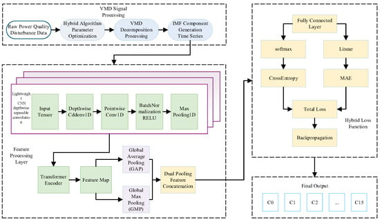
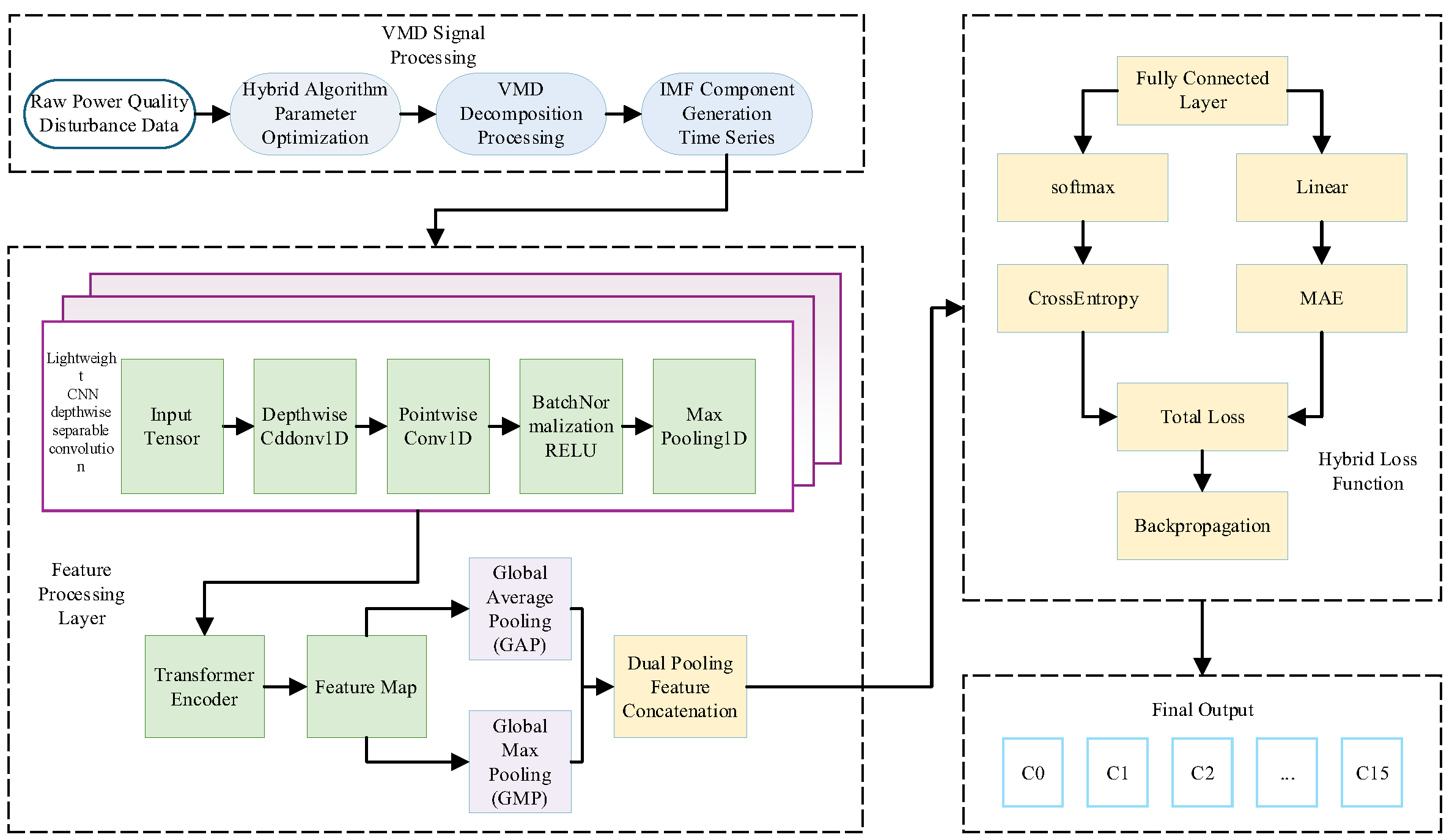
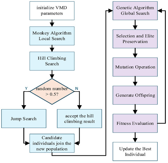
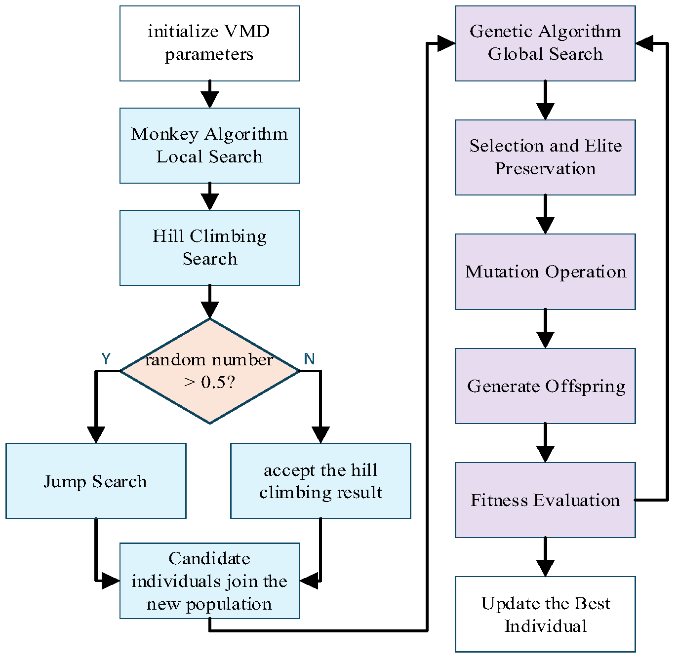
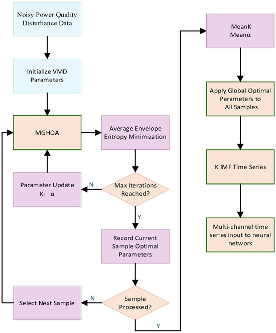
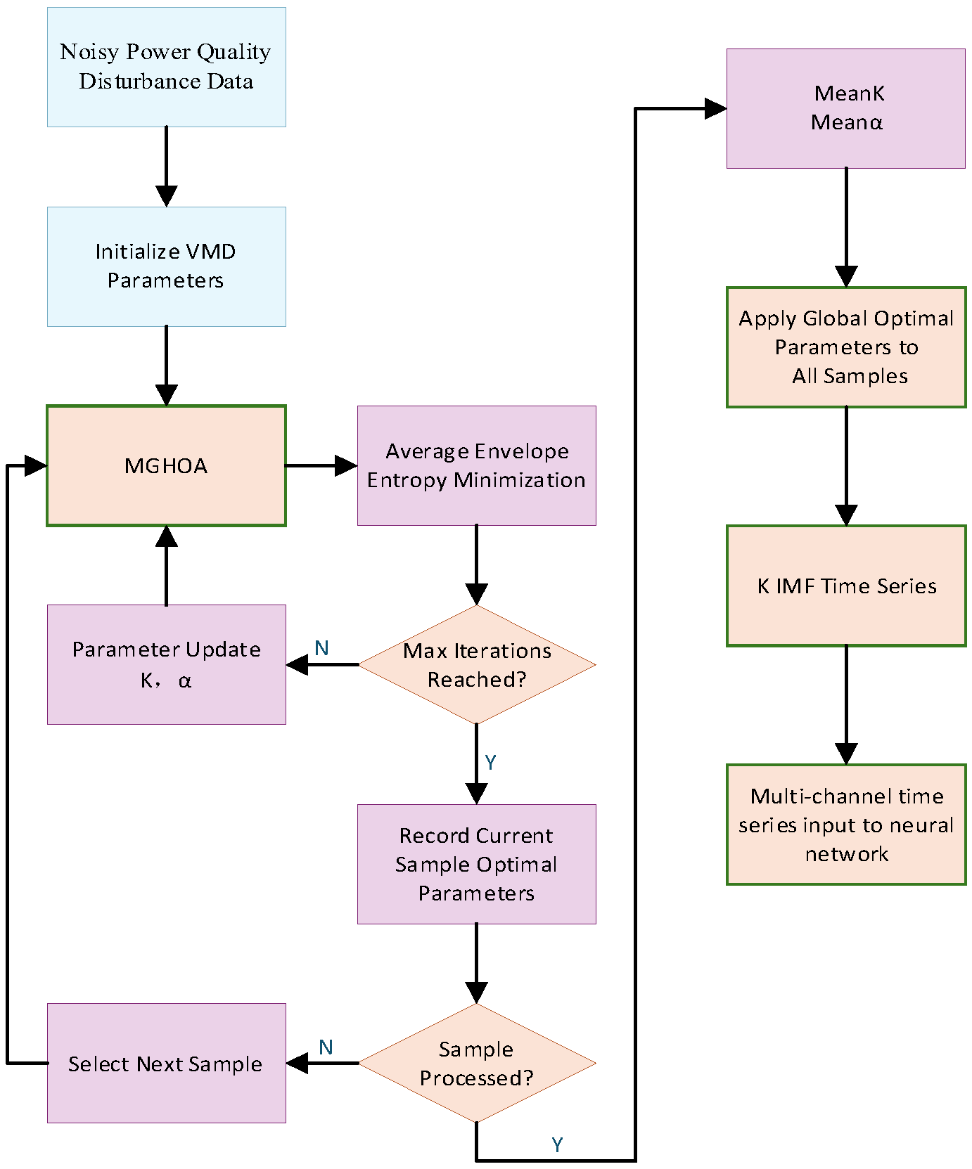
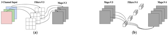
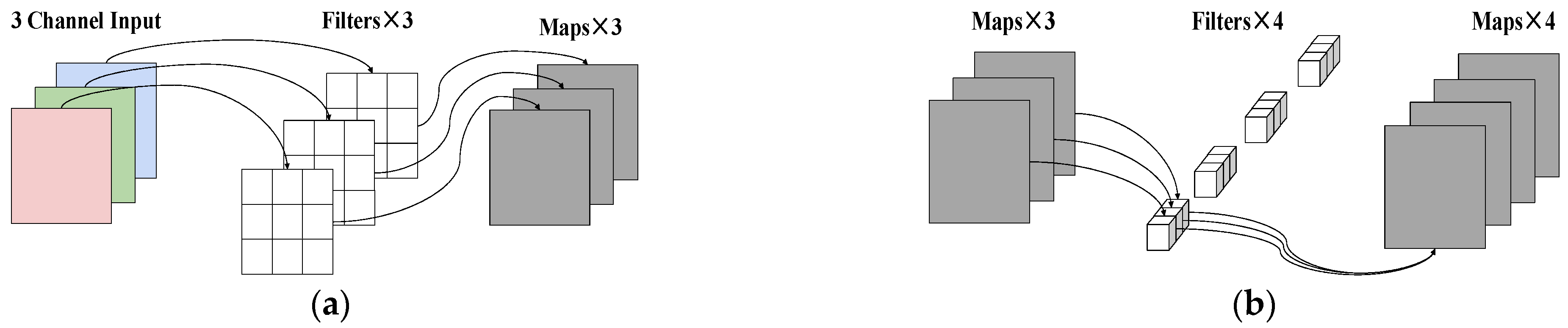
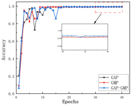
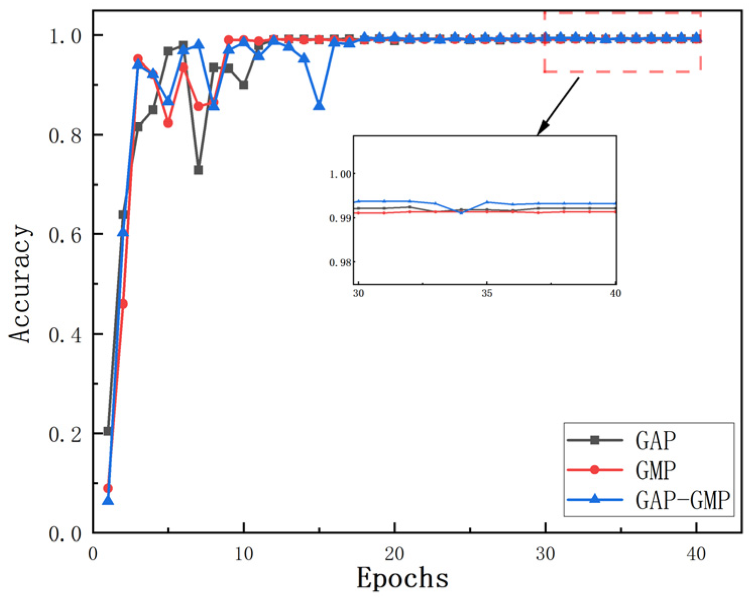
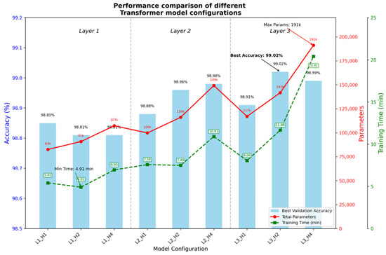
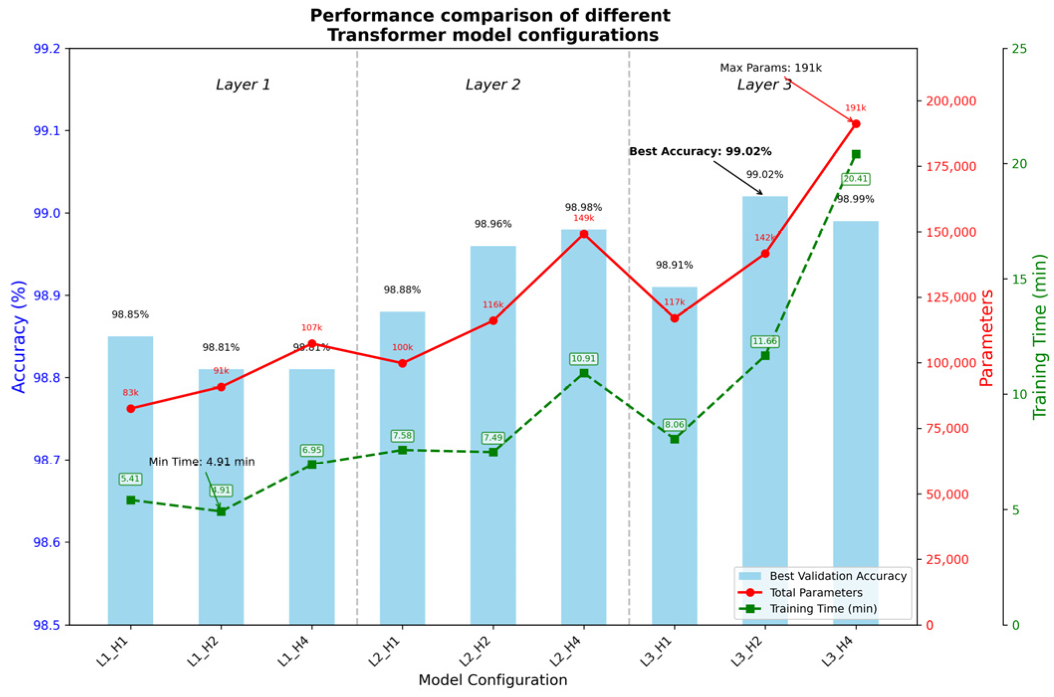
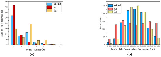
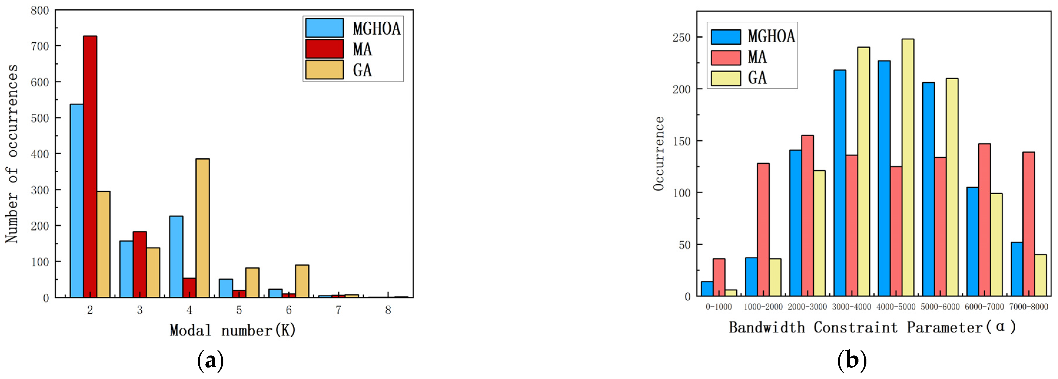
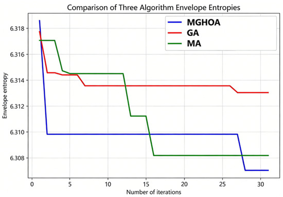
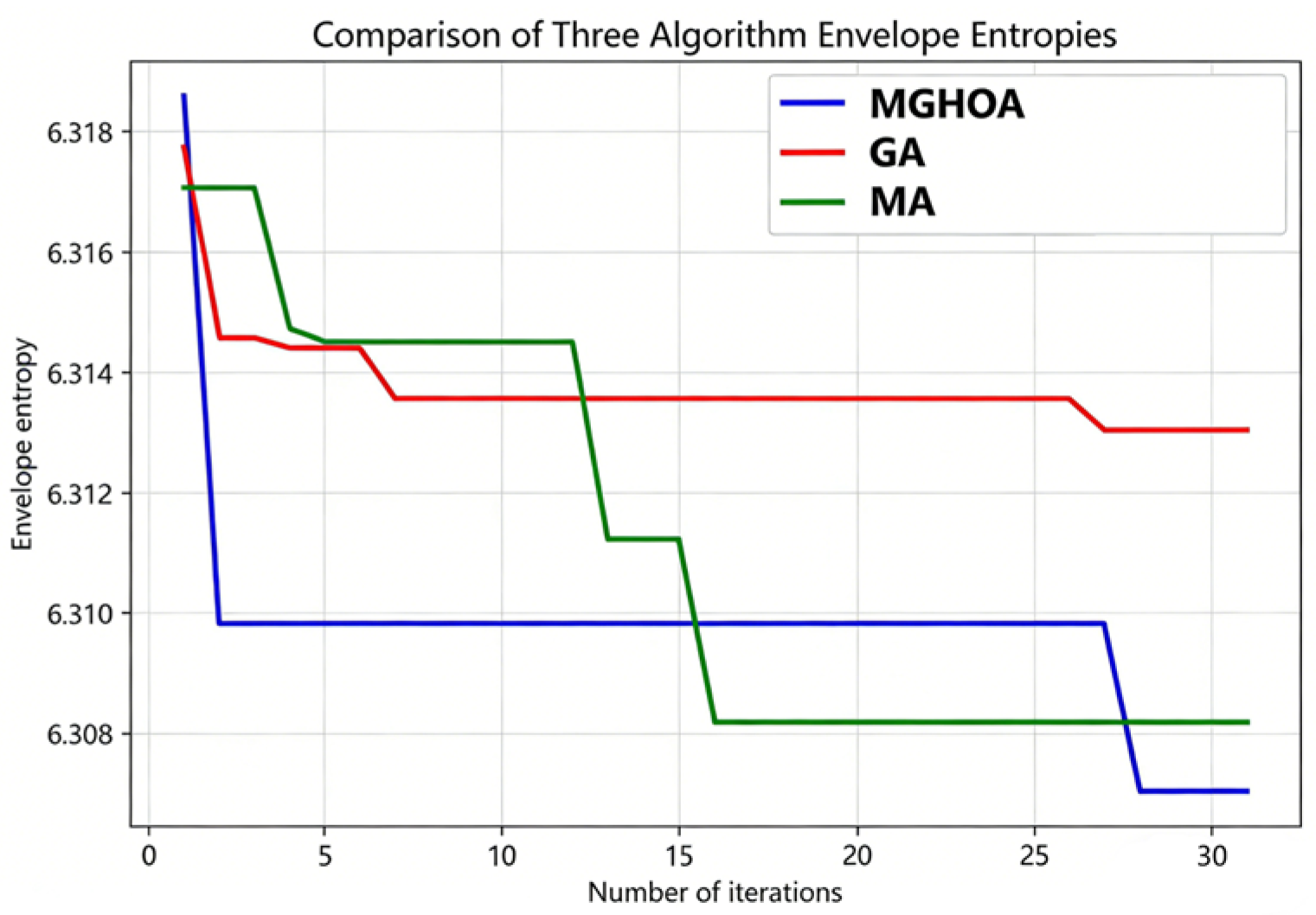
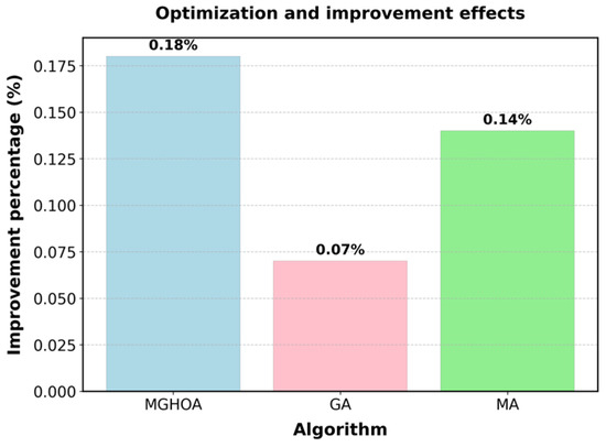
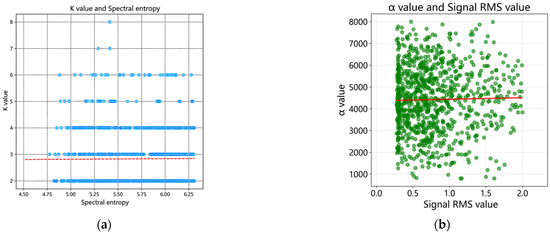
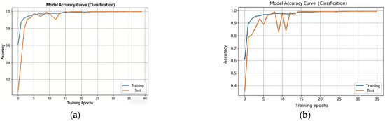
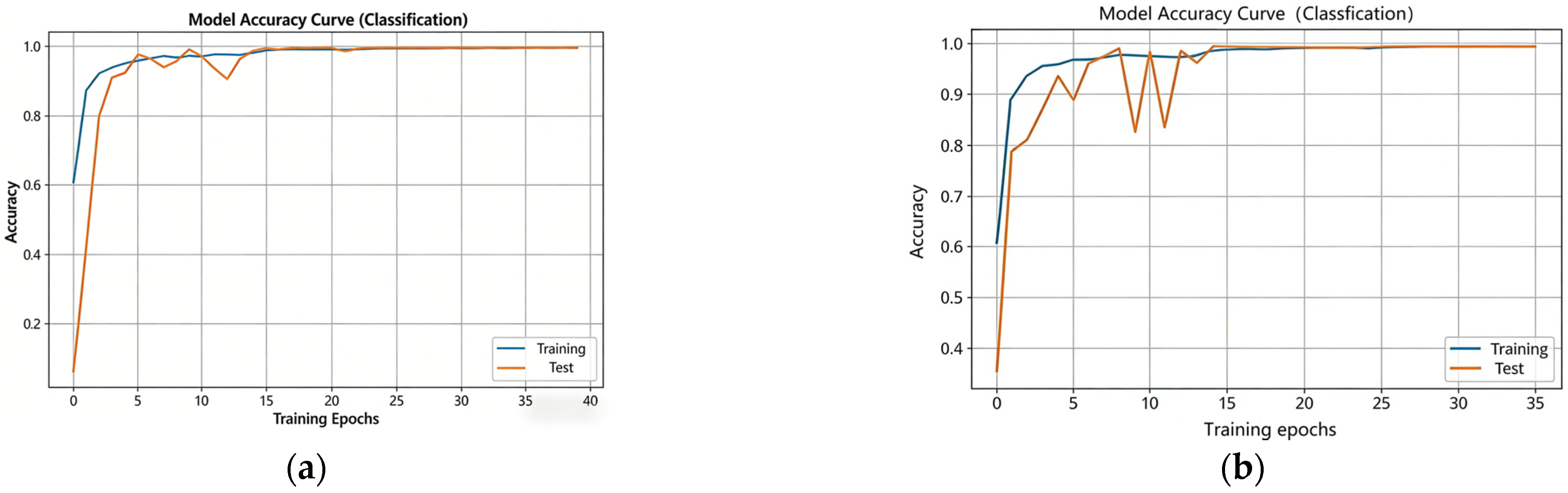
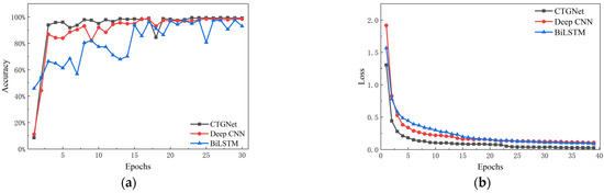
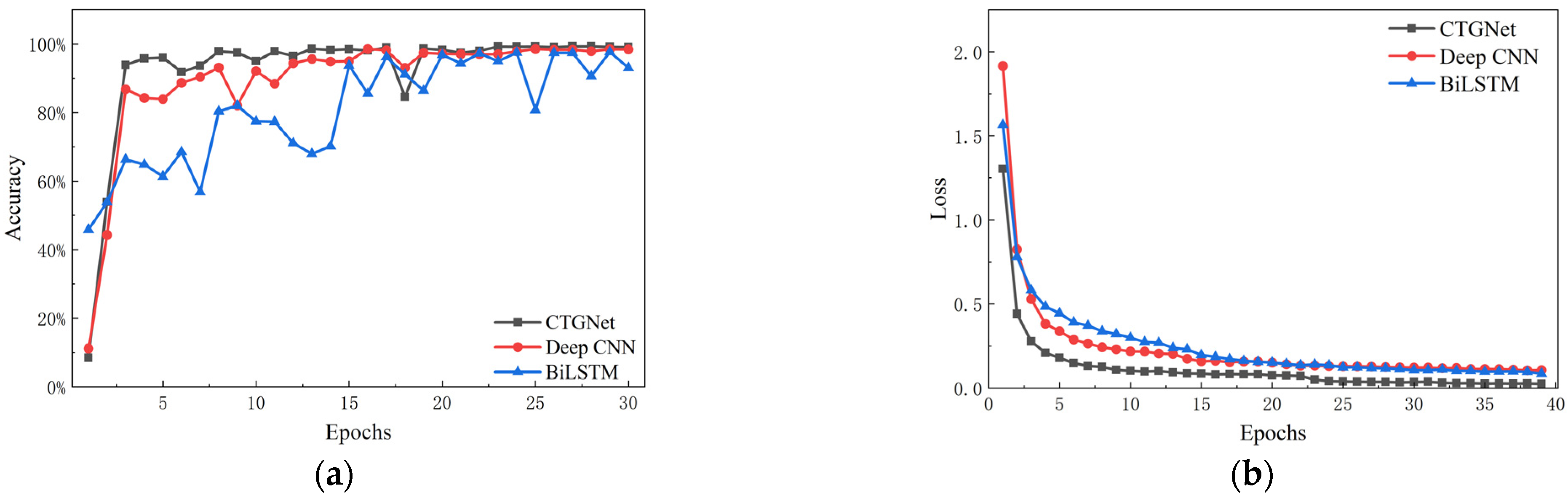

Disclaimer/Publisher’s Note: The statements, opinions and data contained in all publications are solely those of the individual author(s) and contributor(s) and not of MDPI and/or the editor(s). MDPI and/or the editor(s) disclaim responsibility for any injury to people or property resulting from any ideas, methods, instructions or products referred to in the content. |
© 2026 by the authors. Licensee MDPI, Basel, Switzerland. This article is an open access article distributed under the terms and conditions of the Creative Commons Attribution (CC BY) license.