


Abstract
In three-phase PWM rectifiers, abrupt load changes and parameter variations challenge DC-bus voltage regulation and degrade the performance of conventional controllers. To ensure robust regulation under nonlinear and time-varying conditions, this study proposes a type-3 fuzzy logic controller (T3-FLC) for DC-bus voltage regulation. The T3-FLC enhances the conventional type-1 framework by employing a three-dimensional membership structure that captures both vertical and horizontal uncertainties in the fuzzy inference process. This structure improves adaptability and stability in the face of system disturbances. The proposed controller was compared with a conventional proportional-integral (PI) controller and a type-1 fuzzy logic controller (T1-FLC) under different operating conditions: constant reference, reference tracking, load variation, regenerative operation, and grid disturbances. Under reference tracking mode, it settles within approximately 12 ms for the largest reference step, with the overshoot kept below 0.3%, whereas the T1-FLC and PI controllers require noticeably longer settling times and exhibit higher overshoot. In regenerative operation, the T3-FLC maintains tight DC-bus regulation with recovery times of 10–12 ms and an overshoot of about 2.7%, outperforming the benchmark controllers. Power quality analysis further shows that the proposed controller maintains low input-current distortion, with THD approximately 5–13%, and a near-unity power factor across all scenarios. These results confirm the T3-FLC as an effective control strategy for power converters.
1. Introduction
Conventional rectifiers, especially those based on diodes and thyristors, have been widely used in power electronics applications for many years. The basic advantages of these rectifiers include a simple structure, low cost, and high reliability. However, they have significant disadvantages, such as serious harmonic distortions in input current, low power factor (PF), and the inability to provide bidirectional power flow (BPF) [1,2,3]. Such structures have negative effects, especially on grid quality, and are insufficient in terms of harmonic current limitations and energy efficiency.
To overcome the limitations mentioned above, pulse-width modulation (PWM) rectifiers were developed, offering significant advantages over traditional rectifiers. PWM rectifiers have advantages, such as drawing sinusoidal current from the grid, maintaining input PF close to unity, and enabling regenerative operation by BPF. Furthermore, PWM rectifiers represent an attractive solution for industrial applications due to their low DC-bus voltage ripple and high dynamic performance [4,5].
The proportional-integral-derivative (PID) controller is a common choice for PWM rectifiers. Its appeal lies in its simple structure, easy implementation, and low computational cost [6,7]. Even so, when the system is nonlinear, as in PWM rectifiers with time-varying parameters and disturbances, fixed-gain PID often fails to maintain its performance across operating conditions. It works well when the system can be treated as fixed and linear, but in practice, rectifiers face parameter variations, inherent nonlinearities, and abrupt load transients. Under those conditions, PID can trigger instability, oscillations, and voltage overshoot. The issue becomes pronounced during reference-voltage changes: the controller should drive the system quickly and stably to the new operating point, yet classical PID often exhibits delayed response, long settling time, and weak disturbance rejection. The literature traces these shortcomings to limited adaptivity to changing dynamics and modest robustness to external disturbances [8].
Due to the limitations of fixed-gain PID controllers in nonlinear systems, various advanced control strategies have been investigated. The main alternatives are briefly reviewed below to position the proposed method. Within this framework, sliding-mode control provides strong robustness to modeling errors and disturbances, but it is susceptible to chattering unless higher-order or filtered designs are employed [9,10]. By contrast, backstepping offers a Lyapunov-based framework for regulating and the synchronous d–q frame currents. However, its recursive structure increases design complexity and parameter sensitivity [11,12]. Nonlinear MPC, in turn, delivers high multivariable performance at the expense of an online optimization burden that can hinder embedded real-time implementation [13,14]. Feedback linearization simplifies controller design by canceling nonlinear terms. However, it depends on an accurate model and can lose performance under parameter uncertainty [15,16,17,18]. Passivity-based control leverages energy shaping and damping injection, while practical deployment often hinges on constructing a suitable storage function [19,20]. Although nonlinear methods can improve control performance, their complex equations, high computational load, and stringent modeling requirements often limit their practicality. Accordingly, controllers with reduced model dependence that learn from system behavior and adapt to uncertainty have become increasingly desirable, motivating more flexible, learning-based, and adaptive control solutions.
In this direction, artificial intelligence-based control methods have emerged as a strong alternative for controlling nonlinear systems. Methods such as fuzzy logic, artificial neural networks, genetic algorithms, and fuzzy-neural systems reduce dependence on the system model and adapt more effectively to changing operating conditions [21,22,23]. These methods can create appropriate control laws by learning the behavior of the system based on experience. They offer effective results, especially in systems with model uncertainty or complex dynamic structures [24]. These methods have also been widely applied in the control of PWM rectifiers. Although type-1 fuzzy logic controllers (T1-FLCs) offer low computational cost with fixed membership functions (MFs), they may not provide sufficient performance in cases of high uncertainty. Type-1-based approaches have yielded successful results in controlling three-phase PWM rectifiers [25]. However, their performance is directly related to the definition of the rules and the sensitivity of the MFs. To overcome these limitations, type-2 fuzzy logic controllers (T2-FLCs) have been developed. Type-2 systems offer a more flexible and stable control structure by incorporating uncertainties into the model’s MFs [26]. However, the applications of these structures are more limited due to the high computational requirements [27]. While T1-FLCs only work with precise MFs [28], type-2 systems have a more flexible structure, especially in cases such as measurement noise and parameter uncertainty. However, these systems can only model second-order uncertainties [29]. Type-3 fuzzy logic controller (T3-FLC), on the other hand, provides a third-order uncertainty model on top of MFs, allowing more complex and multi-layered uncertainties to be managed [30,31].
Recent advances in T3-FLCs have followed two primary research directions: control applications and system optimization. In control applications, type-3 fuzzy sets demonstrate superior capability in handling third-order uncertainty, leading to consistent improvements in transient performance and robustness against parameter variations and external disturbances compared to conventional fuzzy controllers [32]. This is further supported by evidence showing that T3-FLC enhances transient metrics and strengthens maximum power point tracking stability under nonlinear regimes induced by operating condition variations, such as temperature and pressure [33]. Concurrently, in the field of optimization, significant progress has been made in developing practical implementation methods for type-3 fuzzy logic systems (T3-FLS). For hydrogen fuel-cell applications, interval type-3 PID designs have achieved notable improvements in tracking accuracy and disturbance rejection, leveraging the additional tuning flexibility inherent in type-3 modeling [34]. The integration of T3-FLS with optimization frameworks has yielded substantial benefits, including enhanced parameter tuning through harmony search algorithms [35] and enhanced search efficiency using interval type-3 adaptation in bee colony optimization [36]. Further advancing the field, a self-structuring approach based on invasive weed optimization has been developed to simultaneously optimize multiple parameters, including rule-base size, MF shapes, and secondary-membership parameters [37]. The foundations for the practical online adaptation of type-3 systems were established earlier through an online-learning interval type-3 control framework for power and energy management applications [38]. T3-FLCs can enhance dynamic performance, particularly due to their more robust structures against sudden changes [39]. With these features, they offer an effective solution by benefiting from both the simplicity of type-1 and the uncertainty management of type-2 [40].
Recent intelligent control strategies for three-phase PWM rectifiers have increasingly moved beyond conventional linear regulators. Early fuzzy-logic-based rectifier control demonstrated that three-phase PWM rectifiers can achieve satisfactory DC-bus voltage regulation and unity power-factor operation [25,41,42]. This direction was extended to neuro-fuzzy approaches, where nonlinear mapping capability was exploited to improve voltage regulation and synchronous-frame current control in PWM rectifiers [43]. More recent type-2 fuzzy neural network strategies have been reported to cope with uncertainty and parameter variations, including experimentally validated PD-type-2 fuzzy neural network control [44] and artificial-bee-colony-based type-2 fuzzy neural network control for DC-link voltage regulation under step changes, disturbances, unbalanced grid conditions, and regenerative operation [7]. Optimization-assisted interval type-2 fuzzy neural controllers have also shown improved transient behavior and robustness under different operating conditions [2]. In addition to fuzzy/neuro-fuzzy regulators, predictive and hybrid intelligent methods have been investigated for improved transient behavior and power quality (PQ) indices in PWM rectifiers [13,14,45]. Learning-oriented smart direct power control concepts have also been explored for ripple suppression and transient enhancement in three-phase PWM rectifiers [46]. Despite these developments, a systematic application of higher-order fuzzy uncertainty modeling, particularly type-3 fuzzy logic systems, to DC-bus voltage regulation in three-phase PWM rectifiers remains limited. This study aims to address this research gap through a systematic evaluation of the proposed T3-FLC for outer-loop DC-bus voltage regulation in a three-phase PWM rectifier and benchmarking it against PI and type-1 fuzzy logic baselines under a unified set of nominal, disturbed, and regenerative operating scenarios, clearly highlighting the novelty of the proposed approach.
In this study, a T3-FLC is designed and implemented in the outer control loop of a three-phase PWM rectifier. The control structure consists of two basic loops. The outer control loop aims to keep the DC output voltage of the system constant at the desired reference value, and the reference d-axis current obtained as the output of this loop is sent to the inner control loop. To ensure that the rectifier operates at a unity PF, the q-axis current reference is set to zero. The inner control loop performs high-bandwidth current control by monitoring the currents in the synchronous d–q frame separately in line with the obtained reference values. In both control loops, the structure is designed to be robust and to respond quickly to the system’s nonlinear dynamics. The developed T3-FLC provides both high accuracy output voltage regulation and high adaptability to system performance and disturbances.
For this evaluation, a detailed MATLAB/Simulink (R2023b, MathWorks, USA) model was developed to accurately represent the PWM rectifier’s control dynamics. The performance of the proposed controller was comprehensively evaluated under different operating scenarios: constant reference input performance, reference tracking, load disturbance rejection, regenerative operation, distorted grid voltage, grid voltage sag, grid voltage swell, and unbalanced grid. First, the operation at a constant reference DC-bus voltage was analyzed to examine the controller’s capability to maintain voltage regulation with minimal steady-state error and low ripple content. Second, the response to sudden changes in the reference DC-bus voltage was investigated, with emphasis on assessing overshoot and undershoot characteristics, as well as the settling time required for the system to reach its new equilibrium. Third, the system’s stability and regulation performance were tested under load variations on the DC side of the rectifier, allowing evaluation of its robustness to disturbances. The regenerative operating mode was simulated to analyze the system’s ability to reverse power flow, provide energy feedback to the grid, and preserve stability. Furthermore, the controller’s robustness was validated under four additional grid disturbances. The distorted grid voltage test evaluated harmonic immunity and its impact on total harmonic distortion (THD). The grid-voltage sag and swell scenarios assessed dynamic response, specifically the controller’s ability to maintain DC-bus voltage regulation during sudden voltage drops and to prevent over-voltage during voltage increases. Finally, the unbalanced grid test evaluated stability and ripple rejection performance under asymmetric conditions.
Based on these comprehensive simulation studies, the proposed T3-FLC exhibits superior performance in terms of both voltage regulation and system stability. Simulation results further confirm its robustness to uncertainties and sudden dynamic variations compared to T1-FLC and traditional PI controllers. The study’s results show that T3-FLCs are a promising alternative for PWM rectifier applications.
The main contributions of this study can be summarized as follows:
- To the best of the authors’ knowledge, this study is the first to systematically investigate a cascaded control scheme employing a type-3 fuzzy logic controller for the outer DC-bus loop, integrated with PI regulators for the inner synchronous d–q current loops.
- The T3-FLC improves transient performance in the examined scenarios, yielding shorter settling times and markedly lower overshoot than PI and T1-FLC in most operating conditions.
- Under dynamic operating scenarios, including sudden load transients and regenerative operation, the T3-FLC maintains tight DC-bus regulation with minimal overshoot/undershoot and exhibits strong disturbance-rejection capability.
- Across all investigated conditions, it maintains a near-unity PF and generally achieves competitive THD compared with the benchmark controllers, thereby enhancing PQ.
2. Three-Phase PWM Rectifier
The schematic representation of the three-phase PWM rectifier is shown in Figure 1. It consists of a three-phase AC source connected through line inductors and resistors to a voltage-source converter, where six IGBT switches (, , and ) operate under PWM control to regulate the DC-bus voltage . The DC side includes a smoothing capacitor C, and a resistive load [47]. The mathematical model is derived under the standard assumptions of balanced three-phase grid voltages, identical line impedances, and negligible switching and converter losses.
Figure 1.
Schematic of the three-phase PWM rectifier. The red dashed lines denote the PWM control signals, whereas the solid black arrows represent the direction of current flow.
The three-phase mathematical model of the rectifier on the AC side, derived from Kirchhoff’s Voltage Law, is presented in Equation (1) [48].
The three-phase AC grid voltages are given by Equation (2).
The input voltages of the three-phase rectifier are written as follows:
where denote the phase switching functions (or duty ratios). The power rectifiers employ a DC-bus capacitor to stabilize the voltage. The current through the capacitor located on the DC side is given by Equation (4).
Applying the Park transformation to Equation (5) yields the AC-side model of the rectifier in the synchronous d–q frame as in Equation (6). This representation facilitates the synthesis of current controllers, as follows [48,49]:
where and are the converter synchronous d–q frame voltages produced by the modulation signals . The DC-side dynamics are given by [48]:
For controller design, we introduce the decoupled virtual inputs as [48]:
which cancel the cross-coupling terms and feedforward the grid voltages. Substituting Equations (8) into Equation (6) yields the first-order current dynamics.
Equations (9) are consistent with the control algorithm in which the voltage commands are formed by adding feedforward and PI feedback to the decoupling terms [50].
3. Type-3 Fuzzy Logic Control
In this section, the fundamental concept and operating principles of the T3-FLC are introduced, covering its input–output structure, MF formulation, fuzzy rule base, and defuzzification process. Recently, T3-FLCs have emerged as an effective alternative for modeling and controlling highly uncertain and nonlinear systems [32,51]. While traditional T1-FLC and T2-FLC model uncertainty using crisp and interval-based MFs, respectively, T3-FLCs allow uncertainty to be represented with higher accuracy using three-dimensional MFs [52,53]. The overall fuzzy inference structure consists of conventional fuzzy operations: fuzzification, rule evaluation, aggregation, and defuzzification [54,55]. With type-3 MFs, both fuzzification and aggregation explicitly handle higher-dimensional uncertainty. The proposed controller is used for DC-bus voltage regulation of a three-phase PWM rectifier.
3.1. Overview of the T3-FLC Structure
Before presenting the mathematical formulation, this subsection provides an intuitive overview of the proposed T3-FLC. Figure 2 summarizes the main processing stages [56].
Figure 2.
Conceptual structure of the T3-FLC. Arrows indicate the sequential flow of signal processing from crisp inputs to final control action.
The controller operates on two crisp inputs: the DC-bus voltage error e and its change , as shown in the first block of Figure 2. These signals are first scaled or normalized by multiplying them with appropriate gains to map them to the required ranges for fuzzification. In the type-3 fuzzification stage, the scaled inputs are converted into type-3 fuzzy sets using three linguistic terms (Negative, Zero, Positive) for each variable. Unlike type-1 and type-2 fuzzifiers, the type-3 fuzzifier assigns a set of horizontally sliced membership surfaces to each term, representing different levels of uncertainty [30,52,53].
The membership evaluation stage computes the upper and lower membership degrees for each fuzzy set. These membership values drive the rule-activation block, where the if-then rules are triggered. Each rule expresses a qualitative control action (e.g., “if e is Positive and is Positive, then apply a strong corrective effort”). For each activated rule, the firing-strength computation block determines its strength, after which the aggregation block combines the firing strengths into a single fuzzy output. The type-reduction and defuzzification stage then collapses this high-dimensional type-3 output set into an interval type-2 set and converts it to a crisp value [30,32]. The resulting crisp control signal u is applied as the final control action and is used to generate the d-axis current reference in the outer control loop.
3.2. Type-3 Membership Function Formulation
This subsection details the MFs used in the fuzzifier block of Figure 2, specifying how the interval type-3 sets for e and are constructed. The structure of the proposed type-3 MFs for the input variables is shown in Figure 3, where the primary and secondary membership dimensions illustrate the third-order uncertainty modeling capability. Each input () is associated with a set of type-3 MFs whose centers are collected in (for brevity, the elements of and are not enumerated). For a generic linguistic term, a type-3 MF is represented by upper and lower membership surfaces parameterized by a horizontal slicing parameter . Intuitively, the upper and lower surfaces capture the uncertainty bounds of the membership grade for the same rule slice, while the horizontal slice level controls how the membership surface decays across the operating domain. Let denote the MF center, and , the left and right spreads, respectively. Here, and determine the support/width of each MF on the left and right sides around the center (i.e., where the membership becomes zero). The upper surfaces are given by [52,53]
and the lower surfaces are
where x is the scalar input (with centers collected in or ), is the MF center, and are the left/right spreads, and are upper/lower shape (slice) exponents for horizontal slice j.
Figure 3.
Type-3 MF representation for the T3-FLC inputs. The magenta curves denote the secondary MFs, while the green shaded regions represent the primary MFs; black lines indicate their boundaries.
With this definition, the membership grade reaches 1 at the center () and becomes 0 outside the support interval set by the spreads. Moreover, the slice exponents and shape the curvature/steepness of the upper and lower surfaces, respectively, thereby controlling how rapidly the membership decreases as the input moves away from the MF center.
As illustrated in Figure 3, for each input variable of the T3-FLC, only three MFs (L, Z, and R) are employed. The L/Z/R partitions provide a compact linguistic cover for negative, near-zero, and positive operating regions of the input, while the uncertainty is represented through the additional upper/lower bounds and the slice exponents . Although this number is smaller than the five- or seven-term partitions commonly used in T1-FLCs, each type-3 MF contains four independent bounds, providing a richer representation of uncertainty. Therefore, three linguistic terms are sufficient to cover the full operating range while keeping the rule base compact.
In practice, mainly determines how wide each linguistic region remains active, whereas mainly governs how sharp the membership drop is for each horizontal slice, which together support good coverage with a small rule set. This structure reduces the online computational burden and avoids generating a large number of low-firing or inactive rules, thereby improving real-time feasibility without sacrificing control accuracy or dynamic performance [52].
The nonlinear input–output mapping realized by the proposed T3-FLC is illustrated in Figure 4. The surface shows how the controller maps the DC-bus voltage error e and its change to the normalized control output u. For a wide range of negative and positive errors, the surface remains relatively smooth and bounded, indicating that the T3-FLC avoids excessively aggressive control actions while still providing sufficient corrective effort. The repeating dome-shaped patterns reflect the activation of different rule combinations as move across the operating space, allowing the controller to modulate its response to both the magnitude and the rate of change of the voltage deviation.
Figure 4.
Rule surface of the implemented T3-FLC mapping the DC-bus voltage error e and its change to the control output u.
3.3. Fuzzy Rule Base and Firing Strength Computation
This subsection formalizes the rule-base and firing-strength computation stages depicted in Figure 2, focusing on the structure of the former and the derivation of firing strengths for each type-3 rule. The rule base maps linguistic terms from input 1 (with centers denoted by ) and input 2 (with centers denoted by ) to a specific set of singleton consequents. A generic rule is given by [52,53]:
For a given horizontal slice level , the product t-norm is used to compute the four firing strengths (upper–upper, lower–lower, upper–lower, and lower–upper):
where indexes the fuzzy rules; R is the total number of rules. The four firing strengths correspond to upper–upper, lower–lower, upper–lower, and lower–upper slice combinations obtained by product t-norm.
3.4. Output Computation and Defuzzification
Once the firing strengths are determined, the aggregation stage—as depicted in Figure 2—combines them into partial outputs. For the upper and lower sides at slice , these are obtained by taking normalized weighted sums of the singleton consequents as follows [52,53]:
where and are the aggregated upper/lower singleton consequents of rule l (in implementation, collects , and collects ). If needed, a small regularizer can be added to denominators to avoid division by zero. The crisp output of T3-FLC is computed as a convex combination of the slice endpoints as follows [52,53]:
where K is the number of horizontal slices; , are nonnegative slice weights, and , are the lower/upper partial outputs at slice j. In our implementation, , so reduces to the average of the two endpoints. A single slice is adopted to minimise the online computational burden whilst preserving the essential upper–lower uncertainty structure of the type-3 output.
4. The Proposed Control Method
The proposed cascaded control scheme, illustrated in Figure 5, consists of a T3-FLC-based DC-bus voltage controller (outer control loop) and inner current control loops in the synchronous frame. The architecture cleanly separates slow DC-bus energy regulation (outer control loop) from fast current dynamics (inner synchronous d–q frame loops), enabling loop-by-loop tuning and robust execution of the commanded converter voltages that are finally mapped to sinusoidal PWM.
Figure 5.
Proposed cascaded control architecture: T3-FLC for DC-bus voltage regulation and inner PI-controlled d–q current loops with decoupling. Note: Asterisks on variables denote reference signals.
Phase voltages and line currents are measured. A phase-locked loop (PLL) estimates the grid phase angle ; the currents are then mapped to the synchronous d–q frame via the Clarke–Park transformations, as expressed in the following equation.
where and are the currents on the d- and q-axes, while and represent the Clarke and Park transformation operators, respectively. The d-axis is aligned with the grid voltage; therefore, and represent the frame components synchronous d–q of the grid voltage.
4.1. Outer Control Loop: DC-Bus Voltage Regulation with a T3-FLC
The outer control loop regulates the DC-bus voltage around its reference . In continuous time, the voltage error and its time derivative are defined as
The T3-FLC receives two normalized inputs derived from the scaled forms of these quantities:
where are input scaling factors. In the digital implementation with sampling period , the error and its rate of change are computed as
and the normalized inputs of the T3-FLC become
These two input variables are converted into fuzzy sets through a fuzzification process using the predefined type-3 MFs. The fuzzified inputs are processed by the T3-FLC rule base, and the inference mechanism produces a fuzzy output, which is then defuzzified into a crisp control signal. The T3-FLC output represents the rate of change of the d-axis current reference:
and the integrator block yields
where is the output scaling factor. In this study, the scaling factors , , and were all set to unity (), so that the voltage error e, its derivative , and the defuzzified output are used directly without additional scaling. Tuning was performed by adjusting the type-3 MF parameters—the centers , the left and right spreads and , and the slice exponents and —rather than the input or output gains, thus keeping the controller structure simple and focusing the design effort on the fuzzy sets that define the nonlinear mapping. The MF parameters were tuned manually through iterative trial-and-error simulations, guided by performance metrics such as DC-bus voltage overshoot, settling time, and steady-state ripple. Initial values for the spreads and slice exponents were chosen from ranges commonly used in type-3 fuzzy control; fine-tuning was conducted over several simulation runs until the closed-loop response met acceptable specifications. The chosen parameters were validated by comparing T3-FLC performance with PI and T1-FLC under the same test conditions (Section 5), confirming that the manually tuned configuration yields competitive or superior regulation.
To prevent over-current and integrator windup, a saturation mechanism ensures . To keep the PF close to unity, the current reference of the q-axis is set to . In discrete time, the reference is updated as
Thus, the T3-FLC directly shapes the evolution of the current reference on the d-axis, linking the fuzzy decision-making process to the physical current control loop.
4.2. Inner Control Loops: d–q Current Control and Decoupling
The synchronous-frame currents are regulated by PI controllers augmented with cross-coupling feedforward based on the line inductance and the grid angular frequency (from the PLL); the line resistance may be neglected if sufficiently small. The resulting synchronous d–q frame voltage commands are
where and are the d- and q-axis voltage commands of the converter, and are the PI gains of the inner current loops. The terms and in Equation (29) provide the standard decoupling. The and are mapped back to the frame through the inverse Park transformation and then applied to a sinusoidal PWM, thereby generating the gate pulses for the three phase PWM rectifier.
5. Results and Discussion
In this section, the performance of the proposed three-phase PWM rectifier system integrated with the T3-FLC is evaluated and compared with conventional PI and T1-FLC controllers. Both steady-state and transient behaviors are analyzed under multiple operating conditions using a common set of time-domain and PQ indices. The simulation framework, control architecture, and case-study results are detailed in the following subsections.
5.1. Simulation Framework and Control Architecture
To comprehensively evaluate the performance of the proposed three-phase PWM rectifier system controlled by the T3-FLC, four operating scenarios were simulated in MATLAB/Simulink: constant reference, reference tracking, load disturbance, and regenerative operation. PQ performance was also evaluated under harmonic injection, sag/swell, and voltage unbalance. The overall structure of the three-phase PWM rectifier system and its T3-FLC-based control sub-blocks are illustrated in Figures S1–S3, and all simulations were conducted with the system and controller settings summarized in Table 1. The detailed Simulink schematics of the model and its sub-blocks are provided in the Supplementary Material.
Table 1.
System and controller parameters used in the study.
The DC-bus voltage responses of all controllers are comparatively illustrated, while detailed waveforms, such as the synchronous d–q frame currents, grid voltage–current profiles, and active–reactive power trajectories, are provided specifically for the T3-FLC to highlight its control dynamics. Furthermore, Section 5.3 presents PQ analysis, including input-current THD, PF, and efficiency evaluations, performed for both the main operating conditions and additional grid disturbances such as harmonic injection, voltage sag/swell, and voltage unbalance events.
Performance Metrics and Evaluation Methodology
To ensure a consistent and meaningful comparison of the PI, T1-FLC, and T3-FLC, a unified set of time-domain and PQ metrics are used for all operating conditions, including reference tracking, load disturbances, regenerative operation, and grid-side disturbances (harmonic injection, voltage sag/swell, and unbalance). The time-domain indicators primarily describe the DC-bus voltage response, whereas the PQ metrics characterize the quality of the grid currents and the overall energy conversion. The performance metrics used to evaluate the T3-FLC-based DC-bus voltage controlled rectifier are summarized below.
- Rise/fall time (, ): the time required for the DC-bus voltage to traverse from 10% to 90% of the step change. For a step-up (reference increase), is measured; for a step-down (reference decrease), is measured.
- Settling time (): the time required for the DC-bus voltage to enter and remain within a band around its final steady-state value after a disturbance or reference change.
- Recovery time (): the time required for the DC-bus voltage to return to and remain within a band around its steady-state (or reference) value after a disturbance.
- Overshoot/undershoot (, %): the maximum positive (overshoot) and negative (undershoot) deviation of the DC-bus voltage with respect to its reference value during the transient interval, normalized to the reference voltage.
- DC-bus voltage ripple (, %): the peak-to-peak variation of the DC-bus voltage in steady state, normalized to its steady-state value.
- Steady-state efficiency (, %): the ratio of the average output active power on the DC side to the average input active power drawn from the grid under steady-state conditions.
- Steady-state power factor (): the ratio of the steady-state active power to apparent power at the grid side.
- Grid current THD (, %): the THD of the grid current in steady state, defined as the ratio of the rms value of all harmonic components to the rms value of the fundamental component, obtained from the FFT of the phase current.
By consistently applying this common set of indices across all simulations, a comprehensive comparison of the PI, T1-FLC, and T3-FLC controllers is achieved in terms of transient speed, robustness, voltage regulation, and overall PQ performance.
5.2. Dynamic Performance and Robustness Comparison
This subsection compares the dynamic performance and robustness of PI, T1-FLC, and T3-FLC under four operating conditions.
5.2.1. Response Under Constant Reference Input
This case study investigates the controllers’ performance under a constant DC-bus reference of 200 V to evaluate their transient response, steady-state regulation, and overall dynamic performance. The primary objective is to verify the effectiveness of the proposed T3-FLC in maintaining a smooth and accurate DC voltage regulation compared to conventional benchmarks.
The simulation results for Case Study 1 are presented in Figure 6. Figure 6a illustrates the comparative DC-bus voltage responses of the PI, T1-FLC, and T3-FLC controllers, while Figure 6b–e show the d-axis current, q-axis current, grid voltage–current waveforms, and active–reactive power characteristics obtained specifically for the T3-FLC. The corresponding quantitative performance metrics are summarized in Table 2.
Figure 6.
Simulation results under constant 200 V DC-bus reference (Case Study 1): (a) DC-bus voltage, (b) d-axis current, (c) q-axis current, (d) phase a voltage and current, (e) active and reactive power. Note: The cyan dashed box indicates the zoomed transient region.
Table 2.
Dynamic and steady-state performance metrics of controllers for Case Study 1.
A comparative evaluation of the rise time shows that the PI controller yields the fastest initial response of 7.65 ms, followed by the T3-FLC with 9.65 ms, while the T1-FLC exhibits the slowest response of 12.05 ms. Although the PI rise time is approximately 21% shorter than that of the T3-FLC, this marginal advantage is outweighed by its considerably longer settling time and excessive overshoot. In terms of settling time, the T3-FLC outperforms the other controllers, stabilizing the system within 15.65 ms, which is about 4.8 times faster than the PI controller with 74.85 ms and also notably faster than the T1-FLC with 22.45 ms. The overshoot analysis further highlights the effectiveness of T3-FLC, which limits the overshoot to only 0.18%, compared to 0.30% for the T1-FLC and a significantly higher 13.58% for the PI controller. The PF values remain close to unity for all controllers because the q-axis current reference was set to zero and the d–q current decoupling structure preserves reactive-power compensation. Therefore, the observed differences mainly appear in the THDi. This metric is determined by how accurately the inner current loops track during each controller’s transient correction. Overall, these results indicate that the T3-FLC provides the most balanced transient performance, combining negligible overshoot with robust DC-bus voltage regulation.
5.2.2. Reference Tracking Response
This case evaluates the controller’s ability to track changes in the reference signal in terms of response speed, overshoot, and steady-state accuracy. Simulation results for Case Study 2 are depicted in Figure 7. Figure 7a compares the DC-bus voltage responses of PI, T1-FLC, and T3-FLC. Figure 7b–e present the d-axis current, q-axis current, grid voltage–current waveforms, and active–reactive power characteristics for T3-FLC. In this operating condition, the DC-bus reference voltage is varied stepwise: maintained at 200 V between 0–0.2 s, increased to 250 V between 0.2–0.4 s, and subsequently restored to 200 V between 0.4–0.6 s. The 250 V reference level, corresponding to a 25% increase, was selected to provide a moderate yet sufficiently challenging voltage step for evaluating the controllers’ transient tracking capability. This test setup provides a basis for evaluating the transient response characteristics of the controllers under reference variations. The corresponding quantitative performance indicators for Case Study 2 are summarized in Table 3.
Figure 7.
Simulation results under step reference changes (200 V → 250 V → 200 V, Case Study 2): (a) DC-bus voltage, (b) d-axis current, (c) q-axis current, (d) phase a voltage and current, (e) active and reactive power. Note: The cyan and pink dashed boxes indicate the zoomed transient regions.
Table 3.
Performance metrics of controllers in different time intervals for Case Study 2.
With respect to rise/fall time, the T3-FLC exhibits the fastest transient response in both intervals, with rise/fall times of 9.05 ms in the 250 V step-up interval and 6.00 ms in the 200 V step-down interval. The PI controller exhibits the slowest dynamics, with rise/fall times of 18.55 ms and 18.00 ms, respectively. The T1-FLC yields intermediate responses of 11.80 ms and 14.00 ms across the tested intervals. Regarding settling time, the T3-FLC outperforms the other controllers, achieving steady-state operation within 11.50 ms in the step-up interval and 7.70 ms in the step-down interval. This is substantially faster than the PI controller, which requires 62.95 ms and 63.05 ms, and also superior to the T1-FLC, with settling times of 15.60 ms and 18.95 ms. These results underline the superior consistency and transient performance of the T3-FLC in handling reference changes. A comparative assessment of overshoot further substantiates these findings. In the step-up interval, T3-FLC limits overshoot to 0.256%, compared with 0.312% (T1-FLC) and 2.608% (PI). In the step-down interval, T3-FLC limits undershoot to 1.088%, which is lower than 1.151% (T1-FLC) and 3.609% (PI). In the reference-tracking case, the observed differences in THDi across controllers stem from the coupling between the outer-loop voltage regulation and the inner d–q current tracking. The PI controller can provide slightly better harmonic cancellation in some intervals due to its fixed-gain behavior near steady operation, while T3-FLC prioritizes faster and more well-damped outer-loop corrections, resulting in a different transient modulation pattern. Collectively, the T3-FLC provides the most balanced transient performance, combining rapid settling times and minimal overshoot in the step-up response with a moderate and well-damped undershoot in the step-down response.
5.2.3. Disturbance Rejection Under Load Variations
This test evaluates the controllers’ robustness by subjecting them to sudden load changes, measuring their ability to maintain voltage stability and recover quickly with minimal deviation. The simulation results for Case Study 3 are presented in Figure 8. Figure 8a provides a comparative overview of the DC-bus voltage response under load disturbances for the three controllers (PI, T1-FLC, and T3-FLC), while Figure 8b–e illustrate the d-axis current, q-axis current, grid voltage–current waveforms, and active–reactive power characteristics specifically for the T3-FLC. In this case, the load resistance is reduced from 40 to 20 at 0.2 s and subsequently restored to 40 at 0.4 s, allowing assessment of each controller’s disturbance rejection capability. The 40 nominal load was selected to represent the rectifier’s rated operating condition, ensuring realistic current and power levels within the converter’s safe limits, while the 20 step introduces a 100% load increase to test the controller’s robustness. The corresponding quantitative performance metrics are summarized in Table 4.
Figure 8.
Simulation results under load variation (40 → 20 → 40 , Case Study 3): (a) DC-bus voltage, (b) d-axis current, (c) q-axis current, (d) phase a voltage and current, (e) active and reactive power.
Table 4.
Performance metrics of controllers in different time intervals for Case Study 3.
As summarized in Table 4, this load disturbance scenario highlights the dynamic advantages of the T3-FLC. During the 0.2–0.4 s interval, the T3-FLC achieves the shortest recovery time of 7.35 ms, followed by the T1-FLC with 11.25 ms, whereas the PI controller requires 71.95 ms to restore the DC-bus voltage. In the subsequent 0.4–0.6 s interval, the same trend is preserved: the T3-FLC recovers within 7.15 ms, the T1-FLC within 11.45 ms, while the PI controller again exhibits a significantly slower response with a recovery time of 63.80 ms. The amplitude of the DC-bus deviation is also better controlled by the T3-FLC. For the load step-up interval, the T3-FLC limits the overshoot to 0.18%, compared to 0.301% for the T1-FLC and 0.266% for the PI controller.
Following the load reduction at 0.4 s, the T3-FLC achieves the smallest undershoot of 0.113%, while the T1-FLC and PI controllers exhibit undershoots of 0.155% and 0.324%, respectively. In terms of steady-state DC-bus ripple, the T3-FLC reduces to 0.348% in the 20 interval and 0.280% in the 40 interval. This consistently improves upon the PI controller, which shows ripples of 0.485% and 0.431%. The T1-FLC provides slightly lower ripple than the T3-FLC after the load decrease, with 0.252%, but at the cost of slower recovery. Regarding PQ, all controllers maintain nearly unity PF, with PFss equal to 0.998 at 20 and 0.992 at 40 , and a very similar efficiency of 99%. The PI controller achieves the lowest current THD during the heavy-load interval, with THDi equal to 4.613%, while the T3-FLC yields 5.702% and the T1-FLC 6.084%. However, after the load returns to 40 , the T3-FLC provides the lowest distortion, with a THDi of 10.803%, slightly outperforming both the PI and T1-FLC controllers. During load transients, the transient modulation from the outer-loop controller affects the instantaneous current waveform and, in turn, the measured THDi. The PI controller can yield lower THDi in specific intervals where d-axis tracking remains close to a linear steady operating point, whereas T3-FLC achieves markedly faster recovery and better voltage damping. This yields competitive (but sometimes slightly higher) THD due to the distinct transient current-shaping induced by the fuzzy control effort. These results indicate that the T3-FLC offers a favorable compromise, achieving competitive PQ alongside very fast recovery and well-damped DC-bus deviations under abrupt load variations.
5.2.4. Performance in Regenerative Operation
This case examines controller stability during BPF, testing their ability to handle the reverse energy transfer from the DC side to the grid while maintaining voltage regulation. Simulation results for Case Study 4 are illustrated in Figure 9. Figure 9a shows the comparative DC-bus voltage response under regenerative operation for the three controllers (PI, T1-FLC, and T3-FLC). Figure 9b–e present the d-axis current, q-axis current, grid voltage–current waveforms, and active–reactive power characteristics corresponding to the T3-FLC. In this scenario, a 250 V DC source with an internal resistance of 3 is connected to the DC side at 0.2 s and disconnected at 0.4 s, triggering regenerative events. The DC source voltage is set approximately 25% higher than the nominal 200 V DC-bus reference to intentionally trigger a controlled regenerative event while maintaining system stability. This voltage difference should ensure sufficient potential for reverse energy transfer without exceeding the converter’s safe operating limits. The corresponding quantitative performance indicators are summarized in Table 5.
Figure 9.
Simulation results under regenerative operation (250 V DC source connected at 0.2–0.4 s, Case Study 4): (a) DC-bus voltage, (b) d-axis current, (c) q-axis current, (d) phase a voltage and current, (e) active and reactive power showing BPF.
Table 5.
Performance metrics of controllers in different time intervals for Case Study 4.
All controllers successfully maintain stable operation under regenerative conditions. However, there are clear differences in the recovery, overshoot, and undershoot behavior. During the first regenerative interval from 0.2 s to 0.4 s, the T3-FLC achieves the fastest recovery, with a recovery time of 11.40 ms, followed by the T1-FLC with 18.90 ms. The PI controller requires 148.65 ms to re-establish steady-state operation. In the subsequent interval from 0.4 s to 0.6 s, the same trend holds: the T3-FLC recovers within 10.60 ms and the T1-FLC within 14.45 ms, while the PI controller again exhibits a much slower response with a recovery time of 102.65 ms. The amplitude of the DC-bus deviation is also significantly better controlled by the fuzzy controllers. In the first interval, the T3-FLC limits the overshoot to 2.675%, while the T1-FLC and PI controllers reach 4.244% and 11.073%, respectively. After the DC source is disconnected at 0.4 s, the undershoot becomes the dominant transient. In this interval, the T3-FLC confines the undershoot to 3.128%, compared with 4.819% for the T1-FLC and 17.71% for the PI controller. In terms of steady-state DC-bus ripple, the T1-FLC provides the lowest , with 0.301% in the first interval and 0.186% in the second. The T3-FLC achieves slightly higher but still low values of 0.374% and 0.238%, respectively. The PI controller, by contrast, exhibits substantially larger ripples of 1.576% and 0.670%.
In the first interval, all controllers maintain an almost unity negative PF of , indicating that the grid current is nearly out of phase with the grid voltage. This behavior is illustrated in Figure 9e. In the second interval, PF is close to 0.992 across all controllers. The efficiencies are close to each other, 98.3–98.9%. The PI controller attains the lowest THDi during the first regenerative interval, with THDi equal to 4.068%, while the T3-FLC and T1-FLC yield 4.655% and 5.771%. In the second interval, the T3-FLC provides the lowest distortion, with a THDi of 10.80%, slightly improving the PI and T1-FLC controllers. In regenerative operation, PF remains close to the expected values (including negative power factor when power flows back) due to the maintained current reference structure in the d–q frame. The remaining controller-dependent differences in THDi are primarily linked to how quickly and smoothly the controllers re-establish after power-flow reversal, which shapes the harmonic content of the grid current. In brief, these results show that under regenerative operating conditions, the T3-FLC offers the most favorable compromise, combining very fast recovery and well-damped DC-bus deviations with competitive PQ performance.
Figure 10 summarizes the comparative performance of the PI, T1-FLC, and T3-FLC controllers over the four main simulation cases. Each subplot corresponds to one metric: (a) maximum overshoot, (b) settling/recovery time, (c) DC-bus voltage ripple, and (d) input current THD. Case Study 1 shows steady-state results at a fixed reference; Case Studies 2–4 show two intervals per case, with different hatching used to separate the two time windows (e.g., 0.2–0.4 s and 0.4–0.6 s). In general, the T3-FLC shows lower overshoot, shorter settling/recovery times, and reduced voltage ripple compared to PI and T1-FLC, while maintaining competitive THD levels.
Figure 10.
Performance comparison of PI, T1-FLC, and T3-FLC controllers across four case studies: (a) Maximum overshoot (, %), (b) Settling/recovery time (, ms), (c) DC bus voltage ripple (, %), (d) Current total harmonic distortion (THDi, %). For Case 2–4, results are shown for both intervals (0.2–0.4 s and 0.4–0.6 s) with different hatching patterns (diagonal and cross-hatching). Case 1 represents steady-state performance with a single interval.
5.3. Power Quality Analysis
A thorough assessment of PQ is essential for evaluating the effectiveness and robustness of PWM rectifier control strategies, particularly under distorted or dynamic operating conditions. In this study, PQ performance is examined through key indicators such as the THDi, the PFss, and the . These metrics collectively capture the controller’s ability to ensure sinusoidal grid current injection, maintain efficient power transfer, and regulate the DC-bus voltage with minimal ripple.
The analysis encompasses both nominal operation and various grid disturbance scenarios, including harmonic injection, voltage sag, voltage swell, and voltage unbalance. By systematically comparing the PI, T1-FLC, and T3-FLC controllers across these conditions, this section highlights the strengths and limitations of each control strategy from a PQ perspective.
5.3.1. Harmonic Distortion Case
This case is used to evaluate the controller’s performance under distorted grid conditions caused by injected voltage harmonics, focusing on DC-bus voltage regulation, current THD, and PF. In the harmonic distortion scenario, where 5% 5th- and 5% 7th-order voltage harmonics are injected into the grid, all three controllers are able to maintain acceptable steady-state performance, but with distinct trade-offs, as summarized in Table 6. The corresponding DC-bus voltage, AC grid voltage/current waveforms, and their harmonic spectra are illustrated in Figure 11a–d. In terms of DC-bus voltage ripple, the fuzzy controllers clearly outperform the PI controller: the T1-FLC achieves the lowest with 0.269%, followed by the T3-FLC with 0.309%, whereas the PI controller exhibits a significantly higher ripple of 0.510%. Conversely, the PI controller provides the lowest input-current distortion, with THDi equal to 10.543%, while the T1-FLC and T3-FLC yield slightly higher values of 11.009% and 11.504%, respectively. Despite these differences, all controllers maintain the same steady-state PF of 0.992 under harmonic injection, indicating that the displacement and distortion effects are well controlled. From an efficiency standpoint, the T1-FLC offers the highest average efficiency of 98.49%, followed by the T3-FLC with 98.37% and the PI controller with 98.30%. In summary, these results indicate that the fuzzy controllers, particularly the T1-FLC, provide superior DC-bus voltage regulation and slightly higher efficiency under distorted grid conditions, while the PI controller retains a modest advantage in THDi.
Table 6.
Performance metrics of the controllers under harmonic voltage injection.
Figure 11.
Performance under distorted grid (5% 5th + 5% 7th harmonics): (a) DC-bus voltage, (b) phase a voltage and current, (c) grid voltage harmonic spectrum, (d) grid current harmonic spectrum.
Under harmonic injection, THDi is influenced by the accuracy of d-axis current tracking under distorted grid voltages. PI shows the lowest THDi because its fixed-gain regulation provides consistent steady-state harmonic compensation, even though it may introduce larger DC-bus ripple. By contrast, the fuzzy controllers reduce by generating smoother outer-loop voltage corrections; this improves voltage quality but leads to a modest increase in THDi, indicating a practical trade-off between DC-bus ripple suppression and harmonic distortion. PF remains nearly identical across controllers because reactive power compensation is preserved by the q-axis reference choice and d–q decoupling.
5.3.2. Voltage Sag and Swell Cases
This case is used to evaluate the controller’s robustness against grid-voltage variations, such as sag and swell events, in terms of DC-bus voltage regulation, dynamic recovery, and PQ performance. In the voltage sag scenario, the grid voltage is reduced to 0.8 pu between 0.2 s and 0.4 s. The corresponding DC-bus voltage, AC grid voltages, and AC grid currents are shown in Figure 12a–c. In this operating condition, all controllers maintain stable operation but with clearly different dynamic behaviors, as summarized in Table 7. During the sag interval, the T1-FLC and T3-FLC restore the DC-bus voltage within one sampling period, with a negligible recovery time at the simulation time resolution. By contrast, the PI controller requires 53.75 ms and exhibits the largest undershoot of 1.594%, compared with about 0.426% for the T1-FLC and 0.413% for the T3-FLC. After the grid voltage returns to 1 pu, the T3-FLC again provides the fastest recovery, within one sampling period, and the smallest overshoot of 0.280%, whereas the PI controller is slower with 53.45 ms and shows a larger overshoot of 1.608%. The T1-FLC yields the lowest DC-bus ripple in both intervals, while all controllers preserve a high PF around 0.99 and very similar efficiencies close to 98.9%. THDi is slightly lower for the PI controller, particularly during the sag, but at the cost of significantly poorer transient performance. Overall, the T3-FLC offers the most favorable compromise between fast voltage regulation and PQ under voltage sag conditions.
Figure 12.
Performance comparison of the controllers under voltage-sag condition: (a) DC-bus voltage response, (b) three-phase grid voltage waveforms, and (c) three-phase grid current waveforms.
Table 7.
Performance metrics of controllers in different time intervals for voltage sag.
In the voltage swell scenario, where the grid voltage is increased to 1.2 pu between 0.2 s and 0.4 s and kept at 1 pu in the remaining interval, the dynamic and steady-state behaviors of the controllers differ markedly, as summarized in Table 8. During the swell interval, both fuzzy controllers restore the DC-bus voltage within one sampling period, with a recovery time that is negligible at the chosen time resolution, whereas the PI controller requires 44.00 ms. In the same interval, the T3-FLC achieves the smallest overshoot of 0.273%, followed by the T1-FLC with 0.412%, while the PI controller reaches 1.191%. The DC-bus ripple is also lower for the fuzzy schemes, with equal to 0.366% for the T1-FLC and 0.419% for the T3-FLC, compared to 0.584% for the PI controller, although the PI controller provides the lowest current distortion with THDi equal to 11.424%. After the grid voltage returns to 1 pu in the 0.4–0.6 s interval, the T1-FLC and T3-FLC again achieve recovery within one sampling period, while the PI controller requires 51.55 ms and exhibits the largest undershoot of 1.229%. The T3-FLC limits this undershoot to 0.256%, slightly below the 0.263% of the T1-FLC. It also yields the lowest DC-bus ripple, with equal to 0.230%. All controllers maintain a similar PF of 0.993 and identical efficiency of 98.96%, while THDi is lowest for the T1-FLC in this interval. Collectively, the T3-FLC offers the best transient behavior and DC-bus regulation under swell conditions, with the fuzzy controllers trading a small increase in THDi for significantly improved dynamic performance compared with the PI controller.
Table 8.
Performance metrics of controllers in different time intervals for voltage swell.
Across sag/swell events, PI provides lower THDi than the fuzzy controllers, which suggests better harmonic suppression in the inner current regulation during these grid-amplitude variations. However, PI exhibits poorer transient voltage damping (larger overshoot/undershoot or slower recovery), which increases and leads to a different overall PQ trade-off. Meanwhile, T3-FLC prioritizes fast and well-damped DC-bus recovery, slightly affecting the harmonic content due to its distinct transient modulation behavior.
5.3.3. Voltage Unbalance Case
In this voltage-unbalance scenario, the grid voltage is kept at 1 pu between 0 and 0.2 s, reduced to 0.95 pu between 0.2 and 0.4 s, and increased to 1.05 pu between 0.4 and 0.6 s, corresponding to unbalance conditions, as summarized in Table 9. The corresponding DC-bus response, grid voltage waveforms, and current waveforms under these unbalance conditions are illustrated in Figure 13a–c. In the interval, all controllers maintain stable DC-bus regulation, with remaining below 0.322%. The T1-FLC provides the smallest ripple with , followed by the PI controller (), while the T3-FLC yields a ripple of . At the same time, the T3-FLC achieves the best current quality, with THDi, compared with 10.698% for the T1-FLC and 12.774% for the PI controller.
Table 9.
Performance of the controllers under unbalanced grid conditions.
Figure 13.
Controller performance under voltage unbalance conditions: (a) DC-bus voltage response, (b) three-phase grid voltage waveforms, and (c) three-phase grid current waveforms.
In the interval (0.4–0.6 s), the T1-FLC again provides the lowest DC-bus ripple, with , whereas the PI and T3-FLC controllers yield and , respectively. In this interval, the T1-FLC also attains the lowest current distortion, with THDi , while the PI and T3-FLC controllers result in THDi and 12.137%. Across both intervals, all controllers preserve a high PF, with PFss in the range 0.992–0.994, and very similar efficiencies, with between 98.95% and 98.98%. Under voltage unbalance, controller-dependent differences mainly originate from how the outer-loop voltage corrections shape the inner d–q current tracking error. In the negative-unbalance interval, T3-FLC yields the lowest THDi because the type-3 uncertainty-aware inference provides more effective current regulation under asymmetric grid perturbations. T1-FLC achieves the smallest across intervals, indicating smoother DC-bus voltage correction. PI shows the weakest overall PQ performance since fixed gains cannot fully adapt the transient current waveform to asymmetric disturbances, resulting in higher harmonic distortion. In all cases, PF stays nearly unchanged because the q-axis current reference is maintained at zero and the decoupled control structure preserves reactive power compensation.
PFss remains close to unity across controllers due to the d–q current control structure and the zero q-axis reference, meaning that reactive-power compensation is not the main differentiator. The differences in THDi reflect how each controller’s strategy (fixed-gain PI versus fuzzy type-1 versus type-3 uncertainty-aware outer-loop regulation) shapes the transient and steady-state current waveform through tracking. PI often provides lower THDi in some disturbance regimes, while fuzzy controllers primarily improve DC-bus ripple and voltage damping. T3-FLC offers a practical balance by achieving fast, well-damped voltage recovery while maintaining competitive THD and PF across the tested scenarios.
The obtained grid-side current THDi values, ranging from 4% to 13% across different operating cases, demonstrate compliance with major international PQ standards. According to IEEE Std. 519 [57], the recommended current THD limit at the point of common coupling for low-voltage systems ( kV) is 8.0%; the current harmonic limits (expressed as total demand distortion) depend on the short-circuit to load current ratio, and the present THDi values fall within ranges typically permitted for similar applications. The IEC 61000-3-2 standard [58] sets harmonic current emission limits for equipment connected to public low-voltage networks, with limits on individual harmonic orders that generally correspond to THDi levels well below 20% for most equipment classes. The minimum THDi value of 4% achieved in this study aligns with the performance of state-of-the-art PWM rectifiers reported in the literature [44,49], where values below 5% are considered indicative of effective harmonic mitigation.
5.4. Discussion
This section provides a consolidated discussion of the main findings of the study, examining the performance of the proposed T3-FLC in relation to conventional PI and T1-FLC controllers and situating the results within the broader context of the literature summarized in Table 10.
Table 10.
Comparative summary of different control strategies for three-phase PWM rectifiers.
5.4.1. Comparative Analysis of Dynamic Performance
Across all dynamic scenarios—including constant-reference operation, reference tracking, load disturbances, and regenerative events—the T3-FLC consistently demonstrates superior transient behavior. The controller achieves shorter settling and recovery times, well-damped overshoot and undershoot characteristics, and robust voltage regulation in the presence of abrupt operating changes. Compared with the PI controller, which exhibits large overshoots and significantly longer recovery durations, and the T1-FLC, which shows moderate improvements, the T3-FLC offers a more favorable balance between dynamic speed and transient stability. These results indicate that the additional modeling flexibility provided by the T3-FLC enhances the effectiveness of the outer control loop.
5.4.2. Power Quality-Oriented Evaluation Under Disturbances
The disturbance scenarios—including harmonic injection, voltage sag, swell, and unbalance—highlight complementary strengths among the controllers. The fuzzy controllers, particularly the T1-FLC, achieve lower DC-bus voltage ripple under distorted or fluctuating grid conditions, while the PI controller retains a modest advantage in minimizing current THD in several cases. The T3-FLC provides the most consistent compromise, maintaining low ripple, competitive THD performance, and consistently high PF and efficiency across all disturbance types. The controller’s capability to preserve PQ under both negative and positive voltage deviations further underscores its robustness in practical grid environments.
5.4.3. Positioning Within Existing Literature
The comparative survey in Table 10 shows that most existing strategies—such as DPC–SVM, MPC-based methods, or type-2 fuzzy/neural schemes—tend to focus on either fast dynamics, uncertainty handling, or specific disturbance types. In contrast, the present study evaluates a unified controller design across a broad spectrum of operating scenarios, including regenerative operation and multiple grid disturbances. The proposed T3-FLC offers a middle ground: enhanced nonlinearity-handling capability compared with type-1 and PI controllers, yet with a simpler structure and lower implementation burden than MPC or high-dimensional IT2/IT3 counterparts. This positions the T3-FLC as an effective and practical alternative for real-world PWM rectifier applications.
5.5. Computational Complexity and Real-Time Feasibility
To address practical deployability, the computational burden of the three controllers (PI, T1-FLC, and T3-FLC) was analyzed using operation-count and memory-footprint criteria, and then interpreted with respect to the implemented sampling period ( µs). For the proposed T3-FLC, two inputs (e and ), seven linguistic terms per input, and a rule base () are used. In each control update, the controller computes four membership grades per term (upper–upper, upper–lower, lower–upper, and lower–lower), evaluates rule firing strengths by product t-norm, and performs normalized weighted sums for type-reduction/defuzzification. With horizontal slice in the present implementation, the output stage is simplified to averaging two interval endpoints.
The PI controller performs a few arithmetic operations per sample (proportional and integral terms, anti-windup), typically on the order of 10–20 floating-point operations. The T1-FLC requires membership evaluations, rule firing, and defuzzification; for a comparable rule base, this corresponds to roughly 80–120 operations per sample. The T3-FLC adds type-3 membership computations (four bounds per term) and type-reduction, increasing the per-sample cost to approximately 250–400 operations. Table 11 summarizes the estimated computational burden of the three controllers. Execution time on a typical 100–200 MHz embedded processor is on the order of 1–3 µs for PI, 8–15 µs for T1-FLC, and 20–40 µs for T3-FLC, all well below the 50 µs sampling period. Memory usage is modest for all controllers; the T3-FLC parameter set (MF centers, spreads, slice exponents, rule consequents) fits in approximately 2–4 kB. Given the selected switching/sampling settings ( kHz, µs), the above complexity remains feasible for standard industrial controllers. Therefore, although the T3-FLC is computationally more demanding than PI and T1-FLC, its real-time implementation is practical for embedded PWM rectifier control.
Table 11.
Estimated computational burden of PI, T1-FLC, and T3-FLC controllers.
Limitations and Future Work
A key limitation of the present study is that the evaluation was performed entirely through simulation. Although a comprehensive range of operating scenarios was considered, experimental validation is required to assess the controller’s behavior under non-ideal conditions such as measurement noise, parameter variations, and switching delays. A further limitation is that the rectifier plant is represented using a control-oriented averaged model to enable simplified controller design and validation; in this modeling choice, switching losses and converter nonlinearities (e.g., semiconductor conduction drops, switching energy dissipation, and dead-time effects) are neglected when deriving the state equations. While this approximation preserves the core DC-bus and synchronous d–q current dynamics used for control, it may affect the fidelity of loss- and efficiency-related predictions and high-frequency nonlinear effects, which can slightly modify voltage ripple and THD under more extreme operating conditions. Future work will focus on hardware-in-the-loop verification and laboratory prototyping that incorporates device-level parameters and dead-time. Additional comparisons with adaptive and predictive control schemes may also provide further insights into the scalability and generality of the T3-FLC approach.
6. Conclusions
This study introduced a T3-FLC-based control strategy for regulating the DC-bus voltage of a three-phase PWM rectifier and benchmarked it against conventional PI and T1-FLC controllers. The evaluation was carried out using a unified set of dynamic and PQ metrics under constant-reference operation, reference tracking, load disturbances, regenerative operation, and several grid-disturbance scenarios. The main findings are summarized below.
- Under nominal and reference-tracking conditions, T3-FLC reduced settling time from 74.85 ms (PI) to 15.65 ms and overshoot from 13.58% to 0.18%, indicating a faster and better-damped transient response. For 200 V to 250 V reference steps, it also delivered lower rise/fall times than PI and maintained overshoot/undershoot near 1%.
- In load-disturbance and regenerative cases, T3-FLC consistently achieved the fastest recovery and the smallest voltage deviations. For 40 ↔ 20 load steps, recovery remained below 8 ms, and in regenerative operation, overshoot/undershoot were limited to about 2.675%/3.128%, versus more than 11%/17% for PI.
- Under distorted and unbalanced grid conditions, all controllers maintained high PF (0.992–0.997) and efficiencies near 99%, while fuzzy controllers reduced DC-bus ripple relative to PI. In harmonic injection, T3-FLC kept ripple near 0.3% (vs. ∼0.5% for PI), and under unbalance, it provided the lowest THDi in the negative-unbalance interval.
Additionally, the computational analysis confirms that the T3-FLC can be implemented in real time on typical embedded platforms, supporting its deployability in practical PWM rectifier applications. The T3-FLC delivered the most favorable compromise among the three controllers, combining a fast dynamic response, strong disturbance rejection, and robust PQ performance in a wide range of operating scenarios. These results indicate that T3-FLC is a promising control solution for three-phase PWM rectifiers.
Supplementary Materials
The following supporting information can be downloaded at: https://www.mdpi.com/article/10.3390/electronics15081639/s1, Figure S1: Main Simulink model of the three-phase PWM rectifier. Figure S2: Control-unit subsystem. Figure S3: DC-bus and current control architecture.
Author Contributions
Conceptualization, R.C., M.U. and A.M.; methodology, R.C. and A.M.; software, R.C. and A.M.; formal analysis, R.C., M.U. and A.M.; investigation, R.C., M.U. and A.M.; resources, R.C.; writing—original draft preparation, R.C. and M.U.; writing—review and editing, R.C., M.U. and A.M.; visualization, M.U. All authors have read and agreed to the published version of the manuscript.
Funding
This study was supported by the Firat University Scientific Research Projects Coordination Unit (FUBAP) (Grant No: TEKF.25.36).
Institutional Review Board Statement
Not applicable.
Informed Consent Statement
Not applicable.
Data Availability Statement
All data supporting the findings of this study are included in this manuscript. Further details are available from the corresponding author on request.
Acknowledgments
The authors would like to thank the FUBAP for supporting this study.
Conflicts of Interest
The authors declare no conflicts of interest.
Abbreviations
The following abbreviations are used in this manuscript:
| BPF | Bidirectional Power Flow |
| d–q | Synchronous Rotating d–q Reference Frame |
| FFT | Fast Fourier Transform |
| IGBT | Insulated-Gate Bipolar Transistor |
| MF | Membership Function |
| MPC | Model Predictive Control |
| PF | Power Factor |
| PI | Proportional-Integral |
| PID | Proportional-Integral-Derivative |
| PLL | Phase-Locked Loop |
| PQ | Power Quality |
| PWM | Pulse-Width Modulation |
| T1-FLC | Type-1 Fuzzy Logic Controller |
| T2-FLC | Type-2 Fuzzy Logic Controller |
| T3-FLC | Type-3 Fuzzy Logic Controller |
| T3-FLS | Type-3 Fuzzy Logic System |
| THD | Total Harmonic Distortion |
| VSC | Voltage-Source Converter |
References
- Singh, B.; Singh, B.N.; Chandra, A.; Al-Haddad, K.; Pandey, A.; Kothari, D.P. A review of three-phase improved power quality AC–DC converters. IEEE Trans. Ind. Electron. 2004, 51, 641–660. [Google Scholar] [CrossRef] [Scilit]
- Acikgoz, H.; Coteli, R.; Tanyildizi, E.; Dandil, B.; Kayisli, K. Advanced control of three-phase PWM rectifier using interval type-2 fuzzy neural network optimized by modified golden sine algorithm. Electr. Power Compon. Syst. 2023, 51, 933–948. [Google Scholar] [CrossRef] [Scilit]
- Kakkar, S.; Maity, T.; Ahuja, R.K.; Walde, P.; Saket, R.K.; Khan, B.; Padmanaban, S. Design and control of grid-connected PWM rectifiers by optimizing fractional order PI controller using water cycle algorithm. IEEE Access 2021, 9, 125941–125954. [Google Scholar] [CrossRef] [Scilit]
- Holtz, J. Pulsewidth modulation–A survey. IEEE Trans. Ind. Electron. 1992, 39, 410–420. [Google Scholar] [CrossRef] [Scilit]
- Acikgoz, H.; Coteli, R.; Ustundag, M.; Dandil, B. Robust control of current controlled PWM rectifiers using type-2 fuzzy neural networks for unity power factor operation. J. Electr. Eng. Technol. 2018, 13, 822–828. [Google Scholar] [CrossRef]
- Kolar, J.W.; Friedli, T.; Rodriguez, J.; Wheeler, P.W. Review of three-phase PWM AC–AC converter topologies. IEEE Trans. Ind. Electron. 2011, 58, 4988–5006. [Google Scholar] [CrossRef] [Scilit]
- Acikgoz, H.; Yildiz, C.; Coteli, R.; Dandil, B. DC-link voltage control of three-phase PWM rectifier by using artificial bee colony based type-2 fuzzy neural network. Microprocess. Microsyst. 2020, 78, 103250. [Google Scholar] [CrossRef] [Scilit]
- Kukrer, O.; Komurcugil, H. Control strategy for single-phase PWM rectifiers. Electron. Lett. 1997, 33, 1745–1746. [Google Scholar] [CrossRef] [Scilit]
- Ye, J.; Yang, X.; Ye, H.; Hao, X. Full discrete sliding mode controller for three phase PWM rectifier based on load current estimation. In Proceedings of the 2010 IEEE Energy Conversion Congress and Exposition, Atlanta, GA, USA, 12–16 September 2010; pp. 2349–2356. [Google Scholar] [CrossRef] [Scilit]
- Fnaiech, M.A.; Trabelsi, M.; Khalil, S.; Mansouri, M.; Nounou, H.; Abu-Rub, H. Robust sliding mode control for three-phase rectifier supplied by non-ideal voltage. Control. Eng. Pract. 2018, 77, 73–85. [Google Scholar] [CrossRef] [Scilit]
- Bourahla, B.; Mazari, B.; Moreau, S.; Champenois, G. Sensorless AC current control with backstepping design for a PWM AC-DC converter. In Proceedings of the International Conference on Renewable Energies and Power Quality (ICREPQ’10), Bilbao, Spain, 23–25 March 2010; pp. 1–6. [Google Scholar] [CrossRef] [Scilit]
- Chebabhi, A.; Al-dwa, A.A.M.; Barkat, S.; Zebiri, F. Backstepping control of a grid-connected four-leg PWM rectifier under both balanced and unbalanced grid conditions. Int. J. Syst. Assur. Eng. Manag. 2023, 14, 1–18. [Google Scholar] [CrossRef] [Scilit]
- Pan, L.; Zhang, C. Model predictive control of a single-phase PWM rectifier for electric vehicle charger. Energy Procedia 2017, 105, 4027–4033. [Google Scholar] [CrossRef] [Scilit]
- Merzouk, I.; Bessous, N.; Rezaoui, M.M.; Elbar, M.; Bdirina, K. Continuous nonlinear model predictive current control of PWM AC/DC rectifier. Int. J. Energetica 2021, 6, 52–59. [Google Scholar] [CrossRef] [Scilit]
- Zhang, P.; Yang, G.; Tie-Cai, L. Direct Voltage Control of Three-phase PWM Rectifier Based on Feedback Linearization. Proc. CSEE 2010, 30, 39–46. [Google Scholar]
- Kim, D.E.; Lee, D.C. Feedback linearization control of grid-interactive PWM converters with LCL filters. J. Power Electron. 2009, 9, 288–299. [Google Scholar]
- Deng, J.; Lei, Y.; Kang, J.S.; Yu, M. A harmonic current suppression method for single-phase pwm rectifier based on feedback linearization. In Proceedings of the 2022 International Conference on Power Energy Systems and Applications (ICoPESA); IEEE: New York, NY, USA, 2022; pp. 90–95. [Google Scholar] [CrossRef] [Scilit]
- Geetha, N.; Parvathy, S.; Thampatty K C, S. Output voltage regulation of controlled rectifiers using feedback linearization control algorithm. In Proceedings of the 2017 IEEE International Conference on Signal Processing, Informatics, Communication and Energy Systems (SPICES), Kollam, India, 8–10 August 2017; pp. 1–5. [Google Scholar] [CrossRef] [Scilit]
- Xu, S.S.; Wang, J.H.; Mu, X.B.; Gu, W. Passivity-Based Control of Voltage Source PWM Rectifier Based on Synthesis Space Vector. Adv. Mater. Res. 2012, 466, 1120–1124. [Google Scholar] [CrossRef] [Scilit]
- Jiuhe, W.; Mian, W.; Li, Z.; Hongren, Y. Research on passivity based controller of three phase voltage source PWM rectifier. TELKOMNIKA Indones. J. Electr. Eng. 2012, 10, 940–946. [Google Scholar] [CrossRef] [Scilit]
- Zadeh, L.A. Fuzzy logic, neural networks, and soft computing. Commun. ACM 1994, 37, 77–84. [Google Scholar] [CrossRef] [Scilit]
- Jang, J.S.R. ANFIS: Adaptive-network-based fuzzy inference system. IEEE Trans. Syst. Man Cybern. 1993, 23, 665–685. [Google Scholar] [CrossRef] [Scilit]
- Mendel, J.M. Uncertain Rule-Based Fuzzy Logic Systems: Introduction and New Directions, 2nd ed.; Springer International Publishing: Cham, Switzerland, 2017. [Google Scholar] [CrossRef] [Scilit]
- Narendra, K.S.; Annaswamy, A.M. Stable Adaptive Systems; Courier Corporation: North Chelmsford, MA, USA, 2012. [Google Scholar]
- Bouafia, A.; Krim, F.; Gaubert, J.P. Design and implementation of high performance direct power control of three-phase PWM rectifier, via fuzzy and PI controller for output voltage regulation. Energy Convers. Manag. 2009, 50, 6–13. [Google Scholar] [CrossRef] [Scilit]
- Castillo, O.; Melin, P. Type-2 Fuzzy Logic: Theory and Applications; Studies in Fuzziness and Soft Computing; Springer: Berlin/Heidelberg, Germany, 2008; Volume 223. [Google Scholar] [CrossRef] [Scilit]
- Wu, D. Approaches for reducing the computational cost of interval type-2 fuzzy logic systems: Overview and comparisons. IEEE Trans. Fuzzy Syst. 2012, 21, 80–99. [Google Scholar] [CrossRef] [Scilit]
- Zadeh, L.A. Outline of a new approach to the analysis of complex systems and decision processes. IEEE Trans. Syst. Man Cybern. 1973, SMC-3, 28–44. [Google Scholar] [CrossRef] [Scilit]
- Karnik, N.N.; Mendel, J.M.; Liang, Q. Type-2 fuzzy logic systems. IEEE Trans. Fuzzy Syst. 1999, 7, 643–658. [Google Scholar] [CrossRef] [Scilit]
- Kumar, A.; Raj, R.; Mohammadzadeh, A. Recent advancements in type-3 fuzzy logic systems: A comprehensive review. IEEE Trans. Emerg. Top. Comput. Intell. 2024, 9, 2676–2689. [Google Scholar] [CrossRef] [Scilit]
- Melin, P.; Castillo, O. Towards type-3 mediative fuzzy systems and their applications. Int. J. Fuzzy Syst. 2025, 27, 2351–2365. [Google Scholar] [CrossRef] [Scilit]
- Castillo, O.; Valdez, F.; Melin, P.; Ding, W. A survey on type-3 fuzzy logic systems and their control applications. IEEE/CAA J. Autom. Sin. 2024, 11, 1744–1756. [Google Scholar] [CrossRef] [Scilit]
- Doğan, S.; Haydaroğlu, C.; Gümüş, B.; Mohammadzadeh, A. Innovative fuzzy logic type 3 controller for transient and maximum power point tracking in hydrogen fuel cells. Int. J. Hydrogen Energy 2025, 143, 833–845. [Google Scholar] [CrossRef] [Scilit]
- Shi, J. An interval type-3 fuzzy PID control system design and its application in solid oxide fuel cells power plant. J. of Intell. Fuzzy Syst. 2023, 45, 11149–11162. [Google Scholar] [CrossRef] [Scilit]
- Ochoa, P.; Peraza, C.; Melin, P.; Castillo, O.; Park, S.; Geem, Z.W. Enhancing control systems through type-3 fuzzy logic optimization. Mathematics 2024, 12, 1792. [Google Scholar] [CrossRef] [Scilit]
- Amador-Angulo, L.; Castillo, O.; Melin, P.; Geem, Z.W. Type-3 fuzzy dynamic adaptation of Bee colony optimization applied to mathematical functions. Fuzzy Sets Syst. 2024, 489, 109014. [Google Scholar] [CrossRef] [Scilit]
- Mohammadzadeh, A.; Vu, M.T.; Taghavifar, H.; Alattas, K.A.; Sakthivel, R.; Zhang, C. A Type-3 Fuzzy Logic System with Uncertainty Bound Type-Reduction and Optimized Secondary Memberships and Level of Alpha-Cuts. Int. J. Fuzzy Syst. 2025, 1–12. [Google Scholar] [CrossRef] [Scilit]
- Liu, Z.; Mohammadzadeh, A.; Turabieh, H.; Mafarja, M.; Band, S.S.; Mosavi, A. A new online learned interval type-3 fuzzy control system for solar energy management systems. IEEE Access 2021, 9, 10498–10508. [Google Scholar] [CrossRef] [Scilit]
- Aliyev, R.; Abizada, S.; Abiyev, R. Type-3 fuzzy system for dynamic system control. Iran. J. Fuzzy Syst. 2024, 21, 65–76. [Google Scholar] [CrossRef]
- Castillo, O.; Castro, J.R.; Melin, P. Interval type-3 fuzzy systems: A natural evolution from type-1 and type-2 fuzzy systems. In Fuzzy Logic and Neural Networks for Hybrid Intelligent System Design; Springer: Berlin/Heidelberg, Germany, 2023; pp. 209–221. [Google Scholar] [CrossRef] [Scilit]
- Singh, B.; Singh, B.N.; Chandra, A.; Al-Haddad, K.; Pandey, A.; Kothari, D.P. A review of single-phase improved power quality AC-DC converters. IEEE Trans. Ind. Electron. 2003, 50, 962–981. [Google Scholar] [CrossRef] [Scilit]
- Jamma, M.; Barara, M.; Bennassar, A.; Akherraz, M. Intelligent Control Strategy of a Three-Phase PWM Rectifier Based on Artificial Neural Networks Approach and Fuzzy Logic Controller. In Proceedings of the 16th International Conference on Hybrid Intelligent Systems (HIS 2016); Springer: Berlin/Heidelberg, Germany, 2017; pp. 329–339. [Google Scholar] [CrossRef] [Scilit]
- Acikgoz, H.; Kececioglu, O.F.; Gani, A.; Yildiz, C.; Sekkeli, M. Improved control configuration of PWM rectifiers based on neuro-fuzzy controller. SpringerPlus 2016, 5, 1142. [Google Scholar] [CrossRef] [Scilit]
- Acikgoz, H.; Coteli, R.; Dandil, B.; Ata, F. Experimental evaluation of dynamic performance of three-phase AC–DC PWM rectifier with PD-type-2 fuzzy neural network controller. IET Power Electron. 2019, 12, 693–702. [Google Scholar] [CrossRef] [Scilit]
- Bouafia, A.; Gaubert, J.P.; Krim, F. Predictive direct power control of three-phase pulsewidth modulation (PWM) rectifier using space-vector modulation (SVM). IEEE Trans. Power Electron. 2009, 25, 228–236. [Google Scholar] [CrossRef] [Scilit]
- Mujammal, M.A.H.; Moualdia, A.; Boudana, D.; Wira, P.; Cherifi, A. Implementation of smart direct power control strategy based on M5-Pruned algorithm for three-phase pulse width modulation rectifier. Energy 2025, 315, 134417. [Google Scholar] [CrossRef] [Scilit]
- Wang, E.; Huang, S. A control strategy of three-phase voltage-sourced PWM rectifier. In Proceedings of the 2011 International Conference on Electrical Machines and Systems; IEEE: New York, NY, USA, 2011; pp. 1–5. [Google Scholar] [CrossRef] [Scilit]
- Sahoo, N.; Panigrahi, B.; Dash, P.; Panda, G. Application of a multivariable feedback linearization scheme for STATCOM control. Electr. Power Syst. Res. 2002, 62, 81–91. [Google Scholar] [CrossRef] [Scilit]
- Zhou, Z.; Song, J.; Yu, Y.; Xu, Q.; Zhou, X. Research on high-quality control technology for three-phase PWM rectifier. Electronics 2023, 12, 2417. [Google Scholar] [CrossRef] [Scilit]
- Somsai, K.; Kulworawanichpong, T.; Voraphonpiput, N. Design of decoupling current control with symmetrical optimum method for D-STATCOM. In Proceedings of the 2012 Asia-Pacific Power and Energy Engineering Conference; IEEE: New York, NY, USA, 2012; pp. 1–4. [Google Scholar] [CrossRef] [Scilit]
- Valdez, F.; Castillo, O.; Melin, P. A bibliometric review of type-3 fuzzy logic applications. Mathematics 2025, 13, 375. [Google Scholar] [CrossRef] [Scilit]
- Huang, H.; Xu, H.; Chen, F.; Zhang, C.; Mohammadzadeh, A. An applied type-3 fuzzy logic system: Practical Matlab Simulink and M-files for robotic, control, and modeling applications. Symmetry 2023, 15, 475. [Google Scholar] [CrossRef] [Scilit]
- Aliev, R.; Abiyev, R.; Abizada, S. Type-3 fuzzy neural networks for dynamic system control. Inf. Sci. 2025, 690, 121454. [Google Scholar] [CrossRef] [Scilit]
- Castillo, O.; Melin, P. Type-3 Fuzzy Logic in Intelligent Control; Studies in Fuzziness and Soft Computing; Springer: Berlin/Heidelberg, Germany, 2023; Volume 425. [Google Scholar] [CrossRef] [Scilit]
- Adilova, N.E. Fuzzy Type-3 Mamdani Controller. In Proceedings of the International Conference on Theory and Applications of Fuzzy Systems and Soft Computing, Tbilisi, Georgia, 2023; Springer: Cham, Switzerland, 2024; pp. 13–19. [Google Scholar] [CrossRef] [Scilit]
- Castillo, O.; Castro, J.R.; Melin, P. Interval type-3 fuzzy control for automated tuning of image quality in televisions. Axioms 2022, 11, 276. [Google Scholar] [CrossRef] [Scilit]
- IEEE 519-2022; Recommended Practice and Requirements for Harmonic Control in Electric Power Systems. IEEE: New York, NY, USA, 2022.
- IEC 61000-3-2:2018; Electromagnetic Compatibility (EMC)—Part 3-2: Limits for Harmonic Current Emissions. International Electrotechnical Commission: Geneva, Switzerland, 2018.
- Coteli, R.; Acikgoz, H.; Ucar, F.; Dandil, B. Design and implementation of Type-2 fuzzy neural system controller for PWM rectifiers. Int. J. Hydrogen Energy 2017, 42, 20759–20771. [Google Scholar] [CrossRef] [Scilit]
- Kara, R.; Tlemcani, A.; Hassaoui, N. Interval type-2 fuzzy logic controller based DPC-SVM algorithm for PWM rectifier. Przegląd Elektrotechniczny 2021, 97, 80–84. [Google Scholar] [CrossRef] [Scilit]
- Tai, L.; Lin, M.; Li, H.; Li, Y. A novel three-vector-based model predictive direct power control for three-phase PWM rectifier. Electronics 2021, 10, 2579. [Google Scholar] [CrossRef] [Scilit]
- Pouresmaeil, M.; Kyyrä, J.; Pouresmaeil, E. Modulated Model Predictive Control for Active Front-End Rectifier. In Proceedings of the 2024 IEEE Energy Conversion Congress and Exposition (ECCE); IEEE: New York, NY, USA, 2024; pp. 4137–4142. [Google Scholar] [CrossRef] [Scilit]
- Ruusila, A.; Karamanakos, P.; Hinkkanen, M. Multifunctional Model Predictive Control of a Grid-Connected Converter with an LC Filter. In Proceedings of the 2025 IEEE 19th International Conference on Compatibility, Power Electronics and Power Engineering (CPE-POWERENG); IEEE: New York, NY, USA, 2025; pp. 1–6. [Google Scholar] [CrossRef] [Scilit]
- Li, J.; Liu, Z.; Su, Q. Improved adaptive backstepping sliding mode control for a three-phase PWM AC–DC converter. IET Control Theory Appl. 2019, 13, 854–860. [Google Scholar] [CrossRef] [Scilit]
- Yu, H.; Teng, Z.; Yu, J.; Zang, Y. Energy-shaping and passivity-based control of three-phase PWM rectifiers. In Proceedings of the 10th World Congress on Intelligent Control and Automation; IEEE: New York, NY, USA, 2012; pp. 2844–2848. [Google Scholar] [CrossRef] [Scilit]
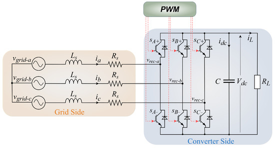
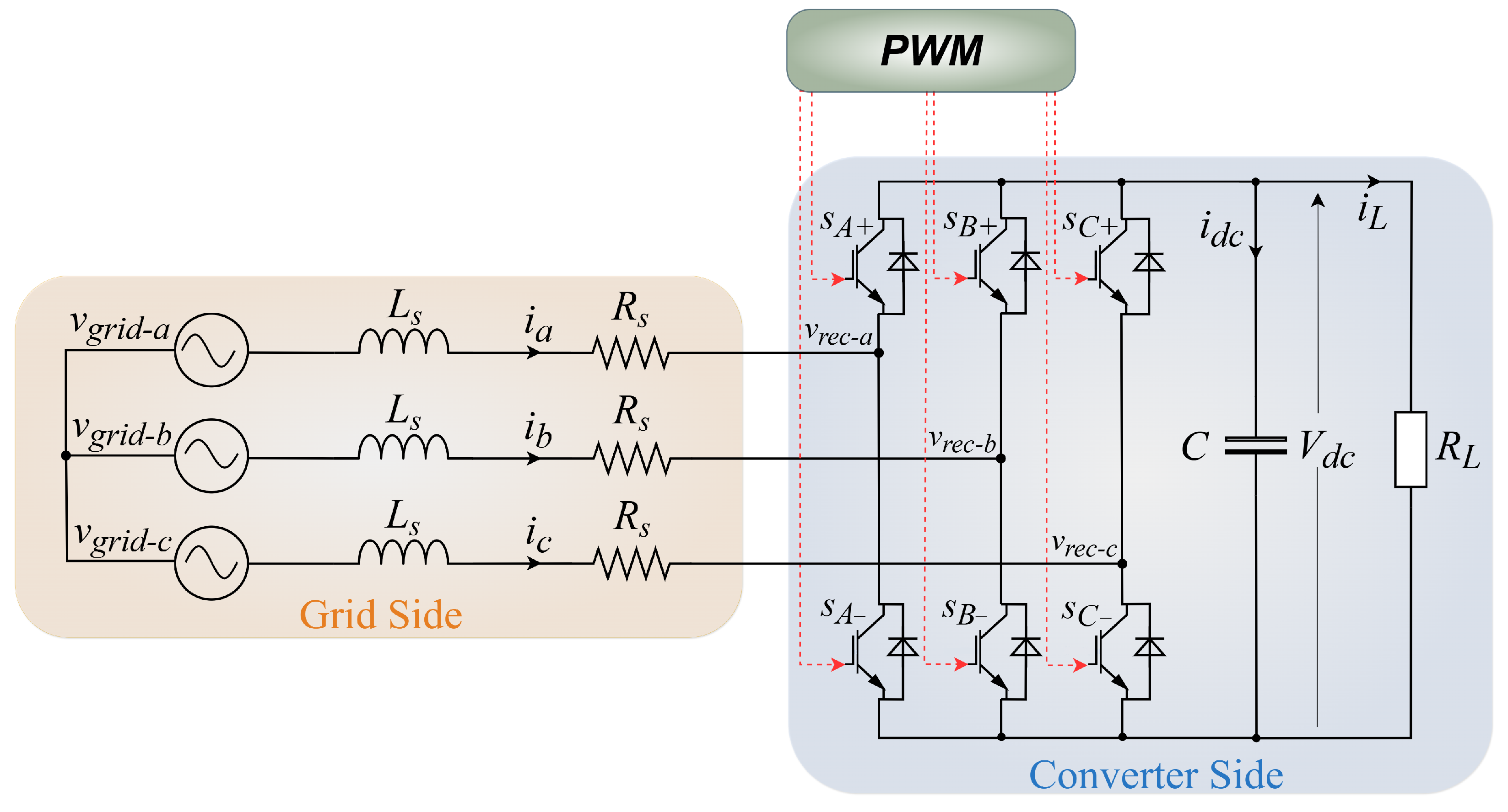
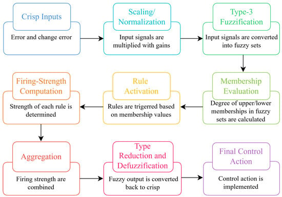
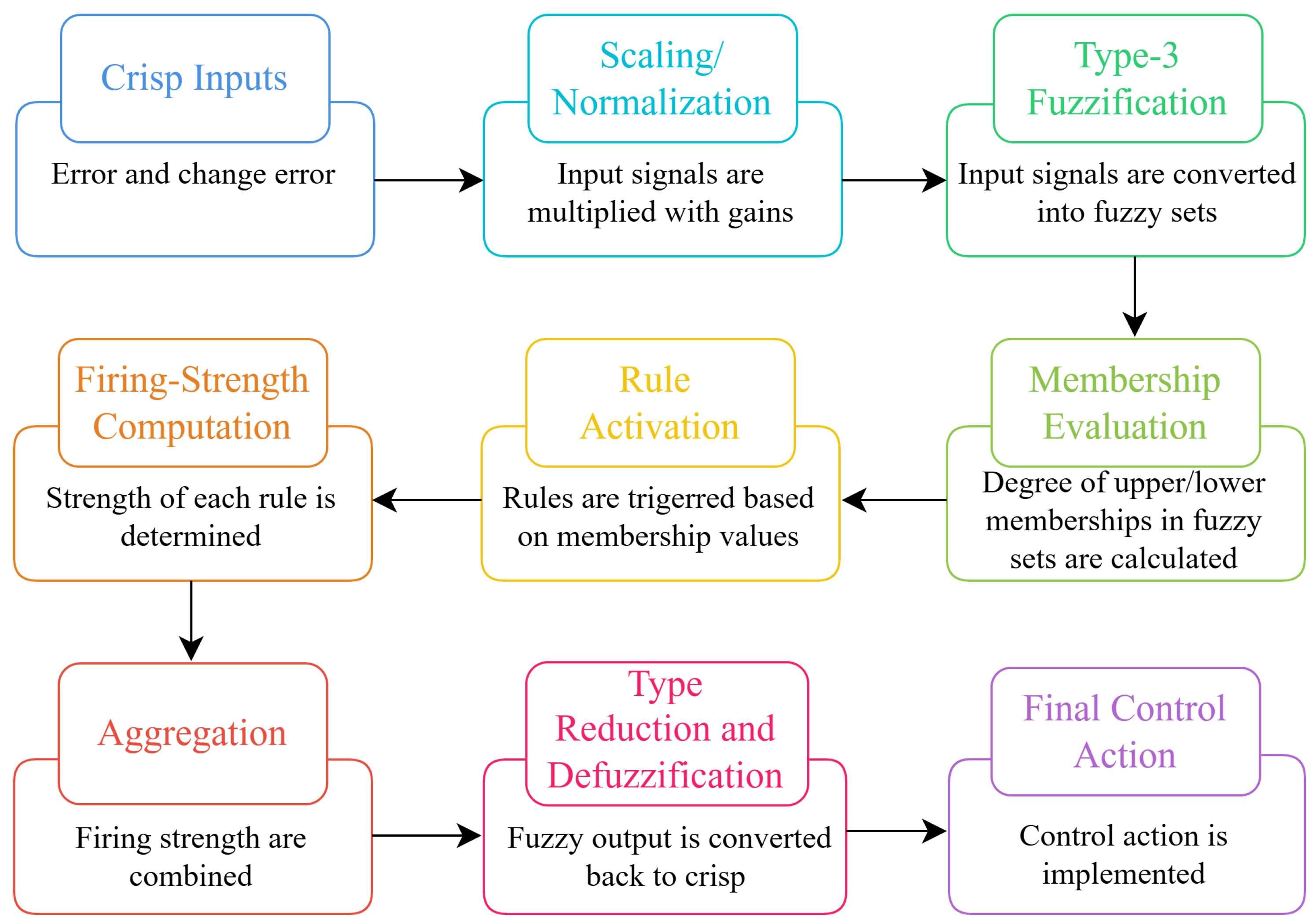
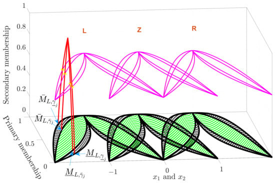
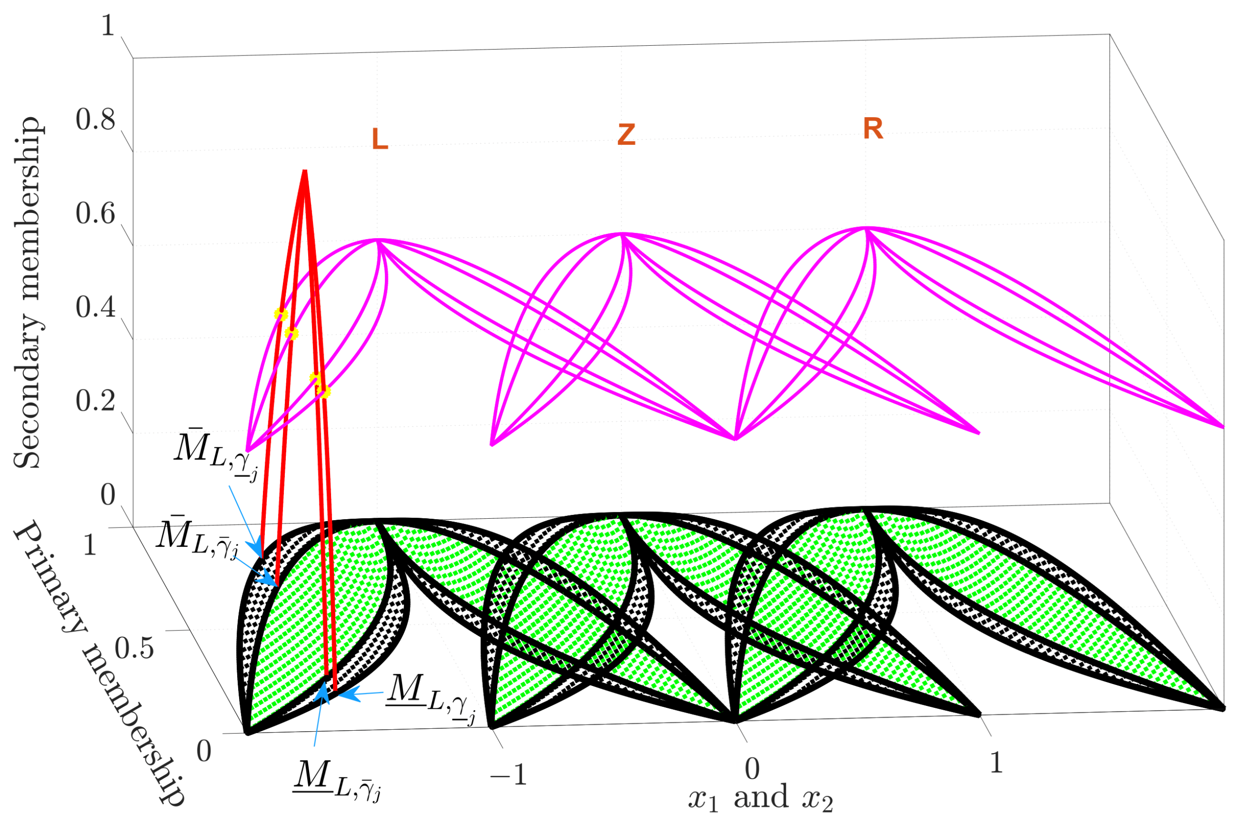
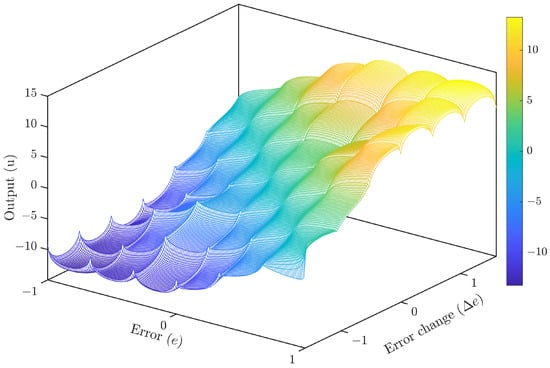
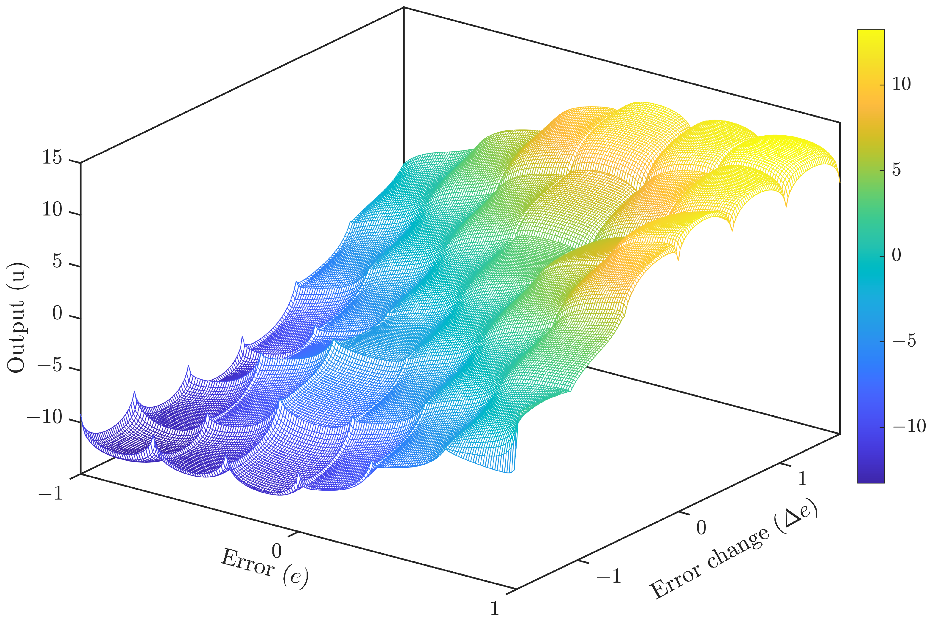
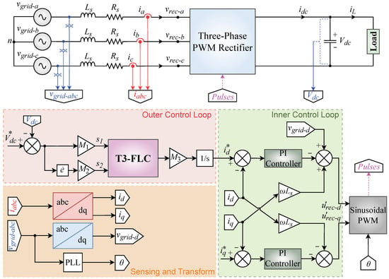
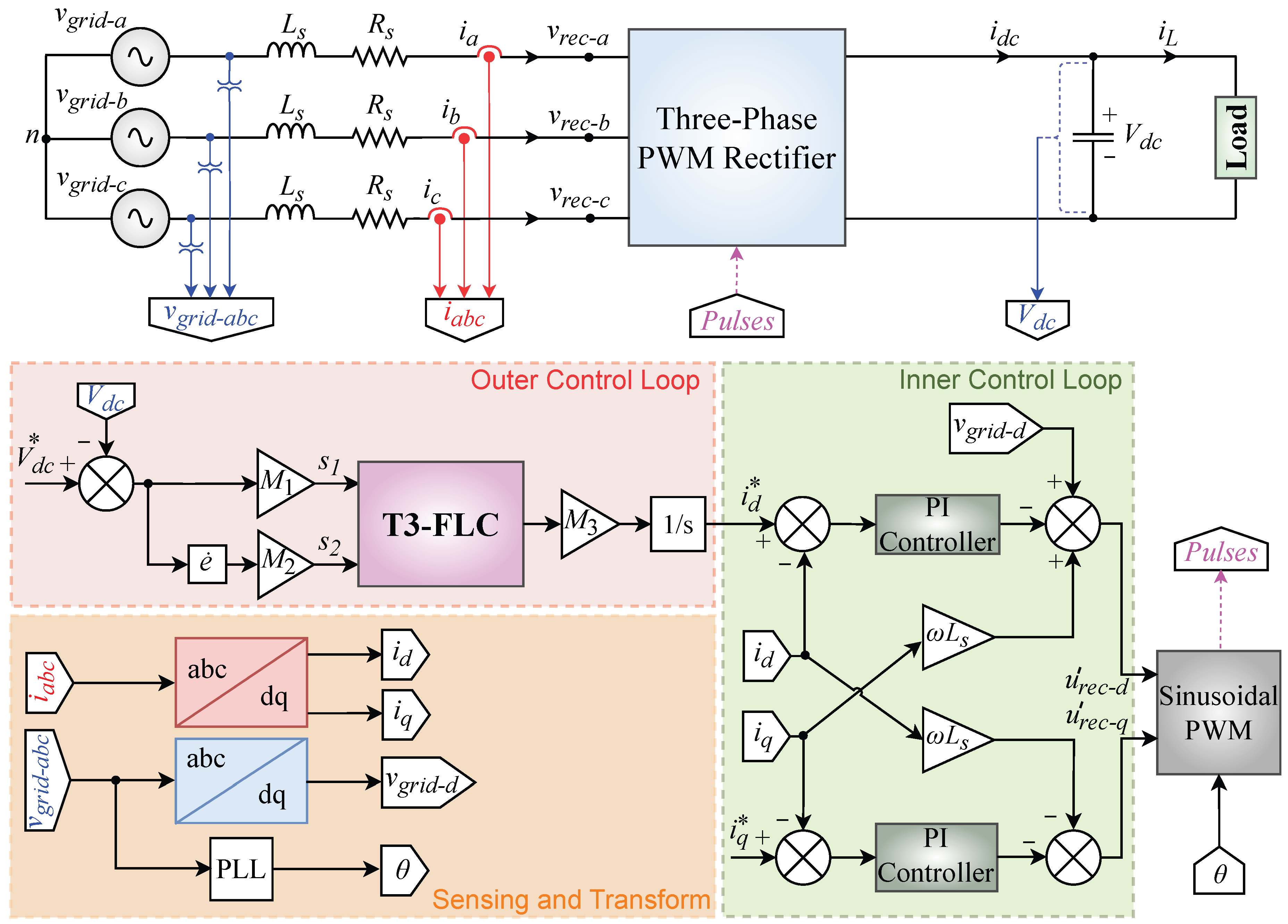
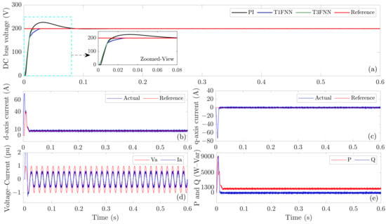
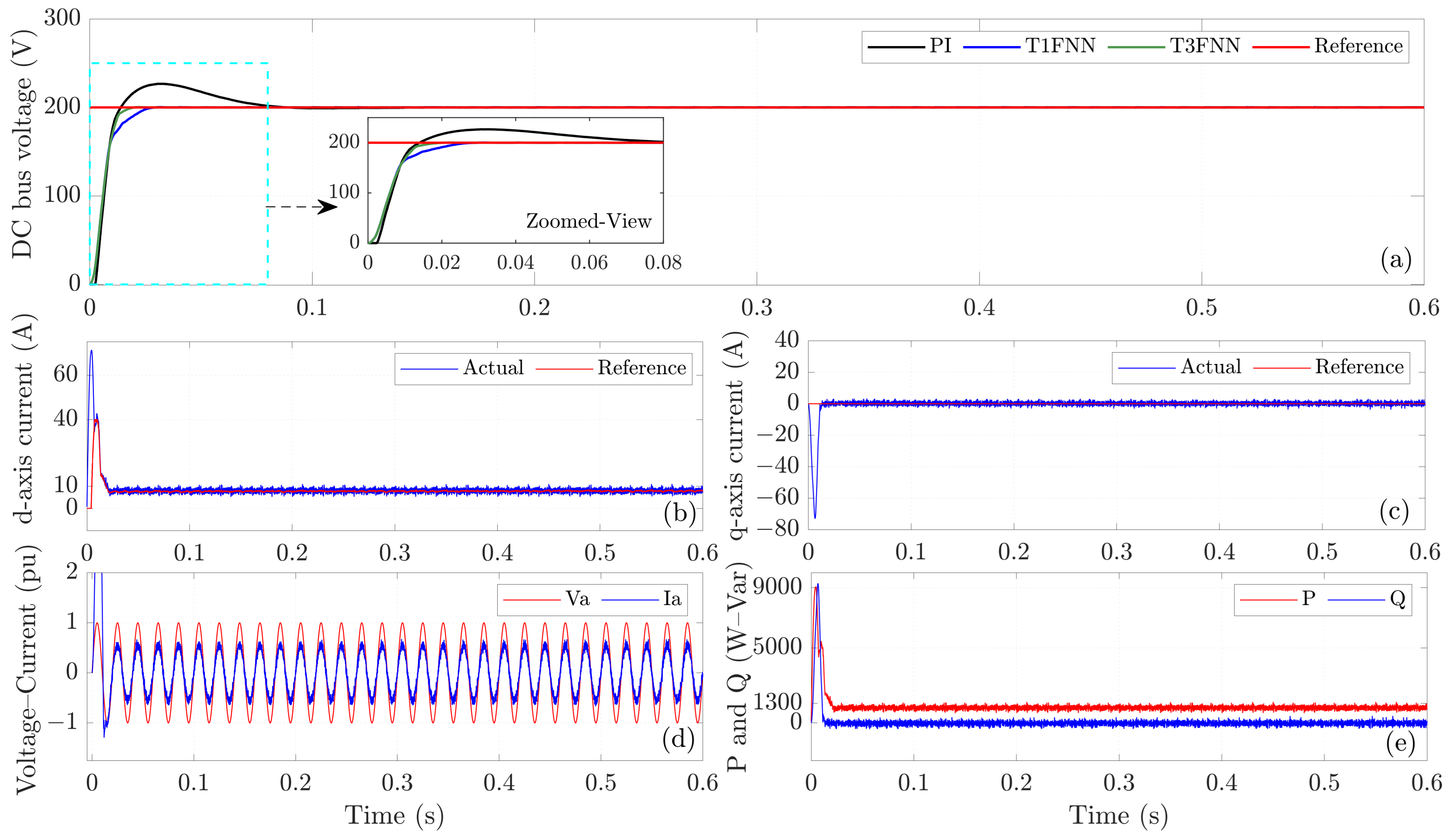
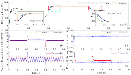
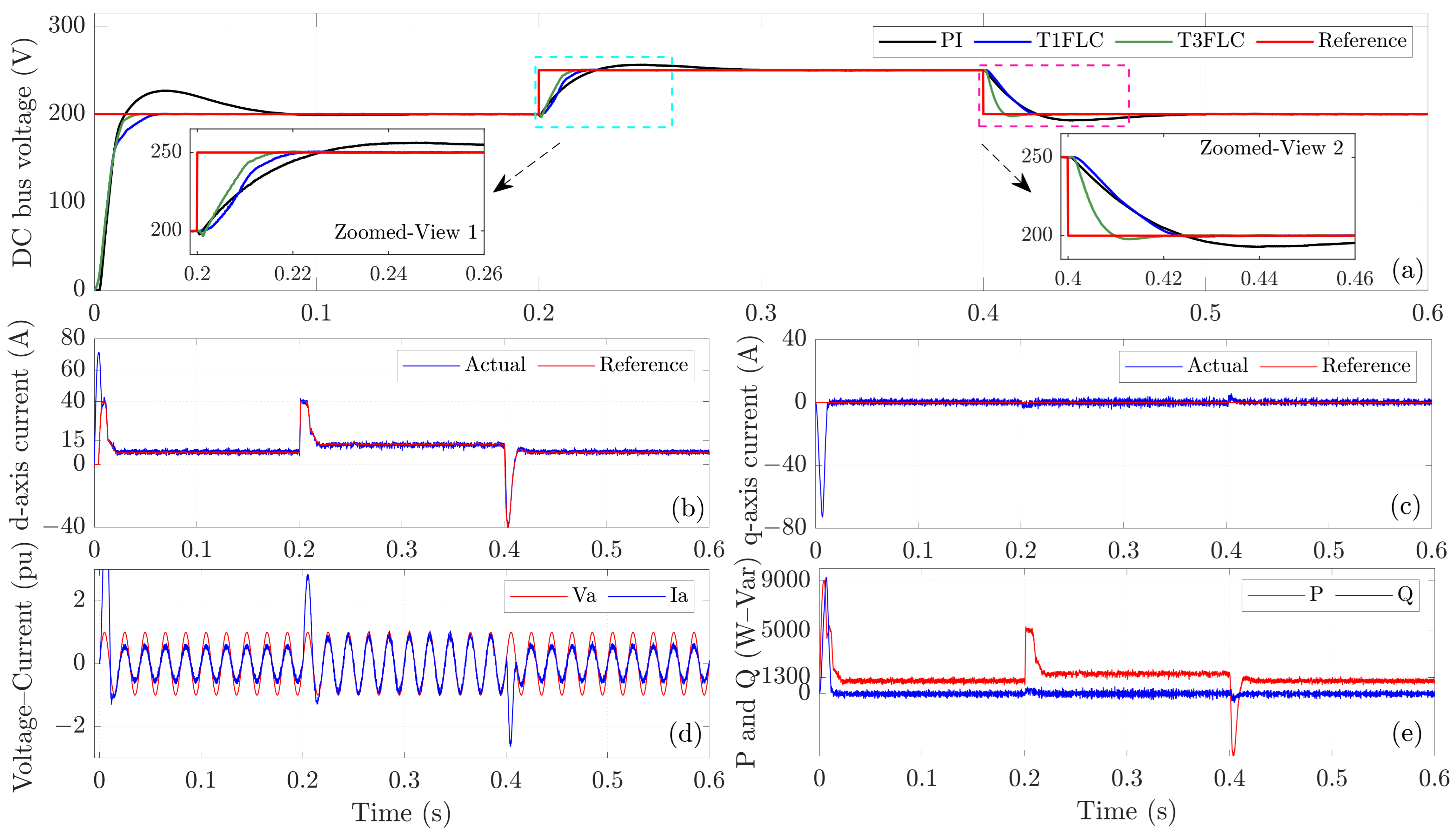
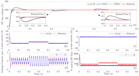
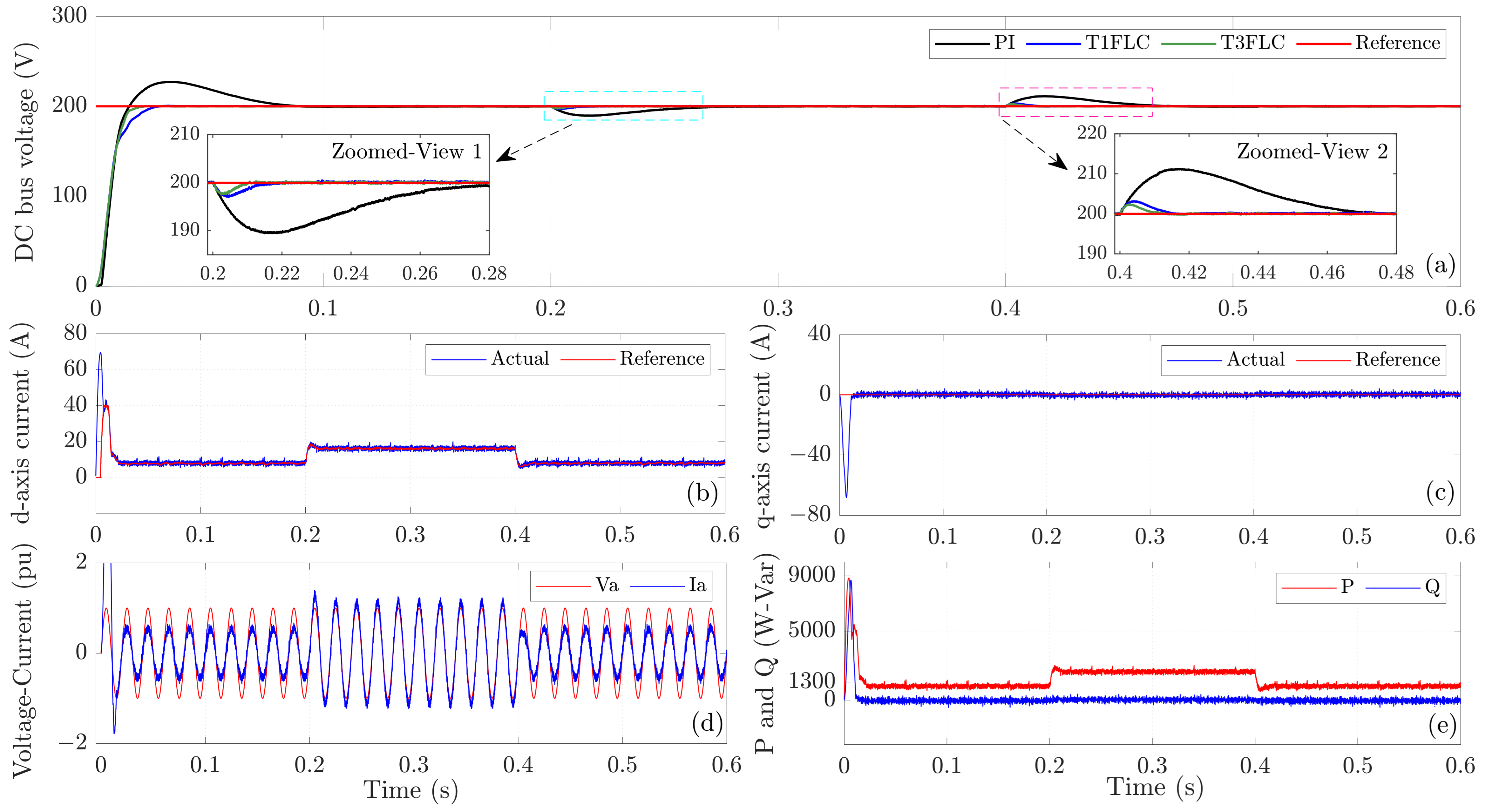
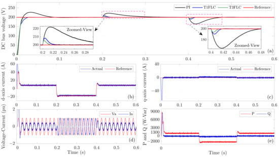
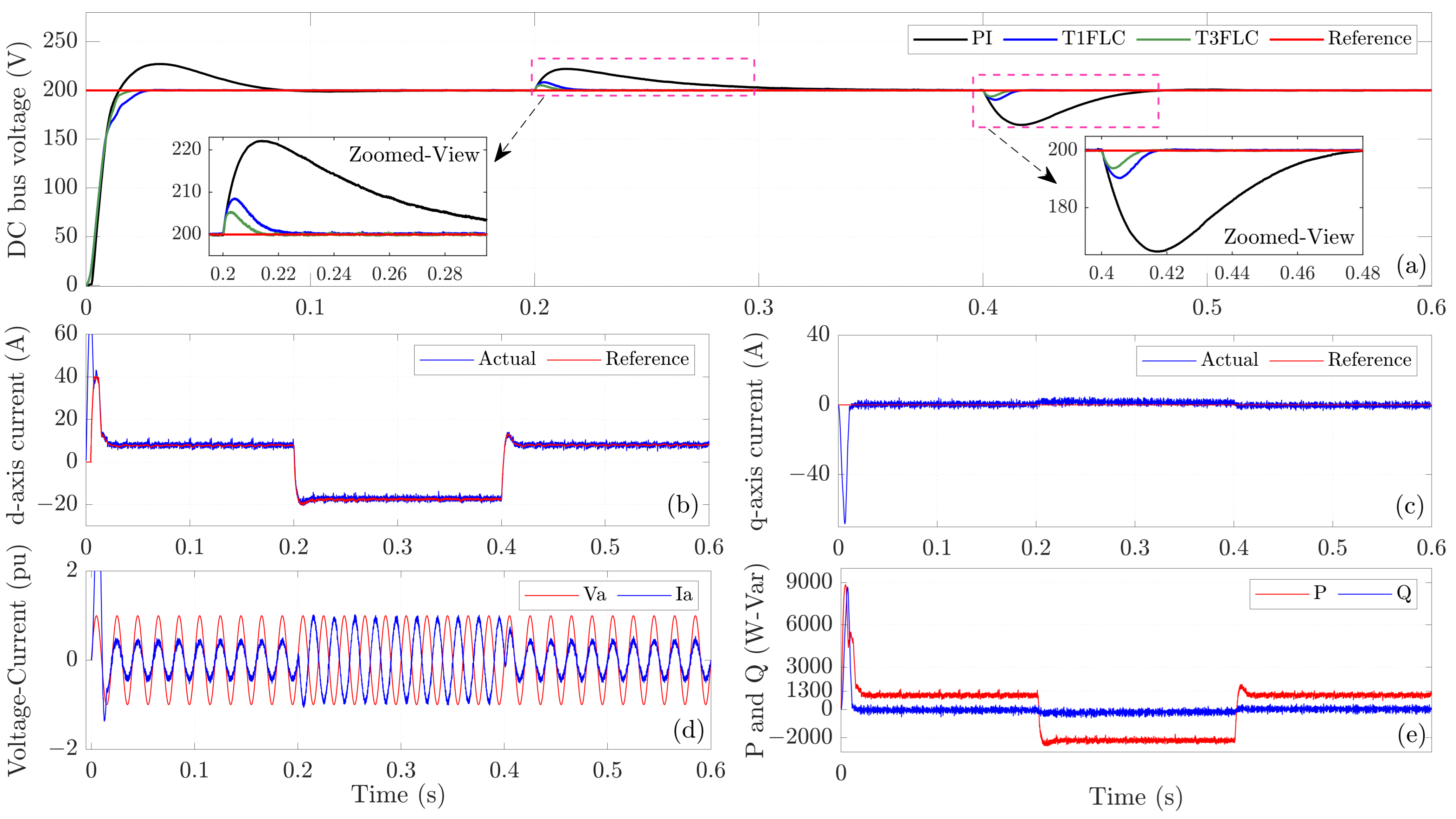
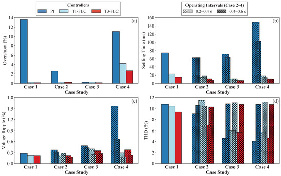
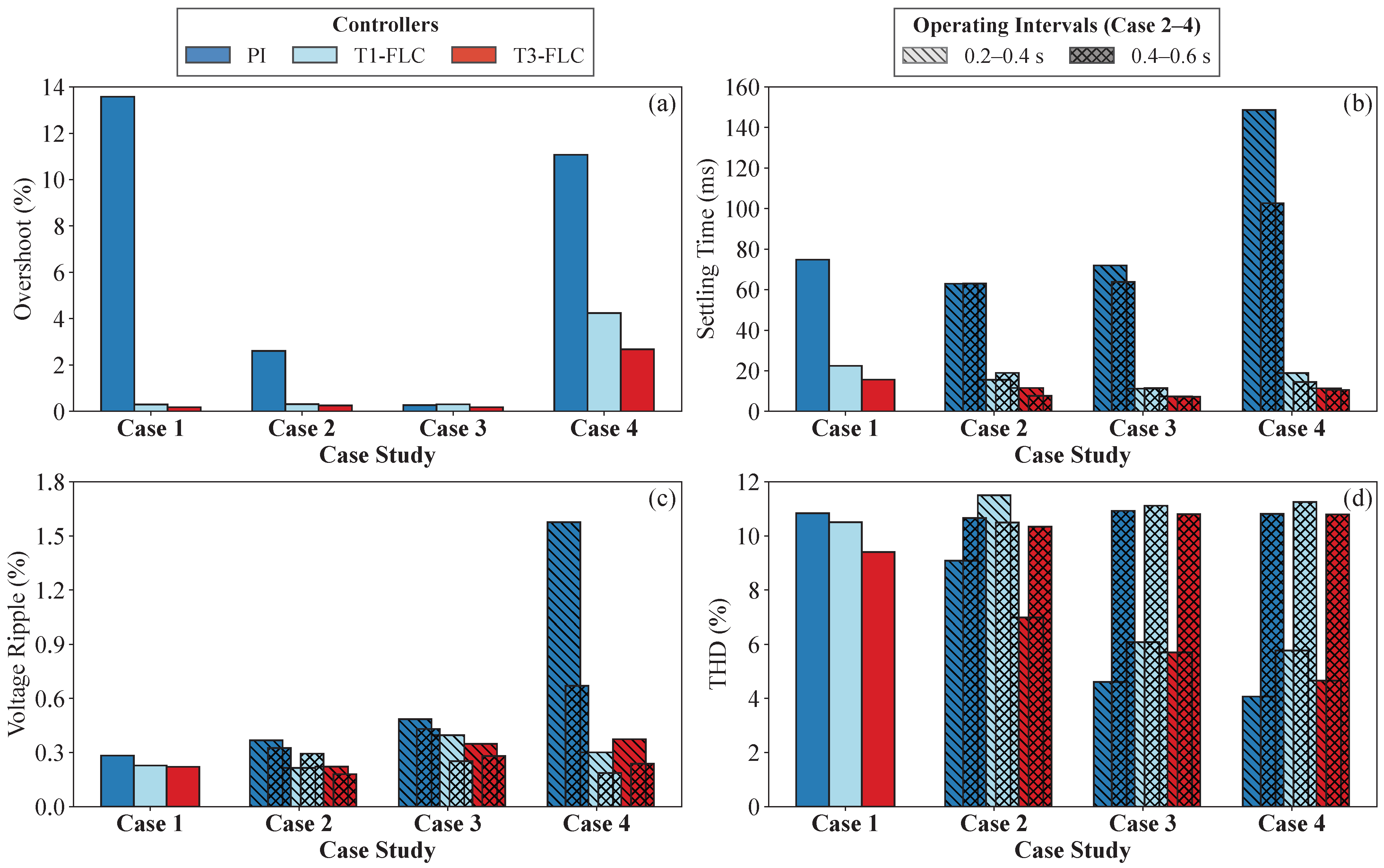
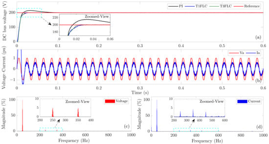
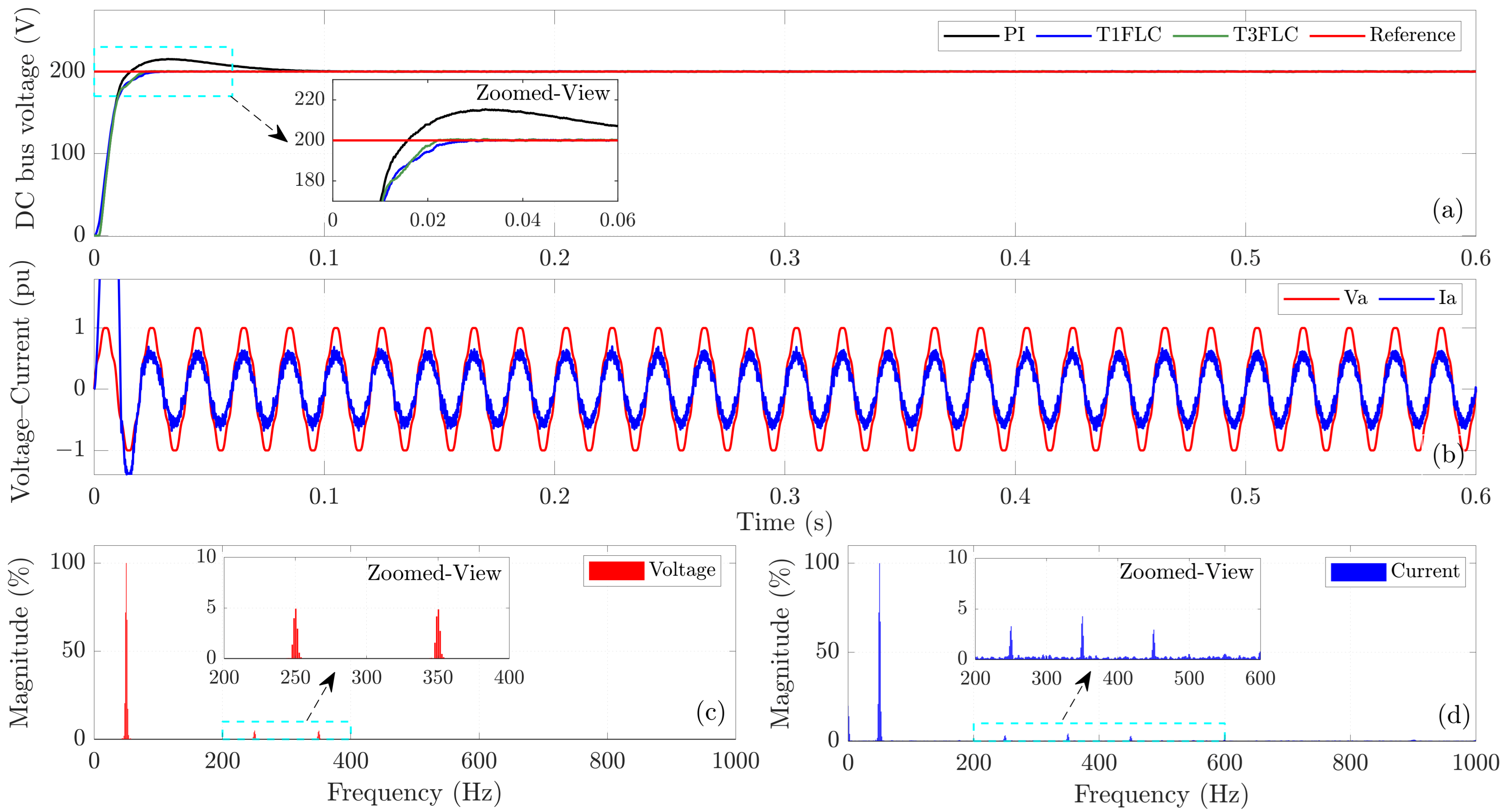
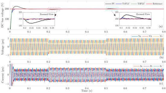
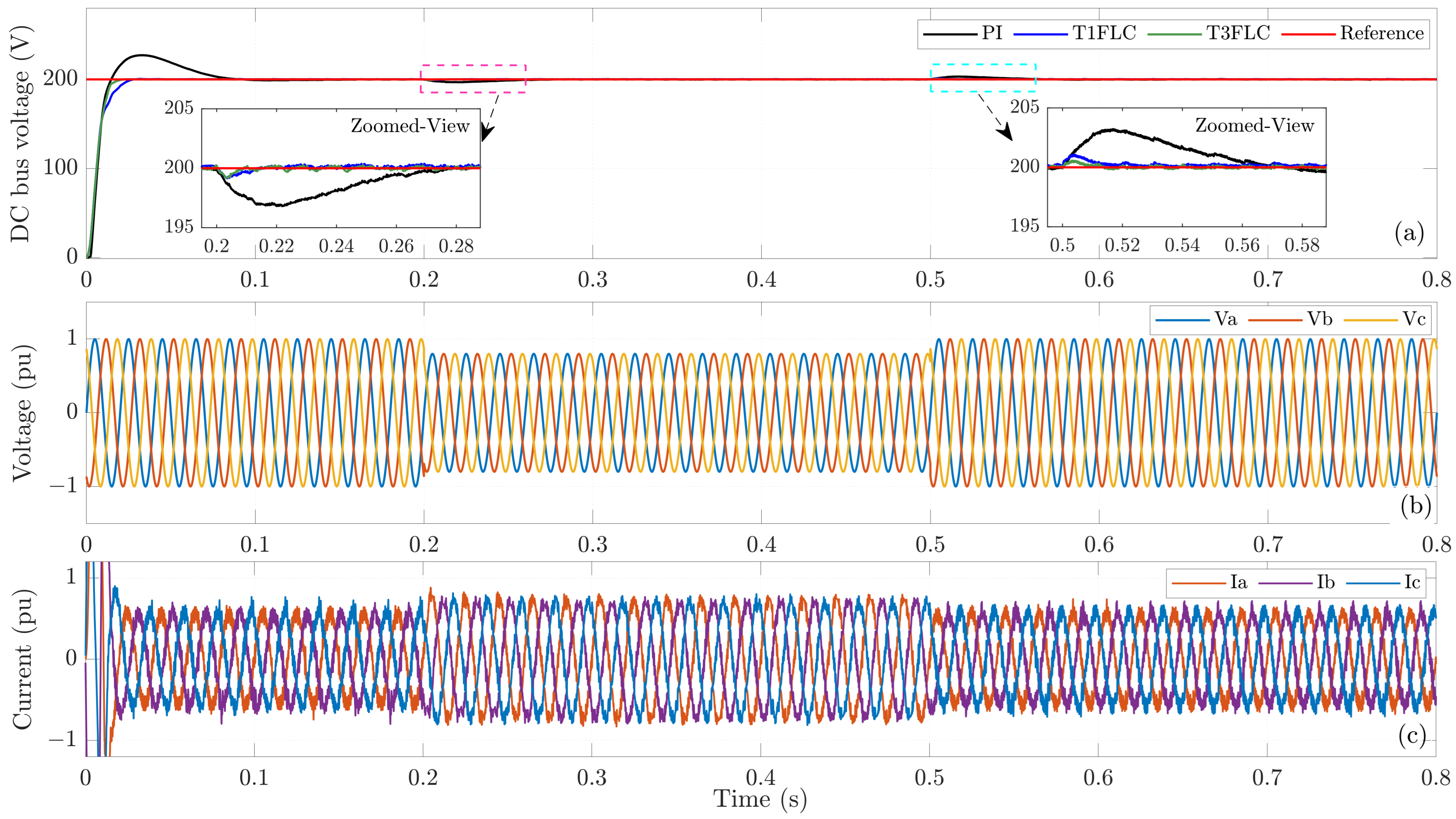
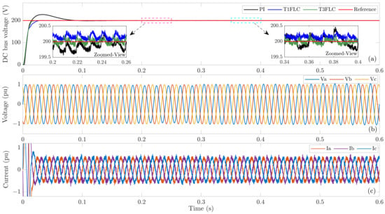
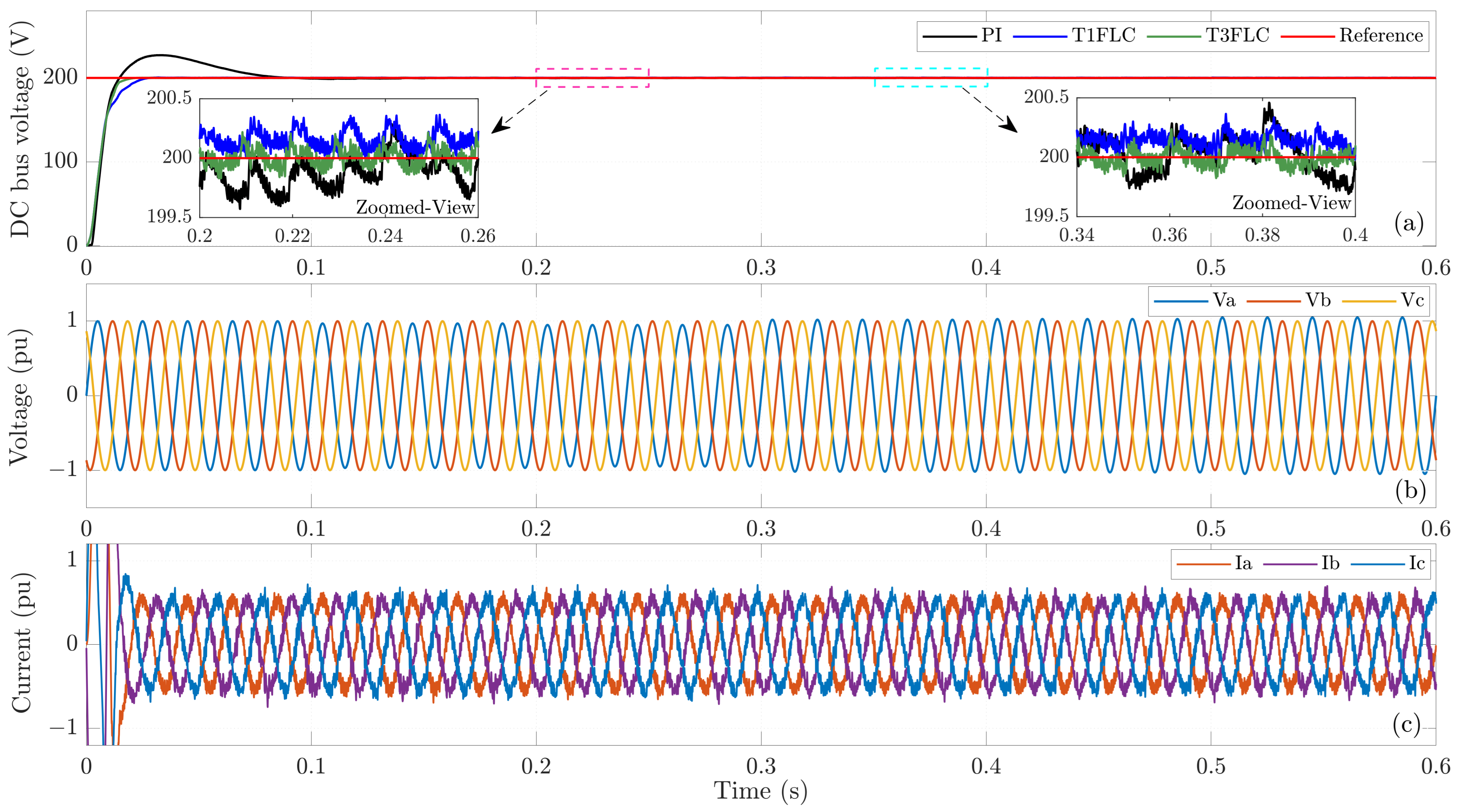

Disclaimer/Publisher’s Note: The statements, opinions and data contained in all publications are solely those of the individual author(s) and contributor(s) and not of MDPI and/or the editor(s). MDPI and/or the editor(s) disclaim responsibility for any injury to people or property resulting from any ideas, methods, instructions or products referred to in the content. |
© 2026 by the authors. Licensee MDPI, Basel, Switzerland. This article is an open access article distributed under the terms and conditions of the Creative Commons Attribution (CC BY) license.