ML-Leveraged System-Wide Fault Diagnosis Method for Wireless Power Transfer

Abstract

This paper proposes a system-wide fault diagnosis method for wireless power transfer (WPT) systems. This method enables the comprehensive fault diagnosis of key components in WPT systems by using only a single current sensor. It requires no controller upgrades, offering a cost-effective and minimally invasive solution. The fault diagnosis method is based on a support vector machine (SVM) algorithm; the Hierarchy-SVM algorithm is proposed which reduces training time to 54% and recognition time to 16.5% of those required by traditional multi-class SVM algorithms, while maintaining comparable accuracy, which was tested under the same dataset and hardware configuration. Lastly, experimental verification is conducted. The experimental results demonstrate that the proposed method achieves a more than 95% accuracy rate in identifying various faults, with an average single identification time of average 14.19 ms.

1. Introduction

As one of the promising research fields, numerous researchers and industries have recognized the great potential for the development of wireless power transfer (WPT), which has many advantages such as better flexibility, excellent shockproof performance, and strong security [1,2,3]. Typically, wireless charge will improve the flight endurance of drones and alleviate the dependence of batteries for electric vehicles (EVs) [4,5]. Despite its advantages, the widespread adoption of WPT systems is hindered by their susceptibility to various faults, such as coil misalignment, component degradation, and environmental interference [6,7].

To enhance the safety and performance of a WPT system, maintenance depends on applying the fault diagnosis algorithm. Many studies focus on faults caused by the intrusion of external objects or coil misalignment [8,9,10,11]. In [8], dual-purpose nonoverlapping coil sets for both metal object detection (MOD) on a power supply coil and the detection of position (DoP) of WPT system for EVs were proposed. To eliminate all blind zones, a simple and cost-effective symmetric sensing coil set to be used for MOD in a stationary wireless electric vehicle charger was proposed by [9]. Reference [10] proposed an accurate foreign object detection method based on the electromagnetic model of the WPT system, which demonstrates robustness against receiver coil misalignment and varying power levels, thereby supporting low-power detection before system activation. The above research only focuses on faults caused by external factors in WPT systems, but faults triggered by internal devices are relatively important. There are two main approaches to addressing internal device faults. One of them is adding additional components of the WPT system to endow it with fault-tolerant operation capability [12,13,14]. To achieve both short- and open-circuit protection, ref. [12] introduced a dual-coupled inductor–capacitor–capacitor and series (LCC-S) compensated WPT system by incorporating an additional compensation coil. In [13], a fault detection strategy was proposed, where sampling resistors were added in series with each bridge arm of the full-bridge inverter to identify MOSFET short-circuit faults. Upon fault detection, the system promptly switches from full-bridge to half-bridge operation to mitigate the issue. Ref. [14] enhanced system reliability through a multi-transmitter and multi-receiver WPT architecture, which improves fault tolerance under conditions such as single-transmitter or single-receiver open-circuit failures. Although the fault-tolerant approach can maintain the operation of the system in case of faults, it is essentially a contingency strategy aimed at mitigating rather than fundamentally solving system faults. The other approach to solving internal device faults is to locate the faulty device [15,16,17,18,19]. In [15], a rectifier protection method was proposed for series–series (SS)-compensated inductive power transfer (IPT) systems, utilizing the DC bias of fault eigenvalues to safeguard devices during rectifier open-circuit faults. To address the open-circuit fault diagnosis in inverters of WPT system, ref. [16] introduced a rough-set-theory-based (RST-based) method to diagnose and locate the open-circuit faults for the initial attempts. Additionally, extensive research has been conducted on inverter open-circuit fault diagnosis [17,18], offering valuable insights for fault diagnosis in WPT systems. In [19], a system fault state table was established to identify the soft fault of resonant capacitors. All the aforementioned studies to solve internal device faults primarily focus on addressing the individual components of the WPT system that may potentially experience failures during runtime. Consequently, establishing a comprehensive system maintenance framework through these methods is challenging because of the overly complex structure and excessive algorithmic complexity. Ref. [20] proposed a multi-type fault diagnosis method. However, the method was only verified in simulation and requires the values of all voltage and current data of the primary side and the secondary side.

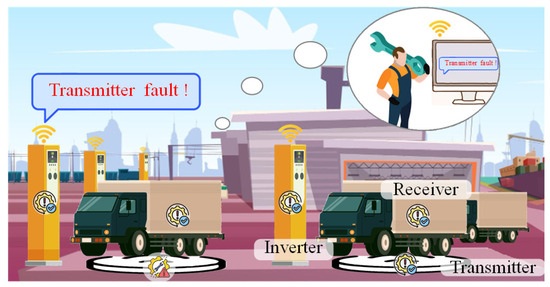
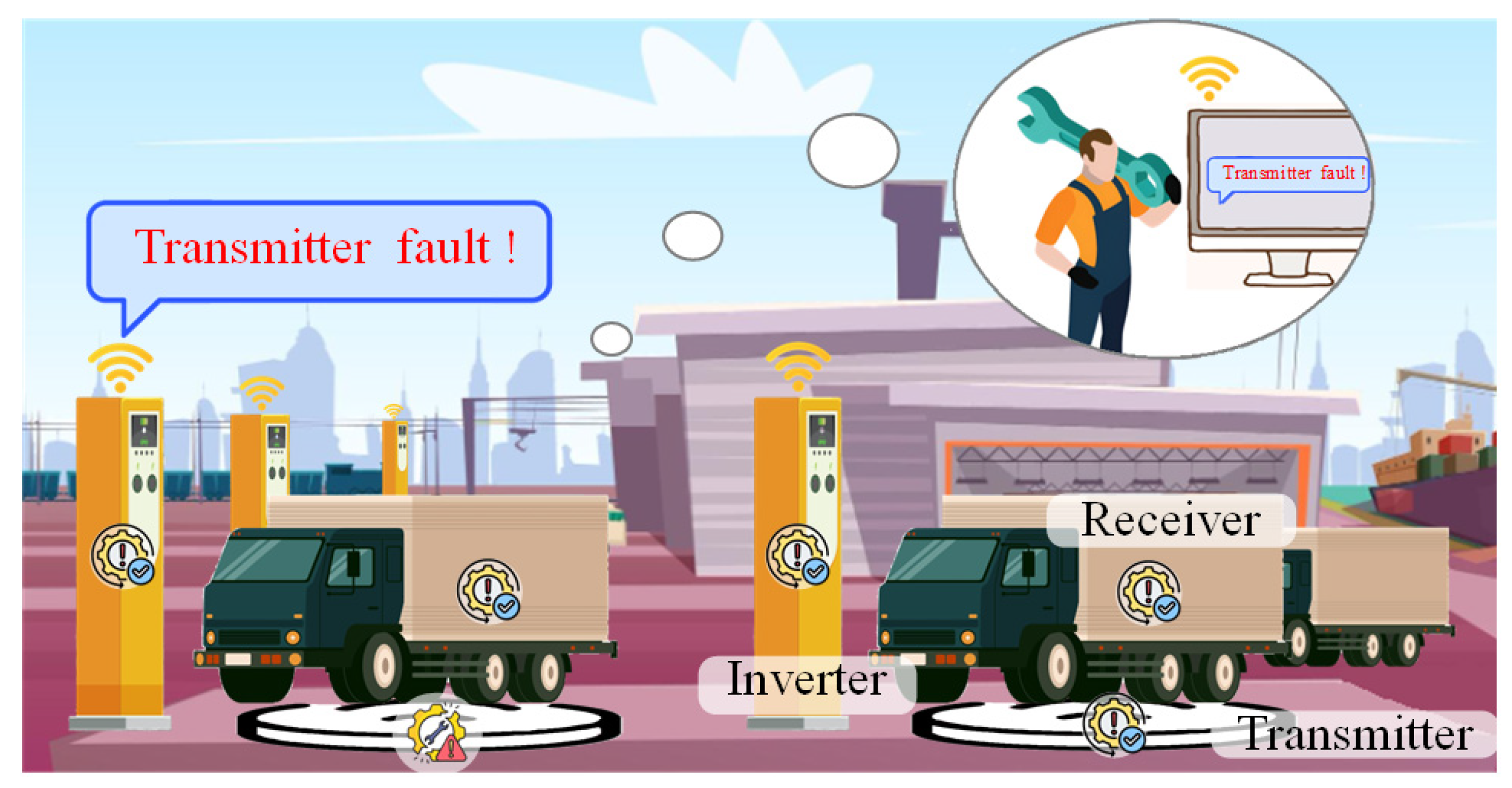
Therefore, it is necessary to develop a fault diagnosis method for internal components in WPT systems that offers a simple structure, easy implementation and the capability to diagnose multiple fault types. Accordingly, this paper proposes a primary side detection scheme for the fault diagnosis of WPT systems, aiming to establish a comprehensive system maintenance framework. Table 1 presents the comparison of fault diagnosis methods for WPT systems in the references and in this paper. The proposed method only uses a primary-side current sensor which is a standard component in most practical WPT systems. Typically, an application scenario of the proposed method is as shown in Figure 1. A maintainer can manage multiple devices simultaneously and locate the faulty device and fault type quickly at a large, unmanned cargo port. The advanced DL techniques (e.g., wavelet packet transform combined with graph learning) that offer robustness in noisy environments [21,22]. However, such methods often incur high computational costs, making them less suitable for the low-cost DSP controllers typically used in WPT systems. Therefore, the proposed system-wide fault diagnosis scheme adopts an efficient data processing method and optimized support vector machine (SVM) algorithm (Hierarchy-SVM), which facilitates straightforward deployment. The major contributions of the paper are summarized as follows:

Table 1. The comparison of fault diagnosis methods for WPT system in reference and in this paper.

Reference	Types of Diagnosable Devices in WPT System					Adding Additional Devices
	Inverter	Rectifier	Filter Capacitor	Resonant Devices	Distance
[8]	✕	✕	✕	✕	✓	Yes
[13]	✓	✕	✕	✕	✕	Yes
[15]	✕	✓	✕	✕	✕	Yes
[19]	✕	✕	✓	✕	✕	Yes
This paper	✓	✓	✓	✓	✓	No

Figure 1. Application scenario of the proposed method.

(1)

System-wide Fault Diagnosis Capability: The proposed method provides a comprehensive diagnosis of all critical components within the system such as inverter and rectifier.

(2)

Low Computational Footprint: The Hierarchy-SVM exhibits computationally efficient performance on conventional processing units like DSPs.

(3)

Communication-free Architecture: The system achieves full functionality through a primary-side current sensor alone.

2. Analysis

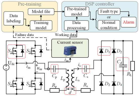
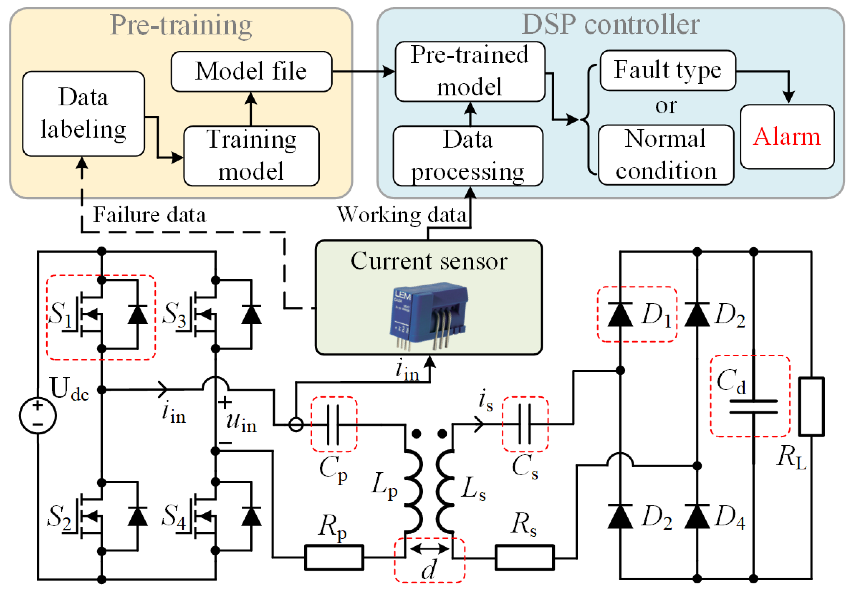
In this paper, a system-wide fault diagnosis method is proposed for WPT systems. The corresponding specific implementation and circuit model are shown in Figure 2 where L_p (L_s), R_p (R_s) and C_p (C_s) are the inductance, the equivalent resistance, and the compensation capacitance of the primary side (secondary side), respectively. Additionally, U_dc is the voltage of the dc power supply and S₁−S₄ are the switching devices of a full-bridge inverter. u_in is the input voltage and i_in is the input current. i_s is the secondary current. D₁−D₄ are the diodes of the rectifier and C_d is the filter capacitor. d is the distance between the transmitter (TX) and receiver (RX). R_L is the resistance of the load. The system applies S–S resonant network [23]. In normal conditions, the network satisfies.

$$\left\{\begin{array}{c}1/2j\pi f{C}_{\mathrm{p}}+j\omega L_{\mathrm{p}}=0\\ 1/2j\pi f{C}_{\mathrm{s}}+j\omega L_{\mathrm{s}}=0\end{array}\right.$$

(1)

where f is the working frequency. The equivalent load of the rectifier with R_L R_eq, primary side impedance Z_p and secondary side impedance Z_s are given as

$$\left\{\begin{array}{c}{R}_{\mathrm{eq}}=8R_{\mathrm{L}}/{\pi }^2\\ Z_{\mathrm{p}}=1/2j\pi f{C}_{\mathrm{p}}+j\omega L_{\mathrm{p}}+R_{\mathrm{p}}\\ Z_{\mathrm{s}}=1/2j\pi f{C}_{\mathrm{s}}+j\omega L_{\mathrm{s}}+R_{\mathrm{eq}}\end{array}\right.$$

(2)

Figure 2. A circuit of the WPT system and the specific implementation of the proposed system-wide fault diagnosis method.

According to Kirchhoff’s voltage law, the equation of the primary circuit can be given as

$$u_{\mathrm{in}}=i_{\mathrm{in}}(Z_{\mathrm{p}}+{\displaystyle \frac{4{\pi }^2{f}^2{M}^2}{Z_{\mathrm{s}}}})$$

(3)

where M is the mutual inductance between TX and RX, which is related to d.

The operative mode of inverter changes the u_in directly. According to (2) and (3), the value of C_p (C_s) changes the state of resonance in primary (secondary) circuits, respectively and leads to the change in i_in indirectly. The value of R_eq is influenced by the operating state of the rectifier and C_d which also changes i_in indirectly. By Faraday’s law of induction, d is a parameter that affects M which is another influencing factor of i_in. Through the above analysis, any deviation from the normal working state of the main devices can be reflected in i_in. Therefore, the proposed method adopts a current sensor to measure i_in to observe the working status of the main devices.

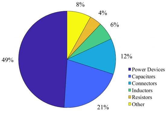
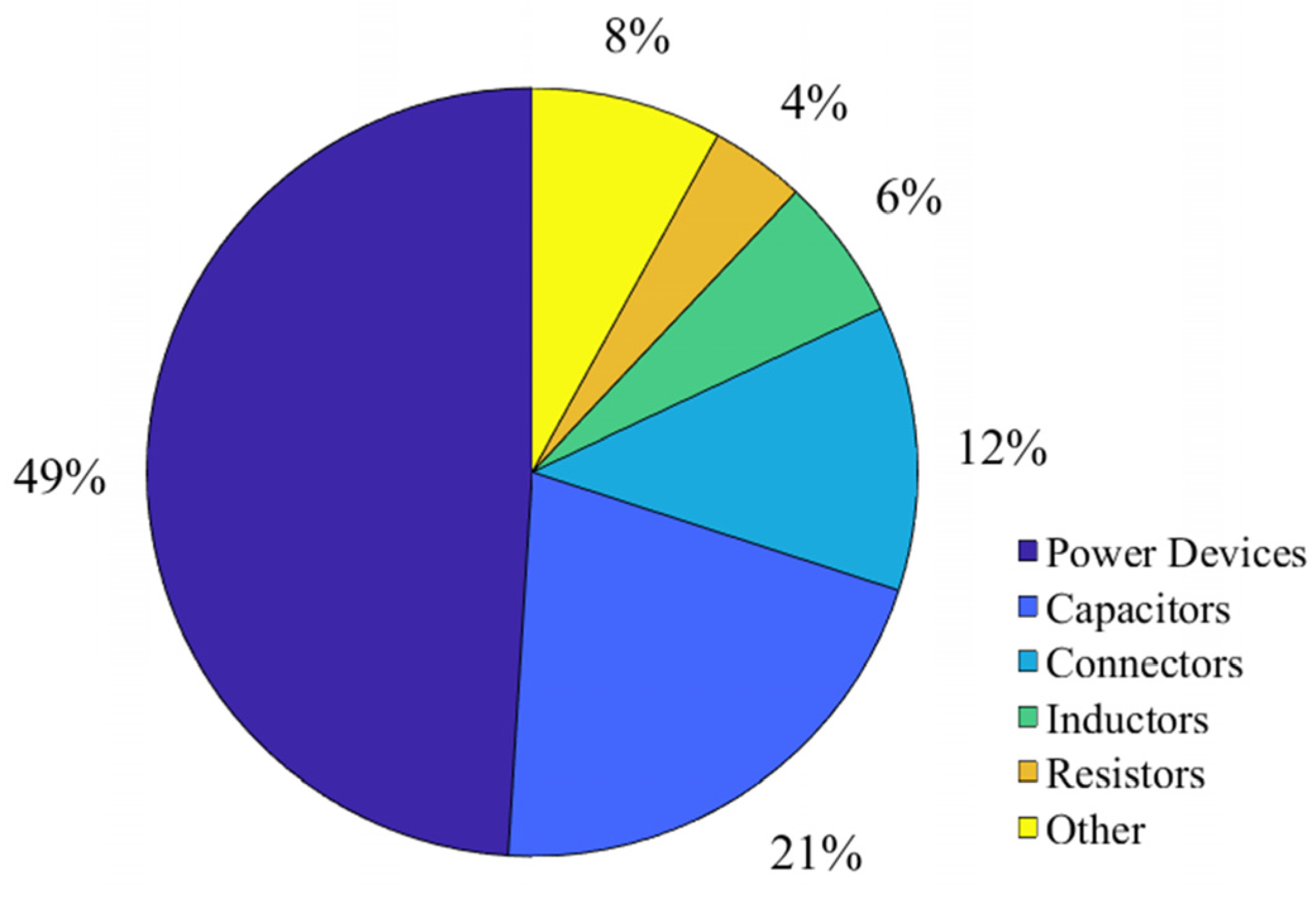
The devices of WPT systems can be divided into two categories, which are resonant devices (L_p, L_s, C_p and C_s) and power devices (S₁−S₄, D₁−D₄ and C_d). The resonant devices mainly experience parameter drift faults due to aging, and the power devices mainly experience open-circuit and short-circuit faults. Among them, the failure rate of inductors is relatively low, while the failure rates of other components can account for more than 70% [6], which is displayed in Figure 3. M is also an important parameter that affects the performance of the WPT system, so d should also be considered.

Figure 3. Failure distribution of devices in WPT systems [6].

Based on the above analysis, the proposed method identifies ten classes of fault including one of S₁−S₄ open-circuit (S_n-open), an increment of the value of C_p (C_p-inc), a decrement of the value of C_p (C_p-dec), a change in d (d-cha), an increment of the value of C_s (C_s-inc), a decrement of the value of C_s (C_s-dec), one of D₁−D₄ open-circuit (D_n-open), one of D₁−D₄ short-circuit (D_n-short), C_d open-circuit (C_d-open), and C_d short-circuit (C_d-short), which are also selected by the red dotted box in Figure 2. Set capacitance value is offset from the normal value of 220 pF and above, d value is offset from the normal value of 1 cm and above to the fault states, which have a significant impact on the WPT system when the value deviates beyond that. The specific phenomena will be demonstrated in the Section 4.

The implementation of system-wide fault diagnosis method is divided into two blocks as shown in Figure 2. Training the model beforehand can effectively improve the performance of procedure with limited computing resource of the controller. The detail about the data processing and model training will be elaborated in following parts.

3. Fault Diagnosis Method

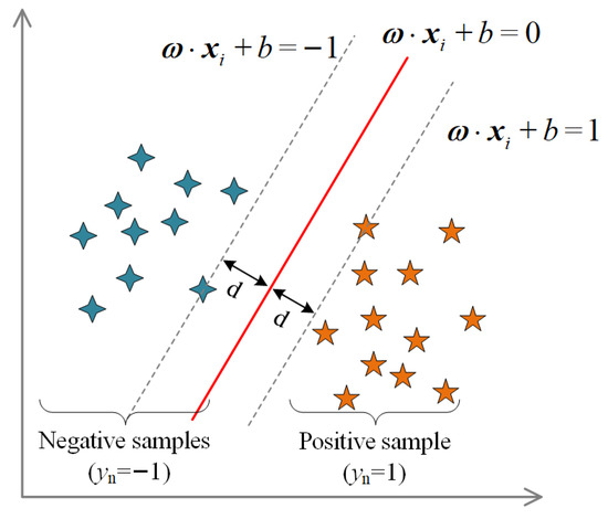
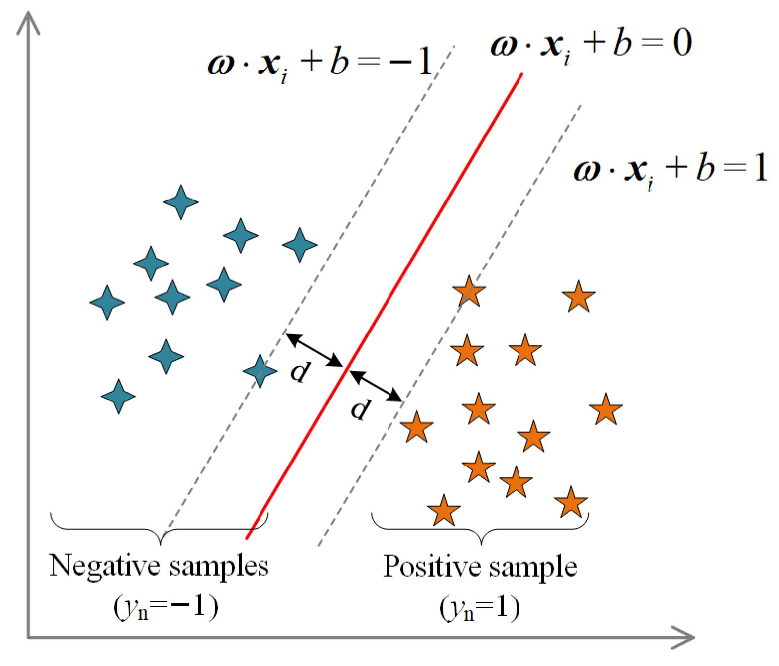
The proposed system-wide fault Diagnosis method is based on optimized multi-class SVM algorithm. Compared to models such as CNN and RNN, SVM demonstrates superior generalization capability on small-sample fault data and is less prone to overfitting. Additionally, its lower inference computational overhead aligns better with the real-time and resource constraints of embedded systems [24]. The traditional SVM algorithm was proposed to solve binary classification problems [25]. Then, multi-class classifications can be performed based on the binary classification SVM algorithm. The key idea of the SVM algorithm is to find the maximum distance between two types of samples as shown in Figure 4.

Figure 4. The structure of binary SVM model.

The training samples can be given as

$$\left\{\left({\mathit{x}}_1,y_1\right),\left({\mathit{x}}_2,y_2\right),\dots ,\left({\mathit{x}}_i,y_i\right)\right\}$$

(4)

where x_i is the feature vector in the high-dimensional space and y_i = {−1, 1} (i = 1, 2, …, n) represents the positive sample or the negative sample. Decision equation (the red line in Figure 4) can be given as

$$\mathsf{\omega }\cdot {\mathit{x}}_i+b=0$$

(5)

where ω is the weight vector, and b is the linear intercept. All the training samples should satisfy

$$\left\{\begin{array}{ll}\mathsf{\omega }\cdot {\mathit{x}}_i+b\ge 1\hfill & \forall y_i=1\hfill \\ \mathsf{\omega }\cdot {\mathit{x}}_i+b\le -1\hfill & \forall y_i=-1\hfill \end{array}\right.$$

(6)

which is the constraint. The problem of SVM optimization solution is to find the maximum margin δ between two types of samples. The δ can be calculated as

$$\delta =1/‖\mathsf{\omega }‖$$

(7)

Then, the optimization problem can be transformed as

$$\begin{array}{ll}{\min }_{\mathsf{\omega },b}\hfill & {\displaystyle \frac{1}{2}}\Vert \mathsf{\omega }{\Vert }^2\hfill \\ s.t. \hfill & y_i({\mathsf{\omega }}^T{\mathbf{x}}_i+b)\ge 1,\hspace{1em}i=1,2,\dots ,n\hfill \end{array}$$

(8)

By introducing the Lagrange function, the constrained optimization problem is transformed into an unconstrained optimization problem and solved through the Karush–Kuhn–Tucker (KKT). The optimization problem can be transformed as

$$\begin{array}{ll}{\min }_{\alpha }\hfill & {\displaystyle \sum _{i=1}^n{\alpha }_i}-{\displaystyle \frac{1}{2}}{\displaystyle \sum _{i,j=1}^n{\alpha }_i}{\alpha }_j{y}_i{y}_j{x}_i^T{x}_j\hfill \\ s.t. \hfill & {\alpha }_i>0,\hspace{1em}i=1,2,\dots ,n\hfill \\ & {\displaystyle \sum _{i=1}^n{\alpha }_i}{y}_i=0\hfill \end{array}$$

(9)

where α_i is the Lagrangian multiplier. If the training samples are linearly separable like the samples of Figure 4, the final hyperplane equation can be given as

$$f(\mathit{x})={\displaystyle \sum _{i=1}^n{\alpha }_i}{y}_i{\mathit{x}}_i^T\mathit{x}+b$$

(10)

However, due to the complex electromagnetic relationship, the data in this paper are linearly inseparable. Therefore, for linear inseparability, a nonlinear mapping can be used to map the data to the feature space and use a linear learner in the feature space. The classification function is transformed as follows:

$$f(\mathit{x})={\displaystyle \sum _{i=1}^n{\alpha }_i}{y}_{i}K({\mathit{x}}_i,\mathit{x})+b$$

(11)

where K(x_i, x) is the kernel function. The optimization problem also needs to be updated as

$$\begin{array}{ll}{\min }_{\alpha }\hfill & {\displaystyle \sum _{i=1}^n{\alpha }_i}-{\displaystyle \frac{1}{2}}{\displaystyle \sum _{i,j=1}^n{\alpha }_i}{\alpha }_j{y}_i{y}_{j}K({\mathit{x}}_i,{\mathit{x}}_j)\hfill \\ s.t.\hfill & {\alpha }_i>0,\hspace{1em}i=1,2,\dots ,n\hfill \\ & {\displaystyle \sum _{i=1}^n{\alpha }_i}{y}_i=0\hfill \end{array}$$

(12)

In SVM, the choice of kernel function significantly affects classification performance. Commonly used kernel functions include the linear kernel, polynomial kernel, radial basis function (RBF) kernel, and sigmoid kernel. In this study, the RBF kernel is adopted. The RBF kernel is particularly advantageous due to its ability to handle nonlinearly separable data and its localized response characteristics, making it highly effective in capturing complex data distributions with fewer hyperparameters. The RBF is defined by

$$K({\mathit{x}}_i,{\mathit{x}}_j)=\exp \left\{-{\displaystyle \frac{\Vert {\mathit{x}}_i-{\mathit{x}}_j{\Vert }^2}{{\sigma }^2}}\right\}$$

(13)

where σ is the width of RBF kernel. The method proposed in this paper is also based on the traditional SVM algorithm. The hyperparameters for the RBF kernel SVM, specifically the penalty parameter C and kernel coefficient γ, were tuned using Grid Search with 5-fold cross-validation. The search space was defined as C ∈ [10⁻², 10³] and γ ∈ [10⁻⁴, 10²]. The optimal parameters yielding the highest validation accuracy were selected for each binary classifier in the hierarchy. It is optimized through the method to be mentioned below.

3.1. Data Processing and Collection Method

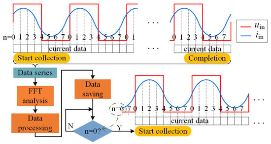
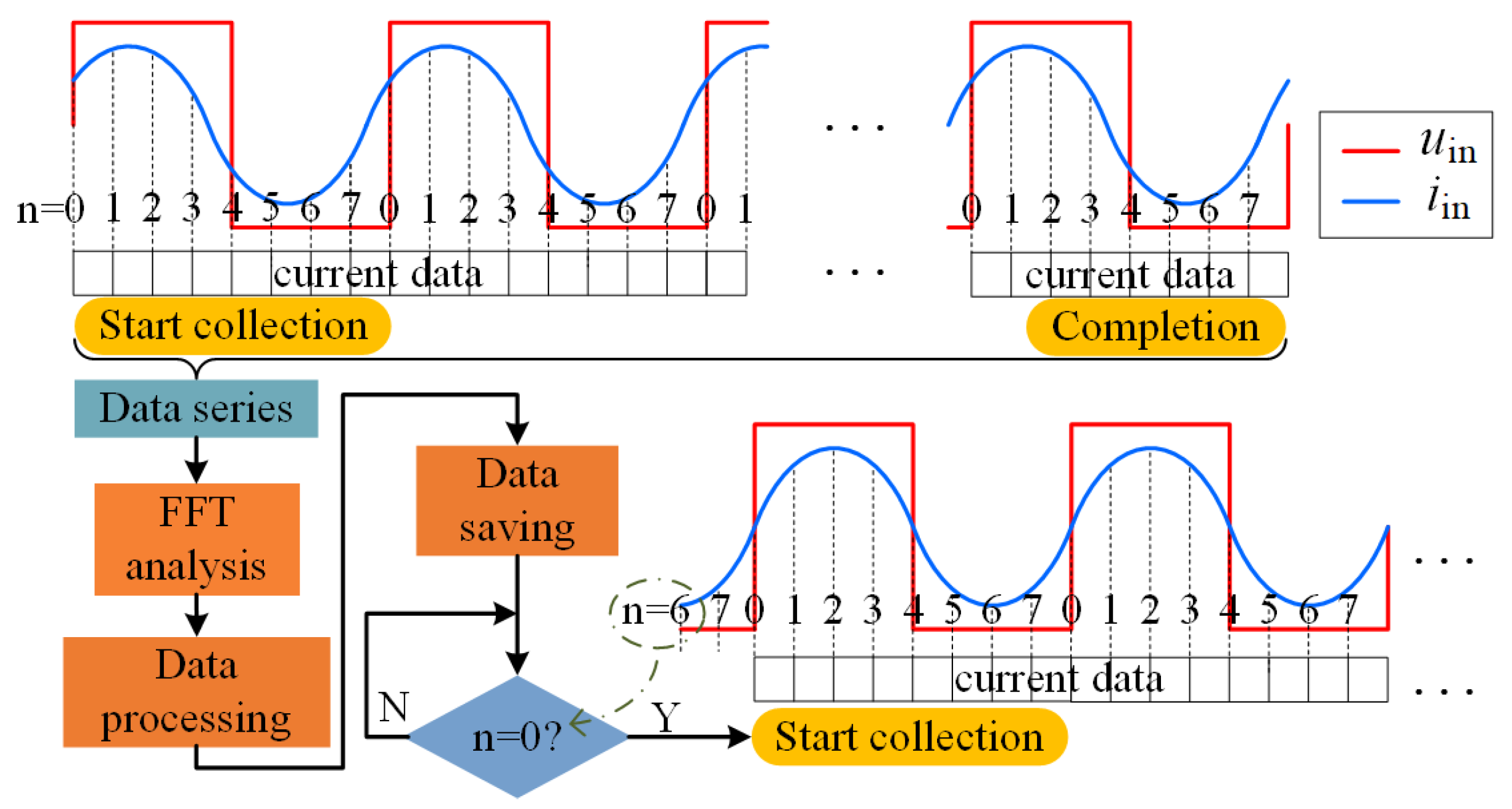
As the whole system only has one current sensor, it is necessary to design an artful data processing method to obtain more information with limited data to improve recognition accuracy. Usually, the value of U_dc is set previously. Then, the ideal waveform of u_in is gained on the premise of the known switching point of S₁−S₄ without any voltage sensor. One other thing to note is that the timeline of the collected data series of i_in needs to be aligned with that of the simulated waveform of u_in to obtain the accurate phase information of u_in and i_in. The specific method to achieve that is shown in Figure 5. The zero point of loop counter n is aligned with the rising edge of u_in to ensure the first data of the current data series is collected in time. After FFT analysis, the phase difference α_d between the fundamental component of u_in and the fundamental component of i_in can be given as

$${\alpha }_d={\alpha }_u-{\alpha }_i+{\alpha }_e$$

(14)

where α_u is the phase of the fundamental component of u_in calculated previously, α_i is the phase of the fundamental component of i_in, and α_e is the phase delay caused by collection. After data processing, the feature vector x can be given as

$$\mathit{x}=({\mathrm{I}}_{in},{\alpha }_d)$$

(15)

where I_in is the amplitude of the fundamental current wave of i_in. The feature vector x defined in (15) has a dimension of two, consisting of the fundamental current amplitude and the phase difference. These features are extracted via FFT analysis from a data window (100 kHz operating frequency, 800 kHz sampling frequency, 50 data points per FFT window). The SVM classifier processes each extracted feature vector independently as a single diagnosis instance. The system performs periodic diagnoses where each cycle yields one 2-dimensional input vector for classification. This approach ensures computational efficiency suitable for real-time embedded implementation.

Figure 5. Flow diagram of data collection and process.

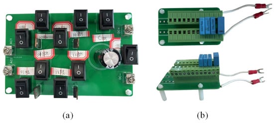
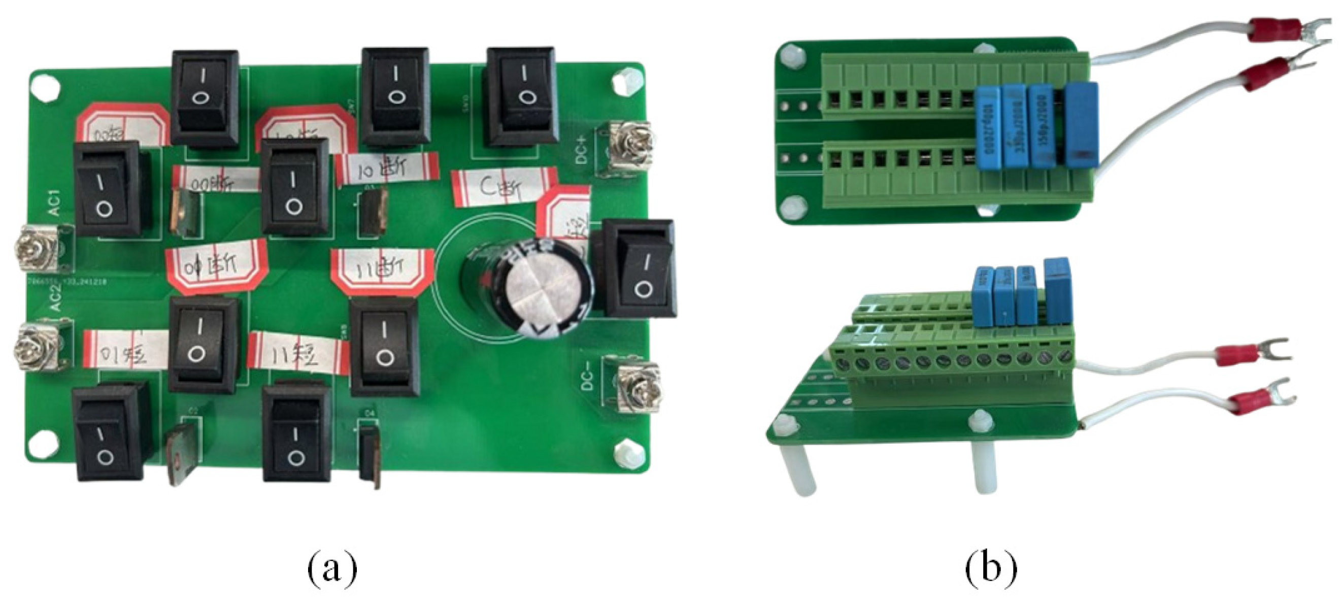
All the fault data is collected from the experimental prototype. The DSP controller collects the fault data, processes it and uploads it to the computer to build a fault data set. S_n-open data is collected by setting the level of PWM signal to low. The open-circuit and short-circuit faults of D₁−D₄ and C_d are simulated by controlling the switching states of switches on a specially designed rectifier PCB as shown in Figure 6a. The values of C_p and C_s are tunable by adding or subtracting capacitance on adjustable capacitor modules as shown in Figure 6b. The numbers of various types of fault data in the training dataset are listed in Table 2. To mitigate the impact of noise and feature scale differences, the extracted feature vectors were standardized using Z-score normalization before training. Furthermore, the use of FFT to extract fundamental components inherently suppresses high-frequency switching noise, ensuring feature stability. During the training process, 80% of the data is used for training and 20% of the data is used as the test set.

Figure 6. Fault simulation device of rectifier (a) and adjustable capacitor module (b).

Table 2. The quantity of fault data in training dataset.

Fault Class	Number	Fault Class	Number
Sn-open	1000	Dn-open	1000
Dn-short	1000	Cd-open	1000
Cp-inc (+220 pF)	250	Cp-dec (−220 pF)	250
Cp-inc (+680 pF)	250	Cp-dec (−330 pF)	250
Cp-inc (+1 nF)	250	Cp-dec (−430 pF)	250
Cp-inc (+3.3 nF)	250	Cp-dec (−2.2 nF)	250
Cs-inc (+220 pF)	250	Cs-dec (−220 pF)	250
Cs-inc (+680 pF)	250	Cs-dec (−250 pF)	250
Cs-inc (+1 nF)	250	Cs-dec (−330 pF)	250
Cs-inc (+2.2 nF)	250	Cs-dec (−2.2 nF)	250
d-cha (+1 cm)	250	d-cha (−1 cm)	250
d-cha (+2 cm)	250	d-cha (−2 cm)	250
Cd-short	1000

3.2. Hierarchy-SVM Algorithm

Since the computational power of controllers in WPT systems struggles to meet the demands of a normal machine learning algorithm, it is necessary to optimize the algorithm to avoid higher costs for the controller. Traditional multi-class SVM has two types of strategies, one against the rest strategy (OVR) and one against one strategy (OVO). The implementation of them is both dividing multi-class classification into many binary classifications. The OVO-SVM trains every possible binary SVM model among all the classes. Defining n as the number of classes, the number of binary SVM models trained by OVO-SVM n_r can be given as

$$n_r=n\ast (n-1)/2$$

(16)

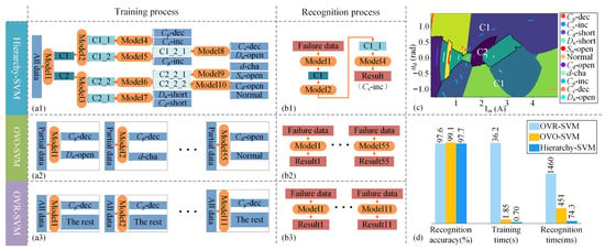
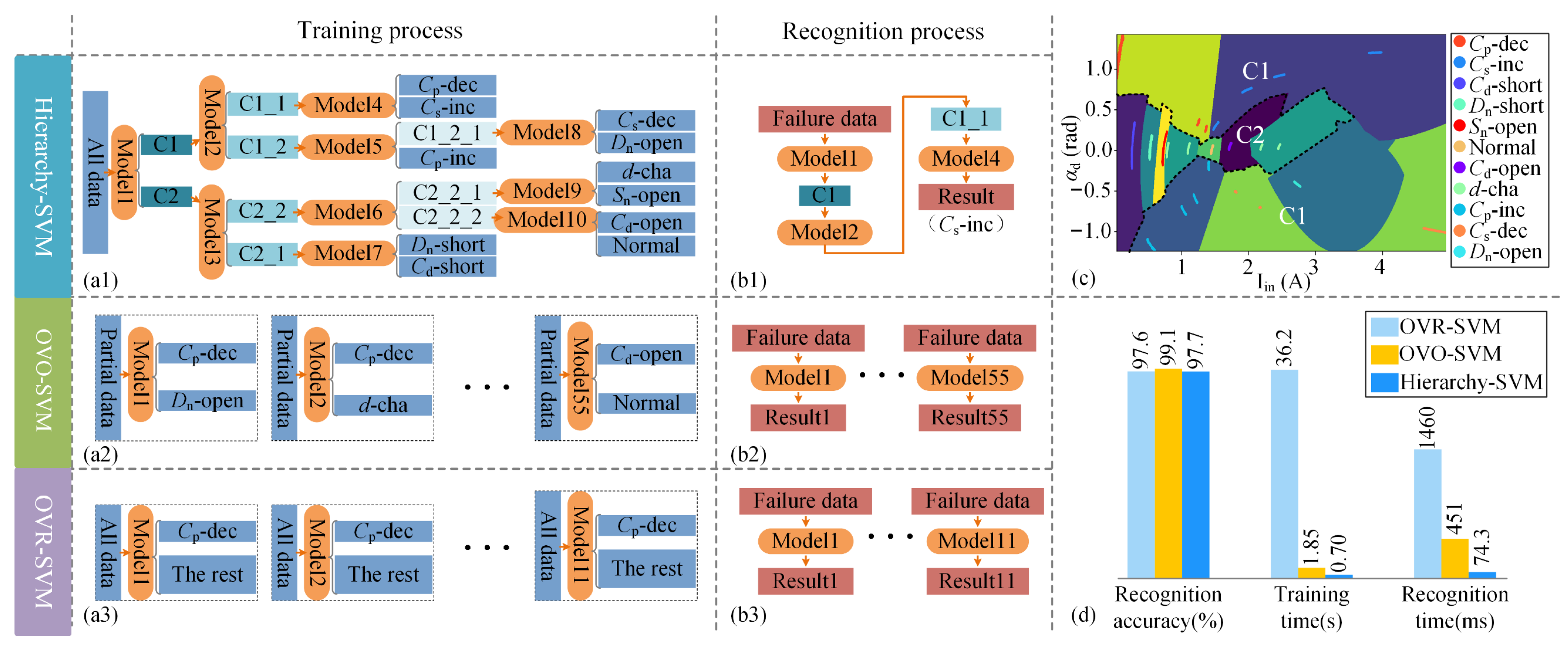
In this paper, n equals 11. The training process of OVO-SVM is as shown in Figure 7(a2). The number of binary SVM models n_o generated during the training process of OVR-SVM equals n, which is shown in Figure 7(a3). Although n_o decreases significantly compared to n_r, every model uses all data to classify one class and the rest, which increases the amount of computation and the number of parameters.

Figure 7. The training process (a1–a3) and recognition process (b1–b3) of Hierarchy-SVM, OVO-SVM, and OVR-SVM; (c) recognition result of Hierarchy-SVM; (d) comparison of recognition accuracy, training time, and recognition time of different strategies.

To improve training and recognition speed, Hierarchy-SVM based on priori knowledge is proposed in this paper. The split of each level is determined based on the physical thresholds analyzed in Section 2 (e.g., distinguishing hard faults from soft faults based on waveform distortion levels), while the specific decision boundaries within each node are learned by the SVM. Based on the priori knowledge of α_d and the amplitude of i_in (I_in), Hierarchy-SVM seeks the distinct separating planes in advance like C1 and C2, divided by the black dotted line in Figure 7c, dividing all the classes into four hierarchies as shown in Figure 7(a1). Within each node k of the hierarchy, a binary SVM is trained to find the optimal separating hyperplane. The decision function at node $k$ is defined as:

$$f_k(x)=sign({\displaystyle \sum _{i\in S{V}_k}{\alpha }_i{y}_{i}K(x_i,x)+b_k})$$

(17)

where SV_k denotes the support vectors selected for node k. The final classification result is obtained by traversing the tree from the root to a leaf node based on the outputs of f_k(x).

To decrease the amount of computation and the number of parameters, the training process of every model uses the same data size by clipped data set. Hierarchy-SVM not only decreases the number of binary SVM models but also simplifies the recognition process. The recognition process OVO-SVM and OVR-SVM both adopt a voting strategy which requires traversing all the models as shown in Figure 7(b2,b3). Hierarchy-SVM only requires traversing four binary SVM models at most to obtain the final result and Figure 7(b1) shows a possible recognition process of it. Through a comparison between Hierarchy-SVM and the two traditional multi-class SVM algorithms on the same collected data set of α_d and I_in, the training time and recognition time show a significant reduction with the similar recognition accuracy. The recognition accuracy and recognition time were evaluated on the independent test set (20% of the total data) that was not used during model training. The specific values are shown in Figure 7d, which reduces training time to 54% and recognition time to 16.5% of those required by the OVO multi-class SVM algorithm. The recognition result of proposed Hierarchy-SVM is displayed in Figure 7c, in which the data points of different classes are divided into different color blocks. It can be seen from Figure 7c that different fault types are divided into different areas, even if the values of the sampling points are discrete like C_p-inc.

To further evaluate the performance of the proposed Hierarchy-SVM, comparative experiments were conducted with three representative machine learning and deep learning models: Random Forest (RF), Artificial Neural Network (ANN), and Convolutional Neural Network (CNN). All baseline models were tuned to achieve accuracy comparable to that of the proposed method. The RF classifier was configured with 20 decision trees to ensure stability. The ANN architecture consists of an input layer matching the feature dimension, two hidden dense layers with 64 and 32 neurons respectively (ReLU activation), and a softmax output layer. A dropout rate of 0.2 was applied to the first hidden layer to mitigate overfitting. The ANN model was trained for 15 training epochs. A lightweight CNN model was constructed for comparison. It includes two convolutional layers (32 and 64 filters, 3 × 3 kernel size) with ReLU activation, followed by max-pooling layers (2 × 2) and dropout (0.25). The feature maps are flattened and passed through a dense layer (128 neurons) before the final classification layer. Specifically for the CNN model, the 2-dimensional feature vector (I_in, α_d) was transformed into a matrix format compatible with convolutional layers, ensuring that the performance difference stems from the model architecture rather than data representation. The CNN model was trained for 10 epochs. The comparison results in terms of Accuracy, Training Time, and Inference Time are summarized in Table 3. To ensure a fair comparison, all baseline models were trained and evaluated using the same dataset described in Section 3.1, where 80% of the data was used for training and 20% for testing. Accuracy is the ratio of correctly classified samples within the independent test set. Inference Time is the total time required to process the entire test set. As shown in Table 3, the proposed method significantly reduces both training and inference times without compromising accuracy.

Table 3. Performance comparison of different fault diagnosis methods.

Method	Accuracy (%)	Training Time (s)	Inference Time (ms)
Hierarchy-SVM (Proposed)	97.7	0.70	74.3
RF	96.5	1.82	158.2
ANN	98.3	25.26	449.4
CNN	97.5	43.26	504.1

4. Experimental Results

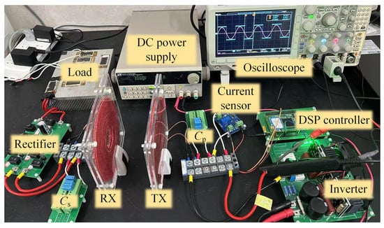
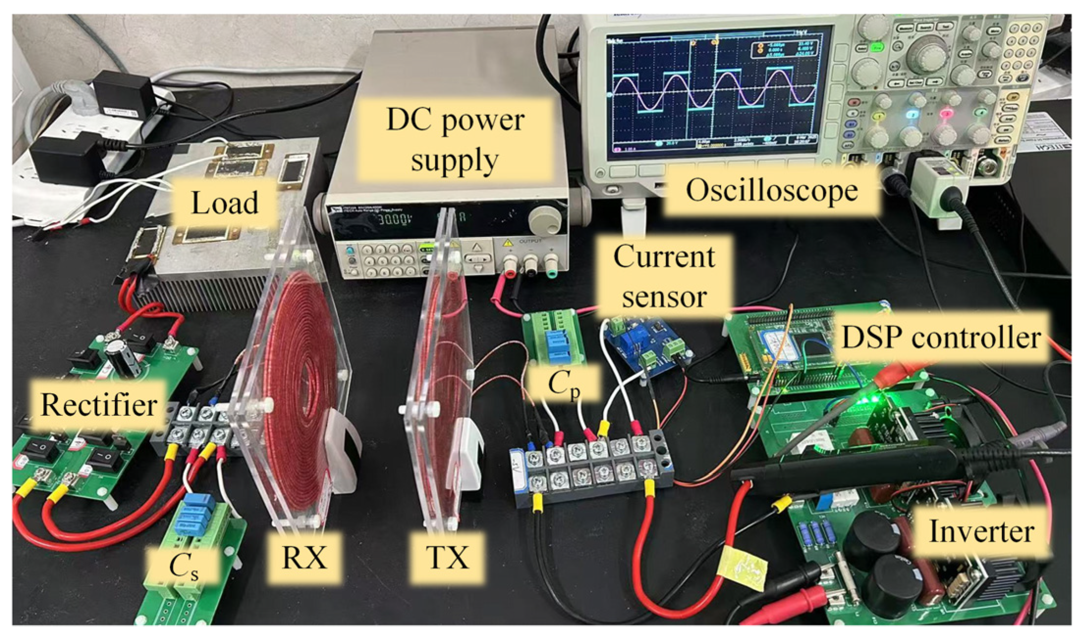
As shown in Figure 8, the experimental prototype is established with the parameter listed in Table 4 to verify the performance of the proposed system-wide fault diagnosis method. Two gallium nitride full-bridge inverters (GSP65R13HB-EVB) are used to generate different frequency PWM signals. The GSP65R13HB-EVB was manufactured by Infineon, headquartered in Hsinchu, Taiwan. A current sensor (LEM CASR 6-NP) is used to measure the value of i_in. The LEM CASR 6-NP current sensor was manufactured by LEM, a company headquartered in Geneva, Switzerland. A microcontroller (TI DSP28377) is used to provide the driving signal for the inverter and collect current data to recognize faults. The TMS320F28377 digital signal processor was manufactured by Texas Instruments, headquartered in Dallas, Texas, USA. The primary side contains a transmitting coil with an S resonant network. The secondary side contains a receiving coil with an S resonant network, a rectifier and a resistor load. All the waveforms are measured using the oscilloscope (Tektronix MDO3024) with differential probes (ETA 5002) and wideband current transducers (Tektronix TCP0020). The Tektronix MDO3024 mixed domain oscilloscope was manufactured by Tektronix, headquartered in Beaverton, Oregon, USA. The ETA 5002 high-voltage differential probe was manufactured by ETA, based in Taipei, Taiwan. The Tektronix TCP0020 current probe was manufactured by Tektronix, headquartered in Beaverton, Oregon, USA.

Figure 8. Photograph of experimental prototype.

Table 4. Parameters of prototype.

Parameter	Value	Parameter	Value
f	100 kHz	Udc	30 V
Lp	349.75 μH	Ls	240 μH
Cp	7.24 nF	Cs	10.55 nF
RL	10 Ω	d	10 cm
RX size	20 cm × 20 cm	TX size	20 cm × 20 cm

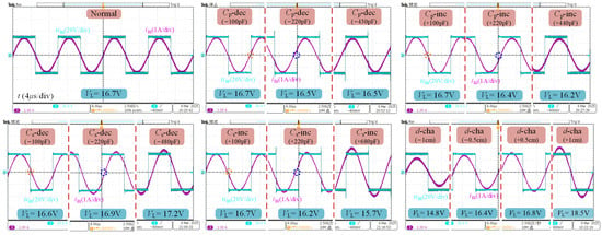
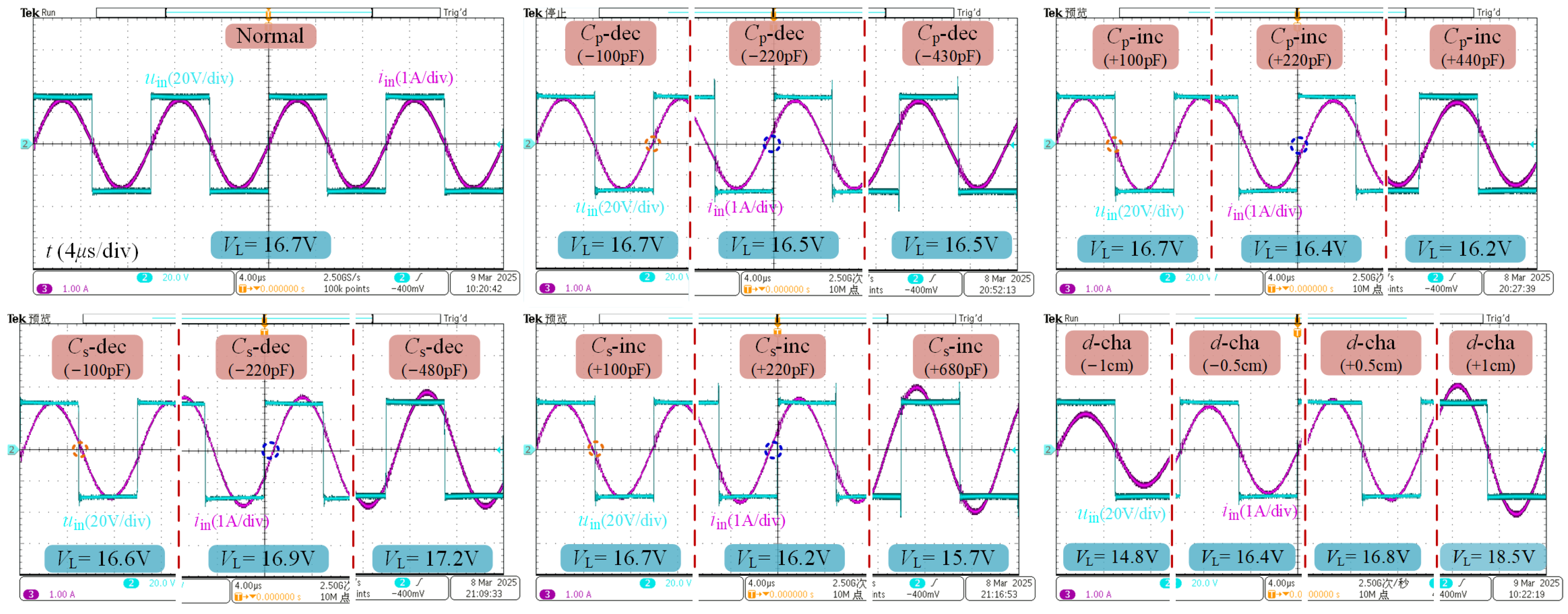
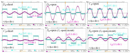
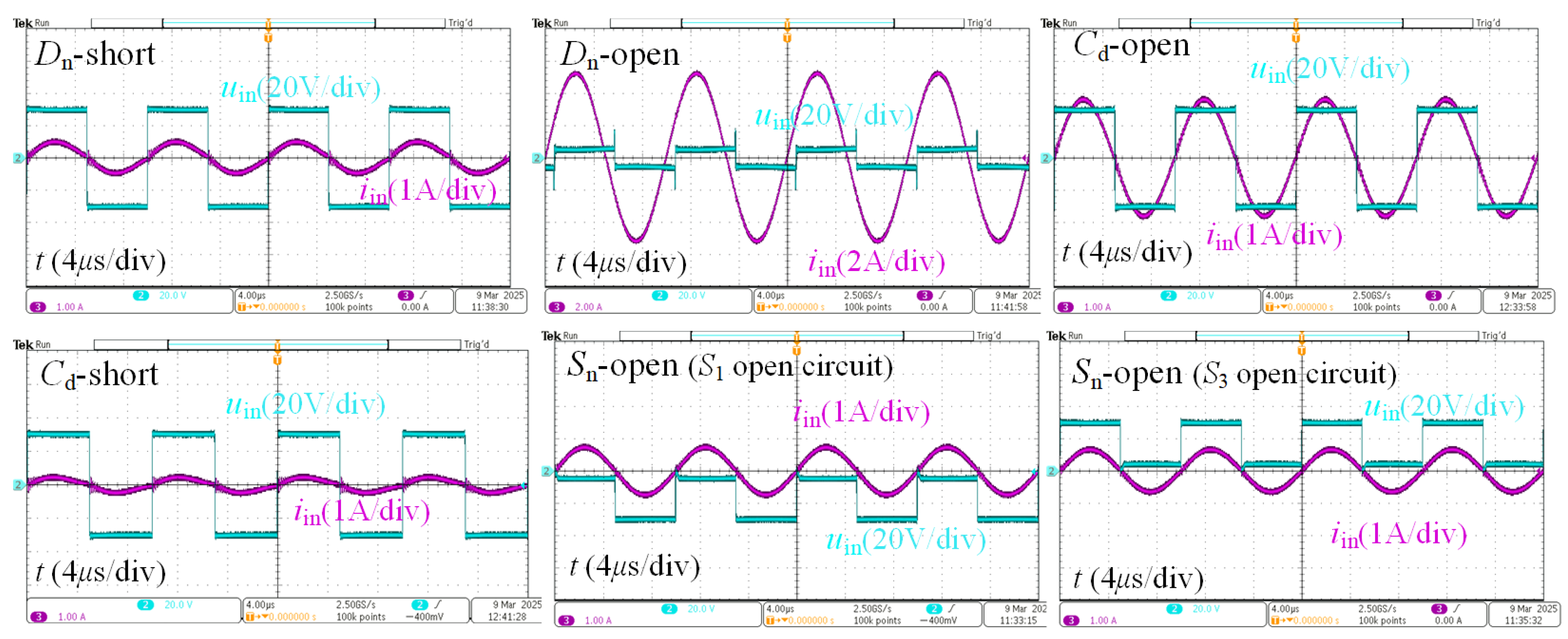
In experiments, the faults caused by parameter drift are called soft faults (including C_p-inc, C_p-dec, C_s-inc, C_s-dec and d-cha) and the faults caused by open-circuit or short-circuit are called hard faults (including S_n-open, D_n-open, D_n-short, C_d-open and C_d-short). The boundary conditions of soft fault diagnosis are derived from the experimental results as shown in Figure 9. It can be seen from Figure 9 that when the capacitor parameter is offset by 100 pF, the load voltage V_L and α_d do not change much. When the capacitor parameter is offset by 220 pF, the α_d has increased significantly which can be obtained by comparing the zero-crossing points of u_in and i_in, which are also circled by a dotted circle in Figure 9. Therefore, 220 pF is selected as the boundary parameter when the capacitor soft faults occur. When the d offsets to 1 cm, V_L fluctuates significantly. Therefore, 1 cm is selected as the boundary parameter of d-cha. The waveforms of hard faults are displayed in Figure 10. The characteristics of i_in and its relationship with u_in are different as shown in Figure 10, which is the basis for diagnosing the class of fault. Under hard faults—such as a switch open-circuit—the topological integrity of the inverter bridge is compromised, which significantly alters the dynamic coupling relationship between the input current and the output AC voltage (i.e., the voltage across the secondary-side resonant tank before rectification). Our method leverages precisely this physical mechanism.

Figure 9. Measured voltage and current waveforms of inverter on normal state and different soft fault states with different offset parameters.

Figure 10. Measured voltage and current waveforms of inverter on different hard fault states.

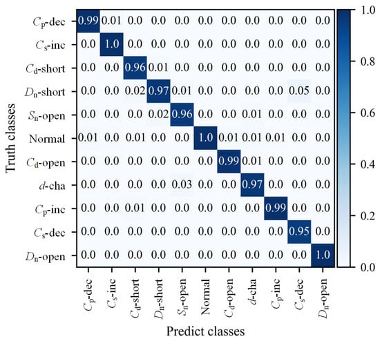
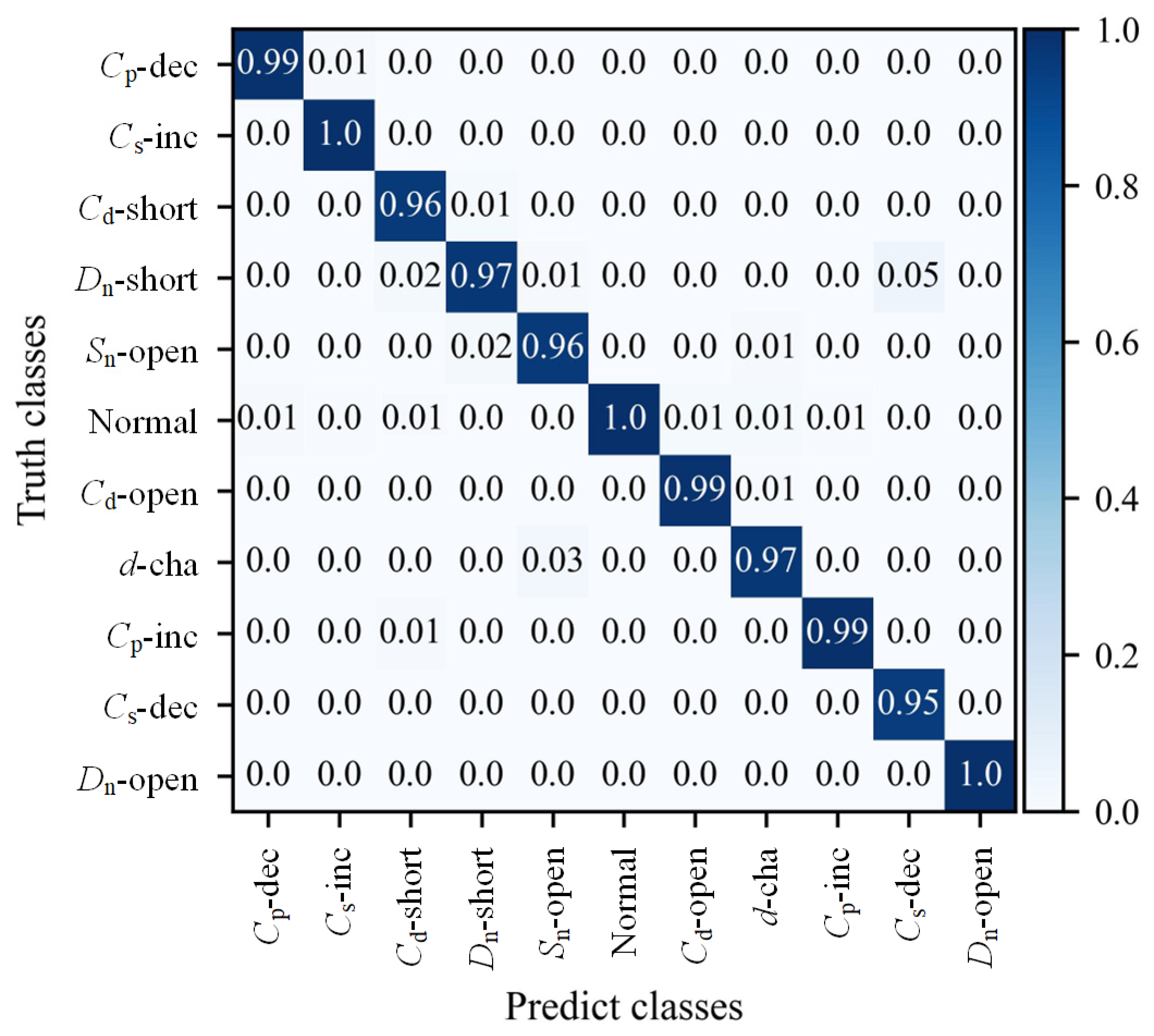
The information of waveforms of i_in on different states is first extracted through a data processing method. This extracted information is then fed into the pre-trained Hierarchy-SVM model, which has been ported to the DSP. The model subsequently outputs the recognition results based on the input data. The confusion matrix of the experiment recognition results is shown in Figure 11. It is observed that most errors occur where normal conditions are identified as soft faults. This phenomenon is attributed to the physical characteristics of soft faults: when the parameter drift is small, the resulting feature signatures are highly similar to the normal operating state, making them difficult to distinguish. This observation is consistent with the boundary condition analysis in Figure 9, where small capacitance offsets (e.g., 100 pF) yielded negligible changes in phase difference. Additionally, other misclassification cases are predominantly found at the interfaces between different fault categories. The recognition accuracy for all categories has reached 95% or higher, which demonstrates the effectiveness and robustness of the proposed method. Table 5 lists the recall rate of different soft faults with different offset parameters in experiments. The specific parameter offset levels for each soft fault are also detailed in Table 5. The recall rate of the model under various offset parameters is 94% or higher. Some of the offset parameters of these tests are not present in the training dataset, but the model can still maintain a high recognition accuracy rate, indicating that the model has good generalization ability.

Figure 11. Confusion matrix of the experiment recognition results.

Table 5. Recall rate of soft faults.

Fault Class	Rate	Fault Class	Rate
Cp-inc (+220 pF)	99%	Cp-dec (−220 pF)	97%
Cp-inc (+440 pF)	98%	Cp-dec (−680 pF)	99%
Cp-inc (+1 nF)	100%	Cp-dec (−1 nF)	100%
Cp-inc (+2.2 nF)	100%	Cp-dec (−2.53 nF)	100%
Cs-inc (+220 pF)	100%	Cs-dec (−220 pF)	95%
Cs-inc (+470 pF)	100%	Cs-dec (−470 pF)	96%
Cs-inc (+1 nF)	100%	Cs-dec (−680 pF)	94%
Cs-inc (+3.3 nF)	100%	Cs-dec (−3.3 nF)	97%
d-cha (+1 cm)	96%	d-cha (−1 cm)	100%
d-cha (+1.5 cm)	96%	d-cha (−1.5 cm)	99%
d-cha (+2 cm)	100%	d-cha (−2 cm)	100%
d-cha (+2.5 cm)	95%	d-cha (−2.5 cm)	98%

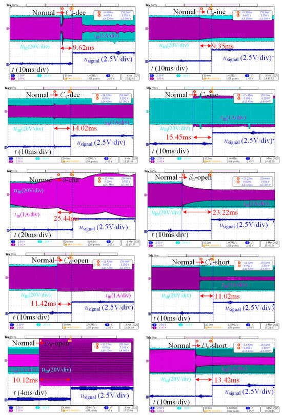
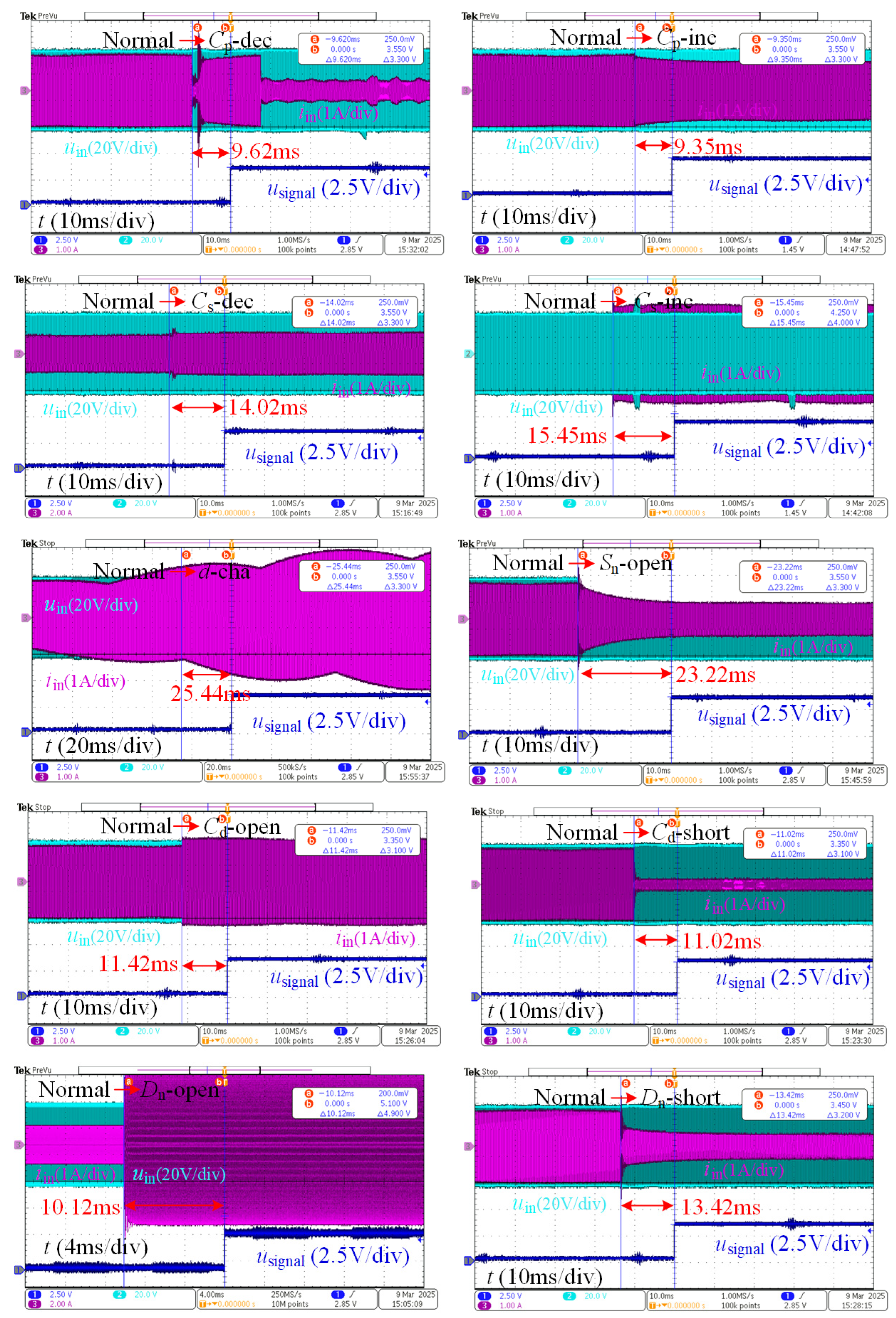
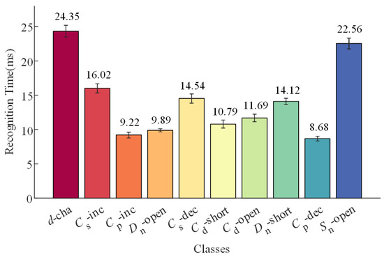
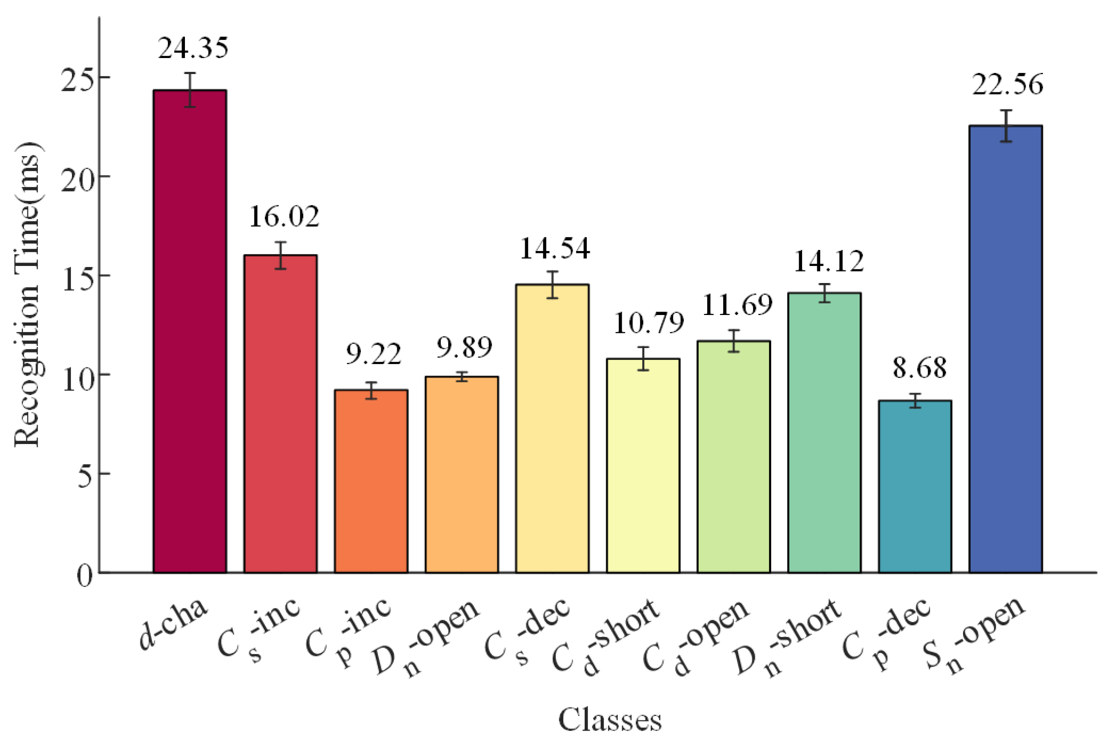
Another critical metric is the recognition speed. To measure the recognition time, the voltage of a DSP pin u_signal is set as the sign of recognition success when its level changes from 0 V to 3.3 V. Then, by measuring the time difference between the occurrence of the fault and the increase in the pin level, the time it takes for the controller to successfully identify the fault can be gained as shown in Figure 12. Figure 12 shows all the waveforms of u_in and i_in and the measurement of the identification time during the transition stage. All faults can be successfully identified in an extremely short time (within 26 ms). The recognition time for each fault category was measured over 10 independent trials. Figure 13 includes error bars representing the standard deviation. The results indicate a mean recognition time of 14.19 ms with a standard deviation of less than 2 ms, demonstrating the high stability and repeatability of the algorithm on the TI DSP28377 controller.

Figure 12. Measured voltage and current waveforms of inverter during the transition stage when different faults occur.

Figure 13. Average results of measured recognition time with standard deviation.

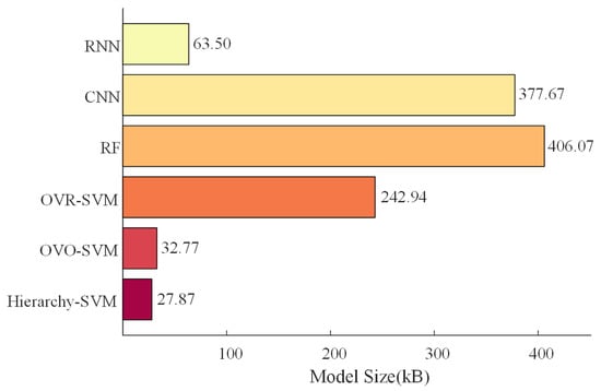
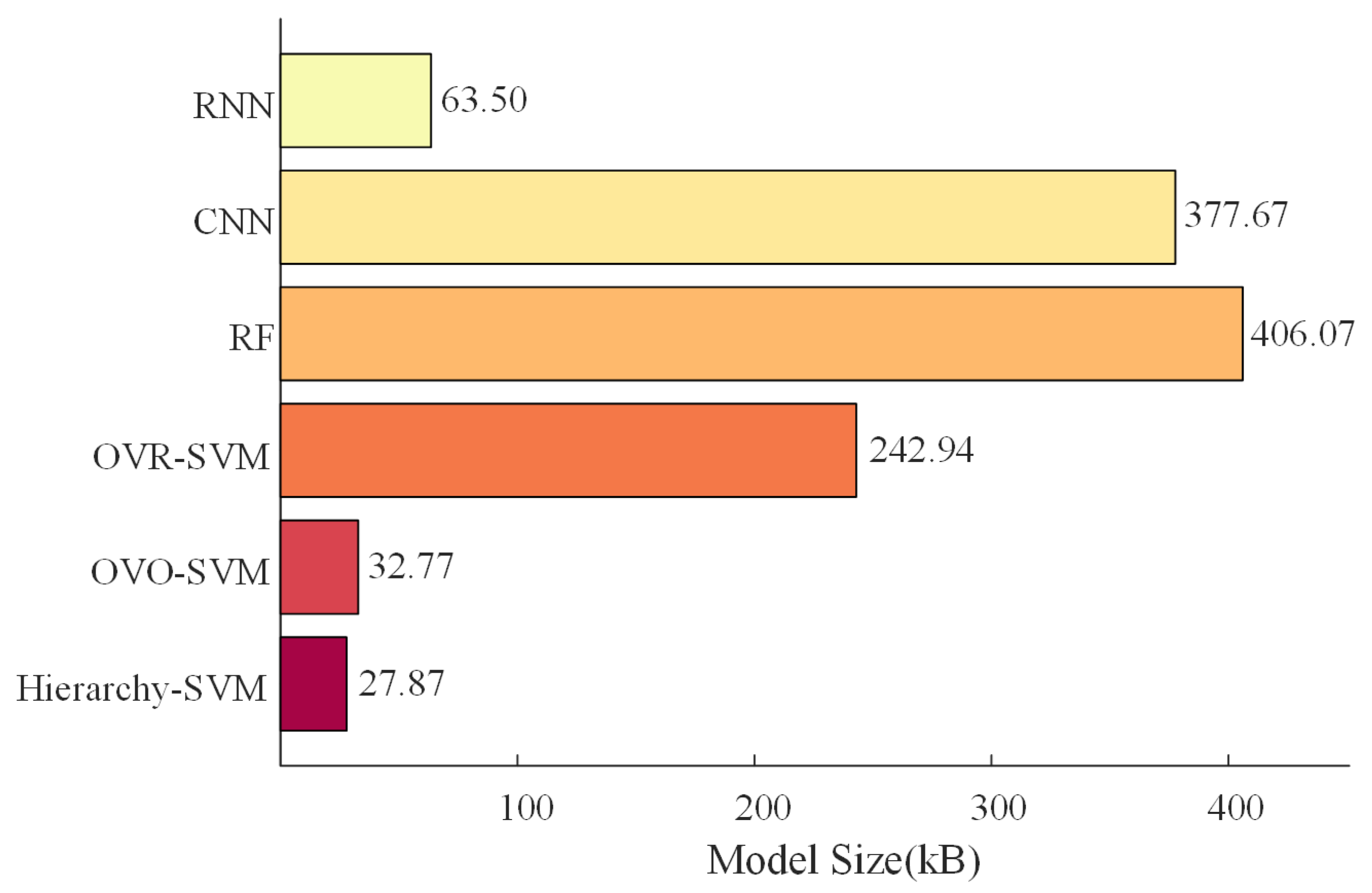
As the trained model needs to be implemented onto the controller which usually has limited storage resources, the size of the model is also very important. As shown in Figure 14, which compares the model sizes of different strategies, the proposed approach achieves a significant reduction in the classification model size. The proposed Hierarchy-SVM strategy reduces the model size by 88.53% compared with OVR-SVM and by 4.9 kB compared with OVO-SVM. Low memory usage improves the applicability of the proposed method on various controllers. Furthermore, the model size can also evaluate the magnitude of the computational load during the identification process. The proposed method not only has a smaller model size than traditional methods, but also only requires partial parameters in the model to participate in the operation during the recognition process as shown in Figure 7(b1), which is another evidence that the Hierarchy-SVM has a faster recognition speed.

Figure 14. The model sizes of different strategies.

Thus, the experimental results show that the proposed fault diagnosis method for WPT systems can effectively identify various faults including all key components in WPT systems. The proposed method achieves a more than 95% accuracy rate in identifying various faults, with a single identification time of average 14.19 ms. Furthermore, the model has a good generalization ability for the different offset parameters of soft faults. In addition, the proposed Hierarchy-SVM has smaller model size and low computational load, demonstrating its practical feasibility and computational efficiency.

5. Conclusions

In this paper, a system-wide fault diagnosis method for WPT systems is proposed and experimentally validated on a prototype, proving the effectiveness of the method. The core innovation of this work lies in the theoretical design of the physics-informed hierarchical structure and the complexity optimization strategy tailored for embedded WPT systems. Unlike conventional hierarchical SVMs that rely on data-driven clustering (e.g., k-means) to determine the tree structure, our Hierarchy-SVM constructs the decision tree based on the physical fault mechanisms of the WPT system. This “Physics-Informed Machine Learning” approach theoretically guarantees better separability for specific WPT faults compared to blind data clustering. The experimental results of the proposed method achieve more than 95% fault identification accuracy with average 14.19 ms recognition time, representing a significant advancement in WPT system diagnostics. The method demonstrates comprehensive diagnostic capabilities across the entire WPT system, featuring several key innovations:

(1)

A meticulously designed Hierarchy-SVM algorithm has reduced both training and recognition times significantly while maintaining high accuracy, enabling practical implementation on conventional system controllers;

(2)

A minimalist hardware configuration requiring only a single current sensor and eliminating the need for primary-secondary side communication, significantly enhancing system applicability.

In practical applications, WPT systems may operate across multiple power levels, experience dynamic coupling variations, or encounter simultaneous multiple faults. Future research will focus on developing adaptive feature extraction techniques and robust multi-task learning frameworks to extend the applicability of this method to dynamic wireless charging scenarios and complex fault conditions.

References

- Liu, W.; Chau, K.; Tian, X.; Wang, H.; Hua, Z. Smart wireless power transfer—Opportunities and challenges. Renew. Sustain. Energy Rev. 2023, 180, 113298. [Google Scholar] [CrossRef] [Scilit]
- Zhang, Z.; Pang, H. Wireless Power Transfer: Principles and Applications; Wiley-IEEE: New York, NY, USA, 2022. [Google Scholar]
- Yin, J.; Mekhilef, S.; Darvish, P.; Mokhlis, H.; Soon, T.K. A New Cross-Overlapped Decoupling Coil Structure for EV Dynamic Inductive Wireless Charging System. IEEE Trans. Ind. Electron. 2025, 72, 1314–1324. [Google Scholar]
- Chen, K.; Zhang, Z. In-flight wireless charging: A promising application-oriented charging technique for drones. IEEE Ind. Electron. Mag. 2023, 18, 6–16. [Google Scholar] [CrossRef] [Scilit]
- Zhao, F.; Jiang, J.; Cui, S.; Zhou, X.; Zhu, C.; Chan, C.C. Research on bipolar non-salient pole transmitter for high-power EV dynamic wireless power transfer system. IEEE Trans. Power Electron. 2021, 37, 2404–2412. [Google Scholar] [CrossRef] [Scilit]
- Wang, F.; Chen, C.; Ye, Z.; Fang, Q.; Yang, G. Magnetically coupled resonant wireless power transmission system: A review of fault diagnosis methods. IEEE Trans. Device Mater. Reliab. 2025, 25, 180–188. [Google Scholar] [CrossRef] [Scilit]
- Dai, X.; Jiang, J.C.; Wu, J.Q. Charging area determining and power enhancement method for multi-excitation unit configuration of wirelessly dynamic charging EV system. IEEE Trans. Ind. Electron. 2018, 66, 4086–4096. [Google Scholar] [CrossRef] [Scilit]
- Jeong, S.Y.; Kwak, H.G.; Jang, G.C.; Choi, S.Y.; Rim, C.T. Dual-purpose nonoverlapping coil sets as metal object and vehicle position detections for wireless stationary EV chargers. IEEE Trans. Power Electron. 2017, 33, 7387–7397. [Google Scholar] [CrossRef] [Scilit]
- Thai, V.X.; Jang, G.C.; Jeong, S.Y.; Park, J.H.; Kim, Y.S.; Rim, C.T. Symmetric sensing coil design for the blind-zone free metal object detection of a stationary wireless electric vehicles charger. IEEE Trans. Power Electron. 2019, 35, 3466–3477. [Google Scholar] [CrossRef] [Scilit]
- Chu, S.Y.; Zan, X.; Avestruz, A.T. Electromagnetic model-based foreign object detection for wireless power transfer. IEEE Trans. Power Electron. 2021, 37, 100–113. [Google Scholar] [CrossRef] [Scilit]
- Low, Z.N.; Casanova, J.J.; Maier, P.H.; Taylor, J.A.; Chinga, R.A.; Lin, J. Method of load/fault detection for loosely coupled planar wireless power transfer system with power delivery tracking. IEEE Trans. Ind. Electron. 2009, 57, 1478–1486. [Google Scholar] [CrossRef] [Scilit]
- Yan, Z.; Zhang, Y.; Zhang, K.; Song, B.; Li, S.; Kan, T.; Mi, C.C. Fault-tolerant wireless power transfer system with a dual-coupled LCC-S topology. IEEE Trans. Veh. Technol. 2019, 68, 11838–11846. [Google Scholar] [CrossRef] [Scilit]
- Han, X.; Hou, Y.; Jiang, C.; Ye, Y. Short circuit fault-tolerant LCC-S wireless power transfer system. J. Power Electron. 2022, 22, 187–197. [Google Scholar] [CrossRef] [Scilit]
- Ayaz, E.; Altun, O.; Polat, H.; Keysan, O. Fault tolerant multi-Tx/multi-Rx inductive power transfer system with a resonator coil. IEEE J. Emerg. Sel. Top. Power Electron. 2022, 11, 1272–1284. [Google Scholar] [CrossRef] [Scilit]
- Li, Y.; Sun, P.; Liang, Y.; Wu, X.; Sun, J.; Rong, E.; Liu, Y.; Deng, Q. Research on rectifier fault diagnosis and self-protecting for inductive power transfer system with constant-current output. IEEE Trans. Power Electron. 2024, 40, 3750–3769. [Google Scholar] [CrossRef] [Scilit]
- Liu, Y.; Zhao, X.; Tian, E.; Sha, Y. Open-circuit fault diagnosis for the inverter of inductive power transfer systems: A rough-set-theory-based method. IEEE Trans. Instrum. Meas. 2024, 73, 1–11. [Google Scholar] [CrossRef] [Scilit]
- Sun, X.; Song, C.; Zhang, Y.; Sha, X.; Diao, N. An open-circuit fault diagnosis algorithm based on signal normalization preprocessing for motor drive inverter. IEEE Trans. Instrum. Meas. 2023, 72, 1–12. [Google Scholar] [CrossRef] [Scilit]
- Li, Z.; Wheeler, P.; Watson, A.; Costabeber, A.; Wang, B.; Ren, Y.; Bai, Z.; Ma, H. A fast diagnosis method for both IGBT faults and current sensor faults in grid-tied three-phase inverters with two current sensors. IEEE Trans. Power Electron. 2019, 35, 5267–5278. [Google Scholar] [CrossRef] [Scilit]
- Xiao, J.; Chen, S.; Fang, X.; Mo, Y.; Liu, Q. Research on Fault Diagnosis Method of Electric Vehicle Dynamic Wireless Power Transfer. In Proceedings of the 2024 10th International Conference on Power Electronics Systems and Applications (PESA), Hong Kong, China, 5–7 June 2024. [Google Scholar]
- Wen, F.; Li, J.; Hao, S.; Yu, G.; Guo, J.; Liu, J. Research on Fault Diagnosis Method for Wireless Power Transfer Systems Based on PSO-SVM. In Proceedings of the 2024 IEEE PES 16th Asia-Pacific Power and Energy Engineering Conference (APPEEC), Nanjing, China, 25–27 October 2024. [Google Scholar]
- Li, C.; Wang, H.; Li, C.; Zhang, Y.; Feng, Y.; Zhang, X.; Negnevitsky, M. Coupled noise-aware uav fault diagnosis based on learnable wavelet packet transform and scale-graph label enhancement. IEEE Internet Things J. 2025, 12, 52913–52926. [Google Scholar] [CrossRef] [Scilit]
- Li, C.; Li, S.; Feng, Y.; Gryllias, K.; Gu, F.; Pecht, M. Small data challenges for intelligent prognostics and health management: A review. Artif. Intell. Rev. 2024, 57, 214. [Google Scholar] [CrossRef] [Scilit]
- Xiao, W.; Huang, X.; Luo, J.; Zhang, B.; Qiu, D.; Chen, Y.; Xie, F. Dynamic Modeling and Control Design Based on Singular Perturbation Theory for High-Order Wireless Power Transfer System. IEEE Trans. Ind. Electron. 2024, 20, 7524–7536. [Google Scholar] [CrossRef] [Scilit]
- Wang, Q.; Huang, R.; Xiong, J.; Yang, J.; Dong, X.; Wu, Y.; Wu, Y.; Lu, T. A survey on fault diagnosis of rotating machinery based on machine learning. Meas. Sci. Technol. 2024, 35, 102001–102011. [Google Scholar] [CrossRef] [Scilit]
- Cortes, C.; Vapnik, V. Support-vector networks. Mach. Learn. 1995, 20, 273–297. [Google Scholar] [CrossRef] [Scilit]
Disclaimer/Publisher’s Note: The statements, opinions and data contained in all publications are solely those of the individual author(s) and contributor(s) and not of MDPI and/or the editor(s). MDPI and/or the editor(s) disclaim responsibility for any injury to people or property resulting from any ideas, methods, instructions or products referred to in the content. |
© 2026 by the authors. Licensee MDPI, Basel, Switzerland. This article is an open access article distributed under the terms and conditions of the Creative Commons Attribution (CC BY) license.