


Abstract
This paper addresses global path planning for a wheeled mobile robot with two different kinematic structures, considering both shortest path and minimum energy consumption criteria. The main research question concerns how the robot’s kinematic structure and the selected planning algorithm influence the resulting path with respect to these criteria. Our review of the state of the art discusses selected path planning methods, including model-based approaches. To determine the energy optimal path, a simplified model of the PIAP GRANITE robot was developed. The robot can be configured as either differentially driven or skid-steered. In the differentially driven configuration, the robot has two driven wheels and two caster wheels, whereas in the skid-steered configuration all wheels are independently driven. The robot’s models are based on previous theoretical and experimental studies and include kinematics, dynamics, drive units, and wheel slip phenomena. For path planning, it was assumed that the robot can move straight or turn. A flat terrain representative of typical urban environments was modeled as a grid of square cells, each characterized by friction and rolling resistance coefficients. Path planning was performed using A*, Theta*, and RRT* algorithms. In order to quantitatively evaluate the results, quality indexes were defined, including path length, energy consumption, computation time, and the number of analyzed nodes. Simulation results are presented for selected terrain maps, both robot configurations, all algorithms, and both optimization criteria. The results show that the differentially driven configuration is consistently more energy-efficient. For the skid-steered robot, minimizing the number of turns is crucial due to high turning energy costs. The A* algorithm consistently finds optimal paths, whereas RRT* is faster but produces non-optimal and non-repeatable results. Theta* does not always achieve optimality due to limitations imposed by the line-of-sight function.
1. Introduction
One of the most common problems in the control of mobile robots is the task of moving from an initial position to a desired final position. This task involves both motion planning and motion execution. Control systems that perform such tasks usually have a hierarchical structure.
Three levels of hierarchy can be distinguished, starting from the highest: global motion planning, local motion planning (also called local navigation), and tracking control or path following. It should be emphasized that, in practice, not all of these levels are always present in a control system, as this depends on the specific application of the robot.
Global path planning is one of the fundamental problems in mobile robotics. The process relies on a map representing the environment, which may include details about the terrain type, surface profile, and obstacles that the robot must avoid. Solving this problem makes it possible to determine the most efficient path from a known initial position to a target destination, while considering obstacles and system constraints, including those specific to the robot. Path planning is formulated as an optimization problem according to a selected criterion, such as minimizing path length, travel time, or energy consumption. The determined optimal path is then provided to the local planner or control system and serves as the basis for further execution of the robot’s motion.
Global path planning is a computationally demanding problem, which necessitates the use of efficient algorithms and is frequently performed offline, i.e., not in real time. The algorithm designed to solve this task should guarantee a solution whenever one exists and, ideally, provide an optimal result. Depending on the robot’s intended application, the algorithm’s execution speed or the proximity of the solution to the true optimum may be the more critical factor. For this reason, it is often advisable to use different algorithms for global path planning depending on the robot’s specific purpose and operational context.
In addition to the choice of algorithm, the robot’s kinematic structure may play a significant role in the path planning process, as the optimal paths can differ depending on the locomotion system, e.g., wheeled, tracked, legged, or hybrid. Even when considering only wheeled robots, various configurations can be distinguished, including both nonholonomic and holonomic systems. For this reason, it is advisable to include the robot model in the path planning process so that the resulting path accounts for the robot’s specific characteristics.
Consequently, this article aims to answer the following key research question:
How do the kinematic structure of the robot and the type of global path planning algorithm influence the planned path, considering both the shortest path and minimum energy consumption criteria?
The answer to this question may be important from the point of view of optimal selection of the algorithm for a given kinematic structure of the robot and the adopted optimality criterion.
Answering this question requires the development of a simulation environment that enables the creation of environmental maps, the formulation of a robot model for the analyzed configurations, the implementation of selected global path planning algorithms, the introduction of quality indexes, and the execution of simulation studies.
The main contributions of this article include the following:
- Development of a simulation environment for global path planning studies, enabling the consideration of various terrain maps, robot kinematic structures, path planning algorithms, and optimality criteria, as well as the presentation of results in the form of quality indexes and motion paths;
- Derivation and implementation of simplified motion models for two kinematic structures, i.e., differentially driven and skid-steered, taking into account kinematics and dynamics aspects, wheel slip phenomena, and drive units characteristics;
- Implementation of selected representative global path planning algorithms for the analyzed robot kinematic structures and optimality criteria;
- Presentation of simulation results for global path planning of mobile robots with different kinematic structures, considering various algorithms, and optimality criteria, including both aggregated results (quality indexes) and detailed results (motion paths and time histories of selected physical quantities);
- Formulation of detailed conclusions from the conducted studies and answers to the key research question concerning the influence of robot kinematic structures and global path planning algorithms on the obtained results for the analyzed optimality criteria.
The novelty and core contributions of this work are related to energy-efficient robot path planning based on a simplified robot model, as well as to the analysis of the influence of both the robot’s kinematic structure and the applied algorithm on the resulting path. Although the algorithms considered in this study are well known in robotics, in the vast majority of existing works the optimization criterion is limited to path length. Moreover, widely available software frameworks typically support only path length optimization. In contrast, this paper explicitly incorporates energy consumption as an optimization criterion.
The contents of the subsequent sections of the paper are as follows:
- Section 2 focuses on a review of the state of the art in the field of mobile robot path planning, taking into account various robot kinematic structures, planning algorithms, and optimality criteria;
- Section 3 presents the research object, the PIAP GRANITE robot, and discusses its model for the two analyzed configurations, including kinematics and dynamics aspects as well as the characteristics of the drive units;
- Section 4 addresses the problem of global path planning for the analyzed robot configurations, including the main assumptions, environmental representation, simplified motion models, optimization criteria and constraints, selected global path planning algorithms used in the study, and the quality indexes adopted for result evaluation;
- Section 5 presents the results of the simulation studies, including the obtained paths, quality indexes, time histories of distance traveled or electrical energy consumption, as well as the conclusions derived from the analysis of individual cases;
- Section 6 provides a summary of the paper, formulates answers to the key research question, and indicates potential directions for future work.
2. State of the Art Review
As indicated in the introduction, the robot’s type of kinematic structure generally affects the result of global path planning. Even when considering only modern wheeled robots, one can encounter configurations such as differentially driven, skid-steered, car-like (Ackermann-steered), rover-type (with a high number of driven and steered wheels), and omnidirectional (Mecanum drive, holonomic drive). Their properties are discussed in Trojnacki & Dąbek, 2019 [1], taking into account mobility, maneuverability, motion stability, dead reckoning, and design complexity.
The state of the art in global path planning algorithms is described, among others, in the book by Bigaj, 2012 [2], as well as in the recent review papers by Sánchez-Ibáñez et al., 2021 [3], Loganathan & Ahmad, 2023 [4], Zhang et al., 2025 [5], Nguyen et al., 2025 [6], and Tang et al., 2025 [7].
These sources indicate that the global path planning problem can be addressed using algorithms belonging to the following categories:
- Classical methods, such as the wavefront method and various potential field method variants, e.g., the work of Hwang & Ahuja, 1992 [8], which enable path planning in simple environments.
- Graph search methods, especially heuristic ones, such as the A* algorithm introduced by Hart et al., 1968 [9], which is the most influential graph search algorithm in robotics and has given rise to many derived algorithms.
- Probabilistic methods, such as Probabilistic Roadmaps (PRM) proposed by Kavraki et al., 1996 [10], and Rapidly-Exploring Random Trees (RRT) presented in Kuffner et al., 2000 [11], as well as their improvements incorporating kinodynamic constraints and adaptive sampling strategies, e.g., the work of Webb & Berg, 2013 [12], and other related algorithms discussed in the survey paper by Zhang et al., 2025 [5].
- Metaheuristic methods, such as genetic algorithms analyzed in Ghorbani et al., 2009 [13], memetic algorithms used in Bigaj, 2012 [2], and ant colony optimization algorithms discussed in Brand et al., 2010 [14].
- Methods based on the dynamic programming principle, employing partial differential equations, such as the Fast Marching Method (FMM) discussed in Chiang et al., 2007 [15].
- Hybrid methods that combine features of the above approaches, e.g., the Hybrid A* algorithm, as presented in works Shamsudin et al., 2017 [16], Kim et al., 2025 [17] and Liu et al., 2024 [18], in which a discretized artificial potential field method is combined with the RRT* algorithm.
Generally, the environment in which a mobile robot operates can be either static or dynamic. Most often, the global path planning problem is solved for a static environment. However, algorithms dedicated to dynamic environments also exist, such as D*, D* Lite, D* Extra Lite, proposed by Przybylski & Putz, 2017 [19], and the method based on Koopman MPC elaborated by Abtahi et al., 2025 [20].
In this paper, further considerations regarding global path planning are limited to the static environment case.
In terms of environmental representation, 2D maps that neglect terrain topography are most frequently employed. Nevertheless, there are works, such as Jaroszek & Trojnacki, 2014 [21], in which variable terrain height is taken into account.
In the context of environmental representation for the robot, discrete metric maps divided into uniform, typically square cells are most commonly used. Paths generated on such maps often include waypoints positioned at the centers of adjacent cells, in which case edge-restricted algorithms are applied, limiting the robot’s movement to a few directions, e.g., eight. Under these conditions, the A* algorithm is commonly applied.
Robot motion can also occur in unrestricted directions, with waypoints placed beyond neighboring cells, by employing any-angle algorithms. If a discrete representation of the environment is used, graph-based methods such as Theta* and Hybrid A* may be utilized in this context.
Path planning can also be performed in continuous space, without dividing the environment into discrete cells. In such a case, sampling-based algorithms may be used, as discussed by Karaman & Frazzoli, 2011 [22], including PRM and RRT (and their extensions PRM* and RRT*), as well as other methods such as genetic algorithms and potential field methods. Solutions based on the A* algorithm are also employed to enable path planning in continuous space, such as the Asymptotically Optimal A* algorithm proposed by Przybylski, 2024 [23].
With regard to the grid resolution of the environment map, it should be noted that high resolution offers greater precision but at a higher computational cost, whereas low resolution increases speed but may oversimplify the environment, missing critical details necessary for safe navigation. The issue of efficient path planning on high-resolution grid maps is addressed in the paper by Zhang & Yang, 2022 [24].
If the objective of global path planning is to determine the shortest path under the nonholonomic constraints of a mobile robot, or if energy consumption is used as the optimization criterion, it becomes necessary to consider a model-based approach. This type of approach to both global and local path planning is examined in Howard et al., 2014 [25]. In contrast, Urvina et al., 2024 [26] proposed an integrated route and path planning strategy that incorporates a traversability model and a motion model of a skid-steered mobile robot. Under such conditions, the kinematics and dynamics aspects of the robot can be incorporated into the planning process. For instance, in the aforementioned work by Przybylski, 2024 [23], the concept of kinodynamic sampling-based planning in a continuous search space was employed. Likewise, Wolek & Woolsey, 2017 [27] discussed model-based path planning for autonomous ground, surface, underwater, and air vehicles, taking into account factors such as the dynamics model, environment representation, objective, and available resources.
In turn, the work by Wu et al., 2024 [28] belongs to the relatively small group of studies that address the issue of mobile robot energy consumption at the global path planning stage. The authors compare the energy efficiency of planned paths in warehouse environments using A*, Dijkstra, and PRM algorithms. In this case, energy consumption is not derived from an explicit analytical energy model of the robot, but is indirectly estimated based on simulations conducted in the Gazebo environment. Another example is the work by Gao et al., 2025 [29], in which deep reinforcement learning techniques are employed. However, energy consumption is not directly derived from the robot’s dynamics model. Deep reinforcement learning is also applied in the study by Yuan et al., 2025 [30], where two Gazebo environments are used for evaluation.
Incorporating the robot’s dynamics and the wheel–ground interaction phenomenon requires the use of knowledge derived from vehicle motion studies. In particular, for motion on paved terrain, the models discussed in Pacejka, 2005 [31] can be used, whereas for motion on unpaved terrain it is necessary to apply models based on terramechanics, whose foundations were formulated by Bekker, 1960 [32]. The requirements for tire models used in the modeling of lightweight mobile robots are addressed in the paper of Dąbek & Trojnacki, 2016 [33].
In the context of global path planning, it is desirable to include the robot’s dynamics model in the simplest possible form.
In order to select an appropriate global path planning algorithm for a given robot, operating environment, and application, the following key characteristics of such algorithms should be taken into account:
- Completeness—the ability of the algorithm to guarantee a solution if one exists;
- Optimality—the ability to guarantee that the solution found is optimal if an optimal solution exists;
- Time Complexity—the computational time needed to obtain a solution, expressed as a function of the number of nodes (for graph-based approaches) or the number of branches (for RRT/RRT*-type algorithms);
- Space Complexity—the amount of memory required to solve the problem, defined analogously to time complexity;
- Environment Representation—indicates whether the algorithm requires a discrete or continuous model of the environment;
- Movement Direction—indicates whether the robot’s motion is edge-restricted (common in discrete representations) or any-angle, meaning motion is allowed in arbitrary directions (typically possible in continuous representations).
Table 1 provides a comparison of selected global path planning algorithms from the previously listed categories, considering the features discussed above. For time complexity and space complexity, the minimal achievable complexity is assumed based on the use of efficient data structures and optimal environment conditions. Furthermore, for graph-based and probabilistic algorithms, the symbol is used consistently to represent the number of graph nodes or the number of samples (tree nodes), respectively.
Table 1.
Comparative overview of selected global path planning algorithms.
The comparative analysis of the selected global path planning algorithms leads to several conclusions, including:
- Not all algorithms are complete; in particular, potential field methods and genetic algorithms are not complete.
- Only some algorithms guarantee finding the optimal solution, namely A* and the Fast Marching Method, as well as RRT* (which is asymptotically optimal), while some provide solutions close to optimal, such as Theta* and Hybrid A*.
- Graph-based algorithms (A* and Theta*) and probabilistic algorithms (RRT and RRT*) exhibit similar time and space complexity; however, they differ in the way the environment is represented.
In practice, the complexity of the A*, Theta*, RRT, and RRT* algorithms may differ significantly. In particular, the A* algorithm can consume much more memory than the RRT* algorithm. The Theta* algorithm may shorten the path, but its visibility checks have variable cost, and their application, especially when minimum energy consumption is the optimization criterion, may not lead to optimal solutions.
If the planned path is intended for direct execution by the control system, then additional important features may include, among others, the smoothness of the generated path or the energy consumption resulting from the robot’s motion model.
Despite these advancements, there is still a lack of comprehensive studies comparing global path planning algorithms across different kinematic models and optimization criteria. While some works have examined path planning for specific robot types, few have systematically evaluated the performance of the same algorithm across multiple kinematic structures. Moreover, the vast majority of publications focus exclusively on shortest path planning.
Therefore, in this paper, a comparative analysis of the A*, Theta*, and RRT* global path planning algorithms is conducted within a common environment and for two popular kinematic structures of mobile robots, namely differentially driven and skid-steered, considering two optimization criteria: the shortest path and the path with minimal energy consumption. For this purpose, a dynamics model of the robot is introduced for both kinematic structures, along with a model of the drive units, which makes it possible to determine the electrical energy required to follow a given path.
3. Models of the Robot
3.1. PIAP GRANITE Robot
This paper focuses on global path planning for a wheeled mobile robot with two selected kinematic structures. To ensure the reliability of the planning process, the simulations are based on a model derived from a real robot. A simplified model of the four-wheeled PIAP GRANITE robot is employed in the study. This robot was developed for research on motion and control systems.
The robot design allows for three different configurations of the locomotion system, i.e.,
- Differentially driven configuration, with two non-steered, driven wheels and two castor wheels;
- Skid-steered configuration, with four non-steered and independently driven wheels;
- Omnidirectional configuration, with four Mecanum wheels.
The issue of global path planning is analyzed for the first two of the above-mentioned configurations. The robot structure for both of these configurations is shown in Figure 1a,b, while Figure 1c,d illustrate the kinematic structures and hypothetical distribution of velocity vectors for these configurations during turning.
Figure 1.
PIAP GRANITE robot and its kinematic structures for configurations: (a,c) differentially driven; (b,d) skid-steered.
It is assumed that the robot moves on a horizontal surface with which a stationary coordinate system is associated. A moving reference frame is associated with the robot, with its origin located at the midpoint of the distance between the centers of the wheels. The geometric centers of individual wheels are marked as . The robot in both analyzed configurations includes mobile platform 0 and wheels 1–4.
Additionally, the following symbols are used: (m)—radius of the driven wheel; (m)—radius of the castor wheel (for differentially driven configuration only); (m)—distance between the front and back centers of wheels; (m)—track width; (rad/s)—angular velocity of spin of the ith wheel.
3.2. Kinematics of the Robot
The robot’s motion typically consists of three phases: acceleration, constant-velocity travel, and braking. However, it is assumed that the distance and time associated with the acceleration and deceleration phases are negligible in relation to the total distance and time of the motion. Similarly, the energy consumption during these phases is a small part of the total energy required for the planned movement. Therefore, for simplicity, the occurrence of acceleration and braking phases is omitted, i.e., the calculations within the planned path are performed as for the movement of the robot at constant velocity.
The following types of robot movements are taken into account:
- Longitudinal motion;
- Turning with a given radius (m).
Transitional phases of motion related to the transition from longitudinal motion to turning and vice versa are omitted.
3.2.1. Experimental Studies of Robot Movement
For both analyzed robot configurations, experimental motion tests were conducted at the PIAP Institute for a variety of predefined trajectories, including longitudinal motion and turning.
The results of these tests for the differentially driven configuration indicate that the slip of the wheels during the robot’s motion can be negligibly small, provided that the desired accelerations of the robot are not too high.
In contrast, the results of experimental motion studies carried out for the skid-steered configuration, presented among others in Trojnacki et al., 2014 [34], show that slip of the wheels always occurs during the robot’s turning and is sufficiently large; therefore, it cannot be neglected. However, during longitudinal motion, slip of the wheels may be neglected if the robot’s linear acceleration is not too high. Thus, in this configuration, slip of the wheels during the robot’s turning must be compensated by appropriately adjusting the desired angular velocities of wheels in order to achieve the desired motion parameters of the robot.
Furthermore, it was observed that during turning or rotation in-place of a skid-steered robot, the current consumed by the drive units is significantly higher compared to longitudinal motion or any motion of the robot in a differentially driven configuration. Figure 2 presents representative results for both configurations of the PIAP GRANITE robot under the same motion scenario, which included longitudinal motion, turning, and longitudinal motion again. Both plots present the values of the current consumed by the robot’s drives, where denotes the index of the drive unit driving the ith wheel, according to the wheel numbering convention illustrated in Figure 1.
Figure 2.
Current consumed by the PIAP GRANITE robot drive units during experimental motion tests for configurations: (a) differentially driven; (b) skid-steered.
For the robot in the differentially driven configuration, Figure 2a shows the current consumption of the drives associated with the driven front wheels 1 and 2, while the currents for the remaining, non-driven wheels are approximately zero, since caster wheels 3 and 4 are used instead of standard wheels (see Figure 1c). In this case, the drive shafts rotated freely without being subjected to any load.
The highest values of the consumed current can be observed for this configuration during the acceleration of the robot, as well as during the change in the desired motion path of the robot’s point from a straight line to a circular arc and vice versa.
For the robot in the skid-steered configuration, Figure 2b shows the current values consumed by the drives of all four driven wheels. In this case, high values of driving torques occur during the robot’s turning due to the substantial resistance generated by the non-steered wheels during their lateral displacement relative to the ground. As a result, this leads to high values of current consumed by the robot’s motors. Furthermore, in this configuration, excessive lateral forces during the robot’s turning can result in wheel damage or even detachment from the robot’s body. In turn, during the acceleration of the robot, the maximum current values consumed by the individual wheels are slightly lower than in the differentially driven configuration, since the drive is distributed across all four wheels.
Other studies such as Effati & Skonieczny, 2023 [35], as well as Guo et al., 2019 [36], also indicate that skid-steered robots exhibit significantly higher energy consumption during rotation in place or turning maneuvers compared to straight-line motion.
Taking into account the results of the presented experimental studies, as well as conclusions drawn from other research works, both slip of the wheels and the high current consumed by the robot’s drive units should be taken into account in the motion planning process for skid-steered configuration, while the number of turns should be kept to a minimum.
3.2.2. Velocities in Longitudinal Motion
It is assumed that during longitudinal movement for both configurations, the robot’s wheels roll without slip; therefore, the following relationships are satisfied
where (m/s) is the longitudinal velocity of the geometric center of the ith wheel and (m) is the radius of that wheel.
3.2.3. Velocities During Turning
It is assumed that during the robot’s turning with radius (m), the following relationships occur between the linear velocity (m/s) of the robot’s point and the angular velocity (rad/s) of turning of the mobile platform:
The convention used in this paper assumes that the turning radius (m) is positive for left-hand turns and negative for right-hand turns; therefore, its sign matches the sign of the angular velocity (rad/s).
Instead of the turning radius (m), one can also use its inverse, i.e., the curvature.
Moreover, during turning, the distribution of velocity vectors at characteristic points for both robot configurations reveals the following dependencies:
The above relations concerning the velocities of the geometric centers of the front driven wheels also apply to the robot in a skid-steered configuration, for the corresponding rear wheels.
In the case of a differentially driven robot configuration, due to the negligible slip of the wheels when turning, it can be assumed that the following relations are satisfied:
The motion parameters of castor wheels 3 and 4 are not important from the path planning point of view.
In the case of a robot in a skid-steered configuration, due to slip of wheels occurring when turning, it is assumed that the following relations hold:
where (m/s) and (m/s) are components of the slip velocity, that is, the velocity of motion of points of the wheel which are in contact with the ground with respect to the ground while (m).
The results of experimental studies of the PIAP GRANITE robot’s motion for the skid-steered configuration showed that during turning the absolute value of the slip velocity (m/s) can even be equal to half of the value of the wheel circumferential velocity (m/s) and close to the value of the velocity (m/s). This means that the value of the longitudinal slip factor can reach 50% in this case.
Taking this into account, it is assumed in simplification that for this robot configuration the slip of the wheels during turning is constant, and the value of the longitudinal slip factor is λ = 50%. Therefore, the following relations apply:
As indicated by the results of simulation studies presented in Trojnacki, 2025 [37], the compensation of the slip of the wheels at the stage of controlling the robot’s wheels allows us to obtain values of the robot’s generalized velocities (m/s) and (rad/s) close to the desired ones.
3.2.4. Distance and Time of Movement
In steady motion with velocity (m/s), the following relations hold between the distance (m) and the time of motion (s):
When turning with constant angular velocity (rad/s), the following dependencies occur
where (rad) is the change in the robot’s course.
The case of turning with variable velocity is omitted because, as mentioned earlier, it is assumed that the velocity change occurs only in the longitudinal motion.
However, it can be noticed that when turning, the relationship between the distance (m), the change of course (rad), and the turning radius (m) is:
As a reminder, according to the adopted convention, the turning radius (m) is considered positive for left turns and negative for right turns.
3.3. Dynamics of the Robot
Energy-efficient global path planning requires the inclusion of a robot dynamics model for both analyzed configurations.
It is assumed that in the general case of robot motion, the following relations for the components of the linear acceleration of the robot’s center of mass are satisfied:
Therefore, from Newton’s second law of dynamics it follows that in the steady motion of the robot, i.e., with longitudinal acceleration equal to zero, the sum of the longitudinal forces acting on the robot is also equal to zero, i.e., the following relationship is satisfied:
The normal components of the ground reaction forces for robot’s wheels can be determined from the relationship proposed in the paper of Trojnacki, 2025 [37]:
where and .
The tangential components of the ground reaction forces depend on the robot configuration and the type of motion.
The rotational dynamics of the wheels can be described by the following equation:
where (kg·m2) is a mass moment of inertia of the ith wheel relative to its axis of rotation, (Nm) is the driving torque, (–) is a coefficient of rolling resistance, and (rad/s) and (rad/s2) are the angular velocity and acceleration of this wheel, respectively.
Since this study considers only the case of the robot’s motion with a constant linear velocity, the influence of the wheels’ mass moments of inertia (kg·m2) on the motion will be neglected. These inertia effects impact the robot’s motion during transitional phases between longitudinal motion and turning (and vice versa), but their significance is minor compared to the influence of the forces resulting from wheel–ground interaction.
Based on Equation (15) and assuming that , the driving torques (Nm) can be determined (inverse dynamics problem):
3.3.1. Dynamics of Robot’s Longitudinal Motion
Assuming that the robot moves without slip of the wheels and at a constant velocity, for the differentially driven configuration, based on the Equations (13) and (16) one obtain
where the subscripts and denote the wheels at the front and back of the robot, respectively.
In turn, for the skid-steered configuration, we can use the following formulas:
3.3.2. Dynamics of Robot’s Turning
For the differentially driven configuration, assuming the robot moves without slip of the wheels and with constant velocity, and neglecting the phases of change in the angular velocity of the turn, one can use similar relations as for the longitudinal motion. In this case, however, the influence of the normal component of the linear acceleration of the center of mass on the robot dynamics must be additionally taken into account.
Therefore, these relationships have the form:
For the skid-steered configuration, the longitudinal forces can be determined, for example, based on the Kiencke tire model described in the book by Kiencke & Nielsen, 2005 [38], which takes into account the occurrence of wheel slip. In this case, the influence of the normal component of the linear acceleration of the robot’s center of mass can also be taken into account.
The values of longitudinal forces are then determined using the relationship
where (–) is a friction scaling factor, which denotes the value of longitudinal slip corresponding to the value of maximum tire adhesion coefficient (–).
In turn, the driving torques can be calculated using the equations:
It can be seen that determining the lateral components of the ground reaction forces is not necessary for further analysis. Moreover, it is assumed that the tangential component of the ground reaction forces does not exceed the value of the friction force developed during the entire robot motion.
3.4. Model of the Robot Drive Units
The analyzed robot is equipped with drive units that allow independent control of each wheel. Each drive unit consists of an identical DC motor, encoder, and gear system. The maximum motor input voltage for drive units is (V), which corresponds to the maximum motor rotational speed (rpm) and the resulting maximum angular velocity of wheel (rad/s).
The model of the drive units can be used to determine the values of the rotor current (A) and the motor voltage inputs (V) necessary for the assumed robot motion, based on the known driving torques (Nm).
Neglecting variations in the angular velocities of the wheels during the robot’s motion, the following relations can be used
where (A) is the rotor current, (Ω) is the resistance of the rotor, (Vs/rad) is an electromotive force constant, (Nm/A) is a motor torque coefficient, and (–) and (–) are the gear ratio and efficiency factor of the transmission system, respectively.
For evaluating the electrical energy demand and potential optimization of energy efficiency, it is possible to calculate the electrical power (W) necessary to rotate the ith wheel with the angular velocity (rad/s) and to generate the driving torque (Nm) for that wheel by the drive unit. Knowing the input voltage (V) and the rotor current (A), the absolute electrical power (W) can be determined from the formula:
In addition, the electrical power (W) consumed by other robot systems must be taken into account. Therefore, the total electrical power consumed by the robot can be calculated from the relationship:
In turn, the mechanical power for the robot’s drive units can be calculated based on the following relationships:
Knowing the mechanical power for the drives and the electrical power for the entire robot, one can calculate the electrical and mechanical energy, i.e., (J) and (J), respectively, using the formulas
where (s) denotes the duration of the robot’s motion along the analyzed path.
4. Global Path Planning of a Mobile Robot
4.1. General Assumptions
Path planning of a mobile robot is carried out under the following assumptions:
- The terrain on which the robot moves is flat and typical of an urbanized area; therefore, a two-dimensional representation of the environment is introduced.
- The robot moves at a constant velocity from a known starting position to a desired final position.
- The robot moves straight forward or turns with a radius that depends on the change in the direction of movement.
- The subjects of path planning are the two previously discussed configurations of the PIAP GRANITE robot.
- During path planning, the previously developed robot models are applied, considering the dependencies arising from the kinematics and dynamics aspects, as well as the characteristics of the drive units.
- In the robot path planning process, two optimality criteria are considered: path length and energy efficiency.
- In order to determine the path for the selected optimization criterion, algorithms belonging to different classes are used, i.e., A*, Theta* and RRT*.
- The results for individual cases are compared using quality indexes, allowing for an objective assessment of individual cases.
- A unified grid-based environmental representation is employed for all algorithms.
The selection of A*, Theta*, and RRT* algorithms for the presented study was made to represent three major classes of global path planning approaches: heuristic graph search, any-angle search, and probabilistic sampling-based planning. These algorithms were chosen due to their complementary characteristics, which allow a systematic comparison across different robot’s kinematic structures and optimization criteria, while keeping the computational and implementation complexity manageable. More complex methods, such as Hybrid A* or multi-objective planners, were excluded to maintain comparability and focus on the effects of path length and energy consumption for the considered robot’s kinematic structures.
4.2. Environment Representation
The environment is represented as a metric map divided into equal square cells with a side length (m), exceeding the robot’s maximum dimensions. A stationary reference system is associated with the environment, in which the robots’ motion is described, including their paths.
Individual map cells can represent different types of terrain, with specific properties, as well as obstacles that the robot cannot overcome. The terrain on which the robot can move is characterized by adhesion coefficients and rolling resistance , resulting from tire–ground interactions.
It is assumed that the robot initially occupies the center of the starting cell and the robot ends its movement in the central part of the final cell. Moreover, in the initial position the robot has an orientation that results from the movement to the next cell, i.e., there is no need to rotate it.
Path planning consists in determining the motion path associated with the movement of the robot’s point through a given cell. If the robot’s direction of motion does not change, point moves in a straight line. If the robot changes its direction of motion, the planned path for point consists of a circular arc with radius (m) and may also include a straight-line segment, as illustrated in Figure 3, which shows a change in the robot’s heading by an angle . A positive value of the angle (rad) indicates that the robot turns left (rotation in the direction of the robot’s -axis), whereas a negative value indicates a right turn.
Figure 3.
Path planning of the robot in the case of a change in the direction of motion.
Figure 3 illustrates successive positions of the robot’s point , denoted as , where . The depicted path of point marked in blue consists of a straight-line segment of length (m), followed by a circular arc between points and with radius (m) and length (m) and finally a straight-line segment of length (m). It can be observed that as the value of the angle (rad) decreases, the difference between the length of the path and the length of the path composed of straight-line segments and also decreases.
In the case of the A* algorithm, it is assumed that the robot can move to eight neighboring map cells. Therefore, during movement between cells, the robot’s course can change by the value (rad), where .
Here, the turning radius is determined by the robot’s change in direction (rad) and the grid cell size (m), according to the following equation:
For the Theta* and RRT* algorithms, which belong to the category of any-angle algorithms, the change in the robot’s direction of motion (rad) can take any value and results from the relative positioning of waypoints on the map, with their locations rounded to the centers of the cells, which in this case do not have to be directly adjacent. The turning radius in these cases is determined in an analogous manner.
4.3. Robot Constraints
The robot constraints that can be considered during path planning include:
- Maximum linear and angular velocities and accelerations—for simplicity, the robot is assumed to move with a constant linear velocity (m/s), which can be maintained along the entire path, and the turning radius (m) is assumed to be sufficiently large to allow motion with the desired angular velocity (rad/s) as well as the angular velocities of the wheels (rad/s);
- Tangential and normal forces—it is assumed that the terrain is flat and that slip of wheels does not occur during the robot’s longitudinal motion;
- Maximum driving torques, along with the maximum current and electrical power of the drives—the limitations are based on catalog data and the drive units model;
- Maximum current and electrical power, as well as battery capacity—these limitations are neglected in this paper.
The assumption of robot motion at a constant linear velocity is reasonable for global path planning, as it has minimal impact on total energy consumption. This is because changes in linear velocity occur only briefly at the beginning and end of the motion path. However, angular accelerations arising during direction changes can locally increase energy usage. To mitigate this effect, smoother transitions between straight-line and turning motion could be implemented during trajectory execution, for example using curvature-continuous transition curves (e.g., clothoids). Furthermore, in practical implementations, energy lost during wheel acceleration can be partially recovered during braking, further reducing the influence of both linear and angular accelerations on overall energy consumption.
4.4. A* Algorithm
The A* algorithm belongs to the algorithms of informed graph search and has wide applications in robotics and artificial intelligence. This algorithm can be used in particular for the global path planning of vehicles, taking into account various optimality criteria, where the map of the environment has a representation in the form of a graph.
The A* algorithm assumptions were originally formulated by Hart et al., 1968 [9]. Thanks to the inclusion of admissible heuristics, the algorithm can find an optimal path in a shorter time compared to the use of uninformed algorithms, such as Dijkstra’s algorithm, developed in 1956. In practice, the complexity of the A* algorithm depends on the chosen heuristic function.
The operation of the algorithm is based on the evaluation function in the form
where is the cost associated with the movement from the initial node to node , and is a heuristic function that roughly estimates the cost of motion from the current node to the destination node .
Each node , , corresponds to a map cell whose center has coordinates and . As a result of the algorithm, a path is obtained.
The cost of motion in the above-described evaluation function depends on the adopted optimality criterion, which in this work is either the minimization of path length or energy consumption. In both cases, it is crucial that the adopted heuristic is admissible, i.e., that it does not overestimate the actual cost associated with the movement to the destination node .
In the case of path length optimization it is assumed that
where (m) is the distance covered by point of the robot (path length) while moving in node , that is between nodes and in time (s), where .
The path traveled by the robot’s point in the initial and final map cell, i.e., and , respectively, takes into account the movement of this point between the center of this cell and the boundary of this cell with the previous or next cell (see Figure 3).
The evaluation function allows us to determine the length of the path as the sum of the path covered by the robot’s point from the initial node to the current node and the minimal length of the remaining path as the distance from the current node to the final node , i.e., the Euclidean distance (m). The adopted heuristic is therefore admissible, because it corresponds to the shortest possible path leading from the current node to the destination node in the shortest possible time equal to (s).
In the case of optimization of energy consumption by the robot, it is assumed that:
The energy (J) is associated with the robot motion in node , i.e., between nodes and at time (s).
Since the path is drawn between the centers of the cells, the total energy is calculated as the sum of the energies for particular cells, which depend on the type of terrain in cells.
4.5. Theta* Algorithm
The Theta* algorithm is part of the family of informed search methods and represents an improvement and generalization of the traditional A* algorithm. Introduced in the paper of Daniel et al., 2010 [39], the Theta* algorithm allows any-angle path planning, enabling the generation of smoother and often shorter trajectories compared to the grid-constrained paths obtained by the standard A* algorithm.
The primary innovation of the Theta* algorithm lies in the explicit consideration of line-of-sight conditions when determining optimal parent nodes during node expansions. Unlike the A* algorithm, which restricts movement to adjacent grid nodes, the Theta* algorithm directly connects nodes if an unobstructed straight-line path exists between them, effectively bypassing intermediate grid nodes and reducing unnecessary directional changes.
The evaluation function used in the Theta* algorithm remains analogous to that of the A* algorithm (see dependency (36)). Therefore, the heuristic and cost functions follow the same equations presented earlier in the description of the A* algorithm, that is (37) and (38) for the shortest path criterion as well as (39) and (40) if the energy-efficient criterion is applied.
This approach leads to paths comprising straight-line segments whenever possible, producing smoother and more realistic trajectories suitable for robotic navigation. However, it is still assumed that the nodes from which the path is built are limited to the centers of the map cells.
4.6. RRT Algorithm
The RRT* algorithm was elaborated within the paper of Karaman & Frazzoli, 2011 [22]. RRT* is a probabilistic incremental path planning algorithm that randomly generates a real-time exploration graph called a tree. It is an improved version of the RRT algorithm described in Kuffner & LaValle, 2000 [11], in which the algorithm rebuilds the tree to optimize the path. The RRT* algorithm combines efficient exploration of the state space with asymptotic convergence to an optimal solution. The time complexity of both algorithms is , and the space complexity is , where is the number of samples.
Unlike the A* algorithm, which systematically explores all possibilities, the RRT* algorithm randomly samples points in the search space and connects them to the existing tree in a way that minimizes the cost of reaching a given node. It is a stochastic algorithm, so the path planning results differ between runs. This algorithm does not require dividing the environment into identical cells, but it is possible to limit the path planning to the centers of cells, so that the results can be easily compared with those obtained for the A* algorithm.
In order to compare the path planning results of the A* and RRT* algorithms, it is assumed that the sampled points in the map space are rounded to the centers of the cells. Then, as before, the exact path is calculated, taking into account the radii of the turns.
Then, a point in the map space obtained as a result of the RRT* algorithm can be defined analogously to the A* algorithm, i.e., in the form: , . Similarly as before, the algorithm produces a path (more precisely, a search tree) that can be written as .
The operation of the algorithm for each iteration is as follows:
- Sampling: A random configuration is sampled from the configuration space (taking into account rounding to the center of the nearest map cell).
- Nearest Neighbor: The nearest node in the existing tree to is identified.
- Steering: A new node is generated by steering from node towards node , taking into account environmental constraints and obstacle avoidance.
- Near Nodes: A set of nodes is determined near node , with a radius depending on the number of nodes in the tree , which is defined as , where is a constant parameter that determines the size of the sampling area.
- Choose Parent: Selecting the best node from the set that minimizes the total cost to reach node , i.e.,where is the cost of traveling to node , and is the cost of local motion from node to node .
- Add New Node: Adding node to the tree with parent .
- Rewiring: Checking for each node , whether the connection through provides a lower cost. If , then update the parent of node to node , and propagate the cost changes to its descendants if necessary.
The number of algorithm iterations can be predefined or determined based on an additional convergence condition toward the optimal value. In particular, it can be assumed that the condition for terminating the algorithm can be the percentage difference in the cost of the determined path for the current and previous iteration. For this purpose, an additional parameter (–) is introduced, which determines whether the algorithm may be terminated earlier.
The cost in the case of the RRT* algorithm for cell of the map is calculated in the same way as the function for the A* algorithm—see Formulas (37) and (39).
Similarly to the Theta* algorithm, the RRT* algorithm employs line-of-sight checking, allowing direct connections between nodes without intermediate ones if unobstructed straight paths exist.
5. Simulation Studies
5.1. Robot and Its Environment
In the simulation studies, the previously described models of the PIAP GRANITE robot were used for both the differentially driven and skid-steered configurations. These models take into account the robot’s dynamics and the characteristics of its drive units.
The basic parameters of the robot used in the simulation studies are summarized in Table 2. These parameters include the robot’s dimensions, component masses, and center-of-mass coordinates, as well as the parameters of the integrated Maxon drive units, which consist of DC motors, planetary gears, and optical encoders.
Table 2.
Basic parameters of the PIAP GRANITE robot adopted for simulation studies.
For the simulation studies, the robot’s steady motion velocity was set to .
In the simulation studies, maps typical of urban areas were analyzed. In this work, each map cell is assumed to represent terrain that is traversable by the robot, including surfaces such as concrete, rolled gravel, unpaved road, and field, as well as areas inaccessible to the robot, which may include buildings, elevations, depressions, and water reservoirs. Each square map cell is assumed to have a size of , corresponding to an area of of terrain.
The coefficients adopted in the simulation studies to characterize the tire–ground interaction for the analyzed types of traversable terrain are shown in Table 3.
Table 3.
Tire–ground contact parameters adopted for simulation studies.
These coefficients appear in the previously described models of robot dynamics. Moreover, for the skid-steered configuration, a friction scaling factor of % is applied, along with a constant longitudinal slip ratio during turning of λ = 50%.
5.2. Quality Indexes
To quantitatively evaluate the results for individual global path planning algorithms and robot kinematic structures, the following quality indexes were adopted:
- Path Length (m)—total distance traveled by point of the robot from the starting position to the final one, including all straight-line segments and circular arcs;
- Electrical Energy Consumption (J)—total electrical energy consumed by the robot’s drive units and onboard electronics along the analyzed path;
- Computation Time (s)—algorithm runtime for generating the final path;
- Number of Nodes (–)—number of nodes explored or sampled by the algorithm, representing search efficiency.
These quality indexes are evaluated independently of the selected optimization criterion (shortest path or minimum electrical energy consumption). This will make it possible, for example, to compare how changing the optimization criterion affects the robot’s electrical energy consumption.
5.3. Research Environment and Methodology
Dedicated software was developed for the simulation studies that enables the creation of terrain maps and incorporates the selected global path planning algorithms, robot models for the analyzed kinematic structures, and computations of the previously described quality indexes.
Regarding the research methodology, separate studies were carried out for both analyzed optimization criteria, i.e., the shortest path and minimum energy consumption, on various terrain maps. In each case, for a given terrain map, both robot kinematic structures (differentially driven and skid-steered) were analyzed, along with the individual algorithms, namely A*, Theta*, and RRT*. In all cases, the results are presented in the form of paths and quality indexes. For the RRT* algorithm, the influence of the parameters and on the results was additionally analyzed, particularly regarding their convergence toward the optimal solution. Furthermore, a limitation on the maximum number of algorithm iterations was introduced.
5.4. Results of the Simulation Studies
Based on the research conducted to determine the optimal parameter settings for the RRT* algorithm, it was found that the best performance is achieved for and , with the maximum number of iterations set to . In certain cases, however, even is required to obtain results approaching the optimal solution.
Increasing the parameter in the RRT* algorithm causes the tree to explore the space more extensively in search of better paths. However, this comes at the cost of increased computational effort in each iteration. Therefore, it is reasonable to search for the optimal value of the parameter. It was also observed that the parameter has a marginal impact on path quality once exceeds the threshold value .
Figure 4 illustrates the legend describing path designations for the various robots and algorithms, together with the legend indicating the terrain types present on the analyzed map. It also presents the simulation results for both robot kinematic configurations, the Mixed City Landscape Map and under the shortest path optimization criterion. On all maps the initial position of the robot is marked in orange and the target position in yellow.
Figure 4.
Results of the simulation studies for the Mixed City Landscape Map and the shortest path optimization criterion for the following cases: (a) A* algorithm; (b) Theta* algorithm; (c,d) RRT* algorithm for , , and , , , respectively.
According to the legend, the paths for the respective results are illustrated using different colors. With regard to the path illustrations, the graphs display straight-line connections between the points, whereas the calculations are based on smooth paths that include turning arcs, following the computation methodology described earlier (see Figure 3).
Since energy consumption is not considered by the algorithms, the obtained paths are identical for both kinematic structures for the A* and Theta* algorithms. This is attributed to the use of the cost function independent of the kinematic structure of the robot.
In the case of the RRT* algorithm, depending on the selected parameters, the obtained results are also similar when the same solution case is chosen, or comparable in terms of path length when different cases are selected.
The quality indexes obtained for the presented results are summarized in Table 4. It should be noted that since the RRT* algorithm is probabilistic, the results may vary with each run. For the RRT* algorithm, the results in Table 4 correspond to the same parameter settings as those illustrated in Figure 4c and Figure 4d, respectively.
Table 4.
Quality indexes obtained from the simulation studies for the Mixed City Landscape Map and under the shortest path optimization criterion.
Based on the obtained results for the differentially driven robot configuration, the Mixed City Landscape Map and under the shortest path optimization criterion, the following conclusions can be drawn:
- The A* algorithm produced the shortest path, serving as the reference for optimal distance.
- The Theta* algorithm, while the fastest in computation, generated a path 13.2% longer than the A* algorithm, thus failing to meet the distance optimization criterion. Additionally, its energy consumption was approximately 4% higher than for the A* algorithm; however, this was not the subject of optimization.
- The RRT* algorithm achieved a path length only ~1.1% longer than the A* algorithm, well within the adopted 5% margin. It also consumed approximately 3% less electrical energy and demonstrated superior computational efficiency, completing in about one-fourth the time of the A* algorithm.
For the skid-steered robot configuration, the same map and also under the shortest path optimization criterion, the following observations can be made:
- The A* algorithm again provided the baseline shortest path but exhibited the highest electrical energy consumption, which, however, was not the subject of optimization.
- Theta* surpassed both algorithms in energy efficiency, with an 18.7% reduction in energy use compared to the A* algorithm. However, its path length was 13.3% longer than the A* algorithm and it was the subject of optimization.
- The RRT* algorithm maintained a path length within 1.5% of the A* algorithm, remaining compliant with the predefined optimization range. Its energy consumption was approximately 4.1% lower than that of the A* algorithm.
Considering the results for both robot kinematic structures, the Mixed City Landscape Map and under the shortest path optimization criterion, it can be observed that:
- In the case of the A* algorithm, despite achieving the minimum possible path length, it exhibits a greater number of directional changes. These frequent turns incur a relatively high electrical energy expenditure.
- In contrast, the Theta* algorithm executes fewer turns yet still registers comparably high energy consumption on the differentially driven robot. However, on the skid-steered robot, the Theta* algorithm with few directional changes translates into noticeably lower energy use. This difference shows that the energy required for turning depends on the robot’s kinematic model.
- The RRT* algorithm consistently satisfies the objective of optimizing energy and distance within an acceptable deviation from the A* algorithm. Its performance in both computation time and energy consumption establishes it as the most robust and practical algorithm for real-time mobile robot navigation in varied environments.
Figure 5 presents the time histories of electrical energy consumption during motion between successive cells for the Mixed City Landscape Map for both kinematic configurations of the robot and all analyzed algorithms, with one representative result shown for the RRT* algorithm. Although in the analyzed examples the optimization was based on the path length, the obtained results will be used for comparison with the case where the optimization was based on electrical energy consumption.
Figure 5.
Time histories of electrical energy consumption during motion between consecutive cells for the analyzed algorithms on the Mixed City Landscape Map under the shortest path optimization criterion: (a) differentially driven mobile robot (DDMR); (b) skid-steered mobile robot (SSMR).
From the results presented in Figure 5, the following conclusions can be made:
- For the differentially driven robot configuration, electrical energy consumption during motion between consecutive cells remains approximately constant, depending on the type of terrain and the distance traveled (e.g., lower when moving to adjacent cells and higher when moving diagonally between cells), at around 40 J per cell. Significantly higher electrical energy consumption is observed only when the robot traverses terrain with increased resistance, particularly across the field.
- For the skid-steered robot configuration, the minimum electrical energy consumption is similar to that of the differentially driven configuration during straight-line motion (around 40 J per cell). Substantially higher values occur when the robot is turning (approximately 100 J per cell), due to higher drive torques arising from lateral forces on the wheels, as well as the need to increase the wheels’ angular velocities to compensate for slip of the wheels. Similarly to the previous case, increased electrical energy consumption can also be observed when the robot moves across terrain with higher rolling resistance.
Similar studies to those conducted for the Mixed City Landscape Map were carried out for several other terrain maps. In general, the conclusions drawn from the analyses of the remaining maps are comparable. The observed differences arise mainly from the probabilistic nature of the RRT* algorithm. Figure 6 presents exemplary simulation results for the Urban Maze Map using also the shortest path optimization criterion.
Figure 6.
Results of the simulation studies for the Urban Maze Map and the shortest path optimization criterion for the following cases: (a) A* algorithm; (b) Theta* algorithm; (c,d) RRT* algorithm for , , and , , , respectively.
Table 5 summarizes the corresponding quality indexes obtained for individual algorithms and robot configurations.
Table 5.
Quality indexes obtained from the simulation studies for the Urban Maze Map and under the shortest path optimization criterion.
Based on the obtained results for the Urban Maze Map and the shortest path optimization criterion, the following conclusions can be drawn:
- In general, the resulting paths are concentrated around two different solutions that may lead to paths of similar length.
- For the A* algorithm, identical paths were obtained for both robot configurations, since the robot’s kinematic structure does not affect this optimization criterion. Moreover, A* produced the shortest path, once again confirming its optimality.
- The Theta* algorithm also produced identical paths for both configurations. However, these paths are noticeably longer than those obtained with the A* algorithm. The Theta* algorithm selected an alternative route around the obstacles. This reveals a drawback of the algorithm: although it is nearly twice as fast, the results are not always optimal because the algorithm does not explore the entire graph.
- For the RRT* algorithm, the resulting path depends on the specific run and resembles the solution obtained for the A* or the Theta* algorithm. The path lengths are similar and only slightly longer than those obtained with the A* algorithm, while the computation time is significantly shorter.
- From the perspective of energy consumption, which was not the optimization objective in this case, the lowest energy usage was achieved by the RRT* algorithm. Additionally, the solution chosen by the Theta* algorithm is more energy-efficient than that of the A* algorithm for the skid-steered robot’s configuration, whereas for the differentially driven configuration, the solution obtained with A* is superior.
- In terms of computation time and the number of visited nodes, the Theta* algorithm once again performs best, at the expense of inferior values of the remaining quality indexes.
For the same terrain maps, in addition to the shortest path optimization criterion, the minimum energy consumption optimization criterion was also analyzed. Figure 7 illustrates the simulation results for both robot kinematic structures, this time for the Mixed City Landscape Map and under the minimum energy consumption optimization criterion.
Figure 7.
Results of the simulation studies for the Mixed City Landscape Map and under the minimum energy consumption optimization criterion for the following cases: (a) A* algorithm; (b) Theta* algorithm; (c,d) RRT* algorithm for , , and , , , respectively.
It can be observed that when the minimum energy consumption is used as the optimization criterion, the obtained paths differ significantly depending on the robot’s kinematic structure. Moreover, the solutions generally concentrate around two main path variants.
The obtained quality indexes for the analyzed cases are presented in Table 6. For the RRT* algorithm, the results are shown for the same algorithm parameters as those in Figure 7c and Figure 7d, respectively.
Table 6.
Quality indexes obtained from the simulation studies for the Mixed City Landscape Map and under the minimum energy consumption optimization criterion.
From the analysis of the simulation results for the differentially driven robot configuration, the Mixed City Landscape Map and under the minimum energy consumption optimization criterion, the following observations can be made:
- All algorithms maintain similar distance traveled along the path.
- The worst result in terms of electrical energy consumption is obtained for the Theta* algorithm. For this algorithm, the robot consumes approximately 11.4% more electrical energy compared to the A* algorithm. This is due to the fact that the use of the line-of-sight function is advantageous only when optimizing the path length.
From the simulation results for the skid-steered robot configuration, the same map and also under the minimum energy consumption optimization criterion, it can be observed that:
- For the Theta* algorithm, average or the worst results are obtained with respect to minimizing electrical energy consumption. Since the Theta* algorithm is guided by the line-of-sight function, it tends to prioritize shorter routes, resulting in the shortest planned path.
- For the RRT* algorithm, results comparable and sometimes identical to those of the A* algorithm are obtained in terms of the robot’s electrical energy consumption, representing the best performance. However, in some cases, the RRT* algorithm yields the worst result, which stems from the lower predictability of its probabilistic nature.
Moreover, based on the analysis of the simulation results for both cases of robot configurations, the Mixed City Landscape Map and under the minimum energy consumption optimization criterion, the following conclusions can be drawn:
- The RRT* algorithm is the fastest, the Theta* algorithm shows average performance, and the A* algorithm is the slowest.
- Increasing the number of nodes explored by the RRT* algorithm does not always improve the results and does not necessarily increase the computation time.
Figure 8 shows the time histories of electrical energy consumption resulting from the motion between consecutive cells for both kinematic structures and the analyzed algorithms (for the RRT* algorithm, one of the obtained results is shown).
Figure 8.
Time histories of electrical energy consumption during motion between consecutive cells for the analyzed algorithms on the Mixed City Landscape Map under the minimum energy consumption optimization criterion: (a) differentially driven mobile robot (DDMR); (b) skid-steered mobile robot (SSMR).
Analyzing the results presented in Figure 8, the following conclusions can be drawn:
- For each algorithm, electrical energy consumption is higher for the skid-steered robot configuration than for the differentially driven one. This results from slip of the wheels and high motion resistance during turning in the skid-steered robot configuration.
- For the Theta* algorithm, a significant increase in energy consumption can be observed when the robot traverses terrain characterized by high rolling resistance. This is caused by the algorithm’s unfavorable path selection, whereas the remaining algorithms generate paths that avoid this area.
- In the presented case, the time histories of electrical energy consumption for the skid-steered robot are similar and yield the best results for the A* and RRT* algorithms, while being noticeably worse for the Theta* algorithm.
For the differentially driven robot, the A* and RRT* algorithms selected slightly different paths but with comparable electrical energy consumption. In this case, as previously, the Theta* algorithm produced the worst result in terms of energy consumption.
The results regarding electrical energy consumption presented in Figure 8 can also be compared with those in Figure 5, for the case where the adopted optimization criterion was the shortest path. Based on this comparison, the following conclusions can be drawn:
- The results obtained for electrical energy consumption in the differentially driven robot configuration are at a similar level to those observed previously. Increased energy consumption can be observed only for the Theta* algorithm when the robot traverses cells characterized by higher wheel–ground resistance. As shown in Figure 7b, this is due to the selected path passing through terrain of the field type.
- For the skid-steered robot configuration, a noticeably lower overall electrical energy consumption during motion between consecutive cells can be observed, which results from the application of the energy minimization criterion. Since the algorithms tend to reduce the number of turns, the electrical energy consumption in this case becomes more comparable to that of the differentially driven robot. The highest energy consumption is again observed for the Theta* algorithm and is caused by the robot traversing field-type terrain. However, the difference in total electrical energy consumption is not significant in this case, as the robot motion time is shorter due to the selection of the shortest path.
- It can be observed that the higher the constant electrical power consumption of the robot systems (W), the more important it becomes to reduce motion time rather than to minimize the electrical energy consumed by the robot drives, which leads to path length minimization. Moreover, if mechanical energy consumption were optimized instead, the obtained results could differ due to the absence of a constant power component independent of the robot’s motion.
Similarly to the shortest path optimization criterion, a series of analogous simulations was also performed for the minimum energy consumption optimization criterion across different terrain maps, obtaining basically similar conclusions from the analysis of the results.
Figure 9 presents exemplary simulation results for the Urban Maze Map using the minimum energy consumption optimization criterion. In turn, Table 7 lists the corresponding quality indexes obtained for this map for the analyzed algorithms and robot configurations.
Figure 9.
Results of the simulation studies for the Urban Maze Map and under the minimum energy consumption optimization criterion for the following cases: (a) A* algorithm; (b) Theta* algorithm; (c,d) RRT* algorithm for , , and , , , respectively.
Table 7.
Quality indexes obtained from the simulation studies for the Urban Maze Map and under the minimum energy consumption optimization criterion.
From the analysis of these results for this case, the following conclusions may be formulated:
- As for the previous map, a higher variability of the resulting paths is observed depending on the robot configuration. This effect arises from differences in dynamic behavior and, consequently, in energy consumption for individual solution variants, which constitutes the basis of the optimization process.
- In the case of the A* algorithm, different path variants were obtained for the differentially driven and skid-steered robot configurations. For the differentially driven robot, the path is identical to that generated by RRT* algorithm and is both the shortest and the most energy-efficient. For the skid-steered robot, the resulting path is close to optimal with respect to minimum energy consumption.
- For the Theta* algorithm, the same path was generated for both robot configurations. Here, the algorithm is influenced more by the line-of-sight mechanism than by direct energy consumption optimization. For the differentially driven robot configuration, this path is the longest among all analyzed algorithms and results in the highest energy consumption. For the skid-steered configuration, however, the path is relatively short and yields the lowest energy consumption, which was the optimization objective. It should be emphasized that in this case minor differences in obstacle avoidance implementation between the A* and Theta* algorithms affected the results. On one segment of the path, the Theta* algorithm produced a shorter path, while the A* algorithm, due to more conservative obstacle avoidance, generated a slightly longer one. These differences do not imply, however, that A* is not optimal, but results from the fact that the corners of the obstacle are avoided. If the robot width were taken into account, the path proposed by the Theta* algorithm could lead to a collision with an obstacle.
- For the RRT* algorithm, the highest number of path variants was obtained for both robot configurations. For the differentially driven robot, the results show repeatability and are optimal with respect to both path length and energy consumption. For the skid-steered robot, a wider range of solutions was obtained, generally characterized by the shortest paths. In terms of energy consumption, these solutions perform worst, although the difference relative to the best results does not exceed 3%.
- Regarding computation time, the A* algorithm is the least efficient algorithm. The computation time of the Theta* and RRT* algorithms is similar and depends on the robot configuration, and for the RRT* algorithm, also on algorithm parameters and individual runs.
- Considering the number of visited nodes, the Theta* algorithm again shows the best performance, while the RRT* algorithm requires the analysis of the largest number of nodes sampled by that algorithm.
5.5. Summary of Simulation Research Results
Based on the presented simulation results obtained for the analyzed terrain maps, averaged values of the selected quality indexes were calculated in order to draw general conclusions regarding the influence of the robot configuration, the optimization criterion, and the global path planning algorithm on these indexes. In the case of the RRT* algorithm, the results were additionally averaged over multiple algorithm runs due to the probabilistic nature of this algorithm.
Particular attention was paid to the analysis of the path length (m) and the electrical energy consumption (J) with respect to the influence of the applied path optimization criterion on the quality indexes. Furthermore, the changes in path length and the reduction in electrical energy consumption were quantified in percentage terms and denoted as (m) and (J), respectively. These measures represent the effect of changing the optimization criterion from shortest path to energy-efficient path planning.
For this purpose, the following expressions were used
where (m) and (J) denote the averaged values of the path length and electrical energy consumption obtained for the shortest path criterion (with superscript ), respectively, while (m) and (J) represent the corresponding values for the energy-efficient criterion (with superscript ).
As a reminder, the electrical energy consumption (J) is determined using Equation (34), based on the electrical power (W), defined by relationship (32), taking into account both the electrical power associated with robot motion (related to supplying the drive units) and the constant electrical power (W) consumed by other robot systems.
Figure 10 presents a comparison of the electrical energy consumption of the robot as a function of the adopted path optimization criterion, robot configuration, and applied algorithm, based on the averaged simulation results.
Figure 10.
Comparison of electrical energy consumption depending on the adopted path optimization criterion, robot configuration and selected algorithm: (a) differentially driven mobile robot (DDMR); (b) skid-steered mobile robot (SSMR).
In turn, Figure 11 illustrates the percentage changes in path length and electrical energy consumption resulting from changing the optimization criterion from shortest path to energy-efficient planning.
Figure 11.
Percentage change in selected quality indexes resulting from changing the optimization criterion from the shortest path to the minimum energy consumption, depending on the robot configuration and the selected algorithm: (a) path length; (b) electrical energy consumption.
The presented results indicate that changing the path optimization criterion has only a minor effect on the path length for the differentially driven robot configuration, amounting to approximately 3% for the A* algorithm, −4% for Theta*, and 2% for RRT*. In contrast, for the skid-steered robot configuration, this change is more noticeable for the A* and RRT* algorithms, reaching approximately 13% and 10%, respectively, while for Theta* it remains at a similar level of about −4%.
It should be noted that a change in the path length (m) directly affects the motion time (s), which in turn influences the total electrical energy consumption due to the constant electrical power (W) for other robot systems than drive units. Consequently, in the case of the Theta* algorithm, the reduction in electrical energy consumption (J) is achieved partly through shortening the path length and the resulting motion time.
For the differentially driven robot configuration, changing the path optimization criterion does not significantly affect the electrical energy consumption. The observed energy reduction depends strongly on the applied path planning algorithm and amounts to approximately 11% for A*, 2% for Theta*, and 7.5% for RRT*.
In contrast, the results obtained for the skid-steered robot configuration show that changing the path optimization criterion can have a substantial impact on the robot’s electrical energy consumption. In particular, the energy reduction reaches approximately 30% for A*, 20% for Theta*, and 22% for RRT*.
The obtained results indicate that if the objective is to find a path characterized by minimal energy consumption, the use of the Theta* algorithm should be rejected. The choice between the A* and RRT* algorithms may instead depend on the relative importance of solution computation time versus result repeatability and the guarantee of finding an optimal solution (algorithm completeness). If computation time is the primary concern, RRT* is the more suitable choice, whereas A* is preferable when solution quality and determinism are of greater importance.
With regard to computational efficiency, the analysis of the quality index computation time (s) shows no clear dependence on the robot configuration or the optimization criterion. In contrast, it is strongly influenced by the selected planning algorithm. Based on the averaged values obtained for the analyzed cases, the computation times are approximately 10 s for A*, 3.9 s for Theta*, and 3.7 s for RRT*.
For the quality index number of nodes (–), the following averaged values were obtained: 1316 for A*, 939 for Theta*, and 2970 for RRT*. Although the number of explored nodes does not directly represent memory usage, it provides a useful proxy for comparing the relative memory demands of different planning approaches.
In practical applications, it is necessary to take into account the differences in the mechanical properties of the analyzed kinematic structures of the mobile robot, which were discussed in Trojnacki & Dąbek, 2019 [1]. In particular, a robot with a differentially driven structure has poorer motion stability, which may result in the robot unintentionally deviating from the desired direction of motion in the event of uneven terrain. In turn, a robot with a skid-steered structure has much worse dead reckoning when turning, which can cause significant deviations from the desired path. Both issues can lead to an increase in path length and energy consumption during the robot’s motion.
6. Conclusions and Directions for Future Works
This paper analyzed the influence of the robot’s kinematic structure and the applied algorithm on the results of global path planning when the shortest path and minimum energy consumption were used as optimization criteria. Within the scope of this study, robot models for two kinematic structures were developed, and simulation studies were carried out in a dedicated simulation environment using maps of a hypothetical urban terrain.
The conducted research made it possible to answer the key research question formulated at the beginning of the study: how the robot’s kinematic structure and the selected planning algorithm affect the resulting path, taking into account both the shortest path and energy efficiency criteria.
In particular, it was found that:
- When only the shortest path criterion is considered, the result of global path planning does not depend on the robot’s kinematic structure. For all algorithms, paths of comparable length can therefore be obtained.
- The Theta* algorithm, due to the use of the line-of-sight function, operates quite fast, as reflected by the averaged computation time of 3.9 s. However, since it does not consider all nodes, the resulting path is not always optimal. Its application may be particularly disadvantageous when optimizing for energy consumption, as the algorithm may select a shorter path that requires higher energy consumption.
- When the minimum energy consumption criterion is applied, the A* algorithm provides the best results, even though it does not belong to the any-angle algorithm class. The RRT* algorithm can sometimes produce similar outcomes, but in other cases performs significantly worse due to its probabilistic nature. Nevertheless, it operates considerably faster than the A* algorithm, with an average computation time of 3.7 s compared to 10 s for A*.
- Considering electrical energy consumption, applying the energy minimization criterion leads to a reduction of approximately 11%, 2%, and 7.5% for the A*, Theta*, and RRT* algorithms, respectively, for the differentially driven robot. For the skid-steered robot, the corresponding savings for the same algorithms are approximately 30%, 20%, and 22%.
- Comparing robot’s configurations, the skid-steered robot consistently consumes more electrical energy than the differentially driven robot, primarily due to higher energy use during turning caused by slip of the wheels and the action of lateral forces. The analysis of the averaged simulation results shows that, in percentage terms, the electrical energy consumption for the skid-steered robot is higher than for the differentially driven robot by 38% for the A* algorithm, 20% for the Theta* algorithm, and 41% for the RRT* algorithm. Consequently, for the skid-steered robot, planned paths should minimize the number of turns whenever possible.
Directions for further research work may include:
- Conducting studies that simultaneously consider both optimization criteria for the two kinematic structures of the robot and the analyzed algorithms;
- Investigating the use of curvature-continuous transition curves (e.g., clothoids) to smooth straight line–arc transitions, reduce angular accelerations, and thereby decrease energy consumption during direction changes;
- Linking the simulation scenarios and parameter selection to formal design-of-experiments methodologies (e.g., Taguchi or Box–Behnken designs) in order to improve the systematic coverage of the parameter space and enhance the repeatability and reproducibility of the results;
- Analyzing other kinematic structures of robots, e.g., car-like, taking into account the algorithms used so far;
- Using machine-learning techniques to bias RRT* algorithm sampling toward low-cost regions or to predict effective and settings, thereby reducing the need for manual parameter tuning;
- Implementing the algorithms on real robots in outdoor testbeds with different ground types, and comparing simulated kinodynamic predictions with empirical measurements of motor currents, slip of the wheels and energy consumption. Such experiments would also enable the development and validation of a convergence metric relating simulation outputs to experimental results.
Author Contributions
Conceptualization, M.T. and G.A.; methodology, M.T. and G.A.; software, G.A.; validation, M.T. and G.A.; formal analysis, M.T. and G.A.; investigation, M.T. and G.A.; data curation, G.A.; writing—original draft preparation, M.T.; writing—review and editing, G.A.; visualization, M.T. and G.A.; supervision, M.T. All authors have read and agreed to the published version of the manuscript.
Funding
This research received no external funding.
Data Availability Statement
The data supporting the reported results are contained within the article.
Conflicts of Interest
The authors declare that there are no conflicts of interest.
References
- Trojnacki, M.; Dąbek, P. Mechanical properties of modern wheeled mobile robots. J. Autom. Mob. Robot. Intell. Syst. 2019, 13, 3–13. [Google Scholar]
- Bigaj, P. Global Path Planning for Mobile Robots; Oficyna Wydawnicza PIAP: Warszawa, Poland, 2012. [Google Scholar]
- Sanchez-Ibanez, J.R.; Perez-Del-Pulgar, C.J.; Garcia-Cerezo, A. Path Planning for Autonomous Mobile Robots: A Review. Sensors 2021, 21, 7898. [Google Scholar] [CrossRef] [Scilit]
- Loganathan, A.; Ahmad, N.S. A systematic review on recent advances in autonomous mobile robot navigation. Eng. Sci. Technol. Int. J. 2023, 40, 101343. [Google Scholar] [CrossRef] [Scilit]
- Zhang, L.; Cai, K.; Sun, Z.; Bing, Z.; Wang, C.; Figueredo, L.; Haddadin, S.; Knoll, A. Motion planning for robotics: A review for sampling-based planners. Biomim. Intell. Robot. 2025, 5, 100207. [Google Scholar] [CrossRef] [Scilit]
- Nguyen, C.T.; Pham, H.-A. Geometric Optimization Frameworks in Mobile Robot Path Planning. IEEE Access 2025, 13, 147127–147162. [Google Scholar] [CrossRef] [Scilit]
- Tang, Y.; Zakaria, M.A.; Younas, M. Path Planning Trends for Autonomous Mobile Robot Navigation: A Review. Sensors 2025, 25, 1206. [Google Scholar] [CrossRef] [Scilit] [PubMed]
- Hwang, Y.K.; Ahuja, N. A potential field approach to path planning. IEEE Trans. Robot. Autom. 1992, 8, 23–32. [Google Scholar] [CrossRef] [Scilit]
- Hart, P.E.; Nilsson, N.J.; Raphael, B. A formal basis for the heuristic determination of minimum cost paths. IEEE Trans. Syst. Sci. Cybern. 1968, 4, 100–107. [Google Scholar] [CrossRef] [Scilit]
- Kavraki, L.E.; Svestka, P.; Latombe, J.-C.; Overmars, M.H. Probabilistic roadmaps for path planning in high-dimensional configuration spaces. IEEE Trans. Robot. Autom. 1996, 12, 566–580. [Google Scholar] [CrossRef] [Scilit]
- Kuffner, J.J.; LaValle, S.M. RRT-connect: An efficient approach to single-query path planning. In Proceedings 2000 ICRA. Millennium Conference. IEEE International Conference on Robotics and Automation. Symposia Proceedings (Cat. No. 00CH37065); IEEE: New York, NY, USA, 2000; pp. 995–1001. [Google Scholar]
- Webb, D.; Van Den Berg, J. Kinodynamic RRT*: Asymptotically optimal motion planning for robots with linear dynamics. In 2013 IEEE International Conference on Robotics and Automation; IEEE: New York, NY, USA, 2013. [Google Scholar]
- Ghorbani, A.; Shiry, S.; Nodehi, A. Using genetic algorithm for a mobile robot path planning. In Proceedings of the International Conference on Future Computer and Communication (ICFCC 2009); IEEE: New York, NY, USA, 2009; pp. 164–166. [Google Scholar]
- Brand, M.; Masuda, M.; Wehner, N.; Yu, X.-H. Ant colony optimization algorithm for robot path planning. In Proceedings of the 2010 International Conference on Computer Design and Applications; IEEE: New York, NY, USA, 2010; pp. V3-436–V3-440. [Google Scholar]
- Chiang, C.H.; Chiang, P.J.; Fei, J.C.-C.; Liu, J.S. A comparative study of implementing Fast Marching Method and A* SEARCH for mobile robot path planning in grid environment: Effect of map resolution. In Proceedings of the 2007 IEEE Workshop on Advanced Robotics and Its Social Impacts; IEEE: New York, NY, USA, 2007; pp. 1–6. [Google Scholar]
- Shamsudin, A.U.; Ohno, K.; Hamada, R.; Kojima, S.; Mizuno, N.; Westfechtel, T.; Suzuki, T.; Tadokoro, S.; Fujita, J.; Amano, H. Two-stage hybrid A* path-planning in large petrochemical complexes. In Proceedings of the 2017 IEEE International Conference on Advanced Intelligent Mechatronics (AIM); IEEE: New York, NY, USA, 2017; pp. 1619–1626. [Google Scholar]
- Kim, M.; Heo, C.; Jung, J. HADP: Hybrid A*-Diffusion Planner for Robust Navigation in Dynamic Obstacle Environments. IEEE Access 2025, 131, 162355–162366. [Google Scholar] [CrossRef] [Scilit]
- Liu, W.; Wu, H.; Xiong, W.; Li, X.; Cai, B.; Yu, S.; Ma, J. Path Planning for Mobile Robots Based on the Improved DAPF-QRRT* Strategy. Electronics 2024, 13, 4233. [Google Scholar] [CrossRef] [Scilit]
- Przybylski, M.; Putz, B. D* Extra Lite: A Dynamic A* with Search–Tree Cutting and Frontier–Gap Repairing. Int. J. Appl. Math. Comput. Sci. 2017, 27, 273–290. [Google Scholar] [CrossRef] [Scilit]
- Abtahi, M.; Mojahed, N.; Nazari, S. Efficient Optimal Path Planning in Dynamic Environments Using Koopman MPC. arXiv 2025, arXiv:2510.02584. [Google Scholar] [CrossRef] [Scilit]
- Jaroszek, P.; Trojnacki, M. Model-based energy efficient global path planning for a four-wheeled mobile robot. Control Cybern. 2014, 43, 337–363. [Google Scholar]
- Karaman, S.; Frazzoli, E. Sampling-based algorithms for optimal motion planning. Int. J. Robot. Res. 2011, 30, 846–894. [Google Scholar] [CrossRef] [Scilit]
- Przybylski, M. Asymptotically optimal A* for kinodynamic planning. IEEE Robot. Autom. Lett. 2024, 9, 4353–4360. [Google Scholar] [CrossRef] [Scilit]
- Zhang, X.; Yang, C. An Optimization Strategy for Offline Path Planning on High-Resolution Grid Maps. In 2022 IEEE International Conference on Robotics and Biomimetics (ROBIO); IEEE: New York, NY, USA, 2022; pp. 457–461. [Google Scholar] [CrossRef] [Scilit]
- Howard, T.; Pivtoraiko, M.; Knepper, R.A.; Kelly, A. Model-predictive motion planning: Several key developments for autonomous mobile robots. IEEE Robot. Autom. Mag. 2014, 21, 64–73. [Google Scholar] [CrossRef] [Scilit]
- Urvina, R.P.; Guevara, C.L.; Vásconez, J.P.; Prado, A.J. An Integrated Route and Path Planning Strategy for Skid–Steer Mobile Robots in Assisted Harvesting Tasks with Terrain Traversability Constraints. Agriculture 2024, 14, 1206. [Google Scholar] [CrossRef] [Scilit]
- Wolek, A.; Woolsey, C.A. Model-based path planning. In Sensing and Control for Autonomous Vehicles: Applications to Land, Water and Air Vehicles; Springer: Cham, Switzerland, 2017; pp. 183–206. [Google Scholar]
- Wu, M.; Jiang, H.; Yeong, C.F.; Su, E.L.M. Evaluating the Energy Consumption of Path Planning Algorithms: A Comparative Study of A*, Dijkstra and Probabilistic Roadmap. In Proceedings of the Robot Intelligence Technology and Applications 8: Results from the 11th International Conference on Robot Intelligence Technology and Applications; Springer: Cham, Switzerland, 2024; Volume 1, p. 239. [Google Scholar]
- Gao, L.; Wang, W.; Ke, D. Energy Optimization for Autonomous Mobile Robot Path Planning Based on Deep Reinforcement Learning. Comput. Mater. Contin. 2025, 86, 1–15. [Google Scholar] [CrossRef] [Scilit]
- Yuan, G.; Zhu, B.; Hu, Y.; Tian, G.; Li, Z. Assembly Measurement Path Planning for Mobile Robots Using an Improved Deep Reinforcement Learning. Appl. Sci. 2025, 15, 12406. [Google Scholar] [CrossRef] [Scilit]
- Pacejka, H.B. Tire and Vehicle Dynamics, 2nd ed.; SAE International and Elsevier: Warrendale, PA, USA, 2005. [Google Scholar]
- Bekker, M.G. Off-the-Road Locomotion: Research and Development in Terramechanics; University of Michigan Press: Ann Arbor, MI, USA, 1960. [Google Scholar]
- Dąbek, P.; Trojnacki, M. Requirements for tire models of the lightweight wheeled mobile robots. In Proceedings of the Mechatronics: Ideas, Challenges, Solutions and Applications; Springer: Cham, Switzerland, 2016; pp. 33–51. [Google Scholar]
- Trojnacki, M.; Dąbek, P.; Kacprzyk, J.; Hendzel, Z. Trajectory Tracking Control of a Four-Wheeled Mobile Robot with Yaw Rate Linear Controller. In Recent Advances in Automation, Robotics and Measuring Techniques; Springer: Cham, Switzerland, 2014; pp. 507–521. [Google Scholar]
- Effati, M.; Skonieczny, K. Systematic solution for optimally energy-efficient turning radius for wheeled skid-steer rovers. Robot. Auton. Syst. 2023, 159, 104306. [Google Scholar] [CrossRef] [Scilit]
- Guo, T.; Guo, J.; Huang, B.; Peng, H. Power consumption of tracked and wheeled small mobile robots on deformable terrains–model and experimental validation. Mech. Mach. Theory 2019, 133, 347–364. [Google Scholar] [CrossRef] [Scilit]
- Trojnacki, M. Tracking Control of a Four-Wheeled Skid-Steered Robot with Slip Compensation and Application of the Drive Unit Model. Electronics 2025, 14, 444. [Google Scholar] [CrossRef] [Scilit]
- Kiencke, U.; Nielsen, L. Automotive Control Systems: For Engine, Driveline, and Vehicle; Springer Science & Business Media: Berlin/Heidelberg, Germany, 2005. [Google Scholar]
- Daniel, K.; Nash, A.; Koenig, S.; Felner, A. Theta*: Any-angle path planning on grids. J. Artif. Intell. Res. 2010, 39, 533–579. [Google Scholar] [CrossRef] [Scilit]
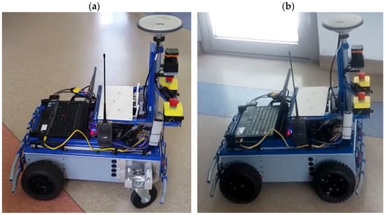
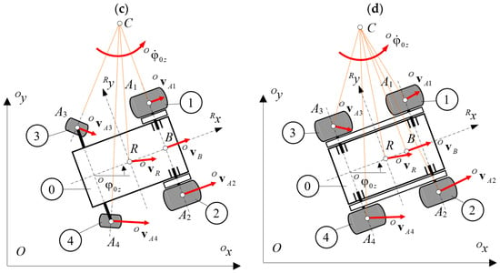
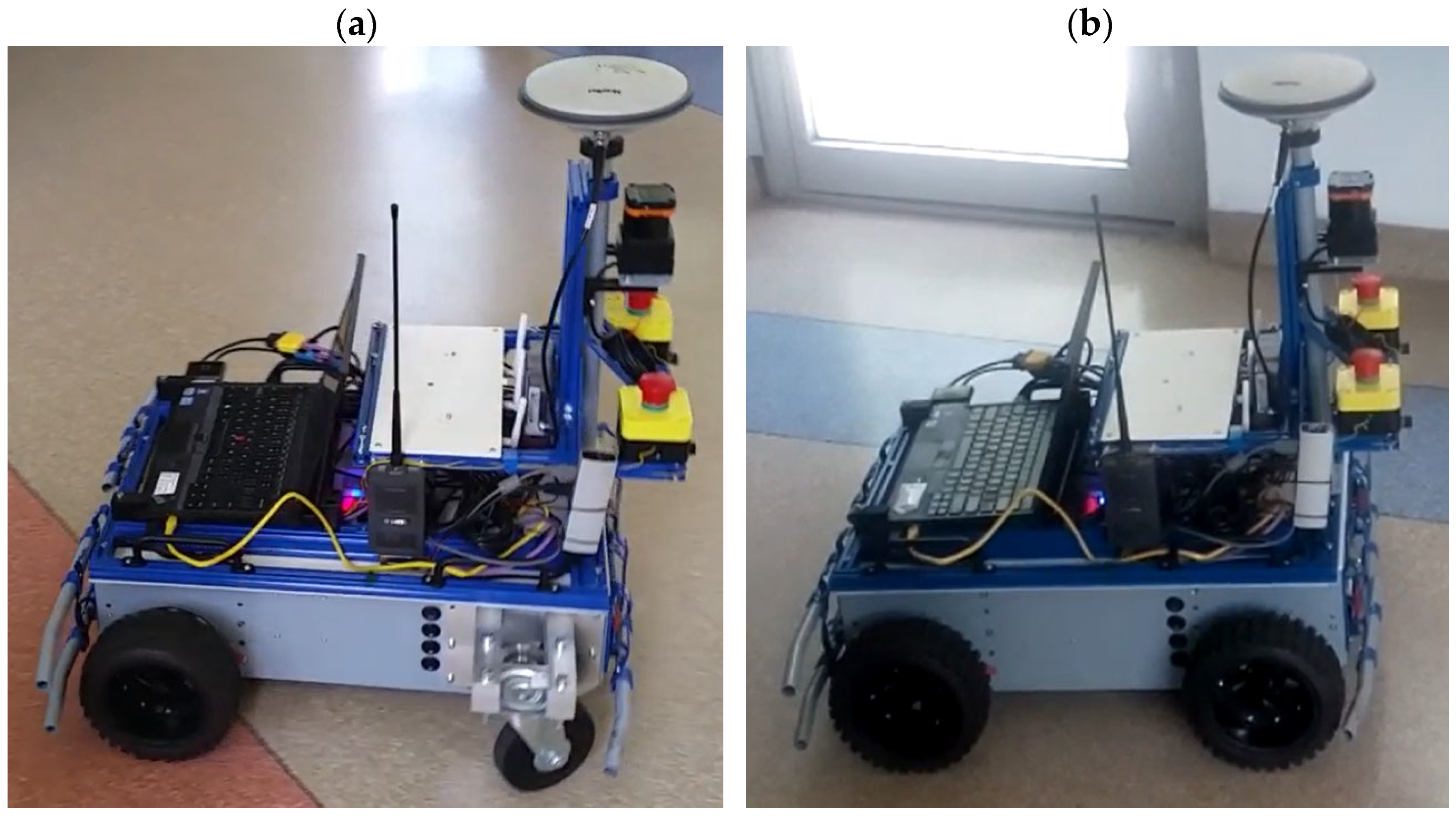
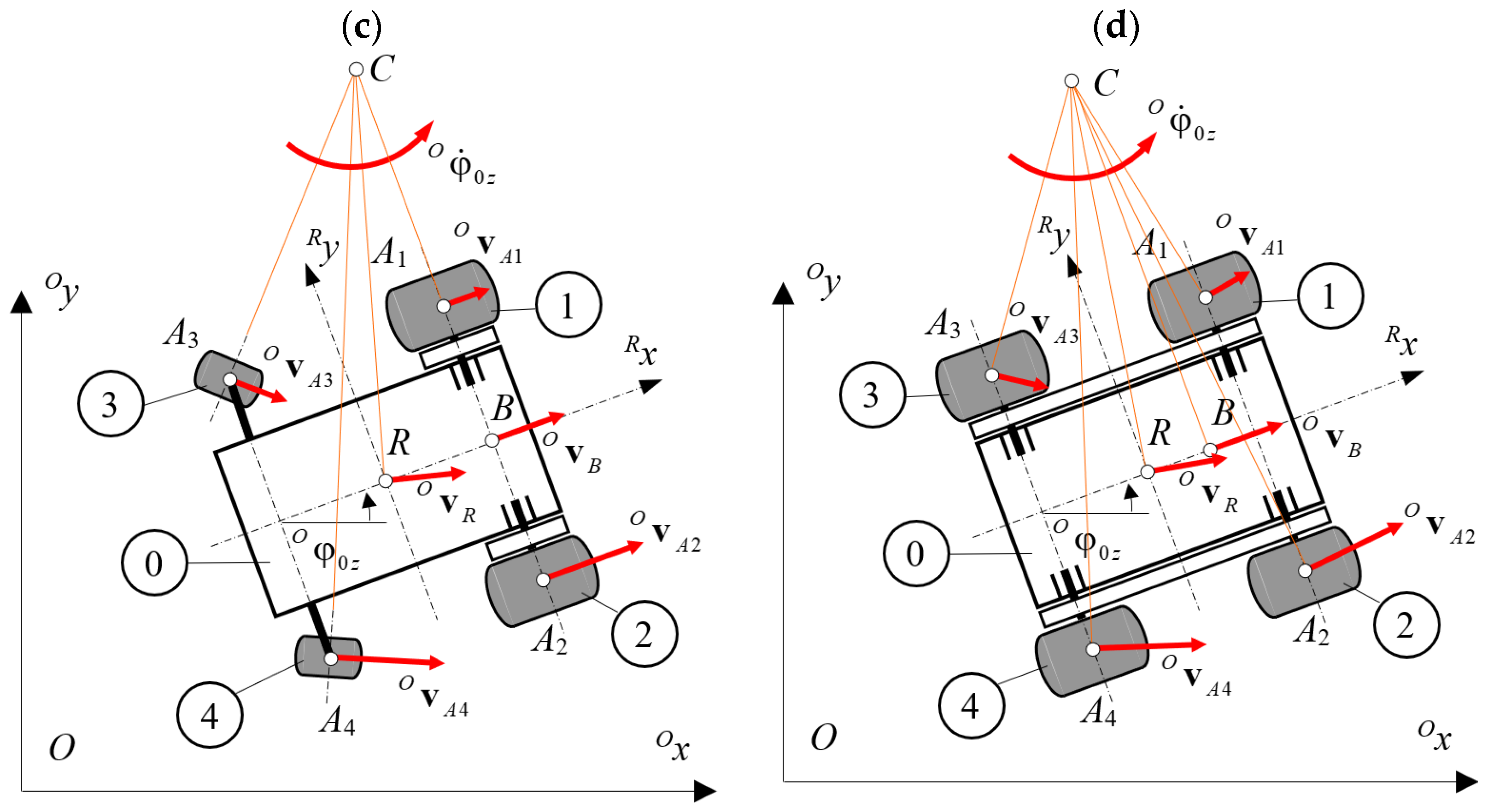
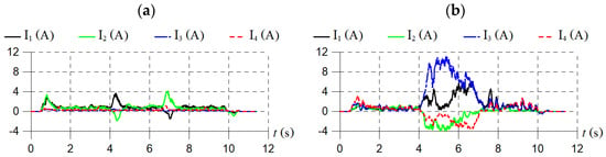
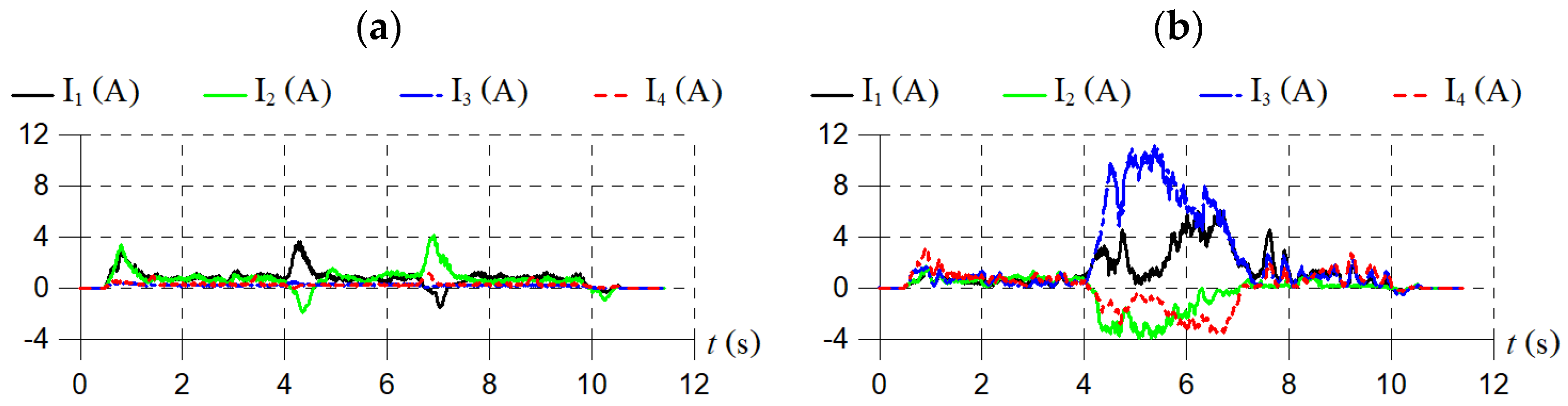
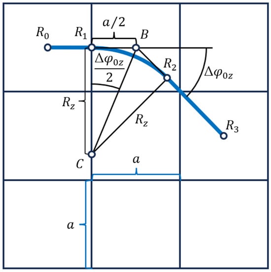
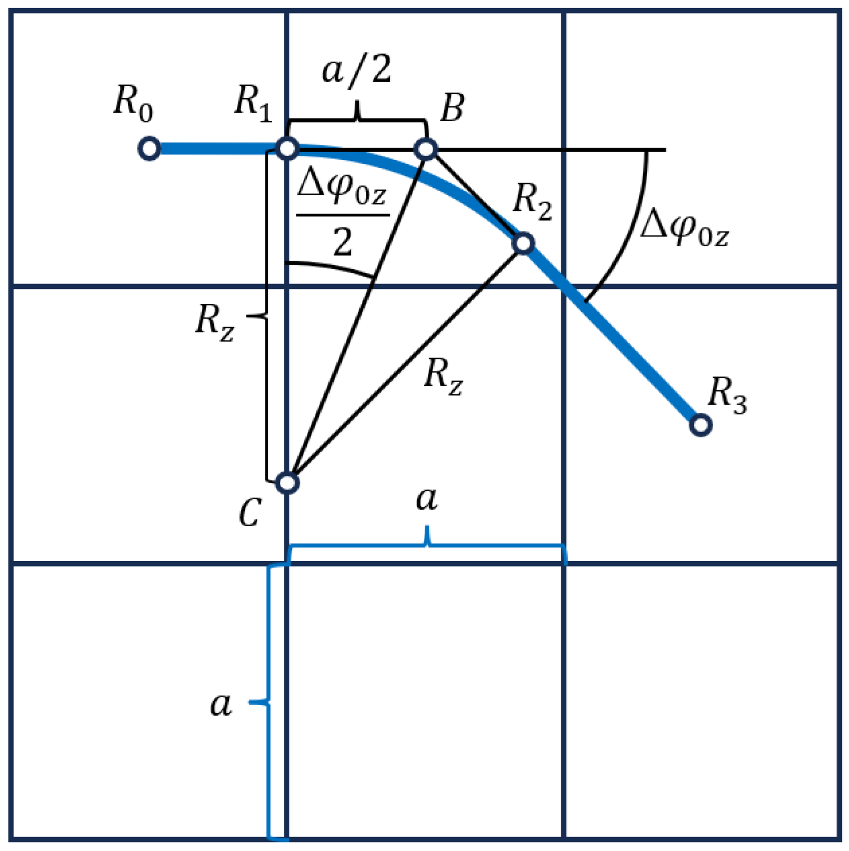
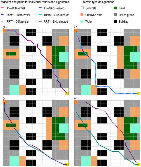
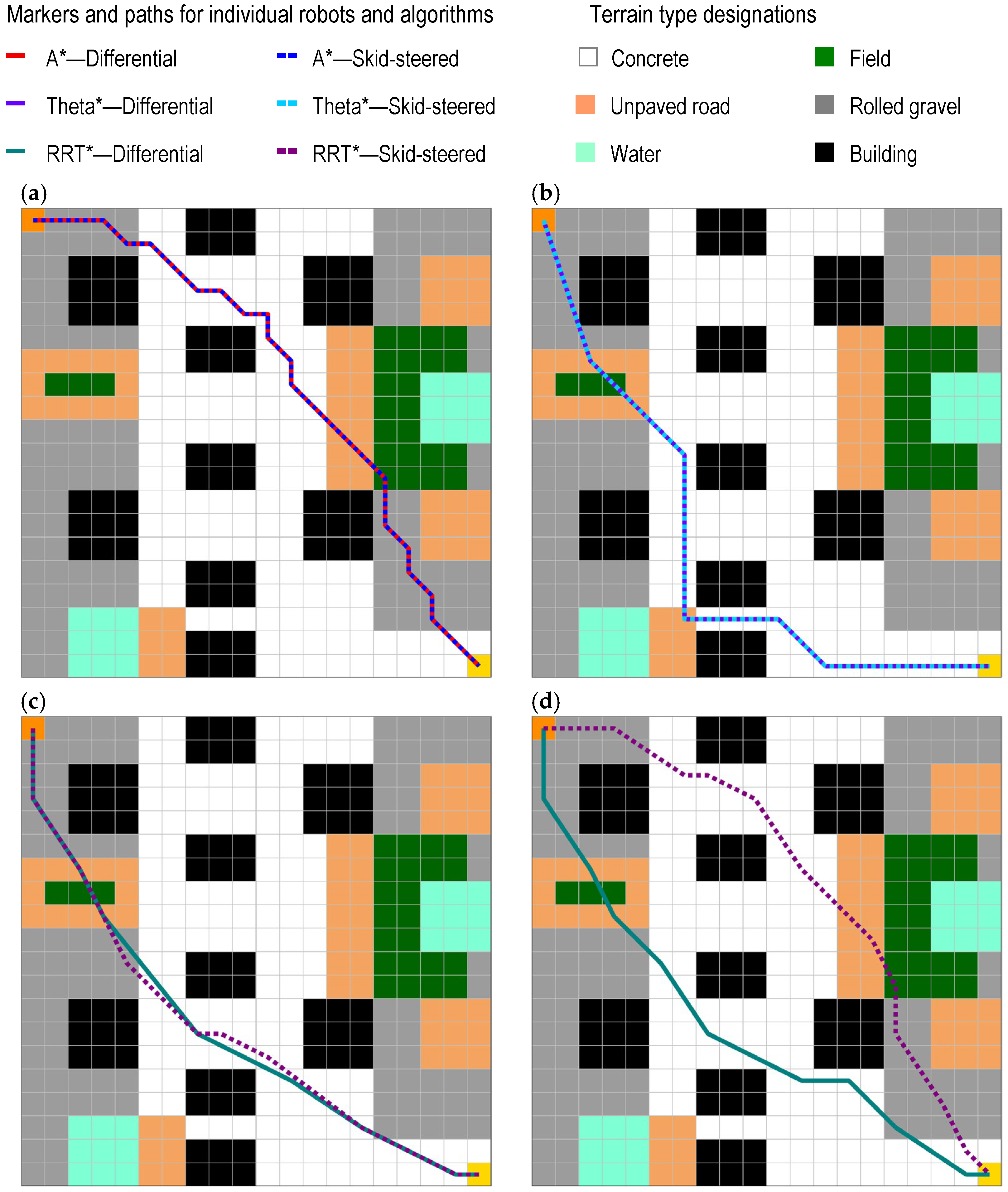
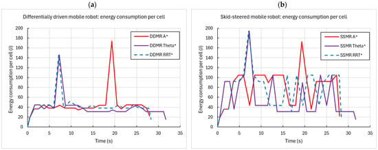
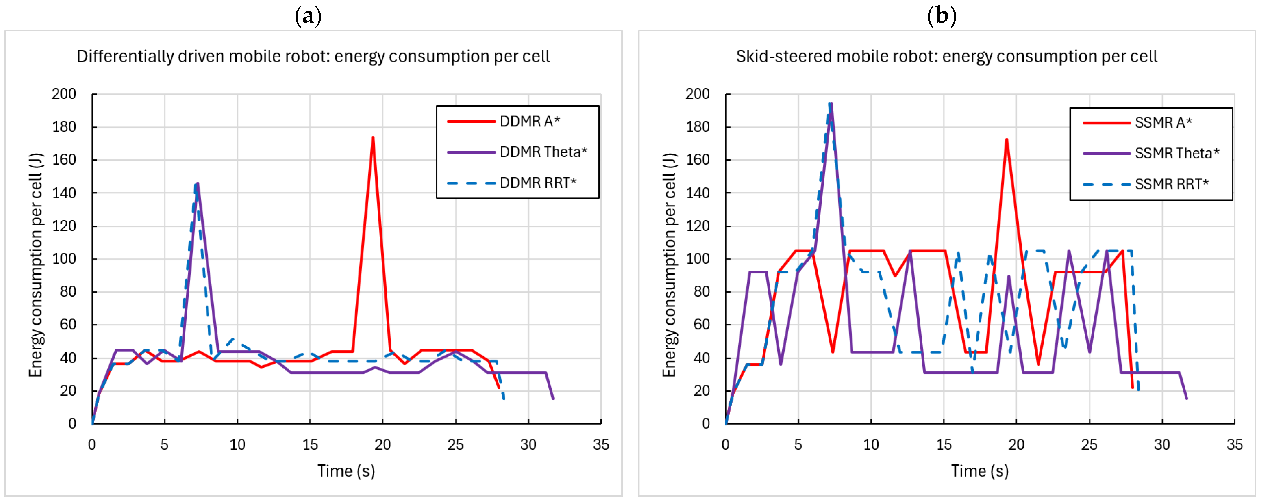
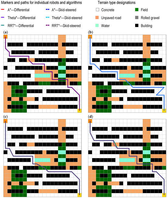
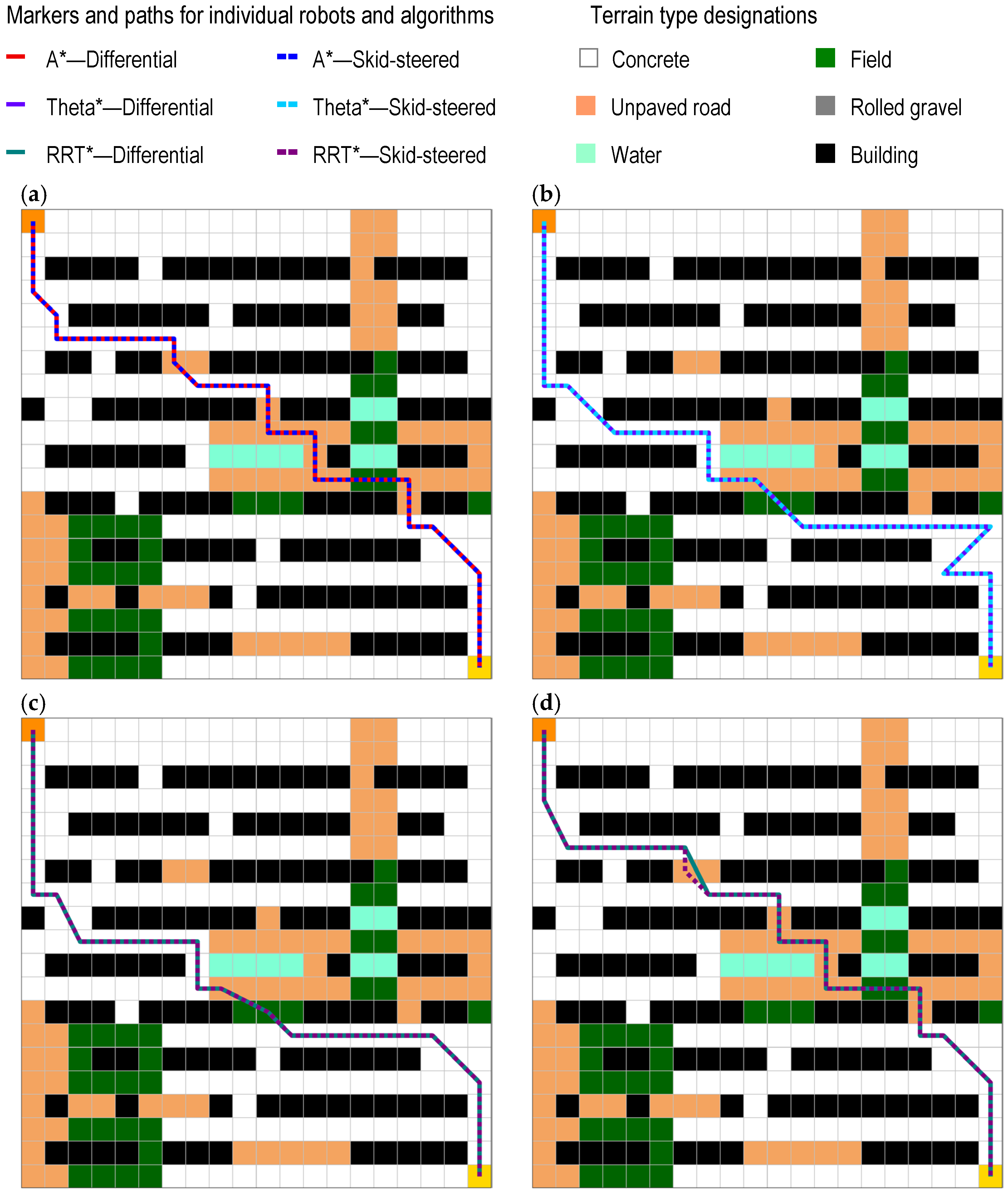
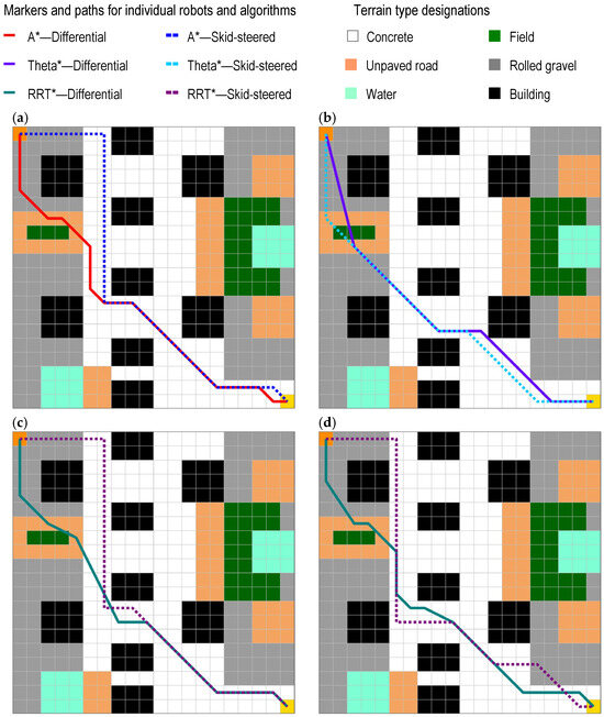
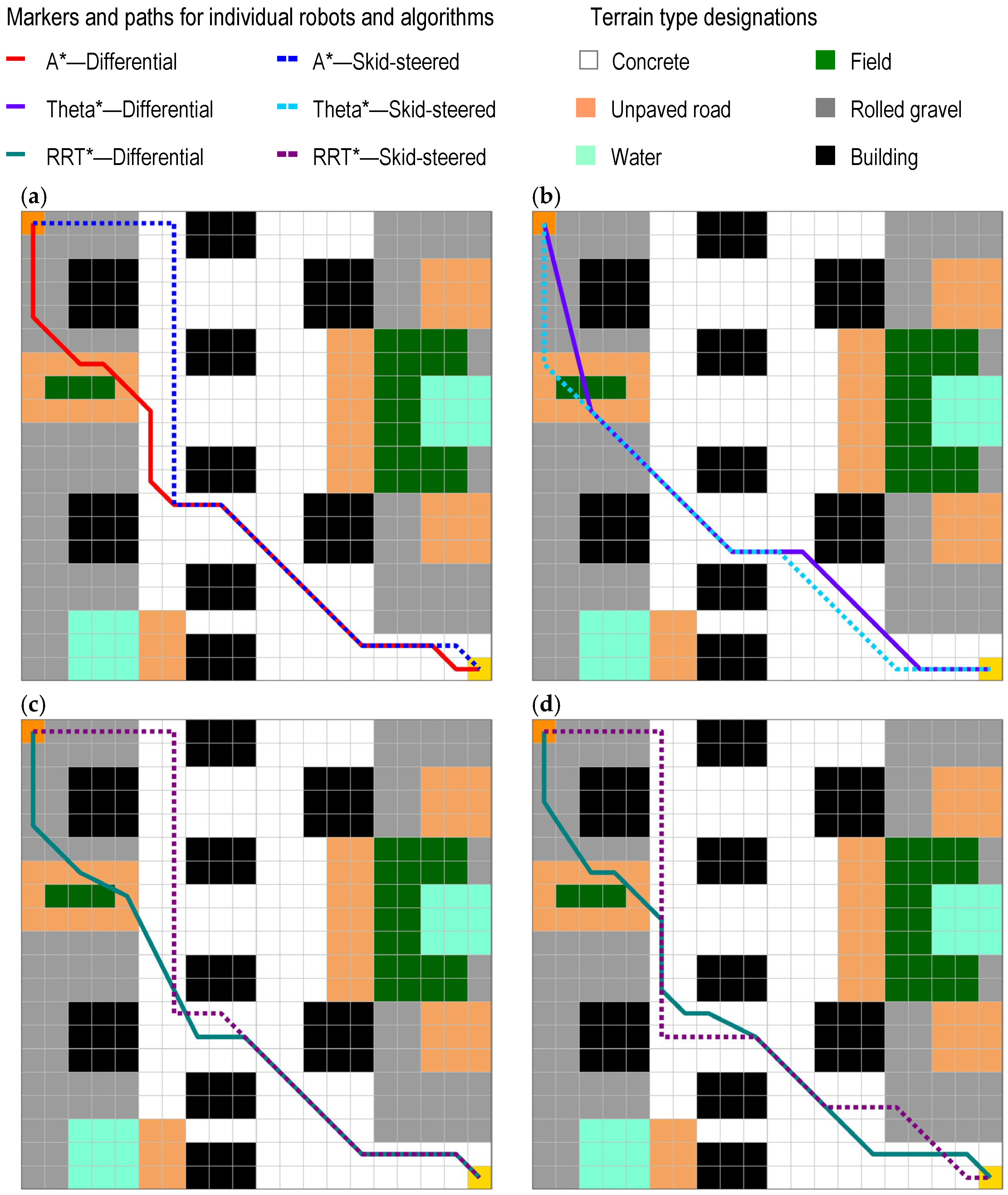
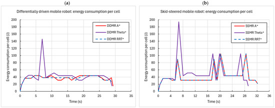
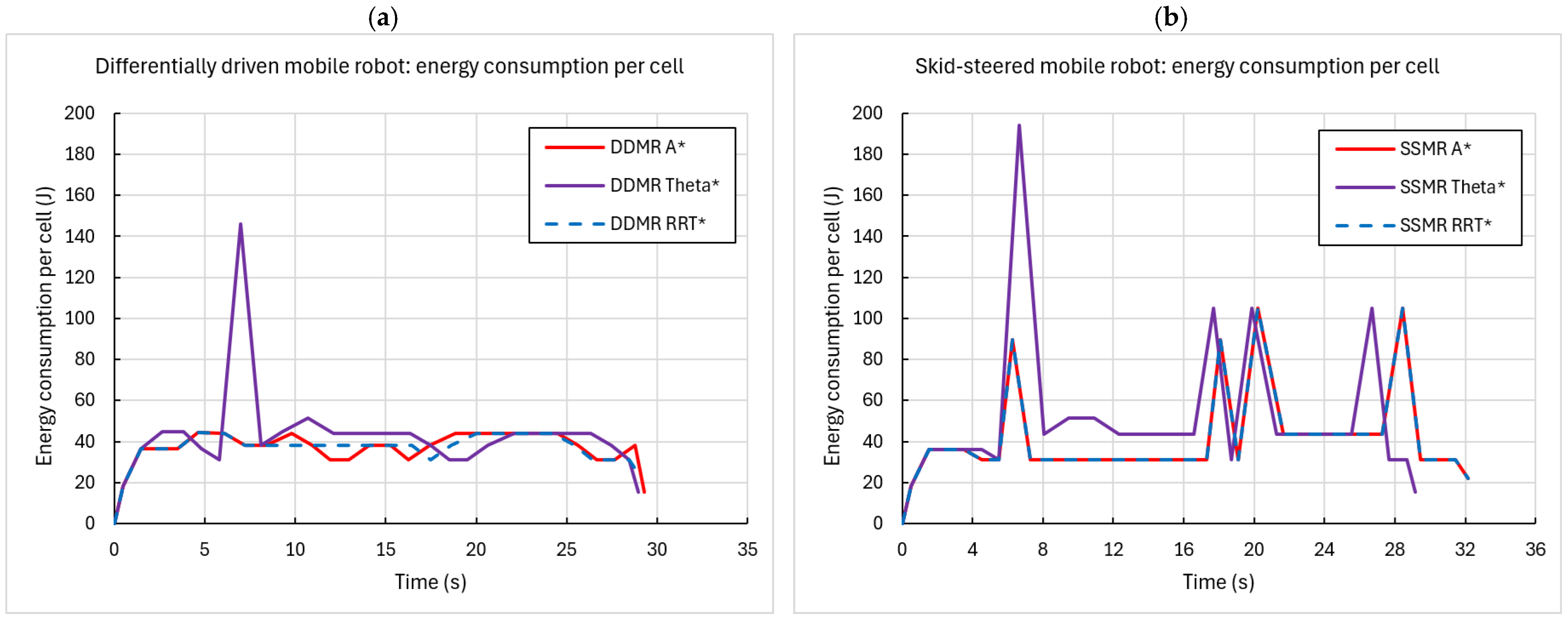
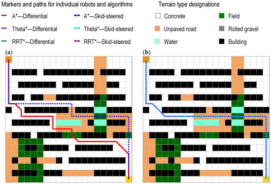
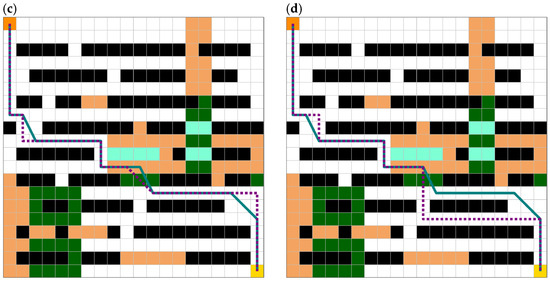
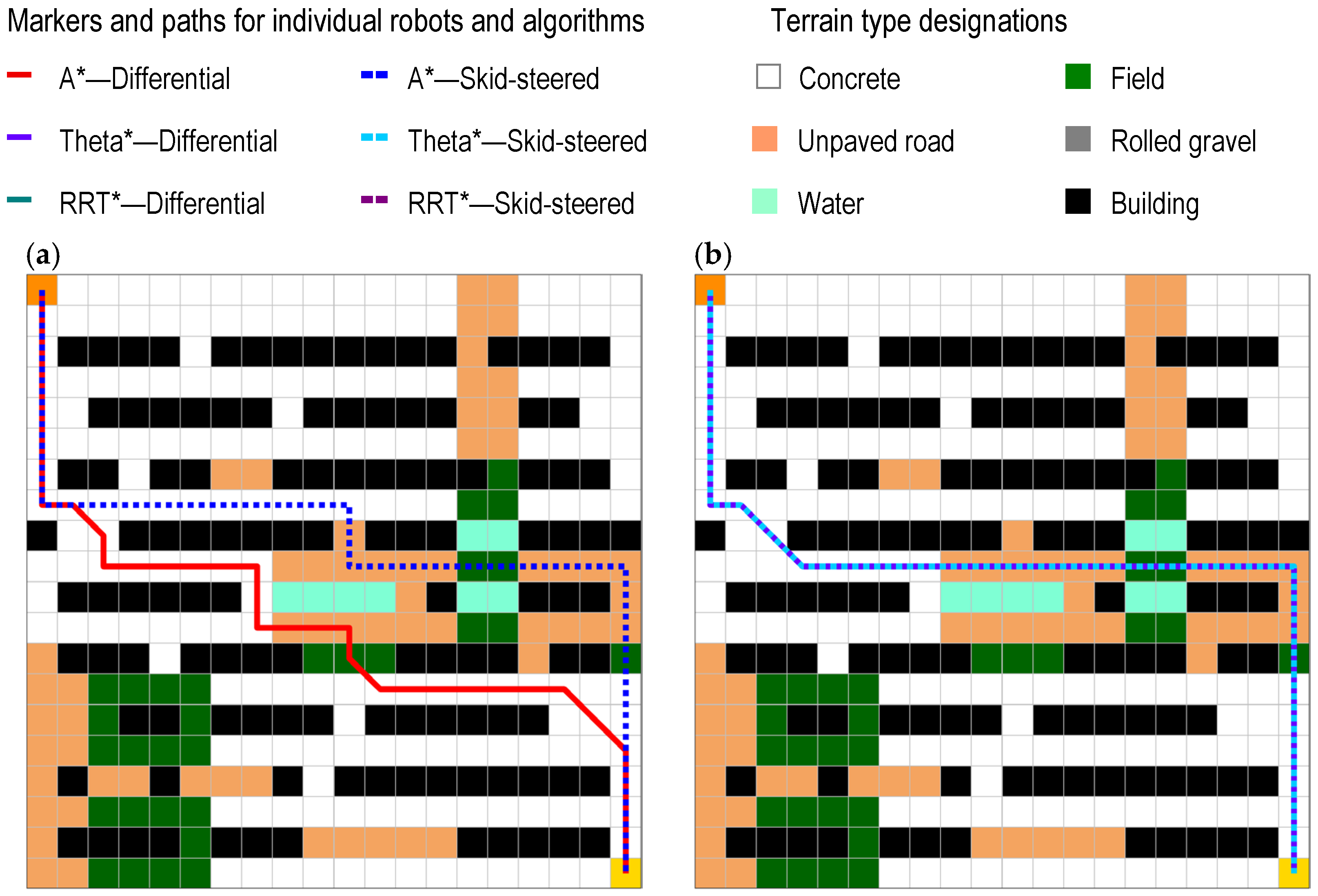
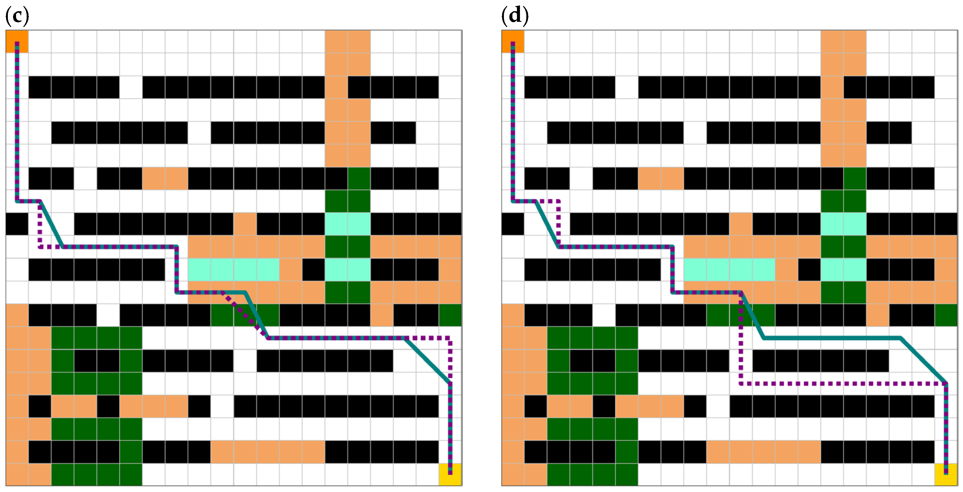
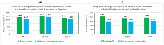
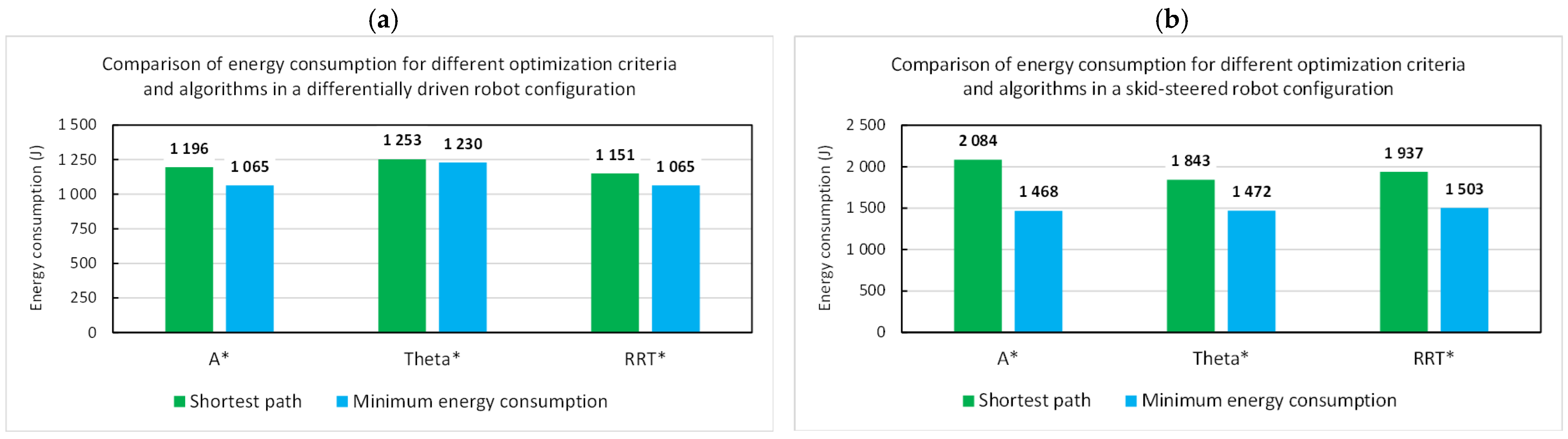
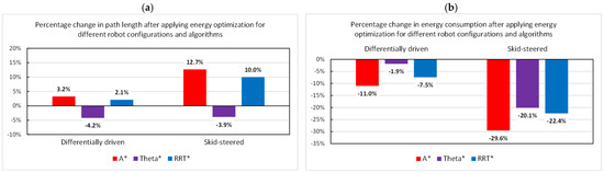
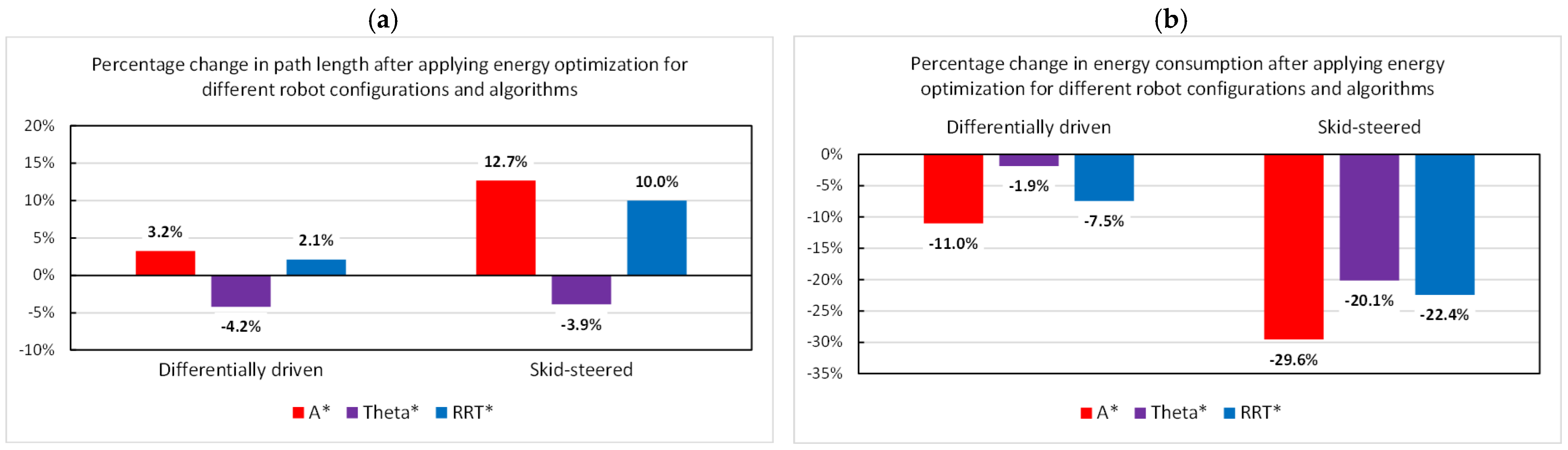

Disclaimer/Publisher’s Note: The statements, opinions and data contained in all publications are solely those of the individual author(s) and contributor(s) and not of MDPI and/or the editor(s). MDPI and/or the editor(s) disclaim responsibility for any injury to people or property resulting from any ideas, methods, instructions or products referred to in the content. |
© 2026 by the authors. Licensee MDPI, Basel, Switzerland. This article is an open access article distributed under the terms and conditions of the Creative Commons Attribution (CC BY) license.