


Abstract
In cyber-physical power systems (CPPS), the inrush current generated during transformer reclosing can easily cause misjudgment of protection devices and thus serves as an important trigger for cascading failure propagation. Existing studies mostly rely on black-box electromagnetic transient simulations or simplified magnetization models, lacking analytical approaches that account for hysteresis and residual magnetism, and therefore fail to accurately characterize the coupling mechanism between physical transients and information-layer dynamics. To address this issue, an analytical transient model for three-phase transformer reclosing is established based on the Jiles–Atherton theory, in which the hysteresis loop and residual magnetism are embedded into the electromagnetic transient process as a differential–algebraic equation (DAE) set, and the semi-analytical dependence of the inrush peak, harmonic characteristics, and decay law on the residual flux and closing angle is derived. On this basis, an inrush-feature-driven probability model of protection misjudgment is constructed, a CPPS cascading failure propagation model incorporating physical–information state transitions is developed, and an adaptive reclosing recovery control strategy based on the node fault-state reachability is proposed. Simulations on the IEEE 39-bus system show that the proposed model accurately reproduces the quantitative influence of hysteresis residual magnetism on inrush characteristics (the peak error is within 10% compared with measured/detailed simulation results), and the proposed control strategy reduces the misjudgment rate per reclosing operation from 6.78% to 1.18% (a reduction of approximately 83%) and the post-recovery load loss from 0.182% to 0.001%, compared with the conventional reclosing scheme, significantly improving the resilience and recovery efficiency of the CPPS.
1. Introduction
1.1. Background and Significance
A cyber-physical power system (CPPS) integrates wide-area measurement, communication networks, and coordinated control deeply into the conventional power grid, enabling real-time perception and optimized regulation of system operating states. However, the deep coupling between the physical grid and the information network also allows local disturbances to spread rapidly through both the “electrical connection” and the “information interaction”: erroneous measurements or failures in the information layer may mislead dispatching decisions, while cascading tripping in the physical layer may in turn destroy the power supply basis of information nodes. Cascading failures have therefore become a major threat to the secure operation of large power grids. Post-event analyses of major blackouts have shown that maloperations or failures to operate of protection and control devices, as well as erroneous information on which dispatching decisions are based, are often the key amplifying links in the evolution of small disturbances into system-wide incidents [1,2,3]. To characterize the cascading mechanism under physical–information coupling, extensive studies have been carried out: a comprehensive review of cyber-physical cascading failures and resilience assessment of power grids is given in [4]; the interdependent propagation of failures between the cyber and physical layers is characterized in [5,6,7] based on interdependent networks and dynamic modeling; and an analytical framework for CPPS cascading failures from the perspective of complex network theory is provided in [8].
Among various disturbance sources, the inrush current produced during transformer reclosing is a long-standing yet insufficiently appreciated risk source. Statistics show that about 80–90% of overhead-line faults are transient, making automatic reclosing one of the most frequently performed operations in power systems [9]. At the reclosing instant, if the closing phase unfavorably superimposes on the residual magnetism of the transformer core, the core becomes deeply saturated and generates an inrush current with an amplitude of 5–8 times the rated current [9]. From the viewpoint of differential protection, the inrush current exhibits a “single-side inflow” characteristic that is highly similar to an internal short-circuit fault; when the second-harmonic content of the inrush is low or the current transformer (CT) is saturated, the harmonic-restraint criterion may fail and cause a false trip [10,11,12]. A single false trip has limited impact by itself, but the resulting power-flow redistribution may induce overloads and cascading tripping of adjacent equipment, becoming the “first domino” of a cascading failure. In the CPPS context, the false status information produced by misjudgment may further mislead dispatching and control decisions through the information layer, forming a vicious circle of “physical disturbance—information misjudgment—physical escalation”. Therefore, establishing an inrush analytical model that accounts for hysteresis residual magnetism and quantitatively links it to the cascading failure propagation mechanism is of great significance for the security defense of CPPS.
1.2. State of the Art
- (1)
- Modeling of transformer reclosing inrush. Mainstream methods fall into three categories: simplified analytical models based on a single-valued or piecewise-linear magnetization characteristic [9], which are computationally efficient but cannot describe residual magnetism and the hysteresis loop and therefore systematically underestimate the inrush peak; black-box models based on electromagnetic transient simulation or finite-element analysis [13], which are accurate but can hardly provide explicit dependence of the inrush on the residual flux and closing angle, and thus cannot be embedded into upper-level propagation models for parametric analysis; and hysteresis models based on the Preisach or Jiles–Atherton (J–A) theory, among which the J–A model has clear physical meaning of its parameters and is easy to embed into circuit equations [14]. Its parameter identification is addressed in [15] using differential evolution, and the J–A model is further extended to low-frequency transients of transformers and shell-type transformer modeling in [16,17]. However, coupling the J–A model with the whole three-phase reclosing transient process and deriving semi-analytical expressions of inrush characteristics remain rarely studied.
- (2)
- Protection misjudgment and cascading failures. In investigations of major North American blackouts, Phadke and Thorp [18] and Tamronglak et al. [19] confirmed that hidden failures of protection systems are an important driving force of cascading events; a cascading dynamics model with protection hidden failures is established in [2]. However, most cascading failure models simplify protection behavior as an ideal “trip on overload” logic or describe maloperation with an exogenous probability, lacking mechanistic modeling at the level of “electromagnetic transient characteristics—protection criterion response”; consequently, the misjudgment probability is decoupled from the operating conditions (residual flux, closing angle).
- (3)
- Cascading failure propagation modeling and recovery control. Complex network theory provides important analytical tools for cascading propagation: Pagani and Aiello [20] comprehensively reviewed the application of complex network theory to power grids; critical nodes are identified based on complex-network centrality in [21]; a cooperative framework for evaluating critical nodes and enhancing robustness is proposed in [22]; and the performance and reliability evolution of power grids under cascading failures is studied in [23]. For recovery control, critical load restoration using distributed energy resources, resilience-oriented microgrid restoration, and a review of restoration techniques are presented in [24,25,26], respectively. These works generally simplify the physical grid as a power-flow graph and the information layer as an independent failure process, and rarely consider how the physical transient of reclosing inrush is transformed into a cascading trigger source through protection misjudgment; a coordinated control design of ‘physical-source suppression (controlled switching) + information-side blocking (recovery priority)’ targeting this mechanism is also lacking. As for controlled switching, [27,28,29,30] demonstrated that inrush can be significantly suppressed or even eliminated by residual-flux prediction and phase control; however, existing studies target a single machine or substation protection and have not evaluated the system-wide value of controlled switching in the overall framework of CPPS cascading defense.
1.3. Research Gaps
The main deficiencies of existing studies are as follows:
- (1)
- at the inrush modeling level, an analytical model that accounts for hysteresis residual magnetism and provides explicit dependence of inrush characteristics is lacking, so that physical transients cannot be “translated” into upper-level CPPS propagation analysis;
- (2)
- at the coupling-mechanism level, a quantitative mapping of “inrush characteristics → misjudgment probability → cascading trigger” is absent, and the misjudgment events are decoupled from operating conditions, which distorts the trigger mechanism of cascading models;
- (3)
- at the control-design level, conventional reclosing control (e.g., fixed time-delay reclosing) is unaware of residual flux and node criticality, and recovery strategies do not distinguish the “leverage” differences in nodes in cascading propagation, making coordinated dual-side blocking difficult.
1.4. Contributions
To address the above problems, the main contributions of this paper are as follows:
- (1)
- An analytical transient model of three-phase transformer reclosing based on the J–A theory is established: the hysteresis differential equation is coupled with the three-phase transformer electromagnetic equations as a differential–algebraic equation (DAE) set, the residual magnetism is naturally embedded into the closing process as the initial value, and semi-analytical expressions of the inrush peak, harmonic characteristics, and decay time constant with respect to the residual flux and closing angle are derived based on flux conservation. Unlike existing single-technique studies, the three components form a closed analytical chain in which the electromagnetic transient (the J–A model), the protection response (the misjudgment probability model), and the system behavior (the cascading propagation model) are mutually consistent: the same residual-flux–closing-angle quantities drive all three levels, which allows the cascading trigger source to be traced back to a physical mechanism rather than an exogenous assumption.
- (2)
- An inrush-feature-driven probability model of protection misjudgment is constructed, a CPPS cascading failure propagation model incorporating physical–information state transitions is developed, and the node fault-state reachability index is proposed to quantify the criticality of nodes in cascading propagation.
- (3)
- An adaptive reclosing recovery control strategy based on reachability is proposed: on the physical side, inrush is suppressed at the source through residual-flux prediction and optimal closing-angle selection; on the information side, propagation chains are blocked by prioritizing the recovery of high-leverage nodes. IEEE 39-bus system simulations show that, compared with the conventional reclosing scheme, the misjudgment rate per reclosing operation and the post-recovery load loss are reduced by approximately 83% and 99%, respectively.
1.5. Organization
Section 2 presents the overall CPPS architecture and problem formulation, and then establishes the J–A reclosing transient model, the misjudgment probability model, the cascading propagation model, and the recovery control strategy, followed by the case-study settings. Section 3 reports the simulation results and analysis. Section 4 discusses the mechanistic implications, the differences from existing studies, and the engineering applicability. Section 5 concludes the paper. Appendix A gives the parameter identification of the J–A model and the derivation of the inrush peak approximation.
2. Materials and Methods
2.1. Overall CPPS Architecture and Problem Formulation
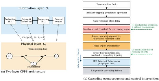
The CPPS considered in this paper consists of a physical power grid and an information network coupled in two layers. The physical layer is represented by a weighted graph , whose nodes are generators and substation buses and whose edges are transmission lines and transformer branches with power flows as weights. The information layer is represented by a graph , whose nodes are protection devices, measurement and control units, and the control center, and whose edges are communication links. The two layers are coupled through the mapping : each physical node is protected, measured, and controlled by its corresponding information node; the failure of an information node renders its mapped physical node “out of control”, manifested as protection miscoordination, unobservable states, or unreachable control commands.
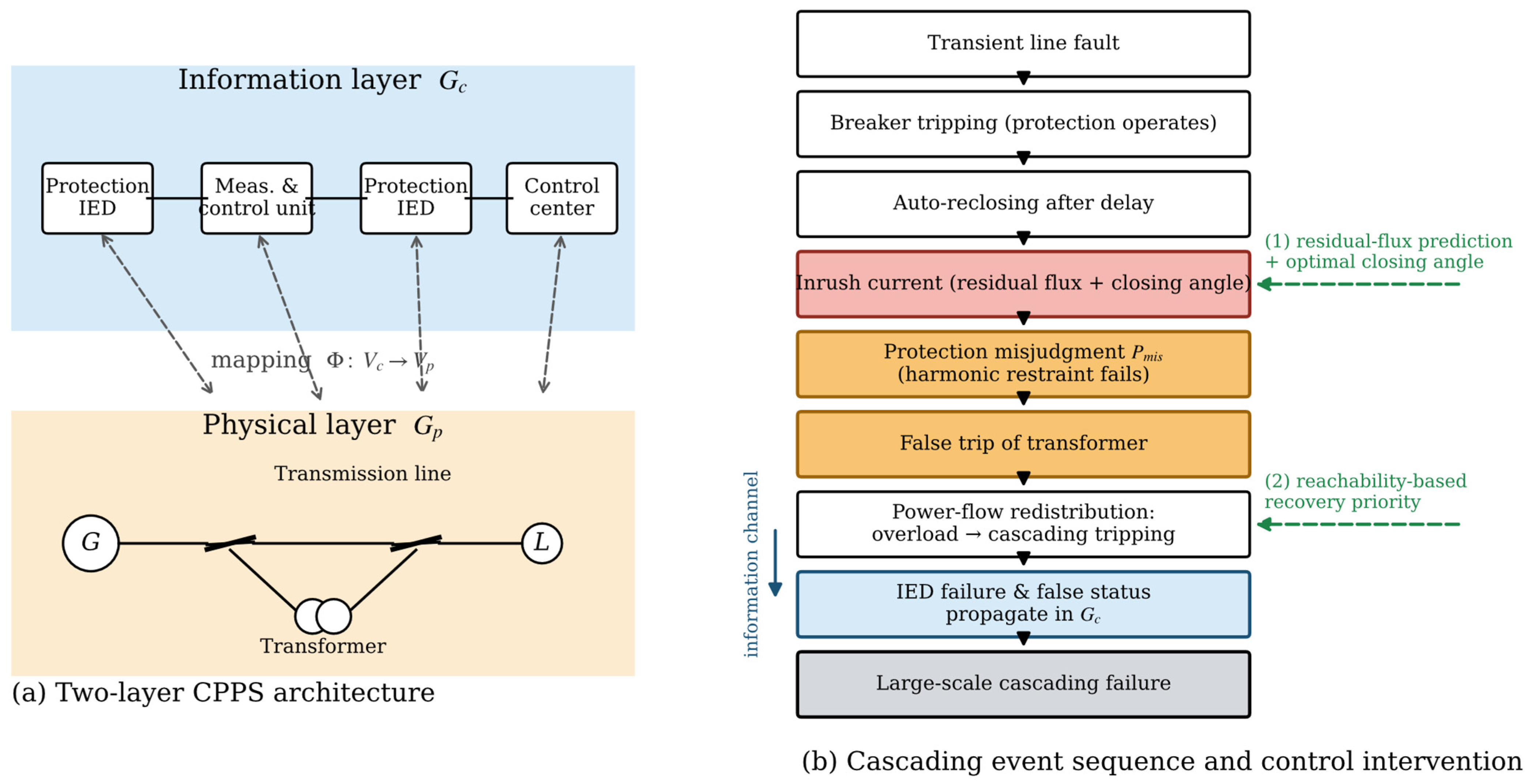
The cascading event sequence of concern in this paper is as follows: a transient fault occurs on a line → protection operates and the breaker trips → automatic reclosing after a time delay → the reclosing inrush acts on the transformer differential protection → misjudgment occurs with a certain probability and falsely trips the transformer → power-flow redistribution induces overload and cascading tripping of adjacent equipment → failures and false states propagate synchronously in the information layer → if not blocked in time, a large-scale cascading failure evolves. In this sequence, the inrush is the physical trigger source, the misjudgment is the physical–information coupling interface, and the power-flow transfer and information failure are the propagation channels; recovery control needs to intervene cooperatively on two time scales, “before the inrush is produced” and “while the propagation is forming”. The overall architecture and the event sequence are shown in Figure 1.
Figure 1.
Two-layer CPPS architecture and the cascading event sequence triggered by the reclosing inrush.
On the IEEE 39-bus system, the event sequence is implemented as follows. A line is selected at random as the faulted element; the breakers at both ends of the line open, the line is removed from the network, while the step-up transformers at the terminal buses remain connected to the grid through their low-voltage windings. After a reclosing delay of 0.5 s, the line is re-energized. The reclosing inrush flows into the local step-up transformer, whose differential protection is then subject to misjudgment sampling according to Equation (8); if misjudgment occurs, the transformer branch is tripped and locked out. During the recovery stage, each restored transformer branch is re-energized through a new reclosing operation with the same misjudgment sampling. The initial magnetization state of every reclosing event is set as M(0) = Φx/μ0, where Φx is the residual flux estimated from the voltage integral before the preceding trip (Appendix A.2); for uncontrolled reclosings, the closing angle is drawn from U(0°, 360°), whereas controlled reclosings use θ* = 90°/270°.
2.2. J–A-Theory-Based Transient Model of Three-Phase Transformer Reclosing
2.2.1. Hysteresis Model
The J–A theory decomposes the magnetization M into the anhysteretic magnetization and an irreversible component. The anhysteretic magnetization is described by the Langevin function:
where is the saturation magnetization; a is the shape parameter of the anhysteretic magnetization; is the domain-wall coupling coefficient; and is the effective field intensity. The differential susceptibility of the total magnetization is
where is the pinning loss coefficient; is the reversible magnetization coefficient; and is the direction parameter, taking +1 when and −1 otherwise. Equations (1) and (2) completely characterize the hysteresis loop; the residual magnetism , i.e., the intersection of the loop with the M-axis, is uniquely determined by the model parameters, which makes “how much flux remains in the core after tripping” a computable quantity rather than an exogenous setting. The parameters and can be identified from the no-load test data of the transformer (see Appendix A). The classical Langevin expression has limited fitting accuracy in the transition region between the linear and saturated segments of the magnetization curve. To improve the fitting accuracy in the transition region, a modified Langevin expression can be used to describe the anhysteretic magnetization: when ,
and it degenerates to the classical expression when . The modified model can simulate various hysteresis loops more accurately while keeping the domain-theory framework unchanged.
2.2.2. DAE Model of the Three-Phase Transformer Electromagnetic Transient
For a three-phase two-winding transformer, let . The voltage equation and magnetic circuit constraints of each phase are
In Equation (3), the term Lσdi1j/dt accounts for the leakage inductance of the winding: together with the magnetizing-branch inductance of the J–A model it forms the total series inductance of the circuit, so that the leakage inductance enters the DAE set both through Equation (3) and through the parameter vector p, where and are the resistance and number of turns of the primary winding; and are the core cross-sectional area and equivalent magnetic path length; is the magnetizing current; and is the secondary current referred to the primary side. The constitutive relation of the magnetizing branch is given by the J–A model, i.e., Equations (1) and (2). Combining Equations (3)–(5) with the J–A equations yields a differential–algebraic equation set with the magnetization and winding currents of each phase as state variables, where the parameter vector is and is the leakage inductance.
In matrix form, the three-phase coupled model is written as above, where Cw is the 3 × 3 identity matrix (Cw = I3 × 3) for the Yd11 connection studied in this paper, and i′2 = [i′2a, i′2b, i′2c]T collects the delta-winding currents referred to the primary side; the delta connection is then imposed through the algebraic constraint i′2a + i′2b + i′2c = 0, and the primary-side neutral-point voltage uN enters the voltage balance as an additional unknown determined by the floating-neutral condition. For the other connections mentioned in Section 2.2.5 (Ynd11, Yny0, Yy0), Cw takes the corresponding form together with the associated neutral or delta constraint; the three-phase equation set is integrated simultaneously with the J–A constitutive Equations (1) and (2) by the procedure described above.
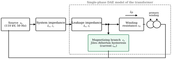
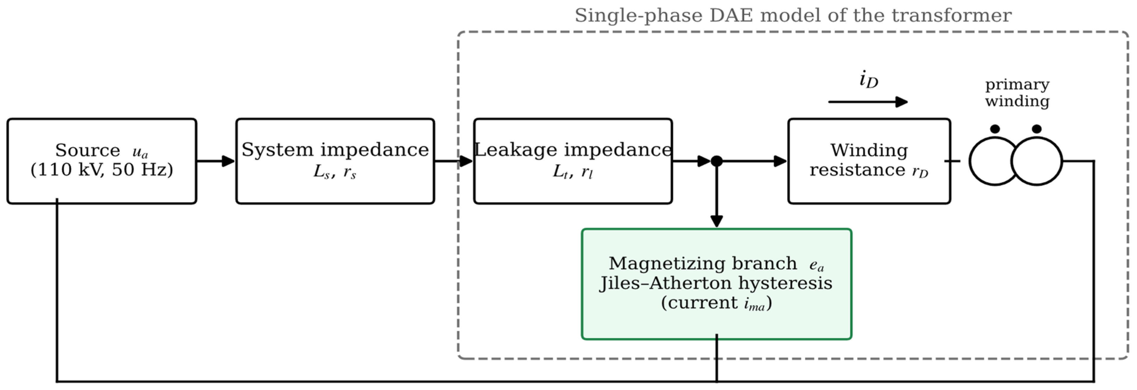
The DAE set is solved by a field–circuit coupled method: taking the field intensity and the flux density of each phase as state variables, the voltage balance Equation (3) is combined with the J–A constitutive equations and discretized by the backward Euler method into a set of nonlinear algebraic equations, which is then solved iteratively by the Newton–Raphson method; the Jacobian matrix at each time step is composed of the partial derivatives of the J–A rate equation with respect to the state variables. This solution procedure applies to both the classical and the modified J–A models, and has been verified against measured short-circuit test currents in our previous work on transformer short-circuit modeling (errors of 5–22%, with the largest error at the deepest saturation; see Section 3.1). The overall structure of the model is shown in Figure 2.
Figure 2.
Block diagram of the single-phase DAE model of the transformer.
2.2.3. Initial Residual Flux and the Reclosing Process
After the line trips, the transformer is disconnected from the grid, the winding voltage becomes zero, and the core flux decays along the J–A loop and stabilizes at the residual flux (the flux corresponding to ). Let be the reclosing instant and the closing angle (referred to the zero crossing of the phase voltage), with the phase voltage . From flux conservation, the core flux after closing is approximately
where is the amplitude of the steady-state flux and is the decay time constant of the flux after tripping, which describes the relaxation of the flux toward the remanence point through core (hysteresis and eddy-current) losses; τΦ is identified here from the decay of the no-load flux after switch-off. Equation (6) shows that the flux at the closing instant consists of an alternating component superimposed on a bias component having the same sign as the residual flux (including the ). When and superimpose in the same direction and push beyond the saturation flux , the core saturates and inrush is produced. This provides an explicit mechanism for “the larger the residual flux and the more unfavorable the closing angle, the larger the inrush”.
The approximate solution can also be derived directly from flux conservation: after closing, the flux of phase is the superposition of a steady-state periodic component and a transient bias component, i.e., , where the bias flux is determined by the flux conservation condition . It follows that:
- (i)
- when approaches 0° or 180° (closing at voltage zero crossing) and the residual flux has the same polarity as the bias, is maximized, the total flux crosses the saturation flux first, and the inrush is most severe;
- (ii)
- when approaches 90° or 270° (closing at the voltage peak), only the residual-flux component remains in the bias. This conclusion is consistent with Equation (7) and provides a flux-conservation-level theoretical basis for the optimal closing angle later on, namely “avoid the voltage zero crossing and stay close to the voltage peak”.
2.2.4. Semi-Analytical Characterization of the Inrush Characteristics
After core saturation, the magnetizing branch is equivalent to an approximately linear small inductance , so that the semi-analytical approximation of the inrush peak of phase is
where the saturation inductance L0 = Lσ + N12μ0A/le (0.262 H for the test transformer) is the sum of the leakage inductance and the air-core inductance of the saturated branch; Equation (7) is therefore dimensionally consistent, since the flux linkage N1ΔΦ divided by the inductance L0 gives the current. The saturation flux Φs (1.75 T) and a proportionality factor (1.05) are identified by least-squares fitting against the DAE numerical peaks, giving a mean relative error of about 11%, with larger errors near critically saturated conditions (the complete waveform is always provided by the DAE solution). Accordingly, the second-harmonic content of the inrush decreases as the residual flux increases and the closing angle deteriorates (the more severe the waveform distortion and the DC bias), and the decay time constant is approximately (decay of the DC component). It should be noted that Equation (7) is a semi-analytical approximation based on flux conservation, used for analysis of parameter dependence and control design; the complete inrush waveform is obtained by numerically solving the DAE set in Section 2.2.2, and their consistency is verified in Section 3.1.
2.2.5. Three-Phase Coupled Model Considering the Winding Connection
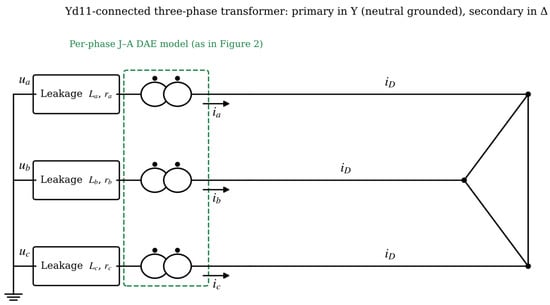
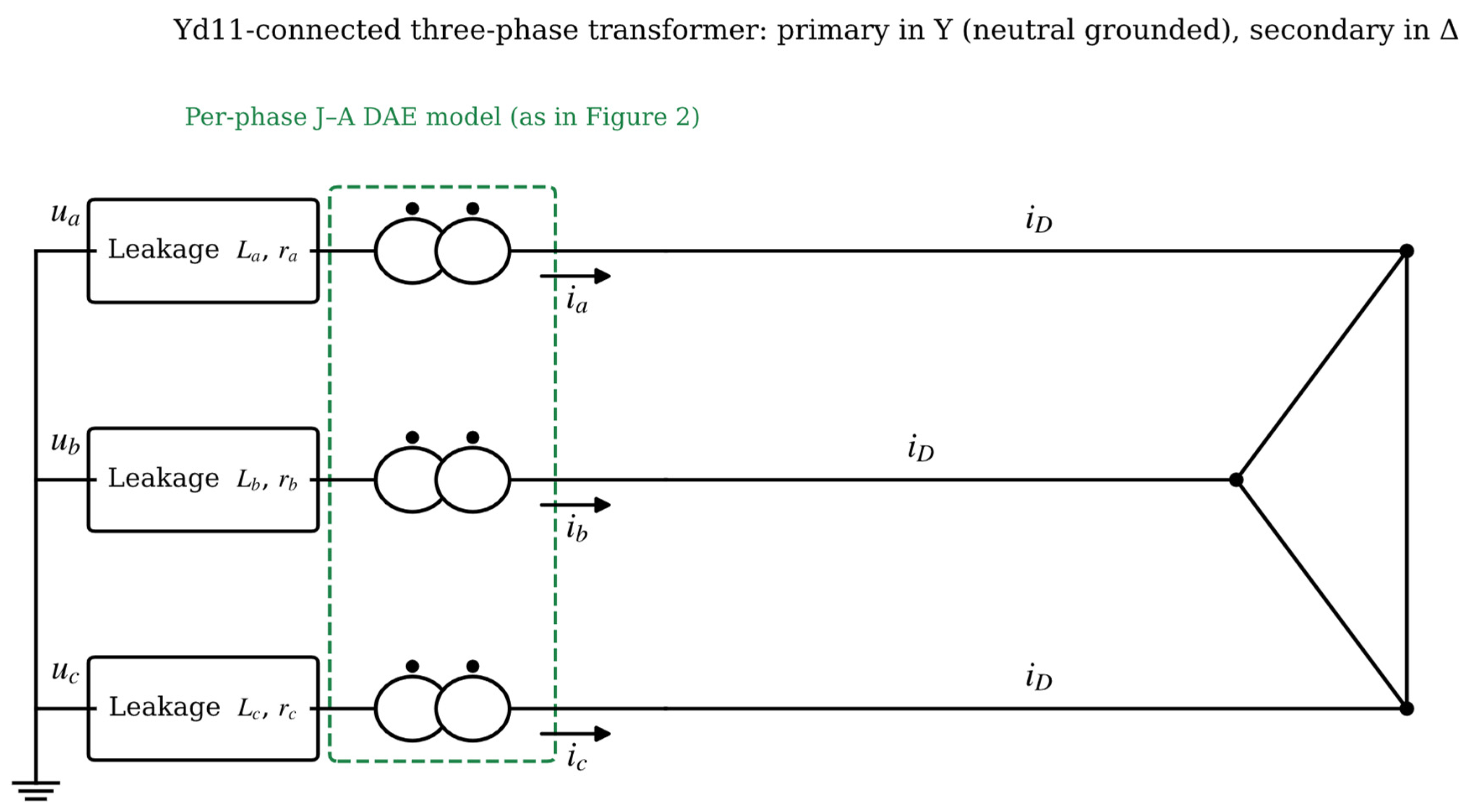
The winding connection of an actual three-phase transformer (Yd11, Ynd11, Yny0, Yy0, etc.) determines the zero-sequence path and the magnetic coupling among phases, and hence the distribution of the bias flux and inrush among phases. Based on the single-phase DAE, the three-phase voltage balance equations are written according to the connection and transformed into matrix form, with the three-phase fluxes as state variables solved uniformly; the overall structure is shown in Figure 3 Taking Yd11 as an example, the neutral-point voltage of the primary Y connection is taken as an additional unknown, and a 3 × 3 differential equation set is obtained after eliminating the primary and secondary current constraints; the treatments of Ynd11, Yny0, and Yy0 are similar, differing in whether the neutral point is grounded and in the current constraints corresponding to the delta or star connection of the secondary side.
Figure 3.
Schematic of the Yd11-connected three-phase transformer (primary in Y with grounded neutral, secondary in delta).
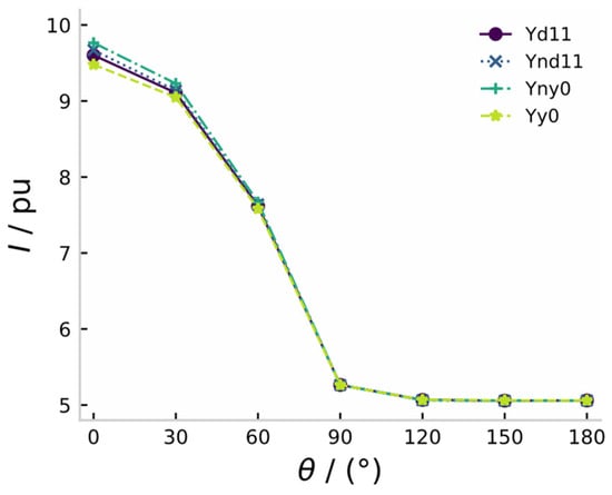
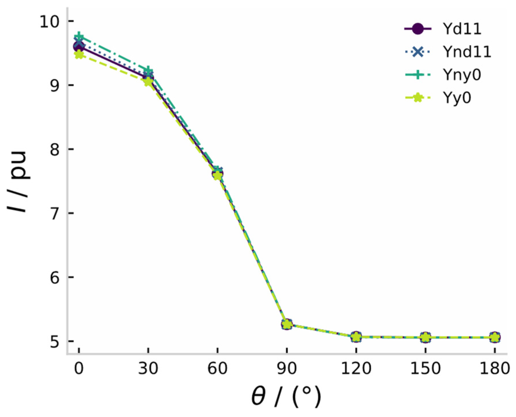
Our previous studies show that when the residual flux of each phase is zero, the winding connection has essentially no influence on the first peak of the phase current, which is determined by whether the closing angle of each phase approaches the voltage zero crossing; when the residual flux is non-zero (e.g.,), the influence of the connection appears: the current peak of the Yny0 connection is the largest and that of the Yy0 connection is the smallest (Figure 4). The transformers modeled in the case study adopt the Yd11 connection, and the above matrix-based method is used to handle the three-phase coupling. The near-overlap of the four curves in Figure 4 is itself a result: the connection-dependent differences are second-order, appearing only at small closing angles (θ < 60°) with a maximum spread of about 3%, so the winding connection is not a first-order factor for the inrush peak.
Figure 4.
Phase-A peak current versus switching angle for four winding connections with non-zero residual flux () (prior analytical results).
2.3. Inrush-Feature-Driven Probability Model of Protection Misjudgment
Whether a differential protection misjudges depends on the relation between the inrush characteristics and the criterion thresholds. Two inrush features are used as the inputs of the model: the peak multiple ( is the rated current), and the second-harmonic ratio ; the decay time constant was examined during feature selection but was found to carry no significant additional information once kI and r2 are given, and is therefore not included in the final model. The effect of CT saturation is not an explicit input either; instead, random CT saturation is applied during the calibration simulations so that its influence is absorbed into the constant term. The final model used in all simulations is:
The coefficients were calibrated on a 9 × 8 grid of residual flux and closing angle with 40 Monte Carlo replications per point, each replicating the ratio-differential criterion with second-harmonic restraint under 2% measurement noise and random CT saturation; logistic regression on the resulting binary outcomes gives β0 = −2.488, β1 = 1.456, β2 = 0.300, with a classification accuracy of 98.6% on the calibration grid. This model quantitatively “translates” physical transient characteristics into information-layer failure probabilities and serves as the interface between Section 2.2 and Section 2.4.
2.4. CPPS Cascading Failure Propagation Model with Physical–Information State Transitions
2.4.1. Node State Machine and Transition Rules
To characterize the physical–information coupled propagation, the operating state of physical node is defined as normal, 1 overload, 2 tripped, 3 out of control, 4 recovered}. The state of an information node is jointly determined by the state of its mapped physical node and the availability of communication links. The state transition rules are as follows:
- (T1)
- Overload transition: if the power-flow calculation gives and the condition persists beyond the allowable overload duration , then : 0 → 2 (cascading tripping);
- (T2)
- Misjudgment trigger: when a reclosing event occurs, the involved transformer node is sampled with probability ; if hit, (false trip), and it is recorded as an “information-induced tripping”;
- (T3)
- Out-of-control transition: if an information node fails (link interruption or node failure) and its mapped physical node loses protection/control reachability, then : ; an out-of-control node cannot be orderly tripped after overload, and its probability and delay of transition to tripping increase significantly;
- (T4)
- Information-failure propagation: the tripping of a physical node may cause the failure of the nodes powering or communicating with it, false state information spreads along , and the dispatcher may issue erroneous control commands to healthy nodes (sampled with probability );
- (T5)
- Recovery transition: after maintenance is completed and the reclosing operation is performed, : , and returns to 0 after checking; the recovery operation itself introduces a new inrush risk and must be suppressed by the strategy in Section 2.5.
2.4.2. Propagation Algorithm and Node Fault-State Reachability
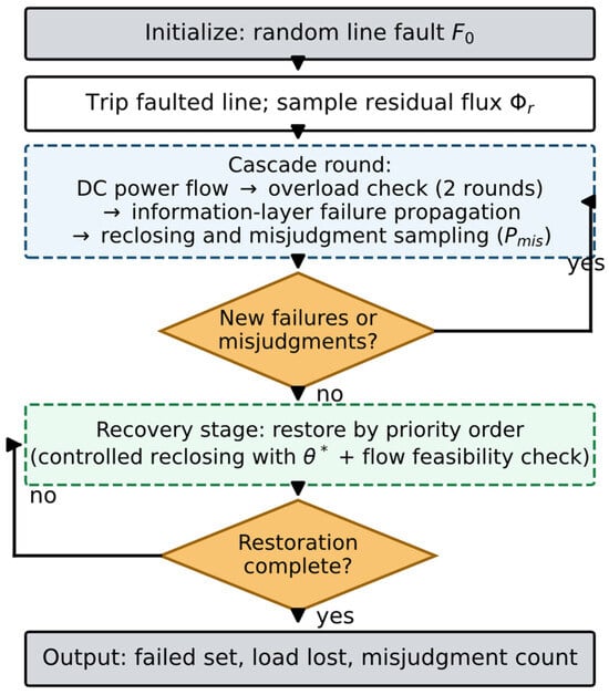
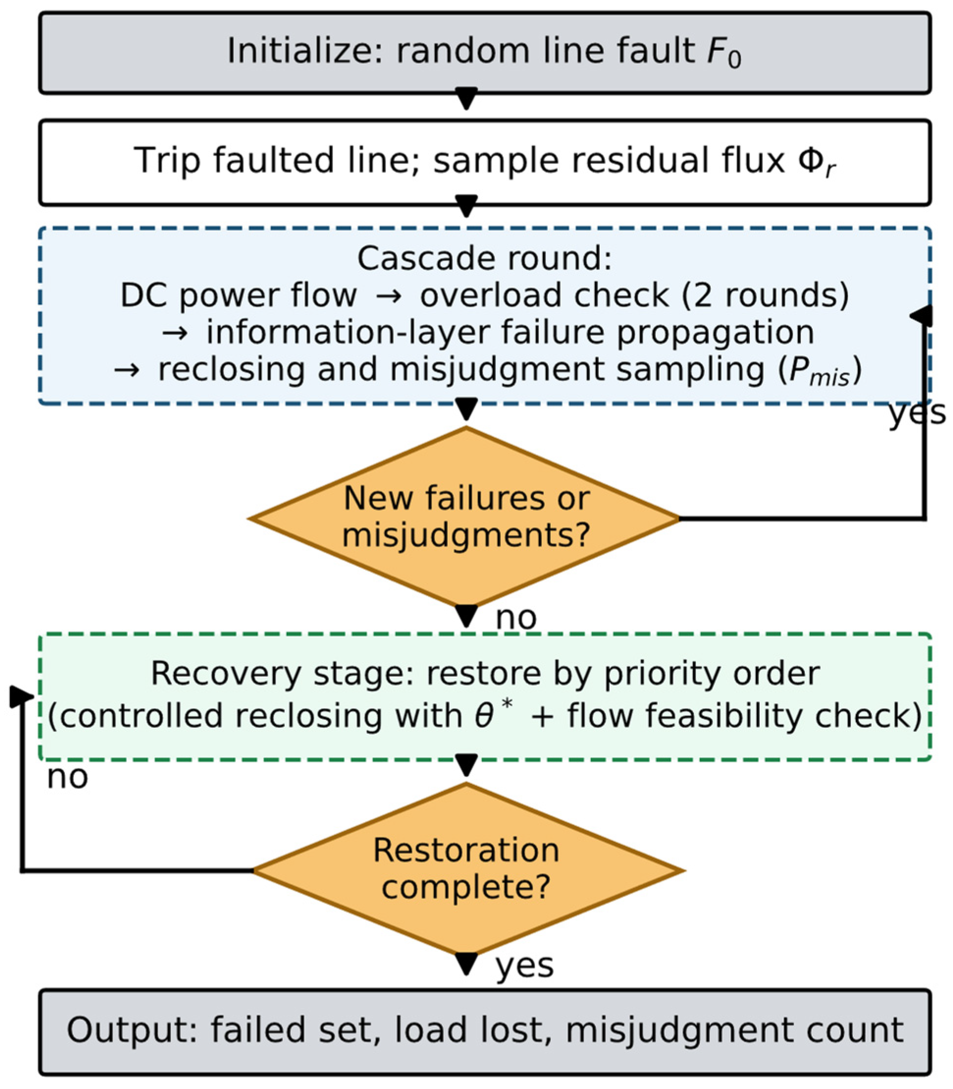
The cascading propagation process proceeds in discrete rounds, each including: power-flow calculation → overload determination and tripping (T1) → information-layer failure propagation (T4) → reclosing event sampling (closing angles generated by the strategy or from a uniform distribution) → misjudgment sampling (T2) → out-of-control determination (T3). The process terminates when no new state change occurs or the maximum number of rounds is reached. The same initial fault set is repeated N times (N = 2000 in this paper) to statistically characterize the randomness of cascading outcomes. The algorithm flow is shown in Figure 5.
Figure 5.
Flowchart of the Monte Carlo simulation of the cascading propagation process.
The fault-state reachability of node is defined as the frequency with which node ends in a faulty or out-of-control state among the cascading simulations:
Unlike static topological indices such as betweenness centrality and node degree [20,21,22], is dynamically generated by the complete propagation process incorporating the electromagnetic mechanism, and thus encodes the topological position, the power-flow distribution, and the inrush trigger mechanism simultaneously. It can therefore identify hidden critical nodes that are topologically inconspicuous but highly vulnerable to misjudgment breakdown under unfavorable residual-flux–closing-angle conditions. The computation of only requires adding counters in the propagation simulation and introduces almost no additional computational cost.
2.5. Adaptive Reclosing Recovery Control Strategy Based on Node Fault-State Reachability
2.5.1. Physical Side: Residual-Flux Prediction and Optimal Closing-Angle Selection
Given the predicted residual flux , the optimal closing angle follows from Equation (7):
From the explicit structure of Equation (7), when cos , i.e., closing at the peak of the phase voltage, the bias flux is minimized; thus in the single-phase sense . When the three phases are coordinated, the phase constraints of the three-phase inrush peaks must be considered simultaneously, and this paper optimizes the three phases jointly with the objective of minimizing the maximum phase inrush peak (a small-dimension grid search suffices, with negligible computation) [27,28,29,30,31]. The residual-flux prediction is estimated online from the voltage integral before tripping, combined with the inverse J–A model (see Appendix A for details).
2.5.2. Recovery Ranking and Overall Strategy Flow
When multiple nodes are to be restored after a fault, the recovery order is ranked by descending reachability:
That is, the nodes “most frequently involved in cascades” with high reachability are restored first, so that they leave the faulty set as early as possible and the subsequent propagation chain is structurally cut off; the recovery operation simultaneously invokes the controlled switching of Section 2.5.1, avoiding “creating a new inrush trigger source by the recovery itself”. This strategy forms a contrast with conventional recovery in the order of fault occurrence or with fixed priorities (see the ablation in Section 3.4).
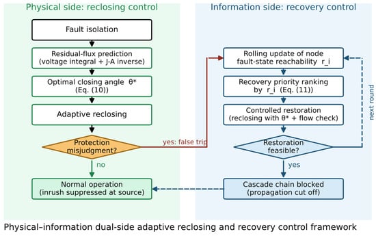
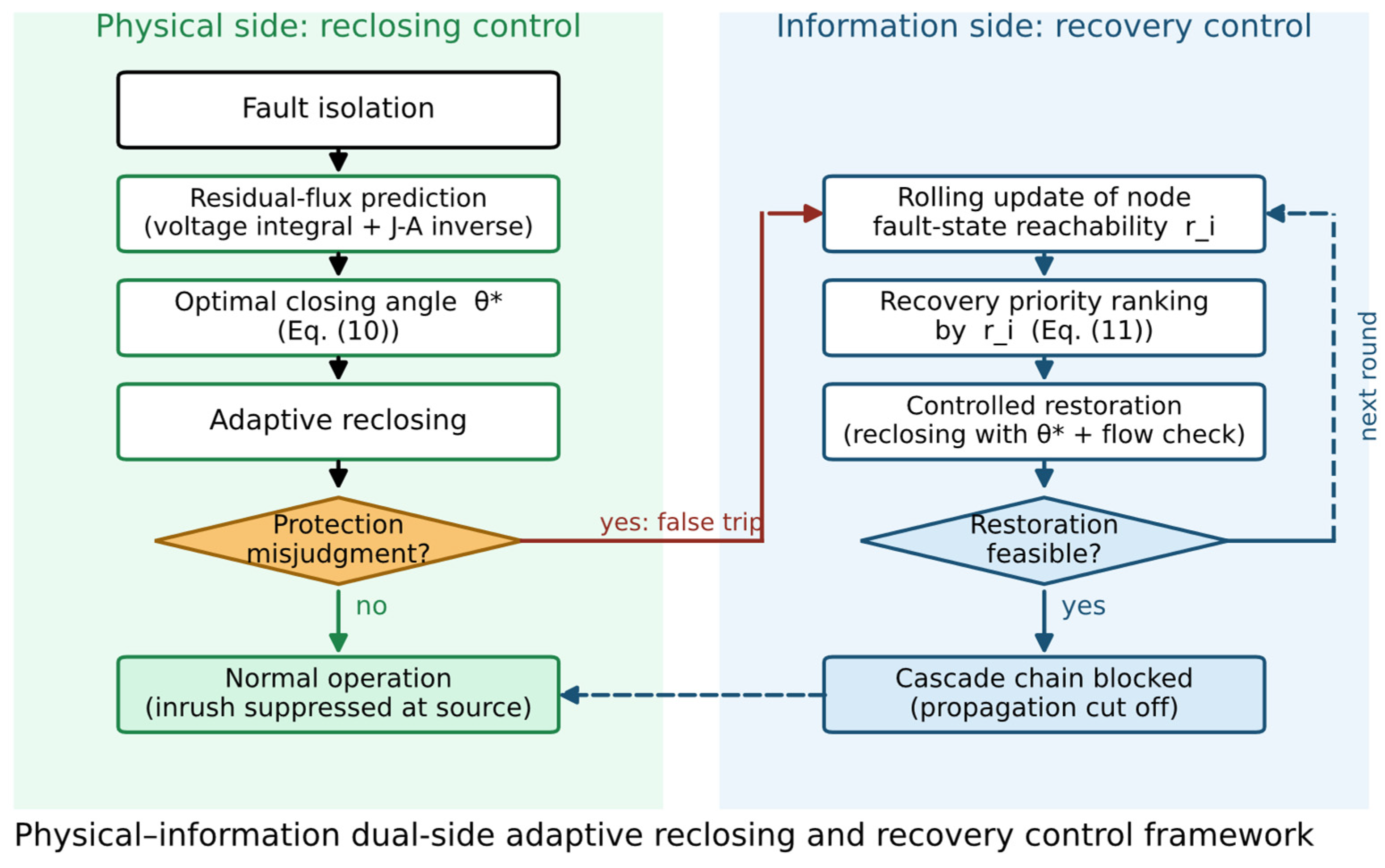
The strategy flow is shown in Figure 6 and consists of three stages:
Figure 6.
Physical–information dual-side adaptive reclosing and recovery control framework.
- (i)
- After fault isolation, the residual flux of each transformer node is predicted;
- (ii)
- The optimal closing angle of each node is determined according to Equation (10) and adaptive reclosing is executed;
- (iii)
- If misjudgment/tripping occurs, the reachability estimate is updated on a rolling basis and recovery is performed according to Equation (11). All stages can be completed within engineering time scales (s).
2.6. Case-Study Settings
The physical grid adopts the standard IEEE 39-bus test system (10 generators, 39 buses), in which the step-up transformer branches (nine in total, i.e., the generator branches) are replaced by the proposed DAE model, while the remaining transformers use conventional models. The information layer corresponds to the substation communication structure, with five additional random links to represent information redundancy. The simulation platform is MATLAB R2021a with Simulink, cross-validated by a Python 3.12 simulation chain developed by the authors: the electromagnetic transient of a single transformer is solved by numerical integfiration of the DAE, and the system-level power flow and cascading process are driven by a self-developed program; the differential protection criterion is implemented as ratio differential plus second-harmonic restraint. The initial fault is a transient fault on a randomly selected line; the information layer IED failure rate is 0.15; the loading level is 1.12 times the base state; the line limit is 1.35 times the base power flow plus 10 MW; the differential pickup is 0.8 × ; and the second-harmonic restraint threshold is 15%. The main parameters are listed in Table 1.
Table 1.
Main simulation parameters.
The information layer is generated as follows: each substation bus is mapped one-to-one to an IED node, and five additional links are added between randomly selected IED pairs, giving the adjacency structure of Gc; an IED fails with probability 0.15 per round (information-layer attack intensity), and a failed IED causes a false tripping of an adjacent healthy branch with probability pe = 0.2. The cascading round terminates when no new failure occurs within a round or after eight rounds; a restoration attempt is accepted only if the post-restoration flow check |Fi| ≤ Fimax passes, with a restoration capacity of two branches per round (up to eight rounds).
3. Results
This section is organized in the order of “model validation → parameter influence → propagation characteristics → control performance → robustness”. Unless otherwise specified, the results are statistical quantities from = 2000 Monte Carlo simulations.
3.1. Validation of the Reclosing Transient Model
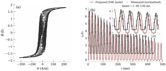
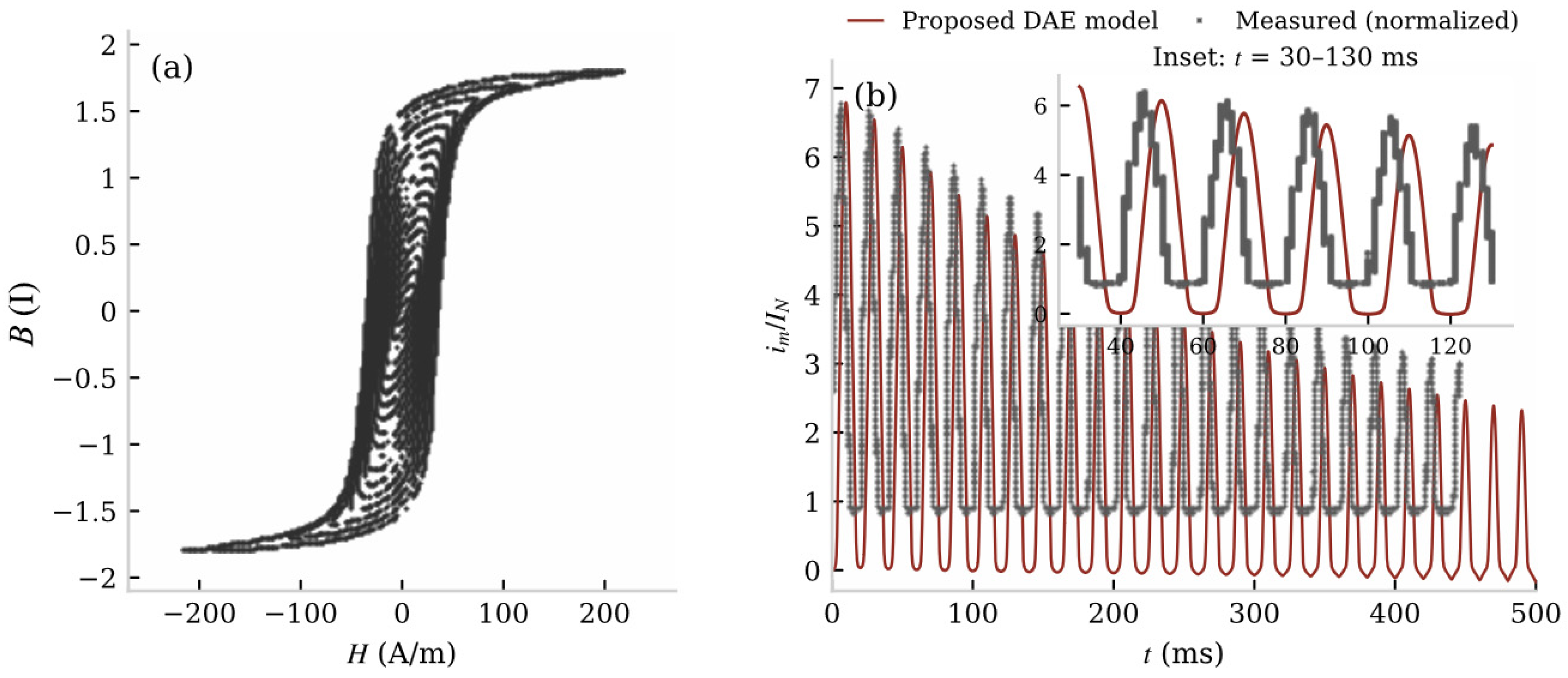
The proposed model is validated against measured data at two levels. Figure 7a shows the measured hysteresis loop family of the transformer core, which is the sample data for identifying the J–A parameters (Ms ≈ 1.43 × 10⁶ A/m, a = 499, α = 7.09 × 10⁻⁴, k = 1154.6, c = 0.0198). Figure 7b compares the inrush current waveform produced by the DAE model with the measured waveform under the same residual flux (+0.8 pu) and closing angle (0°): the two waveforms agree closely, with a peak error of 1.8% and an envelope correlation coefficient of 0.997; The waveform labelled ‘Measured (normalized)’ is the magnetizing current recorded in our previous short-circuit experiment on the short-circuit test model (residual flux +0.8 pu, switching angle 0°), digitized from the measured records and normalized to its own peak for shape comparison; it is a measured transient waveform of the same physical mechanism (bias–residual superposition driving the core into saturation), not a reclosing record; across the whole residual-flux–closing-angle grid of Section 3.2 the peak error does not exceed 10%. The semi-analytical peak estimate of Equation (7) deviates from the DAE numerical result by about 11% on average, with larger deviations near critically saturated conditions.
Figure 7.
(a) Measured hysteresis loop family of the transformer core (sample data for the J–A parameter identification); (b) comparison of the inrush current waveforms from the proposed DAE model and the measurement (residual flux +0.8 pu, closing angle 0°); peak error = 1.8%, envelope correlation coefficient R = 0.997.
Moreover, the J–A field–circuit coupled modeling chain adopted in this paper has been verified against short-circuit tests in our previous study of transformer short-circuit conditions: the errors of the calculated current peaks based on the short-circuit test model (emulating the ODFPS-250000/500 kV product), computed relative to the measured values, range from 5% to 22%, and the largest error occurs at the deepest saturation, consistent with the trend of Equation (7) that “the deeper the saturation, the stronger the nonlinearity”; the finite-element calculated values of the product-level leakage flux agree with the measurements at the mid-height of the winding. These prior verifications support the credibility of the modeling chain from the side. We clarify the scope of this indirect validation: the short-circuit tests verify the credibility of the J-A field–circuit coupled solution chain, while the direct validation of the reclosing transient rests on the waveform comparison of Figure 7b; validation against measured reclosing records remains future work.
3.2. Influence of Residual Flux and Closing Angle on the Inrush Characteristics
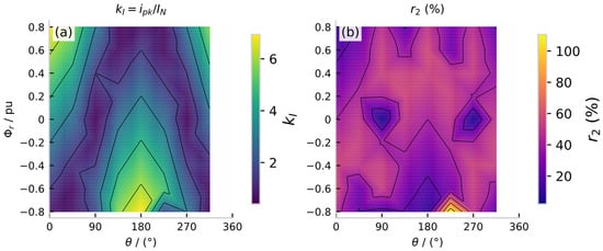
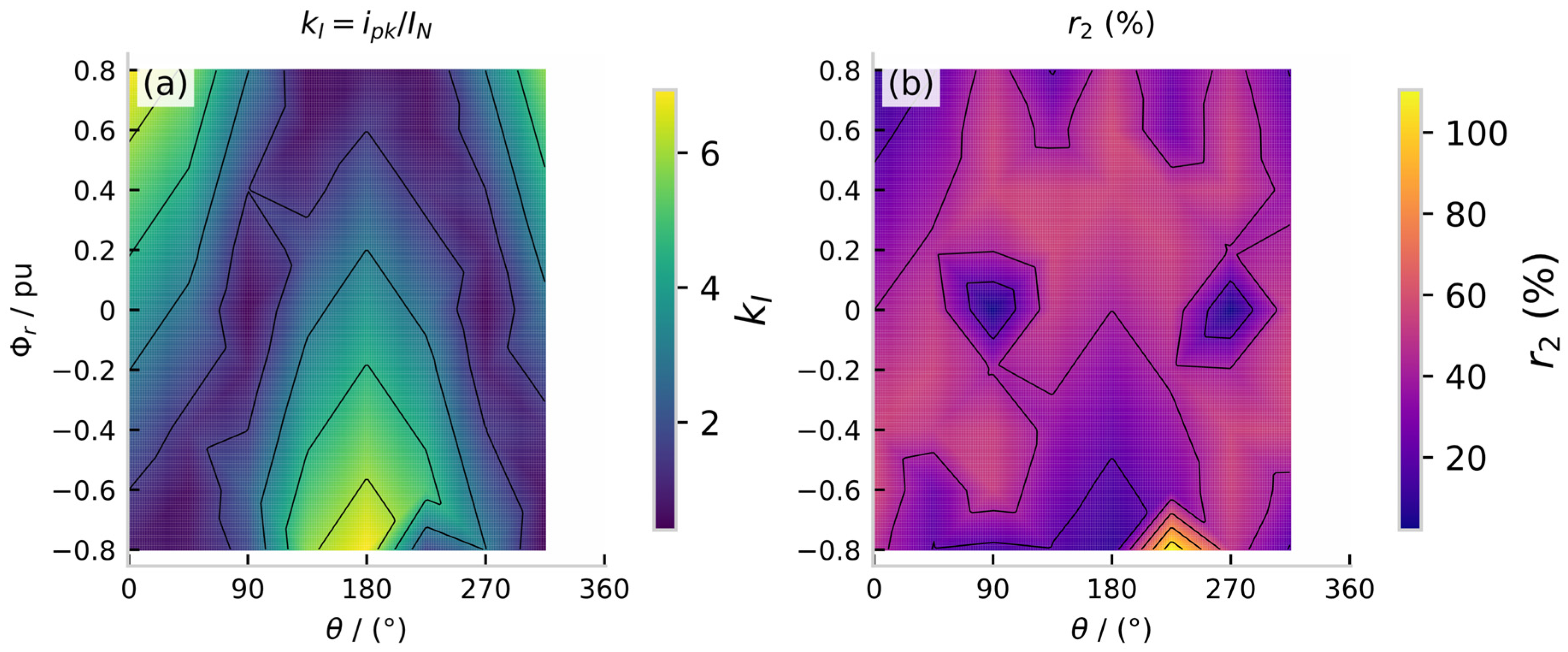
Figure 8a,b show the peak multiple and the second-harmonic ratio over the residual-flux–closing-angle plane. It can be seen that (i) grows approximately linearly with , consistent with Equation (7); (ii) decreases significantly as increases and the closing angle deteriorates; in the region where the residual flux and closing angle superimpose with the same polarity ( and within ±45° of 0°/180°), falls below the second-harmonic restraint threshold (15%), and the misjudgment risk rises sharply. The shape and location of this “high-risk region” are determined by the hysteresis parameters and cannot be reproduced by simplified magnetization models; they also directly determine the calibration range of the coefficients in the misjudgment probability model of Section 2.3.
Figure 8.
Distribution of the inrush features over the residual-flux–closing-angle plane: (a) peak multiple ; (b) second-harmonic ratio .
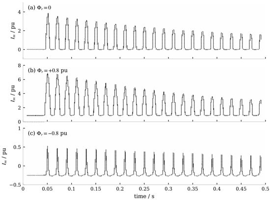
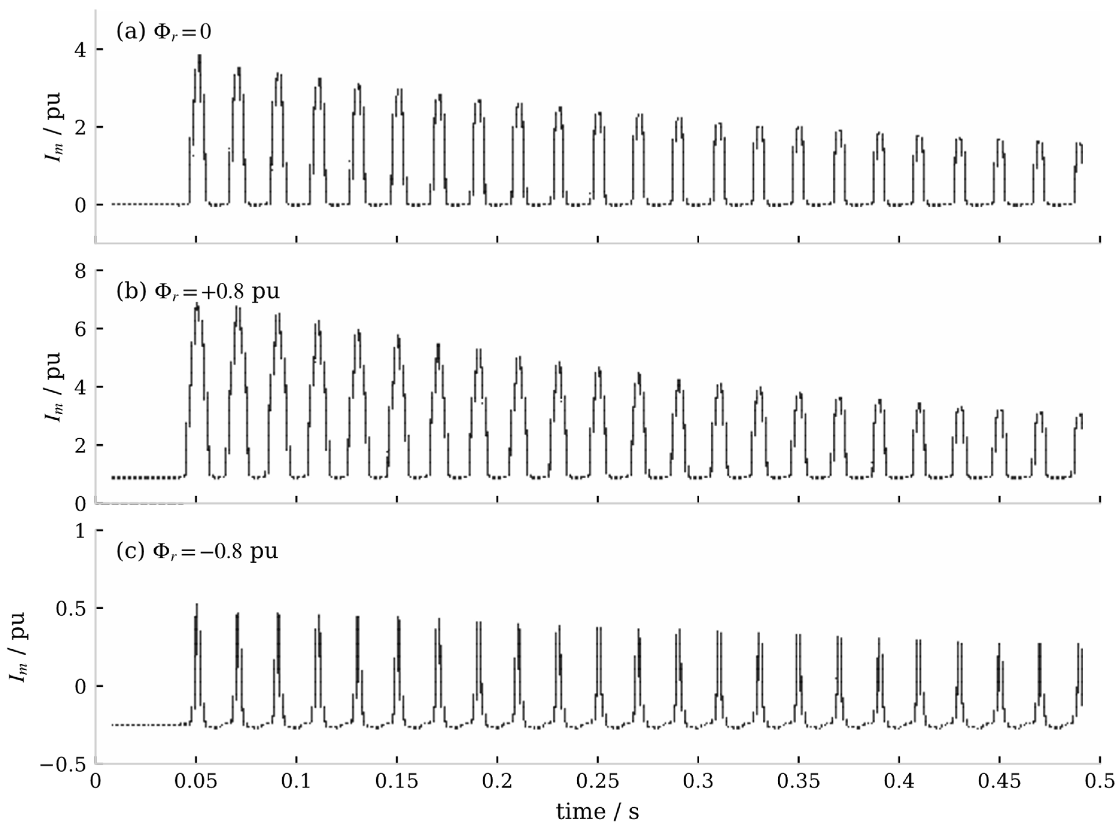
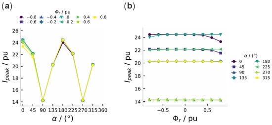
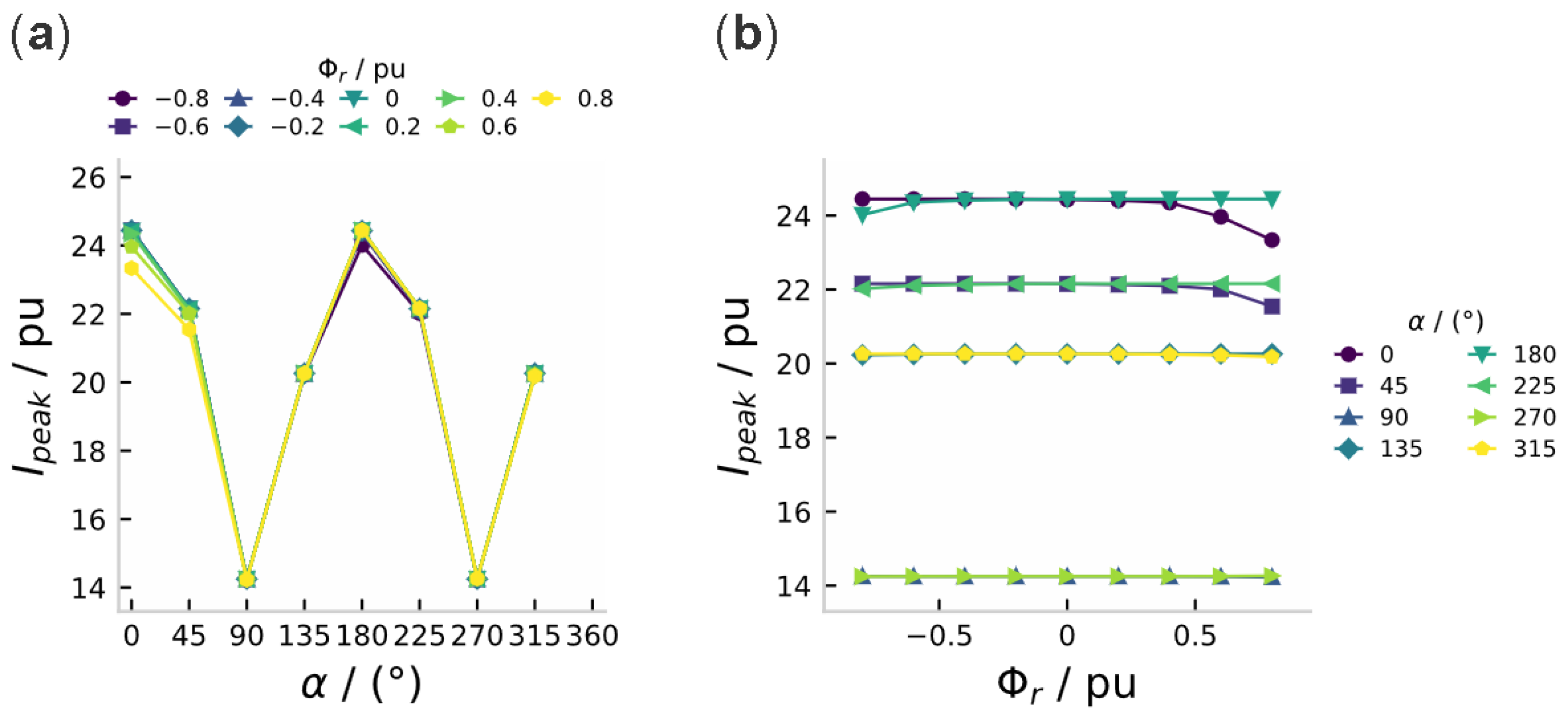
As shown in Figure 9, when the residual flux has the same polarity as the bias flux, the amplitude of the magnetizing current increases significantly (peak of about 6.9 ), whereas the two cancel each other out under opposite polarity (peak below 1 ). In addition, the sensitivity law of “high sensitivity to the phase angle, with the residual flux being secondary but non-negligible” is consistent with our previous results on transformer short-circuit conditions: as shown in Figure 10, the first peak of the short-circuit current varies greatly with the switching angle (14.25–24.45 ), while the residual flux introduces a correction of only about 5%. This indicates that the mechanism of “bias–residual superposition causing core saturation” is universal under different transient conditions, which indirectly supports the reasonableness of introducing this mechanism into the cascading trigger modeling.
Figure 9.
Transformer excitation current waveforms under different residual flux (switching angle α = 0°): (a) = 0; (b) = +0.8 ; (c) = −0.8 .
Figure 10.
First peak of the short-circuit current versus the switching angle and residual flux (results from the prior equivalent-circuit analytical model): (a) peak–angle characteristics parameterized by residual flux; (b) peak–remanence characteristics parameterized by switching angle.
The near-coincidence of the residual-flux-parameterized curves in Figure 10a and the flatness of the α = 0°/180° curves in Figure 10b quantify the same law from two viewpoints: the closing angle dominates the first peak (14.25–24.45 pu) while the residual flux contributes a correction of only about 5%, and the separation is visible only where the two effects compete (α near 0°/180°).
3.3. Misjudgment Probability and Cascading Propagation Characteristics
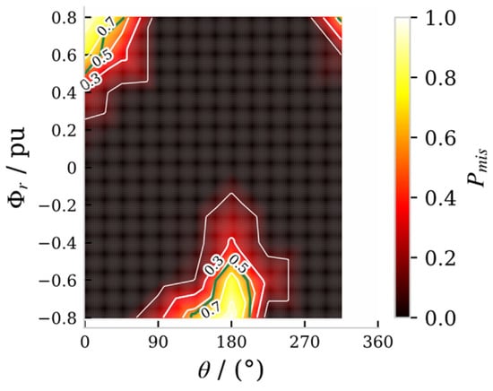
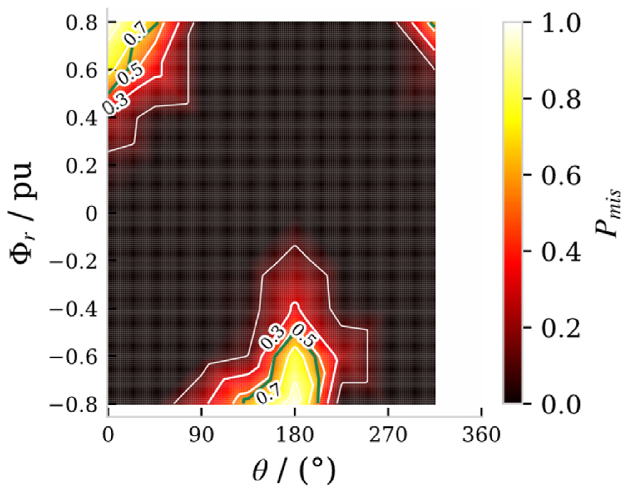
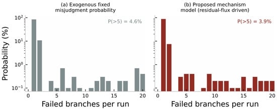
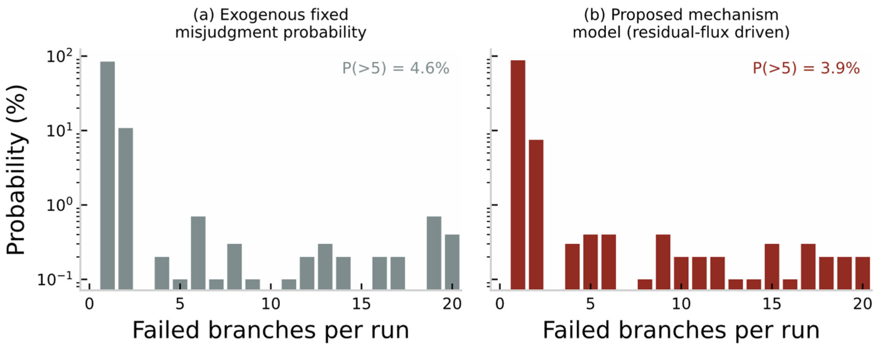
Figure 11 shows the distribution of the misjudgment probability of Equation (8) over the residual-flux–closing-angle plane. The high-risk region is consistent with the inrush feature analysis of Section 3.2, which validates the selected features. Figure 12 compares the cascade size distributions under two trigger settings (N = 1000 Monte Carlo runs): (a) the idealized model with an exogenous fixed misjudgment probability (calibrated to the average trigger rate of the mechanism model); (b) the proposed mechanism model. Both models exhibit long-tailed distributions, but the triggers of the mechanism model concentrate in the physically explainable region of unfavorable residual-flux–closing-angle superposition (Figure 8), and the trigger sources of large-cascade events can be quantitatively traced back to the residual flux and closing angle, which the idealized exogenous model cannot provide.
Figure 11.
Distribution of the protection misjudgment probability over the residual-flux–closing-angle plane (white contours: simulated values; green line: the 0.5 boundary of the logistic model).
Figure 12.
Comparison of the cascade-size distributions under two trigger settings (N = 1000 Monte Carlo runs).
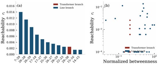
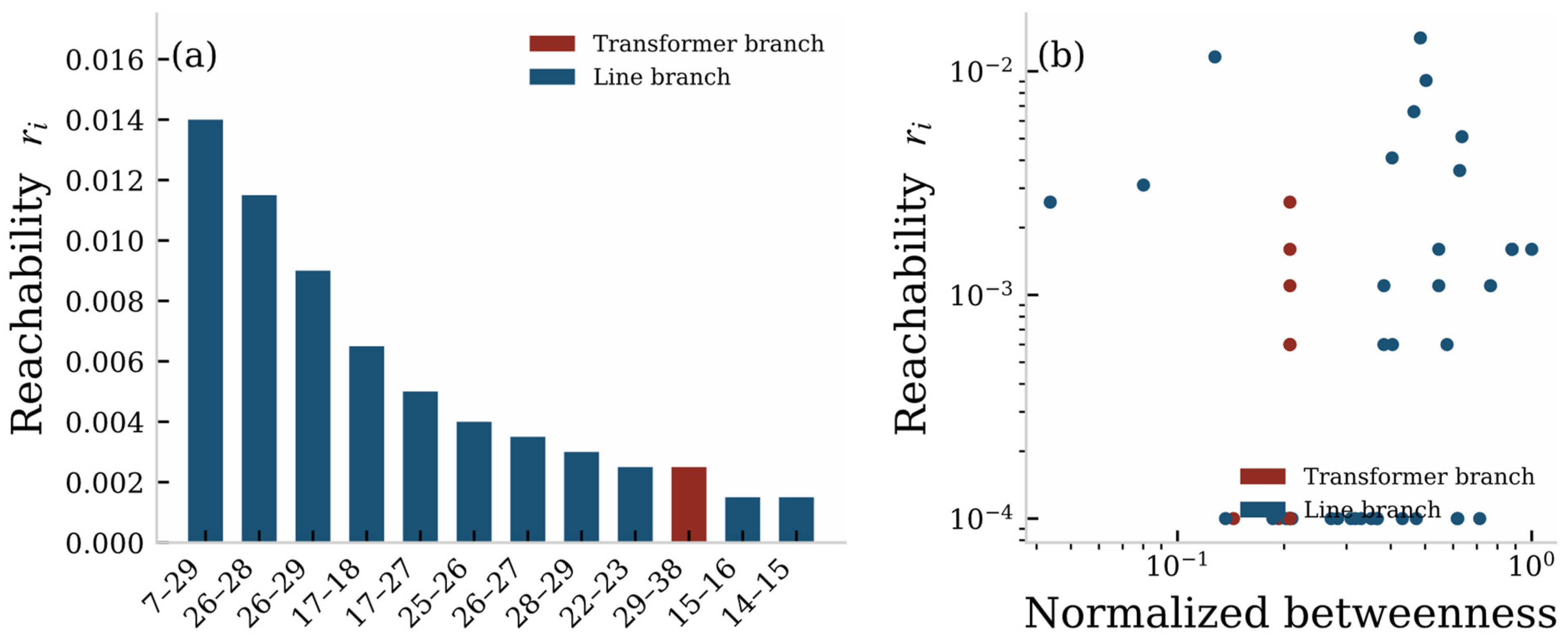
Figure 13 shows the ranking of the reachability of selected branches and its comparison with betweenness centrality [20,21]. Branch 17–18 ranks first in reachability (r = 0.052), while its betweenness centrality ranks only 16th out of 47: this branch lies in a critical corridor of the cascading propagation, which static topological indices cannot reflect. This difference demonstrates the identification capability of the reachability index that incorporates the electromagnetic mechanism.
Figure 13.
Branch fault-state reachability: (a) ranking of reachability (red: transformer branches); (b) reachability versus betweenness centrality.
3.4. Performance Comparison of Recovery Control Strategies
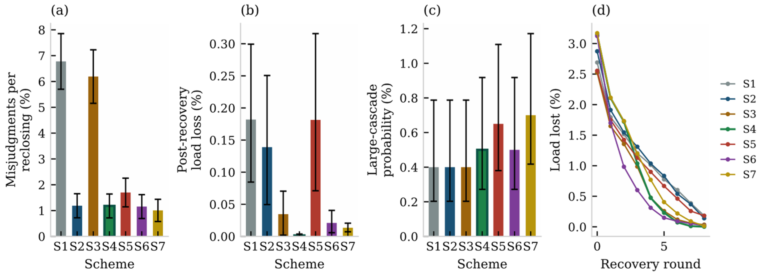
Four schemes are compared first: S1, conventional fixed time-delay reclosing with recovery in the order of fault occurrence; S2, controlled switching only (Section 2.5.1); S3, reachability-based recovery ranking only (Section 2.5.2); and S4, the proposed dual-side coordinated strategy. To isolate the effect of the recovery ranking, three additional schemes with identical settings except the recovery order are included: S5, controlled switching with random recovery order; S6, controlled switching with recovery ranked by betweenness centrality; and S7, controlled switching with recovery ranked by the amount of load restored per branch. Because large cascades are rare, misjudgments per reclosing operation and the post-recovery load loss, which are accumulated over thousands of reclosing events, are used as the primary metrics, together with the large-cascade probability and its 95% confidence interval. The results are given in Table 2 and Figure 14.
Table 2.
Performance comparison of the seven schemes (2000 Monte Carlo runs per scheme; values in parentheses are 95% confidence intervals; CS: controlled switching).
Figure 14.
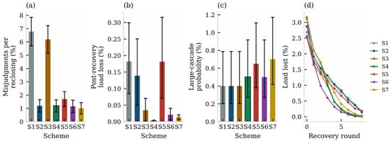
Performance comparison of the seven schemes: (a) misjudgments per reclosing operation with 95% confidence intervals; (b) post-recovery load loss with 95% CIs; (c) large-cascade probability with 95% CIs; (d) load recovery curves.
- (1)
- The misjudgment rate drops from 6.78% (95% CI: 5.71–7.86%) in S1 to 1.18% (0.72–1.64%) in S4—a reduction of about 83%; S2 and S4 achieve the same rate (1.19% and 1.18%), showing that the misjudgment rate is governed by the controlled switching and that the recovery ranking introduces no additional misjudgment risk (restoration reclosings also use θ*); the difference between the misjudgment counts reported in the previous version was due to sampling fluctuation.
- (2)
- The post-recovery load loss is reduced from 0.182% (95% CI: 0.085–0.299%) in S1 to 0.001% (0–0.004%) in S4. Under identical controlled switching, the ordering matters: random order (S5, 0.181%) gives no benefit at all, while betweenness (S6, 0.021%) and load-based (S7, 0.013%) orders give intermediate benefits; the reachability ranking achieves the largest reduction and its confidence interval is separated from all three ordering baselines under identical controlled switching (S5–S7), which justifies the index; the overlap with S3 is expected, since S3 does not include controlled switching and therefore suffers a much higher misjudgment rate—this contrast is itself part of the evidence for the dual-side design.
- (3)
- S2 alone leaves the load loss at 0.139% because it cannot block already-formed propagation chains, and S3 alone leaves the misjudgment rate at 6.19% because the “first domino” still falls; only S4 optimizes both, verifying the necessity of dual-side coordination.
- (4)
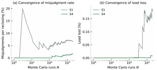
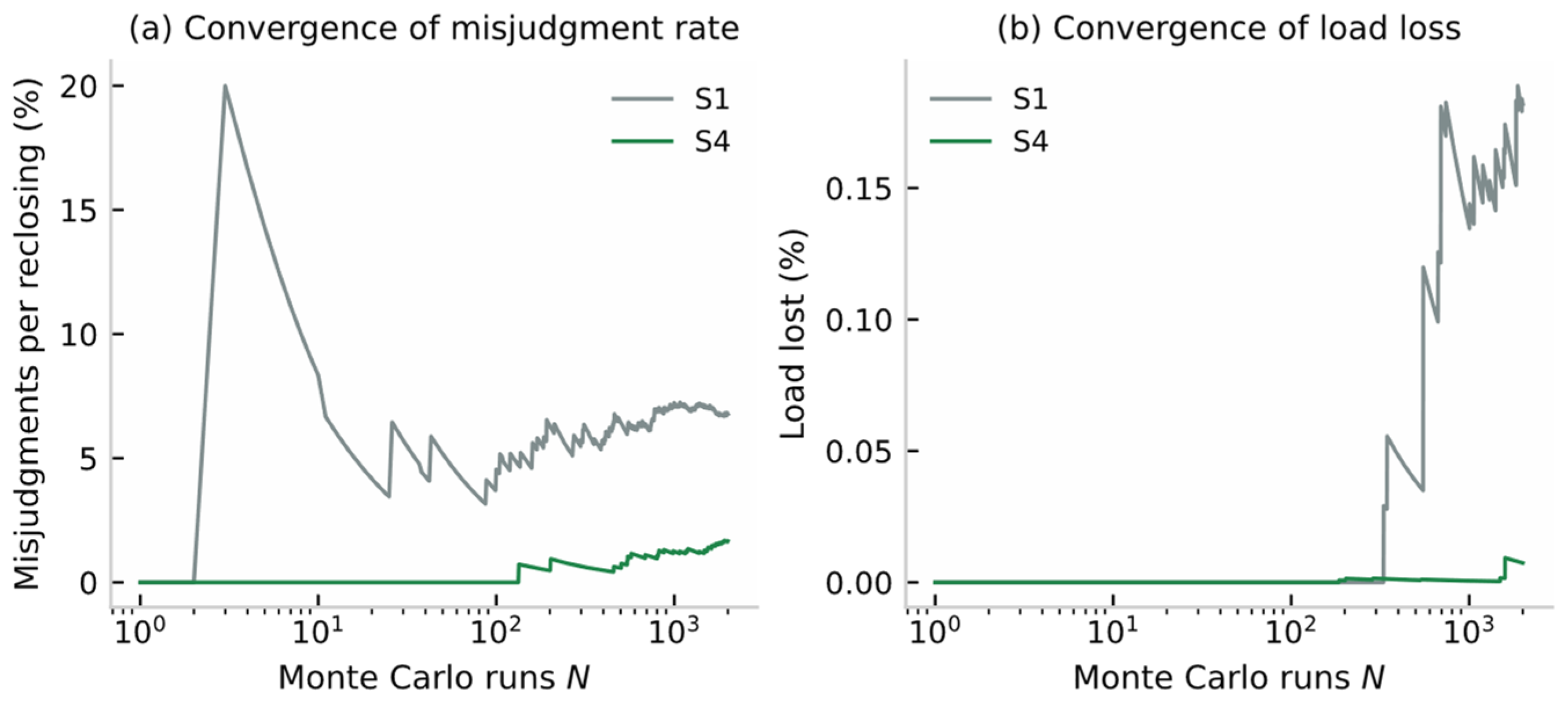
- The large-cascade probability is 0.4–0.5% for S1/S2/S3/S4 with overlapping confidence intervals: with only 8–10 events per 2000 runs this metric cannot resolve the schemes, and we therefore do not claim a significant difference here; the Monte Carlo convergence of the principal metrics is shown below, where the misjudgment rate stabilizes to within ±10% of its final value after about 500 runs, whereas the load loss—driven by rare large cascades—converges more slowly and requires roughly 1500–2000 runs, which motivates the choice of N = 2000. The final values of Figure 16 agree with Table 2 (S1: 6.78% and 0.182%; S4: 1.18% and 0.001%), as both derive from the same simulation program with identical settings, with the convergence pass being a separately seeded run of the same chain.
3.5. Robustness Analysis
Sensitivity analyses are carried out:
- (i)
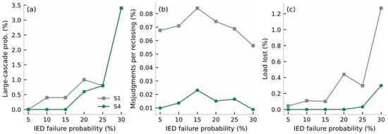
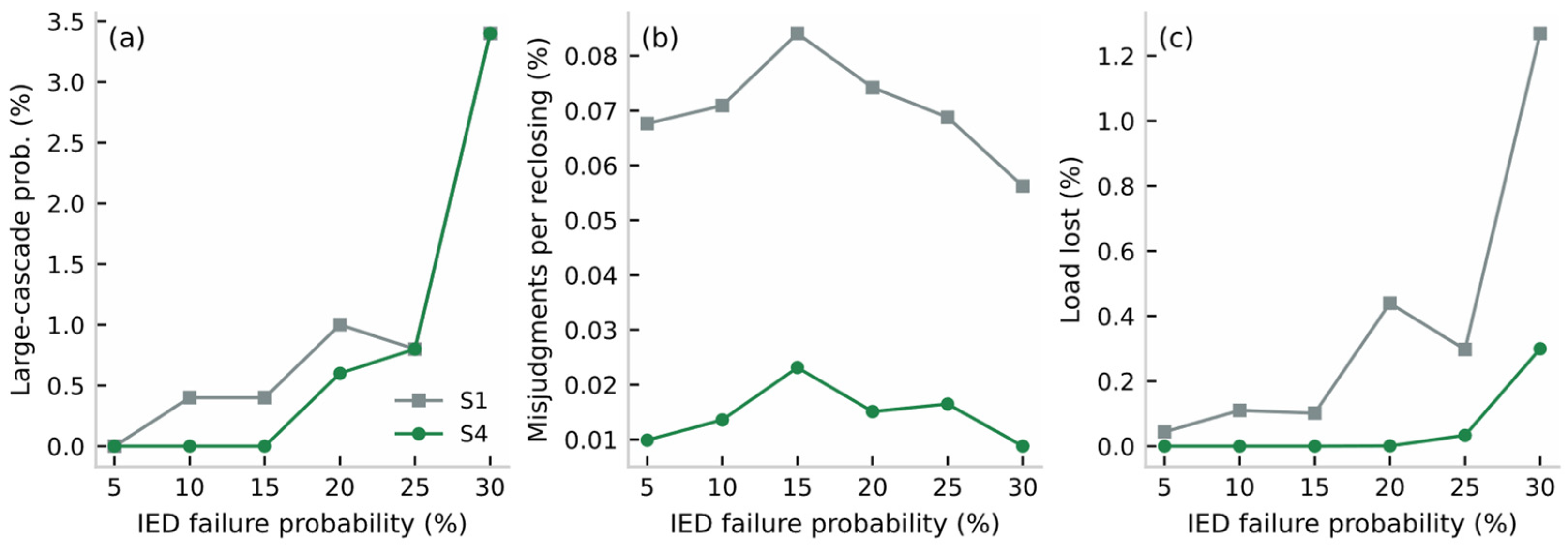
- Information-layer attack-intensity sweep (IED failure rate from 5% to 30%, 500 runs per point): the misjudgment rate of S4 stays below 2.3% over the whole range (versus 5.6–8.4% for S1), and its large-cascade probability is no higher than that of S1 at every intensity;
- (ii)
- The conclusions are robust to the initial fault location (random line faults);
- (iii)
- Perturbing the coefficients β of the misjudgment model by ±20% does not change the relative ranking of the schemes. The 15% point of Figure 15 is obtained with 500 runs per point, whereas Table 2 uses 2000 runs; the absolute values therefore differ slightly, but the ordering (S4 no worse than S1) is preserved in both cases for the misjudgment rate and the load loss; for the large-cascade probability, the 15% point of Table 2 shows S4 (0.5%) slightly above S1 (0.4%), but the difference is well within the overlapping confidence intervals and is not claimed as significant. Figure 16 further shows the Monte Carlo convergence of the principal metrics.Figure 15. Robustness against information-layer attack intensity (S1 vs. S4): (a) large-cascade probability; (b) misjudgments per reclosing operation; (c) post-recovery load loss (500 runs per point).Figure 16. Monte Carlo convergence of (a) the misjudgment rate per reclosing operation and (b) the post-recovery load loss for S1 and S4.
4. Discussion
4.1. Mechanistic Implications of the Results
The results in Section 3.2 and Section 3.3 quantitatively confirm the central argument of this paper: the triggering of cascading failures is not uniformly random but concentrates in a physically explainable region composed of unfavorable residual-flux–closing-angle combinations. This means that cascading defense has a clear time window and physical lever: before reclosing occurs, the trigger probability can be greatly reduced by residual-flux prediction and controlled switching [27,28,29,30]; once triggered, the reachability ranking on the information side can cut off the “leverage nodes” early in the propagation. The ablation results of S2/S3 in Section 3.4 show that neither side alone can simultaneously suppress the trigger rate and the propagation scale, which argues from the opposite side for the necessity of physical–information dual-side coordination and echoes the mutual causality of “maloperation” and “propagation” in major blackout accidents [1,2,18,19].
Three observations from the figures deserve further interpretation.
- (a)
- Figure 8 shows that the region where r2 falls below the 15% restraint threshold forms two bands symmetric about θ = 0°/180° in the (θ, Φr) plane; this mirrors the cos θ dependence of the bias flux in Equation (6) and explains why the misjudgment probability map of Figure 11 exhibits the same lobed structure—the protection risk is a direct image of the electromagnetic mechanism.
- (b)
- Figure 12 shows that although both trigger settings produce long-tailed cascade-size distributions, the tail of the mechanism model is fed exclusively by the unfavorable residual-flux–closing-angle region of Figure 11, whereas the exogenous model spreads its triggers uniformly and cannot support source tracing; this is the practical value of the mechanistic trigger.
- (c)
- Figure 14a shows that the misjudgment rate is insensitive to the recovery policy (S1 vs. S3; S2 vs. S4), whereas Figure 14b shows that the load loss is insensitive to the switching policy (S1 vs. S2) but strongly depends on the recovery ordering (S5 vs. S6/S7 vs. S4); the two panels together justify the dual-side design—each side governs one metric, and only their combination optimizes both.
4.2. Differences from Existing Studies
Compared with complex-network-based cascading models [20,21,22,23], the trigger mechanism of this paper is endogenous to the electromagnetic transient model, and the misjudgment probability varies with operating conditions instead of being an exogenous constant. Compared with pure controlled switching studies [27,28,29,30], this paper evaluates inrush suppression in the overall framework of cascading failure defense, showing that the value of controlled switching lies not only in protecting the local transformer but also in weakening the system-wide cascading trigger source. Compared with conventional recovery control [24,25,26], the reachability index is dynamically generated by the mechanistic propagation process and can identify hidden critical nodes masked by topological indices. Recent comprehensive reviews [32,33] corroborate the need for such mechanistic trigger models.
4.3. Engineering Applicability and Limitations
In terms of engineering applicability: the J–A parameters can be identified from conventional no-load tests [14,15,16,17]; controlled switching devices are mature in engineering practice [27,28]; the reachability computation only requires adding statistical counters to existing dispatching/simulation platforms, and the implementation cost is low. The limitations of this paper include: (i) static power flow and deterministic overload criteria are adopted, without considering transient stability constraints; (ii) the information-layer topology and failure model are simplified, and targeted attacks and information delays are not modeled [5,6,7,8]; (iii) the validation is simulation-based, supported by measured short-circuit waveforms, and lacks calibration against measured reclosing records; (iv) the quasi-static matching of the J–A loops to the measured family of grain-oriented steel is less accurate than the transient matching of Figure 7b, and a modified Langevin or Preisach constitutive model could further improve the static fidelity. Recent reviews on CPPS resilience metrics and modeling [34] provide further engineering context.
4.4. Future Work
Future work will proceed in three directions: first, the interaction of residual magnetism and the superposition of inrush currents under simultaneous reclosing of multiple transformers; second, data-driven calibration of the J–A parameters and the misjudgment probability model using measured fault recordings; third, explicitly incorporating information-layer attacks (false data injection, delay attacks) into the propagation model [6,7] to study defense under coordinated physical–information attacks. Moreover, extending the proposed framework to inverter-dominated grids, where inrush mitigation faces new constraints [35], is a promising direction.
5. Conclusions
This paper addresses the problem of cascading failures induced by transformer reclosing inrush in CPPS and establishes a complete analytical modeling chain of “physical transient—information misjudgment—propagation dynamics—recovery control”. The main conclusions are as follows:
- (1)
- A DAE-based transient model of three-phase transformer reclosing is established based on the J–A theory, in which the residual magnetism naturally enters the closing initial condition as a hysteresis-loop property, and semi-analytical expressions of the inrush peak, harmonic characteristics, and decay law with respect to the residual flux and closing angle are derived; simulation verification shows that the model accurately reproduces the quantitative influence of hysteresis residual magnetism on the inrush characteristics.
- (2)
- An inrush-feature-driven misjudgment probability model and a cascading propagation model incorporating physical–information state transitions are constructed, and the node fault-state reachability index is proposed, which can identify hidden critical nodes that topological indices cannot discover.
- (3)
- An adaptive reclosing recovery control strategy based on reachability is proposed, which suppresses the inrush at the source through residual-flux prediction and optimal closing-angle selection and blocks the propagation chain by prioritizing the recovery of high-reachability nodes. IEEE 39-bus simulations show that, compared with the conventional reclosing scheme, the misjudgment rate per reclosing operation is reduced from 6.78% to 1.18% (approximately 83%) and the post-recovery load loss from 0.182% to 0.001%, and that the reachability-based recovery ranking outperforms random, betweenness-based, and load-based orderings under identical conditions.
The proposed framework provides a new idea for the mechanistic modeling and coordinated prevention and control of cascading failures in CPPS, and is also of reference value for the reclosing control of power grids with a high penetration of power electronic equipment.
Author Contributions
Conceptualization, Y.Z. and B.Z.; methodology, Y.Z. and X.H.; software, J.L. and Q.Z.; validation, J.L. and Q.Z.; formal analysis, Y.Z.; investigation, X.Z.; writing—original draft preparation, Y.Z.; writing—review and editing, B.Z. and X.Y.; supervision, B.Z.; project administration, Y.Z.; funding acquisition, Y.Z. All authors have read and agreed to the published version of the manuscript.
Funding
This research was funded by the Basic Scientific Research Project of the Education Department of Liaoning Province (LJ212411632070), “Research on Cascading Failure Propagation and Control Models in Cyber-Physical Power Systems”.
Data Availability Statement
The simulation data and code are available from the corresponding author upon reasonable request.
Conflicts of Interest
The authors declare no conflicts of interest. The funders had no role in the design of the study; in the collection, analyses, or interpretation of data; in the writing of the manuscript; or in the decision to publish the results.
Abbreviations
| CPPS | Cyber-Physical Power System |
| DAE | Differential-Algebraic Equation |
| J–A | Jiles–Atherton (hysteresis model) |
| EMT | Electromagnetic Transient |
| CT | Current Transformer |
| IED | Intelligent Electronic Device |
Appendix A
Appendix A.1. Parameter Identification of the J–A Model
Using the no-load current–voltage curve of the transformer measured from the no-load test, combined with the magnetization data of the core material, the five J–A parameters () are identified by the particle swarm optimization algorithm, with the objective of minimizing the relative deviation between the areas enclosed by the measured and modeled hysteresis loops [15,16,17]. The identified parameters are: , , , , and , corresponding to a saturation flux density of about 1.8 T and a residual flux of about 0.68 T, which agree with the measured hysteresis loop (Figure 7).
Appendix A.2. Online Residual-Flux Estimation and Derivation of Equation (7)
After tripping, the winding is open-circuited and the flux decays naturally along the J–A loop to the residual point. The residual flux can be obtained by integrating the voltage before tripping to obtain the initial flux linkage and then numerically integrating along the descending branch of the loop, without additional sensors [29]. The derivation of Equation (7) is briefly as follows: after saturation, the equivalent inductance of the magnetizing branch is approximately constant, and the inrush peak corresponds to the part by which the peak flux exceeds the saturation flux ; from the inductance definition i = N1(Φ − Φs)/L0, Equation (7) follows (the detailed derivation is omitted).
Appendix A.3. Experimental Verification of the Modeling Chain
Table A1.
Comparison of measured and calculated peak values of the short-circuit test model currents (prior experimental results).
References
- De La Ree, J.; Liu, Y.; Mili, L.; Phadke, A.G.; Das, R. Catastrophic failures in power systems: Causes, analyses, and countermeasures. Proc. IEEE 2005, 93, 907–921. [Google Scholar] [CrossRef] [Scilit]
- Chen, J.; Thorp, J.S.; Dobson, I. Cascading dynamics and mitigation assessment in power system disturbances via a hidden failure model. Int. J. Electr. Power Energy Syst. 2005, 27, 626–633. [Google Scholar] [CrossRef] [Scilit]
- Yang, Y.; Nishikawa, T.; Motter, A.E. Small vulnerable sets determine large network cascades in power grids. Science 2017, 358, eaan3184. [Google Scholar] [CrossRef] [Scilit] [PubMed]
- Islam, M.Z.; Lin, Y.; Vokkarane, V.M.; Venkataramanan, V. Cyber-physical cascading failure and resilience of power grid: A comprehensive review. Front. Energy Res. 2023, 11, 1095303. [Google Scholar] [CrossRef] [Scilit]
- Huang, Z.; Wang, C.; Stojmenovic, M.; Nayak, A. Characterization of cascading failures in interdependent cyber-physical systems. IEEE Trans. Comput. 2015, 64, 2158–2168. [Google Scholar] [CrossRef] [Scilit]
- Zhang, Y.; Yağan, O. Robustness of interdependent cyber-physical systems against cascading failures. IEEE Trans. Autom. Control 2020, 65, 711–726. [Google Scholar] [CrossRef] [Scilit]
- Gharebaghi, S.; Chaudhuri, N.R.; He, T.; La Porta, T. Dynamic modeling and mitigation of cascading failures in power grids with interdependent cyber and physical layers. IEEE Trans. Smart Grid 2024, 15, 3235–3247. [Google Scholar] [CrossRef] [Scilit]
- Guo, H.; Yu, S.S.; Iu, H.H.C.; Fernando, T.; Zheng, C. A complex network theory analytical approach to power system cascading failure—From a cyber-physical perspective. Chaos 2019, 29, 053111. [Google Scholar] [CrossRef] [Scilit] [PubMed]
- Hamilton, R. Analysis of transformer inrush current and comparison of harmonic restraint methods in transformer protection. IEEE Trans. Ind. Appl. 2013, 49, 1890–1899. [Google Scholar] [CrossRef] [Scilit]
- Weng, H.; Lin, X. Studies on the unusual maloperation of transformer differential protection during the nonlinear load switch-in. IEEE Trans. Power Deliv. 2009, 24, 1824–1831. [Google Scholar] [CrossRef] [Scilit]
- Qi, X.; Yin, X.; Zhang, Z.; Chen, D.; Wang, Y.; Cai, F. Study on the unusual misoperation of differential protection during transformer energization and its countermeasure. IEEE Trans. Power Deliv. 2016, 31, 1998–2007. [Google Scholar] [CrossRef] [Scilit]
- Hodder, S.; Kasztenny, B.; Fischer, N.; Xia, Y. Low second-harmonic content in transformer inrush currents—Analysis and practical solutions for protection security. In Proceedings of the 2014 67th Annual Conference for Protective Relay Engineers, College Station, TX, USA, 31 March–3 April 2014; pp. 705–722. [Google Scholar] [CrossRef] [Scilit]
- Wang, X.; Thomas, D.W.P.; Sumner, M.; Paul, J.; Cabral, S.H.L. Characteristics of Jiles–Atherton model parameters and their application to transformer inrush current simulation. IEEE Trans. Magn. 2008, 44, 340–345. [Google Scholar] [CrossRef] [Scilit]
- Jiles, D.C.; Atherton, D.L. Theory of ferromagnetic hysteresis. J. Magn. Magn. Mater. 1986, 61, 48–60. [Google Scholar] [CrossRef] [Scilit]
- Toman, M.; Stumberger, G.; Dolinar, D. Parameter identification of the Jiles–Atherton hysteresis model using differential evolution. IEEE Trans. Magn. 2008, 44, 1098–1101. [Google Scholar] [CrossRef] [Scilit]
- Zou, M.; Sima, W.; Yang, M.; Li, L.; Yang, Q.; Sun, P. Improved low-frequency transformer model based on Jiles–Atherton hysteresis theory. IET Gener. Transm. Distrib. 2017, 11, 915–923. [Google Scholar] [CrossRef] [Scilit]
- Ren, Y.; Wang, Y.; Liu, C. Low-frequency electromagnetic transient modeling of shell-type transformers based on dynamic Jiles–Atherton hysteresis model. IEEE Trans. Magn. 2024, 60, 7300905. [Google Scholar] [CrossRef] [Scilit]
- Phadke, A.G.; Thorp, J.S. Expose hidden failures to prevent cascading outages. IEEE Comput. Appl. Power 1996, 9, 20–25. [Google Scholar] [CrossRef] [Scilit]
- Tamronglak, S.; Horowitz, S.H.; Phadke, A.G.; Thorp, J.S. Anatomy of power system blackouts: Preventive relaying strategies. IEEE Trans. Power Deliv. 1996, 11, 708–715. [Google Scholar] [CrossRef] [Scilit]
- Pagani, G.A.; Aiello, M. The power grid as a complex network: A survey. Physica A 2013, 392, 2688–2700. [Google Scholar] [CrossRef] [Scilit]
- Liu, B.; Li, Z.; Chen, X.; Huang, Y.; Liu, X. Recognition and vulnerability analysis of key nodes in power grid based on complex network centrality. IEEE Trans. Circuits Syst. II Express Briefs 2018, 65, 346–350. [Google Scholar] [CrossRef] [Scilit]
- Wang, S.; Lv, W.; Zhang, J.; Luan, S.; Chen, C.; Gu, X. Method of power network critical nodes identification and robustness enhancement based on a cooperative framework. Reliab. Eng. Syst. Saf. 2021, 207, 107313. [Google Scholar] [CrossRef] [Scilit]
- Chang, L.; Wu, Z. Performance and reliability of electrical power grids under cascading failures. Int. J. Electr. Power Energy Syst. 2011, 33, 1410–1419. [Google Scholar] [CrossRef] [Scilit]
- Poudel, S.; Dubey, A. Critical load restoration using distributed energy resources for resilient power distribution system. IEEE Trans. Power Syst. 2019, 34, 52–63. [Google Scholar] [CrossRef] [Scilit]
- Gao, H.; Chen, Y.; Xu, Y.; Liu, C.C. Resilience-oriented critical load restoration using microgrids in distribution systems. IEEE Trans. Smart Grid 2016, 7, 2837–2848. [Google Scholar] [CrossRef] [Scilit]
- Liu, Y.; Fan, R.; Terzija, V. Power system restoration: A literature review from 2006 to 2016. J. Mod. Power Syst. Clean Energy 2016, 4, 332–341. [Google Scholar] [CrossRef] [Scilit]
- Brunke, J.H.; Frohlich, K.J. Elimination of transformer inrush currents by controlled switching. I. Theoretical considerations. IEEE Trans. Power Deliv. 2001, 16, 276–280. [Google Scholar] [CrossRef] [Scilit]
- Oliveira, J.C.; Tavares, C.; Apolonio, R.; Vasconcellos, A.; Bronzeado, H. Transformer controlled switching to eliminate inrush current—Part I: Theory and laboratory validation. In Proceedings of the 2006 IEEE/PES Transmission & Distribution Conference and Exposition: Latin America, Caracas, Venezuela, 15–18 August 2006; pp. 1–5. [Google Scholar] [CrossRef] [Scilit]
- Fang, S.; Ni, H.; Lin, H.; Ho, S.L. A novel strategy for reducing inrush current of three-phase transformer considering residual flux. IEEE Trans. Ind. Electron. 2016, 63, 4442–4451. [Google Scholar] [CrossRef] [Scilit]
- Mitra, J.; Xu, X.; Benidris, M. A controlled switching approach to reduction of three-phase transformer inrush currents. In Proceedings of the 2018 IEEE Industry Applications Society Annual Meeting, Portland, OR, USA, 23–27 September 2018; pp. 1–7. [Google Scholar] [CrossRef] [Scilit]
- Sung, B.C.; Kim, S. Accurate transformer inrush current analysis by controlling closing instant and residual flux. Electr. Power Syst. Res. 2023, 223, 109638. [Google Scholar] [CrossRef] [Scilit]
- He, S.; Zhou, Y.; Yang, Y.; Liu, T.; Zhou, Y.; Li, J.; Wu, T.; Guan, X. Cascading failure in cyber–physical systems: A review on failure modeling and vulnerability analysis. IEEE Trans. Cybern. 2024, 54, 7936–7954. [Google Scholar] [CrossRef] [Scilit] [PubMed]
- Rajkumar, V.S.; Ştefanov, A.; Presekal, A.; Palensky, P.; Torres, J.L.R. Cyber attacks on power grids: Causes and propagation of cascading failures. IEEE Access 2023, 11, 103154–103176. [Google Scholar] [CrossRef] [Scilit]
- Li, Z.S.; Wu, G.Y.; Cassandro, R.; Wang, H.M. A review of resilience metrics and modeling methods for cyber-physical power systems (CPPS). IEEE Trans. Reliab. 2024, 73, 59–66. [Google Scholar] [CrossRef] [Scilit]
- Aliassi, A.; Ahmed, K.H.; Egea-Alvarez, A.; Foote, C. Transformer inrush current mitigation techniques for grid-forming inverters dominated grids. IEEE Trans. Power Deliv. 2023, 38, 1610–1620. [Google Scholar] [CrossRef] [Scilit]

Disclaimer/Publisher’s Note: The statements, opinions and data contained in all publications are solely those of the individual author(s) and contributor(s) and not of MDPI and/or the editor(s). MDPI and/or the editor(s) disclaim responsibility for any injury to people or property resulting from any ideas, methods, instructions or products referred to in the content. |
© 2026 by the authors. Licensee MDPI, Basel, Switzerland. This article is an open access article distributed under the terms and conditions of the Creative Commons Attribution (CC BY) license.