


Abstract
Digital image steganography aims to imperceptibly embed secret information into a cover image to enable covert communication. This paper focuses on image-level imperceptibility and recovery quality, and proposes a cost-guided joint mask–perturbation optimization with attentive decoding for image steganography method (CMAD). In an end-to-end differentiable framework, CMAD jointly optimizes the embedding mask, perturbation magnitude, and decoding-network parameters, thereby improving recovery accuracy while preserving imperceptibility. During optimization, the proposed AniCost cost-map guidance mechanism computes pixel-level embedding costs through wavelet-based anisotropy analysis, and uses a probability-map guidance loss to directly encourage the mask to activate in complex-texture regions and deactivate in smooth regions. The channel-attention-based decoding network is fine-tuned for each image pair during optimization to adapt to the current pair. Experimental results show that the stego images generated by CMAD achieve PSNR values of 55–59 dB, while the recovered secret images achieve PSNR values of 35–40 dB.
1. Introduction
Digital image steganography aims to covertly embed secret information into a cover image for applications such as covert communication and copyright protection [1,2]. Its central objective is to achieve an effective balance among high recovery accuracy, the visual and statistical imperceptibility of the secret information, and security against steganalysis.
Early image steganography generally followed the distortion-minimization framework [3], in which handcrafted cost functions and syndrome-trellis codes (STCs) were used to embed information. The central problem was identifying suitable modification locations and magnitudes while avoiding detectable statistical anomalies. Because cost-function design relies heavily on expert prior knowledge, however, further performance improvements gradually reached a bottleneck. Against this background, prediction-error-ordering optimization in conventional steganographic frameworks has sought to exploit interpixel correlations more fully and thereby improve embedding efficiency [4].
In recent years, deep-learning-based steganography has transformed conventional cost design into an end-to-end differentiable optimization problem through data-driven methods, as exemplified by HiDDeN [5] and SteganoGAN [6]. Tang et al. [7] explored tensor subspaces for image-data representation, providing a potential basis for structured modeling of cover images in steganography. Frequency–spatial dual-path fusion steganography (FS-Stego) [8], generative-adversarial-network-based adversarial cost adjustment (SE) [9], and diffusion-model-based generative steganography (DPL-COT) [10] have further advanced feature fusion, resistance to detection, and coverless generation. Although these methods have achieved substantial gains in embedding capacity and visual quality, they generally require large quantities of paired training data.
To address the deployment difficulties caused by training and network-transmission overhead in deep-learning-based steganography, Kishore et al. [11] first proposed fixed neural network steganography (FNNS). FNNS exploits a neural network’s sensitivity to small perturbations and uses L-BFGS to optimize a cover image so that the output of a fixed decoding network matches the secret information. Luo et al. [12] subsequently introduced key control to prevent unauthorized extraction. Li et al. [13] proposed Cs-FNNS, which uses artificial-intelligence-generated content (AIGC) to make the cover reproducible and separable from the perturbation, substantially improving imperceptibility. Cheng et al. [14] introduced texture-aware and robust strategies in RFNNS to improve the survival of stego images under channel attacks.
FNNS requires the decoding-network weights to remain fixed while the stego image is optimized, which limits the decoder’s ability to adapt to image content. Existing studies have explored joint optimization of embedding locations and perturbation magnitudes as well as online guidance from cost information, but they remain bounded by the requirement that the decoding network be fixed. In contrast, CMAD incorporates decoder parameters into per-image-pair optimization and updates them jointly with a soft mask and perturbation in an end-to-end framework. It therefore performs joint image–decoder optimization rather than fixed neural network steganography. This paper proposes CMAD (Cost-Guided Joint Mask–Perturbation Optimization with Attentive Decoding for Image Steganography). Its principal contributions are as follows:
- An adaptive steganographic framework is proposed that jointly optimizes image perturbations and the decoding network, unifying embedding-location selection, modification-magnitude optimization, and decoder-parameter adaptation within an end-to-end differentiable process.
- An AniCost cost-map guidance mechanism is proposed. It computes pixel-level embedding costs through wavelet-based anisotropy analysis and uses a probability-map guidance loss to encourage the mask to activate in complex-texture regions and deactivate in smooth regions.
- A channel-attention-based decoding network and a per-image-pair fine-tuning strategy are designed to improve recovery accuracy.
2. Related Work
2.1. Conventional Adaptive Image Steganography
Conventional image steganography generally follows the STC-based distortion-minimization framework [3]. This framework formulates steganography as a coding problem under a prescribed distortion cost and provides a general theoretical basis for subsequent methods. Researchers have proposed numerous adaptive cost functions to quantify more precisely the statistical detection risk introduced by pixel modification. HUGO [15] defines the cost as a weighted sum of differences in a high-dimensional feature space. WOW [16] uses directional high-pass filters to locate regions with complex textures. S-UNIWARD [17] employs a wavelet filter bank to extract directional residuals and guide cost allocation. HILL [18] combines high- and low-pass filters to concentrate modifications along image edges. These cost functions differ in how they quantify distortion, but all depend on analysis of and countermeasures against particular steganalytic features. They also require manual tuning for the embedding domain and target security level, making it difficult to overcome the performance ceiling imposed by static rules.
2.2. Fixed Neural Network Steganography
FNNS has recently emerged as an important direction for avoiding the model-training and transmission costs of deep-learning-based steganography. Kishore et al. [11] introduced the FNNS paradigm, which exploits a neural network’s sensitivity to small perturbations and directly optimizes image pixels with L-BFGS so that the output of a fixed decoding network matches the secret information. They designed three variants: FNNS-R with a random network, FNNS-D with a pretrained decoder, and FNNS-DE with initialization assisted by a pretrained encoder. At embedding rates no greater than 3 bpp, these variants can achieve bit-error rates close to 0%. Their stego-image distortion is nevertheless substantial, and security cannot be guaranteed when the decoding network is public.
Luo et al. [12] proposed a key-controlled scheme titled Securing Fixed Neural Network Steganography. Before a stego image is input to the decoding network, the scheme performs pixel-level encryption and applies Type-I, Type-II, and Type-III losses so that only a user holding the correct key can decode the message. Following the design philosophy of HILL [18], it also estimates an adaptive perturbation cost to improve the visual quality of the stego image.
To improve steganographic imperceptibility, Li et al. [13] proposed cover-separable fixed neural network steganography. The sender and receiver share a key and prompt and use a deep generative model, such as Stable Diffusion, to generate identical AIGC as the cover. The sender encodes the secret information as an extremely weak perturbation and adds it to the cover, constrains the perturbation range through a tanh reparameterization, and solves the optimization problem with Adam. The receiver regenerates the cover and separates the pure perturbation for decoding.
Tang et al. [19] combined FNNS with a secure diffusion model. They generate a cover with a fine-tuned Stable Diffusion model and embed secret information by optimizing a perturbation tensor of the same dimensions as the cover. A composite loss balances imperceptibility and resistance to steganalysis. Critical parameters, including the random seed and prompt, are encrypted end to end with ElGamal before transmission over a public channel. The receiver regenerates the cover and decoding network from the decrypted parameters and recovers the secret image from the perturbation.
Cheng et al. [14] focused on robustness against adversarial attacks and proposed robust fixed neural network steganography. Their method uses a local binary pattern (LBP) operator to encode the gray-level ordering of neighboring pixels and construct a fixed texture-weight map, thereby concentrating perturbations in complex-texture regions. It also employs an RSPG strategy that explicitly simulates channel attacks such as JPEG compression during optimization, making the perturbation more resistant to interference.
In summary, FNNS has developed into a framework that combines technologies such as AIGC cover generation and key control; external modules such as flip watermarking have also been used to improve FNNS-D [20]. Its central mechanism nevertheless remains “train the images, not the network.” A fixed decoding network constrains decoding capacity. CMAD adopts FNNS-style per-image-pair optimization but jointly optimizes the embedding mask and perturbation magnitude. While optimizing the mask and perturbation, it also updates the decoding network at a small learning rate so that the network dynamically adapts to the current cover–secret pair. Because the decoder is no longer fixed, CMAD does not belong to the FNNS paradigm. Instead, it extends FNNS from “optimizing only the image” to “optimizing the image while fine-tuning the decoder”.
3. Method
This section describes the proposed CMAD steganographic method. We first define the problem and present the overall framework, and then introduce the adaptive embedding framework for joint mask–perturbation optimization, the decoding-network design, and the fine-tuning strategy.
3.1. Problem Definition and Overall Framework
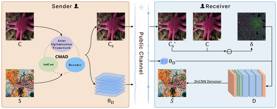
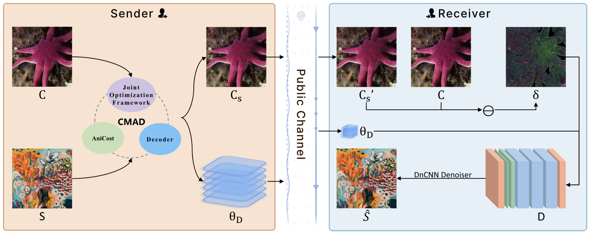
Let the cover image be and the secret image be , where and are the heights and widths of the cover and secret images, respectively. The receiver aims to recover from the stego image a secret image that is perceptually consistent with S. Before communication, the sender and receiver must pre-share the cover image C, the preprocessing operations, and the structural definition of the decoding network D. The sender transmits only the stego image and the decoding-network weights over the public channel. The receiver applies the agreed preprocessing to the cover image C, reads the received and normalizes it to , then computes , and inputs together with to the decoding network D to recover the secret image . The end-to-end procedure is shown in Figure 1.
Figure 1.
End-to-end system workflow. The sender inputs the cover image C and secret image S to the proposed CMAD method, which outputs the stego image and fine-tuned decoding-network weights . Both are transmitted to the receiver through a public channel. Using the pre-shared cover C, the receiver extracts the perturbation from and inputs together with to the decoding network D to recover the secret image .
Under this protocol, the adversary is assumed to have full access to the public channel and may intercept both the stego image and the decoder weights . The original cover image C is the only secret information that does not enter the public channel and is the system’s core security dependency. The receiver must possess the original cover image C to recover the secret image . The security evaluation in this paper is restricted to image-level steganographic detectability, namely, the ability of a steganalyzer to distinguish from ordinary images. The additional weight file in the transmitted data is not included in the security evaluation, and protocol-level covertness is left for future work.
To accommodate different transmission settings, we further design a robust variant, CMAD-R. Standard CMAD targets a lossless channel and prioritizes recovery quality and imperceptibility. CMAD-R introduces differentiable channel-attack simulation during joint optimization so that recovery fidelity can be retained under lossy conditions such as JPEG compression, Gaussian noise, and contrast adjustment. The internal structure of CMAD, corresponding to the expanded CMAD block in Figure 1, is detailed in Section 3.2. The notation used throughout this paper is summarized in Table 1.
Table 1.
Notation used in this paper.
3.2. Joint Perturbation-Embedding Optimization Framework
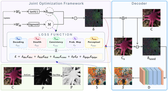
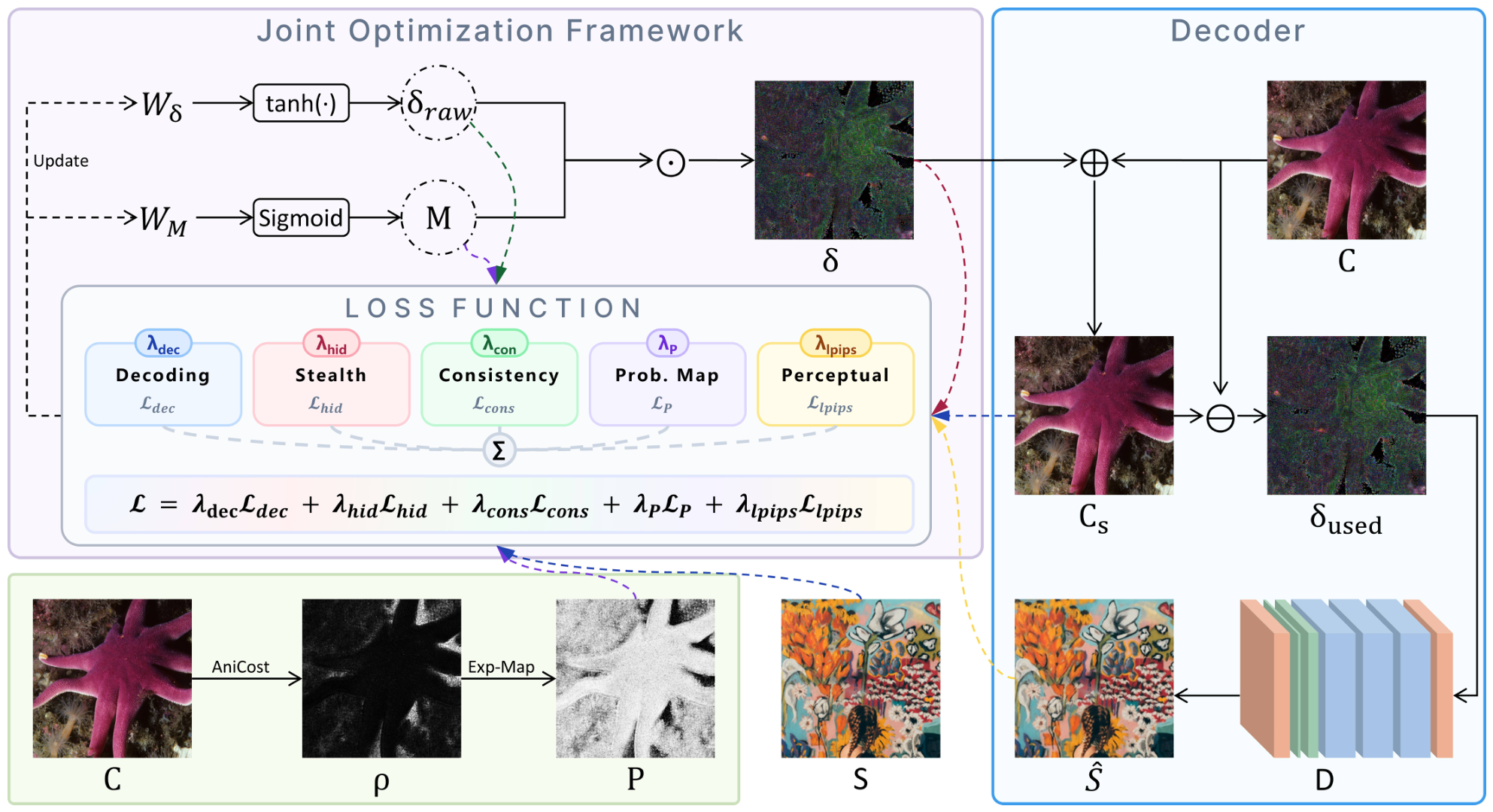
CMAD unifies embedding-location and modification-magnitude optimization within an end-to-end differentiable framework, thereby addressing their separation in existing methods. Its internal structure is shown in Figure 2. The framework parameterizes the optimization variables and to produce a physically feasible raw perturbation and mask M, which are fused into the final perturbation . The cost-guidance module applies the proposed AniCost algorithm to the cover image and computes a prior probability map P that guides the mask toward complex-texture regions. The decoder module adds the perturbation to the cover to synthesize , separates from using the cover, and recovers the secret image with D. The loss terms are aggregated and their gradients jointly drive updates to and , enabling the mask and perturbation to adapt cooperatively. Section 3.2.1, Section 3.2.2, Section 3.2.3, Section 3.2.4 and Section 3.2.5 present each module in detail.
Figure 2.
Internal structure and optimization workflow of CMAD.
3.2.1. Image Preprocessing
Before joint optimization begins, the cover and secret images undergo the same preprocessing pipeline, differing only in the target spatial size. During preprocessing, a given RGB image is read as an integer pixel array with values in [0,255], and all pixel values are divided by 255 to normalize to the floating-point range [0,1]. The scaling stage uses bilinear interpolation and reflective boundary padding and applies Gaussian low-pass filtering for anti-aliasing when the image size is reduced. After scaling, no quantization or integer rounding is performed. The processed cover image and secret image have pixel values stored as 32-bit floating-point numbers. This pipeline contains no random operations; under the same software environment and parameter settings, repeated execution on the same image yields identical results. Therefore, as long as both parties use the same preprocessing implementation, they are guaranteed to obtain the same cover image C.
3.2.2. Parameterization of the Perturbation and Mask
Given a cover image and an upper perturbation bound , we first compute a feasible interval for each pixel so that the modified pixel remains in and its absolute modification does not exceed :
where , , and index the row, column, and color channel, respectively. and are the minimum and maximum permissible perturbations at channel c of location .
A learnable variable is compressed to by a hyperbolic tangent and linearly mapped to , yielding a boundary-constrained raw perturbation :
The mask is a single-channel spatial weight map obtained by applying an elementwise sigmoid to the learnable variable :
The single-channel mask is expanded along the channel dimension into , with all channels sharing the same spatial weights:
The final perturbation is obtained by channel-wise weighting of the raw perturbation with the mask:
When , the perturbation is retained almost completely; when , it is suppressed and the pixel remains nearly unmodified. Joint optimization of and enables the mask and perturbation to converge cooperatively under the same gradient feedback, adaptively allocating both embedding locations and modification magnitudes.
To simulate the 8-bit quantization that occurs when a digital image is stored, a straight-through estimator is used to quantize the stego image into discrete pixel values during optimization. The stego image is first scaled from to , clipped and rounded, and then scaled back to :
Here, , and denotes rounding to the nearest integer. The forward pass follows Equation (6), whereas the gradient passes directly through the quantizer during backpropagation, i.e., . The perturbation actually used by the decoding network is
This design makes the optimization process more consistent with the physical properties of images after 8-bit storage and avoids an overoptimistic recovery estimate caused by a high-precision floating-point assumption. It should be noted that the cover image is not requantized to the 8-bit grid after resizing, and its pixels therefore remain continuous floating-point values. Consequently, even when the perturbation is zero, quantization may introduce into a small residual of at most . This residual is extremely small, and the decoding network can compensate for it adaptively during joint optimization; its effect on recovery quality is therefore negligible.
3.2.3. Cost-Map Guidance Mechanism
To guide the embedding perturbation toward complex-texture regions, we propose AniCost (Anisotropic Cost). Starting from the cover C, AniCost quantifies the sensitivity of each pixel to statistical detection through directional wavelet decomposition and anisotropy analysis. It outputs an embedding-cost map , in which a lower value denotes a location more suitable for embedding. An exponential mapping then converts into a prior embedding-probability map that serves as a spatial constraint in the loss function.
AniCost uses the Daubechies-8 (Db8) orthogonal wavelet. Its low-pass decomposition filter and high-pass decomposition filter form an orthogonal quadrature-mirror pair whose coefficients follow the canonical Db8 construction. Their outer products yield three two-dimensional directional filters:
Here, . is low-pass horizontally and high-pass vertically, making it sensitive to horizontal edges; behaves conversely and is sensitive to vertical edges; and is high-pass in both directions and responds to diagonal textures. Together, the three filters cover the principal texture orientations.
For channel c of the cover, denoted , symmetric reflection padding of pixels is first applied on all sides, producing . This suppresses artificial high-frequency components near boundaries caused by incomplete convolutional neighborhoods. is then convolved linearly in two dimensions with , , and . Because the Db8 filters have even length (16), each convolution output is shifted by half a pixel relative to the original grid. We therefore apply a positive circular shift of one pixel along both rows and columns, which is equivalent to relocating the origin from the filter center toward the higher-index side. Finally, the central region is cropped to obtain the directional energy-response maps .
At pixel , define the total directional energy and maximum directional energy as
where ensures numerical stability. describes the overall local texture strength, while measures directional concentration; values closer to one indicate stronger anisotropy. The single-channel pixel cost is
prevents division by zero when , while prevents reciprocal overflow if the entire denominator is zero. The expression has three progressively stronger effects. In a smooth region, is extremely small and the cost approaches a large saturation value, strongly suppressing embedding. As texture strength increases, the cost decreases. At equal texture strength, a larger directional concentration produces a larger term and a still lower cost because strongly directional textures, such as edges, mask perturbations more effectively than random textures and are less readily detected by steganalysis.
The denominator consists of , which increases monotonically with total texture strength, and an anisotropy ratio , which increases monotonically with directional concentration and is amplified by a factor of two. Consequently, the denominator increases with both and , whereas decreases monotonically. As , the denominator approaches and the cost approaches , strongly suppressing embedding in smooth regions. Increasing texture strength or anisotropy enlarges the denominator and lowers the cost. This monotonicity ensures high costs in smooth regions, lower costs in textured regions, and the lowest costs in strongly directional textured regions.
The costs of the three channels are summed pixelwise:
The median m is computed over pixels below the truncation limit . Median normalization is then applied as , followed by clipping at , which is the conventional extreme cost assigned to pixels regarded as completely unsuitable for embedding. Finally, an exponential mapping yields the prior embedding-probability map
P is subsequently linearly scaled to by dividing it by its maximum so that . Low-cost textured regions have P values close to one and are a priori suitable for embedding, whereas smooth regions have values close to zero. As the spatial weighting in the probability-map loss in Equation (16), P imposes an asymmetric constraint: in a high-P region, and the mask can expand freely; in a low-P region, and mask activation is strongly suppressed. The embedding region is thereby driven adaptively toward complex textures.
3.2.4. Loss Function
The joint objective is a weighted sum of five scalar losses, each averaged over its spatial dimensions. Let denote the single-channel soft mask and let be its three-channel broadcast.
The decoding loss measures pixelwise mean-squared error between the recovered secret image and the ground-truth secret image :
where is the Frobenius norm.
The concealment loss constrains the energy of the final perturbation and promotes imperceptibility:
The consistency loss forces the raw perturbation toward zero wherever the mask is closed, ensuring that modifications occur only where the mask permits them:
where is the sum of the absolute values of all elements and denotes elementwise absolute value.
The probability-map guidance loss uses the AniCost prior to impose a spatially selective constraint on M. A bidirectional guidance loss both suppresses activation in low-probability regions and encourages activation in high-probability regions:
The first term is suppressive. When P is close to one in a textured region, its weight is almost zero and the mask is barely penalized; when P is close to zero in a smooth region, the weight approaches one and the mask is strongly suppressed. The second term is activating: when P is close to one but M has not opened sufficiently, the large value of incurs a penalty that expands the mask over high-probability regions. Thus, the mask avoids ineffective modifications in smooth regions while remaining able to activate textured regions as required by the decoding loss, improving the trade-off between imperceptibility and secret-recovery accuracy.
The perceptual loss measures differences in a deep feature space to improve the subjective visual quality of the recovered image:
where LPIPS is computed with an AlexNet backbone.
The total objective is
The weights and are adjusted dynamically according to the current losses, as described in Section 3.2.5.
3.2.5. Coordinated Dynamic Weight Adjustment
To strengthen cooperative learning between the mask and perturbation, CMAD adaptively adjusts the decoding-loss weight and concealment-loss weight during optimization. Early in optimization, the perturbation is not fully formed and is high. must therefore increase progressively to prioritize secret recovery, encourage the mask to open in textured regions, and concentrate perturbation energy in recoverable locations. As optimization proceeds and perturbation energy decreases, increases concurrently, strengthening the imperceptibility constraint and suppressing perturbation magnitudes in flat regions. This coordinated adjustment allows the mask and perturbation to constrain and adapt to one another rather than being optimized independently. Specifically, grows according to the current decoding loss:
and grows according to the current perturbation energy:
The operation clips both weights to an upper bound of 50, ensuring numerical stability. To prevent instability caused by imbalanced gradient magnitudes among jointly optimized variables, a global gradient-norm clip of 1.0 is also applied to the perturbation variable, mask variable, and decoder parameters before every update. This keeps the perturbation mapping numerically stable and preserves coordinated convergence between spatial mask selection and perturbation-magnitude adjustment.
3.3. Decoding-Network Design and Fine-Tuning
After the joint-optimization framework determines the embedding region and perturbation magnitude, the decoding network must accurately recover the secret image from the perturbation. CMAD incorporates channel attention so that the network can adaptively focus on important feature channels. It also permits small updates to the decoding-network parameters during joint optimization, enabling dynamic adaptation to the current cover–secret pair. To further suppress high-frequency noise in the recovered image and improve its visual quality at the receiver, a pretrained DnCNN [21] is used for post-processing.
3.3.1. Network Architecture
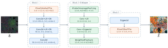
The input to D is the perturbation separated from the stego image, and the output is . As shown in Figure 3, PixelUnshuffle first reduces the spatial resolution and increases the number of channels to , where :
then passes through three convolutional layers. The first uses a kernel with stride 1 and produces 96 channels, followed by LeakyReLU and instance normalization. The strides and of the second and third layers depend on the ratio of cover to secret image size: for a ratio of two, for a ratio of four, and for equal sizes. Both kernels are . The first two layers maintain 96 output channels, while the third produces channels and has no activation function. Its output is passed directly to the channel-attention module, which adaptively emphasizes channels that are more important to recovery.
Figure 3.
Architecture of the decoding network D.
The channel-attention layer (CALayer) [22] globally average-pools an input feature map, generates channel weights through two convolutions, applies a sigmoid, and multiplies the weights channelwise with the original feature map:
Finally, the feature map passes through a sigmoid and PixelShuffle [23]. PixelShuffle reduces the channel count to three and restores the target spatial resolution , producing .
3.3.2. Weight Initialization and Fine-Tuning
The weights of D are randomly initialized by default. To accelerate convergence and improve recovery quality, joint optimization may first be performed over multiple cover–secret pairs. The resulting decoder weights can then be loaded as pretrained weights to initialize subsequent per-image-pair fine-tuning.
During joint optimization, Adam jointly updates the perturbation variable , soft-mask variable , and decoder parameters . The variables are divided into two parameter groups. The first contains and and uses the global learning rate; the second contains and uses half the global learning rate. Adam adaptively adjusts the step size of every variable from its gradient history.
The learning rate is scheduled with ReduceLROnPlateau. The mode is set to minimization, the decay factor is 0.8, the patience is 100, and the minimum learning rate is . After every optimizer update, the scheduler adjusts the learning rate according to changes in . This strategy retains the decoder’s existing feature-extraction ability while adapting it precisely to the current image pair.
3.3.3. Quantization Strategy
To generate a stego image, the soft mask modulates the continuous perturbation, which is then added to the cover. The resulting continuous stego image is mapped to the 8-bit integer domain: it is multiplied by 255, clipped to , quantized, and divided by 255 to recover a floating-point representation. The actual perturbation is the difference between the quantized stego image and the original cover and is input to the decoding network. Notably, the concealment loss is computed from the continuous perturbation, whereas the decoding loss is computed from the quantized, physically realized perturbation. Optimization therefore accounts for both a continuous-domain constraint and the actual written image.
Because quantization is nondifferentiable, a straight-through estimator (STE) approximates the rounding operation. The forward pass performs standard rounding, while the backward pass approximates the gradient with the identity map, i.e., the quantizer gradient is treated as one. Gradients can therefore traverse the nondifferentiable layer and enable end-to-end optimization. This mechanism allows effective updates to the perturbation and mask while accounting for actual 8-bit quantization.
4. Experiments
4.1. Experimental Setup
4.1.1. Datasets
Three public image datasets are used: COCO, CelebA, and DIV2K. In every experiment, the cover and secret images are resized to and , respectively. The raw secret-image source rate is 6 bpp, defined as the original size of the secret image, bits, divided by the number of cover-image pixels, .
4.1.2. Evaluation Metrics
The methods are evaluated from the following perspectives.
Visual quality. Let X and Y denote the original and evaluated images, respectively, and N the total number of pixels. Before computing the metrics, both images are rescaled from to the 8-bit intensity domain , so the pixel dynamic range is taken as , and the constants in PSNR, MAE, and SSIM are computed on this scale. The following four metrics are used:
- Peak signal-to-noise ratio (PSNR), which measures pixelwise mean-squared error,A higher value indicates less distortion.
- Structural similarity index measure (SSIM), which jointly evaluates luminance, contrast, and structural consistency,where and are the mean and standard deviation, , and . SSIM lies in , and a value closer to one indicates greater structural similarity.
- Learned perceptual image patch similarity (LPIPS) [24], computed with a linearly calibrated AlexNet backbone in a deep feature space. A lower value indicates greater perceptual similarity.
- Mean absolute error (MAE),where a lower value indicates more accurate reconstruction.
Resistance to steganalysis. Four steganalysis tools evaluate the detectability of the stego images: (a) StegExpose [25], a conventional statistical steganalysis tool; (b) YeNet [26], a deep-learning-based steganalysis network; (c) SRNet [27], an end-to-end model based on a deep residual network; and (d) SiaStegNet [28], a steganalyzer based on a Siamese convolutional neural network.
4.1.3. Hyperparameters
The core hyperparameters of CMAD are set as follows. The total number of optimization iterations is 2000, the initial learning rate is , and a ReduceLROnPlateau scheduler is used for dynamic adjustment. The upper bound on the perturbation magnitude is . The weights of the total-loss components are , , , , and . AniCost converts the cost map using the exponential mapping with a scaling factor of . The decoder is randomly initialized, and its fine-tuning learning rate is half the global learning rate. All experiments are conducted on a single NVIDIA RTX 5060 GPU. For the experiments in Section 4.2, Section 4.4, and Section 4.5, each group is run independently three times with random seeds 42, 23, and 54, and the statistical results are recorded; the observations for all cover–secret image pairs from the three runs are pooled for descriptive statistics, i.e., the mean and standard deviation are computed over all image-pair observations across the three runs.
4.2. Visual-Quality Analysis
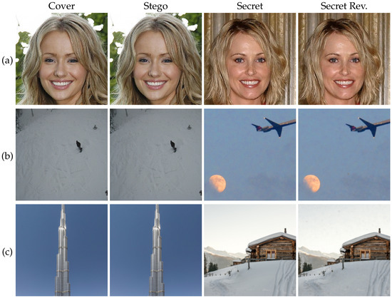
To evaluate the performance of CMAD, we compare it with two recent FNNS-based methods, Cs-FNNS [13] and RFNNS [14]. All three methods were rerun under a unified experimental protocol using the same dataset splits, image-pairing rule, input resolutions, quantization procedure, payload setting, evaluation metrics, and DnCNN post-processing. For CelebA and COCO-val2017, the first 2000 images in the predefined dataset order were selected. The first 1000 images were used as covers and the remaining 1000 as secrets, forming 1000 cover–secret pairs according to their corresponding indices. DIV2K contains 900 images; the first 450 were used as covers and the remaining 450 as secrets, forming 450 image pairs. The recovered secret images produced by all three methods were processed using the same DnCNN model. The quantitative results are reported in Table 2, and Figure 4 presents representative CMAD results on the different datasets.
Table 2.
Image-quality comparison of CMAD and state-of-the-art methods on different datasets (mean ± standard deviation). ↑ indicates larger is better, ↓ indicates smaller is better.
Figure 4.
Representative results generated by the proposed method: (a) CelebA; (b) COCO; and (c) DIV2K. The columns show the cover, stego image, secret image, and recovered secret, respectively.
From Table 2, under the same image size and source-rate settings, CMAD outperforms Cs-FNNS and RFNNS in image quality, but at the cost of transmitting an additional message-specific decoder weight file of about 411 KB, which the comparison methods do not require. Specifically, the stego-image PSNR improves over Cs-FNNS by 13.06 dB, 17.83 dB, and 12.43 dB on COCO, CelebA, and DIV2K, respectively, and over RFNNS by 12.10 dB, 15.89 dB, and 13.13 dB; SSIM, LPIPS, and MAE follow the same trend. The recovered-secret PSNR improves over Cs-FNNS by 4.01 dB, 5.12 dB, and 3.90 dB, and over RFNNS by 5.93 dB, 7.19 dB, and 5.82 dB on the three datasets, with SSIM, LPIPS, and MAE of the recovered images also superior. However, the standard deviations of CMAD metrics are generally larger than those of the comparison methods, which are all below 1 dB, indicating that the influence of different cover images on optimization results is more pronounced for CMAD.
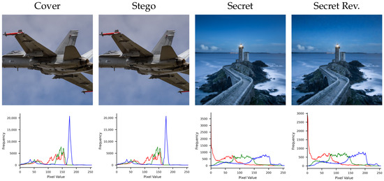
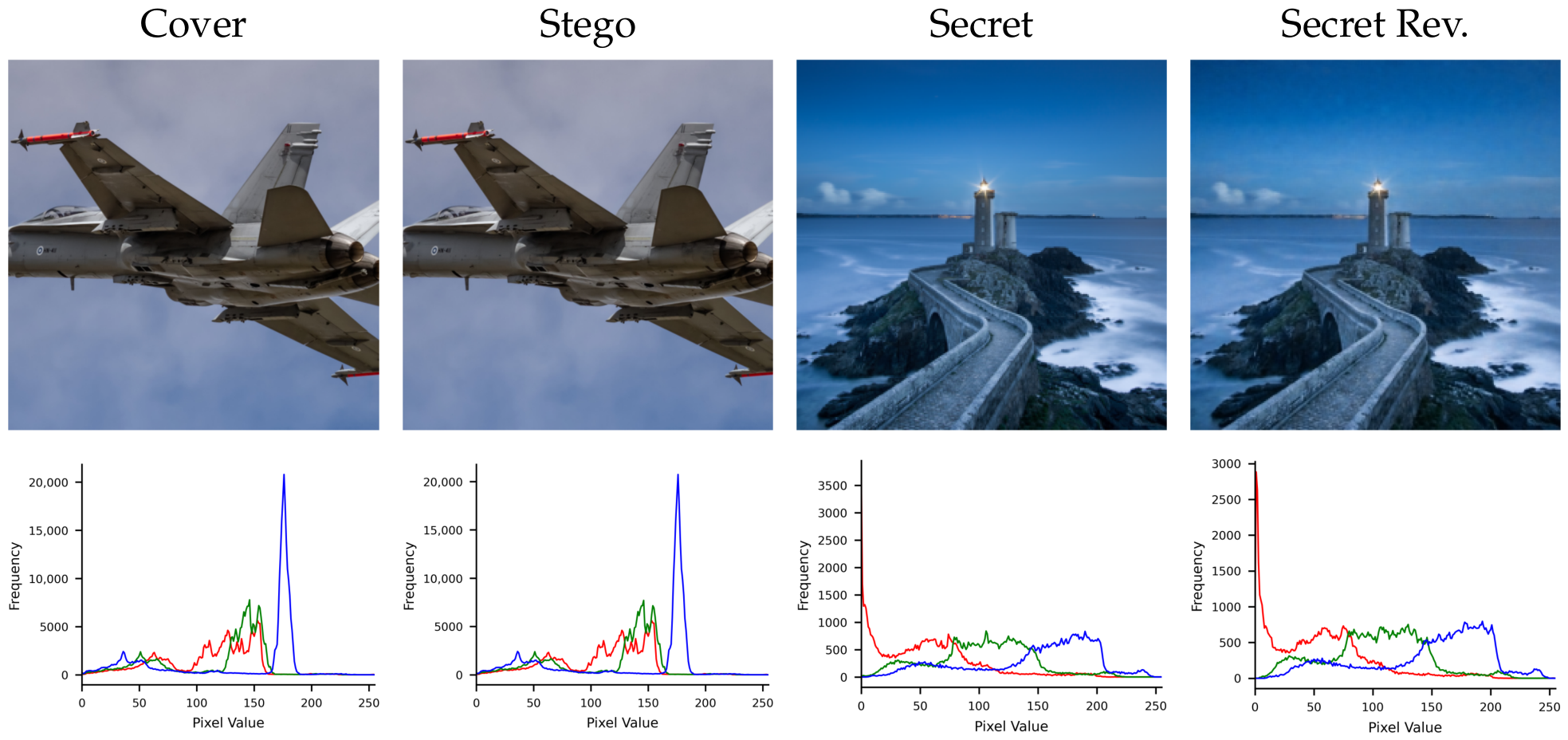
Figure 5 compares the RGB-channel histograms of the cover and stego images. Their distributions almost completely overlap, indicating that the CMAD perturbation causes no appreciable shift in the first-order pixel distribution.
Figure 5.
Comparison of RGB-channel histograms for representative experimental images. The first row shows the original images, and the second row shows the corresponding RGB-channel histograms (red, green, and blue curves represent the respective color channels).
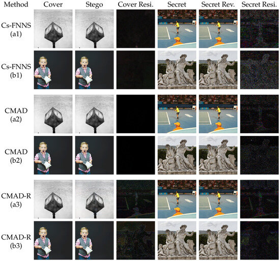
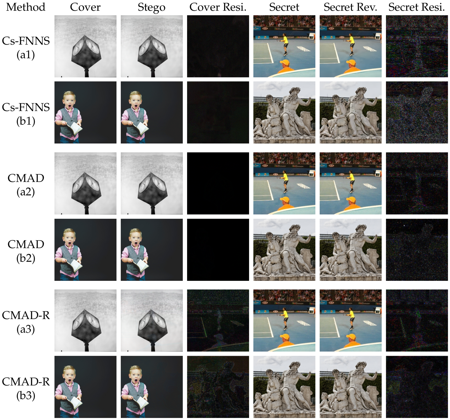
Figure 6 visually compares CMAD and Cs-FNNS [13] on COCO and DIV2K. It shows the residual between each stego and cover image, magnified tenfold, and the residual between each recovered and original secret image, also magnified tenfold. CMAD introduces an extremely weak stego residual that remains almost entirely black even after magnification, while the Cs-FNNS residual is similarly weak. The recovered-secret residual of CMAD is clearly smaller than that of Cs-FNNS.
Figure 6.
Visual comparison among CMAD, Cs-FNNS, and CMAD-R using samples from (a1–a3) COCO and (b1–b3) DIV2K. Residuals are magnified by a factor of ten.
4.3. Resistance to Steganalysis
Consistent with the threat model defined in Section 3.1, the evaluation in this subsection considers only the stego image and does not consider the fine-tuned decoder weights transmitted as part of the complete CMAD protocol. Accordingly, the reported detection accuracy quantifies image-level steganographic detectability rather than the detectability of the complete protocol.
For the deep-learning detectors, we consider two training assumptions: a universal detector and a CMAD-specific detector. The training and validation data are drawn from the COCO and CelebA datasets. We first exclude the first 2000 images from each dataset because these images were already used for the visual-quality evaluation in Section 4.2. From the remaining images, 1500 cover images are randomly selected from each dataset, yielding 3000 covers in total. Both detector settings use these 3000 covers to generate stego images. For the universal detector, 1000 stego images are generated by Cs-FNNS, 1000 by StegGAN, 500 by S-UNIWARD, and 500 by WOW. For the CMAD-specific detector, CMAD generates one corresponding stego image for each cover. The resulting 3000 cover–stego pairs are then randomly divided in an 8:2 ratio into 2400 training pairs and 600 validation pairs. The independent test set consists of the 2450 image pairs already generated in Section 4.2, including 1000 COCO pairs, 1000 CelebA pairs, and 450 DIV2K pairs. All detection accuracies reported in Table 3 are obtained on this independent test set.
Table 3.
Steganalysis detection accuracy for CMAD on different datasets (mean ± standard deviation). Accuracy closer to the random-guessing level of 50% indicates lower detectability.
All steganalysis networks are trained using the Adam optimizer with a weight decay of , an initial learning rate of , and a batch size of 4. The learning rate is halved every 30 epochs, and each network is trained for 100 epochs. For each detector, three instances are trained using random seeds 42, 23, and 54, respectively. During training, the checkpoint with the best validation-set performance is retained as the final model for that seed, and this model is then evaluated once on the independent test set to obtain the detection accuracy for that seed. Finally, the detection accuracies from the three seeds are averaged to produce the reported result for that detector on the corresponding dataset, along with the standard deviation. The results are shown in Table 3.
CMAD’s detectability varies across datasets. In the universal setting, CelebA produces accuracies closest to random guessing, whereas COCO and DIV2K are more detectable. On DIV2K, YeNet reaches 63.91%, while SiaStegNet and SRNet reach 60.38% and 58.97%, respectively. In the specific setting, accuracy rises substantially on every dataset; SRNet reaches 74.15% on DIV2K, and YeNet reaches 75.36% on CelebA. These results describe detection difficulty only under the present system configuration and threat model. CMAD shows limited resistance to detectors not trained specifically on CMAD, but further improvement is needed on COCO and DIV2K, and its overall resistance to a detector trained specifically for CMAD remains limited.
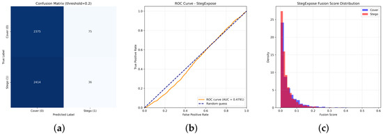
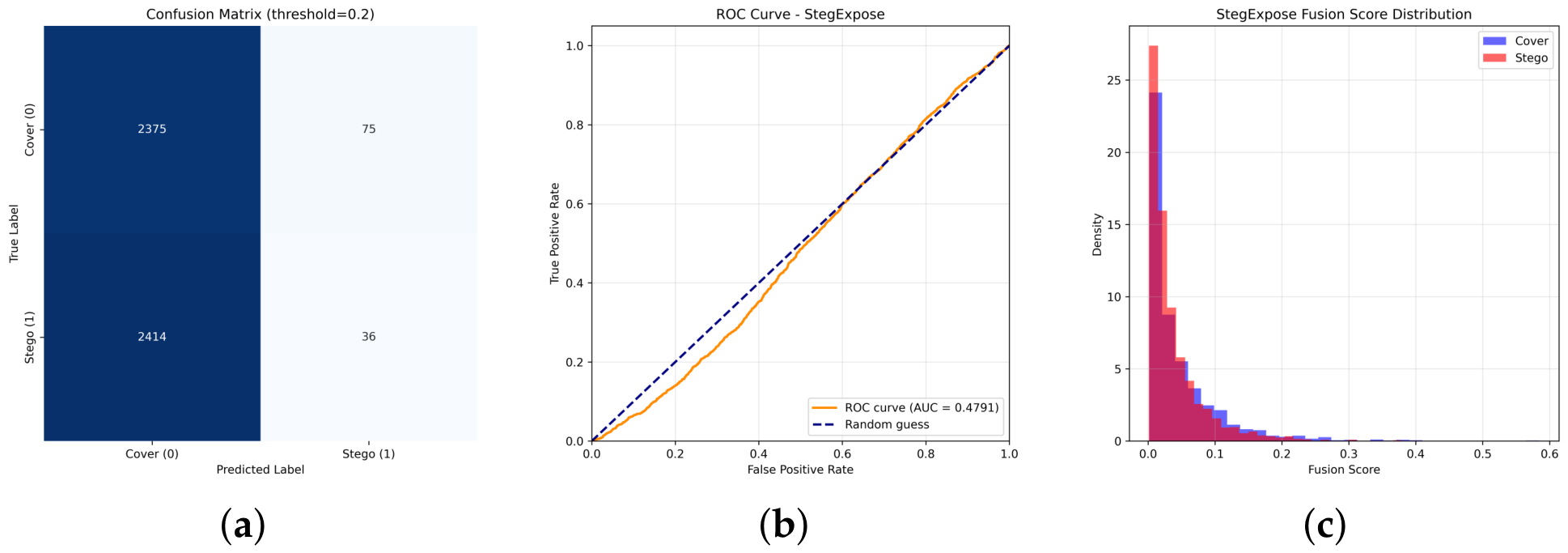
Figure 7 shows the results of StegExpose on CMAD stego images. The cover and stego score distributions overlap substantially, so no threshold effectively separates them. The receiver-operating-characteristic (ROC) curve closely follows the diagonal random-guessing reference, with an area under the curve (AUC) of only 0.4791. StegExpose’s conventional statistical features are therefore almost entirely unable to identify CMAD stego images.
Figure 7.
StegExpose detection results for CMAD-generated stego images. (a) Confusion matrix. At the default threshold of 0.2, the detection rate is only 1.47%. (b) ROC curve constructed by varying the threshold over continuous scores; the dashed line is random guessing. (c) Score-distribution histogram. The cover and stego fusion-score distributions and their density curves substantially overlap.
4.4. Robustness Evaluation
CMAD achieves high imperceptibility and recovery quality under lossless transmission, but its recovery performance deteriorates substantially under channel attacks. To improve robustness, we construct CMAD-R. At each optimization iteration, an attack is triggered with a probability of 0.2. When an attack is triggered, one of three training attacks—JPEG compression, Gaussian noise, or contrast adjustment—is selected uniformly at random and applied to the current stego image . The decoder then reconstructs the secret image from the attacked perturbation . For each attack, the attack-induced distortion residual is detached from the computational graph and added to the original perturbation, allowing gradients to propagate only through the path. An attack-recovery loss, , with a weight of 0.5 is added to the original objective. Attack simulation is used only during optimization. At test time, each attack is applied directly to an unattacked stego image.
The robustness experiments are conducted on DIV2K, using the first 450 images as covers and the remaining 450 as secrets. The cover and secret images are resized to and , respectively, and all other hyperparameters are identical to those of standard CMAD. Six attacks are evaluated at test time: JPEG compression with a quality factor of QF = 80; additive white Gaussian noise with a standard deviation of ; contrast adjustment with a factor of , where leaves the image unchanged and reduces the contrast according to , with denoting the mean of ; scaling with a factor of , implemented by downsampling the image to 95% of its original size and restoring it using bilinear interpolation; Gaussian blur with a standard deviation of ; and random cropping with a retention ratio of , followed by bilinear resizing to the original spatial resolution. During training, only JPEG compression, Gaussian noise, and contrast adjustment are used, with weaker settings of QF = 90, , and , respectively. Scaling, Gaussian blur, and cropping are not included during optimization and are used to evaluate generalization to unseen attack types. Each experiment is repeated using multiple random seeds, and the averaged results are reported.
As shown in Table 4, standard CMAD achieves a stego-image PSNR of 55.09 dB in the absence of attacks, but its recovered-secret PSNR decreases substantially under channel attacks, demonstrating its dependence on an accurate residual. CMAD-R reduces the unattacked stego-image PSNR to 40.38 dB but improves the recovered-secret PSNR by 6.02–15.58 dB across the six evaluated attacks. Compared with RFNNS, CMAD-R achieves comparable recovery quality under JPEG compression, scaling, and Gaussian blur, but remains weaker under Gaussian noise, contrast adjustment, and cropping. These results indicate that attack-aware optimization substantially improves robustness, although further improvement is required for stronger noise, contrast distortion, and geometric content loss.
Table 4.
Quality of stego and recovered-secret images under different attacks. ↑ indicates larger is better, ↓ indicates smaller is better.
4.5. Ablation Studies
4.5.1. Effectiveness of Decoder Fine-Tuning and Channel Attention
Three variants evaluate the contribution of decoder fine-tuning and channel attention: a static decoder (Static Dec.), no channel attention (No CA), and both mechanisms disabled (Static Dec. & No CA). Table 5 reports the results.
Table 5.
Image-quality comparison among decoder variants. ↑ indicates larger is better, ↓ indicates smaller is better.
Disabling decoder fine-tuning reduces stego-image PSNR from 55.46 to 35.82 dB and recovered-secret PSNR from 37.04 to 27.45 dB; the corresponding SSIM values fall to 0.7736 and 0.8074. A static decoder therefore cannot adapt to the current image pair and forces the optimizer to increase the perturbation to compensate for insufficient decoding capacity. Removing channel attention reduces stego-image PSNR further to 30.75 dB, while recovered-secret PSNR is 30.12 dB, confirming the importance of channel attention for feature selection. When both mechanisms are disabled, recovered-secret PSNR falls to 12.20 dB and SSIM to 0.2287; decoding almost entirely fails. The degradation is greater than when either mechanism is removed alone, showing that decoder adaptation and channel attention are mutually dependent.
4.5.2. Effectiveness of AniCost Guidance
AniCost is evaluated on the first 200 DIV2K images, with the first 100 serving as covers and the remaining 100 as secrets. Every experiment is repeated with multiple random seeds, and the mean and standard deviation are reported. The comparison priors are No Prior (), Uniform Prior (), Random Prior (), Inverse AniCost (), the WOW cost map, the S-UNIWARD cost map, and AniCost. Table 6 reports stego-image and recovered-secret quality for each prior.
Table 6.
Image-quality comparison under different cost-guidance priors. ↑ indicates larger is better, ↓ indicates smaller is better.
No Prior and Uniform Prior produce similar results. Without content-adaptive cost guidance, the optimizer tends to reduce the decoding loss by increasing the perturbation globally, sharply lowering stego-image PSNR and seriously compromising imperceptibility. Although recovered-secret PSNR is relatively high, it is obtained at the cost of concealment. AniCost concentrates perturbation energy in textured regions, achieving a stego-image PSNR of 55.46 dB while retaining a recovered-secret PSNR of 37.04 dB and thus providing the best trade-off between imperceptibility and recovery. Compared with AniCost, WOW and S-UNIWARD have stego-image PSNR values that are 3.15 and 2.27 dB lower and recovered-secret PSNR values that are 1.75 and 1.34 dB lower, respectively. AniCost provides a more favorable empirical trade-off under the evaluated configuration. Random Prior lacks content adaptivity and reaches only 35.45 dB for recovered-secret PSNR. Inverse AniCost directs perturbations toward flat regions and reduces recovered-secret PSNR further to 33.70 dB, confirming that the direction of the cost prior influences embedding locations.
4.5.3. Information-Carrier Validation and Security Analysis
Controlled experiments are conducted on 100 DIV2K pairs by reusing generated cover–stego pairs and their corresponding fine-tuned weights. The tested conditions include zero perturbation, random perturbation, swapped decoders, fixed inputs, averaged weights, randomly initialized decoders, cover estimation and mismatch, and training driven by fixed noise. DnCNN post-processing and 8-bit quantization are used throughout. The combination of the correct perturbation and correct fine-tuned weights serves as the baseline. Table 7 summarizes the configurations and recovery quality.
Table 7.
Configurations and recovery quality in the information-carrier validation experiment.
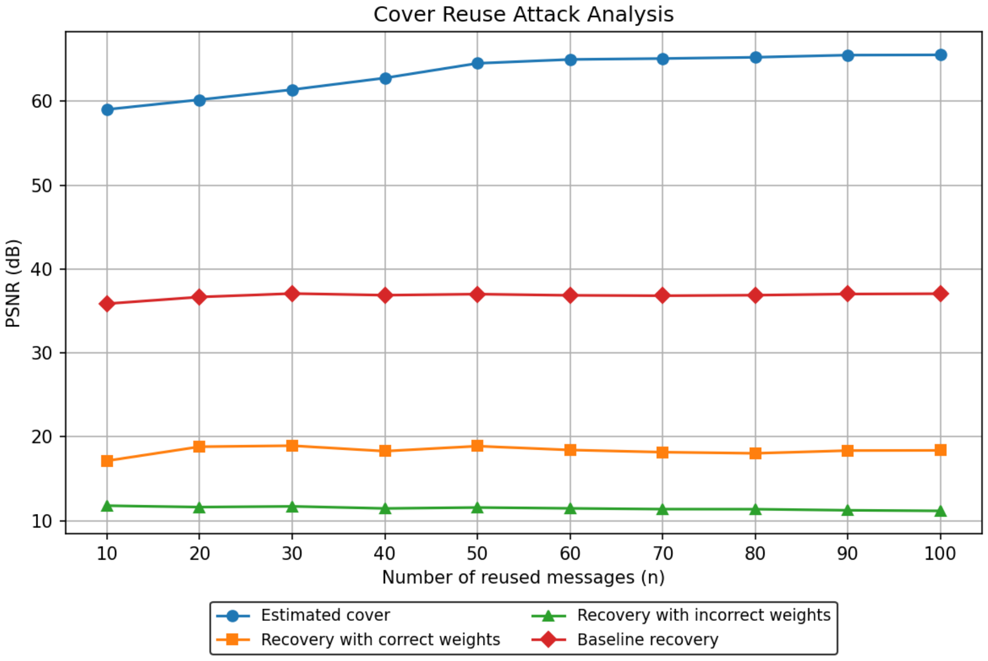
The experimental results show that the recovered-secret PSNR remains below 12 dB under zero perturbation, random perturbation, and all fixed-input conditions. Decoder swapping and weight averaging also yield recovered-secret PSNR values of only 17.69 and 20.28 dB, respectively, far below the baseline of 37.04 dB. These findings indicate that a valid perturbation and the matching weights are both indispensable for secret recovery. Cover-estimation and cover-mismatch attacks both reduce the recovered-secret PSNR to approximately 10.7 dB, further demonstrating that decoding is highly dependent on the exact cover. The cover-reuse experiment in Appendix E shows that even when an attacker averages multiple stego images to obtain an estimated cover with a PSNR as high as 65.5 dB, the recovered-secret PSNR remains only approximately 18 dB, indicating that a high-precision estimate cannot substitute for the exact cover. Once the exact cover is compromised, however, an attacker can directly extract the exact perturbation from the stego image and combine it with the intercepted fine-tuned weights to raise the recovered-secret PSNR to the baseline level of approximately 37 dB, thereby fully exposing the secret. Therefore, under the evaluated averaging attack, for the tested cover, effective recovery was not achieved with up to 100 reused messages. The protocol permits cover reuse, but its core security assumption is that the exact cover must remain strictly confidential.
In the control experiment with fixed-noise-driven fine-tuning, the decoder receives the same fixed random noise during training and testing, and the perturbation does not participate in decoding. The recovered-secret PSNR is 10.78 dB. Although the weights exhibit some memorization capability, they do not enable effective recovery. This result shows that successful recovery depends jointly on the image perturbation and the corresponding message-specific decoder weights.
4.5.4. Effect of the Dynamic Weight-Scheduling Strategy
Five schedules evaluate the adaptive dynamic strategy in Equations (19) and (20): (1) Adaptive, the proposed threshold-based multiplicative-growth strategy with upper-bound clipping; (2) Const-Small, which fixes the initial weights and ; (3) Const-Large, which fixes manually tuned values and ; (4) Stepwise, which applies and every 200 iterations with an upper bound of ; and (5) Reciprocal, which sets and at every iteration, where . Experiments use the first 200 DIV2K images, divided equally into covers and secrets, and are repeated with multiple random seeds. Table 8 reports the mean and standard deviation.
Table 8.
Image quality under different weight-scheduling strategies on DIV2K and COCO (mean ± standard deviation). ↑ indicates larger is better, ↓ indicates smaller is better.
The schedules exhibit a clear trade-off between stego imperceptibility and secret recovery. Adaptive gives the best overall stego-image quality. Its recovered-secret PSNR is 37.04 dB, less than 3 dB below Reciprocal, Stepwise, and Const-Large. Const-Small retains reasonable stego quality but produces the lowest recovered-secret PSNR because its small static weights provide insufficient decoding pressure. Const-Large and Stepwise improve recovery but reduce stego-image PSNR by more than 14 dB relative to Adaptive. Reciprocal achieves the highest recovered-secret PSNR, but its stego-image PSNR is only 36.71 dB; moreover, its stego and recovered-secret PSNR standard deviations are 2.95 and 5.26 dB, respectively. The inverse-loss weights therefore fluctuate strongly and destabilize optimization. Overall, Adaptive provides the best balance and demonstrates the importance of adaptive multiplicative growth to joint mask–perturbation optimization.
4.6. Communication Overhead and Computational Efficiency
The overhead of the complete CMAD protocol comprises pre-shared information and per-message transmission. Before communication, the sender and receiver pre-share the structural definition of D and the original cover C. The network description is approximately 1.86 KB, whereas the cover size depends on the image. For each message, the sender transmits and through the public channel. The stego-image size is approximately the same as that of the cover, and the weight file is 411 KB.
For every cover–secret pair, the sender performs 2000 joint-optimization iterations, whereas the receiver performs only decoding, which takes approximately 2 s. The sender requires approximately 27 s per pair for CMAD, 12 s for Cs-FNNS, and 24 s for RFNNS. CMAD is slower because joint mask–perturbation optimization and decoder fine-tuning require additional backpropagation. Peak memory use is approximately 1809.3 MB for CMAD, 1154.3 MB for Cs-FNNS, and 1906.1 MB for RFNNS. CMAD therefore lies between the two comparison methods and fits within the memory capacity of the experimental GPU. These measurements use one NVIDIA RTX 5060 GPU with 8 GB of memory, cover images, secret images, and raw secret-image source rate of 6 bpp.
5. Conclusions
This paper proposed CMAD, an adaptive steganographic method based on cost-guided joint mask–perturbation optimization. CMAD jointly optimizes the embedding mask and perturbation magnitude in an end-to-end differentiable framework and combines AniCost guidance with a channel-attention decoding network. On COCO, CelebA, and DIV2K, its stego images achieve PSNR values of 55–60 dB, and its recovered secret images achieve PSNR values of 35–40 dB. CMAD approaches random-guessing performance against conventional statistical steganalysis, but its resistance to deep-learning-based steganalyzers requires further improvement. CMAD-R retains some recovery capability under JPEG compression, contrast adjustment, and other attacks, providing a lossy-channel variant of CMAD. Ablation results identify AniCost guidance as essential to balancing imperceptibility and recovery quality. Information-carrier validation further shows that successful recovery depends jointly on the image perturbation and the corresponding message-specific decoder weights. The mask, cost guidance, and attention-based fine-tuning are all necessary within the joint-optimization framework.
When only the stego images are considered, CMAD approaches random-guessing performance under conventional statistical steganalysis, but its resistance to deep-learning-based steganalyzers still requires further improvement. In addition, the complete CMAD protocol also transmits fine-tuned decoder weights, which may reveal the use of CMAD. The security claims in this paper are therefore restricted to image-level steganographic detectability, while protocol-level covertness remains an open challenge for future work. The robustness of CMAD-R against attacks such as Gaussian noise also remains to be improved.
Author Contributions
Conceptualization, Q.L. and X.C.; Methodology, Q.L.; Software, X.C.; Validation, Q.L., X.C., H.W., Z.W. and M.L.; Formal Analysis, Q.L. and H.W.; Investigation, Q.L., Z.W. and M.L.; Resources, Q.L.; Data Curation, X.C., H.W. and M.L.; Writing—Original Draft Preparation, X.C.; Writing—Review and Editing, Q.L., X.C., H.W., Z.W. and M.L.; Visualization, Z.W.; Project Administration, Q.L.; Funding Acquisition, Q.L. All authors have read and agreed to the published version of the manuscript.
Funding
This work was supported by Key Research Project of Gansu University of Political Science and Law under Grant No.GZF2025XZD19.
Data Availability Statement
The data used in this study are publicly available datasets. COCO is available at https://cocodataset.org; CelebA is available at https://mmlab.ie.cuhk.edu.hk/projects/CelebA.html; DIV2K is available at https://data.vision.ee.ethz.ch/cvl/DIV2K/. All datasets were accessed on 13 December 2025.
Conflicts of Interest
The authors declare no conflicts of interest.
Appendix A. Communication Overhead and Capacity Analysis
Appendix A.1. Communication Overhead
The primary communication-overhead difference among CMAD, Cs-FNNS, and RFNNS lies in decoder-weight transmission. Their pre-sharing overheads are of comparable magnitude: the Cs-FNNS decoder architecture requires approximately 4.73 KB, the RFNNS architecture 6.05 KB, and the CMAD architecture 1.86 KB. These are one-time costs that are much smaller than the transmission required for each message. Cs-FNNS and RFNNS generate their covers from prompts and therefore require the sender and receiver to share a prompt in addition to the decoding network. CMAD can use any image as its cover. However, the cover must be treated as secret. The sender and receiver must pre-share the cover through a confidential channel. Merely downloading the same image from a public source is not secure, because an adversary could also access that source and reconstruct the cover.
Per-message transmission constitutes the main difference. Assuming that a RGB image occupies approximately 768 KB, Cs-FNNS and RFNNS initialize their decoder weights from a shared seed and do not transmit a weight file; each message therefore contains only an approximately 768 KB stego image. CMAD fine-tunes its decoder for each image pair and must transmit an additional 411 KB of weights, for a total of approximately 1179 KB per message. Under an equal total budget of 1179 KB, Cs-FNNS and RFNNS can allocate the full budget to the stego image, whereas CMAD allocates 411 KB to the weights and approximately 768 KB to the stego image. All three methods remain within the same order of magnitude, from several hundred kilobytes to approximately 1 MB per message. CMAD exchanges an additional 411 KB for the image-quality improvements reported in Table 2.
Appendix A.2. Estimated Information in Residual and Weight Increment
We separately estimate the effective information carried by the image residual and the transmitted fine-tuned weight increment. The original secret contains 192 KB ( bits). Nonzero elements of are discretized into 256 equal-width bins, yielding a total residual entropy of bits, or approximately 25 KB of effective information. Applying the same procedure to the weight increment yields bits, or approximately 40 KB.
Appendix A.3. Comparison with Cryptography
For a cover and a secret, the original secret occupies approximately 192 KB. CMAD transmits an approximately 768 KB stego image and 411 KB of decoder weights, for a total of approximately 1179 KB and a transmission ratio of about 6.1:1; approximately 6.1 transmitted bits are required per useful recovered bit. Cs-FNNS and RFNNS transmit only an approximately 768 KB stego image, producing a ratio of approximately 4:1. In bit efficiency alone, CMAD is therefore less efficient because it transmits decoder weights. In multi-message settings, the 1–6 KB decoder-architecture descriptions are one-time pre-sharing costs and can be amortized, as can a pre-shared cover if it is reused by a sender. CMAD’s 411 KB weight file, however, is specific to each message and cannot be amortized. Its overhead accumulates linearly over a long sequence of messages, which is an inherent cost of per-image decoder fine-tuning.
If bit efficiency is the only criterion, encrypting the secret with a standard cipher such as AES-256 produces ciphertext approximately equal in size to the plaintext and a transmission ratio of about 1:1, substantially better than all three steganographic methods. This comparison highlights the fundamental distinction between steganography and cryptography. Encryption protects message content but does not conceal the existence of communication. The ciphertext generated by direct encryption appears as a random bitstream; its detectability depends on the specific protocol and traffic context, and in some cases it may be identified as encrypted communication and raise suspicion. Steganography hides secret information in an apparently ordinary image and seeks to make the stego image visually and statistically indistinguishable from a normal image, concealing the act of communication itself. The two technologies therefore solve different problems and serve different use cases.
Appendix B. CMAD Performance Statistics and Robustness
Unless otherwise stated, the appendix experiments are conducted on the first 200 images of the DIV2K dataset, with the first 100 serving as covers and the remaining 100 as secrets. Cover and secret image sizes are set to and , respectively. Each experiment is repeated with random seeds 42, 23, and 54, and the mean and standard deviation are computed over all image-pair observations across the three runs.
Table A1.
Mean, standard deviation, and variance of CMAD quality metrics on different datasets. The dataset partitioning is the same as in 4.2. ↑ indicates larger is better, ↓ indicates smaller is better.
Table A2.
CMAD-R image quality under compound attacks. ↑ indicates larger is better, ↓ indicates smaller is better.
Table A3.
Paired comparisons between CMAD and the comparison methods on identical cover–secret image pairs. For each cover–secret image pair, the metric for each method (CMAD, Cs-FNNS, and RFNNS) is first averaged over the three random-seed runs to obtain a representative value for that image pair. Paired differences are then computed as CMAD minus the corresponding comparison method using these averaged values. SD denotes the standard deviation of the paired differences across independent image pairs. The 95% confidence intervals are computed using the t-distribution, and the reported p-values are obtained from two-sided paired-sample t-tests with the image pair as the statistical unit. Sample sizes: COCO n = 1000, CelebA n = 1000, DIV2K n = 450.
Table A4.
Mean, standard deviation, and variance of recovered-secret quality before and after DnCNN denoising. The dataset partitioning is the same as in 4.2. ↑ indicates larger is better, ↓ indicates smaller is better.
Appendix C. Embedding Distribution and Optimization Convergence
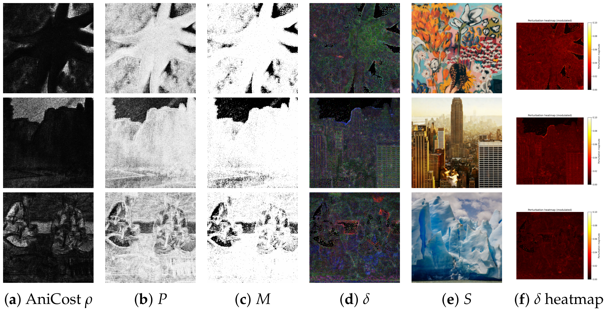
Table A5 shows that 84.24% of pixels are activated, while the mean mask value is only 0.0298 and mask entropy is only 0.115. Perturbation energy in textured regions is approximately 4.2 times that in smooth regions. Most pixels therefore receive only extremely small modifications, and the spatial distribution is biased toward complex textures. The final gradient norms are on the order of , indicating that optimization is close to convergence. Figure A1 shows the dynamic trajectories of and together with the gradient trajectories. Figure A2 shows the cost, probability, mask, and perturbation maps.
Table A5.
Embedding spatial-distribution and optimization-convergence metrics (mean ± SD) over 100 DIV2K cover–secret pairs. Smooth and textured regions are separated at the median AniCost . Gradient norms are the norms of the final-iteration gradients with respect to and .
Figure A1.
Dynamic trajectories of and and the corresponding gradient trajectories. Different colors represent different groups of images.
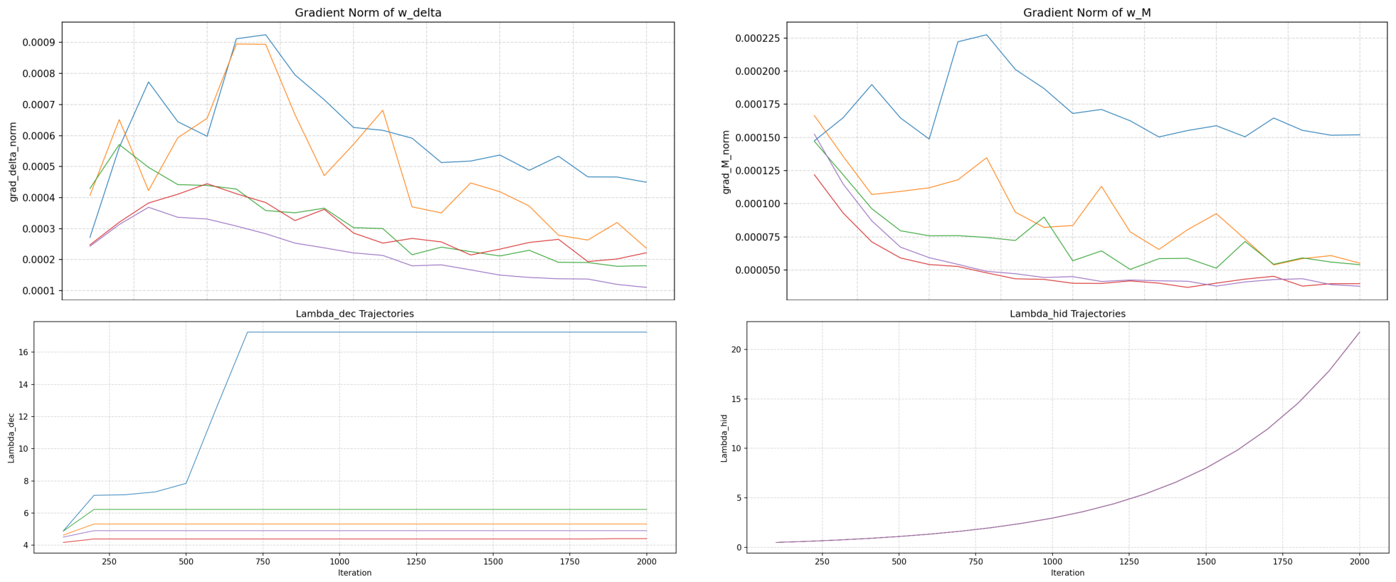
Figure A2.
Spatial maps produced during CMAD optimization.
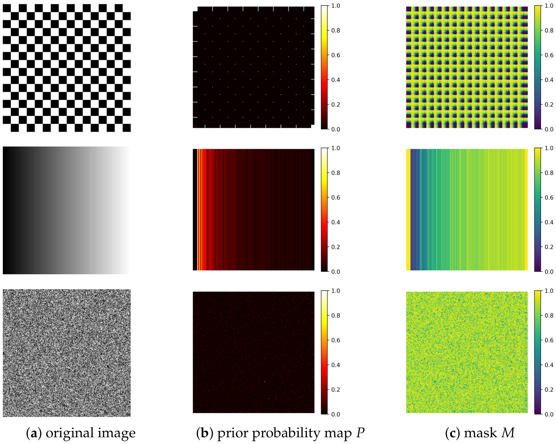
Appendix D. Controlled Synthetic Examples
Figure A3.
Controlled synthetic examples. Within each row, the images from left to right are the original image, prior probability map P, and mask M.
Appendix E. Cover Reuse
One DIV2K cover is fixed, and the attacker is assumed to intercept all stego images and their corresponding fine-tuned weights while not knowing the original cover. The attacker calculates the pixel-wise average of the first n stego images as the estimated cover, extracts the perturbations using this estimated cover, and recovers the secrets using either the correct fine-tuned weights or decoder weights obtained by weight averaging. Table A6 reports the results at representative values of n.
Table A6.
Results of the cover-reuse attack.
Figure A4 presents the complete trends. The horizontal axis denotes the number of reused messages n, and the vertical axis denotes PSNR (dB). The estimated-cover PSNR rises from approximately 60 dB to 65.5 dB as n increases and then tends to saturate. The recovery PSNR obtained using the estimated cover and the correct weights remains at 18–19 dB, whereas the baseline recovery PSNR obtained using the true cover remains stable at approximately 37 dB. Recovery with averaged weights yields a PSNR of approximately 11 dB, which is indistinguishable from random guessing. These results show that even if an attacker intercepts all stego images and weights, averaging alone cannot produce a cover sufficiently accurate for effective secret recovery, which remains far below the baseline.
Figure A4.
Trends in estimated-cover accuracy and secret-recovery quality as the number of reused messages increases in the cover-reuse attack.
Appendix F. Sensitivity to α and Wavelet Selection
The sweep fixes the wavelet to Db8, while the wavelet sweep fixes . Table A7 shows that increasing concentrates P more strongly in low-cost regions, reduces the activated-pixel ratio, and increases stego-image PSNR, but decreases recovered-secret PSNR. An overly strong prior therefore restricts the available modification locations and harms recovery. Table A8 shows that directional frequency resolution improves from Db1 to Db8, allowing the cost map to characterize textured edges more precisely. The activated-pixel ratio falls while both stego-image and recovered-secret PSNR increase, indicating that Db8 provides better texture discrimination and embedding guidance.
Table A7.
Sensitivity to the exponential-mapping factor .
Table A8.
Sensitivity to wavelet selection.
Appendix G. Deployability Analysis on Edge Processors
The deployment analysis in this work is based on experimental results obtained on a single NVIDIA RTX 5060 GPU with 8 GB of memory. On the sender side, CMAD requires 2000 joint optimization iterations per image pair, with an average runtime of approximately 27 s and a peak memory usage of about 1809 MB. This computational cost is suitable for high-performance personal computers equipped with discrete GPUs or edge servers, but remains impractical for real-time processing on low-power edge nodes. On the receiver side, only a single forward decoding pass is required, taking approximately 2 s, which is computationally lightweight and amenable to deployment on resource-constrained edge devices. With additional techniques such as network pruning and 8-bit quantization, the decoder can be further compressed and accelerated using edge NPUs.
To alleviate the sender-side computational bottleneck, adaptive early stopping can be introduced to reduce the number of optimization iterations, while mixed-precision training and partial parameter freezing can be employed to lower memory consumption and computational overhead. Overall, CMAD exhibits an asymmetric deployment profile: the sender is computationally intensive, whereas the receiver is lightweight and can be migrated to edge terminals. With the aforementioned strategies, the sender side has the potential to approach near-real-time operation on edge nodes with moderate computational capacity.
References
- Song, B.; Wei, P.; Wu, S.; Lin, Y.; Zhou, W. A survey on deep-learning-based image steganography. Expert Syst. Appl. 2024, 254, 124390. [Google Scholar] [CrossRef] [Scilit]
- Luo, W.; Wei, K.; Li, Q.; Ye, M.; Tan, S.; Tang, W.; Huang, J. A comprehensive survey of digital image steganography and steganalysis. APSIPA Trans. Signal Inf. Process. 2024, 13, 2024. [Google Scholar] [CrossRef] [Scilit]
- Filler, T.; Judas, J.; Fridrich, J.J. Minimizing additive distortion in steganography using syndrome-trellis codes. IEEE Trans. Inf. Forensics Secur. 2011, 6, 920–935. [Google Scholar] [CrossRef] [Scilit]
- Chen, Y.; Fan, W. Prediction error ordering reversible data hiding via self-similarity and bicubic interpolation. Electronics 2026, 15, 115. [Google Scholar]
- Zhu, J.; Kaplan, R.; Johnson, J.; Fei-Fei, L. HiDDeN: Hiding data with deep networks. In Computer Vision—ECCV 2018; Springer: Berlin/Heidelberg, Germany, 2018; pp. 682–697. [Google Scholar] [CrossRef] [Scilit]
- Zhang, K.A.; Cuesta-Infante, A.; Xu, L.; Veeramachaneni, K. SteganoGAN: High-capacity image steganography with GANs. arXiv 2019, arXiv:1901.03892. [Google Scholar]
- Tang, Y.; Xie, Y.; Zhang, W. Affine subspace robust low-rank self-representation: From matrix to tensor. IEEE Trans. Pattern Anal. Mach. Intell. 2023, 45, 9357–9373. [Google Scholar] [CrossRef] [Scilit] [PubMed]
- Meng, X.; Li, Y.; Li, W.; Guo, Y.; Dong, Y.; Sun, H. Deep learning image steganography based on dual-path fusion in frequency and spatial domains. Electronics 2026, 15, 2777. [Google Scholar] [CrossRef] [Scilit]
- Tan, L.; Li, Y.; Chen, P.; Zhang, Y. A hybrid adversarial embedding scheme with gradient calculator for JPEG steganography. Electronics 2024, 14, 4046. [Google Scholar]
- Woźniak, K.; Ogiela, M.R.; Ogiela, L. Distribution-preserving latent steganography via conditional optimal transport. Electronics 2026, 15, 1321. [Google Scholar] [CrossRef] [Scilit]
- Kishore, V.; Chen, X.; Wang, Y.; Li, B.; Weinberger, K.Q. Fixed neural network steganography: Train the images, not the network. In Proceedings of the International Conference on Learning Representations (ICLR), Virtual, 25–29 April 2022. [Google Scholar]
- Luo, Z.; Li, S.; Li, G.; Qian, Z.; Zhang, X. Securing fixed neural network steganography. In Proceedings of the 31st ACM International Conference on Multimedia; ACM: New York, NY, USA, 2023; pp. 7943–7951. [Google Scholar] [CrossRef] [Scilit]
- Li, G.; Li, S.; Qian, Z.; Zhang, X. Cover-separable fixed neural network steganography via deep generative models. In Proceedings of the 32nd ACM International Conference on Multimedia; ACM: New York, NY, USA, 2024; pp. 10238–10247. [Google Scholar] [CrossRef] [Scilit]
- Cheng, Y.; Zhou, J.; Chen, J.; Yin, Z.; Zhang, X. RFNNS: Robust fixed neural network steganography with universal text-to-image models. Proc. AAAI Conf. Artif. Intell. 2026, 40, 3318–3326. [Google Scholar] [CrossRef] [Scilit]
- Pevný, T.; Filler, T.; Bas, P. Using high-dimensional image models to perform highly undetectable steganography. In Information Hiding; Springer: Berlin/Heidelberg, Germany, 2010; Volume 6387, pp. 161–177. [Google Scholar] [CrossRef] [Scilit]
- Holub, V.; Fridrich, J. Designing steganographic distortion using directional filters. In Proceedings of the 2012 IEEE International Workshop on Information Forensics and Security (WIFS), Virtual, 12–16 December 2012; pp. 234–239. [Google Scholar] [CrossRef] [Scilit]
- Holub, V.; Fridrich, J.; Denemark, T. Universal distortion function for steganography in an arbitrary domain. EURASIP J. Inf. Secur. 2014, 2014, 1–13. [Google Scholar] [CrossRef] [Scilit]
- Li, B.; Wang, M.; Huang, J.; Li, X. A new cost function for spatial image steganography. In Proceedings of the 2014 IEEE International Conference on Image Processing (ICIP), Bordeaux, France, 16–19 October 2014; pp. 4206–4210. [Google Scholar] [CrossRef] [Scilit]
- Tang, Y.; Zhang, M.; Lai, P.; Yue, Y.; Di, F. Fixed neural network image steganography based on secure diffusion models. Comput. Mater. Contin. 2025, 84, 5733–5750. [Google Scholar] [CrossRef] [Scilit]
- Qiu, R.; Luo, Z.; Fan, R.; Cao, N.; Wang, Y.; Yin, C. Generative image steganography based on flip watermarking. Electronics 2026, 15, 939. [Google Scholar] [CrossRef] [Scilit]
- Zhang, K.; Zuo, W.; Chen, Y.; Meng, D.; Zhang, L. Beyond a Gaussian denoiser: Residual learning of deep CNN for image denoising. IEEE Trans. Image Process. 2017, 26, 3142–3155. [Google Scholar] [CrossRef] [Scilit] [PubMed]
- Tan, J.; Liao, X.; Liu, J.; Cao, Y.; Jiang, H. Channel attention image steganography with generative adversarial networks. IEEE Trans. Netw. Sci. Eng. 2022, 9, 888–903. [Google Scholar] [CrossRef] [Scilit]
- Shi, W.; Caballero, J.; Huszár, F.; Totz, J.; Aitken, A.P.; Bishop, R.; Rueckert, D.; Wang, Z. Real-time single image and video super-resolution using an efficient sub-pixel convolutional neural network. In Proceedings of the 2016 IEEE Conference on Computer Vision and Pattern Recognition (CVPR), Las Vegas, NV, USA, 19–24 June 2016; pp. 1874–1883. [Google Scholar] [CrossRef] [Scilit]
- Zhang, R.; Isola, P.; Efros, A.A.; Shechtman, E.; Wang, O. The unreasonable effectiveness of deep features as a perceptual metric. In Proceedings of the 2018 IEEE/CVF Conference on Computer Vision and Pattern Recognition, New Orleans, LA, USA, 19–24 June 2018; pp. 586–595. [Google Scholar]
- Boehm, B. StegExpose—A tool for detecting LSB steganography. arXiv 2014, arXiv:1410.6656. [Google Scholar]
- Ye, J.; Ni, J.; Yi, Y. Deep learning hierarchical representations for image steganalysis. IEEE Trans. Inf. Forensics Secur. 2017, 12, 2545–2557. [Google Scholar] [CrossRef] [Scilit]
- Boroumand, M.; Chen, M.; Fridrich, J. Deep residual network for steganalysis of digital images. IEEE Trans. Inf. Forensics Secur. 2019, 14, 1181–1193. [Google Scholar] [CrossRef] [Scilit]
- You, W.; Zhang, H.; Zhao, X. A Siamese CNN for image steganalysis. IEEE Trans. Inf. Forensics Secur. 2020, 16, 1–14. [Google Scholar] [CrossRef] [Scilit]

Disclaimer/Publisher’s Note: The statements, opinions and data contained in all publications are solely those of the individual author(s) and contributor(s) and not of MDPI and/or the editor(s). MDPI and/or the editor(s) disclaim responsibility for any injury to people or property resulting from any ideas, methods, instructions or products referred to in the content. |
© 2026 by the authors. Licensee MDPI, Basel, Switzerland. This article is an open access article distributed under the terms and conditions of the Creative Commons Attribution (CC BY) license.