Robust Ordered-Risk Assessment via Physics-Informed Synthetic Data Generation and TA-DE-ELM

Abstract

Ordered-risk assessment is a safety-critical learning problem in which delayed or biased risk estimation can affect prioritization and response planning. Existing expert-knowledge and data-driven approaches face a trade-off among transparent indicator design, nonlinear representation capability, and stable optimization when reliable labeled data are scarce. To address this gap, we developed a two-stage adaptive differential evolution-optimized extreme learning machine framework (TA-DE-ELM) for six-level ordered-risk assessment and evaluated it in a controlled physics-informed synthetic simulation benchmark. The benchmark encodes kinematic, capability, sensing/interference, and resilience priors as explicit scoring rules for model evaluation, rather than as an application simulator. The method combines transparent risk-logic specification, a stage-wise exploration–refinement optimizer with stagnation-triggered restart, and a validation objective that jointly considers cross-entropy, macro-F1, ordinal error, and accuracy. Under a unified finite budget, TA-DE-ELM ranked first among all tested ELM-family baselines for accuracy, macro-F1, quadratic weighted kappa, and ordinal mean absolute error, with paired tests indicating improvements over the closest competitor ($p<0.013$). These results show that TA-DE-ELM can recover an expert-rule-induced ordered-risk mapping more effectively than the tested baselines under controlled finite-sample conditions. Further validation with higher-fidelity simulators, externally collected datasets, and richer temporal perturbation protocols remains necessary before application-specific use.

1. Introduction

In safety-critical sensing and decision-support systems, ordered-risk assessment is a foundational capability for prioritization and resource allocation under strict real-time constraints. Modern remote-sensing pipelines may combine radar measurements, distributed tracking, auxiliary sensing signals, and entity-attribute information, but they also face spatial registration errors, asynchronous fusion, clutter, missing observations, and latency-sensitive decision windows [1,2,3,4]. The practical challenge is therefore not only to classify entities but also to produce stable, fine-grained, ordered-risk levels from heterogeneous observations while preserving response timeliness. Inaccurate risk estimation can delay responses and degrade allocation decisions, which makes robust and efficient ordered-risk assessment a high-value problem for safety-critical decision support.

Traditional ordered-risk assessment mainly relies on expert-knowledge model-driven methods, including entropy/AHP weighting and multi-criteria ranking strategies [5,6,7], fuzzy-rule systems [8,9], and three-way uncertainty reasoning frameworks [10,11,12,13,14,15]. Recent work on target assessment identifies indicator selection, weight determination, and threat-level computation and ranking as the principal stages of a transparent assessment pipeline [16]. These approaches establish interpretable decision pipelines and are useful when reliable labeled data are scarce. However, their performance remains sensitive to handcrafted rule quality and subjective weighting design, and their adaptability to nonlinear multi-source patterns is limited.

Recent intelligent and hybrid methods improve predictive capacity by introducing objective three-way decision structures, dynamic multi-entity assessment, game-theoretic multi-criteria modeling, and correlation-based preference reasoning [17,18,19,20,21]. At the sensing and perception level, robust tracking, maneuver detection, missing-modality learning, and knowledge-graph-based risk reasoning further show the need to connect assessment models with uncertain upstream observations [22,23,24,25,26,27,28]. However, these studies do not fully resolve a methodological gap common to ordered-risk assessment: reliable real-world labels are difficult to obtain and release, transparent scoring methods are limited in nonlinear adaptation, and purely data-driven models often lack a reproducible evaluation setting with explicit risk logic. A useful early-stage framework should therefore specify the expert risk-scoring logic, learn the resulting ordered-risk mapping with a lightweight nonlinear model, and compare optimization mechanisms under a fixed and reproducible computational budget.

Most relevant to the present work, Zhao et al. [29] proposed IDM-PSO-ELM, an improved dynamic multi-swarm PSO that optimizes the ELM input parameters for a closely related ordered-risk assessment task. Their study confirmed that metaheuristic ELM optimization is viable for this type of assessment problem, but it remains a PSO-family search scheme without DE-style stage-wise exploration–refinement or mechanism ablation, and it does not provide an explicit expert-rule-guided evaluation protocol with prior-weight specification. The present work extends this line by (i) replacing PSO-family search with a two-stage adaptive DE that separates exploration and exploitation, (ii) making the synthetic simulation setting transparent through fixed scoring rules, weight tables, and sensitivity checks, and (iii) isolating the contribution of refinement and restart through targeted ablation.

To address this gap, we developed an expert-rule-guided and optimization-driven framework centered on TA-DE-ELM. The primary purpose of the framework is not to replace application-specific validation, but to provide a reproducible early-stage setting in which explicit risk-scoring logic and lightweight nonlinear learning can be evaluated together. The ELM acts as the fast backbone, while two-stage adaptive differential evolution (TA-DE) optimizes the ELM input parameters under a unified finite budget. Here, “expert-rule-guided” means that the data generator encodes monotonic kinematic and capability assumptions as auditable scoring rules rather than solving a first-principles dynamic model. We therefore position the work as a controlled synthetic simulation and ELM-centered optimizer study, not as an application simulator.

The contribution hierarchy is therefore as follows:

• Integrated TA-DE-ELM assessment framework: The primary contribution is the integration of explicit expert-rule-guided risk logic, a lightweight ELM classifier, and a finite-budget optimizer-validation protocol for six-level ordered-risk assessment under limited-label conditions.
• Two-stage adaptive DE for ELM input optimization: The technical contribution is a TA-DE mechanism that separates exploration and refinement, includes stagnation-triggered restart, and selects ELM input weights and biases through an order-aware validation objective while preserving the closed-form ELM output layer.
• Controlled synthetic simulation evidence: The evaluation contribution is a transparent expert-rule-guided synthetic simulation benchmark with auditable weights, fixed label edges, an Oracle ceiling, sensitivity checks, traditional scoring and ranking references, ELM-family comparisons, robustness tests, and mechanism ablation.

The novelty of this work lies in this integration and validation protocol rather than in any single component. The ELM [30], differential evolution [31], and expert-weighted risk scoring [16] were individually established. What is new here is the specific coupling of (i) transparent expert-rule-guided synthetic simulation with auditable prior-weight specification, (ii) two-stage adaptive DE with exploration–refinement separation and a stagnation-triggered restart, and (iii) a validation objective that jointly penalizes poor class balance and risk-order violation, all evaluated under a deliberately compact and reproducible finite budget. The individual components are not claimed as original, and the synthetic benchmark is not a substitute for application-specific validation; the contribution is the integrated framework and the evidence that it consistently improves the tested models under budget parity.

The remainder of this paper is organized as follows: Section 2 reviews related work on risk assessment. Section 3 details the proposed methodology, including the expert-rule-guided benchmark, the TA-DE algorithm, and the ELM framework. Section 4 presents the experimental setup, main comparison, ablation analysis, error-pattern inspection, and robustness evaluation. Finally, Section 5 concludes the paper and outlines future research directions.

2. Related Work

In safety-critical systems, multi-entity risk assessment is a core function for prioritization and resource assignment. Recent work has emphasized the joint roles of indicator construction, weighting, and ranking in transparent assessment pipelines [16]. We organized the review along two complementary lines: traditional and data-driven assessment methods followed by hybrid ELM-based optimization, reflecting this work’s dual focus on benchmark construction and optimizer design.

Traditional model-driven methods rely on indicator systems, weighting mechanisms, and explicit decision rules, offering interpretability when labeled data are scarce. Multi-criteria ranking methods—including entropy/AHP weighting, a gray relational analysis (GRA), TOPSIS, VIKOR, and CRITIC—convert heterogeneous entity attributes into risk scores or rankings [5,6,7,32,33,34]. Fuzzy-rule and adaptive fuzzy mechanisms provide semantic decision boundaries that are easy to inspect and adjust [8,9]. Three-way decision frameworks strengthen the graded decision capability by explicitly representing acceptance, rejection, and boundary regions under incomplete or hesitant information [10,11,12,13,14,15]. These methods remain attractive for explainable assessments, but depend strongly on the rule quality and struggle with high-dimensional nonlinear interactions when the sensor and attribute features are jointly coupled.

Data-driven methods increasingly formulate ordered-risk assessment as classification or regression, learning nonlinear mappings directly from data. Random-forest feature importance [35], dynamic multi-entity assessment [17,18], game-theoretic modeling [20], and correlation-based preference reasoning [21] collectively show how learning and optimization can reduce the dependence on fixed rule bases. Temporal approaches include multi-time decision fusion, such as dynamic GRA–TOPSIS [36], and learned temporal representations, such as LSTM [37]. These approaches rely on repeated observations or labeled trajectories to capture evolving states. However, purely data-driven assessment is sensitive to initialization, class imbalances, and upstream sensing degradation from radar resource allocation, spatial alignment, asynchronous fusion, maneuvering behavior, latency, and missing-modality effects [1,2,3,4,22,23,24,25]. This motivates controlled benchmarks whose indicator semantics, label rules, and optimization budgets are explicit.

Hybrid methods combine metaheuristic optimization with lightweight neural learning. An extreme learning machine (ELM) is particularly attractive because its hidden representation can be optimized while the output layer remains analytically solvable [30]. Recent ELM work spans double pseudo-inverse variants [38], theoretical framework analyses [39], hybrid CNN–ELM architectures [40], hierarchical systems [41], and DE/PSO/GA-based optimization [31,42,43,44]. For ordered-risk assessment, Zhao et al. [29] proposed IDM-PSO-ELM, which uses an improved dynamic multi-swarm PSO to optimize the ELM input weights. This study confirms the viability of metaheuristic ELM optimization for this type of assessment task. However, IDM-PSO-ELM remains a PSO-family optimizer rather than a two-stage adaptive DE mechanism, and does not provide a transparent expert-rule-guided benchmark with fixed weight specification and controlled mechanism ablation.

Overall, the literature still leaves a clear and narrow gap: when reliable real-world labels are unavailable, there is no lightweight and reproducible framework that simultaneously makes the expert risk logic explicit, learns the resulting nonlinear ordered-risk mapping, and verifies the optimizer mechanism under budget parity. The closest prior work [29] addressed a closely related assessment task with a PSO-based optimizer, but this optimizer differs from the present TA-DE design in the search mechanism (PSO vs. two-stage adaptive DE) and evaluation framework (no explicit prior-weight specification, domain-reference comparison, or mechanism ablation). To address this gap, this research adopted an expert-rule-guided data-generation strategy and developed TA-DE-ELM, in which two-stage adaptive differential evolution optimizes the ELM input parameters under a unified budget. The objective was to improve six-level ordered-risk classification and risk-order consistency while preserving the fast closed-form output layer of the ELM. The following sections describe the benchmark construction, the TA-DE-ELM optimization procedure, and the evaluation protocol.

3. Methodology

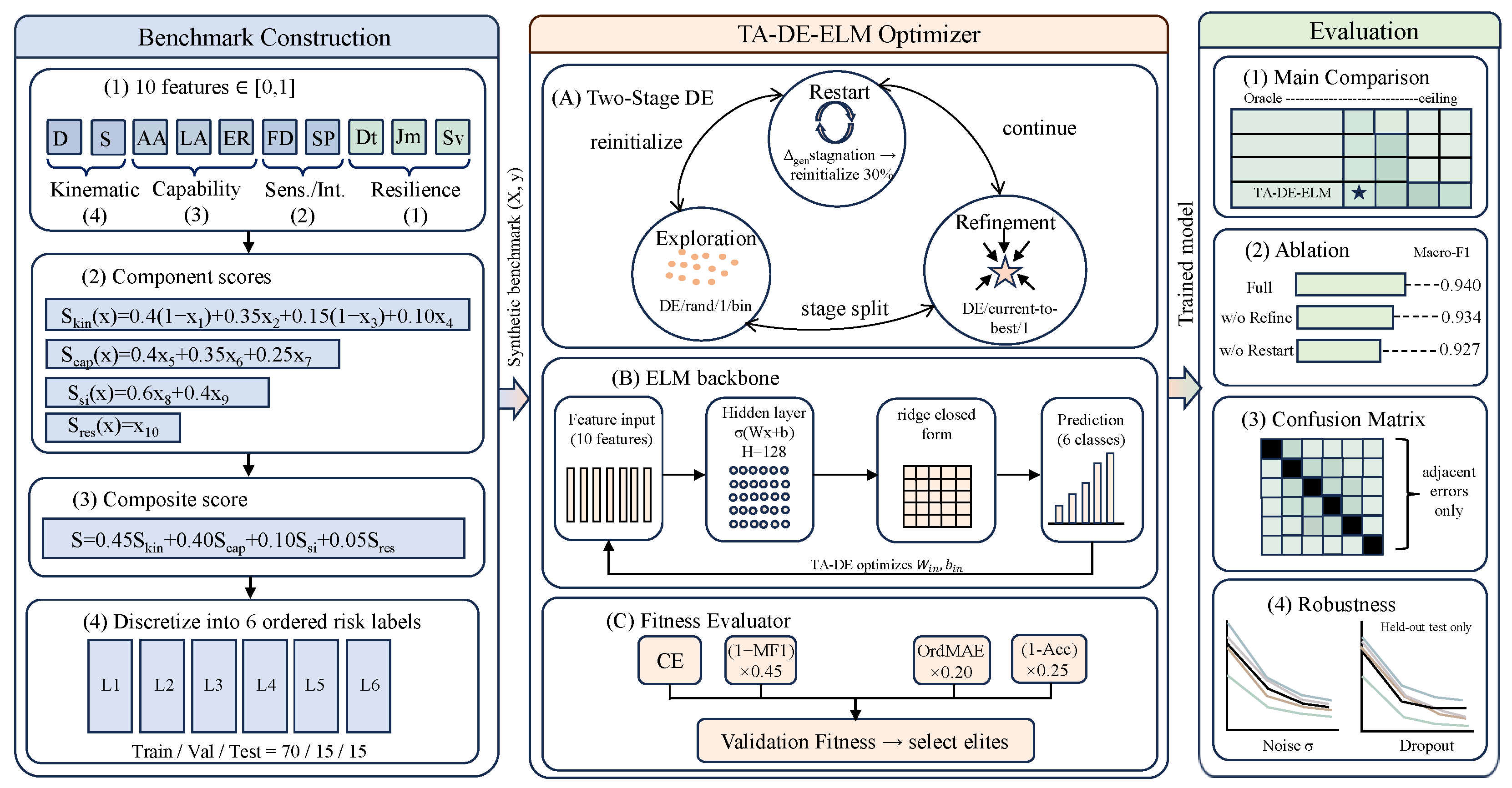
This section presents the proposed ordered-risk assessment framework as a controlled synthetic benchmark pipeline. As illustrated in Figure 1, the architecture consists of three coordinated modules: (1) an expert-rule-guided benchmark, which generates normalized synthetic samples from kinematic and attribute rules under fixed prior assumptions; (2) the TA-DE-ELM optimizer, which performs stage-wise differential evolution to optimize the ELM input parameters while retaining a closed-form output layer; and (3) an evaluation protocol, which combines the finite-budget main comparison, statistical testing, component ablation, and ordered-error metrics.

3.1. Expert-Rule-Guided Risk Data Generation

Obtaining large-scale labeled real-world data is often infeasible because of confidentiality constraints and the rarity of critical events. To address this limitation, we designed an expert-rule-guided data-generation mechanism that synthesizes normalized entities according to explicit risk-scoring assumptions. This mechanism should not be interpreted as a first-principles physical simulator or a replacement for application-specific validation. Instead, it provides a transparent, auditable benchmark in which the assumed monotonic relations among proximity, maneuvering state, capability descriptors, sensing/interference activity, and resilience are fixed before model training.

Each synthetic entity is represented by a normalized feature vector $\mathbf{x}\in {[0,1]}^{10}$:

$$\begin{array}{cc}\hfill \mathbf{x}=[x_1,\dots ,x_{10}]=& [\mathrm{distance},\mathrm{speed},\mathrm{approach}\mathrm{angle},\mathrm{lateral}\mathrm{acceleration},\hfill \\ \hfill & \mathrm{operating}\mathrm{range},\mathrm{capability}\mathrm{intensity},\mathrm{precision}\mathrm{index},\hfill \\ \hfill & \mathrm{sensing}\mathrm{level},\mathrm{interference}\mathrm{level},\mathrm{resilience}\mathrm{descriptor}]\hfill \end{array}$$

(1)

The ten factors are selected to cover four interpretable information groups: kinematic state, capability descriptors, sensing/interference activity, and resilience. This organization follows five design principles commonly used when constructing indicator systems: coverage of key entity attributes, hierarchy across information groups, measurable feature definitions, physical plausibility, and comparability after normalization.

Table 1. Indicator grouping, feature semantics, and risk-oriented mappings used in the expert-rule-guided generator.

Indicator Group	Included Variables	Risk-Oriented Mapping	Risk-Scoring Role
Kinematic state	Distance, speed, approach angle, and lateral acceleration	$1-{\tilde{x}}_1$, ${\tilde{x}}_2$, $1-{\tilde{x}}_3$, ${\tilde{x}}_4$	Captures proximity, approach tendency, and maneuvering intensity.
Capability descriptors	Operating range, capability intensity, and precision index	${\tilde{x}}_5$, ${\tilde{x}}_6$, ${\tilde{x}}_7$	Represents normalized capability-related attributes that increase the assigned risk score under expert-defined assumptions.
Sensing/interference activity	Sensing level and interference level	${\tilde{x}}_8$, ${\tilde{x}}_9$	Represents sensing-related information and interference pressure as normalized benchmark indicators.
Resilience	Resilience descriptor	${\tilde{x}}_{10}$	Represents persistence-related attributes that increase the assigned risk score under the benchmark rules.

summarizes the resulting indicator grouping, feature semantics, and risk-oriented mappings before the mathematical generator is defined. The directions encode prior risk-scoring assumptions, not learned causal laws.

Table 2. Correspondence between the controlled synthetic benchmark components and abstract assessment properties.

Benchmark Component	Assessment Motivation	What Is Represented	Main Simplification
Kinematic factors (distance, speed, approach angle, lateral acceleration)	Response urgency and maneuvering complexity	Proximity, approach tendency, short-term maneuvering intensity, and time-sensitive prioritization cues	No continuous trajectory propagation, environmental constraint, or adaptive motion policy is simulated.
Capability factors (operating range, capability intensity, precision index)	Capability-related risk contribution	Normalized capability descriptors under expert-defined assumptions	No domain-specific effect, resource-use, or outcome model is included.
Sensing/interference factors (sensing level, interference level)	Sensing and interference pressure	Sensing-related information and interference pressure as normalized benchmark indicators	Detailed sensor-chain and interference processes are simplified to normalized indicators.
Resilience descriptor	Persistence-related risk contribution	Relative resilience represented as a normalized benchmark indicator	No field-level degradation, recovery, or platform-level resilience simulation is performed.
Boundary uncertainty and feature degradation	Label ambiguity and sensing uncertainty	Boundary-proximal label noise, additive feature noise, and structured feature-group dropout	Perturbations are controlled stress tests, not a high-fidelity model of sensor latency, clutter, occlusion, or domain shift.

further clarifies which abstract properties are represented by this controlled synthetic simulation and which aspects remain simplified.

The choice of these ten indicators is consistent with the broader assessment literature, as summarized in

Table 3. Literature-level comparison of ordered-risk indicator coverage. ✓ denotes indicator categories explicitly used; ○ denotes partial or derived coverage; numbers in parentheses indicate the number of variables used in each indicator category.

Study	Kinem.	Capab.	Sens./Int.	Resil.	Features
Zhao et al. [29]	✓	✓	✓	○	9
Pires and Guimarães [17]	✓	–	–	–	4
Wu et al. [16]	✓	✓	–	–	7
Yin et al. [36]	✓	✓	–	–	4
Luo et al. [5]	✓	✓	○	–	6
This work	✓ (4)	✓ (3)	✓ (2)	✓ (1)	10

. Most related studies include kinematic, capability, and sensing-activity features; the present work additionally includes lateral acceleration and resilience to support the four-group decomposition required by the scoring generator.

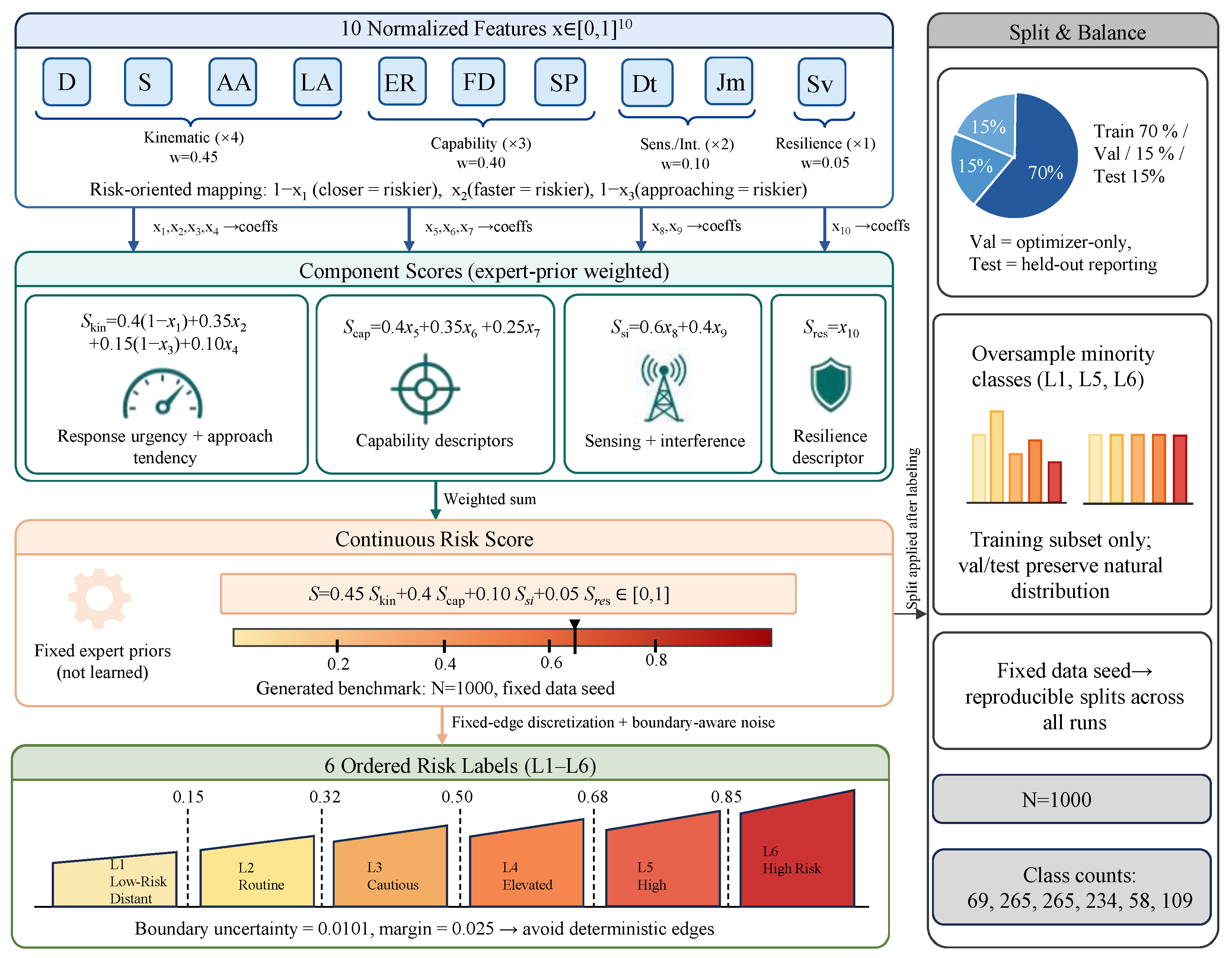
Raw features are first normalized by fixed physical bounds to obtain $\tilde{\mathbf{x}}\in {[0,1]}^{10}$. We then compute four interpretable component scores:

$$\begin{array}{cc}\hfill S_{\mathrm{kin}}\left(\tilde{\mathbf{x}}\right)& =0.4(1-{\tilde{x}}_1)+0.35{\tilde{x}}_2+0.15(1-{\tilde{x}}_3)+0.10{\tilde{x}}_4,\hfill \end{array}$$

(2)

$$\begin{array}{cc}\hfill S_{\mathrm{cap}}\left(\tilde{\mathbf{x}}\right)& =0.4{\tilde{x}}_5+0.35{\tilde{x}}_6+0.25{\tilde{x}}_7,\hfill \end{array}$$

(3)

$$\begin{array}{cc}\hfill S_{\mathrm{si}}\left(\tilde{\mathbf{x}}\right)& =0.6{\tilde{x}}_8+0.4{\tilde{x}}_9,\hfill \end{array}$$

(4)

$$\begin{array}{cc}\hfill S_{\mathrm{res}}\left(\tilde{\mathbf{x}}\right)& ={\tilde{x}}_{10}.\hfill \end{array}$$

(5)

The final continuous risk score is

$$S\left(\tilde{\mathbf{x}}\right)=0.45S_{\mathrm{kin}}+0.40S_{\mathrm{cap}}+0.10S_{\mathrm{si}}+0.05S_{\mathrm{res}},$$

(6)

with $S\left(\tilde{\mathbf{x}}\right)\in [0,1]$. Here, the subscripts “si” and “res” denote sensing/interference and resilience, respectively. The coefficients in the component scores and in the final aggregation are expert-prior weights fixed before model training. They encode the assumed relative importance of the four information groups in this controlled benchmark; they are not estimated from the test labels and are not claimed as universal physical constants.

Table 4. Effective feature-level prior-weight allocation in the expert-rule-guided generator.

Feature	Group	Effective Weight	Risk Score Term
Distance	Kinematic state	$0.1800$	$1-{\tilde{x}}_1$
Speed	Kinematic state	$0.1575$	${\tilde{x}}_2$
Approach angle	Kinematic state	$0.0675$	$1-{\tilde{x}}_3$
Lateral acceleration	Kinematic state	$0.0450$	${\tilde{x}}_4$
Operating range	Capability descriptors	$0.1600$	${\tilde{x}}_5$
Capability intensity	Capability descriptors	$0.1400$	${\tilde{x}}_6$
Precision index	Capability descriptors	$0.1000$	${\tilde{x}}_7$
Sensing level	Sensing/interference activity	$0.0600$	${\tilde{x}}_8$
Interference level	Sensing/interference activity	$0.0400$	${\tilde{x}}_9$
Resilience descriptor	Resilience	$0.0500$	${\tilde{x}}_{10}$

reports the resulting effective feature-level weights after multiplying each component coefficient by its group coefficient.

Prior-Weight Sensitivity

The expert-prior weights in the component scores and the group aggregation are fixed before model training and do not adapt to data. To verify that the resulting risk labels are not hypersensitive to small variations in these weights, we perturbed all coefficients simultaneously by $\pm 10\%$, $\pm 20\%$, and $\pm 30\%$ (with random sign draws repeated across 20 trials), re-normalized, and measured the Jensen–Shannon divergence between the perturbed and baseline label distributions on 2000 generated samples. The resulting JS-divergence values were $2.4\times {10}^{-5}$, $1.3\times {10}^{-4}$, and $3.4\times {10}^{-4}$, respectively—all below ${10}^{-3}$. This confirms that the six-level label distribution is stable under moderate weight uncertainty and that the benchmark does not rely on a single fragile prior parameterization. Similarly, shifting individual score edges by $\pm 0.02$ changes fewer than $8\%$ of labels, while a uniform shift in all five edges by $-0.02$ changes approximately $12\%$ of labels. Edge sensitivity is confined to samples near class boundaries, consistent with the ordered-discretization design. The fixed edges should therefore be treated as benchmark definitions rather than general-purpose decision thresholds.

To obtain ordered-risk levels, we discretize $S\left(\tilde{\mathbf{x}}\right)$ with fixed edges

$$\mathbf{e}=(0.15,0.32,0.50,0.68,0.85),$$

(7)

and define the labels as

$$y\in \{1,\dots ,6\},y=1+{\displaystyle \sum _{k=1}^5}\mathbb{I}\left(S\left(\tilde{\mathbf{x}}\right)>e_k\right).$$

(8)

The thresholds are also fixed before model optimization to span six ordered-risk levels, from low to high risk. In particular, the $0.68$ edge is the boundary between risk levels 4 and 5 in this fixed risk-level partition; it is not a tuned switching point selected to improve the classifier performance. Consequently, the experiments evaluated whether learning models can reproduce and generalize the structured risk-level mapping under held-out splits and a fixed finite-budget protocol, rather than validating application-specific decision thresholds. The complete construction chain from ten features to four component scores, one continuous risk score, six ordered labels, and the split-and-balance protocol is summarized in Figure 2.

3.2. Extreme Learning Machine (ELM)

An extreme learning machine (ELM) is a single-hidden-layer feedforward neural network with fast training and good generalization, and recent work has continued to study its theoretical assumptions, pseudo-inverse variants, hybrid architectures, and optimized implementations [30,38,39,40,41]. For N samples ${\left\{({\mathbf{x}}_i,y_i)\right\}}_{i=1}^N$ with ${\mathbf{x}}_i\in {\mathbb{R}}^d$ and $y_i\in \{1,\dots ,C\}$, the hidden-layer output is

$${\mathbf{h}}_i=g(\mathbf{W}{\mathbf{x}}_i+\mathbf{b}),\mathbf{W}\in {\mathbb{R}}^{H\times d},\mathbf{b}\in {\mathbb{R}}^H$$

(9)

where H is the number of hidden nodes and $g(·)$ is the activation function. Stacking all samples yields $\mathbf{H}=[{\mathbf{h}}_1,\dots ,{\mathbf{h}}_N]\in {\mathbb{R}}^{H\times N}$. The output weights $\mathbf{B}\in {\mathbb{R}}^{H\times C}$ are obtained by ridge regression:

$$\widehat{\mathbf{B}}=\arg \underset{\mathbf{B}}{\min }\parallel {\mathbf{B}}^{\top }{\mathbf{H}-\mathbf{T}\parallel }_F^2+\lambda {\parallel \mathbf{B}\parallel }_F^2$$

(10)

with the closed-form solution

$$\widehat{\mathbf{B}}={(\mathbf{H}{\mathbf{H}}^{\top }+\lambda \mathbf{I})}^{-1}\mathbf{H}{\mathbf{T}}^{\top }$$

(11)

where $\mathbf{T}\in {\mathbb{R}}^{C\times N}$ is the one-hot label matrix. The prediction uses logits ${\mathbf{z}}_i={\widehat{\mathbf{B}}}^{\top }{\mathbf{h}}_i$ and ${\widehat{y}}_i=1+\arg {\max }_c{z}_{i,c}$.

In our implementation, the optimization variable is $\theta =(\mathbf{W},\mathbf{b})\in {\mathbb{R}}^{Hd+H}$ with box bounds ${[-1,1]}^{Hd+H}$, whereas the output weights are solved analytically using a closed-form ridge solution.

Instead of sampling $\mathbf{W}$ and $\mathbf{b}$ randomly, we optimized them using metaheuristics to reduce the initialization sensitivity while still solving $\mathbf{B}$ analytically.

3.3. Two-Stage Adaptive Differential Evolution (TA-DE)

Standard differential evolution [31] may still converge prematurely when optimizing high-dimensional ELM input parameters. We therefore adopted a two-stage adaptive differential evolution (TA-DE) strategy that explicitly balances exploration and exploitation.

3.3.1. Two-Stage Search Strategy

In each iteration, the population is updated through two coordinated stages:

• Stage 1 (exploration): Differential mutation/crossover emphasizes a broad search coverage to avoid early stagnation.
• Stage 2 (refinement): Adaptive control and elitist refinement improve the local convergence quality around promising regions.
• Stagnation restart: When improvement stalls, a fraction of individuals is reinitialized to recover diversity.

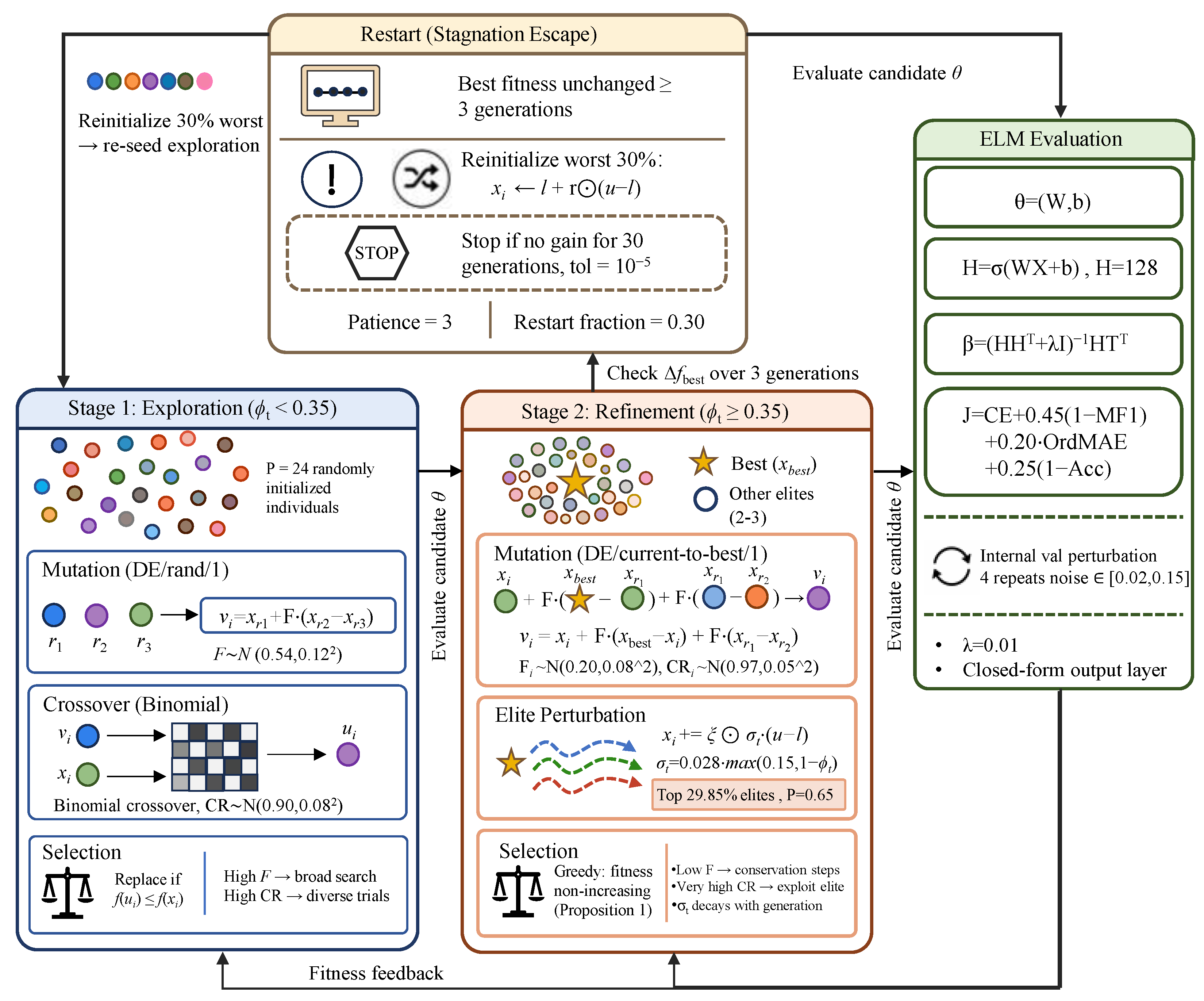
The resulting TA-DE search mechanism is illustrated in Figure 3, which makes explicit the stage switch, the stagnation-triggered restart, and the closed-form ELM evaluation loop used to score candidate input parameters.

3.3.2. Adaptive Update Mechanisms

Different update rules are applied across stages. Let ${\varphi }_t=t/T$ denote the normalized generation index, where T is the maximal generation. The refinement stage starts when ${\varphi }_t\ge \rho$, where $\rho \in (0,1)$ is the stage-split parameter.

1. Exploration stage update: Classical DE/rand/1 mutation and binomial crossover are used:

$${\mathbf{v}}_i^{\left(t\right)}={\mathbf{x}}_{r_1}^{\left(t\right)}+F_i^{\left(t\right)}\left({\mathbf{x}}_{r_2}^{\left(t\right)}-{\mathbf{x}}_{r_3}^{\left(t\right)}\right),{\mathbf{u}}_i^{\left(t\right)}=\mathrm{BinCross}\left({\mathbf{v}}_i^{\left(t\right)},{\mathbf{x}}_i^{\left(t\right)},C{R}_i^{\left(t\right)}\right),$$

(12)

where $F_i^{\left(t\right)}\sim \mathcal{N}(F,{0.12}^2)$ and $C{R}_i^{\left(t\right)}\sim \mathcal{N}(CR,{0.08}^2)$ are clipped into valid ranges.

2. Refinement stage update: In late iterations, current-to-best style mutation and tighter adaptive parameters are used:

$${\mathbf{v}}_i^{\left(t\right)}={\mathbf{x}}_i^{\left(t\right)}+F_i^{\left(t\right)}\left({\mathbf{x}}_{\mathrm{best}}^{\left(t\right)}-{\mathbf{x}}_i^{\left(t\right)}\right)+F_i^{\left(t\right)}\left({\mathbf{x}}_{r_1}^{\left(t\right)}-{\mathbf{x}}_{r_2}^{\left(t\right)}\right),$$

(13)

with $F_i^{\left(t\right)}\sim \mathcal{N}(F_{\mathrm{refine}},{0.08}^2)$ and $C{R}_i^{\left(t\right)}\sim \mathcal{N}(C{R}_{\mathrm{refine}},{0.05}^2)$. In addition, elite individuals receive Gaussian local refinement:

$${\mathbf{x}}_i^{\left(t\right)}\leftarrow {\mathbf{x}}_i^{\left(t\right)}+\mathit{\xi }\odot \left({\sigma }_t(\mathbf{u}-\mathbf{l})\right),{\sigma }_t={\sigma }_0\max (0.15,1-{\varphi }_t),\mathit{\xi }\sim \mathcal{N}(\mathbf{0},\mathbf{I}).$$

(14)

3. Restart mechanism: If the best fitness does not improve for a patience window after entering refinement, a fraction of worst individuals is reinitialized:

$${\mathbf{x}}_i\leftarrow \mathbf{l}+\mathbf{r}\odot (\mathbf{u}-\mathbf{l})$$

(15)

where $\mathbf{l},\mathbf{u}$ are search bounds and $\mathbf{r}\sim \mathcal{U}(0,1)$.

3.4. Validation Objective Function

For each candidate $\theta =(\mathbf{W},\mathbf{b})$, we fit $\widehat{\mathbf{B}}$ on a fitting subset and evaluate the candidate on a validation subset. The validation objective is

$$J\left(\theta \right)=\mathrm{CE}+w_f(1-\mathrm{F}{1}_{\mathrm{macro}})+w_o{\mathrm{MAE}}_{\mathrm{ord}}+w_a(1-\mathrm{Acc}),$$

(16)

where $(w_f,w_o,w_a)=(0.45,0.20,0.25)$ and

$${\mathrm{MAE}}_{\mathrm{ord}}={\displaystyle \frac{1}{C-1}}·{\displaystyle \frac{1}{N_{\mathrm{val}}}}{\displaystyle \sum _{i=1}^{N_{\mathrm{val}}}}\left|{\widehat{y}}_i-y_i\right|.$$

(17)

This design jointly promotes probabilistic separation, class-balanced recognition, risk-order consistency, and overall predictive accuracy. During TA-DE candidate scoring only, the validation subset is also evaluated through a small set of perturbed validation replicas. This internal validation augmentation discourages candidate solutions that are highly sensitive to minor feature disturbances or group-wise missingness, but it is not reported as a standalone robustness experiment.

3.4.1. Core Hyperparameters

The core symbols follow the formulation above; $\mathbf{x}\in {\mathbb{R}}^d$ denotes the normalized input vector, $y\in \{1,\dots ,C\}$ the ordered-risk label, $\theta =(\mathbf{W},\mathbf{b})$ the TA-DE search variable, and $J\left(\theta \right)$ the validation objective.

Table 5. TA-DE-ELM hyperparameters used in the finalized unified-budget main comparison.

Item	Value	Role
Population size P	24	Number of candidate vectors per generation.
Max generation T	60	Upper bound of optimization iterations.
ELM hidden size H	128	Representation capacity of ELM hidden layer.
$F,CR$	$0.5442,0.9046$	Exploration-stage mutation and crossover.
$F_{\mathrm{refine}},C{R}_{\mathrm{refine}}$	$0.2000,0.9700$	Refinement-stage mutation and crossover.
Stage split $\rho$	$0.3500$	Refinement starts when ${\varphi }_t\ge \rho$.
Elite fraction	$0.2985$	Top candidates used for local refinement.
Refine probability	$0.6500$	Probability of elite local Gaussian refinement.
Refine sigma	$0.0280$	Local refinement scale factor.
Restart patience	3	Stall window before restart trigger.
Restart fraction	$0.3000$	Worst-candidate portion to reinitialize.
Validation regularization $\lambda$	$0.01$	Ridge penalty used in candidate scoring.
Validation perturbation repeats	4	Number of internal validation replicas used in TA-DE candidate scoring.
Feature-perturbation range	$[0.0229,0.1532]$	Small validation-only disturbance range used by the optimizer.
Group-missing range	$[0.0420,0.1240]$	Validation-only group-dropout range used by the optimizer.
Early-stop patience	30	Consecutive no-improvement generations for stop.
Early-stop tolerance	${10}^{-5}$	Improvement threshold for stall counting.

reports the finalized hyperparameter settings used in the unified-budget comparison.

The numerical settings in Table 5, including the stage split $\rho =0.3500$, were selected through a directed validation search under the unified finite budget, and were not tuned on the test set. All values were rounded to four decimal places where the search granularity supported it. They should not be interpreted as physical constants. In practice, $\rho$ controls when the optimizer changes from broad population exploration to local refinement; the early transition used here gives the refinement and restart mechanisms enough budget to act under the deliberately compact $P=24$, $T=60$ protocol.

3.4.2. Monotonic Best-Value Property

Proposition 1.

Let $f_t^{\star }$ be the best fitness after generation t. Under the greedy replacement used in TA-DE, the sequence $\left\{f_t^{\star }\right\}$ is non-increasing.

Proof. 

In each trial update, a candidate replaces the current individual only when $f_{\mathrm{new}}\le f_{\mathrm{old}}$. Therefore, every accepted replacement cannot increase the population’s best value. Elite local refinement is also accepted only when the fitness is not worse, and restart updates immediately re-evaluate and retain the current best if no better candidate appears. Hence, after each generation, $f_{t+1}^{\star }\le f_t^{\star }$.    □

3.5. Algorithm Summary and Complexity

The overall optimization, training, and inference pipeline is formalized in Algorithm 1.

Algorithm 1 TA-DE-ELM training and inference pipeline.

Input  Dataset $\mathcal{D}={\left\{({\mathbf{x}}_i,y_i)\right\}}_{i=1}^N$, hidden size H, population size P, maximum generation T, stage split $\rho$, search bounds $[\mathbf{l},\mathbf{u}]$, and validation weights $(w_f,w_o,w_a)$. Output  Optimized ELM parameters $({\mathbf{W}}^{\star },{\mathbf{b}}^{\star },{\mathbf{B}}^{\star })$ and predicted ordered-risk labels $\widehat{y}$. 1. Split  Partition $\mathcal{D}$ into training, validation, and test subsets; scale features to $[-1,1]$ with statistics fitted on the training subset. 2. Initialize  Generate P candidate vectors ${\theta }_i=({\mathbf{W}}_i,{\mathbf{b}}_i)$ within $[\mathbf{l},\mathbf{u}]$; for each candidate, solve ${\mathbf{B}}_i$ by the ELM closed form and evaluate $J\left({\theta }_i\right)$ on the validation subset. 3. Search  For generation $t=1,\dots ,T$, compute ${\varphi }_t=t/T$ and select the exploration update when ${\varphi }_t<\rho$ or the refinement update when ${\varphi }_t\ge \rho$. 4. Adapt  Sample candidate-specific $(F_i,C{R}_i)$, perform mutation and crossover, solve the candidate ELM output weights analytically, and accept the trial vector only if it does not increase the validation objective. 5. Refine  In the refinement stage, apply an elite Gaussian local search with greedy acceptance; if the best value stalls for the patience window, reinitialize the worst candidate fraction and keep the current best solution. 6. Retrain  Select ${\theta }^{\star }=({\mathbf{W}}^{\star },{\mathbf{b}}^{\star })$ with the lowest validation objective and recompute ${\mathbf{B}}^{\star }$ on the final training data using the closed-form ridge solution. 7. Infer  For each test sample, compute hidden activations, logits $\mathbf{z}={\left({\mathbf{B}}^{\star }\right)}^{\top }g({\mathbf{W}}^{\star }\mathbf{x}+{\mathbf{b}}^{\star })$, and the ordered-risk prediction $\widehat{y}=1+\arg {\max }_c{z}_c$.

Let N be the number of fit samples, H the hidden size, d the input dimension, C the number of classes, and P the population size. One fitness evaluation costs $\mathcal{O}(HdN+H^{2}N+H^3+CN)$ due to hidden activation construction, ridge-system formation/solve, and validation scoring. One TA-DE generation requires P primary evaluations plus bounded extra evaluations from elite refinement/restart, so the per-generation complexity remains $\mathcal{O}\left(P(HdN+H^{2}N+H^3+CN)\right)$. The total cost scales linearly with effective generations before early stopping. After $(\mathbf{W},\mathbf{b})$ has been selected, online inference uses the same ELM forward computation and closed-form output layer as other optimized ELM variants. Computational-cost measurements are reported after the main evaluation results; all ELM-family models share the same hidden-layer size ($H=128$) and differ only in optimizer overhead, which is modest relative to the fitness evaluation cost. The complete evaluation protocol is presented in Section 4.

4. Experimental Design and Analysis

This section evaluates whether TA-DE-ELM improves six-level ordered-risk classification under a fixed expert-rule-guided benchmark and a unified finite-optimization budget. The experimental evidence is organized around five questions: (1) whether TA-DE-ELM outperforms ELM-family baselines on held-out test data, (2) whether it remains competitive against traditional scoring and ranking references, (3) whether the optimization trace supports faster and stronger validation convergence under a common evaluator, (4) whether the proposed refinement and restart mechanisms contribute to the observed performance, and (5) whether TA-DE-ELM maintains stable risk-order predictions under feature degradation and group dropout. The Oracle baseline and prior-weight sensitivity check in Section 3.1 further bound the benchmark’s self-consistency and parameter stability.

4.1. Dataset and Experimental Protocol

We adopted the expert-rule-guided synthetic benchmark generated by the kinematic and attribute rules in Section 3.1. Each sample contained $d=10$ normalized features in $[0,1]$ and was assigned to one of $L=6$ ordered-risk levels via fixed-edge discretization of the continuous risk score. The reported benchmark contained 1000 samples generated with the fixed data seed used in the reproducible code configuration. The resulting class counts were 69, 265, 265, 234, 58, and 109 for risk levels 1–6, respectively. The four feature groups used in the experiments followed the indicator semantics summarized in Table 1. The label distribution was intentionally not forced to be uniform because the fixed-score edges induced fewer extreme low- and high-risk cases than middle-risk cases. To avoid training bias from this imbalance, random oversampling was applied only to the training subset; the validation and test subsets preserved the held-out distribution.

The train/validation/test split ratio was fixed to $70\%/15\%/15\%$. The validation subset was used only inside optimization for candidate selection, while the test subset was strictly held out for final reporting. All the reported main-comparison and ablation values are the mean ± std over five repeated optimization runs on the same benchmark split, with paired optimizer seeds across the compared methods. Raw normalized features were used for all methods. The data generator used a label-boundary uncertainty of $0.0101$ and a boundary margin of $0.025$ to avoid overly deterministic class boundaries near fixed-score edges. Unless otherwise stated, the ELM-family models used a hidden size $H=128$, a population size $P=24$, and maximum generation $T=60$.

4.2. Compared Methods and Implementation Details

In the main comparative benchmark, we compared TA-DE-ELM with standard ELM and three metaheuristic-optimized ELM variants—PSO-ELM, DE-ELM, and GA-ELM—following the representative literature on ELM classifiers and metaheuristic-optimized ELM variants [30,31,38,39,41,42,43,44]. All ELM-family baselines share the same backbone, activation function, preprocessing, and closed-form output-weight solution; only the input-weight and hidden-bias initialization or optimization strategy differs. This design isolates whether the two-stage adaptive DE mechanism improves the ELM backbone under budget parity.

Within each benchmark, all evolutionary optimizers ran under the same population size and maximum generation budget. TA-DE-ELM followed the validation objective in Section 3.4. The stochastic components were controlled by explicit split and optimization seeds to guarantee reproducibility. Run-wise differences against TA-DE-ELM were computed on paired repeated runs; for the current five-run protocol, paired t-tests are reported to summarize these differences.

For the non-ELM references, Entropy-GRA and RF-GRA used entropy weights and random-forest feature-importance weights, respectively, with a common GRA scorer, whereas CRITIC-TOPSIS and CRITIC-VIKOR used CRITIC-style weights with the corresponding ranking rule. The latter weights combined normalized feature dispersion with intercriterion conflict measured from absolute feature correlations; VIKOR balanced group utility and individual regret with $v=0.5$ [33,34]. Specifically, RF-GRA fitted a 300-tree random forest to the training split, normalized its feature-importance values, and used them as GRA weights [32,35]. Validation scores were used to calibrate the six-class decision edges; the test split remained held out.

As a theoretical ceiling, we also report an Oracle that applies the noise-free scoring function $S\left(\tilde{\mathbf{x}}\right)$ directly as a classifier (discretizes the clean score via the fixed edges without passing through the ELM). Because the generated labels already encode $S\left(\tilde{\mathbf{x}}\right)$ plus small boundary-aware noise ($0.0101$), the Oracle quantifies the irreducible error from label noise and establishes an upper bound for any learned model on this benchmark. It does not represent a practical competitor; it confirms label self-consistency.

4.3. Evaluation Metrics

To evaluate the performance of the proposed method, we report the accuracy, macro-F1, quadratic weighted kappa (QWK), and ordinal MAE on held-out tests. Let K denote the number of classes ($K=6$ in this work), N the number of test samples, $C_{ij}$ the confusion-matrix count from true class i to predicted class j, and $y_n,{\widehat{y}}_n\in \{1,\dots ,K\}$ the true and predicted labels for sample n. The metrics are defined as

$$\begin{array}{cc}\hfill \mathrm{Accuracy}& ={\displaystyle \frac{1}{N}}{\displaystyle \sum _{n=1}^N}\mathbb{I}\left({\widehat{y}}_n=y_n\right),\hfill \\ \hfill \mathrm{Ordinal}\mathrm{MAE}& ={\displaystyle \frac{1}{N}}{\displaystyle \sum _{n=1}^N}{\displaystyle \frac{\left|{\widehat{y}}_n-y_n\right|}{K-1}}.\hfill \end{array}$$

(18)

$$\mathrm{Macro}\text{-}\mathrm{F1}={\displaystyle \frac{1}{K}}{\displaystyle \sum _{k=1}^K}{\displaystyle \frac{2P_k{R}_k}{P_k+R_k}},P_k={\displaystyle \frac{C_{kk}}{{\sum }_{i=1}^K{C}_{ik}}},R_k={\displaystyle \frac{C_{kk}}{{\sum }_{j=1}^K{C}_{kj}}}.$$

(19)

$$\mathrm{QWK}=1-{\displaystyle \frac{{\sum }_{i=1}^K{\sum }_{j=1}^K{W}_{ij}{O}_{ij}}{{\sum }_{i=1}^K{\sum }_{j=1}^K{W}_{ij}{E}_{ij}}},W_{ij}={\displaystyle \frac{{(i-j)}^2}{{(K-1)}^2}}.$$

(20)

where $O_{ij}=C_{ij}/N$ and $E_{ij}$ is the expected disagreement matrix induced by empirical class marginals. Because the risk levels are ordered, QWK and ordinal MAE are treated as primary rank-consistency indicators in addition to accuracy and macro-F1.

4.4. Overall Performance Comparison

This experiment examined whether TA-DE improves the accuracy–stability trade-off under strict budget parity.

Table 6. Main performance comparison on the six-level risk dataset (mean ± std over five repeated runs under the finalized finite-budget protocol). The Oracle row reports the deterministic rule ceiling obtained by applying the noise-free scoring function directly as a classifier; it does not involve model training. The compared baselines follow the representative ELM and metaheuristic-optimized ELM literature [30,31,38,39,41,42,43,44]. Bold values denote the best learned-model results; ↓ indicates that lower values are better.

Method	Accuracy	Macro-F1	QWK	Ordinal MAE ↓
Oracle (rule ceiling)	$0.9934$	$0.9935$	$0.9989$	$0.0013$
TA-DE-ELM (ours)	$\mathbf{0.9404}\pm \mathbf{0.0084}$	$\mathbf{0.9396}\pm \mathbf{0.0084}$	$\mathbf{0.9899}\pm \mathbf{0.0014}$	$\mathbf{0.0119}\pm \mathbf{0.0017}$
DE-ELM	$0.9192\pm 0.0097$	$0.9180\pm 0.0097$	$0.9864\pm 0.0017$	$0.0162\pm 0.0019$
PSO-ELM	$0.8570\pm 0.0176$	$0.8536\pm 0.0177$	$0.9761\pm 0.0030$	$0.0286\pm 0.0035$
GA-ELM	$0.8543\pm 0.0173$	$0.8508\pm 0.0178$	$0.9757\pm 0.0029$	$0.0291\pm 0.0035$
ELM	$0.8397\pm 0.0077$	$0.8352\pm 0.0083$	$0.9733\pm 0.0013$	$0.0321\pm 0.0015$

reports the full comparison. The Oracle row establishes a deterministic rule ceiling (accuracy, $0.9934$; macro-F1, $0.9935$; QWK, $0.9989$), confirming that the scoring-function labels are internally consistent. TA-DE-ELM led all learned ELM-family methods in accuracy, macro-F1, QWK, and ordinal MAE. Relative to vanilla ELM, TA-DE-ELM increased macro-F1 from $0.8352$ to $0.9396$ and reduced ordinal MAE from $0.0321$ to $0.0119$. Relative to the closest optimized baseline, DE-ELM, TA-DE-ELM improved accuracy by $+0.0212$ ($p=0.0121$), macro-F1 by $+0.0216$ ($p=0.0116$), and QWK by $+0.0035$ ($p=0.0126$). The accuracy gap between TA-DE-ELM ($0.9404$) and the Oracle ceiling ($0.9934$) was $0.0530$, leaving measurable headroom to the noise-free rule ceiling. The main claim is therefore a consistent finite-budget improvement over ELM-family baselines, not order-of-magnitude superiority.

Beyond the ELM-family baselines, we evaluated four traditional scoring and ranking references: Entropy-GRA, CRITIC-TOPSIS, CRITIC-VIKOR, and RF-GRA. These methods used the same train/validation/test split and converted their continuous or ranking scores into the six fixed risk levels for held-out evaluation. As shown in

Table 7. Traditional scoring and ranking references on the same six-level risk benchmark (mean ± std over repeated runs). These methods provide non-ELM reference baselines in addition to the ELM-family comparison. Bold values denote the best results for the primary performance metrics; ↓ indicates that lower values are better.

Method	Accuracy	Macro-F1	QWK	Ordinal MAE ↓	Severe Underest. ↓
TA-DE-ELM (ours)	$\mathbf{0.9404}\pm \mathbf{0.0084}$	$\mathbf{0.9396}\pm \mathbf{0.0084}$	$\mathbf{0.9899}\pm \mathbf{0.0014}$	$\mathbf{0.0119}\pm \mathbf{0.0017}$	$0.0000\pm 0.0000$
RF-GRA	$0.9117\pm 0.0219$	$0.9068\pm 0.0241$	$0.9776\pm 0.0051$	$0.0177\pm 0.0044$	$0.0000\pm 0.0000$
Entropy-GRA	$0.9029\pm 0.0343$	$0.8879\pm 0.0330$	$0.9758\pm 0.0078$	$0.0194\pm 0.0069$	$0.0000\pm 0.0000$
CRITIC-TOPSIS	$0.5607\pm 0.0380$	$0.5935\pm 0.0566$	$0.8606\pm 0.0235$	$0.0958\pm 0.0124$	$0.0264\pm 0.0187$
CRITIC-VIKOR	$0.5320\pm 0.0298$	$0.5718\pm 0.0445$	$0.8315\pm 0.0207$	$0.1073\pm 0.0089$	$0.0627\pm 0.0123$

, RF-GRA and Entropy-GRA provided competitive interpretable references. TA-DE-ELM nevertheless achieved higher macro-F1 and lower ordinal MAE under the same benchmark. This comparison tests whether nonlinear ELM optimization improves held-out discrimination while retaining the transparent fixed-score benchmark.

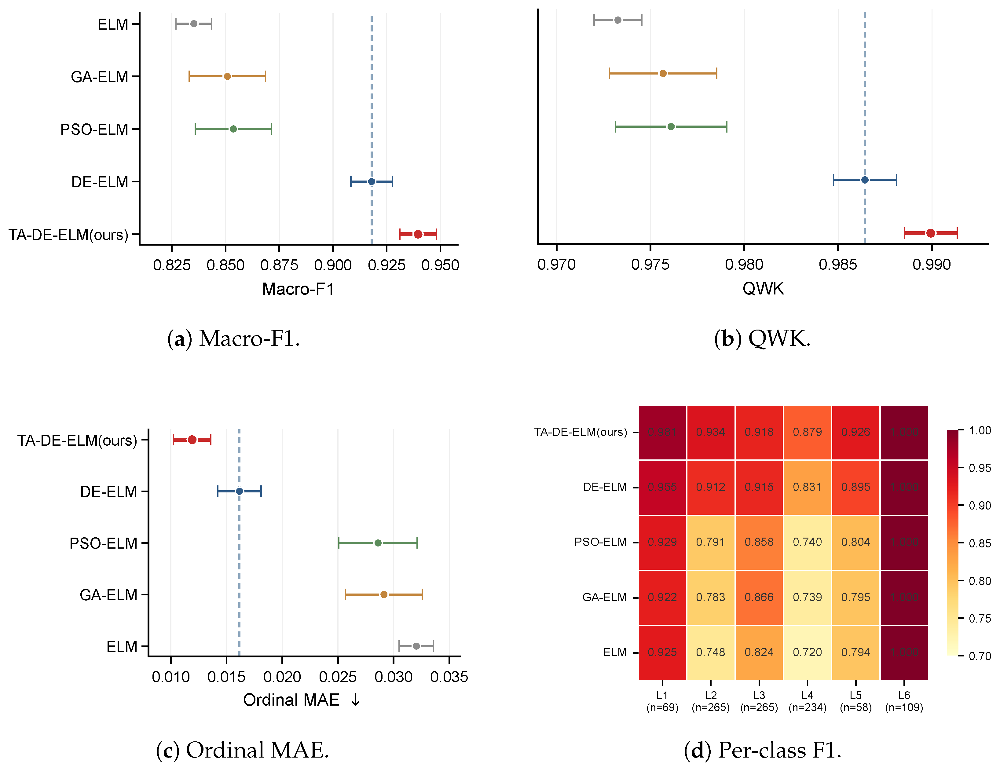
Figure 4 shows the main comparative evidence in a $2\times 2$ layout: panels (a–c) report the macro-F1, QWK, and ordinal MAE as the mean ± std across five repeated runs, with the DE-ELM reference line marked in each panel; panel (d) provides a per-class F1 heatmap across all five ELM-family models, with class sample counts annotated on the x-axis. TA-DE-ELM (ours) is highlighted consistently across all panels.

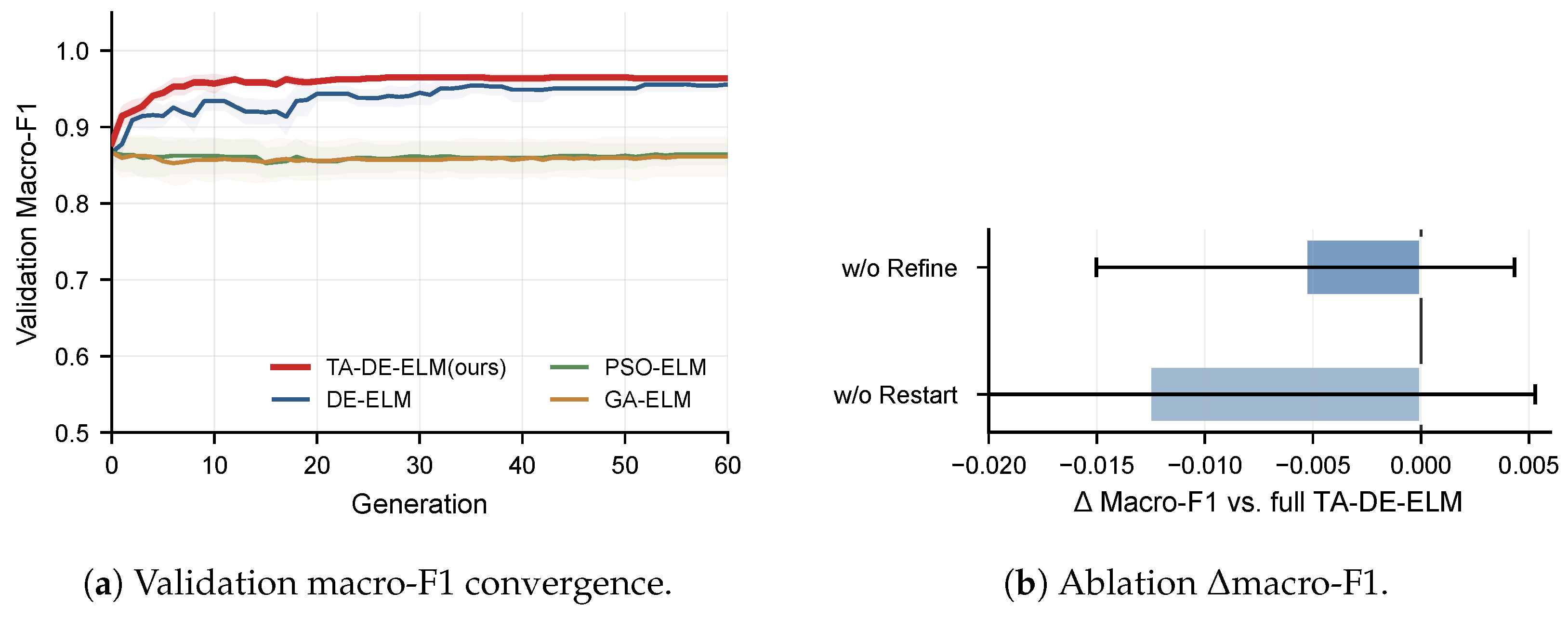
To examine optimization behavior directly, we traced the best-so-far validation macro-F1 at each generation for TA-DE-ELM, DE-ELM, PSO-ELM, and GA-ELM. Because TA-DE-ELM uses validation perturbation during its native candidate scoring, all the traced candidates were re-evaluated with a common clean validation evaluator before plotting. Figure 5 therefore reports the convergence under this shared evaluator, alongside the ablation delta.

4.5. Component Ablation Under Unified Budget

To verify the contribution of the proposed TA-DE mechanisms, we report a targeted ablation built around the finalized TA-DE-ELM configuration. The ablation compares the full model with two mechanism-removal variants: without elite refinement and without a stagnation-triggered restart. All the variants used the same ELM backbone, feature policy, split protocol, hidden size, population size, maximum generation budget, and repeated-run setting. To make the ablation directly comparable with the main comparison in Table 6,

Table 8. Ablation of the two-stage adaptive DE mechanisms under the finalized finite-budget protocol. The full-model row is identical to the TA-DE-ELM (ours) row in Table 6 for the shared metrics. ↓ indicates that lower values are better.

Variant	Accuracy	Macro-F1	QWK	Ordinal MAE ↓	$\Delta$ Macro-F1
TA-DE-ELM (ours)	$\mathbf{0.9404}\pm \mathbf{0.0084}$	$\mathbf{0.9396}\pm \mathbf{0.0084}$	$\mathbf{0.9899}\pm \mathbf{0.0014}$	$\mathbf{0.0119}\pm \mathbf{0.0017}$	$+0.0000$
w/o Refine	$0.9351\pm 0.0097$	$0.9342\pm 0.0097$	$0.9890\pm 0.0017$	$0.0130\pm 0.0019$	$-0.0053$
w/o Restart	$0.9285\pm 0.0170$	$0.9270\pm 0.0179$	$0.9879\pm 0.0029$	$0.0143\pm 0.0034$	$-0.0126$

repeats the same four held-out metrics and adds the macro-F1 change relative to the full model.

Table 8 and Figure 5b show that both mechanisms contribute under the final budget. Removing elite refinement decreases Macro-F1 by $0.0053$, while removing restart decreases the macro-F1 by $0.0126$ and increases the run-to-run variance. The restart result is particularly relevant because premature convergence is a common risk in high-dimensional ELM input-parameter searches. These ablation results support the use of a two-stage adaptive DE design rather than plain DE alone.

4.6. Confusion Matrix and Error Pattern Analysis

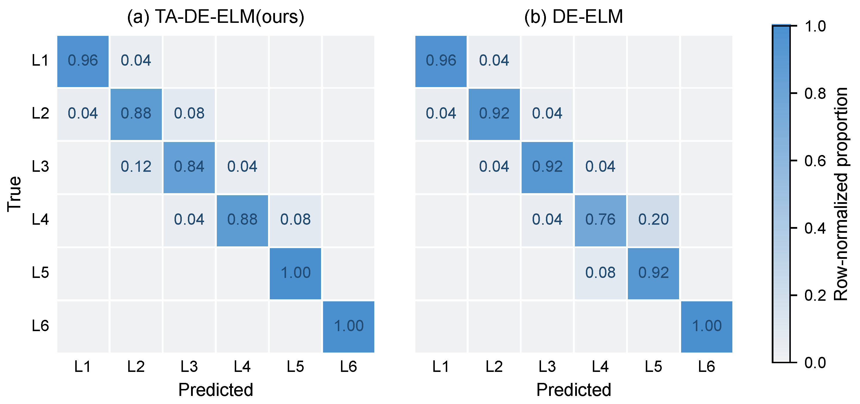
To verify the error structure, we inspected the normalized confusion matrices of TA-DE-ELM and DE-ELM on the held-out test set. Figure 6 shows that the residual errors in both models were concentrated in adjacent risk levels along the main diagonal, with no severe long-range confusions (e.g., predicting level 1 as level 6 or vice versa). TA-DE-ELM placed more mass on the diagonal across all six levels, consistent with its higher per-class F1 scores and lower ordinal MAE ($0.0119$). Across all five ELM-family models, every misclassification was an adjacent-1 error with no severe or adjacent-2+ confusion, and TA-DE-ELM achieved the lowest adjacent-1 error rate (6.0%), confirming that all residual misclassifications are boundary-proximal.

4.7. Robustness Under Feature Degradation

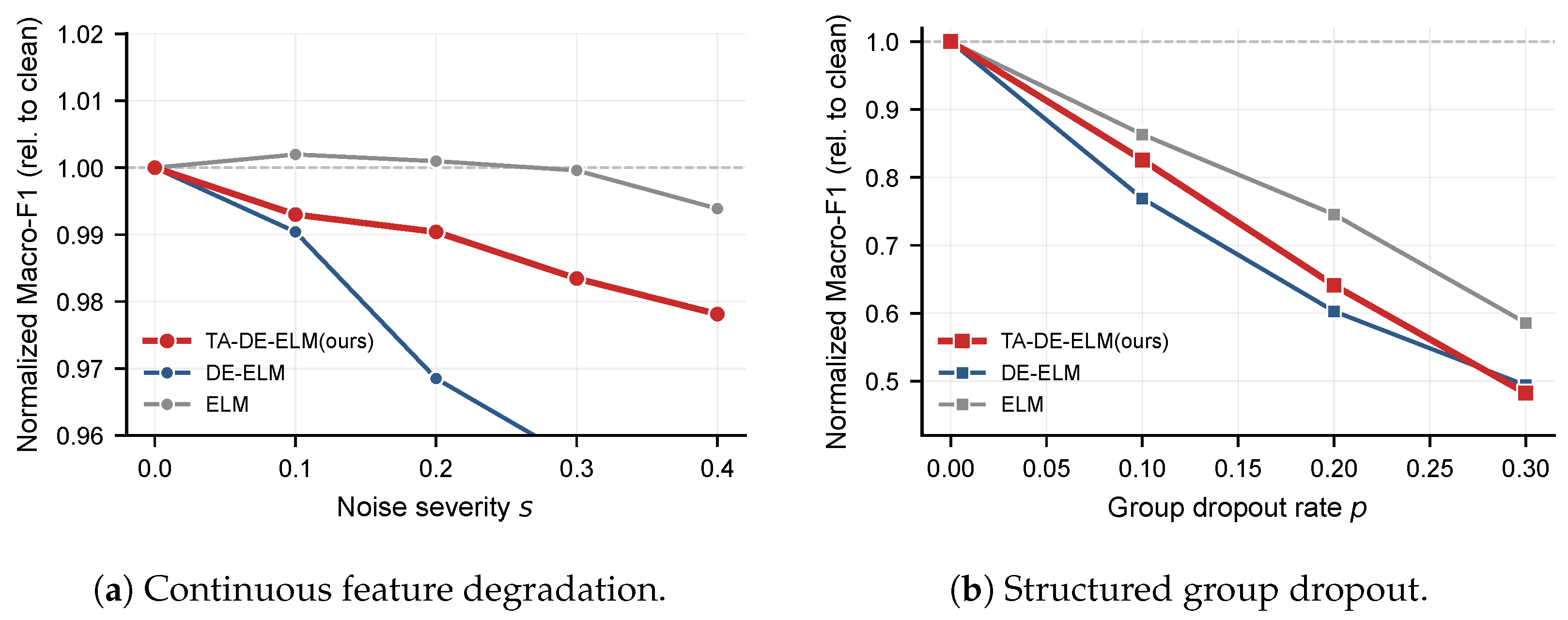
Modern sensing pipelines routinely suffer from noise contamination and structured feature dropouts. To test the degradation sensitivity, we evaluated two perturbation families on TA-DE-ELM, DE-ELM, and the standard ELM: (i) continuous feature degradation with additive Gaussian noise swept across five severity levels and (ii) structured group dropout with masking rates up to 0.3 applied to complete feature groups. Figure 7 reports the macro-F1 normalized to each model’s clean baseline, isolating the degradation rate from the baseline quality.

Under continuous noise, TA-DE-ELM exhibited the slowest relative degradation ($-2.2\%$ at $s=0.4$ vs. $-5.0\%$ for DE-ELM), indicating that its refinement mechanism does not produce brittle solutions. Under structured group dropout, all models degraded heavily at high dropout rates ($p\ge 0.2$), with the ELM showing an unexpectedly strong relative retention. This suggests that the structured nature of the perturbation—masking entire feature groups—overwhelms optimizer-level differences and is dominated by the shared ELM backbone’s ability to exploit the remaining feature groups. The noise result is consistent with improved local stability under the TA-DE search, while the dropout result is a limitation that motivates the investigation of richer perturbation families in future work.

4.8. Computational Cost

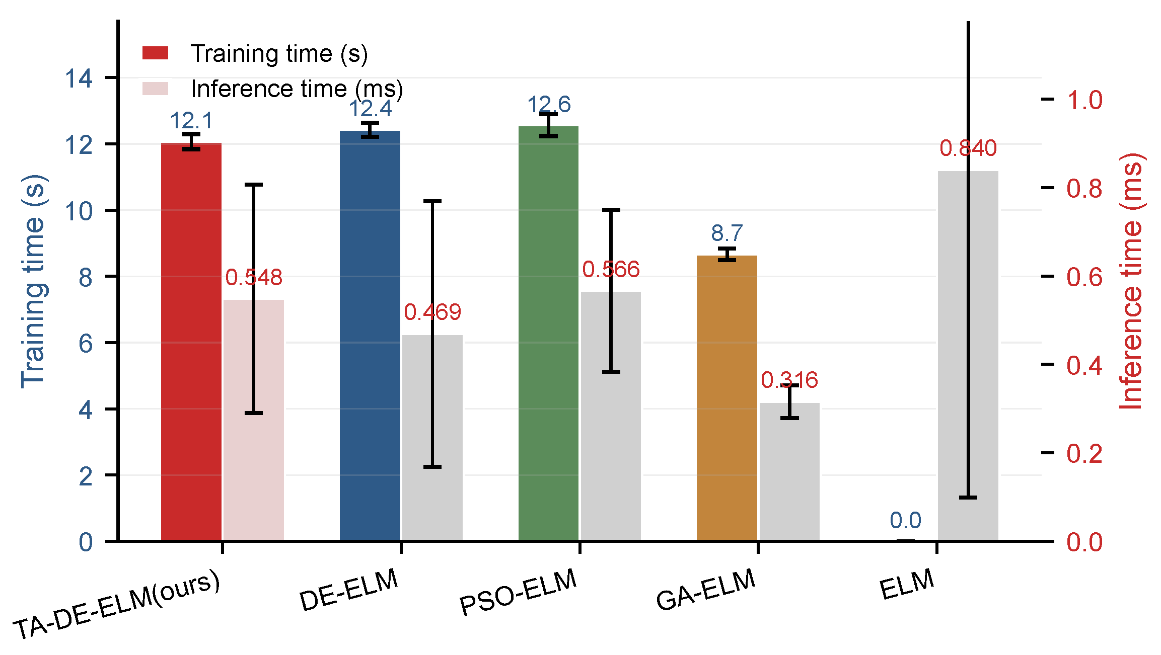
All ELM-family models used the same backbone ($H=128$) and differed only in how the input weights and biases were initialized or optimized. Figure 8 reports the measured wall-clock training and inference times under the unified finite budget ($P=24$, $T=60$). The training times were comparable across evolutionary optimizers (8.7–12.6 s), and inference latency was sub-millisecond for all variants. TA-DE-ELM achieved the best accuracy–cost trade-off without increasing the per-evaluation cost relative to DE-ELM. The additional refinement and restart operations contributed negligible overhead (<2% of total training time), indicating that the gains came from search adaptation rather than a larger computational budget.

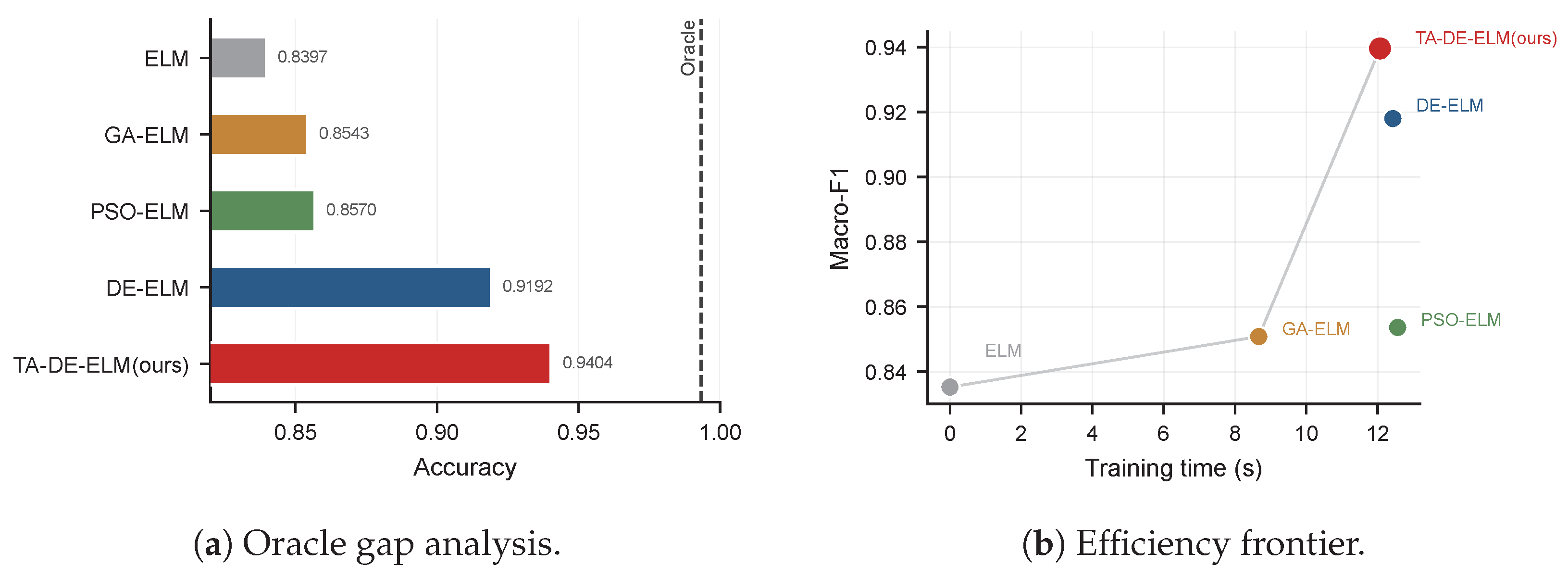
4.9. Oracle Ceiling and Efficiency Frontier

The Oracle baseline (Section 4.2) establishes that the noise-free scoring function achieved an accuracy of 0.9934 on this benchmark. Figure 9a shows how much of the Oracle-to-ELM gap each model closes. TA-DE-ELM reached 0.9404, closing 28.6% of the DE-ELM-to-Oracle gap with no additional computational budget. The efficiency frontier in Figure 9b shows that TA-DE-ELM sits on the Pareto front: no tested model achieved a higher macro-F1 at a shorter or equal training time. This jointly addresses the concern that performance gains might come from a larger budget (they do not) and that the benchmark is not equally solved by all tested learning methods.

5. Conclusions

This work presented TA-DE-ELM, a six-level ordered-risk assessment framework that combines an expert-rule-guided synthetic benchmark with two-stage adaptive differential evolution for ELM parameter optimization. The framework tests whether a lightweight nonlinear model can recover an explicit ordered-risk mapping under limited-label conditions while keeping the benchmark assumptions and evaluation budget transparent. Under the unified finite-budget protocol, TA-DE-ELM ranked first among the tested ELM-family baselines across accuracy, macro-F1, QWK, and ordinal MAE. It reached an accuracy of $0.9404$ and a macro-F1 of $0.9396$; paired-run tests indicated a macro-F1 improvement over DE-ELM, with no additional inference cost. It also exceeded traditional scoring and ranking references such as RF-GRA and Entropy-GRA. Together with the ablation study, confusion-matrix inspection, convergence trace, and Oracle-ceiling analysis, these results indicate that the two-stage adaptive design improves classification performance and risk-order consistency under budget parity.

These findings should be interpreted within the limits of the controlled benchmark. The labels are generated from fixed expert-prior weights and score edges, so the model learns a benchmark-induced ordered-risk mapping rather than validating a specific real-world decision process. The benchmark and its sensitivity analysis establish internal consistency but do not replace application-specific validation. The ELM backbone and the tested perturbation families also remain simpler than real sensing and degradation scenarios. The results therefore provide controlled feasibility evidence for early-stage model screening and methodological comparison. Future validation should use higher-fidelity simulation, external datasets, dynamic multi-entity scenarios, richer degradation protocols, and expert review.