A Combined MMSE/MMSE-IRC Receiver with Alternating Projections Successive Interference Cancellation for ICI Mitigation in 5G-NR Uplink

Abstract

The evolution from 4G Long-Term Evolution (LTE) to 5G New Radio (NR) has increased cell density in cellular deployments, thereby increasing inter-cell interference (ICI), which is most significant in cell-edge scenarios. The Minimum Mean Square Error–Interference Rejection Combining (MMSE-IRC) receiver was widely adopted in LTE systems around Release 11 as a practical implementation for advanced interference rejection. Although not standardized in 3GPP specifications, it was commonly used in 3GPP studies and has been effectively used in 5G-NR environments. In this paper, we propose new versions of the Alternating Projections Hard Successive Interference Cancellation (AP-HSIC) equalizer algorithm that combine the Minimum Mean Square Error (MMSE) and MMSE-IRC equalizers (denoted MMSE-AP-HSIC and MMSE-IRC-AP-HSIC, respectively). The effectiveness of the new approach is demonstrated by Block Error Rate (BLER) analysis for Quadrature Phase Shift Keying (QPSK), 16-QAM, and 64-QAM modulations. Physical Uplink Shared Channel (PUSCH) 5G-NR receiver simulations demonstrate the differences between the proposed algorithms and the classical AP-HSIC, MMSE, and MMSE-IRC equalizer algorithms. Simulation results show that the proposed scheme, MMSE-IRC-AP-HSIC, outperforms the conventional MMSE-IRC scheme in cell-edge scenarios.

1. Introduction

Fifth-generation New Radio (5G-NR) networks are increasingly deployed as dense, small-cell topologies, in which base stations are placed close to one another and the available frequency resources are aggressively reused. This densification raises system capacity, but it also makes inter-cell interference (ICI) the dominant impairment for cell-edge users, whose uplink transmissions reach the serving base station at low signal-to-interference-plus-noise ratio (SINR) and are corrupted by co-scheduled transmissions from neighboring cells. Mitigating ICI at the receiver of the serving base station, without requiring channel state information (CSI) to be fed back to the transmitter and without requiring the interfering signals to be explicitly decoded, is therefore a central problem for the 5G-NR uplink. The background to this problem, and the interference-mitigation approaches that have been proposed to address it, are reviewed in Section 2.

In this paper, we propose new versions of the Alternating Projections Hard Successive Interference Cancellation (AP-HSIC) equalizer algorithm [1] that combine it with the Minimum Mean Square Error (MMSE) and Minimum Mean Square Error–Interference Rejection Combining (MMSE-IRC) equalizers, denoted MMSE-AP-HSIC and MMSE-IRC-AP-HSIC, respectively. AP-HSIC is an iterative, digital successive interference cancellation (SIC) method that jointly estimates the desired symbols and the residual interference distortion by alternating projections onto two convex sets, without requiring the interferers to be explicitly decoded. The proposed algorithms are designed to draw on the complementary strengths of the three families discussed above while avoiding their main limitations. Like the SIC family, they operate entirely at the receiver and do not require physical CSI feedback to the transmitter, so they remain practical as the number of base station (BS) antennas grows and the downlink (DL) CSI strategy of beamforming-based schemes becomes infeasible. Unlike classical SIC, however, the alternating-projections mechanism does not rely on explicitly reconstructing and subtracting each interferer, which allows it to cope with external, highly correlated, and time-asynchronous interference that violates the assumptions of conventional SIC decoding. Finally, by initializing the iterations with an MMSE or MMSE-IRC estimate instead of the zero-forcing solution used in [1], the proposed MMSE-IRC-AP-HSIC variant inherits the spatial interference-rejection capability of the MMSE-IRC family and refines it through successive cancellation, yielding improved block error rate (BLER) performance in low-SINR cell-edge scenarios, as demonstrated by the simulations in this paper.

The remainder of this paper is organized as follows. Section 2 provides the background on multipath fading, Multiple-Input Multiple-Output (MIMO) transmission, cell densification, and interference in 5G-NR, and reviews the related work on interference-mitigation approaches. Section 3 presents the system and interference models, developing the per-subcarrier and compact matrix formulations of the received signal and detailing the dominant interference proportion (DIP)-based inter-cell interference model used in this study. Section 4 develops the proposed iterative SIC algorithm: it progresses from the classical MMSE and MMSE-IRC formulations to the AP-HSIC model, and describes how the AP-HSIC algorithm is integrated with the MMSE and MMSE-IRC equalizers to form the proposed MMSE-AP-HSIC and MMSE-IRC-AP-HSIC decoding chains. Section 5 details the simulation parameters and reports the Physical Uplink Shared Channel (PUSCH) link-level simulation results, comparing the proposed algorithms against the classical AP-HSIC, MMSE, and MMSE-IRC equalizers in terms of BLER versus SINR for Quadrature Phase Shift Keying (QPSK), 16-QAM, and 64-QAM, with and without ICI. Finally, Section 6 summarizes the findings and concludes the paper with emphasis on the practical comparison between 5G-NR receiver algorithms.

2. Background and Related Work

2.1. Multipath Fading, MIMO, and Interference in Densified 5G-NR Networks

Wireless communication is mainly degraded by multipath fading, which occurs when the transmitted signal reaches the receiver through different paths, angles, delays, or Doppler shifts caused by scattering in the environment. Due to angle, delay, and Doppler spreads, the received signal power randomly fluctuates over space, frequency, and time, a phenomenon known as fading, which can severely degrade wireless communication quality and reliability. Moreover, limited power and bandwidth further complicate the design of highly reliable high-rate wireless systems [2]. Exploiting multipath scattering, Multiple-Input Multiple-Output (MIMO) techniques deliver significant performance enhancements in terms of data transmission rate, and interference reduction is achieved through mechanisms that enable the creation of uncorrelated and spatially multiplexed MIMO channels with high diversity order, high spatial selectivity [3], and diversity gain.

Cellular systems in urban areas now mostly use smaller cells with base stations close to the street level and transmitting at much lower power. This evolution to smaller cells occurred for two reasons: the need for higher capacity in areas with high user equipment (UE) density and the reduced size and cost of base station (BS) electronics. However, the evolution to smaller cells has complicated network design. Mobiles traverse a small cell more quickly than a large cell, and therefore, hand-offs must be processed more quickly. In addition, location management becomes more complicated, as there are more cells within a given area where a mobile device may be located [4]. It is also more challenging to develop general propagation models for small cells, as a hexagonal layout does not accurately represent signal behavior in microcell environments. In practice, microcellular systems are commonly planned using square or triangular layouts; however, these geometries still introduce considerable approximation errors when modeling microcell propagation [5].

The NR cellular network has increased cell density in cellular deployments, thus increasing ICI, and interference mitigation techniques become more critical. Interference is most limiting when considering cell-edge users, which experience significant interference from users associated with neighboring cells. In addition to increasing cell density, a key technology that has evolved the 5G-NR generation is massive MIMO, which offers a large number of antennas at the BS and increases energy efficiency and spectral efficiency [6]. To achieve a high system performance, one must consider the fact that the knowledge of channel state information (CSI) at the BS has a key role. Under frequency division duplexing (FDD), the uplink (UL) and downlink (DL) use different frequency bands, leading to distinct CSI for each link. As the number of BS antennas increases, the traditional DL channel estimation strategy for FDD systems becomes infeasible, and the most effective and probable way of obtaining CSI is in a time division duplexing (TDD) system by incorporating reciprocity, which allows the CSI required for DL beamforming to be obtained from pilots in the UL transmission process, so only the CSI for the UL needs to be estimated [7].

Unlike LTE-TDD, which requires the UL/DL sub-frame configurations of all cells using the same frequency band to be synchronized, called Static TDD (S-TDD), 5G NR supports dynamic TDD (D-TDD) as a way of improving performance by obtaining duplexing flexibility that adaptively schedules UL and DL traffic according to the traffic conditions. The advantages of the D-TDD system are difficult to fully utilize due to cross-link interference (CLI) arising from the use of different transmission directions between adjacent cells that causes asynchronous ICI [8]. For UL D-TDD, in addition to UE-to-BS interference, the BS receives interference from the BSs in the adjacent DL cells, called BS-to-BS interference, which degrades the UL signal-to-interference-plus-noise ratio (SINR) performance in D-TDD systems compared to S-TDD systems because the interference power of a BS transmitted in an adjacent cell is usually higher than that of UEs in adjacent cells [9]. In addition, in multiple cells, where each cell is enclosed with tens of antennas that evolve into a massive MIMO system, to achieve high system performance, the provision of pilot signals to users happens to be the main obstacle, and the allocation of distinct orthogonal pilot signals to users in each cell is not considered feasible due to bandwidth limitations [10].

2.2. Related Work on Interference-Mitigation Approaches

Several approaches have been developed in recent years to address the challenges of offsetting the destructive effects of various interference sources in general and ICI in particular. The main approaches can be classified as follows: successive interference cancellation (SIC) approaches [11,12,13,14], MMSE-IRC [15], and advanced MIMO-beamforming techniques such as the analog–digital hybrid-beamforming structure [16,17] and multilayer precoding like [18,19]. The first family has algorithms such as classical SIC [11,12] and SIC based on machine learning/deep learning algorithms such as SICnet [13] and DeepSIC [14]. The main benefit of these techniques is that they do not require physical CSI feedback from the receiver to the transmitter. However, they struggle to handle interference from external sources, such as nearby users whose signals are highly correlated with the desired transmission or an active intelligent jammer in the same spatial region. This limitation arises because such external disturbances violate the assumption of the internal offset process used in the SIC algorithm, disrupting the iterative decoding and significantly degrading system performance.

The second family is based on the MMSE-IRC equalizer [15]. The MMSE-IRC provides spatial selectivity, handles interference from neighboring users within the network framework, offers high diversity, and supports advanced spatial multiplexing. However, it is limited in mitigating dynamic external interference and destructive wireless effects, as its design relies heavily on non-stand-alone (NSA) networks and network-based protocols using PUSCH and the Demodulation Reference Signal (DMRS). The third family is beamforming techniques: hybrid beamforming such as [16,17], analog–digital beamforming, and multilayer precoding systems like [18,19]. The disadvantage of this approach is that the receiver must share the DL CSI via physical feedback. As mentioned above, as the number of BS antennas becomes large, the DL CSI strategy for FDD systems becomes infeasible. Even in advanced TDD systems such as D-TDD, there are challenges in DL CSI collaboration, like BS-to-BS interference and CLI that cause asynchronous ICI, which has a strong impact on the null-steering capabilities of the receiver and the respective interference mitigation performance [20].

3. System and Interference Model

In this section, we present the system and interference models adopted in the paper.

3.1. System Model

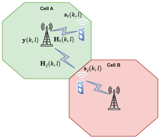
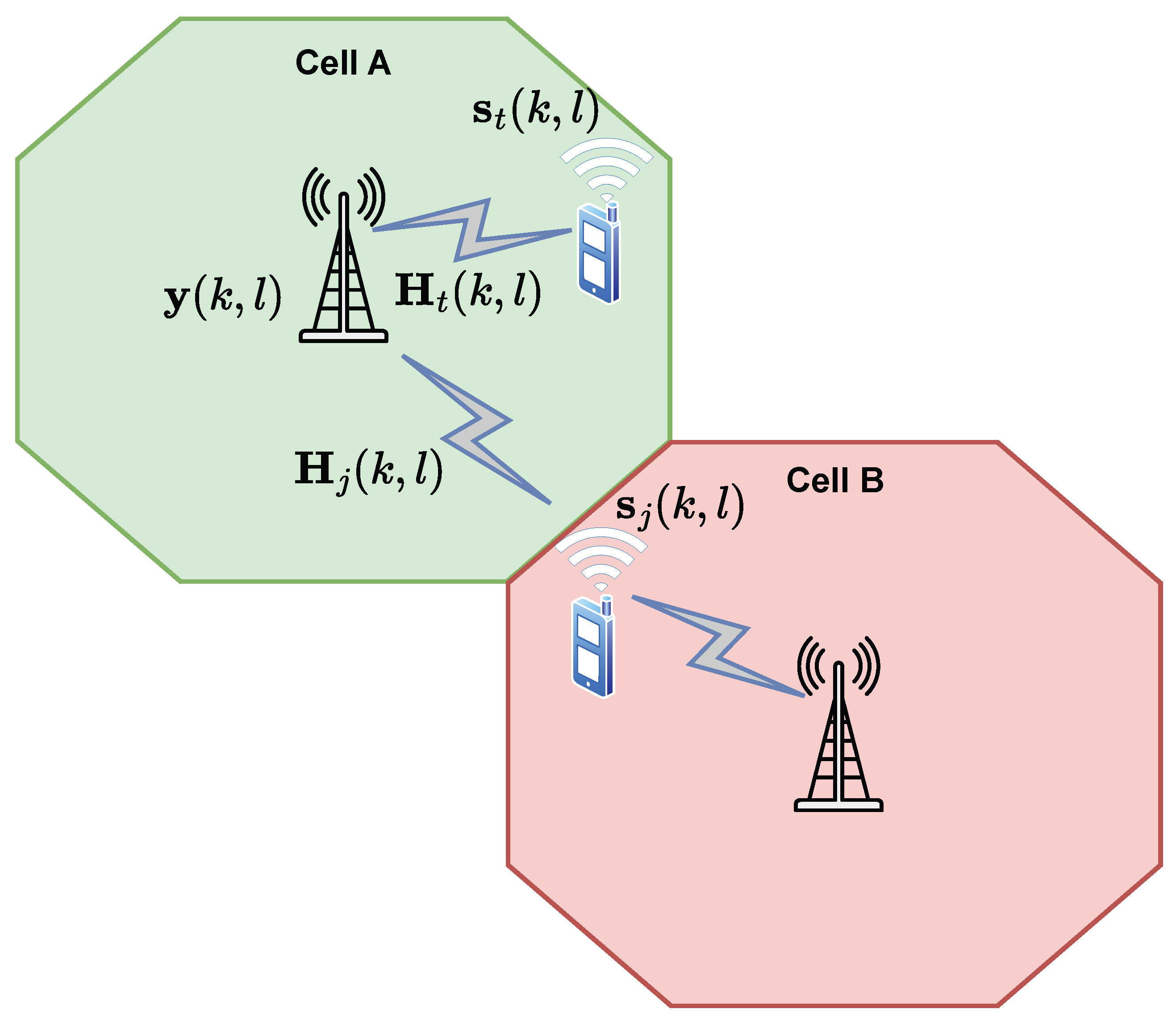
In this classical communication scenario, we examine two 5G-NR BSs that create two adjacent spatial cells. In cell A, the desired UE is located and is transmitting on the uplink channels to its serving 5G-NR BS. In cell B, several UEs are present, causing interference to the serving 5G-NR BS in cell A (see Figure 1). The uplink transmission is modeled as an MIMO system with multiple transmit and receive antennas. Throughout, $k=0,\dots ,K-1$ denotes the subcarrier index and $\ell =0,\dots ,L-1$ the Fast Fourier Transform Orthogonal Frequency Division Multiplexing (FFT-OFDM) symbol index, where K and L are the total numbers of subcarriers and FFT-OFDM symbols, respectively. The desired UE’s transmitted symbol vector is ${\mathbf{s}}_t\left(k,\ell \right)$, with dimension $N_{TX}\times 1$. Its channel to the BS is ${\mathbf{H}}_t\left(k,\ell \right)$, an $N_{RX}\times N_{TX}$ frequency-selective Rayleigh fading matrix. For each interferer j, the transmitted symbol vector is ${\mathbf{s}}_j\left(k,\ell \right)$, of dimension $N_{TX}^{\left(j\right)}\times 1$, and the corresponding channel is ${\mathbf{H}}_j\left(k,\ell \right)$, of size $N_{RX}\times N_{TX}^{\left(j\right)}$. The thermal noise vector $\mathbf{n}\left(k,\ell \right)$ is $N_{RX}\times 1$ additive white Gaussian noise (AWGN). The received signal is then represented by $\mathbf{y}\left(k,\ell \right)$, which is the $N_{RX}\times 1$ receive vector at the serving BS. Here, j indexes the interferers and J is the total number of interferers.

Figure 1. Uplink ICI scenario illustrating the considered system model. The desired UE is located in Cell A and communicates with its serving BS. An interfering UE is located in the neighboring Cell B.

The received signal is then given by [21]:

$$\mathbf{y}\left(k,\ell \right)={\mathbf{H}}_t\left(k,\ell \right){\mathbf{s}}_t\left(k,\ell \right)+\sum _j{\mathbf{H}}_j\left(k,\ell \right){\mathbf{s}}_j\left(k,\ell \right)+\mathbf{n}\left(k,\ell \right),$$

(1)

Table 1 summarizes the per-subcarrier variables and their dimensions.

Table 1. Per-subcarrier variables and dimensions in the scalar system model.

Symbol	Description	Dimensions
${\mathbf{s}}_t\left(k,\ell \right)\phantom{N_{TX}^{\left(j\right)}}$	Desired UE transmitted symbol vector	$N_{TX}\times 1\phantom{N_{TX}^{\left(j\right)}}$
${\mathbf{H}}_t\left(k,\ell \right)\phantom{N_{TX}^{\left(j\right)}}$	Desired UE channel matrix	$N_{RX}\times N_{TX}\phantom{N_{TX}^{\left(j\right)}}$
${\mathbf{s}}_j\left(k,\ell \right)\phantom{N_{TX}^{\left(j\right)}}$	Interferer-j transmitted symbol vector	$N_{TX}^{\left(j\right)}\times 1\phantom{N_{TX}^{\left(j\right)}}$
${\mathbf{H}}_j\left(k,\ell \right)\phantom{N_{TX}^{\left(j\right)}}$	Channel matrix of interferer j	$N_{RX}\times N_{TX}^{\left(j\right)}\phantom{N_{TX}^{\left(j\right)}}$
$\mathbf{n}\left(k,\ell \right)\phantom{N_{TX}^{\left(j\right)}}$	AWGN vector	$N_{RX}\times 1\phantom{N_{TX}^{\left(j\right)}}$
$\mathbf{y}\left(k,\ell \right)\phantom{N_{TX}^{\left(j\right)}}$	Received signal vector at BS	$N_{RX}\times 1\phantom{N_{TX}^{\left(j\right)}}$

For each resource block (RB) in a particular FFT-OFDM symbol ℓ, it is possible to switch from (1) to a matrix representation. The channel is frequency-selective across the carrier, so that each RB carries its own channel matrix and the equalization is performed independently per RB, but it is taken to be constant over the K subcarriers of a single RB, which span 360 kHz at the 30 kHz subcarrier spacing used here. It is this block-fading assumption at RB granularity that allows the per-subcarrier matrices ${\mathbf{H}}_t\left(k,\ell \right)$ and ${\mathbf{H}}_j\left(k,\ell \right)$ to be replaced by the single matrices ${\mathbf{H}}_T$ and ${\mathbf{H}}_j$ in what follows. Retaining the variation of the channel within a single RB would require a block-diagonal formulation, which is beyond the scope of the present work. Let

$$\begin{array}{cc}\hfill \mathbf{Y}& =\left[\begin{array}{ccc}\mathbf{y}\left(0\right)& \cdots & \mathbf{y}\left(K-1\right)\end{array}\right],\hfill \\ \hfill \mathbf{N}& =\left[\begin{array}{ccc}\mathbf{n}\left(0\right)& \cdots & \mathbf{n}\left(K-1\right)\end{array}\right],\hfill \\ \hfill \mathbf{S}& =\left[\begin{array}{ccc}{\mathbf{s}}_t\left(0\right)& \cdots & {\mathbf{s}}_t\left(K-1\right)\end{array}\right],\hfill \\ \hfill {\mathbf{S}}_j& =\left[\begin{array}{ccc}{\mathbf{s}}_j\left(0\right)& \cdots & {\mathbf{s}}_j\left(K-1\right)\end{array}\right],.\hfill \end{array}$$

(2)

Then,

$$\mathbf{Y}={\mathbf{H}}_T\mathbf{S}+\sum _j{\mathbf{H}}_j{\mathbf{S}}_j+\mathbf{N}.$$

(3)

where $\mathbf{Y}$ and $\mathbf{N}$, of size $N_{RX}\times K$, collect the received signal and noise across the K subcarriers of the resource block; $\mathbf{S}$ and ${\mathbf{S}}_j$, of sizes $N_{TX}\times K$ and $N_{TX}^{\left(j\right)}\times K$, are the desired and interfering transmitted symbols; and ${\mathbf{H}}_T$ and ${\mathbf{H}}_j$, of sizes $N_{RX}\times N_{TX}$ and $N_{RX}\times N_{TX}^{\left(j\right)}$, are the corresponding channel matrices, where $N_{TX}$ and $N_{TX}^{\left(j\right)}$ are the numbers of transmitted streams of the desired UE and the j-th interferer, respectively.

Let

$$\begin{array}{cc}\hfill & {\mathcal{H}}_J=\left[\begin{array}{ccc}{\mathbf{H}}_1& \cdots & {\mathbf{H}}_J\end{array}\right],\hfill \\ \hfill & {\mathcal{S}}_J=\left[\begin{array}{c}{\mathbf{S}}_1\\ ⋮\\ {\mathbf{S}}_J\end{array}\right],\hfill \end{array}$$

(4)

The calligraphic symbols ${\mathcal{H}}_J$ and ${\mathcal{S}}_J$ denote the aggregate interference channel and symbol matrices, obtained by stacking the contributions of all J interferers; the subscript J therefore refers to the complete set of interferers, and not to any single one of them. This is to be distinguished from the boldface ${\mathbf{H}}_j$ and ${\mathbf{S}}_j$, $j=1,\dots ,J$, which denote the channel and symbol matrices of the individual j-th interferer, as defined above. The aggregate matrices ${\mathcal{H}}_J$ and ${\mathcal{S}}_J$ are of sizes $N_{RX}\times \left({\sum }_{j=1}^J{N}_{TX}^{\left(j\right)}\right)$ and $\left({\sum }_{j=1}^J{N}_{TX}^{\left(j\right)}\right)\times K$, respectively. The notation ${\mathcal{H}}_J$, ${\mathcal{S}}_J$ introduced in (4) is used consistently throughout the remainder of the paper. The interference model is given by

$$\mathbf{Y}={\mathbf{H}}_T\mathbf{S}+{\mathcal{H}}_J{\mathcal{S}}_J+\mathbf{N},$$

(5)

where $\mathbf{Y}$ and ${\mathbf{H}}_T$ are assumed to be known, but $\mathbf{S}$, ${\mathcal{H}}_J$, and ${\mathcal{S}}_J$ are unknowns.

Table 2 summarizes the matrix-form variables and their dimensions.

Table 2. Compact matrix-form variables and dimensions.

Symbol	Description	Dimensions
$\mathbf{Y}\phantom{N_{TX}^{\left(j\right)}}$	Received signal matrix across K subcarriers	$N_{RX}\times K\phantom{N_{TX}^{\left(j\right)}}$
$\mathbf{N}\phantom{N_{TX}^{\left(j\right)}}$	Noise matrix across K subcarriers	$N_{RX}\times K\phantom{N_{TX}^{\left(j\right)}}$
$\mathbf{S}\phantom{N_{TX}^{\left(j\right)}}$	Desired UE transmit symbol matrix	$N_{TX}\times K\phantom{N_{TX}^{\left(j\right)}}$
${\mathbf{S}}_j\phantom{N_{TX}^{\left(j\right)}}$	Interferer-j transmit symbol matrix	$N_{TX}^{\left(j\right)}\times K\phantom{N_{TX}^{\left(j\right)}}$
${\mathbf{H}}_T\phantom{N_{TX}^{\left(j\right)}}$	Desired UE channel matrix	$N_{RX}\times N_{TX}\phantom{N_{TX}^{\left(j\right)}}$
${\mathbf{H}}_j\phantom{N_{TX}^{\left(j\right)}}$	Interferer-j channel matrix (boldface, single interferer)	$N_{RX}\times N_{TX}^{\left(j\right)}\phantom{N_{TX}^{\left(j\right)}}$
${\mathcal{H}}_J$	Aggregated channel matrix of all J interferers (calligraphic); see (4)	$N_{RX}\times \left({\sum }_{j=1}^J{N}_{TX}^{\left(j\right)}\right)$
${\mathcal{S}}_J$	Aggregated symbol matrix of all J interferers (calligraphic); see (4)	$\left({\sum }_{j=1}^J{N}_{TX}^{\left(j\right)}\right)\times K$

3.2. Interference Model

There is no known description of the interference model in the 5G-NR specification, so the 4G one was used, as in [22] Section 8.2.6 and Annex B.6. The inter-cell interference is set to be time-synchronous or time-asynchronous, whereby in each slot, each interferer transmits 16-QAM randomly modulated data over the entire PUSCH region and the same resource blocks as the tested signal. Each interferer has unique PUSCH data bits, which is ensured by providing a unique pseudo-random sequence seed. The DMRS reference symbols were modeled to be unique to each interferer (and to the UE) by setting a unique DMRS scrambling ID ($N_{ID}^{{\overline{n}}_{SCID}^{\overline{\lambda }}}$ in [23] section 6.4.1.1.1.1). Finally, each interferer is assumed to have the same multipath delay spread and Doppler as the UE, but a unique channel seed is set.

Each interferer is characterized by its associated dominant interference proportion (DIP) value, defined as in [22] Annex B.6:

$${\mathrm{DIP}}_j={\displaystyle \frac{{\overline{I}}_j}{{\sigma }_n^2+{\sum }_j{\overline{I}}_j}},$$

(6)

where ${\overline{I}}_j$ is the average power received at the receive antenna port from the j-th inter-cell interferer, J is the number of interferers, and ${\sigma }_n^2+{\sum }_j{\overline{I}}_j$ is the total noise-plus-interference power at the port, where ${\sigma }_n^2$ is the power of the AWGN. The DIP is convenient because it allows the SINR at the receive antenna port to be expressed directly in terms of the DIP and the signal-to-noise ratio (SNR), as shown in (8). To this end, the SNR at the receive antenna port is first defined as follows:

$$\mathrm{SNR}={\displaystyle \frac{{\overline{P}}_s}{{\sigma }_n^2}}.$$

(7)

where ${\overline{P}}_s$ is the power of the desired signal.

Using the DIP and the SNR, the SINR at the receive antenna port is given by

$$\mathrm{SINR}={\displaystyle \frac{{\overline{P}}_s}{{\sigma }_n^2+{\sum }_j{\overline{I}}_j}}={\displaystyle \frac{{\overline{P}}_s}{{\sigma }_n^2}}\left(1-{\displaystyle \frac{{\sum }_j{\overline{I}}_j}{{\sigma }_n^2+{\sum }_j{\overline{I}}_j}}\right)=\mathrm{SNR}\left(1-\sum _j{\mathrm{DIP}}_j\right),$$

(8)

Two sets of DIP values for up to two interferers are given in [22] section 8.2.6:

$$\begin{array}{cccc}\hfill \mathrm{DIP} \mathrm{set} 1: & \left[-1.11,-10.91\right]\mathrm{dB}\hfill & \hfill & \equiv \left[0.7745,0.0811\right],\hfill \\ \hfill \mathrm{DIP} \mathrm{set} 2: & \left[-0.43,-13.78\right]\mathrm{dB}\hfill & \hfill & \equiv \left[0.9057,0.0419\right].\hfill \end{array}$$

(9)

where the quantities on the left are expressed in dB and those on the right are the corresponding linear power ratios, obtained as ${\mathrm{DIP}}_j={10}^{{\mathrm{DIP}}_j\left[\mathrm{dB}\right]/10}$. The linear form is given explicitly because it makes the physical constraint on the DIP immediately visible: summing the entries of each set yields ${\sum }_j{\mathrm{DIP}}_j=0.8556$ for set 1 and ${\sum }_j{\mathrm{DIP}}_j=0.9476$ for set 2, both of which are strictly smaller than unity. This is required by the definition in (6), as ${\sum }_j{\mathrm{DIP}}_j=\left({\sum }_j{\overline{I}}_j\right)/\left({\sigma }_n^2+{\sum }_j{\overline{I}}_j\right)=1-{\sigma }_n^2/\left({\sigma }_n^2+{\sum }_j{\overline{I}}_j\right)<1$ for any ${\sigma }_n^2>0$. The residual $1-{\sum }_j{\mathrm{DIP}}_j$ is therefore precisely the fraction of the total interference-plus-noise power that is contributed by the thermal noise, namely, $0.1444$ for set 1 and $0.0524$ for set 2. Set 2 consequently describes the more severe interference environment, with $94.8\%$ of the total impairment power originating from the two interferers as against $85.6\%$ for set 1, and it is the set adopted for the ICI simulations reported in Section 5.

The use of a quantity defined for LTE in a 5G-NR study warrants a brief justification. What is imported from [22] is the DIP, which, by the definition in (6), is a ratio of average received powers at the receive antenna port. It is therefore a dimensionless power-partition parameter: it specifies how the total impairment power at the port is divided between the dominant neighboring cells and the thermal noise floor, and it contains no subcarrier spacing, symbol duration, or cyclic-prefix length.

In this paper, we consider synchronized and non-synchronized interferers with the desired UE, similar to a neighboring heterogeneous network (HetNet) deployment [24].

To explain the phenomena of synchronized and non-synchronized interference, we first need to define several key parameters. We define ${\delta }_i$ as the spread of the time delay of the i-th path between the interfering UE and the 5G-NR service BS. In the case where the interference source is not synchronized, some (or all) of the delays of the interference paths, ${\delta }_i$, are outside the interval $\left[0,T_{CP}\right]$, where $T_{CP}$ is the duration of the cyclic prefix (CP) of the OFDM symbol at the receiver. We divide the paths into a group $\mathbb{A}$ of synchronized paths:

$$\mathbb{A}=\left\{i:{\delta }_i\in \left[0,T_{CP}\right]\right\},$$

(10)

and a complementary group $\overline{\mathbb{A}}$ of non-synchronized paths:

$$\overline{\mathbb{A}}=\left\{i:{\delta }_i\notin \left[0,T_{CP}\right]\right\}.$$

(11)

The equalizer treats the two groups identically, and requires no knowledge of which paths belong to which. Paths in $\overline{\mathbb{A}}$ violate the circular-convolution property of the CP-OFDM waveform and therefore do not reduce to a per-subcarrier multiplicative channel. They appear instead as inter-symbol and inter-carrier leakage that is neither diagonal in frequency nor confined to the subcarriers occupied by the interferer. In the model developed in Section 4, all such contributions, together with those of the synchronized paths in $\mathbb{A}$, are absorbed into the single effective channel perturbation $\Delta \mathbf{H}$, which is estimated by alternating projections rather than reconstructed from the interfering signals. No knowledge of ${\delta }_i$, of the CP alignment of the interferers, or of their channels is therefore required at the receiver, and no per-path classification is performed. The groups $\mathbb{A}$ and $\overline{\mathbb{A}}$ serve only to define the two interference conditions simulated in Section 5.

4. Proposed Iterative SIC Algorithm

In this section, we outline the development steps of the communication model, progressing from the traditional MMSE and MMSE-IRC models to the AP-HSIC model. Understanding these steps is crucial for grasping how the AP-HSIC algorithm is integrated into the decoding mechanism of the reception architecture in the 5G-NR network. Additionally, we discuss how the AP-HSIC algorithm can be combined with the MMSE and MMSE-IRC algorithms to create a serial decoding chain that enhances interference cancellation performance, which we detail later in this section. Understanding the stages of model development enhances the comprehension of the performance comparison between the algorithms, which we present later. The integration of the AP-HSIC with the MMSE and MMSE-IRC led to improvement in receiver performance in a low-SINR environment. We then compare the performance of this algorithm against the classical MMSE and MMSE-IRC algorithms in terms of BLER relative to the SINR.

4.1. AP-HSIC Model Development for 5G-NR Receiver Structure

Based on the interference model in (5), the problem at the receiver is to recover the best approximation for the desired symbol matrix $\mathbf{S}$ by solving

$$min{∥\mathbf{Y}-{\mathbf{H}}_T\mathbf{S}-{\mathcal{H}}_J{\mathcal{S}}_J∥}_F$$

(12)

where ${\mathcal{H}}_J$ and ${\mathcal{S}}_J$ are the aggregate interference channel and symbol matrices defined in (4), and $\mathbf{S}$ is constrained to be in the related M-QAM set.

The derivation that follows is built on the Moore–Penrose pseudoinverse ${\mathbf{S}}^{+}$ of the $N_{TX}\times K$ symbol matrix $\mathbf{S}$, and we therefore state the associated rank condition explicitly. Throughout this section, $\mathbf{S}$ is assumed to have full row rank, $\mathrm{rank}\left(\mathbf{S}\right)=N_{TX}$, which requires $N_{TX}\le K$.

The AP-HSIC method is as follows. Starting from model (5), multiplying from the right by ${\mathbf{S}}^{+}\mathbf{S}$ yields

$$\mathbf{Y}{\mathbf{S}}^{+}\mathbf{S}=\left({\mathbf{H}}_T+{\mathcal{H}}_J{\mathcal{S}}_J{\mathbf{S}}^{+}\right)\mathbf{S}+\mathbf{N}{\mathbf{S}}^{+}\mathbf{S}=\left({\mathbf{H}}_T+\Delta \mathbf{H}\right)\mathbf{S}+\tilde{\mathbf{N}},$$

(13)

where $\Delta \mathbf{H}={\mathcal{H}}_J{\mathcal{S}}_J{\mathbf{S}}^{+}$, with ${\mathcal{H}}_J$ and ${\mathcal{S}}_J$ as defined in (4), and $\tilde{\mathbf{N}}=\mathbf{N}{\mathbf{S}}^{+}\mathbf{S}$.

The dimensional part of the condition, $N_{TX}\le K$, is structurally satisfied in 5G-NR PUSCH and cannot be violated by any valid scheduling decision. The smallest possible frequency-domain allocation is a single physical resource block, i.e., $N_{sc}^{RB}=12$ subcarriers [23], so that $K\ge 12$, while PUSCH supports at most four spatial layers, i.e., $N_{TX}\le 4$. The new model is thus given by

$$\mathbf{Y}{\mathbf{S}}^{+}\mathbf{S}=\left({\mathbf{H}}_T+\Delta \mathbf{H}\right)\mathbf{S}+\tilde{\mathbf{N}},$$

(14)

with a related estimation problem:

$${∥\mathbf{Y}{\mathbf{S}}^{+}\mathbf{S}-\left({\mathbf{H}}_T+\Delta \mathbf{H}\right)\mathbf{S}∥}_F<ϵ.$$

(15)

However, because in the decoding process the unknown ${\mathbf{S}}^{+}\mathbf{S}$ multiplies the received signal, the algorithm is instead formulated in terms of the unprojected received matrix:

$$\mathbf{Y}=\left({\mathbf{H}}_T+\Delta \mathbf{H}\right)\mathbf{S}+\tilde{\mathbf{N}},$$

(16)

which serves as the model for the AP-HSIC algorithm. This substitution is not an uncontrolled approximation: as shown immediately below, solving the unprojected problem to the tightened threshold $ϵ/\sqrt{K}$ is a sufficient condition for the criterion stated above in terms of $\mathbf{Y}{\mathbf{S}}^{+}\mathbf{S}$ to be satisfied, so no error is incurred in the sense of that criterion. The simple and profound idea behind the AP-HSIC is the following. It is sufficient to solve, for unknowns $\mathbf{S}$ and $\Delta \mathbf{H}$ and a given $ϵ>0$, the following problem:

$$\begin{array}{cc}{∥\mathbf{Y}{\mathbf{S}}^{+}\mathbf{S}-\left({\mathbf{H}}_T+\Delta \mathbf{H}\right)\mathbf{S}∥}_F& ={∥\left(\mathbf{Y}-\left({\mathbf{H}}_T+\Delta \mathbf{H}\right)\mathbf{S}\right){\mathbf{S}}^{+}\mathbf{S}∥}_F\hfill \\ & \le {∥\mathbf{Y}-\left({\mathbf{H}}_T+\Delta \mathbf{H}\right)\mathbf{S}∥}_F{∥{\mathbf{S}}^{+}\mathbf{S}∥}_F\hfill \\ & <ϵ.\hfill \end{array}$$

(17)

Here, the first equality uses the pseudoinverse identity $\mathbf{S}{\mathbf{S}}^{+}\mathbf{S}=\mathbf{S}$, so that right-multiplying $\left({\mathbf{H}}_T+\Delta \mathbf{H}\right)\mathbf{S}$ by ${\mathbf{S}}^{+}\mathbf{S}$ leaves it unchanged and the common factor ${\mathbf{S}}^{+}\mathbf{S}$ can be pulled out on the right, while the inequality follows from the sub-multiplicativity of the Frobenius norm, ${∥\mathbf{A}\mathbf{B}∥}_F\le {∥\mathbf{A}∥}_F{∥\mathbf{B}∥}_F$.

As ${\mathbf{S}}^{+}\mathbf{S}$ is Hermitian with $0,1$ eigenvalues, it follows that

$${∥{\mathbf{S}}^{+}\mathbf{S}∥}_F\le \sqrt{K}.$$

(18)

More precisely, ${\mathbf{S}}^{+}\mathbf{S}$ is an orthogonal projector of rank $\mathrm{rank}\left(\mathbf{S}\right)$, so that ${∥{\mathbf{S}}^{+}\mathbf{S}∥}_F=\sqrt{\mathrm{rank}\left(\mathbf{S}\right)}\le \sqrt{min\left(N_{TX},K\right)}$, which under the rank condition stated above equals $\sqrt{N_{TX}}$. The bound (18) is retained in the conservative form $\sqrt{K}$ because it is valid irrespective of the rank of $\mathbf{S}$; substituting the tighter constant $\sqrt{N_{TX}}$ would only relax the threshold in the sufficient condition below. Therefore, finding $\mathbf{S}$ and $\Delta \mathbf{H}$ for which

$${∥\mathbf{Y}-\left({\mathbf{H}}_T+\Delta \mathbf{H}\right)\mathbf{S}∥}_F<{\displaystyle \frac{ϵ}{\sqrt{K}}},$$

(19)

yields the needed solution. The last problem is non-convex because ${\mathbf{H}}_T$ and $\Delta \mathbf{H}$ are multiplied unknowns. However, AP-HSIC finds approximations to these by identifying a convex envelope for the set of plausible solutions as an intersection between two convex sets. The algorithm alternates between these two convex sets until convergence is achieved. For the exact definitions of the convex sets with their related orthogonal projections, and for the proof of convergence and time-complexity, see [1]. For the distribution of $\tilde{\mathbf{N}}=\mathbf{N}{\mathbf{S}}^{+}\mathbf{S}$, and how the multiplication by ${\mathbf{S}}^{+}\mathbf{S}$ actually helps in coping with the noise part by taking a sufficiently large number of sub-carriers K, see [1].

4.2. Description of the Decoding Chain and Integrated Interference Cancellation System

In the second step, the AP-HSIC algorithm [1] is serially integrated with the MMSE and MMSE-IRC equalizers, and the performance of the combined algorithms is evaluated by analyzing the BLER as a function of the SINR. The integration forms a serial interference-cancellation decoding chain. Specifically, instead of initializing $\mathbf{S}$ with a zero-forcing (ZF) equalizer, as in [1], i.e., as ${\mathbf{H}}_T^{+}\mathbf{Y}$, we replaced the equalizer at this stage with MMSE and MMSE-IRC estimators. We refer to the resulting variants as MMSE-AP-HSIC and MMSE-IRC-AP-HSIC, respectively.

This substitution is not merely a change in starting point. The problem being solved is non-convex, and the alternating projections converge to the point of the intersection of the two convex sets that lies closest to the initial point [1]. The initializer therefore selects which solution the iteration reaches, and not only how quickly it is reached, so that starting from an MMSE-IRC estimate, whose construction accounts for the interference-plus-noise covariance, leads to a different fixed point from the zero-forcing initialization used in [1]. The two stages are, moreover, complementary rather than interchangeable: a linear equalizer cannot exploit the finite-alphabet structure of $\mathbf{S}$ and is bounded by whatever its covariance model fails to capture, while the alternating-projections stage operates on the residual that the linear stage leaves behind, absorbing it into $\Delta \mathbf{H}$ while constraining the symbol estimate to the M-QAM set.

The complexity of the alternating-projections iterations was established in [1]. A single iteration costs $O\left(max{\left(N_{RX},N_{TX},K\right)}^3\right)$, owing to the matrix products, inversions, and pseudo-inversions it performs, and the number of iterations needed to reach a tolerance $ϵ$ is $t_f=O\left(\left|ln\left(ϵ/{ϵ}_0\right)\right|\right)$, by virtue of the linear rate of convergence of alternating projections, so that the overall cost is $O\left(max{\left(N_{RX},N_{TX},K\right)}^3\left|ln\left(ϵ/{ϵ}_0\right)\right|\right)$. Here, ${ϵ}_0$ denotes the initial error, defined in [1] as the root-mean-square distance, in the joint variables $\left(\mathbf{S},\Delta \mathbf{H}\right)$, between the starting point of the iteration and the solution to which it converges. As noted in [1], the antenna and allocation dimensions are bounded in practice, so the cubic term enters as a constant multiplicative factor and the cost is governed by the iteration count.

It is worth observing that ${ϵ}_0$ is precisely the quantity that the initialization controls. An initial estimate closer to the solution reduces ${ϵ}_0$, and hence the iteration count, in addition to selecting a different point of the intersection in the manner described above, so the two effects of replacing the zero-forcing initialization act in the same direction.

For the receivers considered here this may be made concrete in terms of leading-order complex multiplications. Per resource block and per FFT-OFDM symbol, the MMSE equalizer requires $O\left(K\left(N_{RX}{N}_{TX}^2+N_{TX}^3\right)\right)$ operations, accounted for by the Gram matrix, its inversion, and its application to the received vector, and MMSE-IRC adds the estimation and inversion of the $N_{RX}\times N_{RX}$ interference-plus-noise covariance, $O\left(N_{RX}^3\right)$ per averaging group, together with the whitening, $O\left(K{N}_{RX}^2{N}_{TX}\right)$. Evaluating the pseudoinverse in the form ${\mathbf{S}}^{+}={\mathbf{S}}^H{\left(\mathbf{S}{\mathbf{S}}^H\right)}^{-1}$, which is available under the full-row-rank condition stated above and inverts an $N_{TX}\times N_{TX}$ matrix rather than a $K\times K$ one, each alternating-projections iteration costs $O\left(N_{TX}^{2}K+N_{RX}{N}_{TX}K+N_{TX}^3\right)$, the projection onto the M-QAM set requiring only comparisons. A single iteration is therefore of the same order as one linear-equalizer pass over the resource block, and the proposed receivers cost approximately $\left(1+I\right)$ times the corresponding linear receiver, where I is the iteration count reported in Table 3.

Table 3. Simulation parameters.

Parameter	Value
Bandwidth (BW)	100 MHz
Subcarrier spacing	30 kHz
Number of Rx antennas	2
Number of Tx antennas	2
Channel	TDL-A1-1
Channel estimation	Perfect
Number of UEs	1
User Cell-ID	[0]
Spatial correlation	Low
Number of interferences	[0, 1]
Interference Cell-ID	[1]
Interference delay [ms]	$[0,0.5/3]$
Interference DIP [dB]	[$-0.43$]
Interference spatial correlation	High
Number of Resource Blocks (RBs)	10
Modulation Coding Scheme (MCS) table	256-QAM
MCS	0 (QPSK), 10 (16-QAM), 19 (64-QAM)
Equalizer type	AP-HSIC, MMSE-AP-HSIC, MMSE-IRC-AP-HSIC, MMSE, MMSE-IRC
AP-HSIC convergence tolerance ($ϵ$)	${10}^{-9}$
AP-HSIC SIC iterations	~21 down to 1, SINR-dependent (from $-10$ dB to $+25$ dB, respectively)
Number of frames per SINR point	100 (2000 slots)

5. Simulations and Results

This section presents the link-level simulation framework and the resulting performance comparison for the proposed AP-HSIC-based receiver structures. We first describe the simulation parameters and the scenario setup, then report the BLER versus SINR results for the different receiver variants under no interference, synchronized interference, and non-synchronized interference conditions.

5.1. Simulation Parameters

We created a MATLAB link-level simulation for the UL PUSCH channel, using MATLAB R2025a. The simulated scenario consists of a serving base station (marked as cell A in Figure 1) receiving the desired PUSCH transmission from a target UE, while being affected by ICI originating from a neighboring base station (marked as cell B in Figure 1) with a different cell ID. In the interfering cell, an interferer is assumed to be scheduled on the same frequency resources as the desired UE. The desired UL transmission is modeled with two transmit antennas at the UE and two receive antennas at the base station, forming a $2\times 2$ MIMO link. The interference signal that is injected into the receiver of the serving base station is generated according to the interference model described in Section 3.2 and we restrict the analysis to a single interferer ($J=1$), retaining the first (dominant) entry of each set in (9), i.e., the linear power ratios ${\mathrm{DIP}}_1=0.7745$ and ${\mathrm{DIP}}_1=0.9057$ for sets 1 and 2, respectively:

$$\begin{array}{ccc}\hfill \mathrm{DIP}\mathrm{set}1:& \hfill {\mathrm{DIP}}_1:\overline{I}=0.7745({\sigma }_n^2+\overline{I})& \hfill \Rightarrow {\displaystyle \frac{\overline{I}}{{\sigma }_n^2}}=5.36\mathrm{dB},\\ \hfill \mathrm{DIP}\mathrm{set}2:& \hfill {\mathrm{DIP}}_1:\overline{I}=0.9057({\sigma }_n^2+\overline{I})& \hfill \Rightarrow {\displaystyle \frac{\overline{I}}{{\sigma }_n^2}}=9.82\mathrm{dB}.\end{array}$$

(20)

For time-asynchronous interference, the interferer is delayed with respect to the tested signal by $1/3$ of the sub-frame length. The channel for the UE and the interference was modeled with different spatial correlations based on the correlation model described in [22] Section B.5. The channel estimation is assumed to be ideal, i.e., the receiver has access to the exact channel realization rather than an estimate obtained from pilots (perfect channel estimation—the effect of interference is not reflected in the channel estimation at the input to the equalizer), and the interferer propagation channel is assumed to have the same tapped delay line (TDL), delay spread, and Doppler spread as the desired user, but a unique channel seed is set. We compared the performance of the MMSE and MMSE-IRC algorithms against the AP-HSIC, MMSE-AP-HSIC, and MMSE-IRC-AP-HSIC algorithms in terms of BLER relative to the SINR, in scenarios with and without interference. The interference-plus-noise covariance matrix required by the MMSE-IRC receiver is estimated from the DMRS resource elements, as the sample covariance of the residual that remains once the contribution of the desired user has been removed. The estimate is formed per resource block and is recomputed for each slot, so that its granularity matches that of the equalization itself. The same estimate is used for the MMSE-IRC stage that initializes MMSE-IRC-AP-HSIC, so that the baseline and the proposed cascade operate on identical covariance information and the comparison between them is not affected by a difference in the quality of that estimate. For the AP-HSIC-based receivers, the alternating-projections iterations were run with a convergence tolerance of $ϵ={10}^{-9}$, which resulted in a number of SIC iterations ranging between 1 and 21, depending on the tested SINR. This is the same threshold that was used for the algorithm in [1], and it is retained here for consistency with that work. It is not a per-symbol accuracy target: it thresholds a Frobenius residual accumulated over the entire $N_{RX}\times K$ resource-block matrix, divided further by $\sqrt{K}$ in the stopping condition derived in Section 4. Its strictness is, moreover, inexpensive, because the iteration count grows only logarithmically with the tolerance, as $t_f=O\left(\left|ln\left(ϵ/{ϵ}_0\right)\right|\right)$. Relaxing $ϵ$ from ${10}^{-9}$ to ${10}^{-3}$ would reduce $\left|ln\left(ϵ/{ϵ}_0\right)\right|$ by only $ln\left({10}^6\right)\approx 13.8$, an additive rather than a multiplicative saving. The same expression accounts for the dependence of the iteration count on the SINR, because the initial error ${ϵ}_0$ decreases as the SINR rises [1], which is why the count falls from about 21 at $-10$ dB to a single iteration at $+25$ dB. The simulation parameters mentioned above are summarized in Table 3.

The simulation parameters listed in Table 3 were selected to represent a practical cell-edge uplink scenario in which inter-cell interference is expected to significantly impact system performance. A $2\times 2$ MIMO configuration was chosen as a representative practical link-level setup for the 5G-NR uplink evaluation. The low spatial correlation of the desired channel and the high spatial correlation of the interfering channel were intentionally selected to create a challenging interference environment while preserving the ability of spatial filtering algorithms to exploit correlation differences between the desired and interfering signals. The selected modulation and coding schemes cover low, medium, and high spectral-efficiency operating points, allowing performance assessment across different SINR regions. These simulation parameters were not specifically optimized for any individual algorithm; rather, they were chosen to provide a representative framework under realistic interference conditions.

5.2. Simulation Results

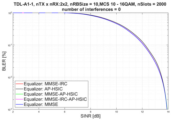
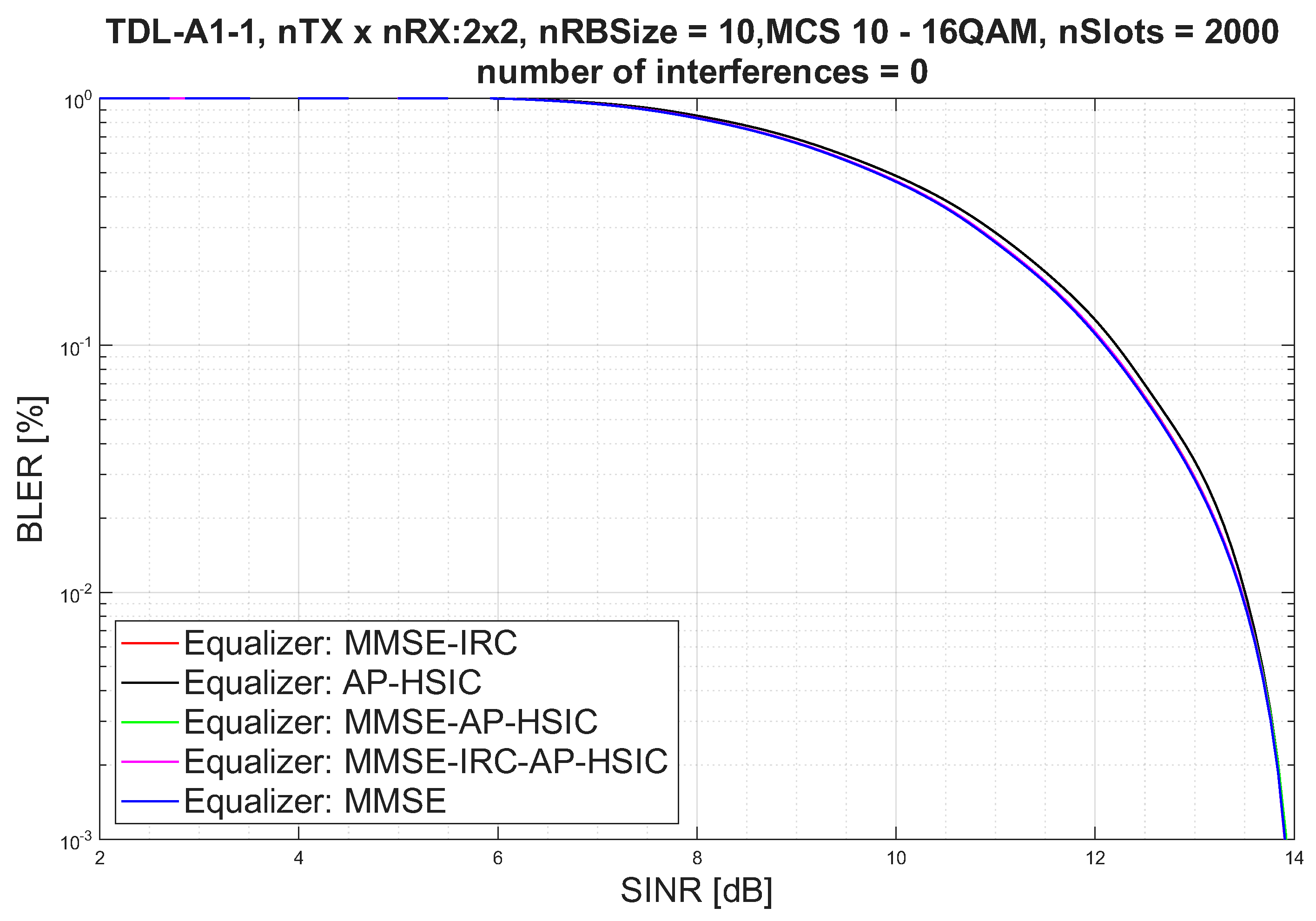
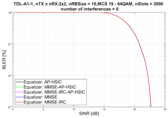
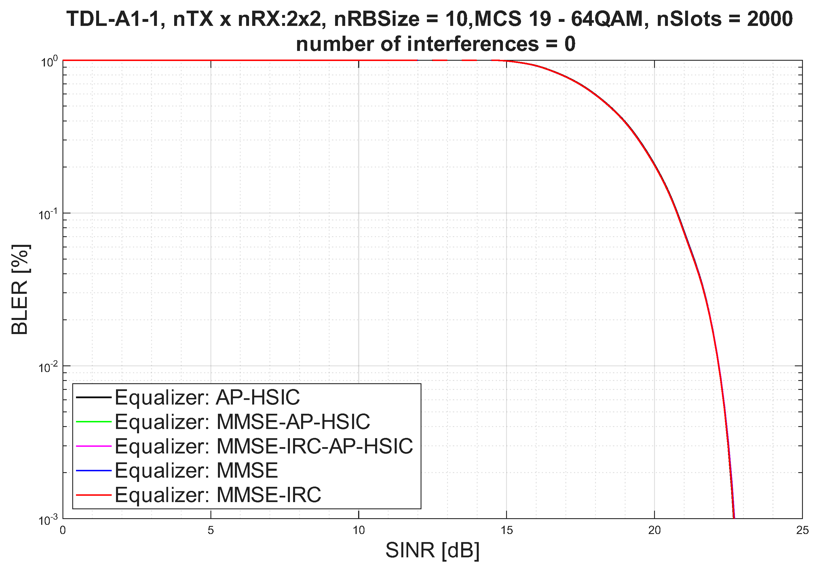
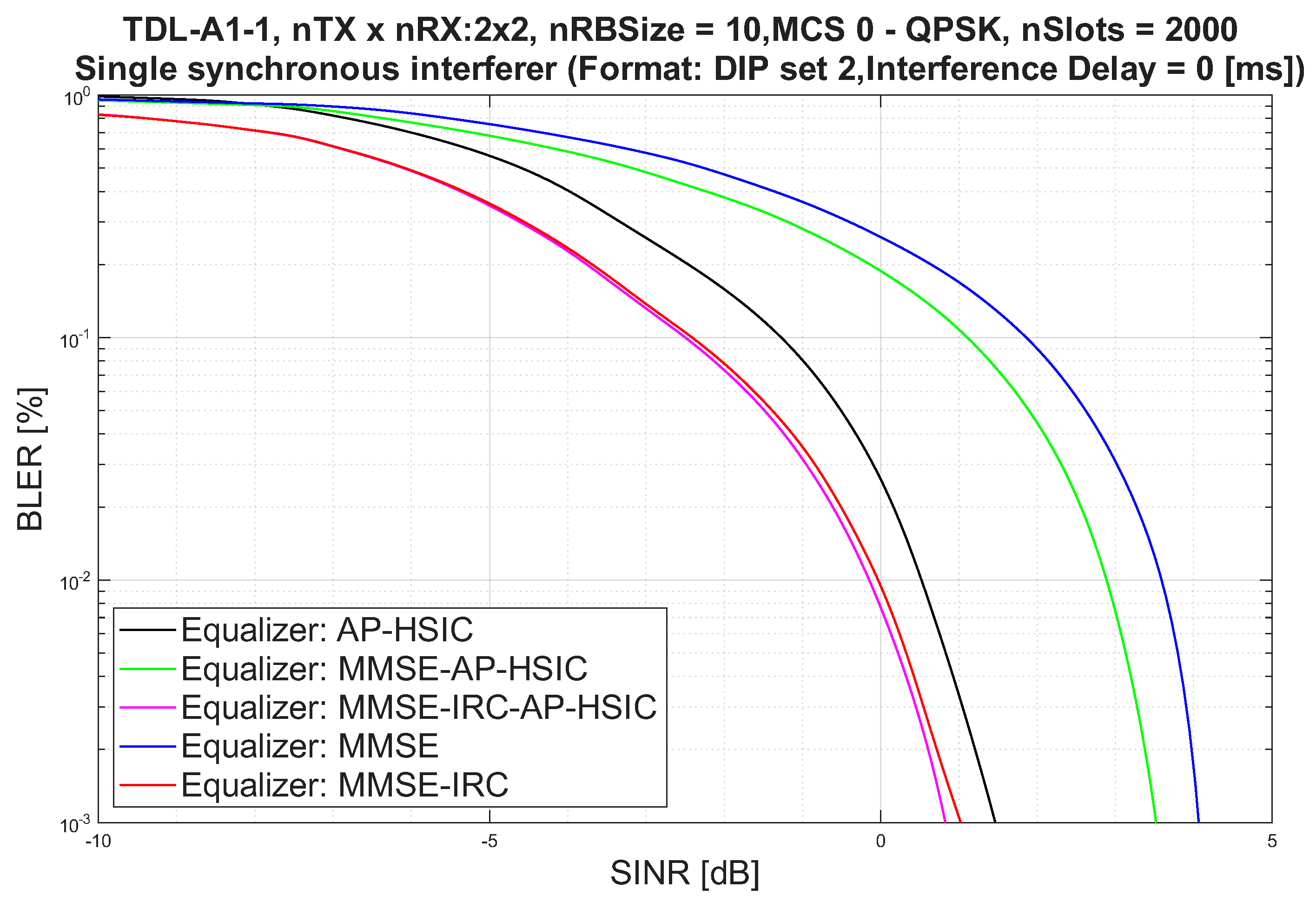
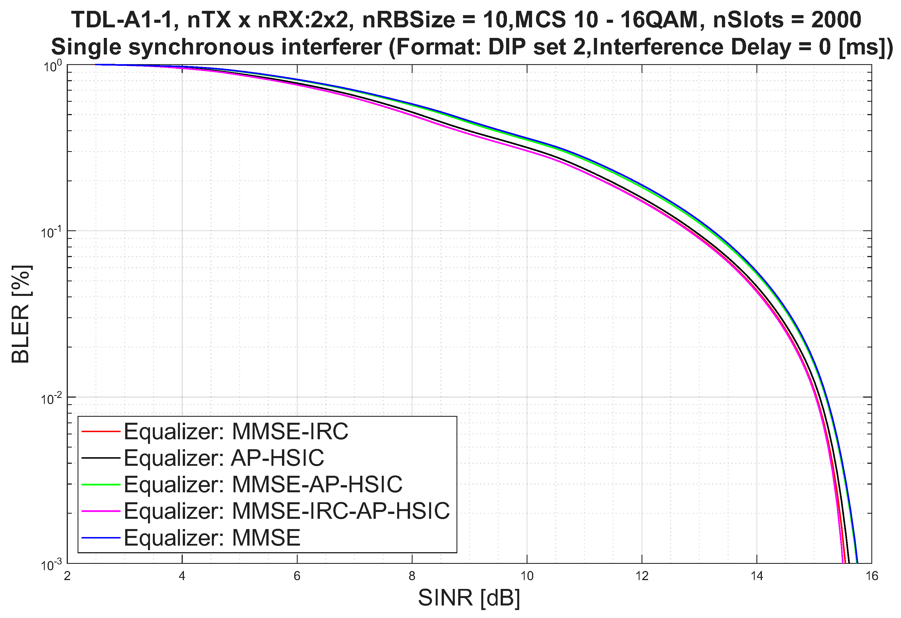
In this section, we present and discuss the PUSCH link-level simulation results for the proposed MMSE-AP-HSIC and MMSE-IRC-AP-HSIC algorithms, compared against the classical AP-HSIC, MMSE, and MMSE-IRC equalizers. Performance is reported as BLER versus SINR for the $2\times 2$ MIMO configuration and the parameters summarized in Table 3. We organize the results into three scenarios of increasing severity: (i) a baseline scenario without inter-cell interference (Figure 2, Figure 3 and Figure 4), (ii) an ICI scenario with a time-synchronized interferer (Figure 5, Figure 6 and Figure 7), and (iii) an ICI scenario with a time-asynchronous interferer (Figure 8, Figure 9 and Figure 10). Within each scenario, the QPSK, 16-QAM, and 64-QAM modulations are evaluated to span low, medium, and high spectral-efficiency operating points, respectively.

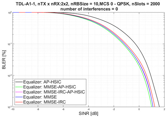
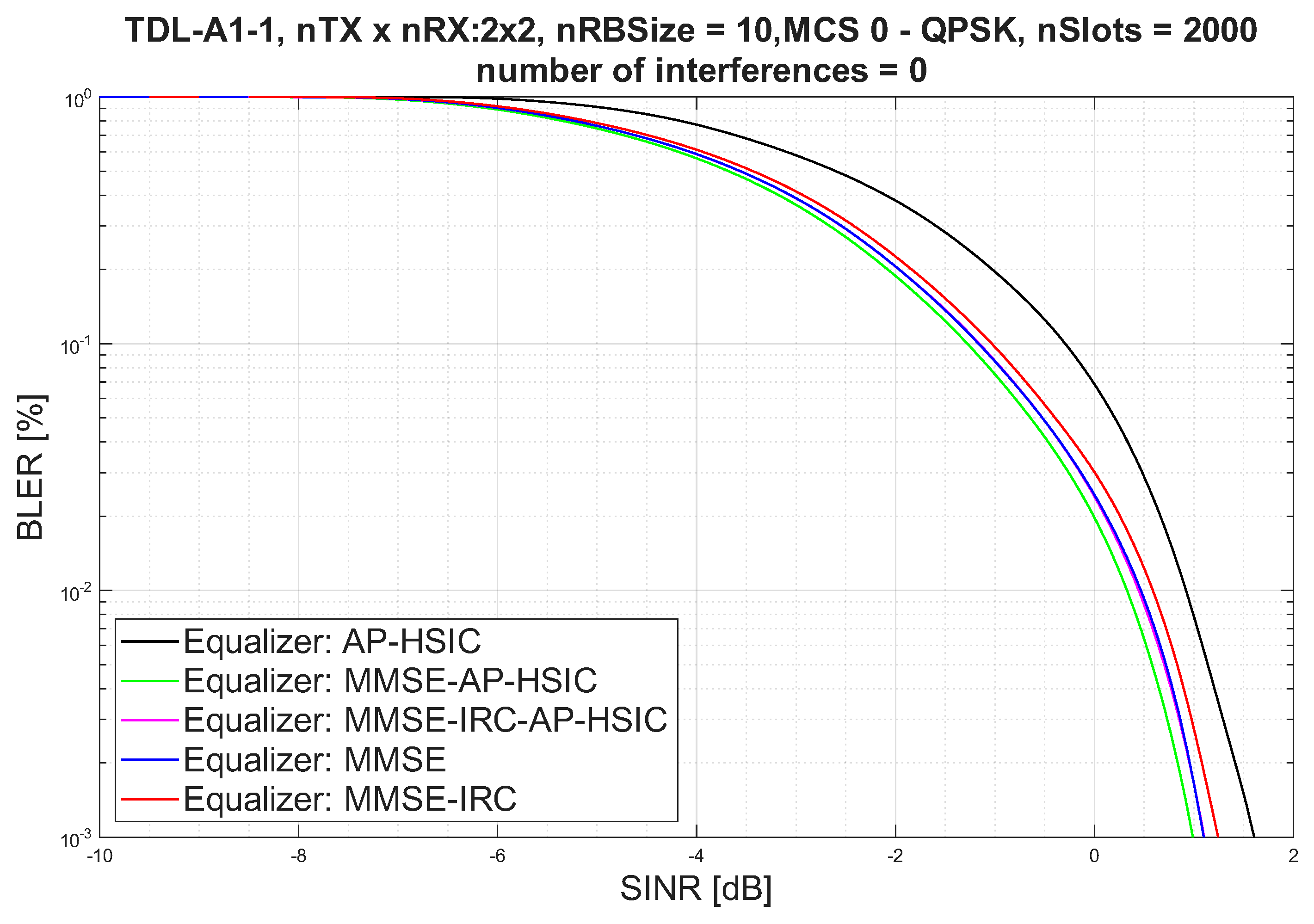
Figure 2. BLER versus SINR without inter-cell interference, QPSK modulation. MMSE-AP-HSIC improves the operating point by about 0.25 dB, while the remaining four receivers perform almost identically.

Figure 3. BLER versus SINR without inter-cell interference, 16-QAM modulation. At this higher operating SINR, the five receivers converge to almost the same performance.

Figure 4. BLER versus SINR without inter-cell interference, 64-QAM modulation. The convergence observed for 16-QAM persists at the highest spectral efficiency considered.

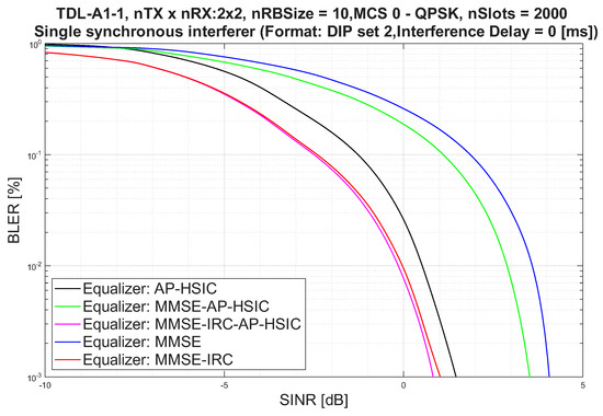
Figure 5. BLER versus SINR with a time-synchronized interferer and DIP set 2, QPSK modulation. MMSE-IRC-AP-HSIC improves on MMSE-IRC by up to 0.25 dB, while MMSE and MMSE-AP-HSIC fall well behind, including behind the conventional AP-HSIC.

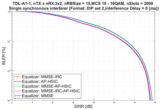
Figure 6. BLER versus SINR with a time-synchronized interferer and DIP set 2, 16-QAM modulation. The advantage of the interference-rejecting receivers over MMSE is retained, while the AP-HSIC refinement of MMSE-IRC becomes small.

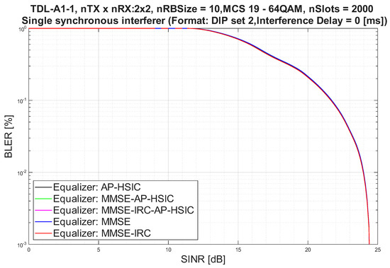
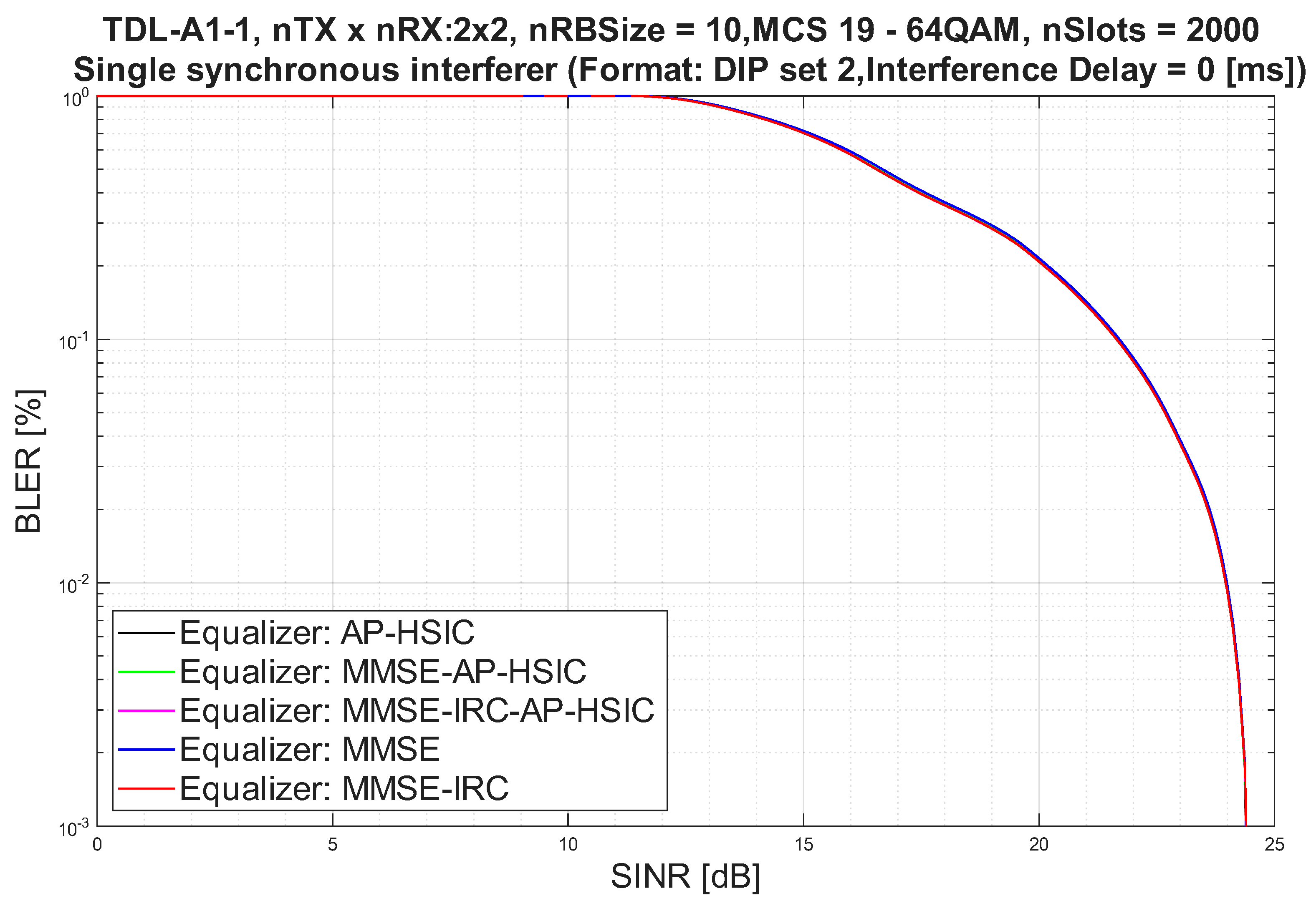
Figure 7. BLER versus SINR with a time-synchronized interferer and DIP set 2, 64-QAM modulation. The behavior observed for 16-QAM is unchanged at the highest spectral efficiency considered.

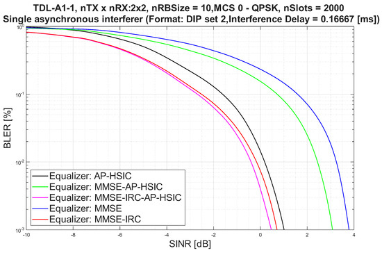
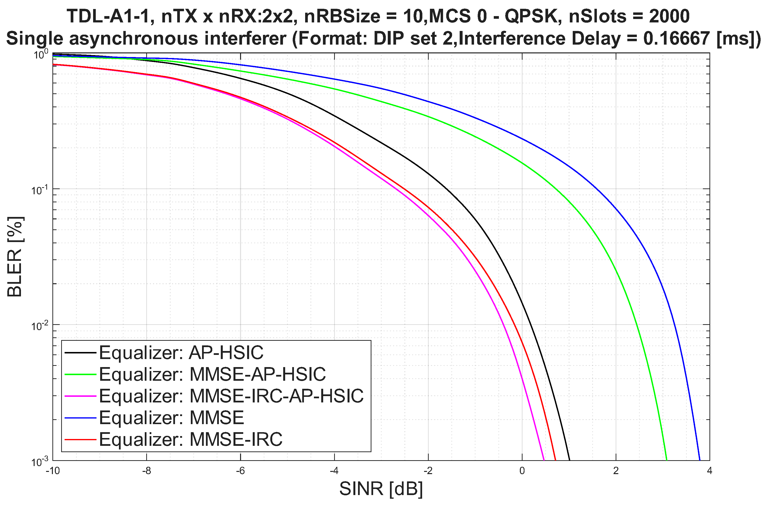
Figure 8. BLER versus SINR with a time-asynchronous interferer and DIP set 2, QPSK modulation. MMSE-IRC-AP-HSIC improves on MMSE-IRC by about 0.2 dB at $10\%$ BLER, slightly less than in the synchronized case.

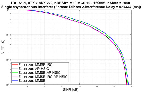
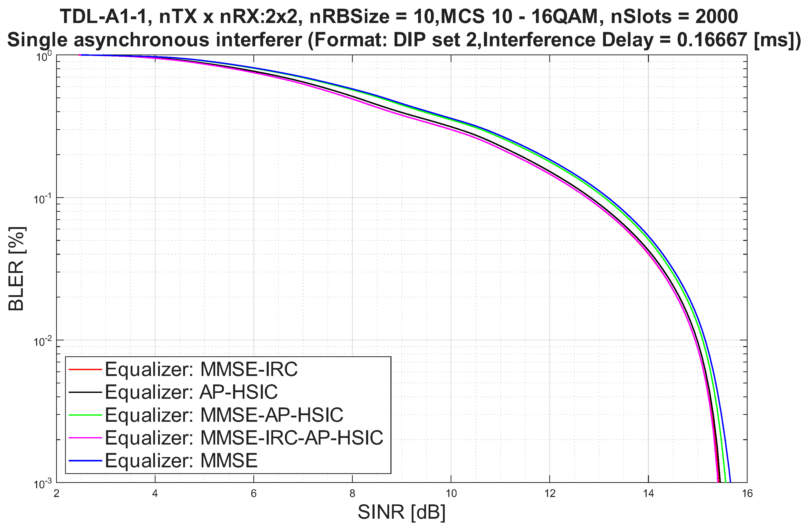
Figure 9. BLER versus SINR with a time-asynchronous interferer and DIP set 2, 16-QAM modulation. As in the synchronized case, the gain of the additional cancellation stage becomes small at this operating SINR.

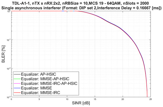
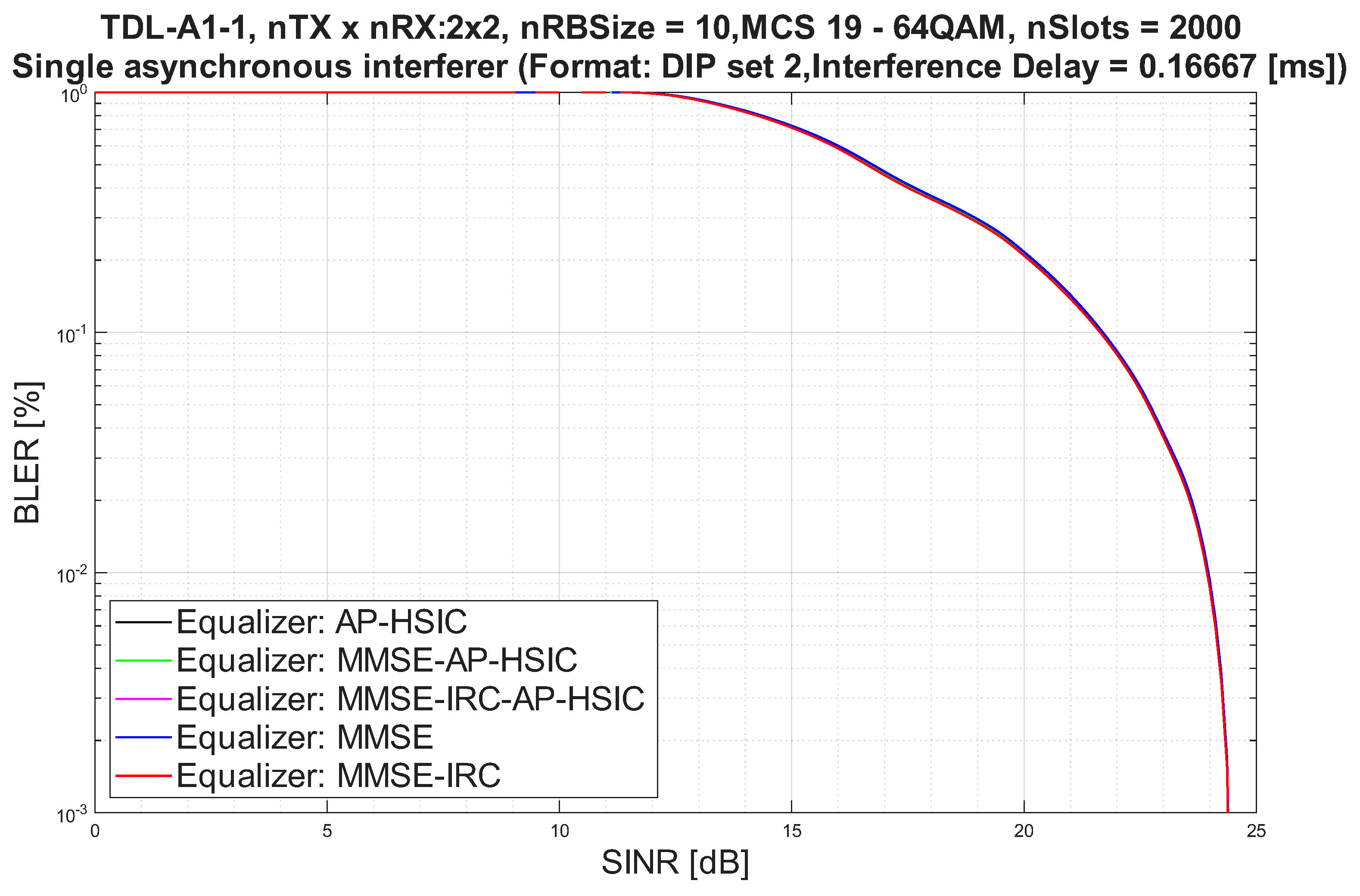
Figure 10. BLER versus SINR with a time-asynchronous interferer and DIP set 2, 64-QAM modulation. The receivers converge, as in the corresponding synchronized scenario.

In the baseline scenario without interference (Figure 2, Figure 3 and Figure 4), the second proposed algorithm, MMSE-AP-HSIC, improves performance by about 0.25 dB for QPSK modulation (see Figure 2) compared to the AP-HSIC, MMSE-IRC-AP-HSIC, and the classical MMSE and MMSE-IRC algorithms, which are known to have almost identical performance in a non-interference scenario.

In ICI scenarios with synchronized interference (DIP set 2), the proposed algorithm MMSE-IRC-AP-HSIC for interference cancellation manages to improve upon the MMSE-IRC algorithm by less than 0.25 dB for QPSK modulation (see Figure 5); the corresponding 16-QAM and 64-QAM results are shown in Figure 6 and Figure 7, respectively. The use of MMSE or MMSE-AP-HSIC receivers for this scenario results in significantly inferior performance compared to MMSE-IRC, MMSE-IRC-AP-HSIC, and even the conventional AP-HSIC algorithm. MMSE-AP-HSIC is instructive in this respect, because it applies the same alternating-projections stage as MMSE-IRC-AP-HSIC but without an interference-rejecting front end, so that the difference between the two isolates the contribution of that front end. These results emphasize the critical importance of explicit interference rejection when operating under ICI conditions.

A similar behavior is observed for non-synchronized interference with DIP set 2, where the interferer is time-asynchronous with respect to the desired signal. The proposed MMSE-IRC-AP-HSIC again outperforms the conventional MMSE-IRC for QPSK modulation, achieving an improvement of about 0.2 dB at a $10\%$ BLER (see Figure 8), while the 16-QAM and 64-QAM results are shown in Figure 9 and Figure 10, respectively.

As the assumption in our measurements is that the channel used by the various equalizers is the perfect channel, at high SINRs (16-QAM and 64-QAM) all the algorithms converge to almost the same result. This is because the effect of interference is not reflected in the channel estimation at the input to the equalizer (using a perfect channel), and the added noise and interference of the received signal are relatively low compared to QPSK.

6. Summary and Conclusions

In this paper, we proposed two new variants of the AP-HSIC equalizer, MMSE-AP-HSIC and MMSE-IRC-AP-HSIC, obtained by initializing the alternating-projections iterations with an MMSE or MMSE-IRC estimate instead of the zero-forcing solution used in [1]. The variants were evaluated against the classical AP-HSIC, MMSE, and MMSE-IRC equalizers through PUSCH link-level simulations of a $2\times 2$ MIMO uplink, across QPSK, 16-QAM, and 64-QAM and under no-interference, time-synchronized, and time-asynchronous ICI conditions.

The proposed schemes are most effective in the low-SINR, cell-edge regime. In the absence of interference, MMSE-AP-HSIC improves the QPSK operating point by about 0.25 dB over the other receivers, which otherwise perform almost identically. Under both synchronized and asynchronous ICI, MMSE-IRC-AP-HSIC outperforms the conventional MMSE-IRC for QPSK by up to 0.25 dB in the synchronized case and by about 0.2 dB at $10\%$ BLER in the asynchronous case, while MMSE and MMSE-AP-HSIC degrade sharply when the interferer is present, confirming that explicit interference rejection is essential under ICI. As the modulation order and SINR increase (16-QAM, 64-QAM), all receivers converge to nearly identical performance, as the residual noise-plus-interference becomes small relative to the signal and is not reflected in the assumed perfect channel.

These results show that the hybrid structure inherits the spatial interference-rejection capability of MMSE-IRC and refines it through iterative cancellation, combining the complementary strengths of spatial filtering and successive cancellation without requiring CSI feedback to the transmitter. From a deployment standpoint, this supports a profile-driven receiver choice rather than a uniform replacement of the existing equalizers. The measured benefit is confined to the low-SINR, QPSK cell-edge regime and amounts to 0.2–0.25 dB, with no measurable gain at 16-QAM and 64-QAM, and it is obtained at the cost of up to 21 alternating-projections iterations.

That cost, however, is incurred at the operating point where the receiver has the most computational headroom. A cell-edge user is by construction scheduled with a low MCS and a small frequency allocation, so the per-resource-element processing of the physical-layer chain operates on comparatively few samples, and the Low-Density Parity-Check (LDPC) decoder, which is the dominant contributor to the area and memory complexity of a 5G-NR receiver at high spectral efficiency [25], is correspondingly lightly loaded. At the high MCS and large allocations for which the rest of the chain is most heavily loaded, the iteration count of the proposed receivers falls to one, and essentially no additional cost is incurred. The additional complexity is therefore requested precisely where the receiver can afford it, which makes selective activation of the iterative stage, on the basis of the scheduled MCS and allocation size, a practical option for a real receiver implementation.

The present evaluation is deliberately confined to a $2\times 2$ configuration with a single dominant interferer, one TDL profile, and one asynchronous delay, a setting chosen to isolate the effect of the initialization under controlled and reproducible conditions. Extending it to multiple simultaneous interferers, larger antenna configurations, other TDL and CDL profiles, a range of Doppler spreads and timing offsets, power imbalance between interferers, and pilot-based channel and covariance estimation is left to future work.

References

- Elgam, A.; Peretz, Y.; Pinhasi, Y. Enhancing MIMO Spatial-Multiplexing and Parallel-Decoding under Interference by Computational Feedback. Electronics 2023, 12, 761. [Google Scholar] [CrossRef] [Scilit]
- Biglieri, E.; Calderbank, R.; Constantinides, A.; Goldsmith, A.; Paulraj, A.; Poor, H.V. MIMO Wireless Communications; Cambridge University Press: Cambridge, UK, 2007. [Google Scholar]
- Tawa, N.; Kuwabara, T.; Maruta, Y.; Ando, T.; Kaneko, T. Spatial division selectivity for high density users with millimeter-wave massive collocated-and distributed-MIMO. In Proceedings of the 2023 IEEE/MTT-S International Microwave Symposium-IMS 2023; IEEE: New York, NY, USA, 2023; pp. 44–47. [Google Scholar]
- Goldsmith, A. Wireless Communications; Cambridge University Press: Cambridge, UK, 2005. [Google Scholar]
- Goldsmith, A.J.; Greenstein, L.J. A measurement-based model for predicting coverage areas of urban microcells. IEEE J. Sel. Areas Commun. 2002, 11, 1013–1023. [Google Scholar]
- Marzetta, T.L.; Larsson, E.G.; Yang, H.; Ngo, H.Q. Fundamentals of massive MIMO; Cambridge University Press: Cambridge, UK, 2016. [Google Scholar]
- Lu, L.; Li, G.Y.; Swindlehurst, A.L.; Ashikhmin, A.; Zhang, R. An overview of massive MIMO: Benefits and challenges. IEEE J. Sel. Top. Signal Process. 2014, 8, 742–758. [Google Scholar] [CrossRef] [Scilit]
- Kim, H.; Kim, J.; Hong, D. Dynamic TDD systems for 5G and beyond: A survey of cross-link interference mitigation. IEEE Commun. Surv. Tutor. 2020, 22, 2315–2348. [Google Scholar] [CrossRef] [Scilit]
- Shen, Z.; Khoryaev, A.; Eriksson, E.; Pan, X. Dynamic uplink-downlink configuration and interference management in TD-LTE. IEEE Commun. Mag. 2012, 50, 51–59. [Google Scholar] [CrossRef] [Scilit]
- Elijah, O.; Leow, C.Y.; Rahman, T.A.; Nunoo, S.; Iliya, S.Z. A comprehensive survey of pilot contamination in massive MIMO—5G system. IEEE Commun. Surv. Tutor. 2015, 18, 905–923. [Google Scholar] [CrossRef] [Scilit]
- Hesketh, T.; Li, P.; de Lamare, R.C.; Wales, S. Multi-feedback successive interference cancellation with dynamic log-likelihood-ratio based reliability ordering. In Proceedings of the ISWCS 2013; The Tenth International Symposium on Wireless Communication Systems; VDE: Offenbach am Main, Germany, 2013; pp. 1–5. [Google Scholar]
- Li, P.; De Lamare, R.C.; Fa, R. Multiple feedback successive interference cancellation detection for multiuser MIMO systems. IEEE Trans. Wirel. Commun. 2011, 10, 2434–2439. [Google Scholar] [CrossRef] [Scilit]
- Van Luong, T.; Shlezinger, N.; Xu, C.; Hoang, T.M.; Eldar, Y.C.; Hanzo, L. Deep learning based successive interference cancellation for the non-orthogonal downlink. IEEE Trans. Veh. Technol. 2022, 71, 11876–11888. [Google Scholar] [CrossRef] [Scilit]
- Shlezinger, N.; Fu, R.; Eldar, Y.C. DeepSIC: Deep soft interference cancellation for multiuser MIMO detection. IEEE Trans. Wirel. Commun. 2020, 20, 1349–1362. [Google Scholar] [CrossRef] [Scilit]
- Davydov, A.; Sergeev, V.; Mondal, B.; Papathanassiou, A.; Sengupta, A. Robust MMSE-IRC for uplink massive MIMO aided C-RAN network. In Proceedings of the 2020 IEEE Globecom Workshops (GC Wkshps); IEEE: New York, NY, USA, 2020; pp. 1–5. [Google Scholar]
- Molisch, A.F.; Ratnam, V.V.; Han, S.; Li, Z.; Nguyen, S.L.H.; Li, L.; Haneda, K. Hybrid beamforming for massive MIMO: A survey. IEEE Commun. Mag. 2017, 55, 134–141. [Google Scholar] [CrossRef] [Scilit]
- Wu, S.H.; Chiu, L.K.; Wang, J.W. Reconfigurable hybrid beamforming for dual-polarized mmWave MIMO channels: Stochastic channel modeling and architectural adaptation methods. IEEE Trans. Commun. 2017, 66, 741–755. [Google Scholar] [CrossRef] [Scilit]
- Alkhateeb, A.; Leus, G.; Heath, R.W. Multi-layer precoding: A potential solution for full-dimensional massive MIMO systems. IEEE Trans. Wirel. Commun. 2017, 16, 5810–5824. [Google Scholar] [CrossRef] [Scilit]
- Xue, J.; Liang, Y.; Li, T.; Ji, W.; Li, F. User Grouping Based Multi-Layer Precoding for Multi-Cell 3D MIMO System with Statistical CSI. In Proceedings of the 2019 15th International Wireless Communications & Mobile Computing Conference (IWCMC); IEEE: New York, NY, USA, 2019; pp. 1625–1629. [Google Scholar]
- Ezri, D.; Tsodik, G. The impact of synchronization on receive beamforming with null steering in ofdm mimo systems. In Proceedings of the 2012 IEEE 27th Convention of Electrical and Electronics Engineers in Israel; IEEE: New York, NY, USA, 2012; pp. 1–4. [Google Scholar]
- Yang, S.; Chen, P.; She, X.; Liang, L.; Yang, B. Interference modeling and performance evaluation for BS MMSE-IRC receiver in LTE-A release 13. In Proceedings of the 2016 19th International Symposium on Wireless Personal Multimedia Communications (WPMC); IEEE: New York, NY, USA, 2016; pp. 239–243. [Google Scholar]
- 3GPP. 3GPP TS 36.141 V15.3.0 (2018-12): Evolved Universal Terrestrial Radio Access (E-UTRA)—Base Station (BS) Conformance Testing, 2018. 3GPP Release 15. Available online: https://www.etsi.org/deliver/etsi_ts/136100_136199/136141/15.03.00_60/ts_136141v150300p.pdf (accessed on 5 July 2026).
- 3GPP. 3GPP TS 38.211 V16.10.0 (2023-10): 5G NR—Physical Channels and Modulation, 2023. 3GPP Release 16. Available online: https://www.etsi.org/deliver/etsi_ts/138200_138299/138211/16.10.00_60/ts_138211v161000p.pdf (accessed on 5 July 2026).
- Xu, H.; Liu, Y.; Lv, G.; Yan, H. A Review of Heterogeneous Network Convergence Technology and Development Trends. In Proceedings of the 2025 7th International Conference on Next Generation Data-driven Networks (NGDN); IEEE: New York, NY, USA, 2025; pp. 45–49. [Google Scholar]
- Ren, Y.; Harb, H.; Shen, Y.; Balatsoukas-Stimming, A.; Burg, A. A Generalized Adjusted Min-Sum Decoder for 5G LDPC Codes: Algorithm and Implementation. IEEE Trans. Circuits Syst. I Regul. Pap. 2024, 71, 2911–2924. [Google Scholar] [CrossRef] [Scilit]
Disclaimer/Publisher’s Note: The statements, opinions and data contained in all publications are solely those of the individual author(s) and contributor(s) and not of MDPI and/or the editor(s). MDPI and/or the editor(s) disclaim responsibility for any injury to people or property resulting from any ideas, methods, instructions or products referred to in the content. |
© 2026 by the authors. Licensee MDPI, Basel, Switzerland. This article is an open access article distributed under the terms and conditions of the Creative Commons Attribution (CC BY) license.