CA-MC-Transformer: An Operating Condition-Adaptive and Multi-Scale Convolution-Enhanced Transformer Architecture for Furnace Temperature Prediction

Abstract

Regenerative aluminum melting serves as a core process in recycled aluminum production. In the regenerative aluminum melting process, the furnace temperature is a key variable which affects product performance and energy costs. The extreme in-furnace temperature necessitates sensors equipped with protective jackets, which increases measurement costs and severely compromises real-time monitoring capability. Accordingly, accurate furnace temperature prediction is highly valuable for regenerative aluminum melting. In regenerative aluminum melting furnaces, periodic burner nozzle commutation and frequent material charging and discharging lead to complex and time-varying operating conditions, posing considerable challenges to high-precision furnace temperature prediction. To address these issues, a condition-adaptive multi-scale convolution-enhanced Transformer (CA-MC-Transformer) model is proposed for furnace temperature prediction. Firstly, an agglomerative hierarchical clustering algorithm based on the weighted dynamic time warping (WDTW) distance is designed to perform unsupervised clustering on historical process data, thereby extracting physically interpretable prior labels for macroscopic operating conditions. Secondly, multi-scale dilated causal convolutions are utilized to capture local dynamic features at diverse temporal resolutions. A soft attention mechanism is further introduced to dynamically assign fusion weights to condition embeddings and local features, enabling condition-adaptive feature reconstruction. Finally, the fused adaptive features are fed into an encoder-only Transformer network to capture the global long-range temporal dependencies and achieve accurate furnace temperature prediction. Comparative experiments conducted on real operational datasets from an aluminum plant verify that the proposed method effectively eliminates the inherent tracking lag of conventional deep learning models, and substantially improves prediction accuracy and anti-noise robustness under complex and variable operating conditions.

1. Introduction

Aluminum is characterized by a favorable combination of light weight, high strength, corrosion resistance, and excellent electrical and thermal conductivity. It is widely used in high-end aerospace equipment development, transportation vehicle manufacturing [1], building exterior construction, power electronic device preparation [2], as well as various industrial processing equipment and daily civilian products. Aluminum melting is a typical complex industrial process, and furnace temperature serves as a critical process variable. Conventional sensors for furnace temperature measurement require protective jackets, which prevents them from achieving long-term, stable online monitoring. Accurate furnace temperature prediction is therefore essential for maintaining stable production in the aluminum melting process [3]. Accurate furnace temperature prediction also constitutes the core foundation for constructing a digital twin system of aluminum melting furnaces, as it provides real-time, high-fidelity virtual mapping of the physical melting process. In regenerative aluminum melting furnaces, factors including periodic reversing of burner nozzles result in diverse operating conditions throughout the melting process, which means the aluminum melting system cannot maintain steady operation. Furnace temperature variables show significant temporal correlation and are affected by historical operating conditions. The aluminum melting process possesses long-range time-dependent characteristics. All these challenges make it extremely difficult to establish an accurate model for the aluminum melting process.

There are primarily two methods for industrial process modeling, mechanism modeling and data-driven modeling. Mechanism modeling typically relies on principles of thermodynamics, mass and heat transfer, and kinetics. It describes the operational rules of the industrial process by establishing differential equations or state-space models, offering a certain degree of physical interpretability. In the early years, numerous scholars both domestically and internationally conducted extensive research on mechanism modeling for aluminum melting processes. These included simulations of burner layout schemes for aluminum melting furnaces [4], multi-physics field simulations inside the furnace [5], and thermodynamic simulations of aluminum melting furnaces [6]. These studies offer valuable references for the present research. Traditional mechanism-based modeling methods often encounter difficulties in model parameter identification or high computational costs due to the complexity of physical processes.

In recent years, data-driven modeling methods have become a critical technology in the field of process industries such as aluminum melting. Deep learning methods such as Recurrent Neural Networks (RNNs) [7,8,9], Convolutional Neural Networks (CNNs) [10,11,12], and Transformer [13,14,15] are widely applied across various industrial fields. In an industrial hydrocracking process, Yuan et al. [16] proposed a spatiotemporal attention-based long short-term memory (LSTM) network for soft sensor modeling to predict the initial boiling points of heavy naphtha and aviation kerosene. By incorporating spatiotemporal quality-relevant interactions, the prediction performance of the model is effectively improved. For the extraction of dynamic latent features in the debutanizer column process and industrial wastewater treatment process, a supervised bidirectional long short-term memory (SBiLSTM) network was proposed [17]. The SBiLSTM can utilize nonlinear dynamic latent information from both process variables and quality variables to improve prediction performance. To address the problem of irregular sampling frequency in data sequences from hydrocracking processes, the authors of [18] propose a Sampling Interval-Adaptive Transformer (SIA-Trans). The SIA-Trans designs an interval-aware self-attention network, feeds the processed data into the self-attention mechanism to achieve dynamic data relationship modeling, and finally outputs prediction results through a point-wise feed-forward layer. A Transformer built around the self-attention mechanism has been widely used for the continuous detection of material temperature in the melting process of medium-frequency furnaces [19]. A charge resistance data acquisition system is built on the medium-frequency furnace. By importing the resistance data inferred by the constructed resistance acquisition system into the Transformer, the temperature data of the current charge in the medium-frequency furnace can be calculated in real time. Although deep learning has achieved remarkable results in industrial process applications, two major issues persist in industrial process modeling: insufficient extraction of local features and the lack of effective modeling for furnace operating conditions. For local feature extraction, the TempreNet [20] model extracts multi-scale features through a hierarchical Transformer encoder, and combines a lightweight convolutional decoder to complete seawater temperature prediction based on multivariate observation data. The study [21] introduces convolutional sequence embedding and relative position encoding into the Transformer architecture, which improves the ability of the model to capture temporal local correlations and time-series dependencies. Simple temporal concatenation is performed during feature fusion by this method, and heterogeneous features cannot be dynamically fused. He et al. [22] proposed a prediction framework combining patch-decomposition temporal convolutional networks and Transformer, which considerably raises the prediction accuracy of industrial soft-sensing tasks. For the modeling of operating conditions, ref. [23] constructs a prediction framework integrating operating condition monitoring data and operating condition information. By explicitly modeling the variations in operating conditions, it effectively improves the prediction performance of the equipment’s remaining useful life. To tackle drastic operating condition fluctuations and frequent abnormal events during blast furnace production, Hua et al. [24] adopted a clustering algorithm to classify data into different operating conditions and built separate prediction models for each category. Focusing on the difficulty of real-time online measurement of furnace temperature in recycled aluminum melting, Duan et al. [25] proposed an operating condition classification model for the aluminum melting process based on the dynamic time warping distance, which significantly improves the accuracy of furnace temperature prediction. The study provides fundamental insights for the present work, with the effect of temporal distance ignored when measuring the correlation between sequences. In summary, existing studies can extract low-dimensional features for the modeling of some industrial processes, although these works can fail to achieve an effective combination of local features and operating condition features for industrial processes.

Inspired by the aforementioned research, a novel Transformer framework for furnace temperature prediction is proposed. In terms of the overall structure, it eliminates the Transformer decoder and solely utilizes an encoder module to fit the single-step prediction of furnace temperature sequences. Furthermore, operating condition embedding information and one-dimensional causal convolution are integrated into this model, enabling local and global feature extraction. The main contributions of this paper are as follows:

• A hierarchical agglomerative clustering algorithm based on the WDTW distance is developed for operating condition clustering, by which unsupervised fine-grained grouping of historical operational data is achieved, and high-quality physical prior labels are provided for subsequent deep learning networks.
• A multi-scale dilated causal convolution architecture is designed to extract local high-dimensional features across different time resolutions while ensuring causality. In the feature fusion stage, a soft attention mechanism is designed to deeply fuse the extracted multi-scale convolutional features with operating condition embedding vectors. Attention weight distributions specific to different operating conditions can be adaptively learned by this mechanism, and the feature representation and robustness of the method in complex and dynamic scenarios are fundamentally enhanced.
• For industrial regression tasks, the decoder module of the traditional Transformer is discarded, and a prediction network based on an encoder-only architecture is constructed. Not only is the cumulative error introduced by autoregressive decoding avoided by this network, but also the computational complexity is significantly reduced to enhance real-time performance.

2. Process Analysis of Aluminum Melting

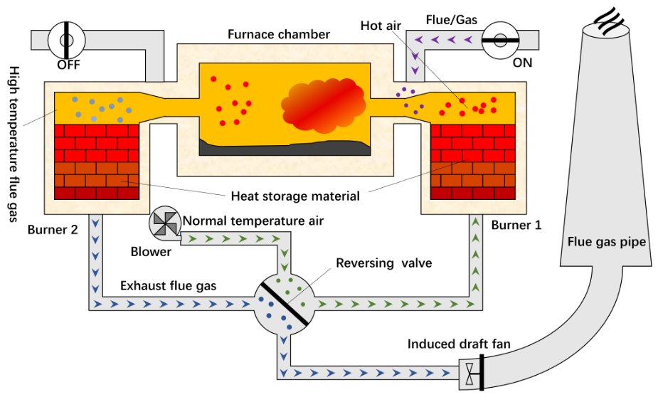
As shown in Figure 1, the regenerative aluminum melting furnace is mainly composed of a furnace chamber, regenerative burners (including regenerators, regenerative bodies, and burners), air/flue gas pipelines, reversing devices, and smoke exhaust devices. The structure of the regenerative aluminum melting furnace is closely related to its working principle; the burners come in multiple sets and integrated types. The multiple sets of burners often work alternately through reversing valves, which is key to heat recovery in the regenerative aluminum melting furnace. For a pair of regenerative burners, Burner 1 and Burner 2, when Burner 1 is in operation, its gas passage is opened, and the reversing valve is in a state that allows air to flow into the air/flue gas pipeline of Burner 1. The air is blown out by a blower and flows to the reversing valve, and then it is rapidly heated to 80–90% of the furnace temperature by the regenerator of Burner 1 before entering the furnace chamber. The preheated air temperature is around 600~900 °C. After entering the furnace chamber, the heated high-temperature air mixes with the flue gas inside, forming a lean oxygen-rich high-temperature gas flow with an oxygen content much lower than the normal 21%. At this time, gas is injected near the lean oxygen-rich high-temperature air, allowing the gas to burn in a lean oxygen state, which helps reduce the production of nitrogen oxides. Meanwhile, the other regenerative burner, Burner 2, is in the smoke exhaust and heat storage state. The gas passage of Burner 2 is closed, and the high-temperature flue gas discharged from the furnace chamber passes through the regenerator of Burner 2 and heats the regenerative body inside, storing the heat energy in the regenerative body to prepare for heating the air entering the furnace chamber when Burner 2 is in operation. After passing through the regenerative body, the high-temperature flue gas is directly discharged into the atmosphere through the reversing valve; the temperature of the flue gas discharged into the atmosphere generally does not exceed 300 °C. The flue gas from the furnace is discharged by an induced draft fan. This process is repeated in a cyclic manner, with each burner taking turns in the combustion or smoke exhaust process.

The mechanism of the aluminum melting process is complex, involving multiple variable coupling relationships; in the furnace, various physicochemical processes such as fuel combustion, heat and mass transfer, metal melting, oxidation reactions, and flue gas flow occur simultaneously. These processes not only involve multiple fields such as fluid mechanics, thermodynamics, and chemical reactions, but also exhibit significant nonlinear relationships between variables (e.g., the furnace temperature is affected by variables such as the gas flow rate, burner reversing time, and furnace pressure), making it challenging to establish an accurate mechanism model. The aluminum melting process exhibits temporal characteristics—key variables such as the furnace temperature and exhaust gas temperature often have significant time dependencies, influenced by historical operating states, and exhibit notable operational differences across different time periods. Modeling methods capable of capturing the long-term sequence dynamic characteristics are required. The aluminum melting process exhibits dynamic characteristics—it is not in a stable operating state, but undergoes continuous dynamic changes as the feeding, melting, stirring, and combustion states vary. For instance, in a regenerative aluminum melting furnace, the periodic reversal of burner nozzles causes periodic fluctuations in the furnace temperature and exhaust gas temperature. The difficulty of model establishment and prediction is increased by this complex dynamic characteristic.

Fourteen types of aluminum melting process variable data were collected, as shown in

Table 1. Process variables of aluminum melting.

No.	Variable Name	Value Range
1	Furnace temperature	102.70∼1148.00 °C
2	Material temperature	102.7∼1148 °C
3	Furnace pressure	−52.77∼129.56 Pa
4	Combustion air temperature	14∼43.6 °C
5	12# Combustion air flow	1012.66∼2065.07 Nm3/h
6	34# Combustion air flow	286.18∼7132.40 Nm3/h
7	12# Combustion air differential pressure	1424.41∼5631.80 Pa
8	34# Combustion air differential pressure	10.13∼6123.48 Pa
9	12# Gas flow	0∼443.09 Nm3/h
10	34# Gas flow	0∼503.00 Nm3/h
11	12# Air–fuel ratio	4.36∼31.46
12	34# Air–fuel ratio	2.14∼58.19
13	12# Burner reversing time	0∼41.00 s
14	34# Burner reversing time	0∼39.00 s

, including the furnace temperature, material temperature, furnace pressure, combustion air temperature, combustion air flow of 12# and 34#, combustion air differential pressure of 12# and 34#, gas flow of 12# and 34#, air–fuel ratio of 12# and 34#, and burner reversing time of 12# and 34#, where 12# and 34# represent two pairs of burners in a regenerative aluminum melting furnace.

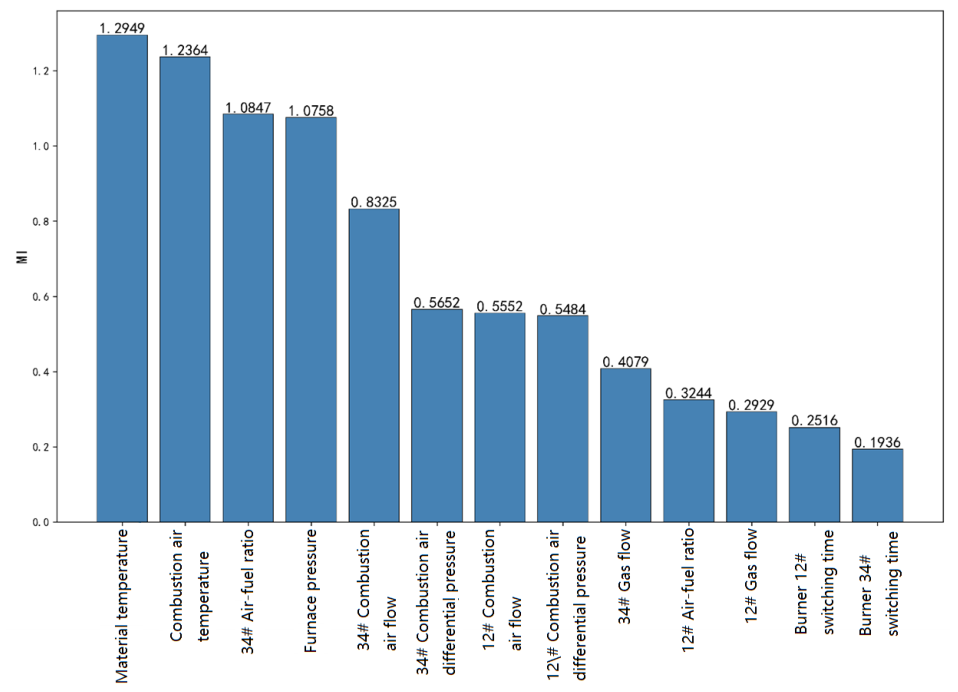
To select the key variables, the mutual information (MI) between these process variables and the target variable (furnace temperature) was calculated.

$$\mathrm{MI}(x,y)={\displaystyle \sum _{i=1}^n}{\displaystyle \sum _{j=1}^n}p\left(x_i,y_j\right)log{\displaystyle \frac{p\left(x_i,y_j\right)}{p\left(x_i\right)p\left(y_j\right)}}$$

(1)

The mutual information results are plotted in the following Figure 2, which intuitively reflects the correlation strength between each process variable and the target variable.

It can be observed from Figure 2 that the mutual information (MI) values between the furnace temperature and the two variables, i.e., the reversing time of the burner 12# and the burner 34#, are 0.2516 and 0.1936, respectively. These values are lower than those of the other variables, indicating a weak correlation with the furnace temperature variations. Consequently, these two variables can be eliminated in the subsequent training process for furnace temperature prediction.

3. The Proposed CA-MC-Transformer Model

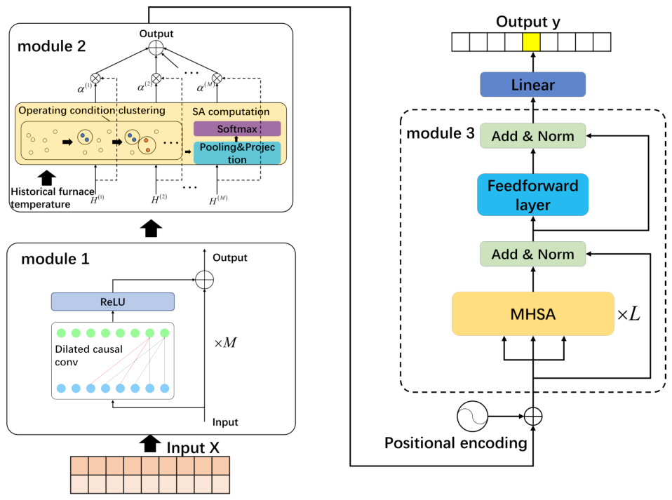
As can be seen from Figure 3, the proposed CA-MC-Transformer model consists of three modules: a time feature extraction module based on multi-scale convolution (module 1), a hierarchical clustering-based operating condition adaptation module (module 2), and a Transformer encoder module (module 3). Module 1 is introduced in Section 3.1, while module 2 and module 3 are detailed in Section 3.2 and Section 3.3.

3.1. Time Feature Extraction Module Based on Multi-Scale Convolution

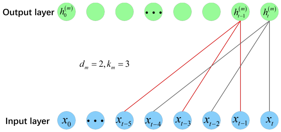
The dilated causal convolution architecture is introduced in this section, with the temporal receptive field exponentially expanded and no additional computational overhead incurred. Based on this core mechanism, a multi-scale parallel convolution branch is further constructed to achieve the refined capture of local high-dimensional features across temporal resolutions.

The structure of the dilated causal convolution is shown in Figure 4. The figure corresponds to a configuration with kernel size = 3 and dilation factor = 2. Assuming the model dimension is $F^{\prime }$, let $h_t^{\left(m\right)}\in {\mathbb{R}}^{F^{\prime }}$ denote the output of the m-th branch at time t, which is calculated as follows.

$$h_t^{\left(m\right)}={\displaystyle \sum _{i=0}^{k_m-1}}{W}_i^{\left(m\right)}·x_{t-d_m·i}+b_i^{\left(m\right)}$$

(2)

where $W_i^{\left(m\right)}\in {\mathbb{R}}^{F^{\prime }\times F}$ is the weight matrix, $b_i^{\left(m\right)}\in {\mathbb{R}}^{F^{\prime }}$ is the bias vector. $k_m$ is the convolution kernel size, which is used to map the input features from the original F-dimensional space to the $F^{\prime }$-dimensional output space. $x_{t-d_m·i}\in {\mathbb{R}}^F$ represents the value of the input sequence at the corresponding time step, and the dilation factor $d_m$ controls the sampling interval to achieve “sparse perception” of the time series. As $d_m$ increases, the convolution kernel can cover a longer time range of input information, which enhances the modeling capability for long-term dependencies. Meanwhile, the receptive field size of the model can be expressed as

$$R_m=(k_m-1)·d_m+1$$

(3)

3.2. Hierarchical Clustering-Based Operating Condition Adaptation Module

After multi-scale local features are extracted through the aforementioned work, an operating condition adaptive partitioning method based on temporal hierarchical clustering is innovatively introduced in this section, in which time-series similarity is adopted as the measurement benchmark to achieve the unsupervised fine grouping of historical data.

3.2.1. Weighted Dynamic Time Warping Distance

To better measure temporal similarity, a weighted dynamic time warping (WDTW) metric mechanism was constructed based on the classic dynamic time warping (DTW) algorithm. By assigning higher representation weights to adjacent matching points in the time dimension and imposing strict weight decay on distant matching points with large-span distortions, the pathological matching issues caused by excessive warping are effectively mitigated, and the similarity measurement results are further enabled to precisely focus on the core local evolutionary dynamics. The proposed WDTW distance algorithm is as follows.

Step 1. Given two sequences $x={\left\{x_i\right\}}_{i=1}^n$ and $y={\left\{y_j\right\}}_{j=1}^m$, where i and j are time indices, and n and m are sequence lengths. First, construct an $n\times m$ local distance matrix D,

$$D=\left(\begin{array}{ccc}d(x_1,y_1)& \cdots & d(x_1,y_m)\\ ⋮& \ddots & ⋮\\ d(x_n,y_1)& \cdots & d(x_n,y_m)\end{array}\right)$$

(4)

where each element is the local distance d, representing the local similarity between the two time series at each time point, and the local distance is generally the Euclidean distance.

$$d\left(x_i,y_j\right)=\left|x_i-y_j\right|$$

(5)

Step 2. Introduce a weight mechanism to give greater influence to the alignment of important time points. Obtain the weight matrix W,

$$W=\left(\begin{array}{ccc}{w}_{11}& \cdots & w_{1m}\\ ⋮& \ddots & ⋮\\ w_{n1}& \cdots & w_{nm}\end{array}\right)$$

(6)

with each element $w_{ij}$ in the weight matrix W defined as a function of the temporal distance, representing the weight between time points i and j.

$$w_{ij}=e^{-\mu |i-j|}$$

(7)

where e is the base of the natural logarithm, $\mu$ is the parameter controlling the weight decay rate, and $|i-j|$ represents the distance between time points. The exponential decay weight is designed based on the temporal locality assumption of industrial time series. For aluminum melting temperature sequences, the thermal state at adjacent time steps has a stronger correlation and reference value, while long-span cross-alignment easily introduces pathological warping that deviates from the physical evolution law. The exponential decay form can naturally impose smooth weight attenuation with increase in the temporal distance, which is widely adopted in weighted DTW variants for industrial time-series analysis. The value of $\mu$ is determined via grid search on the validation set, with the clustering performance (Silhouette Coefficient) as the optimization objective. The final selected value ensures the best balance between alleviating pathological alignment and retaining sequence morphological information. Then, the local distance is weighted to obtain the weighted local distance $d_w$,

$$d_w\left(x_i,y_j\right)=w_{ij}d\left(x_i,y_j\right)$$

(8)

If written in matrix form, it is the weighted local distance matrix $D^{\prime }$.

$$D^{\prime }=W\odot D=\left(\begin{array}{ccc}{w}_{11}d(x_1,y_1)& \cdots & w_{1m}d(x_1,y_m)\\ ⋮& \ddots & ⋮\\ w_{n1}d(x_n,y_1)& \cdots & w_{nm}d(x_n,y_m)\end{array}\right)$$

(9)

Step 3. Generally, there are multiple warping paths P. To calculate the DTW distance, it is necessary to find an optimal warping path $p^{\prime }={\left\{p_k\right\}}_{k=1}^K\in P$, where $p_k=(i_k,j_k)$ is the position of the k-th node on this warping path within the distance matrix, which also represents the matching relationship between $(x_i,y_j)$. K is the number of nodes on the path, satisfying $max(n,m)\le K\le n+m-1$. By minimizing the cumulative distance between sequences along the optimal warping path, the WDTW distance can be obtained.

$$WDTW(x,y)=\underset{P}{min}{\displaystyle \sum _{k=1}^K}{D}^{\prime }\left(p_k\right)$$

(10)

Step 4. Before searching for the optimal path, it is necessary to clarify the three conditions that effective curved path nodes must satisfy, including the boundary condition, monotonicity, and continuity.

• Boundary condition. The dynamic warping path must satisfy that the starting and ending points of the sequences are located at the diagonally opposite corners. That is, $p_1=(1,1)$ and $p_K=(n,m)$.
• Monotonicity. The path indices must increase monotonically, and the temporal order cannot be reversed, ensuring that the alignment process conforms to temporal causality. That is, given $p_k=(i_k,j_k)$ and $p_{k+1}=(i_{k+1},j_{k+1})$, they must satisfy $i_{k+1}\ge i_k$ and $j_{k+1}\ge j_k$.
• Continuity. Each step of the path can only move to adjacent grid points (assuming the starting point is at the top-left corner, the movement can be to the right, downward, or to the bottom-right), with a maximum step size of 1. That is, $p_{k+1}-p_k\in \{(0,1),(1,0),(1,1)\}$.

To find the minimum path, a cumulative distance matrix $D^{″}$ is constructed using dynamic programming. The cumulative distance of each node $(i,j)$ is equal to the weighted local distance of the current point plus the minimum cumulative distance of its three adjacent predecessor nodes. The recursive equation is as follows:

$$D^{″}(i,j)=D^{\prime }(i,j)+min\left\{\begin{array}{c}{D}^{″}(i-1,j)\hfill \\ D^{″}(i,j-1)\hfill \\ D^{″}(i-1,j-1)\hfill \end{array}\right.$$

(11)

where $D^{″}(0,0)=0$, and $D^{″}(i,0)=D^{″}(0,j)=\infty$. The final weighted DTW distance is obtained as

$$WDTW(x,y)=D^{″}(n,m)$$

(12)

3.2.2. Hierarchical Agglomerative Clustering Based on the WDTW Distance

After obtaining the WDTW matrix, an Agglomerative Hierarchical Clustering algorithm based on Weighted Dynamic Time Warping (AHC-WDTW) is proposed. In this algorithm, a bottom-up greedy merging strategy is adopted, the need for predefining the number of clusters is eliminated, and the hierarchical topological relationships among different time-series samples can be intuitively presented via the generated dendrogram. The specific process of the AHC-WDTW is as follows.

Step 1. Perform the initialization operation for cluster partitioning. Treat each time series in the dataset as an independent cluster, $C_i={\left\{S_i\right\}}_{i=1}^N$, where N is the number of sequences. From this, calculate the initial distance matrix. Iterate through all initial clusters, use the WDTW distance formula to calculate the distance between pairwise sequences, and construct an $N\times N$ symmetric distance matrix $D_M$. The element $D_M(i,j)$ in the matrix is the WDTW distance between sequence $S_i$ and sequence $S_j$,

$$D_M=\left(\begin{array}{ccc}\mathrm{WDTW}(S_1,S_1)& \cdots & \mathrm{WDTW}(S_1,S_N)\\ ⋮& \ddots & ⋮\\ \mathrm{WDTW}(S_N,S_1)& \cdots & \mathrm{WDTW}(S_N,S_N)\end{array}\right)$$

(13)

Step 2. Find and merge the most similar clusters. In the current distance matrix (excluding the self-distances on the diagonal), find the two clusters with the minimum distance (highest similarity). Assuming these two clusters are $C_u$ and $C_v$, they are merged into a new cluster $C^{\prime }=C_u\cup C_v$. At this point, the total number of clusters is reduced by 1.

Step 3. Update the distance matrix. Delete the rows and columns corresponding to the original clusters $C_u$ and $C_v$ in the distance matrix, and add a new row and column to represent the new cluster $C^{\prime }$. Recalculate the distances between the new cluster and all remaining clusters $C_k$, and fill them into the updated matrix. The most widely used average distance is selected to calculate the inter-cluster distance,

$$\overline{D}(C^{\prime },C_k)={\displaystyle \frac{{\sum }_{X\in C^{\prime }}{\sum }_{Y\in C_k}\mathrm{WDTW}(X,Y)}{|C^{\prime }|·|C_k|}}$$

(14)

Step 4. Termination condition check. Examine the current number of remaining clusters. If all sequences have been merged into a single giant cluster, i.e., the number of clusters is $K=1$, the algorithm terminates and outputs the final cluster assignment results. Then, based on the inter-cluster distances and hierarchical relationships during each merge, a hierarchical clustering dendrogram is plotted for subsequent truncation analysis and pattern evaluation. Otherwise, return to Step 3 to continue the iterative merging.

3.2.3. Soft Attention Mechanism

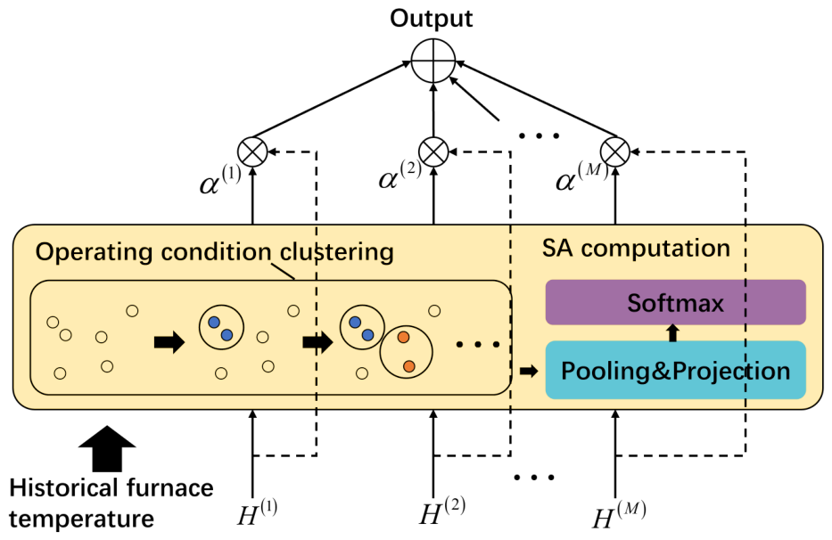
To better fuse the previously extracted multi-scale convolutional features and operating condition embedding features, the soft attention (SA) mechanism is introduced in this subsection. The principle of the soft attention mechanism is illustrated in Figure 5.

First, the multi-scale features extracted by parallel convolutions are aggregated and compressed. $H^{\left(m\right)}\in {\mathbb{R}}^{T\times F^{\prime }}$ is the feature matrix output by the m-th convolutional branch, where T is the number of time steps, and $F^{\prime }$ is the feature dimension. To obtain the globally representative features of this branch, average pooling is performed on $H^{\left(m\right)}$ along the temporal dimension, yielding the feature vector $s^{\left(m\right)}\in {\mathbb{R}}^{F^{\prime }}$.

$$s^{\left(m\right)}={\mathrm{AvgPool}}_t\left(H^{\left(m\right)}\right)$$

(15)

Secondly, calculate the soft attention weights that incorporate prior knowledge of the operating conditions and normalize them,

$${\alpha }^{\left(m\right)}=\mathrm{Softmax}\left({\left(w^{\left(m\right)}\right)}^{\top }{s}^{\left(m\right)}+b^{\left(m\right)}\left(c\right)\right)$$

(16)

where $c\in \{1,2,\dots ,K\}$ represents the current macroscopic operating condition. In practical online prediction tasks, since the future furnace temperature sequences cannot be foreseen, the model must perform condition perception based on data within the historical observation window. Specifically, the mean sequence of all sequences within each cluster in the historical training set is extracted as the centroid sequence $S^c\in {\mathbb{R}}^T$ for that operating condition. The past sequence of length T is then used to calculate the distance against the cluster centers for operating condition matching, and the cluster index with the minimum distance is extracted as the true operating condition label at the current time step. $b^{\left(m\right)}$ is the operating condition embedding function used to map the discrete label c into the operating condition bias term specific to the m-th branch, and $w^{\left(m\right)}\in {\mathbb{R}}^{F^{\prime }}$ is a learnable weight vector.

Finally, the learned attention weights are used to perform a weighted sum on the output features of each branch, obtaining the operating condition-adaptive output feature $Y\in {\mathbb{R}}^{T\times F^{\prime }}$.

$$Y={\displaystyle \sum _{m=1}^M}{\alpha }^{\left(m\right)}{H}^{\left(m\right)}$$

(17)

3.3. Transformer Encoder Module

Once the operating condition-adaptive output features are acquired, a predictive model correlating these features with the furnace temperature needs to be established. Furnace temperature prediction is defined as a single-step-ahead regression task based on multivariate historical sequences, which eliminates the requirement for autoregressive generation of variable-length sequences. To better capture the nonlinear relationships between the furnace temperature and the output features, an encoder-only Transformer framework is adopted for modeling, thereby effectively reducing the computational cost of the model.

Since the Transformer architecture is primarily based on the self-attention mechanism, it inherently lacks the ability to perceive the positional order of elements within a sequence. It is necessary to inject positional information into the feature representation at the input layer. In this section, the operating condition-adaptive features obtained in the previous section are taken as input, and absolute positional encoding (PE) is superimposed onto them. Assuming the working dimension of the model is $d_{model}=F^{\prime }$, the time step index is $t\in [1,T]$, and the frequency scale parameter is defined as ${\omega }_j=1/{10000}^{2j/d_{model}}$ for $j\in [1,d_{model}/2]$; the expanded form of the positional encoding $PE\in {\mathbb{R}}^{T\times d_{model}}$ is as follows:

$$PE=\left(\begin{array}{ccccc}sin(1·{\omega }_1)& cos(1·{\omega }_1)& \cdots & sin(1·{\omega }_{d_{model}/2})& cos(1·{\omega }_{d_{model}/2})\\ sin(2·{\omega }_1)& cos(2·{\omega }_1)& \cdots & sin(2·{\omega }_{d_{model}/2})& cos(2·{\omega }_{d_{model}/2})\\ ⋮& ⋮& \ddots & ⋮& ⋮\\ sin(T·{\omega }_1)& cos(T·{\omega }_1)& \cdots & sin(T·{\omega }_{d_{model}/2})& cos(T·{\omega }_{d_{model}/2})\end{array}\right)$$

(18)

Element-wise addition of the position encoding and the operating condition adaptive feature matrix yields input features containing temporal position information.

$$Z_0=Y+PE$$

(19)

For the l-th encoder layer, its input is $Z_{l-1}$. First, the query matrix Q, key matrix K, and value matrix V are generated through different linear transformations.

$$Q_i=Z_{l-1}{W}_i^Q,K_i=Z_{l-1}{W}_i^K,V_i=Z_{l-1}{W}_i^V$$

(20)

where $W_i^Q,W_i^K,W_i^V\in {\mathbb{R}}^{d_{model}\times d_k}$ are the learnable weight matrices for the i-th attention head, and $d_k$ is the feature dimension of each head.

Calculate the scaled dot-product attention score and obtain the weighted feature representation.

$${\mathrm{head}}_i=\mathrm{Attention}(Q_i,K_i,V_i)=\mathrm{Softmax}\left({\displaystyle \frac{Q_i{K}_i^{\mathrm{T}}}{\sqrt{d_k}}}\right)V_i$$

(21)

The outputs of the h independent attention heads are concatenated along the feature dimension and passed through a linear projection to obtain the final output of the Multi-Head Self-Attention module.

$$\mathrm{MHSA}\left(Z_{l-1}\right)=\mathrm{Concat}({\mathrm{head}}_1,\dots ,{\mathrm{head}}_h)W^O$$

(22)

where $W^O\in {\mathbb{R}}^{d_{model}\times d_{model}}$ is the output projection weight. To prevent network degradation and accelerate convergence, a residual connection and layer normalization are introduced to obtain the output of this sub-layer.

$$Z_l^{\prime }=\mathrm{LayerNorm}(Z_{l-1}+\mathrm{MHSA}\left(Z_{l-1}\right))$$

(23)

After deep feature extraction through L Transformer encoder layers, the model outputs the final feature matrix $Z_L\in {\mathbb{R}}^{T\times d_{model}}$, which fully integrates multi-scale local features, macroscopic operating condition priors, and global long-term dependencies. To achieve future state prediction of the furnace temperature, the output vector $Z_L^{\left(T\right)}$ of the feature matrix at the last time step T is extracted as the comprehensive state representation of the current moment. Finally, this vector is fed into a linear projection mapping module composed of a fully connected layer to output the single-step furnace temperature prediction value $\widehat{y}$ at time step T.

$$\widehat{y}=Z_L^{\left(T\right)}{w}_p+b_p$$

(24)

where $w_p,b_p\in {\mathbb{R}}^{d_{model}}$ are the projection weights and bias terms of the prediction layer. At this point, the model completes the end-to-end computational workflow from multivariate time-series input to single-step furnace temperature prediction.

4. Industrial Case

4.1. Experimental Setup

A furnace temperature dataset was collected in an aluminum plant, and the sampling frequency was once every 5 min. The dataset of 8730 time-series samples was divided in chronological order: the first 6984 samples were taken as the training set for gradient descent updates of network parameters; the subsequent 873 samples were used as the validation set for model hyperparameter optimization and overfitting prevention monitoring; and the last 873 samples served as an independent test set. This strict data partitioning method fundamentally avoids data leakage at the time-series boundaries.

All experiments were conducted under a unified hardware and software environment to ensure the reproducibility of experimental results and fairness of comparison. The specific experimental environment parameters are set as follows. In terms of hardware, the central processing unit is Intel i7-13620H, and the graphics processing unit is NVIDIA GeForce RTX 4050; in terms of software, the deep learning framework used is PyTorch 2.5, and the programming language adopted is Python 3.10.

The key hyperparameters of the proposed model (such as the number of encoder layers, kernel sizes of dilated convolutions, and dimension of hidden features) are systematically optimized via grid search based on the validation set, and the final configuration is selected according to the validation performance, which ensures the generalization ability of the model.

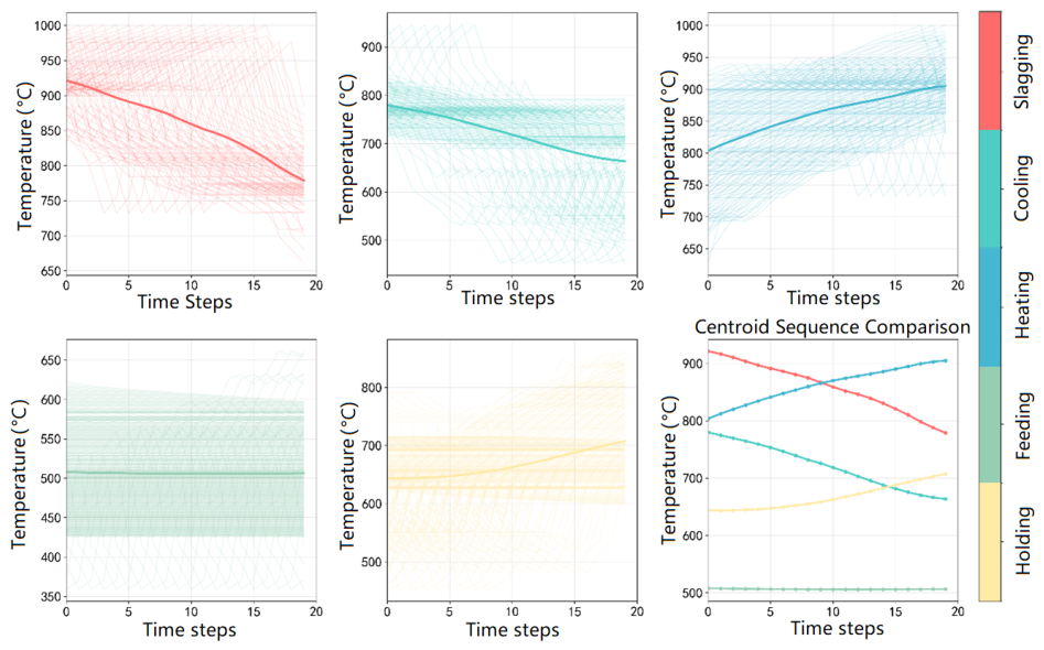
The number of clusters is determined not only by numerical evaluation metrics, but also fully incorporates domain expert knowledge of the aluminum melting process. The aluminum melting process naturally corresponds to several typical physical operating stages, including heating, holding, feeding, cooling, and slagging. The optimal number of clusters is ultimately determined to be five, which are summarized into five categories: slagging period (frequent fluctuations), cooling period (temperature drop), heating period (rapid rise), feeding period (slow rise at low temperature), and holding period (slow rise). Since the operating condition embedding is built on the basis of physical process stages, excessive adjustment of the cluster number will split or merge physically meaningful working conditions, leading to a decline in interpretability. Therefore, we focus on verifying the rationality of the selected five clusters rather than conducting a full-range sensitivity experiment. The clustering results are presented in

Table 2. Statistics of the clustering results.

Operating Condition Label	Number of Samples	Proportion
Slagging	83	9.5%
Cooling	114	13.1%
Heating	132	15.1%
Feeding	349	40.0%
Holding	195	22.3%

and Figure 6.

4.2. Results and Analysis

To evaluate the partitioning performance of the clustering algorithm on the historical operating conditions of aluminum melting, three unsupervised evaluation metrics are selected for comprehensive measurement: the Silhouette Coefficient (SC), the Calinski–Harabasz Index (CH Index), and the Davies–Bouldin Index (DBI). Assuming the number of samples is N, the specific calculation formulas are as follows:

$$\mathrm{SC}={\displaystyle \frac{1}{N}}{\displaystyle \sum _{i=1}^N}{\displaystyle \frac{b_i-a_i}{max(a_i,b_i)}}$$

(25)

where $a_i$ is the average distance from sample i to all other samples within the same cluster, and $b_i$ is the average distance from sample i to all samples in the nearest neighboring cluster.

$$\mathrm{CH}={\displaystyle \frac{\mathrm{Tr}\left(B_K\right)}{\mathrm{Tr}\left(W_K\right)}}\times {\displaystyle \frac{N-K}{K-1}}$$

(26)

where $\mathrm{Tr}\left(B_K\right)$ is the trace of the between-cluster scatter matrix, and $\mathrm{Tr}\left(W_K\right)$ is the trace of the within-cluster scatter matrix.

$$\mathrm{DBI}={\displaystyle \frac{1}{K}}{\displaystyle \sum _{i=1}^K}\underset{j\ne i}{max}\left({\displaystyle \frac{s_i+s_j}{d_{ij}}}\right)$$

(27)

In Equation (27), $s_i$ is the average distance from all samples within cluster i to its cluster center, and $d_{ij}$ is the distance between the center of cluster i and the center of cluster j.

To measure the fitting accuracy between the molten aluminum temperature $\widehat{y}$ predicted by the CA-MC-Transformer model and the true furnace temperature y, four widely used evaluation metrics are selected: Root Mean Square Error (RMSE), Mean Absolute Error (MAE), Mean Absolute Percentage Error (MAPE), and Coefficient of Determination (R²). Assuming the total number of samples in the test set is N, the predicted temperature is $\widehat{y}$ and the true temperature is y, the specific calculation equations for each metric are shown in Equations (28)–(31).

$$\mathrm{RMSE}=\sqrt{{\displaystyle \frac{1}{N}}\sum _{i=1}^N{(y_i-{\widehat{y}}_i)}^2}$$

(28)

$$\mathrm{MAE}={\displaystyle \frac{1}{N}}{\displaystyle \sum _{i=1}^N}|y_i-{\widehat{y}}_i|$$

(29)

$$\mathrm{MAPE}={\displaystyle \frac{1}{N}}{\displaystyle \sum _{i=1}^N}\left|{\displaystyle \frac{y_i-{\widehat{y}}_i}{y_i}}\right|$$

(30)

$${\mathrm{R}}^2=1-{\displaystyle \frac{{\sum }_{i=1}^N{(y_i-{\widehat{y}}_i)}^2}{{\sum }_{i=1}^N{(y_i-\overline{y})}^2}}$$

(31)

4.2.1. Comparative Experiments

To verify the effectiveness of the proposed AHC-WDTW, the clustering performance of the following clustering algorithms was compared: K-means [26], K-medoids [27], K-Shape [28], FCM [29], AHC (Euclidean distance) [30], and the proposed AHC-WDTW. Unless otherwise indicated, all clustering algorithms used the WDTW distance to measure the similarity between sequences by default. The results are shown in

Table 3. Comparison of evaluation metrics for different clustering algorithms.

Algorithm Name	Silhouette Coefficient	CH Index	DBI
K-means	0.425	1342.518	1.582
K-medoids	0.461	1485.247	1.415
K-Shape	0.584	1920.863	1.104
FCM	0.448	1405.691	1.512
AHC (Euclidean distance)	0.472	1512.355	1.386
AHC-WDTW	0.675	2354.129	0.842

Note: The best performance for each metric is highlighted in bold; the same below.

.

From the clustering evaluation metrics in Table 3, it can be observed that the proposed AHC-WDTW achieves optimal performance in all metrics, significantly overcoming the drift error of traditional algorithms in processing aluminum melting time-series data. The specific performance gains are as follows. Compared to the original K-means algorithm, the silhouette coefficient of the proposed algorith increases from 0.425 to 0.675, representing a relative improvement of 58.82%; the CH index increases from 1342.518 to 2354.129, a substantial increase of 75.35%; and the DBI decreases from 1.582 to 0.842, a reduction of 46.78%. It is implied that the morphological characteristics of the operating condition sequence can be more accurately captured by the WDTW distance. Compared to the original AHC algorithm using the Euclidean distance, the proposed algorithm, without altering the network structure, merely by replacing the distance metric, improves the silhouette coefficient by 43.01%, increases the CH index by 55.66%, and reduces the DBI by 39.25%. It is demonstrated that when complex furnace temperature conditions with varying lengths and time-axis scaling are encountered, significant advantages in similarity measurement are exhibited by using the WDTW distance, and high-quality prior labels are provided for subsequent prediction models.

To verify the effectiveness of the proposed CA-MC-Transformer, the evaluation metrics for furnace temperature prediction comparing different prediction models, LSTM [31], TCN [32], CNN-LSTM [33], Transformer (Encoder-Decoder) [13], Autoformer [14], and CA-MC-Transformer, are presented in

Table 4. Comparison of the evaluation metrics for different prediction models.

Model Name	RMSE	MAE	MAPE	R2	Params FLOPs
LSTM	18.0093 ± 0.8715	11.6427 ± 0.6934	0.0212 ± 0.0016	0.9622 ± 0.0012	1.21 M 0.22 G
TCN	15.5780 ± 1.0213	10.2643 ± 0.4256	0.0193 ± 0.0008	0.9717 ± 0.0023	1.85 M 0.35 G
CNN-LSTM	14.0972 ± 0.5581	9.5576 ± 0.7321	0.0165 ± 0.0014	0.9769 ± 0.0017	3.22 M 0.78 G
Transformer (Encoder-Decoder)	11.2671 ± 0.9427	7.7080 ± 0.2618	0.0142 ± 0.0011	0.9852 ± 0.0009	14.63 M 2.86 G
Autoformer	10.0065 ± 0.6234	7.8894 ± 0.5142	0.0127 ± 0.0005	0.9883 ± 0.0015	11.57 M 2.35 G
CA-MC-Transformer	6.5558 ± 0.3872	5.2193 ± 0.2549	0.0096 ± 0.0007	0.9950 ± 0.0006	22.15 M 4.12 G

.

The comparison experiments were independently run five times for each model to ensure statistical robustness. As can be seen from Table 4, the reported evaluation metrics are presented as mean values along with their corresponding standard deviations. Additionally, the table provides the theoretical number of model parameters (in millions) and floating-point operations (FLOPs, in giga) for each model, which serve as metrics of their respective computational complexity and model capacity. The proposed CA-MC-Transformer model demonstrates significant performance advantages across all metrics. Compared with the traditional LSTM, the proposed model substantially compresses the RMSE from 18.0093 to 6.5558, achieving an error reduction rate as high as 63.60%; the MAE decreases from 11.6427 to 5.2193, a reduction of 55.17%; and the MAPE drops from 0.0212 to 0.0096, a decrease of 54.55%, successfully controlling the relative prediction deviation to within 1%. Compared with the base Transformer, the proposed model reduces RMSE, MAE, and MAPE by 41.82%, 32.29%, and 32.23%, respectively. Compared with the Autoformer, which is optimized for time series, the RMSE of the proposed model decreases by 34.49%. The R² steadily improves from 0.9852 in the Transformer to 0.9950. The superiority of the proposed model in the furnace temperature prediction task is proved.

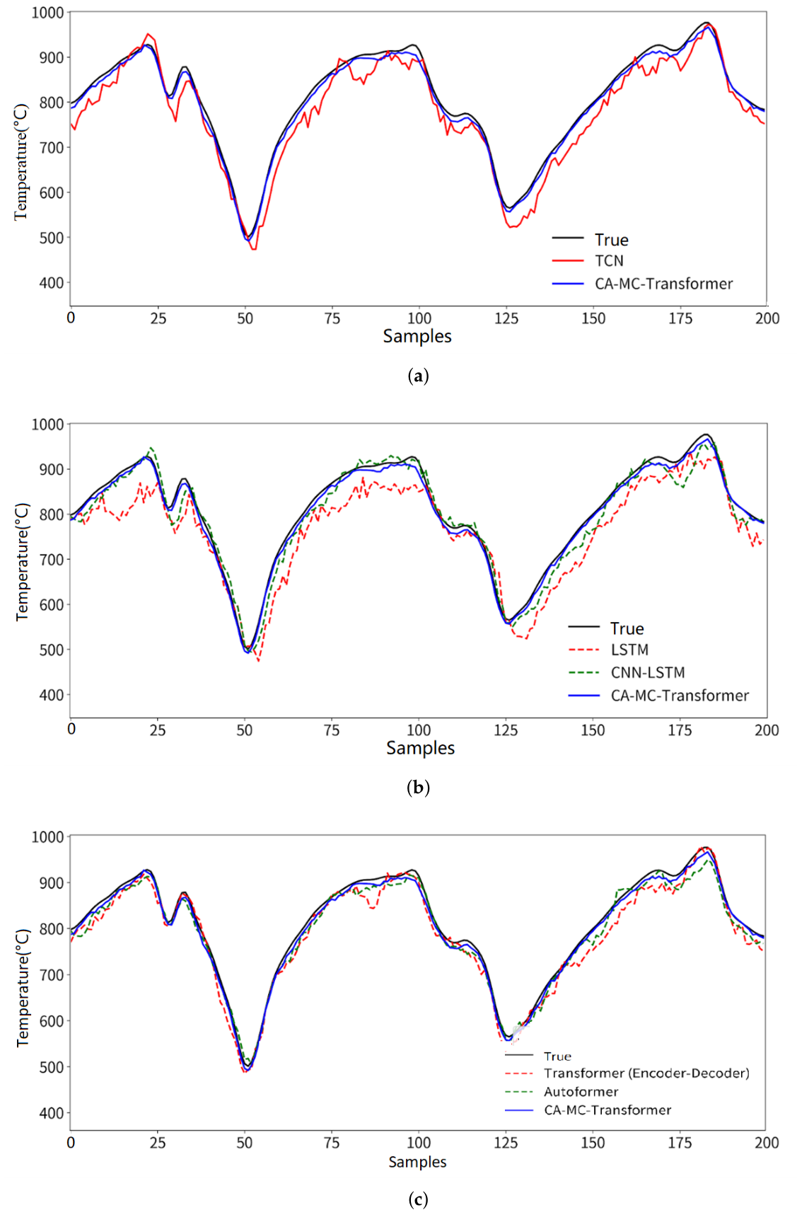
To intuitively observe the fitting accuracy of each prediction model, the comparison curves between the predicted values and the true values of the six prediction models on 200 samples in the test set are respectively plotted, and the results are shown in Figure 7.

4.2.2. Ablation Experiments

To evaluate the effectiveness of each key module in the proposed CA-MC-Transformer model, a series of ablation experiments are designed in this section. By gradually stripping or replacing core modules, the following four variant models are constructed for comparative analysis:

• MC-Transformer. The operating condition-aware embedding CA module constructed based on agglomerative hierarchical clustering is eliminated in this variant, and pure temporal data are solely relied on for feature extraction.
• CA-Transformer. In this variant, the front-end multi-scale convolutional layer (MC) is removed, and the original sliding window sequence and operating conditions are directly embedded into the encoder after being stacked.
• CA-MC-Transformer (without SA). In this variant, the soft attention mechanism is removed, and the most basic feature concatenation is employed for feature fusion.
• Transformer (Encoder). The model is degraded into a standard Transformer encoder model in this variant by simultaneously removing three major modules, namely, operating condition adaptation, soft attention, and multi-scale convolution.

The ablation experiment results of the CA-MC-Transformer model are shown in

Table 5. Ablation experiment results of the CA-MC-Transformer model.

Model Name	RMSE	MAE	MAPE	R2	Params FLOPs
MC-Transformer	10.7590 ± 0.4156	7.4371 ± 0.2984	0.0137 ± 0.0012	0.9865 ± 0.0018	12.50 M 2.10 G
CA-Transformer	9.7556 ± 0.3892	7.5280 ± 0.4135	0.0140 ± 0.0017	0.9889 ± 0.0015	11.20 M 1.90 G
CA-MC-Transformer (without SA)	8.0643 ± 0.5410	6.4025 ± 0.3021	0.0117 ± 0.0011	0.9924 ± 0.0012	15.00 M 2.80 G
Transformer (Encoder)	13.1914 ± 0.3127	9.1082 ± 0.2145	0.0168 ± 0.0008	0.9797 ± 0.0021	8.50 M 1.50 G
CA-MC-Transformer	6.5558 ± 0.3872	5.2193 ± 0.2549	0.0096 ± 0.0007	0.9950 ± 0.0006	22.15 M 4.12 G

. The results are reported as the mean ± standard deviation obtained from five ablation experiments. The table also presents the theoretical model parameters and FLOPs for each variant. The gain from the multi-scale convolutional module is as follows. Compared to the baseline Transformer (Encoder) model, the RMSE of the MC-Transformer decreased from 13.1914 to 10.7590, representing an error reduction of 18.44%, while MAE decreased by 18.35%. It is indicated that local abrupt features in furnace temperature sequences can be effectively captured by the multi-scale context.

The gain from the operating condition-adaptive perception module is as follows. After introducing the CA module alone, the RMSE of the CA-Transformer dropped from 13.1914 to 9.7556, achieving a reduction rate of 26.05%, which exceeds the improvement brought by the MC module. It is verified that a decisive influence on the variation trend of furnace temperature is exerted by different melting operating conditions.

The gain from the soft attention mechanism is as follows. When both CA and MC modules are incorporated, the RMSE of the CA-MC-Transformer (without SA) is 8.0643. Introducing the soft attention mechanism further reduces the RMSE to 6.5558—an additional decrease of 18.71%—while MAE drops by 18.48%. It is fully demonstrated that the prediction accuracy of the model is improved by dynamically assigning weights to operating condition priors and local time series via the soft attention mechanism.

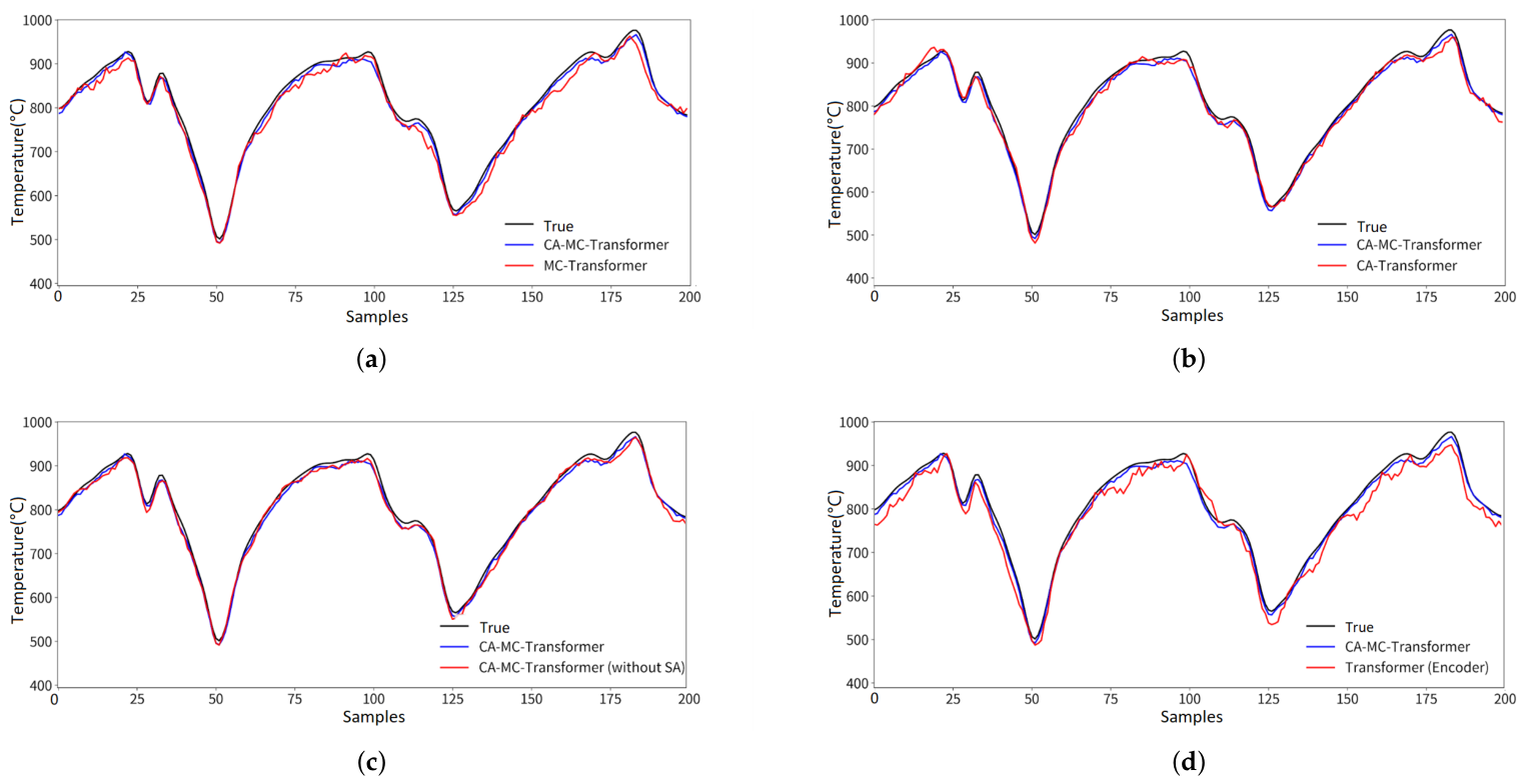
The visualization results of various variant models on 200 samples from the test set are shown in Figure 8. As illustrated, the Transformer (Encoder) exhibits the largest deviation, indicating that reliance solely on the basic Transformer encoder structure, although capable of capturing certain global dependencies, struggles to deeply uncover the multi-scale nonlinear dynamic features embedded in complex industrial time-series data. In contrast, the fitting accuracy of the MC, CA, and SA modules clearly converges toward the true values compared to the Transformer (Encoder), demonstrating that each module plays an irreplaceable role in feature extraction, attention allocation, and temporal dependency modeling. Ultimately, the complete model is enabled to achieve optimal fitting performance in the complex furnace temperature prediction task.

4.3. Discussion

The experimental results confirm that the proposed CA-MC-Transformer achieves superior prediction accuracy and robustness on the real industrial aluminum melting dataset. The performance gain stems from the collaborative optimization of three dimensions: multi-scale convolution captures local dynamic features under burner reversing and feeding disturbances; the AHC-WDTW clustering provides physically interpretable operating condition priors; and the soft attention mechanism realizes adaptive fusion of local and condition features, enabling the model to adapt to complex variable-condition scenarios. Compared with existing aluminum melting temperature prediction methods, this work fully highlights the guiding value of physical condition knowledge for data-driven modeling, and the encoder-only architecture also effectively reduces inference latency, which is more suitable for real-time industrial deployment. As a core soft-sensing module in the digital twin architecture of aluminum melting furnaces, the model provides reliable real-time state mapping to support closed-loop process optimization and intelligent production scheduling.

Nevertheless, the current work still has limitations. The model’s generalization performance on completely unseen operating conditions still needs further verification, as the current training data cover typical but not all possible extreme conditions. Key hyperparameters are optimized via grid search based on the validation set, while a full-range sensitivity analysis is not fully conducted in this work. The current method is validated on the aluminum melting furnace scenario, and its direct applicability to other industrial thermal processes with different mechanism characteristics needs further exploration. The actual end-to-end inference latency and deployment performance on industrial edge devices remain to be further verified in real deployment scenarios.

5. Conclusions

In this paper, the challenge of accurately predicting the furnace temperature in regenerative aluminum melting furnaces, which are characterized by strong nonlinearity and variable operating conditions, is addressed. To this end, a CA-MC-Transformer model for furnace temperature prediction is proposed, based on operational condition awareness and multi-scale feature fusion. First, to fully exploit prior knowledge about physical operating conditions during the aluminum melting process, an agglomerative hierarchical clustering algorithm incorporating the WDTW distance metric is introduced for clustering analysis. By clustering historical furnace temperature sequences, an operational condition-aware embedding module is constructed, effectively overcoming the limitations of traditional distance metrics in handling temporal sequence distortions and time-axis scaling. Second, a front-end multi-scale convolutional module is employed to extract local high-frequency features from the temperature sequences in parallel, along with a soft attention fusion mechanism. By this mechanism, weights are dynamically assigned to both operational condition priors and local temporal features; with both deeply integrated into the standard Transformer encoder, the ability of the model to capture dynamic changes in complex thermodynamic systems is significantly enhanced. Experimental results demonstrate that the CA-MC-Transformer model effectively overcomes the tracking lag commonly observed in traditional deep learning models. The effectiveness of the proposed modules is fully verified by quantitative analysis, and it is demonstrated that high prediction accuracy and robustness are achieved by the model in the furnace temperature prediction task.

References

1. Rohatgi, P.; Weiss, D.; Srivatsan, T.S.; Ghaderi, O.; Zare, M. Solidification Processing of Aluminum Alloy Metal Matrix Composites for Use in Transportation Applications. Metall. Mater. Trans. A 2024, 55, 4867–4881. [Google Scholar] [CrossRef] [Scilit]
2. Ogawa, F.; Osada, N.; Itoh, T.; Sakane, M. Creep Deformation and Rupture Life Characteristics of High-Purity Aluminum for High-Power Electronic Devices. J. Mater. Eng. Perform. 2025, 34, 7410–7425. [Google Scholar] [CrossRef] [Scilit]
3. Dion, L.; Kiss, L.I.; Poncsák, S.; Lagacé, C.L. Prediction of Low-Voltage Tetrafluoromethane Emissions Based on the Operating Conditions of an Aluminium Electrolysis Cell. JOM 2016, 68, 2472–2482. [Google Scholar] [CrossRef] [Scilit]
4. Wang, J.; Xu, P.; Yan, H.; Zhou, J.; Li, S.; Gui, G.; Li, W. Burner effects on melting process of regenerative aluminum melting furnace. Trans. Nonferr. Met. Soc. China 2013, 23, 3125–3136. [Google Scholar] [CrossRef] [Scilit]
5. Yan, H.; Xie, H.; Zheng, W.; Liu, L. Numerical simulation of combustion and melting process in an aluminum melting furnace: A study on optimizing stacking mode. Appl. Therm. Eng. 2024, 245, 122840. [Google Scholar] [CrossRef] [Scilit]
6. Luo, Y.; Dai, J.; Chen, X.; Liu, Y. A Hybrid Modeling Method for Aluminum Smelting Process Based on a Hybrid Strategy-Based Sparrow Search Algorithm. IEEE Access 2022, 10, 101149–101159. [Google Scholar] [CrossRef] [Scilit]
7. Caterini, A.L.; Chang, D.E. Recurrent Neural Networks. In Deep Neural Networks in a Mathematical Framework; Caterini, A.L., Chang, D.E., Eds.; Springer International Publishing: Cham, Switzerland, 2018; pp. 59–79. [Google Scholar] [CrossRef] [Scilit]
8. Salehinejad, H.; Sankar, S.; Barfett, J.; Colak, E.; Valaee, S. Recent Advances in Recurrent Neural Networks. arXiv 2018, arXiv:1801.01078. [Google Scholar] [CrossRef] [Scilit]
9. Pascanu, R.; Gulcehre, C.; Cho, K.; Bengio, Y. How to Construct Deep Recurrent Neural Networks. arXiv 2014, arXiv:1312.6026. [Google Scholar] [CrossRef] [Scilit]
10. Lin, Y.; Koprinska, I.; Rana, M. Temporal Convolutional Attention Neural Networks for Time Series Forecasting. In Proceedings of the 2021 International Joint Conference on Neural Networks (IJCNN), Shenzhen, China, 18–22 July 2021; pp. 1–8. [Google Scholar] [CrossRef] [Scilit]
11. Zheng, J.; Ma, L.; Wu, Y.; Ye, L.; Shen, F. Nonlinear Dynamic Soft Sensor Development with a Supervised Hybrid CNN-LSTM Network for Industrial Processes. ACS Omega 2022, 7, 16653–16664. [Google Scholar] [CrossRef] [Scilit] [PubMed]
12. Liu, J.; He, J.; Tang, Z.; Xie, Y.; Gui, W.; Ma, T.; Jahanshahi, H.; Aly, A.A. Frame-Dilated Convolutional Fusion Network and GRU-Based Self-Attention Dual-Channel Network for Soft-Sensor Modeling of Industrial Process Quality Indexes. IEEE Trans. Syst. Man Cybern. Syst. 2022, 52, 5989–6002. [Google Scholar] [CrossRef] [Scilit]
13. Vaswani, A.; Shazeer, N.; Parmar, N.; Uszkoreit, J.; Jones, L.; Gomez, A.N.; Kaiser, L.; Polosukhin, I. Attention is all you need. In Proceedings of the Advances in Neural Information Processing Systems, Long Beach, CA, USA, 4–9 December 2017; pp. 5998–6008. [Google Scholar]
14. Wu, H.; Xu, J.; Wang, J.; Long, M. Autoformer: Decomposition Transformers with Auto-Correlation for Long-Term Series Forecasting. arXiv 2022, arXiv:2106.13008. [Google Scholar] [CrossRef] [Scilit]
15. Nie, Y.; Nguyen, N.H.; Sinthong, P.; Kalagnanam, J. A Time Series is Worth 64 Words: Long-term Forecasting with Transformers. arXiv 2023, arXiv:2211.14730. [Google Scholar] [CrossRef] [Scilit]
16. Yuan, X.; Li, L.; Shardt, Y.A.W.; Wang, Y.; Yang, C. Deep Learning With Spatiotemporal Attention-Based LSTM for Industrial Soft Sensor Model Development. IEEE Trans. Ind. Electron. 2021, 68, 4404–4414. [Google Scholar] [CrossRef] [Scilit]
17. Lui, C.F.; Liu, Y.; Xie, M. A Supervised Bidirectional Long Short-Term Memory Network for Data-Driven Dynamic Soft Sensor Modeling. IEEE Trans. Instrum. Meas. 2022, 71, 2504713. [Google Scholar] [CrossRef] [Scilit]
18. Xu, Z.; Xu, N.; Wang, K.; Yuan, X.; Wang, Y.; Yang, C.; Gui, W.; Cheng, S.; Ye, L. A sampling interval-adaptive transformer for industrial time sequence modeling with heterogeneou s sampling rates in quality prediction. Eng. Appl. Artif. Intell. 2025, 162, 112374. [Google Scholar] [CrossRef] [Scilit]
19. Ma, S.; Li, Y.; Luo, D.; Song, T. Temperature Prediction of Medium Frequency Furnace Based on Transformer Model. In Proceedings of the Neural Computing for Advanced Applications; Zhang, H., Chen, Y., Chu, X., Zhang, Z., Hao, T., Wu, Z., Yang, Y., Eds.; Springer: Singapore, 2022; pp. 463–476. [Google Scholar] [CrossRef] [Scilit]
20. Chen, Q.; Cai, C.; Chen, Y.; Zhou, X.; Zhang, D.; Peng, Y. TemproNet: A transformer-based deep learning model for seawater temperature prediction. Ocean Eng. 2024, 293, 116651. [Google Scholar] [CrossRef] [Scilit]
21. Wen, Y.; Xu, P.; Li, Z.; Xu, W.; Wang, X. RPConvformer: A novel Transformer-based deep neural networks for traffic flow prediction. Expert Syst. Appl. 2023, 218, 119587. [Google Scholar] [CrossRef] [Scilit]
22. He, Y.L.; Bai, Z.H.; Xu, Y.; Zhu, Q.X.; Li, L. Patch-Decomposition-Enhanced TCN with Transformer for Soft Sensor Modeling. IEEE Sens. J. 2025, 25, 42364–42371. [Google Scholar] [CrossRef] [Scilit]
23. Yang, X.; Chen, D.; Huang, J.; Wu, X.; Chen, Z.; Li, Q. Remaining Useful Life Prediction Under Multiple Operating Conditions Based on a Novel Dual-Layer Temporal Convolutional Network. IEEE Sens. J. 2025, 25, 1900–1911. [Google Scholar] [CrossRef] [Scilit]
24. Hua, C.; Wu, J.; Li, J.; Guan, X. Silicon content prediction and industrial analysis on blast furnace using support vector regression combined with clustering algorithms. Neural Comput. Appl. 2017, 28, 4111–4121. [Google Scholar] [CrossRef] [Scilit]
25. Duan, Y.; Dai, J.; Luo, Y.; Chen, G.; Cai, X. A Dynamic Time Warping Based Locally Weighted LSTM Modeling for Temperature Prediction of Recycled Aluminum Smelting. IEEE Access 2023, 11, 36980–36992. [Google Scholar] [CrossRef] [Scilit]
26. McQueen, J.B. Some methods of classification and analysis of multivariate observations. In Proceedings of the 5th Berkeley Symposium on Mathematical Statistics and Probability; University of California Press: Berkeley, CA, USA, 1967; pp. 281–297. [Google Scholar]
27. Kaufman, L.; Rousseeuw, P.J. Finding Groups in Data: An Introduction to Cluster Analysis; John Wiley & Sons: Hoboken, NJ, USA, 2009. [Google Scholar]
28. Paparrizos, J.; Gravano, L. k-Shape: Efficient and Accurate Clustering of Time Series. In Proceedings of the 2015 ACM SIGMOD International Conference on Management of Data, Melbourne, VIC, Australia, 31 May–4 June 2015; pp. 1855–1870. [Google Scholar] [CrossRef] [Scilit]
29. Peizhuang, W. Pattern Recognition with Fuzzy Objective Function Algorithms (James C. Bezdek). SIAM Rev. 1983, 25, 442. [Google Scholar] [CrossRef] [Scilit]
30. Johnson, S.C. Hierarchical clustering schemes. Psychometrika 1967, 32, 241–254. [Google Scholar] [CrossRef] [Scilit] [PubMed]
31. Hochreiter, S.; Schmidhuber, J. Long Short-Term Memory. Neural Comput. 1997, 9, 1735–1780. [Google Scholar] [CrossRef] [Scilit] [PubMed]
32. Bai, S.; Kolter, J.Z.; Koltun, V. An Empirical Evaluation of Generic Convolutional and Recurrent Networks for Sequence Modeling. arXiv 2018, arXiv:1803.01271. [Google Scholar] [CrossRef] [Scilit]
33. Ghimire, S.; Yaseen, Z.M.; Farooque, A.A.; Deo, R.C.; Zhang, J.; Tao, X. Streamflow prediction using an integrated methodology based on convolutional neural network and long short-term memory networks. Sci. Rep. 2021, 11, 17497. [Google Scholar] [CrossRef] [Scilit] [PubMed]
Figure 1. Structure diagram of regenerative aluminum melting furnace.
Electronics 15 03784 g001
Figure 2. Mutual information values between process variables and the furnace temperature.
Electronics 15 03784 g002
Figure 3. Structure of the CA-MC-Transformer model.
Electronics 15 03784 g003
Figure 4. Structure diagram of 1D dilated causal convolution.
Electronics 15 03784 g004
Figure 5. Principle of the soft attention mechanism.
Electronics 15 03784 g005
Figure 6. Clustering results of the furnace temperature sequences.
Electronics 15 03784 g006
Figure 7. Prediction curves of different prediction models. (a) Prediction curves of TCN and CA-MC-Transformer. (b) Prediction curves of LSTM-based models and CA-MC-Transformer. (c) Prediction curves of Transformer-based models and CA-MC-Transformer.
Electronics 15 03784 g007
Figure 8. Prediction curves of different variant models. (a) Prediction curves of MC-Transformer and CA-MC-Transformer. (b) Prediction curves of CA-Transformer and CA-MC-Transformer. (c) Prediction curves of CA-MC-Transformer (without SA) and CA-MC-Transformer. (d) Prediction curves of Transformer (Encoder) and CA-MC-Transformer.
Electronics 15 03784 g008