Automated Labeling Procedure for Wind Turbine SCADA Data with Iterative Refinement and Model-Based Validation

Abstract

Effective fault detection is essential for maximizing energy production and ensuring the safe operation of wind turbines. However, supervised AI models for Supervisory Control and Data Acquisition (SCADA)-based condition monitoring are often limited by the lack of reliably labeled datasets. To address this issue, this manuscript proposes an Automated Labeling Procedure (ALP) that generates a structured and reliable labeled dataset from initially unlabeled wind turbine SCADA data. The proposed ALP integrates initial labeling, preprocessing, feature selection, class balancing, model-based validation, selective relabeling, and iterative retraining. A documented gearbox-changeout interval serves as the initial fault-related reference period. A Grid Search-optimized Decision Tree (GS-DT) is employed as the main validation model, while Random Forest and XGBoost are used for comparison. The main contribution is a novel misclassification-guided refinement loop in which disagreement between provisional labels and model predictions is analyzed using their SCADA values, timestamps, and relation to the fault reference interval before any selective relabeling is performed. The results show that the ALP reduces the labeling task to a small set of disputed samples requiring manual verification, instead of reviewing the entire dataset. Through iterative relabeling and retraining, dataset consistency improved and results became stable across models. Overall, the findings demonstrate the suitability of the refined dataset for subsequent wind turbine fault-detection applications.

1. Introduction

Wind energy has become a major pillar of the global transition toward sustainable and renewable energy systems and remains one of the fastest-growing technologies for electricity generation worldwide [1,2]. Wind farms are frequently deployed in remote mountainous areas or offshore environments, where turbines operate under harsh and continuously changing conditions and where physical access is often difficult [3,4]. These operating circumstances increase the risk of component degradation, abnormal behavior, and system failure, making reliability and performance critical concerns in modern wind energy systems [5,6].

The development of Supervisory Control and Data Acquisition (SCADA) systems has significantly enhanced the monitoring and control of wind turbines [7]. SCADA-based condition monitoring systems exploit data already collected by turbine controllers, providing a cost-effective solution for operational supervision and enabling early detection of abnormalities and potential faults [8,9]. In addition, SCADA data support a wide range of applications, including fault detection, predictive maintenance, and industrial analytics [10,11,12].

In machine learning and artificial intelligence, labeled data play a central role, particularly in supervised learning, where the labels define the target operating states to be learned from the input variables [13]. Consequently, the quality and consistency of the labeling process directly affect the reliability and predictive performance of the resulting models [14]. In wind turbine monitoring, SCADA systems continuously generate large volumes of operational data that can provide valuable information for fault diagnosis and maintenance planning once these data are labeled in a meaningful and consistent way [15]. Moreover, reliable ground-truth information is often limited, incomplete, or unavailable. In practice, early fault-related behavior may resemble normal operation, healthy and faulty patterns may overlap, and class imbalance may further complicate the assignment of labels. These challenges have motivated the use of anomaly detection, semi-supervised learning, and data-driven approaches designed to operate under limited labeled data conditions [16,17,18,19].

Although many studies have addressed SCADA-based fault detection and condition monitoring for wind turbine systems [7,20,21,22,23], the problem of generating reliable labels for SCADA data has received much less attention. This is a challenging task because SCADA datasets are typically high-dimensional, noisy, and strongly influenced by changing operating and environmental conditions. Traditional labeling approaches often depend on manual expert annotation, which is time-consuming, subjective, difficult to scale, and prone to inconsistency when large datasets are involved [24]. Therefore, there is a clear need for a systematic, interpretable, and repeatable procedure for labeling wind turbine SCADA data.

To address this need, we propose a novel approach for misclassified observations during the ALP, including a relabeling strategy, model retraining and a convergence criterion. Unlike a conventional supervised-learning workflow, in which labels are assumed to be fixed, the ALP treats the initial labels as provisional. In this way, the methodology uses model feedback not only for prediction, but also for progressive improvement of dataset quality.

The proposed methodology was validated using a wind turbine SCADA case study in which a documented gearbox-changeout interval served as the initial fault-related reference period. The results show that the ALP reduces the number of samples requiring manual verification to only four suspicious observations out of 27,247 SCADA records (0.015% of the dataset), thereby improving label consistency through iterative refinement.

The main contributions of this work are summarized as follows:

• A structured ALP is proposed for transforming initially unlabeled or weakly labeled wind turbine SCADA records into a refined labeled dataset.
• A novel misclassification-guided refinement loop is introduced as the core methodological contribution. In this loop, samples with disagreement between provisional labels and model predictions are treated as suspicious observations and are analyzed before any label update is performed.
• A selective relabeling strategy is developed to prevent automatic replacement of labels by model predictions. Disputed samples are separated into justified relabeling candidates, correctly labeled samples despite model disagreement, and data-quality anomalies requiring separate verification.
• An iterative retraining and convergence mechanism is used to stop the refinement process when no further justified relabeling is required or when performance improvement becomes negligible.

The remainder of this manuscript is organized as follows. Section 2 presents the proposed ALP and describes its main stages in detail. Section 3 introduces the case study and explains the application of the ALP to the wind turbine SCADA dataset. Section 4 presents the results, including model evaluation, misclassification analysis, iterative relabeling, and comparative verification. Finally, Section 5 concludes the paper and outlines possible directions for future work.

2. Automated Labeling Procedure (ALP)

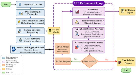
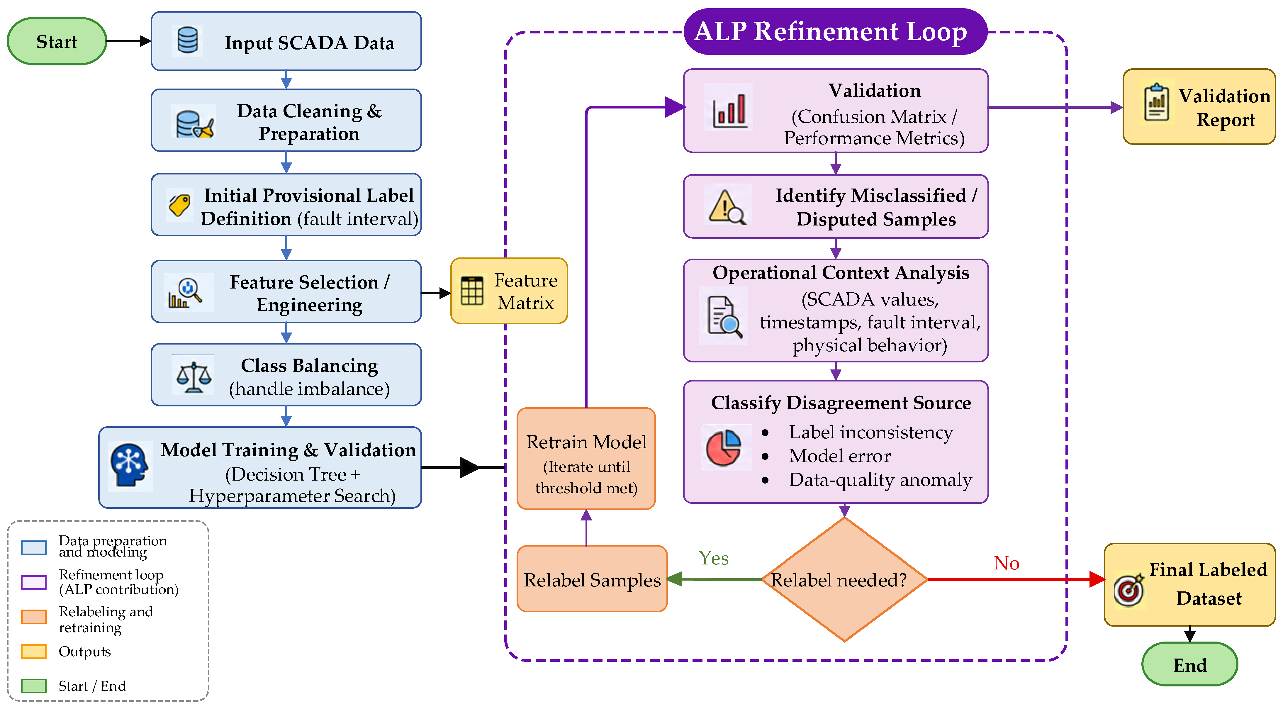
This section presents the proposed Automated Labeling Procedure (ALP) for wind turbine SCADA data. The key contribution of this work is the refinement loop applied after the identification of misclassified samples. In this loop, disagreement between the current label and the model prediction is used as an indicator of possible label inconsistency. However, these samples are not automatically relabeled. Instead, they are examined using their SCADA feature values, temporal position, relation to the fault-related reference interval, and physical consistency with wind turbine operation, and only those supported by this verification are selectively relabeled. The refined dataset is then used to retrain the model, and the process is repeated until label stability and performance convergence are achieved. The overall methodology of the procedure is illustrated in the block diagram in Figure 1.

Figure 1. Block diagram of the proposed workflow of the proposed misclassification-guided Automated Labeling Procedure (ALP) for wind turbine SCADA data.

The proposed ALP can be expressed by mapping:

$${\mathcal{D}}_{\mathrm{r}\mathrm{a}\mathrm{w}}\stackrel{\mathrm{A}\mathrm{L}\mathrm{P}}{\to }{\mathcal{D}}_{\mathrm{l}\mathrm{a}\mathrm{b}\mathrm{e}\mathrm{l}\mathrm{e}\mathrm{d}}^{*},$$

where ${\mathcal{D}}_{\mathrm{r}\mathrm{a}\mathrm{w}}$ denotes the raw SCADA dataset and ${\mathcal{D}}_{\mathrm{l}\mathrm{a}\mathrm{b}\mathrm{e}\mathrm{l}\mathrm{e}\mathrm{d}}^{*}$ denotes the final refined labeled dataset. The successive stages of the workflow are expressed as

$${\mathcal{D}}_{\mathrm{r}\mathrm{a}\mathrm{w}}\to {\mathcal{D}}_{\mathrm{p}\mathrm{r}\mathrm{e}\mathrm{p}}\to {\mathcal{D}}_{\mathrm{i}\mathrm{n}\mathrm{i}\mathrm{t}}\to {\mathcal{D}}_{\mathrm{p}\mathrm{r}\mathrm{o}\mathrm{c}}\to {\mathcal{D}}_{\mathrm{b}\mathrm{a}\mathrm{l}}\to {\mathcal{D}}_{\mathrm{m}\mathrm{o}\mathrm{d}\mathrm{e}\mathrm{l}}\to {\mathcal{D}}_{\mathrm{r}\mathrm{e}\mathrm{l}\mathrm{a}\mathrm{b}\mathrm{e}\mathrm{l}\mathrm{e}\mathrm{d}}\to {\mathcal{D}}_{\mathrm{l}\mathrm{a}\mathrm{b}\mathrm{e}\mathrm{l}\mathrm{e}\mathrm{d}}^{*}.$$

The ALP consists of the following main stages: input data description, data preparation, provisional label definition, preprocessing and feature selection, data balancing, model-based labeling, validation, misclassification analysis, relabeling, and retraining. In the proposed methodology, a DT classifier optimized by GS is used as the core classification tool within the procedure. However, the classifier is only one component of the ALP. The significance of this work lies in the development of a complete, structured, and iterative labeling workflow, with particular emphasis on the refinement loop that progressively improves label quality and dataset reliability.

2.1. Data Preparation and Initial Dataset Construction

The ALP begins with the raw SCADA dataset composed of time-series observations collected from the wind turbine system. Let the dataset be defined as

$${\mathcal{D}}_{\mathrm{r}\mathrm{a}\mathrm{w}}={\left\{\left({\mathrm{t}}_1,{\mathrm{x}}_1\right),\left({\mathrm{t}}_2,{\mathrm{x}}_2\right),\dots ,\left({\mathrm{t}}_{\mathrm{i}},{\mathrm{x}}_{\mathrm{i}}\right),\dots ,\left({\mathrm{t}}_{\mathrm{N}},{\mathrm{x}}_{\mathrm{N}}\right)\right\}}^T,$$

where $\mathrm{N}$ denotes the total number of observations, ${\mathrm{t}}_{\mathrm{i}}$ is the timestamp associated with the $\mathrm{i}$-th observation, and ${\mathrm{x}}_{\mathrm{i}}\in {\mathbb{R}}^{\mathrm{d}}$ is the corresponding $\mathrm{d}$ dimensional vector of SCADA measurements. $T$ represents the transformation of the matrix.

These variables may include measurements such as electrical power, rotor speed, generator speed, pitch angle, gearbox oil temperature, gearbox bearing temperature, nacelle temperature, and environmental parameters. However, raw SCADA data are typically affected by measurement noise, missing values, outliers, sensor degradation, and variability caused by changing operating and environmental conditions, which makes the direct interpretation of fault-related behavior difficult. SCADA variables such as temperature, speed, and torque should not be evaluated in isolation, because their values depend strongly on turbine operating state and load. Previous studies have therefore emphasized the importance of data cleaning, outlier removal, and careful preprocessing before SCADA data are used for condition monitoring and predictive modeling. Therefore, a systematic labeling and validation procedure is required before the data can be used as a reliable labeled dataset.

2.1.1. Data Preparation and Initial Label Definition

The first operational stage of the proposed ALP consists of organizing the SCADA records and defining a provisional labeling structure. The label assignment is based on the identification of a reference interval associated with abnormal, fault-related, unavailable, or maintenance-related turbine operation. In general, this reference interval may be determined by using external operational information, such as maintenance logs, alarm records, inspection reports, or operator annotations. In the supervised initialization used in this study, the ALP requires at least one reliably documented fault-related, unavailable, or maintenance-related interval to initialize the provisional labeling process. The subsequent model-based stages are then used to identify and verify potentially inconsistent labels rather than to discover faults without any prior operational reference.

Let ${\mathcal{T}}_{\mathrm{F}}$ denote the set of timestamps corresponding to this fault-related reference interval. A binary label variable ${\mathrm{y}}_{\mathrm{i}}$ is then assigned to each sample such that

$${\mathrm{y}}_{\mathrm{i}}=1\mathrm{if} {\mathrm{t}}_{\mathrm{i}}\in {\mathcal{T}}_{\mathrm{F}}, \mathrm{and} {\mathrm{y}}_{\mathrm{i}}=0\mathrm{if} {\mathrm{t}}_{\mathrm{i}}\notin {\mathcal{T}}_{\mathrm{F}}.$$

Here, ${\mathrm{y}}_{\mathrm{i}}=1$ denotes the fault-related class, whereas ${\mathrm{y}}_{\mathrm{i}}=0$ denotes the normal operating class. Accordingly, the initially labeled dataset is expressed as

$${\mathcal{D}}_{\mathrm{i}\mathrm{n}\mathrm{i}\mathrm{t}}={\left\{\left({{\mathrm{x}}_1,\mathrm{y}}_1\right),\left({\mathrm{x}}_2,{\mathrm{y}}_2\right),\dots ,\left({{\mathrm{x}}_{\mathrm{i}},\mathrm{y}}_{\mathrm{i}}\right),\dots ,\left({{\mathrm{x}}_{\mathrm{N}},\mathrm{y}}_{\mathrm{N}}\right)\right\}}^T$$

If the fault-related interval is defined by the time window $\left[{\mathrm{T}}_{\mathrm{s}},{\mathrm{T}}_{\mathrm{e}}\right]$, then the initial labels can be assigned according to

$$y_i=\left\{\begin{array}{c}1,T_s\le t_i\le T_e, \\ 0, otherwise.\end{array}\right.$$

This initial assignment provides the starting point of the ALP. At this stage, the labels are not considered final; rather, they serve as preliminary labels that are subsequently verified and refined through preprocessing, model-based classification, misclassification analysis, and relabeling. The specific definition of the reference interval used in this work is described later in the case study section.

2.1.2. Data Preprocessing and Feature Selection

After the provisional label assignment, the dataset is preprocessed to improve its quality and suitability for the ALP. This stage includes data cleaning, handling missing values, and transforming the selected variables when necessary.

To identify the most informative features, the Pearson correlation coefficient is calculated between each feature and the label variable. For the $\mathrm{j}$-th feature, the Pearson correlation coefficient is defined as

$${\mathrm{r}}_{{\mathrm{x}}_{\mathrm{j}}\mathrm{y}}={\displaystyle \frac{{\sum }_{\mathrm{i}=1}^{\mathrm{N}}({\mathrm{x}}_{\mathrm{i}\mathrm{j}}-{\overline{\mathrm{x}}}_{\mathrm{j}})({\mathrm{y}}_{\mathrm{i}}-\overline{\mathrm{y}})}{\sqrt{{\sum }_{\mathrm{i}=1}^{\mathrm{N}}{({\mathrm{x}}_{\mathrm{i}\mathrm{j}}-{\overline{\mathrm{x}}}_{\mathrm{j}})}^2}\sqrt{{\sum }_{\mathrm{i}=1}^{\mathrm{N}}{({\mathrm{y}}_{\mathrm{i}}-\overline{\mathrm{y}})}^2}}}$$

where ${\mathrm{x}}_{\mathrm{i}\mathrm{j}}$ is the value of the $\mathrm{j}$-th feature for the $\mathrm{i}$-th sample, ${\overline{\mathrm{x}}}_{\mathrm{j}}$ is the mean of the $\mathrm{j}$-th feature, and $\overline{\mathrm{y}}$ is the mean of the binary label variable. Here, ${\mathrm{y}}_{\mathrm{i}}$ is the same preliminary label previously assigned to the $\mathrm{i}$-th sample according to the fault-related reference interval. The value of ${\mathrm{r}}_{{\mathrm{x}}_{\mathrm{j}}\mathrm{y}}$ lies in the interval $\left[-\mathrm{1,1}\right]$. Features with higher absolute correlation values are considered more relevant to the labeling task. Accordingly, the selected feature subset can be expressed as

$$\mathrm{F}=\left\{{\mathrm{x}}_{\mathrm{j}}:\left|{\mathrm{r}}_{\mathrm{x}\mathrm{j}\mathrm{y}}\right|\ge \mathsf{\tau },\mathrm{j}=\mathrm{1,2},\dots ,\mathrm{m}\right\},$$

where $\mathsf{\tau }$ is the feature-selection threshold and serves as a preliminary screening parameter used to exclude variables with negligible linear association (with the preliminary labels) while retaining potentially informative SCADA features. The threshold was fixed empirically, maintaining the iterative refinement of labels.

After selecting the most relevant variables, feature scaling is performed. For each feature ${\mathrm{x}}_{\mathrm{j}}$, the standardized value ${\mathrm{z}}_{\mathrm{i}\mathrm{j}}$ is calculated as

$${\mathrm{z}}_{\mathrm{i}\mathrm{j}}={\displaystyle \frac{{\mathrm{x}}_{\mathrm{i}\mathrm{j}}-{\mathsf{\mu }}_{\mathrm{j}}}{{\mathsf{\sigma }}_{\mathrm{j}}}},$$

where ${\mathsf{\mu }}_{\mathrm{j}}$ and ${\mathsf{\sigma }}_{\mathrm{j}}$ are the mean and standard deviation of the $\mathrm{j}$-th feature, respectively.

These quantities are computed directly from the data and are therefore not selected arbitrarily. The preprocessed dataset is then represented as

$${\mathcal{D}}_{\mathrm{p}\mathrm{r}\mathrm{o}\mathrm{c}}={\left\{\left({\mathrm{z}}_1,{\mathrm{y}}_1\right),\left({\mathrm{z}}_2,{\mathrm{y}}_2\right),\dots ,\left({\mathrm{z}}_{\mathrm{i}},{\mathrm{y}}_{\mathrm{i}}\right),\dots ,\left({\mathrm{z}}_{\mathrm{N}},{\mathrm{y}}_{\mathrm{N}}\right)\right\}}^T$$

2.1.3. Data Balancing and Dataset Partitioning

Class imbalance is a common problem in industrial fault detection datasets, where normal operating samples usually dominate fault-related samples [25]. Several data-level methods have been proposed to address this issue. Classical oversampling methods, such as the Synthetic Minority Oversampling Technique (SMOTE), generate synthetic minority-class samples by interpolating between existing minority observations [26]. Improved SMOTE-based variants have also been developed, including Borderline-SMOTE, which focuses on minority samples near the class boundary [27], ADASYN, which adaptively generates more synthetic samples in difficult learning regions [28], and K-means SMOTE, which combines clustering with SMOTE to reduce noise and improve the distribution of synthetic samples [29]. More recent approaches include Deep SMOTE, which combines an encoder–decoder framework with SMOTE-based oversampling in a learned representation space [30], and feature-level oversampling methods, where synthetic samples are generated in a learned feature space rather than directly in the original input space [31].

In the present study, random undersampling was selected as a conservative balancing strategy. The main objective of the proposed ALP is not only to improve classification accuracy, but also to support label verification and iterative refinement. Therefore, preserving the physical meaning of the original SCADA observations is important. Although synthetic oversampling methods can improve minority-class representation, they may generate artificial SCADA operating points that are mathematically plausible but difficult to verify physically, especially during abnormal, unavailable, or maintenance-related turbine operation. For this reason, random undersampling was adopted in this implementation to balance the dataset while retaining only real measured SCADA records.

Let

$${\mathrm{N}}_0=\left|\left\{\mathrm{i}:{\mathrm{y}}_{\mathrm{i}}=0\right\}\right|,\hspace{1em}{\mathrm{N}}_1=\left|\left\{\mathrm{i}:{\mathrm{y}}_{\mathrm{i}}=1\right\}\right|,$$

where ${\mathrm{N}}_0$ and ${\mathrm{N}}_1$ are the numbers of normal and fault-related samples, respectively. When

$${\mathrm{N}}_0\gg {\mathrm{N}}_1,$$

the dataset is imbalanced, which may bias the classifier toward the majority class.

To reduce this effect, random undersampling is applied to the majority normal class by removing randomly selected normal samples until an approximately balanced class distribution is obtained. After balancing, the class sizes satisfy

$${\mathrm{N}}_0^{*}\approx {\mathrm{N}}_1$$

The balanced dataset is therefore written as

$${\mathcal{D}}_{\mathrm{b}\mathrm{a}\mathrm{l}}={\left\{\right({\mathrm{z}}_1,{\mathrm{y}}_1),\left({\mathrm{z}}_2,{\mathrm{y}}_2\right),\dots ,\left({\mathrm{z}}_{\mathrm{i}},{\mathrm{y}}_{\mathrm{i}}\right),\dots ,\left({\mathrm{z}}_{{\mathrm{N}}_B},{\mathrm{y}}_{{\mathrm{N}}_B}\right)\}}^T$$

where ${\mathrm{N}}_{\mathrm{B}}$ is the total number of samples after balancing.

For model development, the balanced dataset is partitioned into training, validation, and test subsets such that

$${\mathcal{D}}_{\mathrm{b}\mathrm{a}\mathrm{l}}={\mathcal{D}}_{\mathrm{t}\mathrm{r}\mathrm{a}\mathrm{i}\mathrm{n}}\cup {\mathcal{D}}_{\mathrm{v}\mathrm{a}\mathrm{l}}\cup {\mathcal{D}}_{\mathrm{t}\mathrm{e}\mathrm{s}\mathrm{t}}$$

with

$${\mathcal{D}}_{\mathrm{t}\mathrm{r}\mathrm{a}\mathrm{i}\mathrm{n}}\cap {\mathcal{D}}_{\mathrm{v}\mathrm{a}\mathrm{l}}\cap {\mathcal{D}}_{\mathrm{t}\mathrm{e}\mathrm{s}\mathrm{t}}=\mathrm{\varnothing }$$

In the proposed framework, the split ratio is defined as 60% for training, 20% for validation, and 20% for testing, which gives

$$\left|{\mathcal{D}}_{\mathrm{t}\mathrm{r}\mathrm{a}\mathrm{i}\mathrm{n}}\right|=0.6{\mathrm{N}}_{\mathrm{B}},\left|{\mathcal{D}}_{\mathrm{v}\mathrm{a}\mathrm{l}}\right|=0.2{\mathrm{N}}_{\mathrm{B}},\left|{\mathcal{D}}_{\mathrm{t}\mathrm{e}\mathrm{s}\mathrm{t}}\right|=0.2{\mathrm{N}}_{\mathrm{B}}.$$

2.2. Model-Based Labeling

After data preparation, preprocessing, and balancing, the next stage of the proposed ALP is model-based labeling. In the considered case study, a Decision Tree (DT) classifier is employed as the core model for assigning labels to SCADA data. To improve its generalization ability and reduce overfitting, the DT model is optimized using the Grid Search (GS) algorithm.

2.2.1. DT Classifier

A DT is a supervised machine-learning model used to solve classification and regression problems [32,33,34,35]. In the proposed Automated Labeling Procedure (ALP), the DT is employed for binary classification of SCADA samples into two classes: Normal and Fault. Its main advantage lies in its interpretability, since the classification process can be represented as a hierarchical sequence of decision rules based on SCADA variables.

Let the input sample be represented by the feature vector

$${\mathrm{z}}_{\mathrm{i}}=[{\mathrm{z}}_{\mathrm{i}1},{\mathrm{z}}_{\mathrm{i}2},\dots ,{\mathrm{z}}_{\mathrm{i}\mathrm{p}}{]}^{\mathrm{T}}\in {\mathbb{R}}^{\mathrm{p}},$$

where $\mathrm{p}$ is the number of selected SCADA features and ${\mathrm{z}}_{\mathrm{i}\mathrm{j}}$ is the value of the $\mathrm{j}$-th feature for the $\mathrm{i}$-th sample. The components of ${\mathrm{z}}_{\mathrm{i}}$ correspond to operational and condition monitoring variables measured by the wind turbine SCADA system, such as active power output, wind speed, rotor speed, generator speed, gearbox oil temperature, bearing temperatures, and other signals describing turbine and gearbox behavior. The DT classifier can then be written as

$${\widehat{\mathrm{y}}}_{\mathrm{i}}=\mathrm{f}\left({\mathrm{z}}_{\mathrm{i}};\mathsf{\theta }\right),$$

where ${\widehat{\mathrm{y}}}_{\mathrm{i}}\in \left\{\mathrm{0,1}\right\}$ is the predicted label, $\mathrm{f}(\cdot )$ denotes the tree-based decision function, and $\mathsf{\theta }$ is the set of model hyperparameters.

Each internal node applies a threshold condition of the form

$${\mathrm{z}}_{\mathrm{i}\mathrm{j}}\le {\mathsf{\tau }}_{\mathrm{n}},$$

where ${\mathrm{z}}_{\mathrm{i}\mathrm{j}}$ is the selected feature and ${\mathsf{\tau }}_{\mathrm{n}}$ is the split threshold automatically determined during training. By recursively applying such rules, the classifier assigns each sample to either the Normal or Fault class.

The quality of each split is evaluated using a Gini impurity criterion. In the implemented approach, the Gini impurity is used and is defined as

$$\mathrm{G}(\mathrm{n})=1-{\displaystyle \sum _{\mathrm{c}=1}^{\mathrm{C}}}{\mathrm{p}}_{\mathrm{c}}^2,$$

where ${\mathrm{p}}_{\mathrm{c}}$ is the proportion of samples belonging to class $\mathrm{c}$ at node $\mathrm{n}$, and $\mathrm{C}$ is the number of classes. For the binary case considered in this study,

$$\mathrm{G}\left(\mathrm{n}\right)=1-({\mathrm{p}}_0^2+{\mathrm{p}}_1^2),$$

where ${\mathrm{p}}_0$ and ${\mathrm{p}}_1$ denote the proportions of Normal and Fault samples, respectively. The optimal split is selected by maximizing the impurity reduction:

$$\mathsf{\Delta }\mathrm{G}=\mathrm{G}(\mathrm{n})-\left({\displaystyle \frac{{\mathrm{N}}_{\mathrm{l}\mathrm{e}\mathrm{f}\mathrm{t}}}{{\mathrm{N}}_{\mathrm{n}}}}\mathrm{G}({\mathrm{n}}_{\mathrm{l}\mathrm{e}\mathrm{f}\mathrm{t}})+{\displaystyle \frac{{\mathrm{N}}_{\mathrm{r}\mathrm{i}\mathrm{g}\mathrm{h}\mathrm{t}}}{{\mathrm{N}}_{\mathrm{n}}}}\mathrm{G}({\mathrm{n}}_{\mathrm{r}\mathrm{i}\mathrm{g}\mathrm{h}\mathrm{t}})\right),$$

where ${\mathrm{N}}_{\mathrm{n}}$ is the number of samples at node $\mathrm{n}$, and ${\mathrm{N}}_{\mathrm{l}\mathrm{e}\mathrm{f}\mathrm{t}}$ and ${\mathrm{N}}_{\mathrm{r}\mathrm{i}\mathrm{g}\mathrm{h}\mathrm{t}}$ are the numbers of samples assigned to the left and right child nodes, respectively.

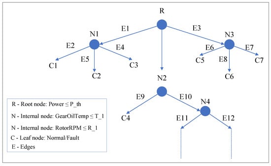
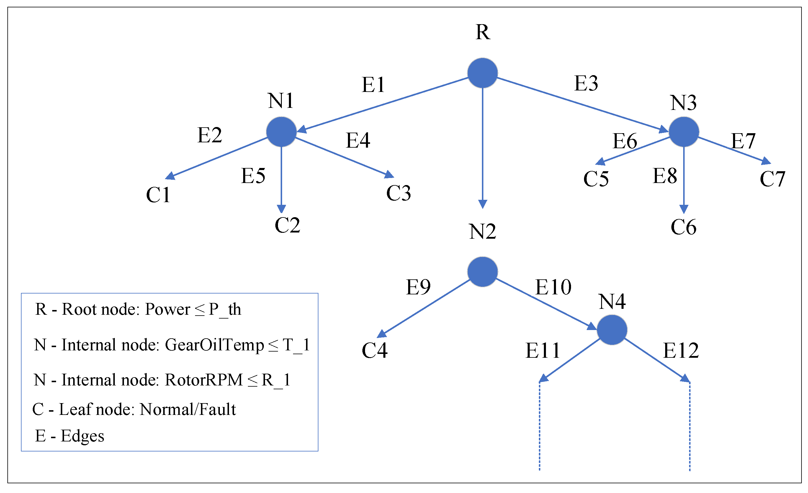
Figure 2 illustrates an example of the DT structure obtained for SCADA-based classification. In this example, the root node performs a first split using turbine power, which separates operating conditions according to a power threshold. Subsequent internal nodes apply additional rules based on variables such as gearbox oil temperature and rotor speed. The leaf nodes then assign the final class label, Normal or Fault. This example highlights the main reason for selecting DT as the core validation model in the ALP: beyond its predictive performance, it provides a transparent rule-based structure that allows the labeling decisions to be inspected and interpreted in terms of physically meaningful SCADA variables.

Figure 2. Illustrative structure of a DT classifier using representative SCADA parameters. Dashed lines indicate that the decision tree continues beyond the branches displayed.

2.2.2. Grid Search Optimization

Although DTs are effective and interpretable classifiers, their performance depends strongly on the choice of hyperparameters [36]. Parameters controlling the depth of the tree and the minimum number of samples required for splitting and leaf creation have a direct influence on model complexity, generalization ability, and susceptibility to overfitting. For this reason, Grid Search (GS) is employed in the proposed ALP to determine the most suitable hyperparameter configuration for the DT model [37,38].

GS is a systematic hyperparameter optimization technique that evaluates all possible combinations from a predefined set of candidate values. Let the DT hyperparameter vector be defined as

$$\mathsf{\theta }=\left[\mathrm{max\_depth}, \mathrm{min\_samples\_split}, \mathrm{min\_samples\_leaf}\right],$$

The corresponding hyperparameter search space is expressed as

$$\mathsf{\Theta }={\mathsf{\Theta }}_1\times {\mathsf{\Theta }}_2\times {\mathsf{\Theta }}_3,$$

where each set ${\mathsf{\Theta }}_{\mathrm{k}}$ contains the candidate values of the $\mathrm{k}$-th hyperparameter. GS then evaluates all combinations

$${\mathsf{\theta }}^{\left(\mathrm{q}\right)}\in \mathsf{\Theta },\mathrm{q}=\mathrm{1,2},\dots ,\mathrm{Q},$$

where $\mathrm{Q}$ denotes the total number of tested hyperparameter combinations.

For each candidate combination ${\mathsf{\theta }}^{\left(\mathrm{q}\right)}$, a DT model is trained and evaluated by cross-validation. Let ${\mathrm{K}}_{\mathrm{f}}$ denote the number of folds and let ${\mathrm{S}}_{\mathrm{k}}\left({\mathsf{\theta }}^{\left(\mathrm{q}\right)}\right)$ denote the validation score obtained for the $\mathrm{k}$-th fold. The mean cross-validation score is then computed as

$$\mathrm{J}\left({\mathsf{\theta }}^{\left(\mathrm{q}\right)}\right)={\displaystyle \frac{1}{{\mathrm{K}}_{\mathrm{f}}}}{\displaystyle \sum _{\mathrm{k}=1}^{{\mathrm{K}}_{\mathrm{f}}}}{\mathrm{S}}_{\mathrm{k}}\left({\mathsf{\theta }}^{\left(\mathrm{q}\right)}\right).$$

The optimal hyperparameter vector is selected as the one that maximizes the average validation score:

$${\mathsf{\theta }}^{*}=\mathrm{a}\mathrm{r}\mathrm{g}\underset{{\mathsf{\theta }}^{\left(\mathrm{q}\right)}\in \mathsf{\Theta }}{\mathrm{m}\mathrm{a}\mathrm{x}}\mathrm{J}\left({\mathsf{\theta }}^{\left(\mathrm{q}\right)}\right).$$

Consequently, the final optimized DT classifier used in the ALP is written as

$${\widehat{\mathrm{y}}}_{\mathrm{i}}=\mathrm{f}({\mathrm{z}}_{\mathrm{i}};{\mathsf{\theta }}^{*}),$$

where ${\mathrm{z}}_{\mathrm{i}}$ is the input feature vector of sample $\mathrm{i}$, $\mathrm{f}(\cdot )$ is the DT decision function, and ${\widehat{\mathrm{y}}}_{\mathrm{i}}$ is the predicted label.

2.2.3. Role of the Optimized Classifier Within the ALP

Within the proposed ALP, the DT optimized by GS serves as the classification engine used to generate prediction outputs from the prepared SCADA dataset. However, it should be emphasized that this optimized classifier is only one component of the overall framework.

More specifically, the optimized classifier produces the predicted labels that are subsequently compared with the provisional labels during the validation stage. The resulting disagreements are used to identify potentially inconsistent samples, which are then examined in the refinement loop of the ALP. In this way, the DT–GS combination supports the verification and correction of preliminary labels and contributes to the progressive improvement of dataset consistency.

2.3. Critical Step of the ALP: The Iterative Refinement Loop

The critical methodological component of the proposed ALP is the iterative refinement loop. Rather than treating the assigned labels as fixed, the proposed ALP progressively verifies and refines them. After the initial model-based validation stage, the classifier outputs are compared with the current labels to identify potentially inconsistent observations. These samples are then examined through misclassification analysis, selectively relabeled when justified, and reintroduced into the dataset for model retraining. In this way, the ALP uses model feedback not only for prediction, but also for progressive improvement of dataset quality. The process is repeated until the label set becomes stable and no further meaningful improvement is observed.

2.3.1. Validation and Performance Evaluation

After the DT classifier has been optimized and trained, its predictions are evaluated on the validation subset to assess the consistency between the model output and the current labels. Let the validation dataset be denoted by

$${\mathcal{D}}_{\mathrm{v}\mathrm{a}\mathrm{l}}={\left\{\right({\mathrm{z}}_1,{\mathrm{y}}_1),\left({\mathrm{z}}_2,{\mathrm{y}}_2\right),\dots ,\left({\mathrm{z}}_{\mathrm{i}},{\mathrm{y}}_{\mathrm{i}}\right),\dots ,\left({\mathrm{z}}_{{\mathrm{N}}_{val}},{\mathrm{y}}_{{\mathrm{N}}_{val}}\right)\}}^T,$$

where ${\mathrm{z}}_i$ is the preprocessed feature vector, $y_i\in \left\{\mathrm{0,1}\right\}$ is the current label, and ${\mathrm{N}}_{\mathrm{v}\mathrm{a}\mathrm{l}}$ is the number of validation samples. For each sample, the classifier produces a predicted label

$${\widehat{\mathrm{y}}}_{\mathrm{i}}=\mathrm{f}({\mathrm{z}}_{\mathrm{i}};{\mathsf{\theta }}^{*}),$$

where ${\mathsf{\theta }}^{*}$ is the optimal hyperparameter configuration selected during Grid Search.

The validation performance is quantified using the confusion matrix and the corresponding classification metrics. Let $\mathrm{T}\mathrm{P}$, $\mathrm{T}\mathrm{N}$, $\mathrm{F}\mathrm{P}$, and $\mathrm{F}\mathrm{N}$ denote the numbers of true positives, true negatives, false positives, and false negatives, respectively. The evaluation measures are defined as follows:

$$\mathrm{A}\mathrm{c}\mathrm{c}\mathrm{u}\mathrm{r}\mathrm{a}\mathrm{c}\mathrm{y}={\displaystyle \frac{\mathrm{T}\mathrm{P}+\mathrm{T}\mathrm{N}}{\mathrm{T}\mathrm{P}+\mathrm{T}\mathrm{N}+\mathrm{F}\mathrm{P}+\mathrm{F}\mathrm{N}}}$$

$${\mathrm{F}}_1={\displaystyle \frac{2\mathrm{T}\mathrm{P}}{2\mathrm{T}\mathrm{P}+\mathrm{F}\mathrm{P}+\mathrm{F}\mathrm{N}}}$$

$$\mathrm{I}\mathrm{o}\mathrm{U}={\displaystyle \frac{\mathrm{T}\mathrm{P}}{\mathrm{T}\mathrm{P}+\mathrm{F}\mathrm{P}+\mathrm{F}\mathrm{N}}}$$

These metrics provide a quantitative assessment of the model-based labeling stage. However, within the proposed ALP, their role is not limited to measuring classifier performance. They also serve as indicators of the quality and consistency of the current label set. Samples associated with incorrect predictions become candidates for further analysis in the refinement loop.

2.3.2. Misclassification Analysis

This stage represents the starting point of the main ALP contribution, because the detected misclassifications are used not only to evaluate classifier performance, but also to trigger the label refinement mechanism.

Once the validation results are obtained, the next step of the ALP consists of identifying and analyzing the samples for which the predicted labels disagree with the current labels. At iteration $\mathrm{t}$, the set of misclassified samples is defined as

$${\mathcal{M}}^{\left(\mathrm{t}\right)}=\left\{\mathrm{i}\hspace{0.25em}\mid \hspace{0.25em}{\widehat{\mathrm{y}}}_{\mathrm{i}}^{\left(\mathrm{t}\right)}≠{\mathrm{y}}_{\mathrm{i}}^{\left(\mathrm{t}\right)}\right\},$$

where ${\mathrm{y}}_{\mathrm{i}}^{\left(\mathrm{t}\right)}$ denotes the current label of sample $\mathrm{i}$, and ${\widehat{\mathrm{y}}}_{\mathrm{i}}^{\left(\mathrm{t}\right)}$ denotes the label predicted by the classifier at iteration $\mathrm{t}$.

The elements of ${\mathcal{M}}^{\left(\mathrm{t}\right)}$ are treated as suspicious samples, since the disagreement may arise from two possible sources: either the classifier fails to generalize correctly, or the provisional assignment is not fully consistent with the actual SCADA behavior. In the proposed ALP, these misclassified observations are not automatically considered as labeling errors. Instead, they are examined as potentially ambiguous or unreliable samples requiring further verification.

The misclassification analysis is performed by examining the operational context of the disputed observations. In the case of wind turbine SCADA data, this analysis may involve the inspection of the corresponding SCADA variables, their local temporal behavior, and their relation to known operational or fault-related intervals. Samples located near class boundaries, transition periods, or noisy operating conditions are particularly important, since such records are more likely to contain uncertain or inconsistent labels.

Therefore, the purpose of this stage is to transform raw disagreement information into informed relabeling candidates. In this sense, misclassification analysis acts as the diagnostic bridge between classifier output and label correction and constitutes a central part of the ALP refinement logic.

2.3.3. Relabeling Strategy

After the misclassified samples have been identified and analyzed, a selective relabeling strategy is applied. The key principle of the proposed ALP is that relabeling is performed only for samples whose inconsistency is considered justified after the analysis stage. Let

$${\mathcal{R}}^{\left(\mathrm{t}\right)}\subseteq {\mathcal{M}}^{\left(\mathrm{t}\right)}$$

denote the subset of samples selected for relabeling at iteration $\mathrm{t}$. These are the observations for which the model prediction is considered more reliable than the current assigned label, based on the validation evidence and the misclassification analysis.

The label update rule is then defined as

$${\mathrm{y}}_{\mathrm{i}}^{\left(\mathrm{t}+1\right)}=\left\{\begin{array}{cc}{\widehat{\mathrm{y}}}_{\mathrm{i}}^{\left(\mathrm{t}\right)},& \mathrm{i}\in {\mathcal{R}}^{\left(\mathrm{t}\right)}\\ {\mathrm{y}}_{\mathrm{i}}^{\left(\mathrm{t}\right)},& \mathrm{i}\notin {\mathcal{R}}^{\left(\mathrm{t}\right)}\end{array}\right.$$

where ${\mathrm{y}}_{\mathrm{i}}^{\left(\mathrm{t}+1\right)}$ is the updated label after iteration $\mathrm{t}$. Accordingly, only the validated suspicious samples are reassigned, while the remaining observations preserve their current labels.

The relabeled dataset obtained at iteration $\mathrm{t}+1$ is written as

$${\mathcal{D}}_{\mathrm{r}\mathrm{e}\mathrm{l}\mathrm{a}\mathrm{b}\mathrm{e}\mathrm{l}\mathrm{e}\mathrm{d}}^{\left(\mathrm{t}+1\right)}={\left\{({\mathrm{z}}_1,{\mathrm{y}}_1^{\left(\mathrm{t}+1\right)}),({\mathrm{z}}_2,{\mathrm{y}}_2^{\left(\mathrm{t}+1\right)}),\dots ,({\mathrm{z}}_{\mathrm{i}},{\mathrm{y}}_{\mathrm{i}}^{\left(\mathrm{t}+1\right)}),\dots ,({\mathrm{z}}_{{\mathrm{N}}_B},{\mathrm{y}}_{{\mathrm{N}}_B}^{\left(\mathrm{t}+1\right)})\right\}}^T$$

where ${\mathrm{N}}_{\mathrm{B}}$ is the size of the balanced dataset used in the study.

This selective strategy is essential for preserving the interpretability and robustness of the ALP. It prevents unjustified relabeling of difficult but correctly labeled samples, and ensures that the refinement process remains controlled rather than arbitrary. Therefore, the proposed relabeling strategy is not a simple replacement of labels by predictions; rather, it is a validation-guided correction mechanism embedded within the iterative workflow.

2.3.4. Model Retraining and Convergence Criterion

After the dataset has been updated through selective relabeling, the classifier is retrained using the refined label set. At iteration $\mathrm{t}+1$, the updated model is expressed as

$${\widehat{\mathrm{y}}}_{\mathrm{i}}^{\left(\mathrm{t}+1\right)}=\mathrm{f}({\mathrm{z}}_{\mathrm{i}};{\mathsf{\theta }}^{*(\mathrm{t}+1)}),$$

where ${\mathsf{\theta }}^{*(\mathrm{t}+1)}$ denotes the optimized model parameters obtained after retraining on the refined dataset. The new model is then evaluated again on the validation subset, and the same cycle of validation, misclassification analysis, and selective relabeling is repeated.

This iterative procedure continues until a convergence condition is satisfied. In the proposed ALP, convergence is defined by the absence of additional justified relabeling and by negligible improvement in F1-score between successive iterations.

A performance-based criterion can be written as

$$\mid {\mathrm{F}}_1^{\left(\mathrm{t}+1\right)}-{\mathrm{F}}_1^{\left(\mathrm{t}\right)}\mid <\mathsf{\epsilon },$$

where $\mathsf{\epsilon }$ is a predefined tolerance. In parallel, a label stability condition may be defined as

$$\mid {\mathcal{R}}^{\left(\mathrm{t}\right)}\mid =0,$$

which indicates that no additional samples have been selected for justified relabeling at iteration $\mathrm{t}$.

Accordingly, the refinement loop is terminated when the label set becomes stable, and the classifier’s performance no longer shows meaningful improvement. The output of this stage is the final refined labeled dataset,

$${\mathcal{D}}_{\mathrm{l}\mathrm{a}\mathrm{b}\mathrm{e}\mathrm{l}\mathrm{e}\mathrm{d}}^{*},$$

which constitutes the product of the proposed ALP and serves as the basis for the subsequent case-study analysis.

2.3.5. Final Output of the ALP

The final output of the proposed ALP is a refined labeled dataset, denoted by

$${\mathcal{D}}_{\mathrm{l}\mathrm{a}\mathrm{b}\mathrm{e}\mathrm{l}\mathrm{e}\mathrm{d}}^{*},$$

which is obtained after the successive stages of data preparation, provisional label assignment, preprocessing, feature selection, balancing, model-based labeling, validation, misclassification analysis, selective relabeling, and model retraining.

Accordingly, the ALP can be understood as a complete mapping from the raw SCADA dataset to the final validated dataset:

$${\mathcal{D}}_{\mathrm{r}\mathrm{a}\mathrm{w}}\stackrel{\mathrm{A}\mathrm{L}\mathrm{P}}{\to }{\mathcal{D}}_{\mathrm{l}\mathrm{a}\mathrm{b}\mathrm{e}\mathrm{l}\mathrm{e}\mathrm{d}}^{*}.$$

The importance of this final output lies in the fact that it is not generated by a single classification step, but by a structured and interpretable workflow in which provisional labels are progressively verified and corrected.

The general ALP presented in this section is confirmed in the following section with a wind turbine SCADA case study.

2.4. Computational Complexity and Overfitting Control

Let (N) denote the number of SCADA observations, (p) the number of selected features, (K) the number of Grid Search combinations, (C) the number of cross-validation folds, (d) the Decision Tree depth, and (R) the number of refinement iterations. The overall computational complexity is approximately

$$\mathrm{O}\left(\mathrm{R}\right(\mathrm{K}\mathrm{C}\mathrm{N}\mathrm{p}\mathrm{l}\mathrm{o}\mathrm{g}\mathrm{N}+\mathrm{N}\mathrm{d}\left)\right)$$

In practice, the number of refinement iterations remains small, and only disputed samples require detailed verification.

The risk of overfitting is controlled using mutually exclusive training, validation, and test subsets, five-fold cross-validation, tree-complexity parameters, cost-complexity pruning, and learning-curve analysis. Generalization is assessed using validation and test performance rather than training accuracy alone. The final relabeled dataset is also evaluated using Random Forest, XGBoost, and Gradient Boosting.

3. Case Study: Application of the ALP to Wind Turbine SCADA Data

The individual stages of the procedure are implemented on real operational data, and the effectiveness of the refined labeling strategy is evaluated through quantitative performance metrics and comparative analysis. The case study describes the implementation of each stage of the ALP, from raw data preparation and provisional label assignment to preprocessing, balancing, and model-based labeling. The purpose of the case study is to show how the proposed procedure can generate a refined labeled dataset from previously unlabeled SCADA records, thereby providing a reliable basis for subsequent fault detection analysis.

3.1. SCADA Dataset

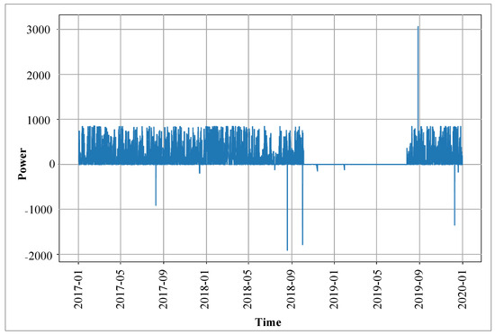
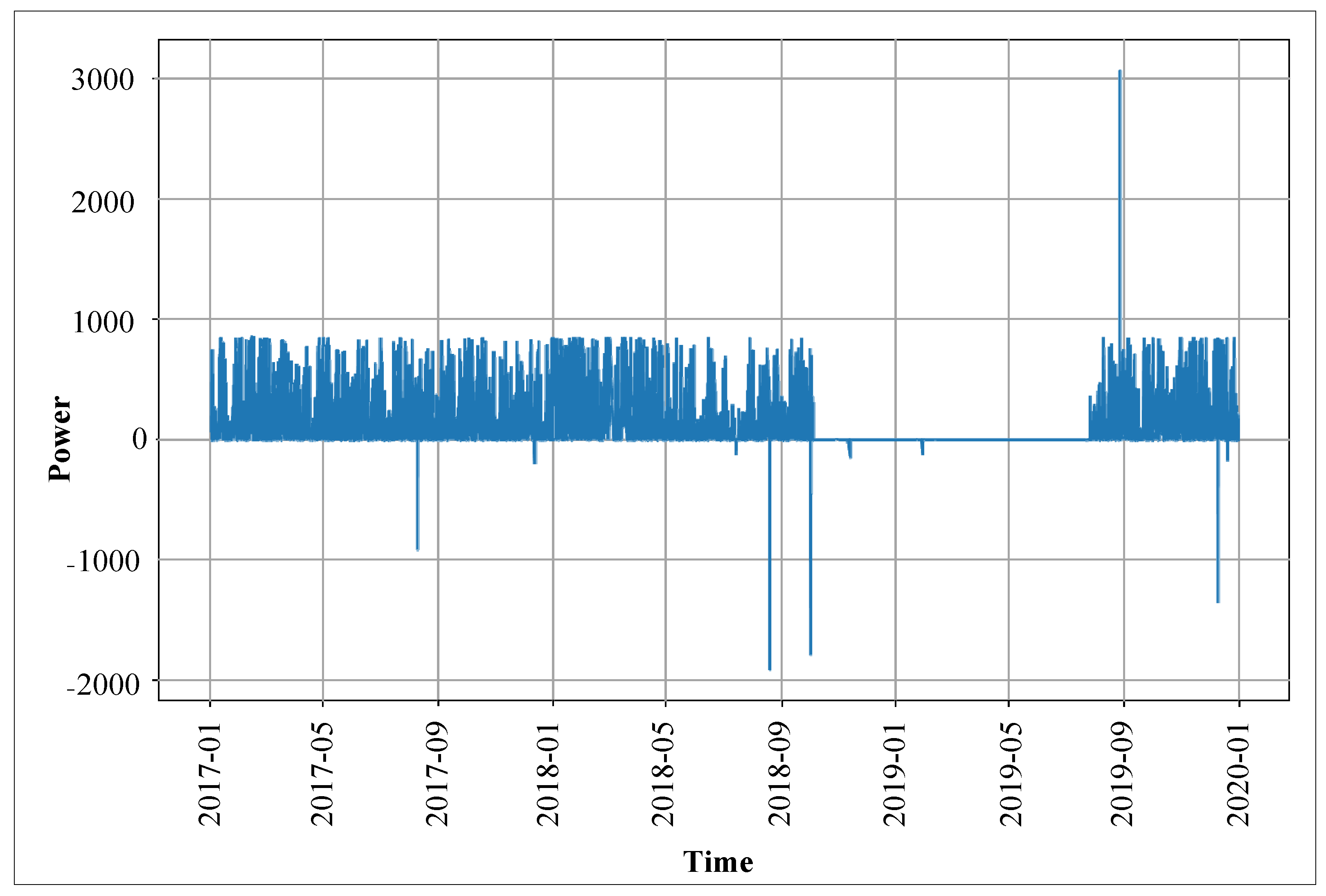
The case study considered in this manuscript is based on multi-annual 10 min raw SCADA data collected from a wind turbine located in Ireland. The dataset covers the period from 1 January 2017 to 31 December 2019 and describes the operational behavior of the turbine over a long-term monitoring interval [39].

The wind turbine has a hub height of 60 m and a rotor diameter of 52 m. During the observation period, a major gearbox changeout took place between 4 October 2018 and 27 July 2019. Throughout this interval, no positive electrical power output was recorded. This event provides a meaningful operational reference for the present study, since it corresponds to an abnormal or unavailable turbine state associated with maintenance activity.

The SCADA records include a wide range of operational and environmental variables, such as active power, rotor speed, generator speed, pitch angle, gearbox oil temperature, gearbox bearing temperature, generator temperatures, nacelle temperature, and ambient conditions. Owing to its long time span and the presence of a clearly identified abnormal operational interval, this dataset is well suited for evaluating the proposed ALP in a realistic wind energy context.

3.2. Case-Specific Provisional Label Definition

The original SCADA dataset was unlabeled. To initialize the ALP, a binary label variable was introduced using the gearbox-changeout interval as a fault-related reference period. More specifically, the records corresponding to the gearbox-changeout interval were initially assigned to the Fault class, whereas the remaining records were assigned to the Normal class. This documented event provides the operational reference required to initialize the provisional labels used by the ALP.

Let ${\mathrm{t}}_{\mathrm{i}}$ denote the timestamp of the $\mathrm{i}$-th SCADA observation and let $\left[{\mathrm{T}}_{\mathrm{s}},{\mathrm{T}}_{\mathrm{e}}\right]$ denote the time interval associated with the gearbox changeout. The initial label is then defined as

$${\mathrm{y}}_{\mathrm{i}}=\left\{\begin{array}{cc}1,& {\mathrm{T}}_{\mathrm{s}}\le {\mathrm{t}}_{\mathrm{i}}\le {\mathrm{T}}_{\mathrm{e}}\\ 0,& \mathrm{otherwise}\end{array}\right.$$

where ${\mathrm{y}}_{\mathrm{i}}=1$ denotes a fault-related sample and ${\mathrm{y}}_{\mathrm{i}}=0$ denotes a normal-operation sample. Figure 3 presents the active power time series and highlights the interval used to define the initial labels.

Figure 3. Active power output of the wind turbine over the study period, highlighting the gearbox-changeout interval used for the initial label definition.

3.3. Case Study Data Preprocessing and Feature Selection

After the provisional labels were assigned, the dataset was preprocessed to improve its suitability for the ALP workflow. This stage included the organization of the SCADA records, treatment of incomplete or inconsistent observations, and preparation of the variables used in the subsequent model-based labeling stage.

To identify the informative variables for distinguishing between normal and fault-related operating states, the Pearson correlation coefficient was computed between each candidate feature and the binary label variable, with a fixed threshold coefficient defined as a moderate screening criterion. This value is chosen to remove variables with negligible correlation while preserving weakly but potentially meaningful features, which is consistent with the objective of the proposed ALP. Features with higher absolute correlation values were considered more relevant for the classification task and were therefore retained for further analysis. The selected feature subset is reported in Table 1.

Table 1. Selected SCADA features used for fault-related labeling.

Feature Title	Description	Correlation with Label (Absolute Value)
Fault Label	Fault label (normal and fault data)	1
Pitch	Pitch angle	0.7–0.8
GearBearTemp	Gearbox bearing temperature (°C)	0.85–0.92
GearOilTemp	Gearbox oil temperature (°C)	0.78–0.85
GenBearTemp	Generator bearing temperature (°C)	0.68–0.78
RotorRPM	Wind turbine rotor revs per minute (RPM)	0.94–0.97
GenRPM	Electrical generator revs per minute (RPM)	0.95–0.98
GenPh1Temp	Generator phase 1 winding temperature (°C)	0.81–0.89
GenPh2Temp	Generator phase 2 winding temperature (°C)	0.81–0.89
GenPh3Temp	Generator phase 3 winding temperature (°C)	0.82–0.9
NacelTemp	Temperature inside nacelle space (°C)	0.4–0.55
MaxPower	Maximum 10 min power output (kW)	0.6–0.72
StdDevPower	Wind speed standard deviation (m/s) in 10 min period	0.55–0.68
Power	Average 10 min power output (kW)	0.52–0.65
MinPower	Minimum 10 min power output (kW)	0.48–0.6
AvgRPow	Average 10 min reactive power output (kVAR)	0.5–0.62

The selected variables mainly describe turbine production, drivetrain behavior, and thermal operating conditions, all of which are expected to be influenced by gearbox-related abnormal operations.

After feature selection, the retained numerical variables were standardized to ensure a consistent representation across the evaluated classifiers.

3.4. Data Balancing and Experimental Setup

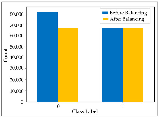
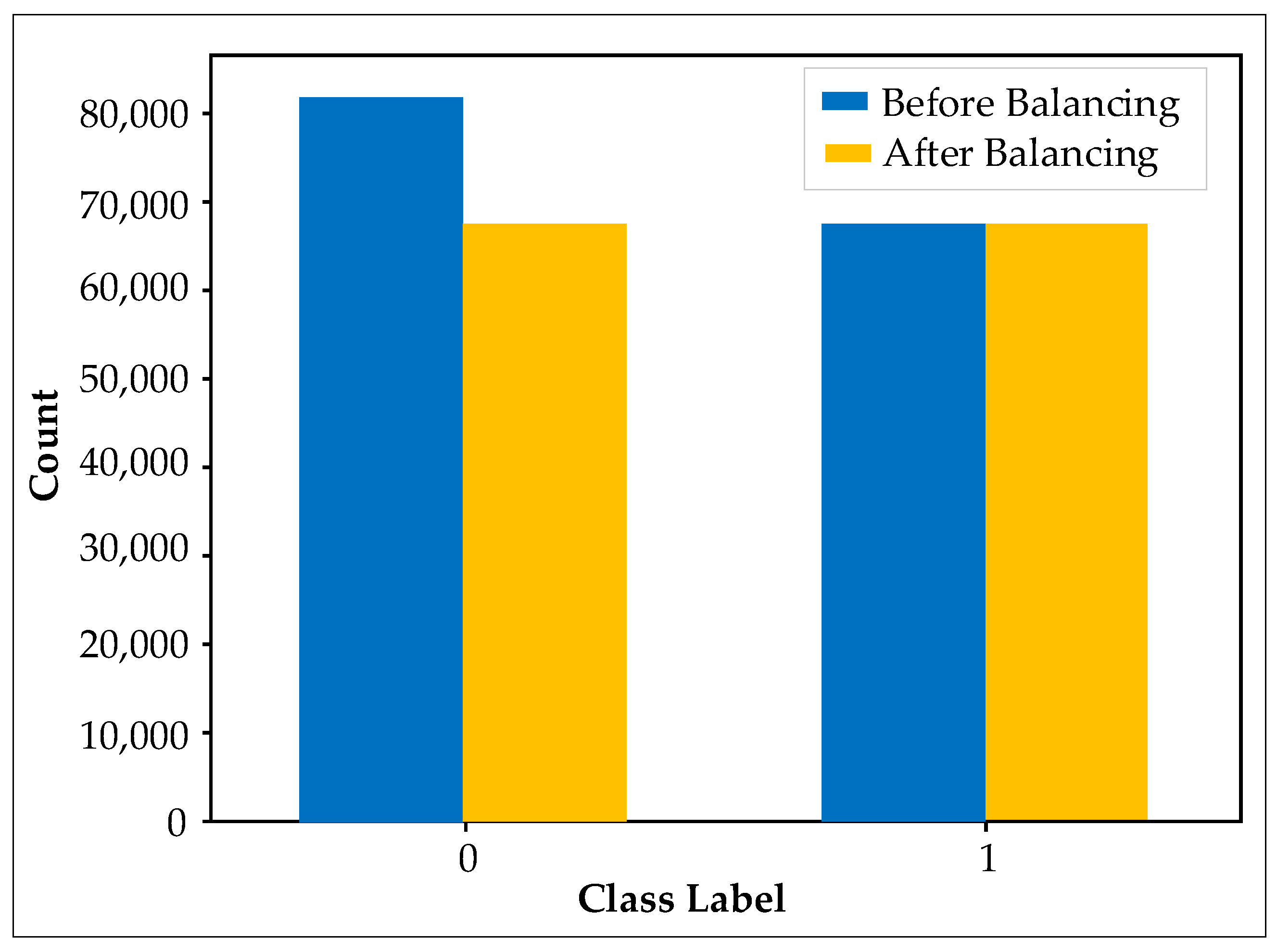
The initially labeled dataset exhibited a marked class imbalance, with normal-operation samples significantly outnumbering fault-related samples. Specifically, the dataset contained 82,466 healthy samples, exceeding the number of fault samples by 14,350. Such imbalance can reduce the sensitivity of machine-learning models to the minority class and bias the classification outcome toward normal operation.

To alleviate this effect, a random undersampling strategy was applied to the majority class, by randomly removing 14,350 healthy samples. The distribution of samples before and after balancing is illustrated in Figure 4, where labels 0 and 1 represent normal and faulty samples, respectively.

Figure 4. Class distribution before and after random undersampling of the healthy class.

3.5. Classification of the Prelabeled Data

The classification stage of the ALP was first implemented using a baseline DT classifier. This model was selected because of its interpretability and its suitability for both classification and the examination of potentially inconsistent labels. At each internal node, the split threshold was determined during training.

The initial DT model achieved very high training performance, but the discrepancy between training and validation/test behavior suggested the presence of overfitting. For this reason, GS optimization was applied to identify a more suitable hyperparameter configuration. The optimization process focused on the main complexity controlling parameters of the tree, namely max_depth, min_samples_split, and min_samples_leaf, as defined in Section 2.

The optimized DT was then used as the core classification model within the ALP. During validation, its predictions were compared with the current dataset labels to identify disagreements and potentially suspicious observations. These samples were subsequently used in the iterative refinement loop, where misclassification analysis and selective relabeling were performed to improve label consistency.

The classifier provides predictions that help the ALP identify potentially unreliable labels and progressively improve dataset quality.

The quantitative performance of the baseline and optimized models, together with the comparison against alternative classifiers and the effect of the iterative relabeling process, are presented in the next section.

4. Results, Comparative Analysis and Discussion

Since the main contribution of the proposed ALP is the refinement loop rather than the classifier alone, the results are analyzed from two perspectives: first, the predictive performance of the classifiers, and second, the ability of the ALP to identify, interpret, and selectively correct inconsistent labels.

The results are organized in four stages. First, the performance of the baseline DT and the optimized GS-DT is compared to evaluate the effect of hyperparameter tuning. Second, the optimized DT is compared with two additional classifiers, namely Random Forest (RF) and XGBoost (XGB), using standard performance metrics. Third, the model disagreements are examined through misclassification analysis to identify potentially inconsistent labels. Finally, the effect of the iterative relabeling stage is assessed by repeating the workflow on the refined dataset and comparing the resulting classification performance. In this way, this section evaluates not only the predictive capability of individual models, but also the effectiveness of the ALP as a complete labeling framework.

4.1. Performance Before and After DT Optimization

A baseline DT model was first trained using the prepared SCADA dataset. Although this initial model achieved a high training accuracy, presented in Table 2, its test performance was substantially lower, indicating that the classifier had learned the training data too closely and did not generalize well to unseen samples. This behavior is characteristic of overfitting.

Table 2. Performance of the baseline DT and the Grid Search-optimized DT.

Model	Accuracy	Precision	Recall	F1-Score
DT	88.02%	88.02%	88.01%	88.02%
GS-DT	99.985%	99.993%	99.978%	99.985%

As shown in Table 2, the baseline DT achieved an accuracy of 88.02%, with precision, recall, and F1-score all close to 88%. These results indicate that the untuned DT, despite fitting the training data extremely well, was not sufficiently robust when applied to unseen observations.

To mitigate this issue, GS optimization was applied to tune the main hyperparameters controlling tree complexity, namely max_depth, min_samples_split, and min_samples_leaf. After optimization, the performance of the DT improved markedly. The optimized GS-DT reached an accuracy of 99.985%, with equally high precision, recall, and F1-score, demonstrating a substantial gain in predictive reliability.

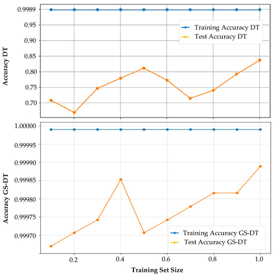
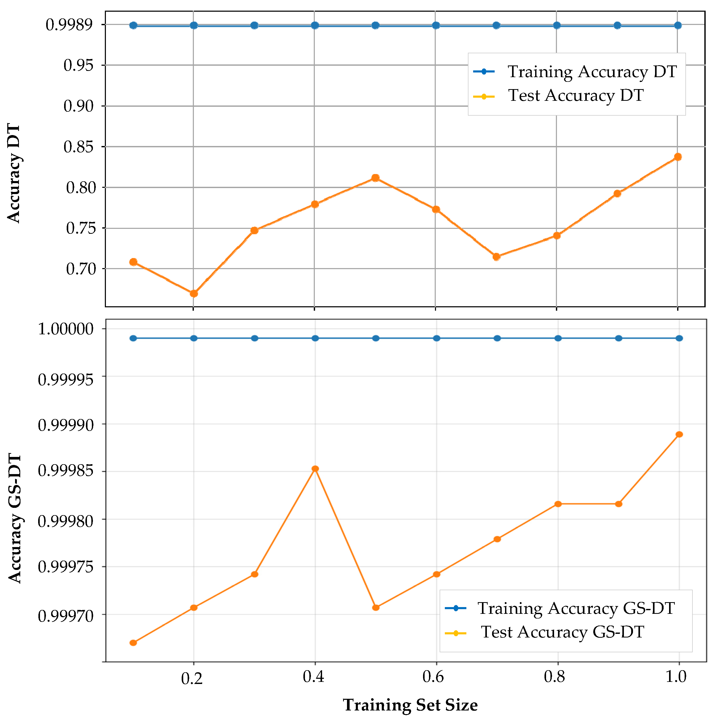
Figure 5 further illustrates this difference through the learning curves of the two models. In the case of the baseline DT, the training accuracy remained equal to 99.998% across all training set sizes, while the test accuracy stayed considerably lower. The persistent gap between the two curves clearly indicates overfitting. By contrast, the optimized GS-DT showed a much smaller discrepancy between training and test performance, which confirms that hyperparameter tuning improved the generalization ability of the model.

Figure 5. Learning curves of the baseline DT and the GS-DT.

The baseline DT exhibits a pronounced gap between training and test accuracy, indicating overfitting, whereas the optimized GS-DT shows a substantially reduced gap and improved generalization. Overall, these results demonstrate that the baseline DT was not sufficiently reliable to serve directly as the model-based labeling component of the ALP. The application of GS significantly reduced overfitting and produced a more robust classifier, making the GS-DT more suitable for the subsequent validation and iterative refinement stages of the proposed methodology.

4.2. Analysis of the GS-DT Results

After hyperparameter optimization, illustrated in Table 3, the GS-DT model was adopted as the primary classifier within the proposed ALP.

Table 3. Hyperparameters selected by Grid Search.

Parameter	Description	Values Tested	Selected Value
max_depth	Maximum depth of the Decision Tree	[None, 10, 20, 30]	10
min_samples_split	Minimum number of samples required to split an internal node	[2, 5, 10]	2
min_samples_leaf	Minimum number of samples required at a leaf node	[1, 2, 4]	1
criterion	Function to measure the quality of a split	[‘gini’, ‘entropy’]	gini

At iteration t, the set of misclassified samples was defined as

$${\mathcal{M}}^{\left(\mathrm{t}\right)}=\left\{\mathrm{i}\hspace{0.25em}\mid \hspace{0.25em}{\widehat{\mathrm{y}}}_{\mathrm{i}}^{\left(\mathrm{t}\right)}≠{\mathrm{y}}_{\mathrm{i}}^{\left(\mathrm{t}\right)}\right\},$$

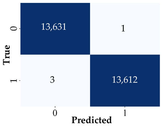
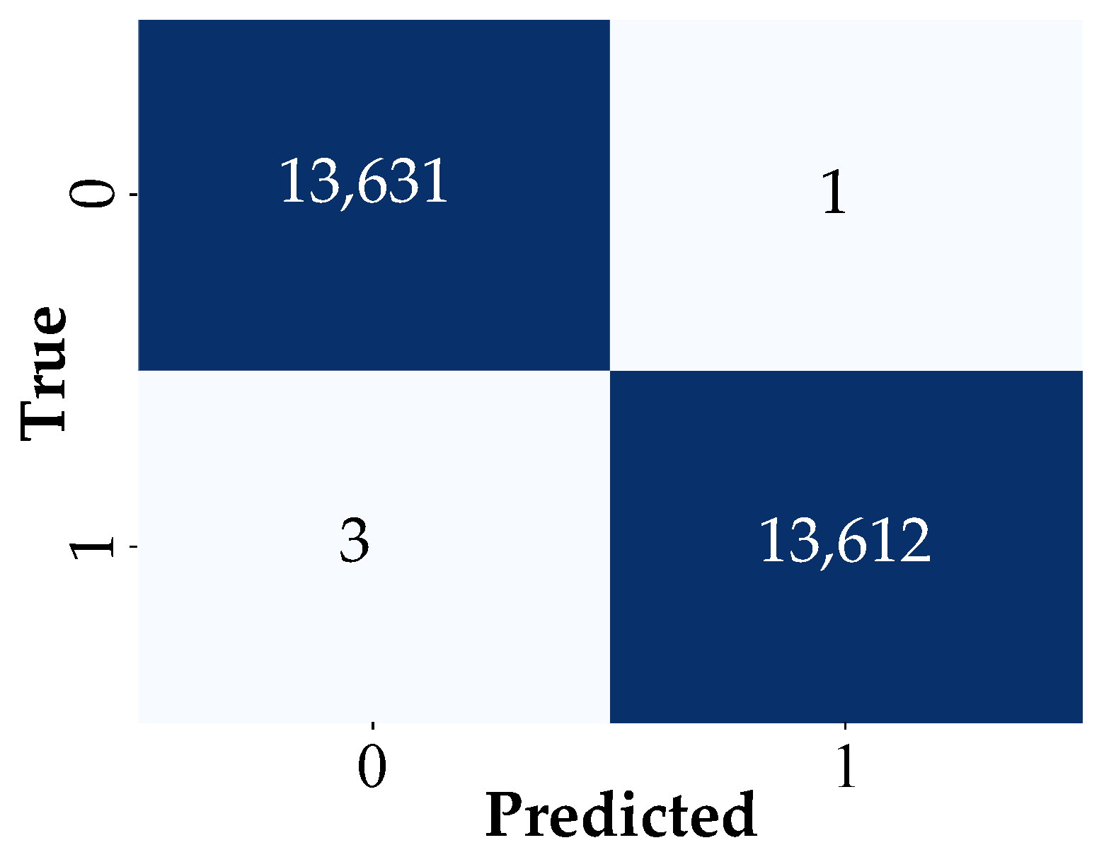
The confusion matrix of the GS-DT model (Figure 6) showed that ${\mathcal{M}}^{\left(\mathrm{t}\right)}=4$, consisting of three false positives (FPs) and one false negative (FN). This small cardinality made manual verification feasible. Each sample was reviewed using its SCADA feature values and its timestamp relative to the gearbox-changeout interval.

Figure 6. Confusion matrix of the GS-DT model before relabeling.

The analysis revealed that not all misclassified samples were of the same nature.

$${\mathcal{M}}^{\left(\mathrm{t}\right)}=\complement$$

The corresponding misclassified samples are listed in Table 4.

Table 4. Disputed samples identified by the misclassification-guided ALP refinement loop.

Type	Reference	Wind Speed (m/s)	Wind DirAbs (deg)	Power (kW)	Max Power (kW)	Min Power (kW)	StdDev Power (kW)	GearOilTemp (°C)	GearBearTemp (°C)
FP	561216	6.0	248.1	110.2	435.5	22.3	72.2	51	59
FP	561231	7.2	240.7	194.3	280.3	145.7	27.0	57	65
FP	558677	5.3	145.0	−0.6	−0.6	−4.5	0.3	18	18
FN	625402	0.0	−1152.6	3072.6	−3276.8	3276.7	0.0	0	0

The first two false-positive samples (561216 and 561231), recorded on 5 September 2018, are characterized by positive power output, non-zero variability in power, and gearbox temperatures that are consistent with turbine operation under load. Since these samples also occur outside the gearbox-changeout interval, their feature patterns are more compatible with normal turbine behavior than with a confirmed fault-related state. These two samples can therefore be interpreted as typical mistakes produced by the classifier rather than obvious labeling inconsistencies.

The third false-positive sample (sample 558677), recorded on 22 April 2019, presents a different pattern. This observation exhibits near-zero or slightly negative power output, almost no variation in power, and low gearbox temperatures. In addition, its timestamp falls within the gearbox-changeout interval that was used as the fault-related reference period. Consequently, this sample is more reasonably associated with a non-operational or fault-related condition than with normal turbine operation. Unlike the first two false positives, this case represents a credible candidate for relabeling.

The false-negative sample (625402) identified by the GS-DT model also requires careful interpretation. Its recorded values are highly unusual, including WindDirAbs = −1152.6, Power = 3072.6, MaxPower = −3276.8, MinPower = 3276.7, and zero values for both gearbox temperatures. Such values are physically implausible under normal SCADA operation and suggest the presence of a corrupted record, sensor anomaly, or data-quality issue rather than a meaningful operating state. For this reason, this sample should not be interpreted as a simple classification error alone; instead, it must be treated as a suspicious record requiring targeted verification before any relabeling decision is made.

Thus, the verification process partitioned ${\mathcal{M}}^{\left(\mathrm{t}\right)}$ into three distinct subsets:

$${\mathcal{M}}^{\left(\mathrm{t}\right)}={\mathcal{R}}^{\left(\mathrm{t}\right)}\cup {\complement }^{\left(\mathrm{t}\right)}\cup {\mathsf{A}}^{\left(t\right)}$$

where

• ${\mathcal{R}}^{\left(\mathrm{t}\right)}=\left\{558677\right\}$: justified relabeling candidates;
• ${\complement }^{\left(\mathrm{t}\right)}=\left\{561216, 561231\right\}$: confirmed correct labels despite model error;
• ${\mathsf{A}}^{\left(t\right)}=\left\{624502\right\}$: data-quality anomalies requiring separate handling.

4.3. Relabeling the Dataset and Iterative Refinement

The GS-DT model produced only four disputed samples, which made manual verification feasible. Each sample was reviewed using its SCADA feature values and its timestamp relative to the gearbox-changeout interval.

Following the selective relabeling strategy of the ALP, relabeling was performed only for samples whose inconsistency was considered justified after verification.

The subset selected for relabeling was determined using the label update rule described in Section 2.3.3.

For sample 558677,

$${\mathrm{y}}_{\mathrm{i}}^{\left(\mathrm{t}\right)}=0 ⟹{\mathrm{y}}_{\mathrm{i}}^{\left(\mathrm{t}+1\right)}=1$$

For samples 561216 and 561231, the original labels were retained:

$${\mathrm{y}}_{\mathrm{i}}^{\left(\mathrm{t}\right)}={\mathrm{y}}_{\mathrm{i}}^{\left(\mathrm{t}+1\right)}=0$$

For sample 625402, the original label was also retained at this stage, but the sample was selected for manual review rather than being treated as a confirmed correct label:

$${\mathrm{y}}_{\mathrm{i}}^{\left(\mathrm{t}\right)}={\mathrm{y}}_{\mathrm{i}}^{\left(\mathrm{t}+1\right)}=1$$

With $y=0$ denoting Normal and $y=1$ denoting Fault, the label updates after verification are summarized in Table 5.

Table 5. Verification decisions and selective label updates for disputed samples.

Type	Reference	${\mathbf{y}}_{\mathbf{i}}^{\mathbf{\left(}\mathit{t}\mathbf{\right)}}$	StdDev Power (KW)	${\mathbf{y}}_{\mathbf{i}}^{\left(\mathbf{t}+1\right)}$
FP	561216	0	Retained as Normal	0
FP	561231	0	Retained as Normal	0
FP	558677	0	Retained as Fault	1
FN	625402	1	Kept under manual review/not automatically changed	1

The relabeled dataset for the next iteration was constructed as

$${\mathcal{D}}_{\mathrm{r}\mathrm{e}\mathrm{l}\mathrm{a}\mathrm{b}\mathrm{e}\mathrm{l}\mathrm{e}\mathrm{d}}^{\left(\mathrm{t}+1\right)}={\left\{({\mathrm{z}}_1,{\mathrm{y}}_1^{\left(\mathrm{t}+1\right)}),({\mathrm{z}}_2,{\mathrm{y}}_2^{\left(\mathrm{t}+1\right)}),\dots ,({\mathrm{z}}_{\mathrm{i}},{\mathrm{y}}_{\mathrm{i}}^{\left(\mathrm{t}+1\right)}),\dots ,({\mathrm{z}}_{{\mathrm{N}}_B},{\mathrm{y}}_{{\mathrm{N}}_B}^{\left(\mathrm{t}+1\right)})\right\}}^T,$$

The convergence criterion for the ALP requires two conditions:

• Label stability condition:

  $$\left|{\mathcal{R}}^{\left(t\right)}\right|=0$$
• Performance stability condition:

  $$\mid {\mathrm{F}}_1^{\left(\mathrm{t}+1\right)}-{\mathrm{F}}_1^{\left(\mathrm{t}\right)}\mid <\mathsf{\epsilon },$$

Since $\mid {\mathcal{R}}^{\left(\mathrm{t}\right)}\mid =1\ne 0$, the label stability condition was not satisfied at this iteration. Therefore, the refinement loop continued. The sample 558677 was successfully relabeled from Normal to Fault, while the other three misclassified samples were either confirmed as correct or flagged for special handling. The iterative procedure would proceed to iteration $\mathrm{t}+1$ with the updated dataset, after which the same cycle of validation, misclassification analysis, and selective relabeling would be repeated until convergence. The refined dataset was evaluated again to determine whether the convergence criteria had been satisfied using RF and XGBoost classifiers alongside the GS-DT.

4.4. Comparative Verification Using Random Forest and XGBoost

After the first relabeling step based on the GS-DT analysis, the updated dataset ${\mathcal{D}}_{\mathrm{r}\mathrm{e}\mathrm{l}\mathrm{a}\mathrm{b}\mathrm{e}\mathrm{l}\mathrm{e}\mathrm{d}}^{\left(\mathrm{t}+1\right)}$ was further evaluated using (RF) and XGBoost to verify the consistency of the refined labels. The purpose of this stage was not to replace the GS-DT as the main classifier within the ALP, but to confirm whether the remaining disputed samples were still identified by other strong classifiers. In this way, RF and XGB were used as verification models in the iterative refinement process.

At this stage, for each verification model $\mathrm{m}\in \{\mathrm{RF},\mathrm{XGB}\}$, the set of misclassified samples was defined as

$${\mathcal{M}}_m^{(t+1)}=\left\{\mathrm{i}\hspace{0.25em}\mid \hspace{0.25em}{\widehat{\mathrm{y}}}_{\mathrm{i},\mathrm{m}}^{\left(\mathrm{t}+1\right)}≠{\mathrm{y}}_{\mathrm{i}}^{\left(\mathrm{t}+1\right)}\right\},$$

where ${\widehat{\mathrm{y}}}_{\mathrm{i},\mathrm{m}}^{\left(\mathrm{t}+1\right)}$ denotes the label predicted by verification model $m$ on the refined dataset.

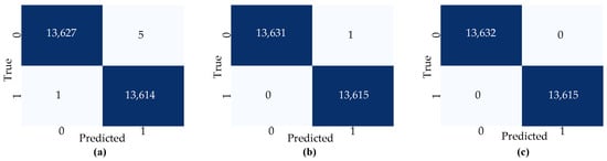
The confusion matrices obtained after the first relabeling presented in Figure 7 showed

Figure 7. Confusion matrices of the evaluated models after the first relabeling step: (a) Random Forest, (b) XGBoost, and (c) GS-DT.

• GS-DT: $\left|{\mathcal{M}}_{GS-DT}^{(t+1)}\right|=$ 0 (zero false positives, zero false negatives);
• Random Forest: $\left|{\mathcal{M}}_{RF}^{(t+1)}\right|=$ 6 (five false positives, one false negative);
• XGBoost: $\left|{\mathcal{M}}_{XGB}^{(t+1)}\right|=$ 1 (one false positive, zero false negatives).

A more detailed examination of these samples showed that the false-negative cases identified by RF and XGBoost (samples 621237, 581705, 621109, 581697, and 621240) occurred during the gearbox-changeout interval. Since this period had already been established as a confirmed fault-related operational interval, all samples within it should be assigned to the Fault class $y=1$. Accordingly, these samples

$${\mathrm{y}}_{\mathrm{i}}^{\left(\mathrm{t}+1\right)}=0 \left(\mathrm{Normal}\right), \mathrm{but} \mathrm{should} \mathrm{be} 1 \left(\mathrm{Fault}\right)$$

Therefore, these disputed observations were interpreted as remaining labeling inconsistencies rather than ordinary model errors alone.

The remaining disputed samples identified by RF and XGBoost are summarized in Table 6.

Table 6. Misclassified samples identified by Random Forest and XGBoost after the first relabeling step.

Model	Type	Reference	Wind Speed	Wind DirAbs	Power	Max Power	Min Power	StdDev Power	GearOilTemp	GearBearTemp
RF	FN	621237	6.6	241.3	136.9	315.8	−7.7	77.3	27	40
RF	FN	581705	4.5	233.4	38.2	90.4	−7.8	19.7	51	59
RF	FN	621109	8.0	146.0	289.5	590.8	125.7	87.9	36	62
RF	FN	581697	5.3	258.2	72.2	288.7	15.5	62.8	52	60
RF	FN	621240	1.1	146.9	298.0	35.9	58.8	32.0	58	-
RF	FP	625402	0.0	−1152.6	3072.6	−3276.8	3276.7	0.0	0	0
XGB	FN	581697	5.5	258.2	72.2	288.7	15.5	62.8	52	60

The only false-positive sample (reference 625402) displayed physically implausible feature values, including extreme and contradictory power-related values and zero gearbox temperatures. This record was therefore treated as a suspicious data-quality anomaly ${\mathrm{i}\mathsf{ϵ}\mathsf{A}}^{(t+1)}$, requiring special consideration, rather than as a straightforward operating-state sample.

$${\mathcal{R}}^{\left(\mathrm{t}+1\right)}=\left\{\mathrm{621237,581705,621109,581697,621240}\right\}, \left|{\mathcal{R}}^{\left(\mathrm{t}+1\right)}\right|=5\ne 0$$

Sample 625402 was not included in ${\mathcal{R}}^{\left(\mathrm{t}+1\right)}$ due to data-quality issues.

The label update rule for iteration $\mathrm{t}+1$ was applied as

$${\mathrm{y}}_{\mathrm{i}}^{\left(\mathrm{t}+2\right)}=\left\{\begin{array}{cc}{\widehat{\mathrm{y}}}_{\mathrm{i}}^{\left(\mathrm{t}+1\right)},& \mathrm{i}\in {\mathcal{R}}^{\left(\mathrm{t}+1\right)}\\ {\mathrm{y}}_{\mathrm{i}}^{\left(\mathrm{t}+1\right)},& \mathrm{i}\notin {\mathcal{R}}^{\left(\mathrm{t}+1\right)}\end{array}\right.$$

Since ${\widehat{\mathrm{y}}}_{\mathrm{i}}^{\left(\mathrm{t}+1\right)}=1$ (Fault) for these five samples (they were predicted as Fault by the verification models), and their current labels were ${\mathrm{y}}_{\mathrm{i}}^{\left(\mathrm{t}+1\right)}=0$ (Normal), the update yielded

$${\mathrm{y}}_{\mathrm{i}}^{\left(\mathrm{t}+2\right)}=2\mathrm{for} \mathrm{all} \mathrm{i}\notin {\mathcal{R}}^{\left(\mathrm{t}+1\right)}$$

Overall, the results obtained from RF and XGBoost provide additional support for the ALP refinement logic. After the first relabeling step, the number of disputed samples was reduced to a very small subset, and the remaining disagreements were concentrated in observations that either belonged to the gearbox-changeout period or exhibited abnormal data patterns. This confirms that the iterative relabeling process improved dataset consistency and that the refined labels were largely supported by multiple classifiers.

4.5. Verification and Convergence of the ALP

After the second relabeling step (iteration), the ALP was re-evaluated using Random Forest, XGBoost, and the GS-DT to verify whether any additional justified relabeling was still required.

At this stage, for each verification model $\mathrm{m}\in \{\mathrm{RF},\mathrm{XGB}\}$, the set of misclassified samples was defined as

$${\mathcal{M}}_m^{(t+2)}=\left\{\mathrm{i}\hspace{0.25em}\mid \hspace{0.25em}{\widehat{\mathrm{y}}}_{\mathrm{i},\mathrm{m}}^{\left(\mathrm{t}+2\right)}≠{\mathrm{y}}_{\mathrm{i}}^{\left(\mathrm{t}+2\right)}\right\},$$

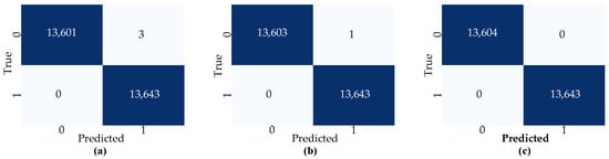
The resulting confusion matrices are presented in Figure 8.

Figure 8. Confusion matrices of the evaluated models after the final relabeling step: (a) Random Forest, (b) XGBoost, and (c) GS-DT.

• GS-DT: $\left|{\mathcal{M}}_{GS-DT}^{(t+2)}\right|=$ 0 (perfect classification);
• Random Forest: $\left|{\mathcal{M}}_{RF}^{(t+2)}\right|=$ 3 (five false positives, one false negative);
• XGBoost: $\left|{\mathcal{M}}_{XGB}^{(t+2)}\right|=$ 1 (one false positive, zero false negatives).

A detailed review of these remaining disputed samples indicated that they had already been examined in the previous refinement steps and did not justify additional relabeling. Their feature values did not provide sufficient evidence to overturn the current assigned labels with confidence. Therefore,

$$\left|{\mathcal{R}}^{\left(\mathrm{t}+2\right)}\right|=0$$

From the perspective of the ALP, this stage marks the convergence of the iterative process. The stopping criteria defined in the general ALP formulation were satisfied:

• Label stability condition:

  $$\left|{\mathcal{R}}^{\left(t+2\right)}\right|=0$$
• Performance stability condition:

  $$\mid {\mathrm{F}}_1^{\left(\mathrm{t}+2\right)}-{\mathrm{F}}_1^{\left(1\right)}\mid <\mathsf{\epsilon },$$

where $\mathsf{\epsilon }$ is a predefined tolerance. Since no additional justified relabeling actions remained and the model performance no longer showed meaningful improvement, both conditions were met.

The refined dataset obtained at this stage was therefore accepted as the final labeled dataset produced by the proposed ALP:

$${{\mathcal{D}}_{\mathrm{r}\mathrm{e}\mathrm{l}\mathrm{a}\mathrm{b}\mathrm{e}\mathrm{l}\mathrm{e}\mathrm{d}}^{*}=\mathcal{D}}_{\mathrm{r}\mathrm{e}\mathrm{l}\mathrm{a}\mathrm{b}\mathrm{e}\mathrm{l}\mathrm{e}\mathrm{d}}^{\left(\mathrm{t}+2\right)}={\left\{({\mathrm{z}}_1,{\mathrm{y}}_1^{\left(\mathrm{t}+2\right)}),({\mathrm{z}}_2,{\mathrm{y}}_2^{\left(\mathrm{t}+2\right)}),\dots ,({\mathrm{z}}_{\mathrm{i}},{\mathrm{y}}_{\mathrm{i}}^{\left(\mathrm{t}+2\right)}),\dots ,({\mathrm{z}}_{{\mathrm{N}}_B},{\mathrm{y}}_{{\mathrm{N}}_B}^{\left(\mathrm{t}+2\right)})\right\}}^T,$$

The remaining disputed samples are summarized in Table 7.

Table 7. Remaining disputed samples after the final relabeling step.

Model	Type	Reference	Wind Speed	WindDirAbs	Power	Max Power	Min Power	StdDev Power	GearOilTemp	GearBearTemp
Random Forest	FP	621237	6.6	241.3	136.9	315.8	−7.7	77.3	27	40
Random Forest	FP	621109	8.0	146.0	289.5	590.8	125.7	87.9	36	62
Random Forest	FP	621240	1.1	146.9	298.0	35.9	58.8	32.0	58	—
XGBoost	FP	581697	5.5	258.2	72.2	288.7	15.5	62.8	52	60

4.6. Additional Validation of the ALP

Two complementary validation experiments were conducted to evaluate the results of the proposed ALP. First, a Gradient Boosting Classifier was applied to the final relabeled dataset to determine whether the refined labels remained consistently learnable using a model that was not involved in the iterative relabeling procedure. Second, the frozen GS-DT was applied to a chronologically unseen SCADA period to evaluate whether the proposed approach could generate initial prelabels without using the operational-state labels of that period during model development. The first experiment evaluates the internal consistency of the final relabeled dataset, whereas the second evaluates the practical deployment of the ALP on unseen data.

4.6.1. Evaluation of the Final Relabeled Dataset Using Gradient Boosting

To provide an additional evaluation of the final relabeled dataset, a Gradient Boosting Classifier (GBC) was applied after completion of the ALP refinement process. The GBC was not involved in the iterative relabeling procedure. Instead, it was used as an independent evaluation model to determine whether the final refined labels remained consistently learnable using another ensemble-learning approach.

The GBC was evaluated under the same experimental conditions used for the other classifiers. The same final relabeled and balanced SCADA dataset, selected input features, class definitions, 60%/20%/20% training–validation–test partition, and random state were retained. In all experiments, (y = 0) represents normal operation and (y = 1) represents the fault-related state. Performance was assessed using accuracy, precision, recall, F1-score, and confusion-matrix analysis.

On the test set, the GBC achieved an accuracy of 99.9245%. For the fault-related class, the precision, recall, and F1-score were 99.9371%, 99.9119%, and 99.9245%, respectively. The test set contained 15,896 observations, with 7948 samples from each class, as reported in Table 8.

Table 8. Test performance of the GBC on the final relabeled dataset.

Model	Accuracy	Precision	Recall	F1-Score
GBC	99.9245%	99.9371%	99.9119%	99.9245%

The confusion matrix showed that 7943 normal observations and 7941 fault-related observations were correctly classified. Five normal samples were classified as fault-related, corresponding to false-positive predictions, while seven fault-related samples were classified as normal, corresponding to false-negative predictions. In total, the GBC produced 12 misclassified observations, as shown in Table 9.

Table 9. Confusion matrix of the Gradient Boosting Classifier on the final relabeled test set.

True Class	Predicted Normal	Predicted Fault-Related
Normal	7943	5
Fault-related	7	7941

These results indicate that the final relabeled dataset can be learned with high consistency by an additional ensemble classifier. The limited number of disagreements provides further support for the stability of the labels obtained through the ALP. However, model disagreements were not treated as labeling errors unless supported by the corresponding timestamps, SCADA measurements, temporal behavior, physical plausibility, and relationship to the documented gearbox-changeout interval.

Although the GBC achieved high predictive performance, the optimized Decision Tree was retained as the principal classifier within the ALP refinement loop because its explicit decision rules facilitate the interpretation of disputed observations. The GBC was therefore used as an independent model for evaluating the consistency of the final relabeled dataset.

The GBC evaluates the consistency of the final labels using a conventional labeled test set. However, it does not directly assess whether the ALP can initiate labeling when the operational state of a new dataset is unknown. This aspect is investigated separately in the following chronological validation.

4.6.2. Validation on a Chronologically Unseen SCADA Period

To assess whether the ALP can initiate the labeling of previously unseen data without prior knowledge of the operational state, the ALP was further evaluated on 10,097 ten-minute Vestas SCADA observations recorded between 1 January and 12 March 2020. The original 2017–2019 case study was used for methodological development and demonstrated how the ALP could refine provisional labels when an initial documented reference interval was available. By contrast, the new 2020 validation set was independent of the original case study and was used to evaluate the automated prelabeling of unseen data without prior state information.

The 2020 period was not used in any form of label derivation, feature selection, class balancing, hyperparameter optimization, validation, or threshold selection. The previously optimized GS-DT was frozen with the Gini criterion, a maximum depth of 10, a minimum split size of 2, and a minimum leaf size of 1.

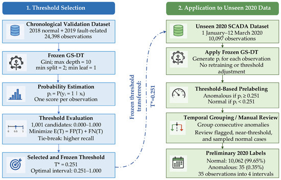
For each observation ${\mathrm{x}}_{\mathrm{i}}$, the model generated a changeout-related probability ${\mathrm{p}}_{\mathrm{i}}=\mathrm{P}\left({\mathrm{y}}_{\mathrm{i}}=1\mid {\mathrm{x}}_{\mathrm{i}}\right)$. The decision threshold was selected before using a separate chronological validation set of 24,398 observations from January–March 2018 and January–March 2019. A total of 1001 candidate thresholds were evaluated over $\mathrm{T}=\{\mathrm{0,0.001},\dots ,1.000\}$. For each threshold, the validation error was calculated as $\mathrm{E}\left(\mathrm{T}\right)=\mathrm{F}\mathrm{P}\left(\mathrm{T}\right)+\mathrm{F}\mathrm{N}\left(\mathrm{T}\right)$.

The threshold minimizing $\mathrm{E}\left(\mathrm{T}\right)$ was retained, with higher fault-related recall used to resolve ties. This procedure gives ${\mathrm{T}}^{*}=0.251$. At this threshold, the validation set produced 11,914 true negatives, 102 false positives, 1080 false negatives, and 11,302 true positives, corresponding to 95.1553% accuracy, 99.1056% precision, 91.2777% recall, and a 95.0307% F1-score, as presented in Table 10.

Table 10. Performance of the GS-DT on the chronological validation subset at (T* = 0.251).

Observations	TN	FN	PN	PF	Accuracy	Balanced Accuracy	Precision	Recall	F1-Score
24,398	11,914	102	1080	11,302	95.1553%	95.2144%	99.1056%	91.2777%	95.0307%

The frozen threshold was then applied to the unseen 2020 observations according to

$${\widehat{\mathrm{y}}}_{\mathrm{i}}=\left\{\begin{array}{cc}1,& {\mathrm{p}}_{\mathrm{i}}\ge 0.251,\\ 0,& {\mathrm{p}}_{\mathrm{i}}<0.251.\end{array}\right.$$

Only preliminary labels were generated at this stage. As illustrated in Figure 9, the workflow comprised probability estimation, threshold-based prelabeling, grouping of consecutive anomalous predictions, and manual verification using temporal context and physically meaningful operating variables. The model assigned 10,062 observations to the preliminary normal class and 35 to the preliminary anomalous class.

Figure 9. Chronological validation workflow for unseen SCADA data.

Thus, 35 of the 10,097 observations, corresponding to 0.35% of the unseen dataset, were prioritized for immediate review. These observations formed four intervals. Manual verification showed that 33 observations exhibited stopped or standby-like behavior, while two remained uncertain. The audit also included four near-threshold observations and 55 high-confidence normal predictions. Among the latter, 44 were consistent with normal power production, whereas 11 exhibited stopped, transitional, or uncertain behavior requiring further examination.

The two evaluations therefore support different conclusions. The original case study shows that the ALP can refine provisional labels when an initial documented reference interval is available. The independent chronological validation shows that the same frozen framework can initiate probability-based prelabeling on a later unseen period without prior knowledge of its operational states. The 2020 observations were not used to derive the labels; instead, the generated prelabels were subsequently checked using temporal and physical operating context.

These findings support the probability-based prelabeling principle used in the original case study. The frozen GS-DT and threshold isolated a small, operationally distinct subset from unseen data without prior knowledge of its states, reducing the immediate review workload from 10,097 to 35 observations. However, the probability represents similarity to the learned changeout-related operating pattern rather than the probability of a confirmed gearbox failure, and the generated labels remain preliminary owing to the absence of independent maintenance and alarm records.

4.7. Discussion

The obtained results confirm that the proposed ALP is effective for identifying and correcting potentially inconsistent labels in wind turbine SCADA datasets. The initial DT classifier achieved very high performance, with only four misclassified samples out of 27,247 test observations, indicating that the selected SCADA features provide strong separation between Normal and Fault operating states.

Among the considered variables, rotor speed, generator speed, and gearbox temperatures were the most influential indicators because they are directly related to turbine mechanical behavior and gearbox condition. The analysis of the four disputed samples showed that three false positives were associated with transition conditions, while one false negative, sample 625402, contained physically implausible values, suggesting a data-quality anomaly rather than a typical operating-state sample. After selective relabeling and model retraining, the number of disputed samples remained very small, demonstrating fast convergence of the ALP. Comparative verification using RF and XGBoost further supported the relabeling decisions, showing that the refined labels remained consistent across different classification models.

Future work will investigate an unsupervised initialization of the ALP using multivariable SCADA anomaly thresholds when documented maintenance or failure information is unavailable.

5. Conclusions

This manuscript presented an Automated Labeling Procedure (ALP) for wind turbine SCADA data, aimed at constructing a reliable labeled dataset from initially unlabeled operational records. Unlike conventional supervised-learning workflows, in which labels are assumed to be fixed, the proposed ALP treats these labels as provisional and progressively refines them through validation, misclassification analysis, selective relabeling, and retraining.

The main contribution of this study is the misclassification-guided refinement loop, which converts model disagreements into a controlled label verification process. Instead of automatically accepting model predictions, the ALP analyzes disputed samples, selectively updates only justified labels, flags abnormal records requiring manual review, and retrains the model until the refined label set becomes stable. The proposed procedure was applied to a real wind turbine SCADA dataset containing a gearbox-changeout interval used as the initial fault-related reference period. In the model-based validation stage, a Decision Tree optimized by Grid Search (GS-DT) was employed as the primary classifier because of its interpretability and suitability for identifying suspicious observations through explicit decision rules. The baseline Decision Tree exhibited overfitting, whereas the optimized GS-DT showed a substantial improvement in generalization, reaching 99.985% accuracy, 99.993% precision, 99.978% recall, and 99.985% F1-score. These results confirmed the suitability of the GS-DT as the main validation model within the ALP.

The main advantage of the proposed algorithm lies in its iterative nature and, above all, in focusing only on a small subset of disputed samples. After successive relabeling steps, the number of disputed samples decreased, and the results stabilized across the GS-DT, Random Forest, and XGBoost, indicating convergence of the refinement loop. In addition, chronological validation on a later SCADA period demonstrated that the frozen ALP could generate preliminary labels for previously unseen data without using the operational-state labels of that period during model development. This provides direct evidence of the method’s practical labeling capability beyond the original case-study interval. The present study used documented operational information to initialize the ALP; when such information is unavailable, future implementations may employ feature-based statistical, physical, or unsupervised thresholds to generate candidate anomaly-based prelabels requiring expert or operational verification. Overall, the results demonstrate that the ALP can refine provisional SCADA labels and reduce the manual effort required for label verification while improving dataset consistency.

References

- Du, B.; Narusue, Y.; Furusawa, Y.; Nishihara, N.; Indo, K.; Morikawa, H.; Iida, M. Clustering Wind Turbines for SCADA Data-Based Fault Detection. IEEE Trans. Sustain. Energy 2023, 14, 442–452. [Google Scholar] [CrossRef] [Scilit]
- Osman, A.I.; Chen, L.; Yang, M.; Msigwa, G.; Farghali, M.; Fawzy, S.; Rooney, D.W.; Yap, P.-S. Cost, Environmental Impact, and Resilience of Renewable Energy under a Changing Climate: A Review. Environ. Chem. Lett. 2023, 21, 741–764. [Google Scholar] [CrossRef] [Scilit]
- Dinh, V.N.; McKeogh, E. Offshore Wind Energy: Technology Opportunities and Challenges. In Proceedings of the 1st Vietnam Symposium on Advances in Offshore Engineering; Randolph, M.F., Doan, D.H., Tang, A.M., Bui, M., Dinh, V.N., Eds.; Springer: Singapore, 2019; pp. 3–22. [Google Scholar]
- Snyder, B.; Kaiser, M.J. Ecological and Economic Cost-Benefit Analysis of Offshore Wind Energy. Renew. Energy 2009, 34, 1567–1578. [Google Scholar] [CrossRef] [Scilit]
- Chen, X.; Yan, R.; Liu, Y. Wind Turbine Condition Monitoring and Fault Diagnosis in China. IEEE Instrum. Meas. Mag. 2016, 19, 22–28. [Google Scholar] [CrossRef] [Scilit]
- Helbing, G.; Ritter, M. Deep Learning for Fault Detection in Wind Turbines. Renew. Sustain. Energy Rev. 2018, 98, 189–198. [Google Scholar] [CrossRef] [Scilit]
- Jin, X.; Xu, Z.; Qiao, W. Condition Monitoring of Wind Turbine Generators Using SCADA Data Analysis. IEEE Trans. Sustain. Energy 2021, 12, 202–210. [Google Scholar] [CrossRef] [Scilit]
- Kusiak, A.; Zhang, Z.; Verma, A. Prediction, Operations, and Condition Monitoring in Wind Energy. Energy 2013, 60, 1–12. [Google Scholar] [CrossRef] [Scilit]
- Yang, W.; Tavner, P.J.; Crabtree, C.J.; Feng, Y.; Qiu, Y. Wind Turbine Condition Monitoring: Technical and Commercial Challenges. Wind Energy 2014, 17, 673–693. [Google Scholar] [CrossRef] [Scilit]
- Zaher, A.; McArthur, S.D.J.; Infield, D.G.; Patel, Y. Online Wind Turbine Fault Detection through Automated SCADA Data Analysis. Wind Energy 2009, 12, 574–593. [Google Scholar] [CrossRef] [Scilit]
- Santolamazza, A.; Dadi, D.; Introna, V. A Data-Mining Approach for Wind Turbine Fault Detection Based on SCADA Data Analysis Using Artificial Neural Networks. Energies 2021, 14, 1845. [Google Scholar] [CrossRef] [Scilit]
- Uluyol, O.; Parthasarathy, G.; Foslien, W.; Kim, K. Power Curve Analytic for Wind Turbine Performance Monitoring and Prognostics. Annu. Conf. PHM Soc. 2011, 3. [Google Scholar] [CrossRef] [Scilit]
- Dempsey, P.J.; Sheng, S. Investigation of Data Fusion Applied to Health Monitoring of Wind Turbine Drivetrain Components. Wind Energy 2013, 16, 479–489. [Google Scholar] [CrossRef] [Scilit]
- Schlechtingen, M.; Santos, I.F.; Achiche, S. Using Data-Mining Approaches for Wind Turbine Power Curve Monitoring: A Comparative Study. IEEE Trans. Sustain. Energy 2013, 4, 671–679. [Google Scholar] [CrossRef] [Scilit]
- Chatterjee, J.; Dethlefs, N. Scientometric Review of Artificial Intelligence for Operations & Maintenance of Wind Turbines: The Past, Present and Future. Renew. Sustain. Energy Rev. 2021, 144, 111051. [Google Scholar] [CrossRef] [Scilit]
- Kim, B.; Alawami, M.A.; Kim, E.; Oh, S.; Park, J.; Kim, H. A Comparative Study of Time Series Anomaly Detection Models for Industrial Control Systems. Sensors 2023, 23, 1310. [Google Scholar] [CrossRef] [Scilit] [PubMed]
- Okaro, I.A.; Jayasinghe, S.; Sutcliffe, C.; Black, K.; Paoletti, P.; Green, P.L. Automatic Fault Detection for Laser Powder-Bed Fusion Using Semi-Supervised Machine Learning. Addit. Manuf. 2019, 27, 42–53. [Google Scholar] [CrossRef] [Scilit]
- Gilanifar, M.; Wang, H.; Cordova, J.; Ozguven, E.E.; Strasser, T.I.; Arghandeh, R. Fault Classification in Power Distribution Systems Based on Limited Labeled Data Using Multi-Task Latent Structure Learning. Sustain. Cities Soc. 2021, 73, 103094. [Google Scholar] [CrossRef] [Scilit]
- Tang, M.; Zhao, Q.; Ding, S.X.; Wu, H.; Li, L.; Long, W.; Huang, B. An Improved LightGBM Algorithm for Online Fault Detection of Wind Turbine Gearboxes. Energies 2020, 13, 807. [Google Scholar] [CrossRef] [Scilit]
- Schlechtingen, M.; Santos, I.F.; Achiche, S. Wind Turbine Condition Monitoring Based on SCADA Data Using Normal Behavior Models. Part 1: System Description. Appl. Soft Comput. 2013, 13, 259–270. [Google Scholar] [CrossRef] [Scilit]
- Schlechtingen, M.; Santos, I.F. Wind Turbine Condition Monitoring Based on SCADA Data Using Normal Behavior Models. Part 2: Application Examples. Appl. Soft Comput. 2014, 14, 447–460. [Google Scholar] [CrossRef] [Scilit]
- Tautz-Weinert, J.; Watson, S.J. Using SCADA Data for Wind Turbine Condition Monitoring–a Review. IET Renew. Power Gener. 2017, 11, 382–394. [Google Scholar]
- Yang, W.; Court, R.; Jiang, J. Wind Turbine Condition Monitoring by the Approach of SCADA Data Analysis. Renew. Energy 2013, 53, 365–376. [Google Scholar] [CrossRef] [Scilit]
- Pandit, R.; Astolfi, D.; Hong, J.; Infield, D.; Santos, M. SCADA Data for Wind Turbine Data-Driven Condition/Performance Monitoring: A Review on State-of-Art, Challenges and Future Trends. Wind Eng. 2023, 47, 422–441. [Google Scholar] [CrossRef] [Scilit]
- Chatterjee, S.; Byun, Y.-C. Leveraging Generative Adversarial Networks for Data Augmentation to Improve Fault Detection in Wind Turbines with Imbalanced Data. Results Eng. 2025, 25, 103991. [Google Scholar] [CrossRef] [Scilit]
- Chawla, N.V.; Bowyer, K.W.; Hall, L.O.; Kegelmeyer, W.P. SMOTE: Synthetic Minority Over-Sampling Technique. J. Artif. Intell. Res. 2002, 16, 321–357. [Google Scholar] [CrossRef] [Scilit]
- Han, H.; Wang, W.-Y.; Mao, B.-H. Borderline-SMOTE: A New Over-Sampling Method in Imbalanced Data Sets Learning. In Advances in Intelligent Computing; Huang, D.-S., Zhang, X.-P., Huang, G.-B., Eds.; Lecture Notes in Computer Science; Springer: Berlin/Heidelberg, Germany, 2005; Volume 3644, pp. 878–887. [Google Scholar]
- He, H.; Bai, Y.; Garcia, E.A.; Li, S. ADASYN: Adaptive Synthetic Sampling Approach for Imbalanced Learning. In Proceedings of the 2008 IEEE International Joint Conference on Neural Networks (IEEE World Congress on Computational Intelligence); IEEE: Hong Kong, China, 2008; pp. 1322–1328. [Google Scholar]
- Douzas, G.; Bacao, F.; Last, F. Improving Imbalanced Learning through a Heuristic Oversampling Method Based on K-Means and SMOTE. Inf. Sci. 2018, 465, 1–20. [Google Scholar] [CrossRef] [Scilit]
- Dablain, D.; Krawczyk, B.; Chawla, N.V. DeepSMOTE: Fusing Deep Learning and SMOTE for Imbalanced Data. IEEE Trans. Neural Netw. Learn. Syst. 2023, 34, 6390–6404. [Google Scholar] [CrossRef] [Scilit] [PubMed]
- Ando, S.; Huang, C.Y. Deep Over-Sampling Framework for Classifying Imbalanced Data. In Machine Learning and Knowledge Discovery in Databases; Ceci, M., Hollmén, J., Todorovski, L., Vens, C., Džeroski, S., Eds.; Lecture Notes in Computer Science; Springer International Publishing: Cham, Switzerland, 2017; Volume 10534, pp. 770–785. [Google Scholar]
- Proceedings of the 2023 International Conference on Intelligent Systems for Communication, IoT and Security: (ICISCoIS 2023): 9–11 February, 2023, PSG College of Technology, Coimbatore 641004, Tamil Nadu, India; Umamaheswari, K., Ed.; IEEE: Piscataway, NJ, USA, 2023. [Google Scholar]
- Abdallah, I.; Dertimanis, V.; Mylonas, H.; Tatsis, K.; Chatzi, E.; Dervili, N.; Worden, K.; Maguire, E. Fault Diagnosis of Wind Turbine Structures Using Decision Tree Learning Algorithms with Big Data. In Safety and Reliability—Safe Societies in a Changing World; CRC Press: London, UK, 2018; pp. 3053–3061. [Google Scholar]
- Bahzad; Adnan Abdulazeez, C. Classification Based on Decision Tree Algorithm for Machine Learning. J. Appl. Sci. Technol. Trends 2021, 2, 20–28. [Google Scholar] [CrossRef] [Scilit]
- Navada, A.; Ansari, A.N.; Patil, S.; Sonkamble, B.A. Overview of Use of Decision Tree Algorithms in Machine Learning. In Proceedings of the 2011 IEEE Control and System Graduate Research Colloquium; IEEE: Shah Alam, Malaysia, 2011; pp. 37–42. [Google Scholar]
- Gridin, I. Automated Deep Learning Using Neural Network Intelligence: Develop and Design PyTorch and TensorFlow Models Using Python; Apress: Berkeley, CA, USA, 2022. [Google Scholar]
- Patel, H.H.; Prajapati, P. Study and Analysis of Decision Tree Based Classification Algorithms. Int. J. Comput. Sci. Eng. 2018, 6, 74–78. [Google Scholar] [CrossRef] [Scilit]
- Alibrahim, H.; Ludwig, S.A. Hyperparameter Optimization: Comparing Genetic Algorithm against Grid Search and Bayesian Optimization. In Proceedings of the 2021 IEEE Congress on Evolutionary Computation (CEC); IEEE: Kraków, Poland, 2021; pp. 1551–1559. [Google Scholar]
- Byrne, R. Vestas V52 Wind Turbine, 10-Minute SCADA Data, 2006–2020; Dundalk Institute of Technology: Dundalk, Ireland, 2022. [Google Scholar]
Disclaimer/Publisher’s Note: The statements, opinions and data contained in all publications are solely those of the individual author(s) and contributor(s) and not of MDPI and/or the editor(s). MDPI and/or the editor(s) disclaim responsibility for any injury to people or property resulting from any ideas, methods, instructions or products referred to in the content. |
© 2026 by the authors. Licensee MDPI, Basel, Switzerland. This article is an open access article distributed under the terms and conditions of the Creative Commons Attribution (CC BY) license.