A Modified Analytical Calculation Model for Mutual Inductance Between Arbitrarily Oriented Solenoid Coils

Abstract

Accurate calculation of mutual inductance (MI) between solenoid coils is essential for system design, but complex geometries and spatial arrangements make it challenging. This paper presents a modified analytical method for calculating the MI between two circular-wound air-core solenoid coils arbitrarily oriented in three-dimensional (3D) space. The analytical model used to calculate the MI between two solenoid coils is based on the use of magnetic vector potential (MVP). The helical structure of the solenoid coils is represented by successive coaxial circular filaments arranged along their central axes. Each filament is represented by an equivalent regular polygon with a sufficient number of sides. The proposed approach allows the MI between two solenoid coils to be calculated using a single analytical formula, without imposing restrictions on the relative positions of the coils, while taking lateral and angular misalignments into account. The modified analytical model is validated for accuracy and applicability by comparing its results with experimental measurements and FEM-based simulation results for coil systems with different diameters, turn numbers, and turn pitches. The MI results for various angular and lateral misalignments are in good agreement with experimental measurements and FEM results. The MI calculation model proposed in this work provides a fast and reliable tool for analyzing the electromagnetic behavior of coupled coil systems, designing inductive power transfer systems, and assessing electromagnetic compatibility.

1. Introduction

Mutual inductance is a key parameter in magnetically coupled coils, and its determination is critical for analyzing coil systems, understanding energy transfer, and evaluating system performance. Solenoid coils are widely used in electromagnetic applications such as transformers, inductive sensors [1], electromagnetic actuators [2], wireless power transfer systems [3,4,5,6,7], RFID-based communication systems and RF transmitter circuits [8,9], superconducting high-field magnetic systems [10,11], and biomedical implants [12,13]. Accurate modeling of the magnetic interaction between coils is therefore of great importance in such systems. In addition, magnetic fields in coupled coil systems significantly influence both the energy transfer and electromagnetic interference (EMI). In EMI filters, the magnetic coupling between inductors is a critical factor affecting the performance. As systems become more compact, accurate modeling these interactions and determining the MI between coils is critical, making it an important topic in electromagnetic design [14,15].

Various methods have been proposed for determining the MI between solenoid coils. Maxwell introduced fundamental analytical formulas for coaxial solenoid coils [16], which were later extended in subsequent studies [17,18]. Later works compared elliptic integral-based exact formulas with series expansion methods and proposed calculation tables for coaxial solenoids [19,20]. In [21,22,23,24] analytical solutions based on Bessel functions are proposed for calculating the MI between solenoid coils, while [25,26,27] present elliptic integral-based solutions for air-core solenoids coils. The scope of the analytical and semi-analytical MI calculation methods reported in the literature and the contribution of the present study are more clearly presented in Table 1, where the related studies are comparatively summarized. The comparison is made under the headings of coil model, analytical approach, solution method, misalignment conditions, and validation method.

Table 1. Comparison of the analytical and semi-analytical MI calculation methods for solenoid coils reported in the literature.

Ref.	Coil Model	Analytical Approach	Solution Method	Misalignment Conditions	Validation Method
[21]	Thin cylindrical solenoids	Bessel functions	Integral formulation based on Bessel functions	Coaxial and parallel-axis noncoaxial cases	Numerical examples
[22]	Thin circular and elliptic solenoids; thick circular and elliptic solenoids	Bessel and Struve functions	Integral formulation involving elliptic integrals and Bessel/Struve functions	Coaxial and parallel-axis noncoaxial cases	Comparison between thin and thick coil analytical solutions
[23]	Thick cylindrical coils	Q-vector potential formulation	Three-dimensional integration of analytical terms	Arbitrary relative position and orientation	Comparison with existing analytical solutions
[24]	Coaxial circular coils with rectangular cross-sections, including solenoid and disk coils	Filament-based formulation using Bessel functions	Integral formulation with numerical evaluation	Coaxial configuration	Comparison with existing analytical solutions, FEM and experimental measurements
[25]	Thin-wall solenoids and disk coils	Complete elliptic integrals and Heuman’s Lambda function	Analytical solution for thin-wall solenoids; analytical/numerical solution for disk coils	Coaxial configuration	Comparison with existing analytical solutions
[26]	Inclined solenoids	Filament method, complete elliptic integrals	Semi-analytical formulation based on filament discretization and numerical integration	Relative position and angular orientation	Numerical examples
[27]	Thin-wall solenoids	Complete elliptic integrals	Generalized calculation algorithm with numerical integration	Non-coaxial configuration with parallel axes	Comparison with existing analytical solutions and experimental measurements
This Work	Circular-wound solenoid coils represented by polygonal turns	Stokes Theorem, Magnetic vector potential	Analytical Method	Arbitrary lateral and angular misalignments in 3D space	Comparison with existing analytical solutions, FEM and experimental measurements

MI of solenoid coils depends on their geometry, spatial position, and winding structure. Most calculation methods in the literature are limited to coaxial or geometrically constrained configurations. Although some studies have considered misaligned or inclined coils, a significant portion of the existing formulations relies on integral expressions involving special functions and requires numerical integration for practical calculation. In contrast, this study presents an analytical calculation model for circular-wound solenoid coils in arbitrary relative positions and orientations, without requiring an additional numerical integration step after the analytical MI expression is obtained. Therefore, accurately determining the MI in arbitrary configurations is critical and constitutes the main objective of this work. This work aims to modify the model proposed in [28], originally for calculating the MI between planar coils, for application to solenoid coils. In the modified model, solenoids are represented as 3D structures of circular filaments along the coil axis, enabling analytical consideration of lateral and angular misalignment effects. The results are expected to support the design and performance evaluation of applications such as inductive power transfer systems, coupled coil structures, and electromagnetic compatibility (EMC) analyses.

The remainder of the paper is organized as follows: Section 2 details the proposed analytical model for calculating the MI between solenoid coils and the mathematical approach used. Section 3 evaluates the performance and applicability of the proposed MI calculation model through the convergence analysis of the polygonal representation, benchmark validation, and 3D MI and MVP plots for coil configurations with various angular and lateral displacements. Section 4 provides measurement and FEM results for validating the proposed analytical model, and examines the variation of MI for primary and secondary coils under different angular and lateral misalignments in 3D space. Finally, Section 5 concludes the paper and discusses the results.

2. Modeling Mutual Inductance for Circular-Wound Solenoid Coils

The main purpose of this section is to present an analytical model that enables the calculation of MI between circular-wound solenoid coils by modifying the model previously developed in [28] for the calculation of MI between planar polygonal coils. In the proposed modified analytical model, each turn of the solenoid coils, assumed to be circular-wound, is geometrically represented using an equivalent polygonal-turn approach with a sufficiently high number of sides. This model for calculating the MI between two circularly wound solenoid coils is capable of accurately calculating the MI even when the coils are laterally and/or angularly misaligned in 3D.

In this work, the MVP is obtained from the Biot–Savart law to determine the MI, and the magnetic flux is subsequently calculated by performing the line integral of the MVP.

2.1. Fundamental Equations

When current flows through one of two coils located in close proximity to each other, some of the magnetic field lines generated around it pass through the surface enclosed by the turns of the second coil, creating magnetic coupling expressed by MI. The MI, which is an indicator of magnetic coupling, is expressed as M = $d\varphi /dI$; however, since air-core coils are considered in this work, the relationship between $\varphi$ and I is linear, and therefore the MI is expressed as in (1).

$$M={\displaystyle \frac{\varphi }{I}}$$

(1)

In this expression, $\varphi$ is the linkage flux that cuts the surface enclosed by the turns of one coil due to the current I passing through another coil. Thus, the MI can be found by calculating the magnetic flux. $\varphi$ depends on the current and the ratio of $\varphi$ to I, which determines the MI, is based on the dimensions and the relative position between the coils. Since magnetic flux is calculated using the magnetic flux density ($\overrightarrow{B}$), $\overrightarrow{B}$ must first be calculated based on the Biot–Savart Law.

$$\varphi ={\int }_S\overrightarrow{B}·d\overrightarrow{S}$$

(2)

$$\overrightarrow{B}={\displaystyle \frac{{\mu }_o}{4\pi }}{\oint }_L{\displaystyle \frac{Id\overrightarrow{\ell }\times {\overrightarrow{a}}_R}{R^2}}$$

(3)

where $d\overrightarrow{S}$ is the differential surface, ${\mu }_o$ the permeability of the free space, $d\overrightarrow{\ell }$ the differential length, R the distance between the turns of two coils that share a MI, and ${\overrightarrow{a}}_R$ the unit vector directed from a point on any turn of one coil to another point on any turn of the other coil. In this work, for the simplicity of calculation, it is preferred to calculate the flux using the magnetic vector potential ($\overrightarrow{A}$) instead of taking surface integrals. For this, the relationship between $\overrightarrow{A}$ and $\overrightarrow{B}$ must be utilized.

$$\nabla \times \overrightarrow{A}=\overrightarrow{B}$$

(4)

By using (3), the following identity is used to derive an expression for $\overrightarrow{A}$ from (4).

$$\nabla \times (\nabla \times \overrightarrow{A})=\nabla (\nabla ·\overrightarrow{A})-{\nabla }^2\overrightarrow{A}$$

(5)

From the Coulomb gauge, i.e., considering that the divergence of $\overrightarrow{A}$ is zero ($\nabla ·\overrightarrow{A}=0)$, (6) can be written by rearranging Equations (4) and (5).

$$\nabla \times \overrightarrow{B}=-{\nabla }^2\overrightarrow{A}$$

(6)

Based on Ampere’s Law, the curl of $\overrightarrow{B}$ can also be written as follows.

$$\nabla \times \overrightarrow{B}={\mu }_o\overrightarrow{J}$$

(7)

where $\overrightarrow{J}$ is the current density, and from Equations (6) and (7), the following magnetostatic Poisson equation is obtained.

$${\nabla }^2\overrightarrow{A}=-{\mu }_o\overrightarrow{J}$$

(8)

The general solution to this equation is in the form of (9).

$$\overrightarrow{A}={\displaystyle \frac{{\mu }_o}{4\pi }}{\int }_V{\displaystyle \frac{\overrightarrow{J}dV}{R}}$$

(9)

where $dV$ is the differential volume element, and if $\overrightarrow{J}dV\to Id\overrightarrow{\ell }$ is substituted, (9) can be expressed in terms of current and differential length as follows.

$$\overrightarrow{A}={\displaystyle \frac{{\mu }_o}{4\pi }}{\oint }_L{\displaystyle \frac{Id\overrightarrow{\ell }}{R}}$$

(10)

If the expression from (4) for $\overrightarrow{B}$ is substituted in (2), and use the line integral which is equal to the surface integral according to Stokes’ theorem, then the following expression can be written.

$$\varphi ={\int }_S(\nabla \times \overrightarrow{A})·d\overrightarrow{S}={\oint }_L\overrightarrow{A}·d\overrightarrow{\ell }$$

(11)

As seen in (11), the magnetic flux can also be calculated using the line integral of $\overrightarrow{A}$. Substituting (10) into (11), and then substituting the resultant expression into (1), yields (12), which is called the Neumann integral.

$$M={\displaystyle \frac{{\mu }_o}{4\pi }}{\oint }_{L_2}{\oint }_{L_1}{\displaystyle \frac{d\overrightarrow{{\ell }_1}·d\overrightarrow{{\ell }_2}}{R}}$$

(12)

where the indices 1 and 2 represent the primary and secondary coils, respectively. In this work, (12) is solved in two steps to arrive at the MI. First, $\overrightarrow{A}$ was calculated from (10), and then $\varphi$ from (11). Thus, M is found from the ratio, $\varphi$/I.

2.2. Solenoid Coils Positions in 3D Space

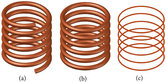
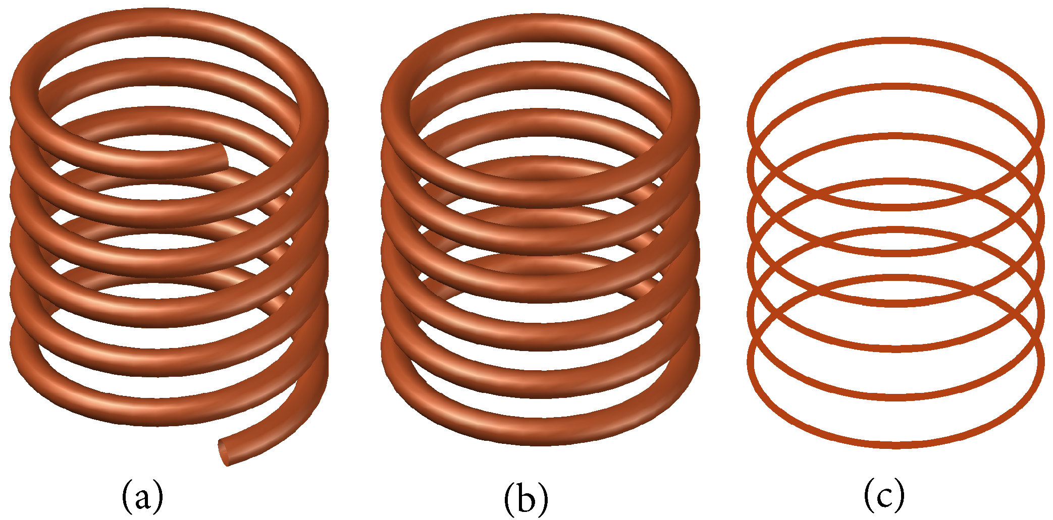
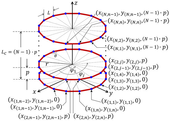
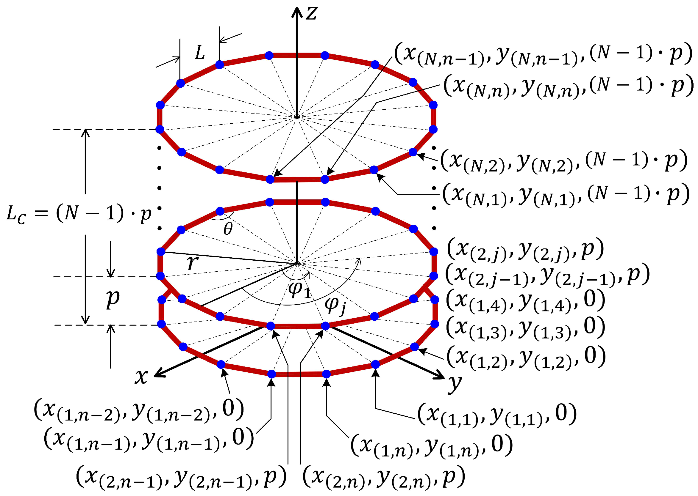
Since the purpose of this work is to calculate the MI between solenoid coils positioned arbitrarily in 3D space, the positions of the solenoid coils in 3D space must first be determined. When modeling circular-wound solenoid coils, the helically wound coils shown in Figure 1a are initially represented as circular turns stacked axially, as in Figure 1b, and are subsequently modeled as filaments equivalent to these circular turns, as shown in Figure 1c. In this approach, each circular turn filament is represented by geometrically equivalent polygonal-turn filament. This method is employed because modeling with circular filaments involves elliptic integrals that are solvable only numerically, whereas the polygonal-turn representation enables an analytical solution. To obtain an analytical solution for the MI between circular-wound solenoid coils arbitrarily positioned in 3D space, the Cartesian coordinates of the vertices of the polygonal turns, which are considered geometrically equivalent to the circular turns, must be known. Figure 2 shows a coil consisting of polygonal-turn filaments stacked axially, which are considered equivalent to a circularly wound helical solenoid coil. This figure also enables the determination of the reference coordinates of the primary and secondary solenoid coils using the filament approach. The coordinates of the vertices of each filament in this coil, along with the number of turns (N), coil length ($L_c$), the turn-to-turn pitch (p) defined as the distance between the centers of two consecutive turns, filament radius (r), side number (n), certain positional angle ($\phi$), polygon angle ($\theta$) are illustrated in the figure. Here, $i,j$ and $k,m$ represent the turn and side index numbers of the filaments corresponding to the primary and secondary, respectively. Furthermore, the subscripts p and s denote the primary and secondary, respectively. After obtaining the angles of the polygonal filaments for the primary (${\theta }_p$) and secondary (${\theta }_s$) using (13), the angles between the filament radius line segment and the x-axis can also be expressed in terms of these parameters by (14).

$$\begin{array}{c}\hfill \begin{array}{cc}\hfill {\theta }_p& =\pi (n_p-2)/n_p\hfill \\ \hfill {\theta }_s& =\pi (n_s-2)/n_s\hfill \end{array}\end{array}$$

(13)

$$\begin{array}{c}\hfill \begin{array}{cc}\hfill {\phi }_{p\left(j\right)}& ={\theta }_p/2+(j-1)(\pi -{\theta }_p)\hfill \\ \hfill {\phi }_{s\left(m\right)}& ={\theta }_s/2+(m-1)(\pi -{\theta }_s)\hfill \end{array}\end{array}$$

(14)

In addition, for an n-sided polygonal filament, the radius can be calculated if the side length is known, or the side length can be calculated if the radius is known by (15). Instead of using the actual circular turn radius of the solenoid coil, an equivalent radius is defined based on the surface enclosed by a single turn. In this context, the radius of a regular polygonal filament enclosing a surface equal to that enclosed by the circular turn is determined, and this equivalent radius is used as the coil radius ($r_p$ and $r_s$) in this study.

$$\begin{array}{c}\hfill \begin{array}{cc}\hfill L_p& =2r_{p}sin({\displaystyle \frac{\pi }{n_p}})\hfill \\ \hfill L_s& =2r_{s}sin({\displaystyle \frac{\pi }{n_s}})\hfill \end{array}\end{array}$$

(15)

Figure 1. Circular-wound solenoid coils (a) helically wound wire, (b) axially stacked circular turns, (c) filamentary representation of the stacked circular turns.

Figure 2. Coordinates, radius, turn-to-turn pitch, angles, coil length and side length representation for modeling circularly wound solenoid coils using multi-sided polygons.

Considering the conductor diameters ($w_p,w_s$) and the spaces between consecutive turns ($s_p,s_s$) for the primary and secondary coils, the distances between the centers of two consecutive turns ($p_p,p_s$) can be expressed by (16).

$$\begin{array}{c}\hfill \begin{array}{cc}\hfill p_p& =w_p+s_p\hfill \\ \hfill p_s& =w_s+s_s\hfill \end{array}\end{array}$$

(16)

The primary and secondary coil lengths ($L_{cp}$, $L_{cs}$) can be calculated by (17). Coil length is defined as the distance between the centers of the first and last turns.

$$\begin{array}{c}\hfill \begin{array}{cc}\hfill L_{cp}& =(N_p-1)·p_p\hfill \\ \hfill L_{cs}& =(N_s-1)·p_s\hfill \end{array}\end{array}$$

(17)

The Cartesian coordinate values of the vertices of the polygonal filaments for the primary and secondary coils are also expressed by (18).

$$\begin{array}{c}\hfill \begin{array}{cc}\hfill x_{p(i,j)}& =r_p\cos \left({\phi }_{p\left(j\right)}\right)\hfill \\ \hfill y_{p(i,j)}& =r_p\sin \left({\phi }_{p\left(j\right)}\right)\hfill \\ \hfill z_{p(i,j)}& =(i-1)p_p\hfill \\ \hfill x_{s(k,m)}& =r_s\cos \left({\phi }_{s\left(m\right)}\right)\hfill \\ \hfill y_{s(k,m)}& =r_s\sin \left({\phi }_{s\left(m\right)}\right)\hfill \\ \hfill z_{s(k,m)}& =(k-1)p_s\hfill \end{array}\end{array}$$

(18)

In this work, since the MI between the primary and secondary solenoid coils is calculated at different positions in 3D space, rotational and translational coordinate transformations are required to determine their relative positions. For angular and lateral misalignment conditions of the coils, rotational and translational coordinate transformations should be employed, respectively. Accordingly, the rotational and translational coordinate transformation equations that enable the determination of the new position coordinates of the primary and secondary coils must be formulated. The new point $P^{\prime }(x^{\prime },y^{\prime },z^{\prime })$ obtained by applying a rotational coordinate transformation to a point $P(x,y,z)$ about any one, two, or all three of the x-, y-, and z-axes, is determined by (19).

$$P^{\prime }(x^{\prime },y^{\prime },z^{\prime })=T(\alpha ,\beta ,\gamma ).P(x,y,z)$$

(19)

where $T(\alpha ,\beta ,\gamma )$ is the rotational transformation matrix derived from the multiplication of $T\left(\alpha \right)$, $T\left(\beta \right)$ and $T\left(\gamma \right)$ matrices given in (20) by considering the Y-X-Z rotation convention. The parameters $\alpha ,\beta$, and $\gamma$ represent the rotation angles of point P about the x-, y-, and z- axes, respectively. This transformation matrix $T(\alpha ,\beta ,\gamma )$ combined from the matrices $T\left(\alpha \right)$, $T\left(\beta \right)$ and $T\left(\gamma \right)$ is formulated as shown in (21).

$$\begin{array}{cc}\hfill T\left(\alpha \right)& =\left(\begin{array}{ccc}1& 0& 0\\ 0& \cos \left(\alpha \right)& -\sin \left(\alpha \right)\\ 0& \sin \left(\alpha \right)& \cos \left(\alpha \right)\end{array}\right)\hfill \\ \hfill T\left(\beta \right)& =\left(\begin{array}{ccc}\cos \left(\beta \right)& 0& \sin \left(\beta \right)\\ 0& 1& 0\\ -\sin \left(\beta \right)& 0& \cos \left(\beta \right)\end{array}\right)\hfill \\ \hfill T\left(\gamma \right)& =\left(\begin{array}{ccc}\cos \left(\gamma \right)& -\sin \left(\gamma \right)& 0\\ \sin \left(\gamma \right)& \cos \left(\gamma \right)& 0\\ 0& 0& 1\end{array}\right)\hfill \end{array}$$

(20)

$$T(\alpha ,\beta ,\gamma )=T\left(\gamma \right).T\left(\alpha \right).T\left(\beta \right)=\left(\begin{array}{ccc}{r}_{11}& r_{12}& r_{13}\\ r_{21}& r_{22}& r_{23}\\ r_{31}& r_{32}& r_{33}\end{array}\right)$$

(21)

In this case, the matrix elements from $r_{11}$ to $r_{33}$, where each element is defined, are given in (22).

$$\begin{array}{c}\hfill \begin{array}{cc}\hfill r_{11}& =\cos \left(\beta \right)\cos \left(\gamma \right)-\sin \left(\alpha \right)\sin \left(\beta \right)\sin \left(\gamma \right)\hfill \\ \hfill r_{12}& =-\cos \left(\alpha \right)\sin \left(\gamma \right)\hfill \\ \hfill r_{13}& =\sin \left(\beta \right)\cos \left(\gamma \right)+\sin \left(\alpha \right)\cos \left(\beta \right)\sin \left(\gamma \right)\hfill \\ \hfill r_{21}& =\cos \left(\beta \right)\sin \left(\gamma \right)+\sin \left(\alpha \right)\sin \left(\beta \right)\cos \left(\gamma \right)\hfill \\ \hfill r_{22}& =\cos \left(\alpha \right)\cos \left(\gamma \right)\hfill \\ \hfill r_{23}& =\sin \left(\beta \right)\sin \left(\gamma \right)-\sin \left(\alpha \right)\cos \left(\beta \right)\cos \left(\gamma \right)\hfill \\ \hfill r_{31}& =-\cos \left(\alpha \right)\sin \left(\beta \right)\hfill \\ \hfill r_{32}& =\sin \left(\alpha \right)\hfill \\ \hfill r_{33}& =\cos \left(\alpha \right)\cos \left(\beta \right)\hfill \end{array}\end{array}$$

(22)

The MI between the primary and secondary coils may need to be calculated under both angular and lateral misalignment conditions. For this purpose, the most general expression that enables the determination of the coils’ new position points is provided in (23).

$$\left(\begin{array}{c}{x}^{\prime }\\ y^{\prime }\\ z^{\prime }\end{array}\right)=\left(\begin{array}{ccc}{r}_{11}& r_{12}& r_{13}\\ r_{21}& r_{22}& r_{23}\\ r_{31}& r_{32}& r_{33}\end{array}\right).\left(\begin{array}{c}x\\ y\\ z\end{array}\right)+\left(\begin{array}{c}\Delta x\\ \Delta y\\ \Delta z\end{array}\right)$$

(23)

where $\Delta x$, $\Delta y$ and $\Delta z$ represent the translational displacements of point P along the x-, y-, and z- axes, respectively. Using the new position determination expression in (23), the solenoid coils in 3D space can have their new positions established under all possible misalignment conditions angular, lateral, and combined angular/lateral allowing the MI between them to be calculated.

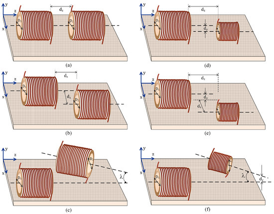
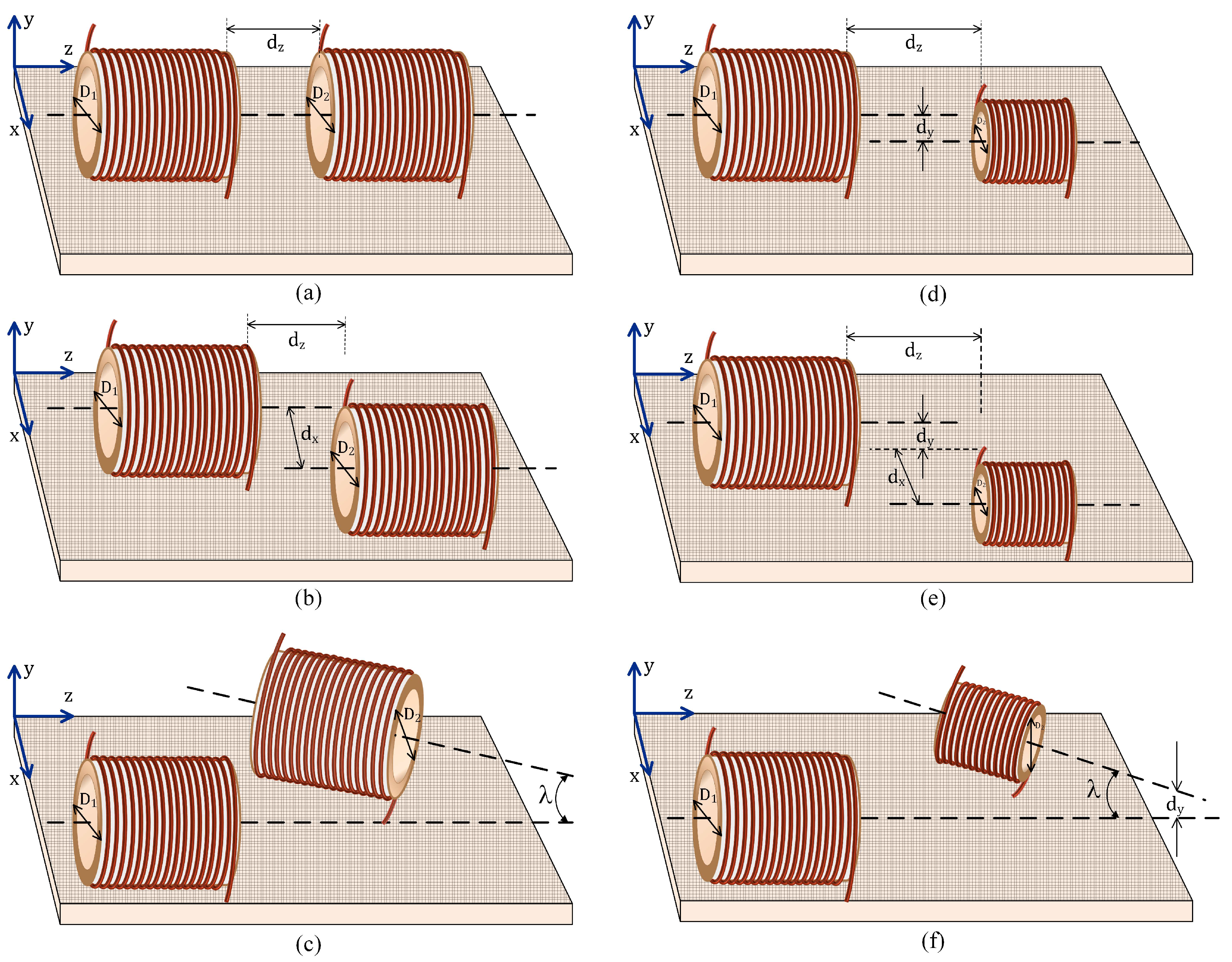
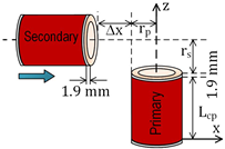
In general, when implementing electrical and electronic systems, one of the essential components required for the system is the coil, and the system is typically placed on a planar surface, with MI occurring between the coils. Accordingly, Figure 3 is presented to consider this situation and illustrate the misalignments between the two coils, where six different configurations are shown. In configurations (a), (b), and (c), the primary and secondary coils have the same diameters, whereas in (d), (e), and (f), the coils have different diameters. In (a), the coils are coaxial with a distance of $d_z$ in the z- direction, while in (b) they are non-coaxial with distances of $d_x$ and $d_z$ in the x- and z- directions, respectively, and in (c) they are non-coaxial with an angular displacement of $\lambda$ between their axes. Similarly, in configurations (d), (e), and (f), since the coil diameters are different, in addition to distances $d_x$ and $d_z$ in the x- and z- directions and the angular displacement $\lambda$, a distance $d_y$ has also occurred.

Figure 3. Spatial positions of two coils on a plane, with equal or unequal diameters: (a) coaxial coils, (b) non-coaxial coils with lateral shift along the x-axis, (c) non-coaxial coils with rotation about the y-axis, (d) non-coaxial coils with lateral shift along the y-axis, (e) non-coaxial coils with lateral shifts along both x- and y-axes, and (f) non-coaxial coils with rotation about the y-axis and lateral shift along the y-axis.

In order to calculate the MI between two circular-wound solenoid coils interacting in 3D space, the MVP formula provided in (10) should be utilized as a preliminary step. Then, the magnetic flux is obtained by performing the integration given in (11) based on the calculated resultant vector of the MVP. The approach presented in this work for calculating the MI between circular-wound solenoid coils is based on modeling the coil turns as multi-sided polygons. In the calculation of MI between direct circularly shaped turns, one encounters elliptic integrals that can only be solved numerically. The MI calculation method based on polygonal-shaped turns used in this work provides an advantage for obtaining an analytical solution, as it involves line segment integrals. Here, while the turns of regular polygon are considered equivalent to circular-shaped turns, it has been deemed sufficient for the polygon to have 36 sides or more in order to accurately approximate the circular geometry.

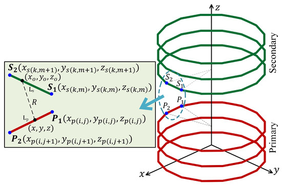
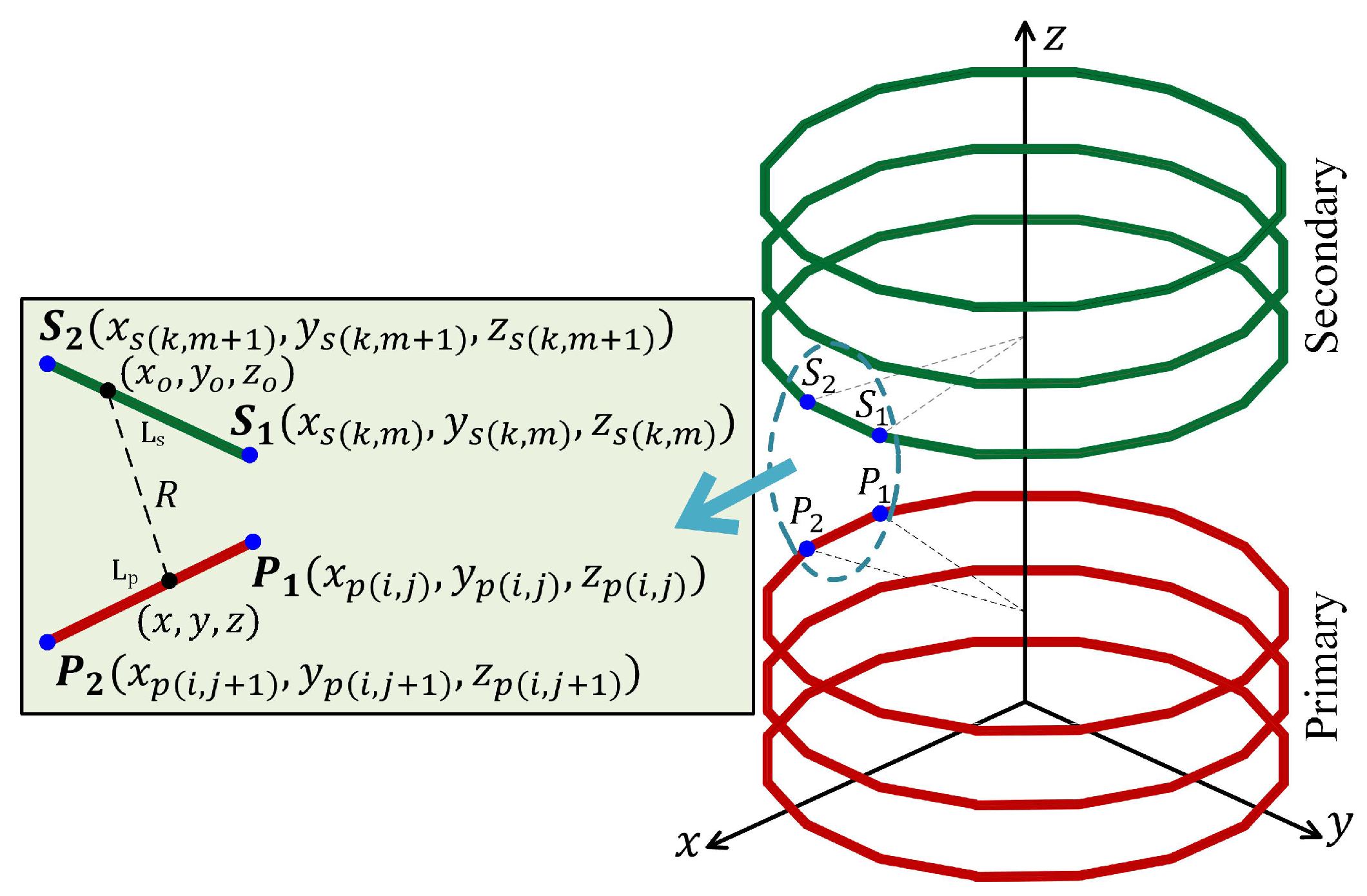
Solenoid-type primary and secondary coils in 3D space, positioned within each other’s magnetic field regions are illustrated in Figure 4. Although the turns are physically implemented as regular polygons, they are assumed to have a sufficient number of sides to be modeled as equivalent to circular turns. Based on the assumption that i,j and k,m represent the turn and side numbers of the primary and secondary coils, respectively, the corner coordinates of the polygonal turns $P_1$-$P_2$ for the primary coil and $S_1$-$S_2$ for the secondary coil are shown in Figure 4. First, it is necessary to calculate the MVP at a point on any side of any turn of the secondary coil due to the current flowing through any side of any turn of primary coil. Therefore, considering that the point $(x,y,z)$ on the primary turn is variable while the point $(x_o,y_o,z_o)$ on the secondary turn is fixed, the MVP at the fixed point $(x_o,y_o,z_o)$ on the side of the secondary coil due to the current in the $L_p$ side of the primary coil can be calculated by substituting $d\overrightarrow{\ell }$ = $d\overrightarrow{{\ell }_p}$ = $dx{\overrightarrow{a}}_x+dy{\overrightarrow{a}}_y+dz{\overrightarrow{a}}_z$ and $R=\sqrt{{(x_o-x)}^2+{(y_o-y)}^2+{(z_o-z)}^2}$ into (10) to obtain (24).

$${\overrightarrow{A}}_{(i,j)}=k_{\mu }{\int }_{L_p}{\displaystyle \frac{dx{\overrightarrow{a}}_x+dy{\overrightarrow{a}}_y+dz{\overrightarrow{a}}_z}{\sqrt{{(x_o-x)}^2+{(y_o-y)}^2+{(z_o-z)}^2}}}$$

(24)

where $k_{\mu }={\mu }_{o}I/4\pi$ and ${\overrightarrow{a}}_x,{\overrightarrow{a}}_y,{\overrightarrow{a}}_z$ are unit vectors in the $x,y,z$ axes directions respectively. Since the integral in (24) is a line integral along a straight segment, it can be solved by parameterization. When solving the line integral along a straight segment, the vector $\overrightarrow{r}\left(t\right)=(1-t){\overrightarrow{r}}_1+t{\overrightarrow{r}}_2$ can be used to parameterize the path, where ${\overrightarrow{r}}_1$ and ${\overrightarrow{r}}_2$ are the position vectors of the segment’s endpoints and t varies from 0 to 1. This representation allows for the integral to be calculated along the straight line connecting ${\overrightarrow{r}}_1$ and ${\overrightarrow{r}}_2$. Therefore, for the path connecting the corner points $P_1$-$P_2$, the coordinates of the variable point $(x,y,z)$ are expressed in terms of the parameter t as in (25).

$$\begin{array}{c}\hfill \begin{array}{cc}\hfill x\left(t\right)& =(1-t).x_{p(i,j)}+t.x_{p(i,j+1)}\hfill \\ \hfill y\left(t\right)& =(1-t).y_{p(i,j)}+t.y_{p(i,j+1)}\hfill \\ \hfill z\left(t\right)& =(1-t).z_{p(i,j)}+t.z_{p(i,j+1)}\hfill \end{array}\end{array}$$

(25)

Taking (26) into account, the differential vector $d{\overrightarrow{\ell }}_p$ can be expressed in terms of the parameter t as in (27).

$$\begin{array}{c}\hfill \begin{array}{cc}\hfill dx& ={\displaystyle \frac{dx}{dt}}dt=x^{\prime }\left(t\right)dt\hfill \\ \hfill dy& ={\displaystyle \frac{dy}{dt}}dt=y^{\prime }\left(t\right)dt\hfill \\ \hfill dz& ={\displaystyle \frac{dz}{dt}}dt=z^{\prime }\left(t\right)dt\hfill \end{array}\end{array}$$

(26)

$$d{\overrightarrow{\ell }}_p=u({\overrightarrow{a}}_x+m_1{\overrightarrow{a}}_y+m_2{\overrightarrow{a}}_z)dt$$

(27)

where u, $m_1$ and $m_2$ are given in (28).

$$\begin{array}{c}\hfill \begin{array}{cc}\hfill u& =x_{p(i,j+1)}-x_{p(i,j)}\hfill \\ \hfill m_1& ={\displaystyle \frac{y_{p(i,j+1)}-y_{p(i,j)}}{x_{p(i,j+1)}-x_{p(i,j)}}}\hfill \\ \hfill m_2& ={\displaystyle \frac{z_{p(i,j+1)}-z_{p(i,j)}}{x_{p(i,j+1)}-x_{p(i,j)}}}\hfill \end{array}\end{array}$$

(28)

After substituting the expressions in (25) and (27) into (24), the single-variable integral equation for calculating the MVP becomes as in (29).

$${\overrightarrow{A}}_{(i,j)}=k_{\mu }{\int }_0^1{\displaystyle \frac{u({\overrightarrow{a}}_x+m_1{\overrightarrow{a}}_y+m_2{\overrightarrow{a}}_z)dt}{\sqrt{U{t}^2+Vt+W}}}$$

(29)

where, the terms U, V and W are defined as in (30).

$$\begin{array}{c}\hfill \begin{array}{cc}\hfill U& =u^2(1+m_1^2+m_2^2)\hfill \\ \hfill V& =-2u(v_1+m_1{v}_2+m_2{v}_3)\hfill \\ \hfill W& =v_1^2+v_2^2+v_3^2\hfill \end{array}\end{array}$$

(30)

The expressions $v_1$, $v_2$ and $v_3$ in V and W of (30) are given in (31).

$$\begin{array}{c}\hfill \begin{array}{cc}\hfill v_1& =x_o-x_{p(i,j)}\hfill \\ \hfill v_2& =y_o-y_{p(i,j)}\hfill \\ \hfill v_3& =z_o-z_{p(i,j)}\hfill \end{array}\end{array}$$

(31)

Solution of the single-variable definite integral in (29) is given in (32).

$$\begin{array}{cc}\hfill & {\overrightarrow{A}}_{(i,j)}=k_{\mu }\ln \left({\displaystyle \frac{\sqrt{U+V+W}+\sqrt{U}+V/2\sqrt{U}}{\sqrt{W}+V/2\sqrt{U}}}\right){\overrightarrow{a}}_A\hfill \end{array}$$

(32)

where the unit vector ${\overrightarrow{a}}_A$ in the direction of the MVP is defined as in (33).

$$\begin{array}{cc}\hfill & {\overrightarrow{a}}_A={\displaystyle \frac{u({\overrightarrow{a}}_x+m_1{\overrightarrow{a}}_y+m_2{\overrightarrow{a}}_z)}{\left|u\right|\sqrt{1+m_1^2+m_2^2}}}\hfill \end{array}$$

(33)

Figure 4. Solenoid-type primary and secondary coils in 3D space.

The result in (32) represents the MVP at a point on any side of any turn of secondary coil due to the current flowing through any side of any turn of the polygonal primary coil, with both coils considered equivalent to circular-wound solenoids. The MI between the two solenoid coils can be determined by substituting this vector expression into (11) and calculating the magnetic flux. To calculate the magnetic flux passing through the surface enclosed by any turn of the secondary coil using this MVP vector, the coordinates of the point $x_o,y_o,z_o$ on the side of the secondary turn, which were previously considered fixed, must now be treated as variables. Therefore, by substituting (31) into (30) and replacing $x_o$, $y_o$ and $z_o$ with x, y, and z respectively, (34) is obtained from (32).

$$\begin{array}{cc}\hfill & {\overrightarrow{A}}_{(i,j)}=k_{\mu }\ln \left({\displaystyle \frac{\sqrt{{(x-x_{p(i,j+1)})}^2+{(y-y_{p(i,j+1)})}^2+{(z-z_{p(i,j+1)})}^2}+\frac{u^2(1+m_1^2+m_2^2)-u((x-x_{p(i,j)})+m_1(y-y_{p(i,j)})+m_2(z-z_{p(i,j)}))}{\left|u\right|\sqrt{1+m_1^2+m_2^2}}}{\sqrt{{(x-x_{p(i,j)})}^2+{(y-y_{p(i,j)})}^2+{(z-z_{p(i,j)})}^2}-\frac{u((x-x_{p(i,j)})+m_1(y-y_{p(i,j)})+m_2(z-z_{p(i,j)}))}{\left|u\right|\sqrt{1+m_1^2+m_2^2}}}}\right){\overrightarrow{a}}_A\hfill \end{array}$$

(34)

The MVP vector with variables x, y, and z from (34) can be used to calculate the line integral along the path between the corner points $S_1$ and $S_2$ in Figure 4. Since the path connecting $S_1$ to $S_2$ is also a straight line segment, by parametrizing $\overrightarrow{r}\left(t\right)=(1-t){\overrightarrow{r}}_3+t{\overrightarrow{r}}_4$, the MVP vector in x, y, and z is expressed as a function of single variable t, allowing the magnetic flux in (11) to be obtained by using (35). Here, ${\overrightarrow{r}}_3$ is the position vector of point $S_1$, ${\overrightarrow{r}}_4$ is the position vector of point $S_2$, and t varies from 0 to 1. $L_s$ is the line segment connecting ${\overrightarrow{r}}_3$ and ${\overrightarrow{r}}_4$.

$$\begin{array}{cc}\hfill {\varphi }_{(i,j,k,m)}& ={\int }_{L_s}{\overrightarrow{A}}_{(i,j)}·d{\overrightarrow{\ell }}_s\hfill \end{array}$$

(35)

where $d{\overrightarrow{\ell }}_s$ = $dx{\overrightarrow{a}}_x+dy{\overrightarrow{a}}_y+d{\overrightarrow{a}}_z$. Following a parametrization analogous to the one previously employed, the parametrization equations for the new variables $x,y,z$ can be formulated in the same way as in (36).

$$\begin{array}{c}\hfill \begin{array}{cc}\hfill x\left(t\right)& =(1-t).x_{s(k,m)}+t.x_{s(k,m+1)}\hfill \\ \hfill y\left(t\right)& =(1-t).y_{s(k,m)}+t.y_{s(k,m+1)}\hfill \\ \hfill z\left(t\right)& =(1-t).z_{s(k,m)}+t.z_{s(k,m+1)}\hfill \end{array}\end{array}$$

(36)

Considering (26), the vector $d{\overrightarrow{\ell }}_s$ can be expressed as given in (37).

$$d{\overrightarrow{\ell }}_s=v({\overrightarrow{a}}_x+m_3{\overrightarrow{a}}_y+m_4{\overrightarrow{a}}_z)dt$$

(37)

where v, $m_3$ and $m_4$ are given in (38).

$$\begin{array}{c}\hfill \begin{array}{cc}\hfill v& =x_{s(k,m+1)}-x_{s(k,m)}\hfill \\ \hfill m_3& ={\displaystyle \frac{y_{s(k,m+1)}-y_{s(k,m)}}{x_{s(k,m+1)}-x_{s(k,m)}}}\hfill \\ \hfill m_4& ={\displaystyle \frac{z_{s(k,m+1)}-z_{s(k,m)}}{x_{s(k,m+1)}-x_{s(k,m)}}}\hfill \end{array}\end{array}$$

(38)

If the expression in (37) is substituted into (35), (39) is obtained.

$${\varphi }_{(i,j,k,m)}=v{\int }_0^1{\overrightarrow{A}}_{(i,j)}·({\overrightarrow{a}}_x+m_3{\overrightarrow{a}}_y+m_4{\overrightarrow{a}}_z)dt$$

(39)

After substituting the MVP vector in (34) into (39) and performing some necessary algebraic operations, the magnetic flux equation can be expressed as in (40).

$${\varphi }_{(i,j,k,m)}=-k_{\mu }{a}_5{\int }_0^1\ln \left({\displaystyle \frac{\sqrt{a_1{t}^2+a_{2}t+a_3}+a_4+a_{5}t}{\sqrt{b_1{t}^2+b_{2}t+b_3}+b_4+b_{5}t}}\right)dt$$

(40)

where $a_1,a_2,a_3,a_4,a_5$ and $b_1,b_2,b_3,b_4,b_5$ are given in (41) and (42) respectively.

$$\begin{array}{c}\hfill \begin{array}{cc}\hfill a_1=& v^2(1+m_3^2+m_4^2)\hfill \\ \hfill a_2=& 2v[(x_{s(k,m)}-x_{p(i,j+1)})+m_3(y_{s(k,m)}-y_{p(i,j+1)})+m_4(z_{s(k,m)}-z_{p(i,j+1)})]\hfill \\ \hfill a_3=& {(x_{s(k,m)}-x_{p(i,j+1)})}^2+{(y_{s(k,m)}-y_{p(i,j+1)})}^2+{(z_{s(k,m)}-z_{p(i,j+1)})}^2\hfill \\ \hfill a_4=& \left[u^2(1+m_1^2+m_2^2)-u[(x_{s(k,m)}-x_{p(i,j)})+m_1(y_{s(k,m)}-y_{p(i,j)})+m_2(z_{s(k,m)}-z_{p(i,j)})]\right]/\hfill \\ \hfill & \left|u\right|\sqrt{1+m_1^2+m_2^2}\hfill \\ \hfill a_5=& {\displaystyle \frac{-uv(1+m_1{m}_3+m_2{m}_4)}{\left|u\right|\sqrt{1+m_1^2+m_2^2}}}\hfill \end{array}\end{array}$$

(41)

$$\begin{array}{c}\hfill \begin{array}{cc}\hfill b_1=& v^2(1+m_3^2+m_4^2)\hfill \\ \hfill b_2=& 2v[(x_{s(k,m)}-x_{p(i,j)})+m_3(y_{s(k,m)}-y_{p(i,j)})+m_4(z_{s(k,m)}-z_{p(i,j)})]\hfill \\ \hfill b_3=& {(x_{s(k,m)}-x_{p(i,j)})}^2+{(y_{s(k,m)}-y_{p(i,j)})}^2+{(z_{s(k,m)}-z_{p(i,j)})}^2\hfill \\ \hfill b_4=& \left[-u[(x_{s(k,m)}-x_{p(i,j)})+m_1(y_{s(k,m)}-y_{p(i,j)})+m_2(z_{s(k,m)}-z_{p(i,j)})]\right]/\hfill \\ & \left|u\right|\sqrt{1+m_1^2+m_2^2}\hfill \\ \hfill b_5=& {\displaystyle \frac{-uv(1+m_1{m}_3+m_2{m}_4)}{\left|u\right|\sqrt{1+m_1^2+m_2^2}}}\hfill \end{array}\end{array}$$

(42)

The analytical solution of the integral expression given in (40) requires nontrivial calculations and is based on Euler’s second substitution method. The explicit solution will not be presented here, as it has already been derived in our previous study [28]. In that study, following the variable transformation procedures, the integral expression was transformed into an analytically solvable form through a series of algebraic manipulations and integral transformations. The fundamental mathematical structure and implementation procedure of the related integral solution approach were therefore presented in detail. Since an expansion of the solution function $F_1(t;(a_1,a_2,a_3,a_4,a_5))$ corresponding to the integral given in (43) is available, the expansion of the solution function $F_2(t;(b_1,b_2,b_3,b_4,b_5))$ equals to the integral of the form $\int ln(\sqrt{b_1{t}^2+b_{2}t+b_3}+b_4+b_{5}t)$ can be obtained directly.

$$\begin{array}{c}\hfill \begin{array}{cc}\hfill F_1& \left(t;(a_1,a_2,a_3,a_4,a_5)\right)=\int \ln \left(\sqrt{a_1{t}^2+a_{2}t+a_3}+a_4+a_{5}t\right)dt\hfill \\ \hfill =& -t+\left(t-{\displaystyle \frac{a_2-2a_5{a}_4}{2(a_5^2-a_1)}}\right)\ln \left(\sqrt{a_1{t}^2+a_{2}t+a_3}+a_4+a_{5}t\right)\hfill \\ \hfill & +{\displaystyle \frac{a_5{a}_2-2a_1{a}_4}{\sqrt{a_1}(a_5^2-a_1)}}\mathrm{arccoth}\left({\displaystyle \frac{\sqrt{a_1{t}^2+a_{2}t+a_3}-\sqrt{a_3}}{\sqrt{a_1}t}}\right)\hfill \\ & +{\displaystyle \frac{\sqrt{4(a_5^2-a_1)(a_4^2-a_3)-{(a_2-2a_5{a}_4)}^2}}{a_5^2-a_1}}\hfill \\ & \times \arctan [\sqrt{{\displaystyle \frac{a_5{a}_2-a_1(a_4+\sqrt{a_3})}{a_4-\sqrt{a_3}}}-{\left({\displaystyle \frac{a_2-2a_5\sqrt{a_3}}{2(a_4-\sqrt{a_3})}}\right)}^2}/\hfill \\ & \left({\displaystyle \frac{\sqrt{a_1{t}^2+a_{2}t+a_3}-\sqrt{a_3}}{t}}+{\displaystyle \frac{a_2-2a_5\sqrt{a_3}}{2(a_4-\sqrt{a_3})}}\right)]\hfill \end{array}\end{array}$$

(43)

Since the expansions of the solution functions $F_1$ and $F_2$ are now known, (44) can be employed to obtain the magnetic flux ${\varphi }_{(i,j,k,m)}$.

$$\begin{array}{cc}\hfill {\varphi }_{(i,j,k,m)}=& -k_{\mu }{a}_5\left[F_1(t;(a_1,a_2,a_3,a_4,a_5)){|}_0^1-F_2(t;(b_1,b_2,b_3,b_4,b_5)){|}_0^1\right]\hfill \end{array}$$

(44)

As can be seen from (44), if (t = 0) is substituted into the solution function, it becomes evident that in the explicit expression given in (43), the $(\sqrt{a_1{t}^2+a_{2}t+a_3}-\sqrt{a_3})/\sqrt{a_1}t$ and $(\sqrt{a_1{t}^2+a_{2}t+a_3}-\sqrt{a_3})/t$ lead to indeterminate forms. For the term $(\sqrt{a_1{t}^2+a_{2}t+a_3}-\sqrt{a_3})/\sqrt{a_1}t$, when the limit is evaluated as t→0, the result is $a_2/\left(2\sqrt{a_1{a}_3}\right)$. For the term $(\sqrt{a_1{t}^2+a_{2}t+a_3}-\sqrt{a_3})/t$, when the limit is evaluated as t→0, the result is $a_2/\left(2\sqrt{a_3}\right)$. Accordingly, any potential indeterminacy in the calculations arising from these terms is thereby eliminated.

The magnetic flux contribution through the (m-$th$) side of the (k-$th$) turn of a regular polygonal filament, which is equivalent to a circular-wound turn of the solenoid secondary coil, can now be calculated. This contribution arises from the current flowing through the (j-$th$) side of the (i-$th$) turn of the regular polygonal filament, equivalent to a circular-wound turn of the solenoid primary coil. Once these contribution is known, the total magnetic flux linking all turns of the secondary coil due to all turns of the primary coil can be determined. From this total flux linkage, the MI can then be obtained. When the total flux is calculated, it is assumed that the primary coil has $N_p$ turns, each with $n_p$ sides, and similarly, the secondary coil has $N_s$ turns, each with $n_s$ sides. In this case, to obtain the MI using (1), the calculation for ${\varphi }_{(i,j,k,m)}$ must be repeated ($N_p\times n_p\times N_s\times n_s$) times. Subsequently, the MI can be determined using (45).

$$\begin{array}{c}\hfill M={\displaystyle \frac{1}{I}}{\displaystyle \sum _{i=1}^{N_p}}{\displaystyle \sum _{j=1}^{n_p}}{\displaystyle \sum _{k=1}^{N_s}}{\displaystyle \sum _{m=1}^{n_s}}{\varphi }_{(i,j,k,m)}\end{array}$$

(45)

In order to avoid special geometrical cases causing singularities, very small angular perturbations were applied to the initial positions of the coils around the z-axis. In this context, the primary and secondary coils were rotated around the z-axis by $0.1°$ and $0.11°$, respectively, resulting in a relative angular error of ($0.01°$). The effect of these very small angular perturbations on the MI results remains at a negligible level [28].

3. Performance Analysis of the MI Calculation Model

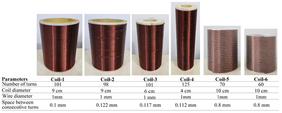
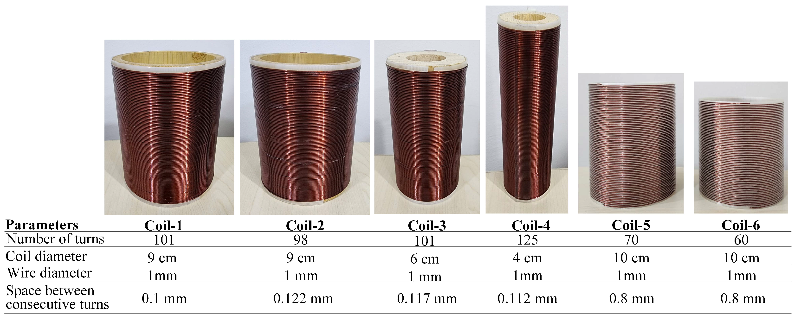
Based on the calculation approach introduced in Section 2, this section evaluates the performance and applicability of the proposed MI calculation model through several complementary analyses. First, the convergence behavior of the polygonal representation used for circular-wound solenoid coils is examined by considering different geometrical definitions and different numbers of polygon sides. Then, the accuracy of the proposed formulation is verified using benchmark cases available in the literature for coaxial solenoid configurations. In addition to these validation studies, 3D plots of the MI and MVP are presented for coil arrangements with various angular and/or lateral positions in order to illustrate the spatial behavior of the proposed model.To demonstrate the performance of the analytical approach developed in this work, six coils with different characteristics in terms of size were employed. The images of the coils and their dimensional parameters are shown in Figure 5. Table 2 presents six different coil systems formed from these six coils.

Figure 5. Coils used in this work and their design parameters.

Table 2. Coil Systems formed from the coils of Figure 5.

Coil System	Primary Coil	Secondary Coil
CS-99	Coil-2	Coil-1
CS-66	Coil-3	Coil-3
CS-44	Coil-4	Coil-4
CS-96	Coil-1	Coil-3
CS-94	Coil-1	Coil-4
CS-1010	Coil-5	Coil-6

In the proposed analytical model, the circular-wound solenoid coils are represented by successive circular filamentary turns distributed along the coil axis. Each circular filamentary turn is approximated by an equivalent regular polygon with a sufficient number of sides. This representation enables the MVP and the magnetic flux linked with the secondary coil to be calculated through analytical line integrals over finite straight-line segments. However, the number of sides used in the equivalent polygonal representation must be properly selected in order to approximate the circular filament with sufficient accuracy. This is because the number of sides directly affects both the geometrical accuracy of the circular-turn approximation and the computational load of the analytical model. For polygonal coils to converge to circular coils in terms of MI results, one of the basic geometrical quantities of the polygon must be kept equal to the corresponding quantity of the circular coil while increasing the number of sides. In this context, the enclosed surface, turn circumference, or radius of the polygon can be defined to be identical to that of the corresponding circular coil [29]. In this work, in order to evaluate the accuracy of the 36-sided polygonal representation for the present circular-wound solenoid problem, convergence analyses were performed for both coaxial and misaligned solenoid coil configurations. In the first stage of the convergence analysis, the CS-1010 coil system, whose geometrical parameters and configuration are given in Figure 5 and Table 2, respectively, was considered in a coaxial arrangement. In this case, the primary and secondary solenoid coils were aligned along a common central axis, and the convergence analysis was performed for two axial distances of 15 cm and $15.42$ cm. Here, the axial distance is defined as the distance measured along the common central axis from the lower end plane of the primary coil to the lower end plane of the secondary coil. The number of sides used in the equivalent polygonal representation of the circular filaments was then gradually increased to evaluate the convergence behavior of the MI values. This analysis was performed under three different geometrical definitions: the constant radius (CR), constant enclosed surface (CES), and constant turn circumference (CTC) approaches. In these approaches, the polygon radius, enclosed surface, and turn circumference were separately kept equal to those of the corresponding circular filament. The MI values and the corresponding elapsed times obtained for different numbers of sides and axial distances are presented in Table 3.

Table 3. Convergence of MI and elapsed time with respect to the polygon side number for the coaxial CS-1010 coil system at different axial distances.

Sides Number	z (cm)	M (µH) (CR)	Elapsed Time (s)	M (µH) (CES)	Elapsed Time (s)	M (µH) (CTC)	Elapsed Time (s)
12	15	21.23896316	0.779	22.76137464	0.831	21.98271612	0.767
18	15	22.07955004	1.625	22.76483590	1.653	22.41872539	1.612
24	15	22.37823418	2.700	22.76540930	2.727	22.57072219	2.743
36	15	22.59300292	5.795	22.76562052	5.770	22.67909421	5.862
50	15	22.67606547	10.941	22.76558439	11.017	22.72080354	10.955
100	15	22.74325157	42.903	22.76567132	43.491	22.75445776	42.713
150	15	22.75570597	95.208	22.76567203	96.629	22.76068849	95.737
200	15	22.76006571	166.432	22.76567225	165.615	22.76286895	168.492
12	15.42	19.28816484	0.762	20.69817692	0.810	19.97678220	0.805
18	15.42	20.06621588	1.629	20.70112234	1.675	20.38041187	1.639
24	15.42	20.34285493	2.753	20.70160961	2.720	20.52119925	2.689
36	15.42	20.54182858	5.661	20.70178906	5.832	20.62160444	5.721
50	15.42	20.61879488	11.051	20.70182136	10.997	20.66025321	10.792
100	15.42	20.68105521	42.225	20.70183223	42.325	20.69144017	42.139
150	15.42	20.69259707	94.305	20.70183287	94.239	20.69721438	94.778
200	15.42	20.69663741	169.288	20.70183304	168.433	20.69923521	166.820

As can be seen from the results presented in Table 3, the MI values obtained under the three different geometrical definitions converge to nearly the same value as the number of sides increases. However, the CES approach provides faster convergence to the circular-turn equivalent compared with the other two approaches. In particular, for the 36-sided polygonal representation, the MI values obtained using the CES approach are almost identical to those obtained from the 200-sided polygonal representation. In the error evaluation, the 200-sided polygonal representation was taken as the reference, and the relative difference was calculated as $\epsilon =100·|M_{200}-M_{36}|/M_{200}$. As can be seen from Table 3, under the CES approach, the relative errors between the MI values obtained using the 36-sided and 200-sided representations are approximately $0.00023\%$ and $0.00021\%$ for $z=15$ cm and $z=15.42$ cm, respectively. These very small differences indicate that the 36-sided polygonal representation provides sufficient geometrical accuracy for the circular-turn approximation.

The convergence behavior of the polygonal representation was also examined under misaligned configurations. For this purpose, three representative cases were considered: lateral misalignment, angular misalignment, and lateral-angular misalignment to the secondary coil, while the primary coil was kept fixed at the origin of the base center. For each configuration, the number of sides used in the equivalent polygonal representation of the circular filaments was increased, and the corresponding MI values and elapsed times were calculated using the CR, CES, and CTC approaches. The obtained results are presented in Table 4, where the CES approach is observed to provide the fastest convergence among the considered approaches. Considering the 200-sided representation as the reference, the relative errors of the 36-sided representation are approximately $0.000039\%$, $0.000218\%$, and $0.000016\%$ for the lateral, angular, and lateral-angular misalignment cases, respectively. Therefore, the error introduced by using 36 sides is negligible for all investigated misaligned configurations.These results indicate that when the enclosed surface of the polygon is kept equal to that of the corresponding circular turn, the 36-sided polygonal representation provides very high accuracy for both coaxial and misaligned solenoid configurations. On the other hand, increasing the number of sides from 36 to 200 provides only a negligible improvement in the MI values, while increasing the elapsed time by approximately 29 times. Therefore, in this work, the use of 36-sided regular polygonal filaments based on the CES approach was considered an appropriate choice for representing circular solenoid turns in terms of both accuracy and computational cost.

Table 4. Convergence of MI and elapsed time with respect to the polygon side number for different misaligned CS-1010 coil system.

Sides Number	M (µH) (CR)	Elapsed Time (s)	M (µH) (CES)	Elapsed Time (s)	M (µH) (CTC)	Elapsed Time (s)
Lateral misalignment: $x=5\mathrm{cm}$, $y=5\mathrm{cm}$, $z=15.42\mathrm{cm}$
12	8.78199622	0.810	9.61935185	0.803	9.18891409	0.795
18	9.24059423	1.608	9.61960860	1.607	9.42775438	1.654
24	9.40509697	2.626	9.61965195	2.733	9.51162922	2.695
36	9.52387711	5.809	9.61966801	5.815	9.57162487	5.825
50	9.56992641	10.936	9.61967088	10.837	9.59475877	10.901
100	9.60721817	42.006	9.61967183	41.913	9.61344252	42.673
150	9.61413546	95.688	9.61967179	95.550	9.61690318	96.851
200	9.61655737	168.776	9.61967180	168.362	9.61811440	169.228
Angular misalignment: $\alpha =15°$, $z=15.42\mathrm{cm}$
12	19.66461673	0.781	21.11068205	0.800	20.37074431	0.747
18	20.46251516	1.670	21.11375631	1.674	20.78477515	1.611
24	20.74626199	2.700	21.11426647	2.746	20.92919858	2.745
36	20.95036347	5.621	21.11445458	5.799	21.03219821	5.715
50	21.02931691	10.536	21.11448829	10.917	21.07184591	10.785
100	21.09318853	42.160	21.11449988	43.206	21.10383916	42.983
150	21.10502568	94.867	21.11450050	94.349	21.10976239	94.741
200	21.10917067	168.066	21.11450060	168.310	21.11183541	168.377
Lateral and angular misalignment: $x=5\mathrm{cm}$, $y=5\mathrm{cm}$, $z=15.42\mathrm{cm}$, $\alpha =15°$
12	8.87984027	0.799	9.75994775	0.813	9.30724425	0.786
18	9.36135131	1.648	9.76000820	1.672	9.55815409	1.612
24	9.53429552	2.700	9.76002576	2.685	9.64635859	2.729
36	9.65923416	5.782	9.76003187	5.815	9.70947418	5.759
50	9.70768477	10.587	9.76003298	10.782	9.73381614	10.958
100	9.74692718	42.966	9.76003336	43.113	9.75347760	42.778
150	9.75420684	95.505	9.76003338	96.373	9.75711958	95.377
200	9.75675564	170.821	9.76003339	169.507	9.75839435	168.978

To further validate the proposed analytical model for coaxial solenoid configurations, additional comparisons were performed using established classical benchmark results reported in the literature. As presented in Table 5, the MI values obtained using the proposed model are in very good agreement with the benchmark results reported.

Table 5. Comparison of the analytical model results with classical benchmark results in the literature for coaxial solenoid configurations.

Parameters							Benchmark	Reported	This
${\mathit{r}}_{\mathit{p}}$ (cm)	${\mathit{r}}_{\mathit{s}}$ (cm)	${\mathit{L}}_{\mathit{cp}}$ (cm)	${\mathit{L}}_{\mathit{cs}}$ (cm)	${\mathit{N}}_{\mathit{p}}$	${\mathit{N}}_{\mathit{s}}$	$\mathit{z}$ (cm)	Source	MI	Work
10	5	200	200	2000	2000	0	Maxwell, Cohen [18]	18.808 mH	18.808 mH
5	4	30	5	300	200	12.5	Roiti, Searle and Airey [18]	1.199 mH	1.199 mH
5	2	30	24	300	960	3	Roiti, Searle and Airey [18]	1.370 mH	1.370 mH
3	2	6	10	60	100	16	Dwight and Grover [19]	850.22 nH	850.163 nH

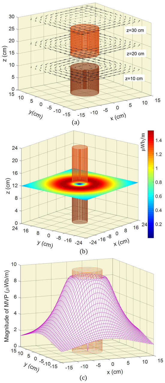
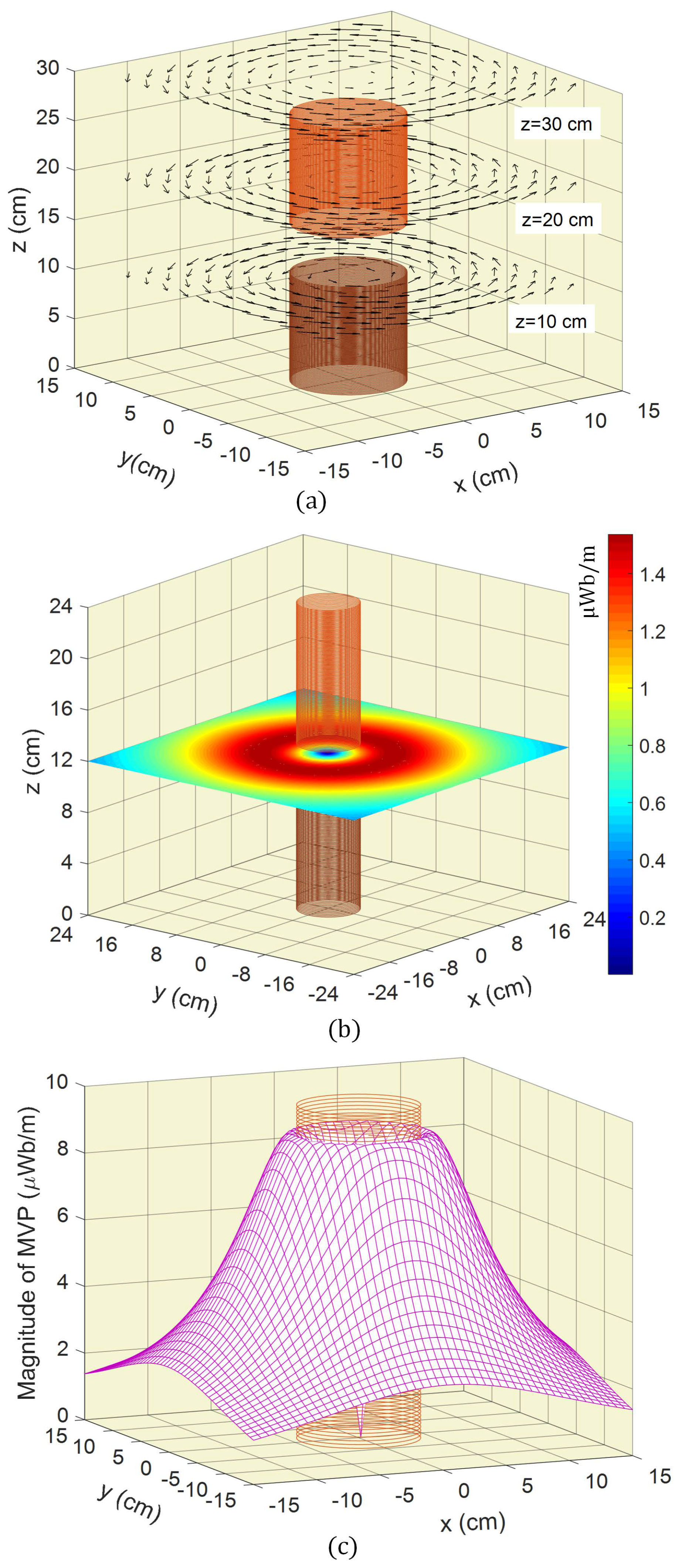
In the analytical model, since the MVP is employed to calculate the magnetic flux for determining the MI, the field distribution of the MVP in 3D space is illustrated in Figure 6. In Figure 6a, the vector field distribution of the MVP on the planes z = 10 cm, z = 20 cm, and z = 30 cm generated by a 1 A current flowing through the primary coil of the CS-99 coil system is presented. As expected, the magnitude of the MVP increases from zero as one moves in the direction perpendicular to the axis passing through the center of the coil, reaching a maximum toward the edge of the coil. Figure 6b shows the distribution of the MVP magnitude on the plane z = 12 cm generated by the current flowing through the primary coil, where the field is color-mapped according to its intensity. As observed, the region with high MVP values is concentrated along the coil edge. Figure 6c presents the 3D plot of the MVP field intensity on the plane z = 4 cm. As observed from this plot, on the plane, when moving in the direction perpendicular to the coil’s central axis, the MVP increases from zero up to the coil edge. Beyond the coil edge, the MVP magnitude decreases as the distance from the center continues to increase. Prior to presenting the MI results, these figures are included to clarify how the secondary coil is affected by the MVP generated by the primary coil, particularly under misalignment conditions. Variations in the geometric parameters and relative positioning of the coils lead to corresponding changes in the profiles of the MI curves. Hence, for a proper interpretation of these graphical results, it is crucial to examine both the spatial distribution of the MVP and its magnitude variation at arbitrary points within the 3D space.

Figure 6. For the coil system, CS-99: (a) MVP field distributions at z = 10, 20 and 30 cm (b) coil geometry and MVP color map at z = 12 cm, and (c) 3D MVP plots at z = 4 cm.

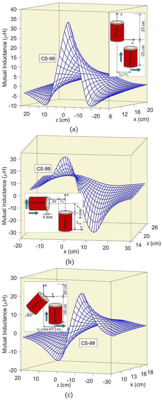
The 3D plots for the CS-99 coil system under lateral and angular misalignment conditions are presented in Figure 7 to demonstrate the effectiveness of the proposed MI calculation model. As shown in Figure 7a, the primary coil is fixed at the origin of the base center, while the secondary coil is shifted along the x-axis in 1 cm increments. For each 1 cm step along the x-axis, the coil is moved along the z-axis from −25 cm to 25 cm in 1 cm increments. The MI was calculated for each position, and the results are presented in a 3D plot. As expected, the MI decreases as the displacement along the x-axis increases due to the weakening of the magnetic coupling between the coils. The plot in Figure 7b was obtained with the primary coil fixed at the origin of the base center. The secondary coil was rotated $90°$ about the y-axis and then positioned along the z-axis in 1 cm increments, and along the x-axis within the range [−17, 29] cm, also in 1 cm steps. The MI was calculated for each position. As shown in the figure, the MI decreases as the secondary coil moves along the z-axis, since it gradually moves away from the magnetic field influence of the primary coil. Figure 7c presents the 3D distribution of MI with the primary and secondary coils oriented at a $45°$ angular displacement between their axes. The secondary coil was incrementally displaced along the z-axis from −30 cm to 20 cm in 1 cm steps and along the x-axis also in 1 cm increments. The MI was calculated for each discrete coil position. As observed, the MI decreases as the secondary coil moves away from the primary coil along both axes, reflecting the attenuation of magnetic coupling due to increased spatial separation.

Figure 7. 3D plots of MI variation for various displacements of the secondary coil for the coil system, CS-99: (a) lateral and (b,c) both angular and lateral misalignment.

4. Model Verification and Experimental Results

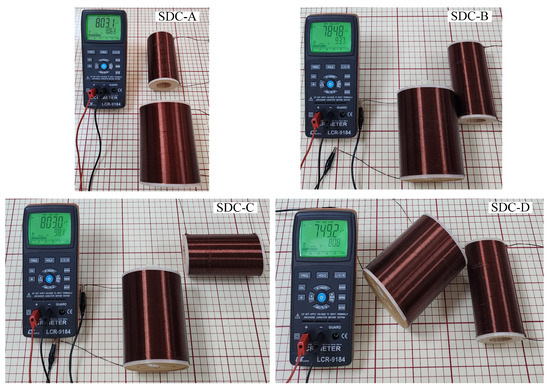
The analytical model developed in this work facilitates the precise determination of MI through a unified closed-form analytical expression, even when the solenoidal primary and secondary windings are arbitrarily oriented and laterally displaced with respect to each other in 3D space. The experimental validation of the MI calculation model under angular and lateral misalignment conditions is carried out using four different spatial displacement configurations (SDC), as shown in Figure 8. For each measurement configuration, results are obtained for the six coil systems listed in Table 2.

Figure 8. Experimental measurement setups for spatial displacement configurations: SDC-A, SDC-B, SDC-C and SDC-D.

The MI was experimentally measured using an LCR meter (Lutron LCR-9184) at a measurement frequency of 100 kHz. The experimental measurement platform was constructed using a scaled planar reference surface, in which each square region has dimensions of $1\mathrm{cm}\times 1\mathrm{cm}$. This arrangement enabled controlled and repeatable positioning of the coils during the measurements. MI cannot be measured directly; therefore, a two-step measurement procedure was applied for each two-coil connection. In the first step, the primary and secondary coils were connected with additive polarity, and the measured inductance was recorded as $L_1$, which is expressed as $L_1=L_{\mathrm{pri}}+L_{\sec }+2M$. In the second step, the coils were connected with subtractive polarity, and the measured inductance was recorded as $L_2$, which is expressed as $L_2=L_{\mathrm{pri}}+L_{\sec }-2M$. Here, $L_{\mathrm{pri}}$ and $L_{\sec }$ denote the self-inductances of the primary and secondary coils, respectively, and M represents the MI between the two coils. The MI can then be indirectly calculated using $(L_1-L_2)/4$. A test frequency of 100 kHz was selected to increase the inductive reactance and improve the sensitivity of the MI measurements. The proposed analytical formulation is based on magnetostatic assumptions, in which the conductors are represented as filamentary current paths. Furthermore, single-layer air-core solenoid coil structures were considered in this study. Since the physical dimensions of the coils are much smaller than the electromagnetic wavelength at 100 kHz, the experimental system can be considered to operate under magneto-quasi-static conditions, and wave propagation effects can be neglected. Under these conditions, the effects of parasitic capacitances and other high-frequency electromagnetic phenomena are expected to remain limited at the selected measurement frequency. Therefore, the selected measurement frequency is considered compatible with the assumptions of the proposed analytical model [20,30].

For comparison of the analytical results of this work with finite element method (FEM) results, 3D models of the CS-99, CS-66, CS-44, CS-96, CS-94, and CS-1010 coil systems were created in Ansys Maxwell 3D. In the FEM analyses of the CS-99, CS-66, CS-44, CS-96, and CS-94 coil systems, the coil windings were represented by equivalent homogenized winding regions instead of directly modeling each helical conductor turn. The equivalent winding region was defined using the inner radius, outer radius, axial length, and number of turns of each solenoid. This representation was adopted to reduce the computational cost of the FEM simulations for tightly wound high-turn solenoids. For the CS-1010 coil system, a helical conductor representation was generated in Ansys Maxwell 3D using the SegmentedHelix/PolygonHelix approach, so that each conductor follows the helical winding path of the primary and secondary coils. The FEM analyses were performed in Ansys Maxwell 3D using the magnetostatic solver. Current excitation was applied in the simulations, and a length-based mesh assignment was used.

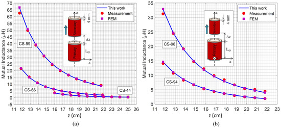
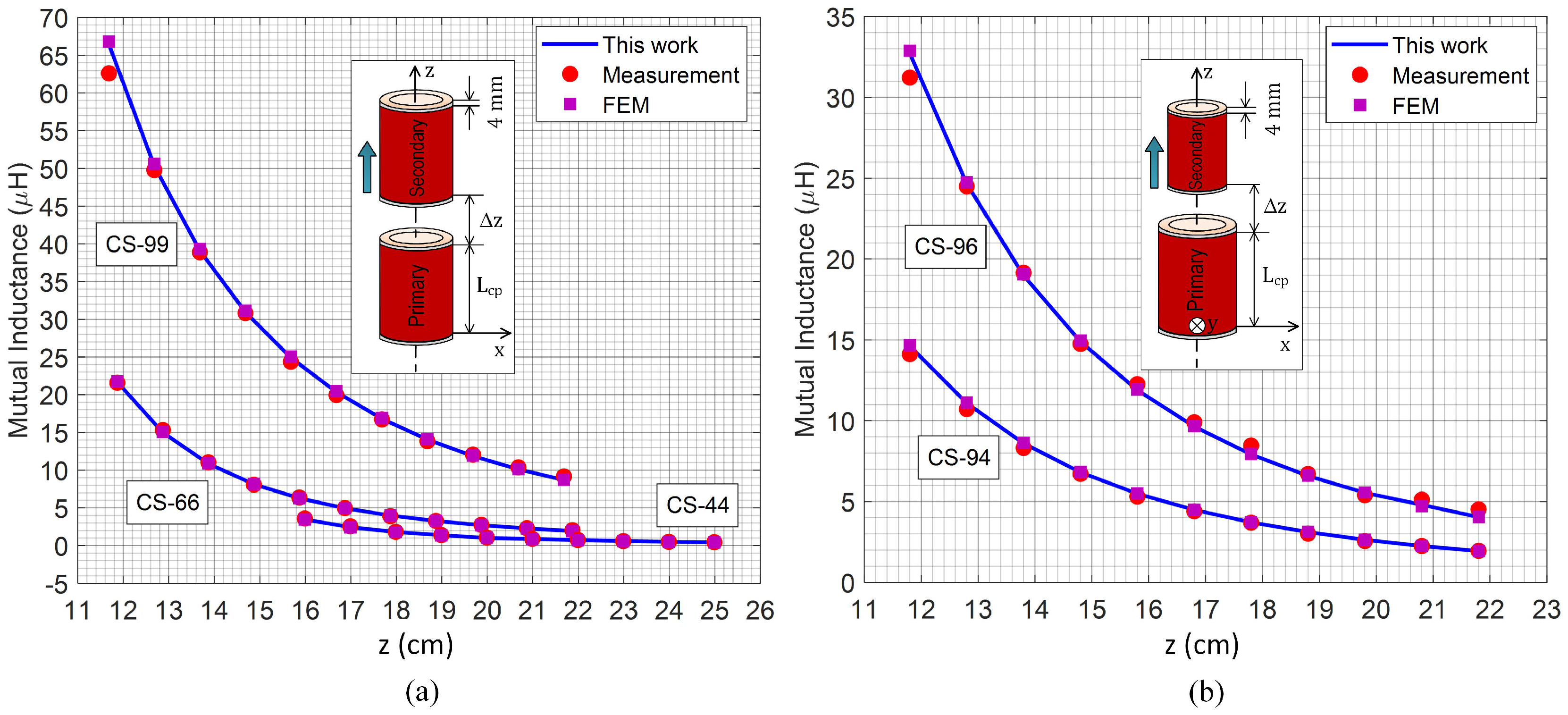
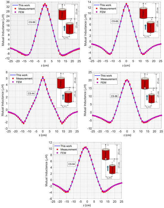
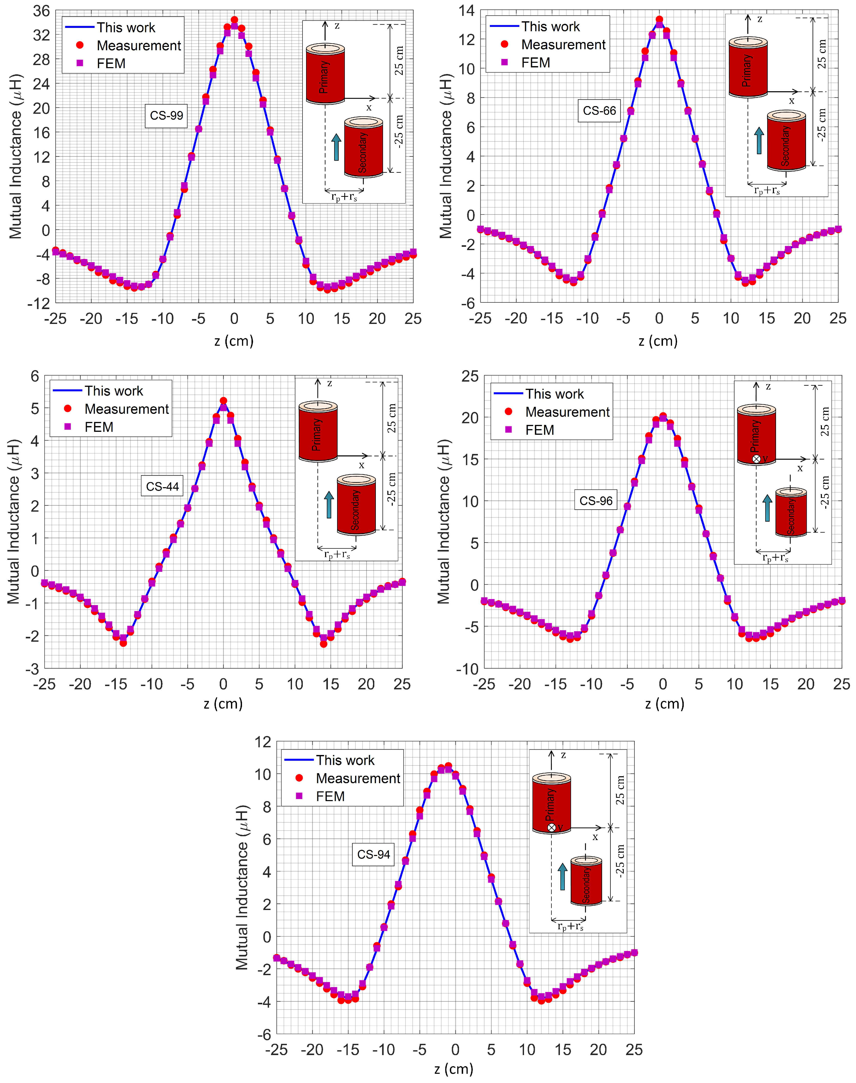
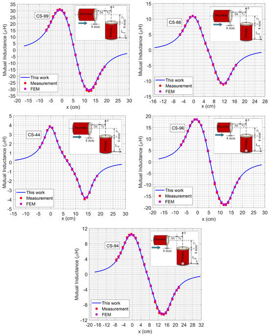
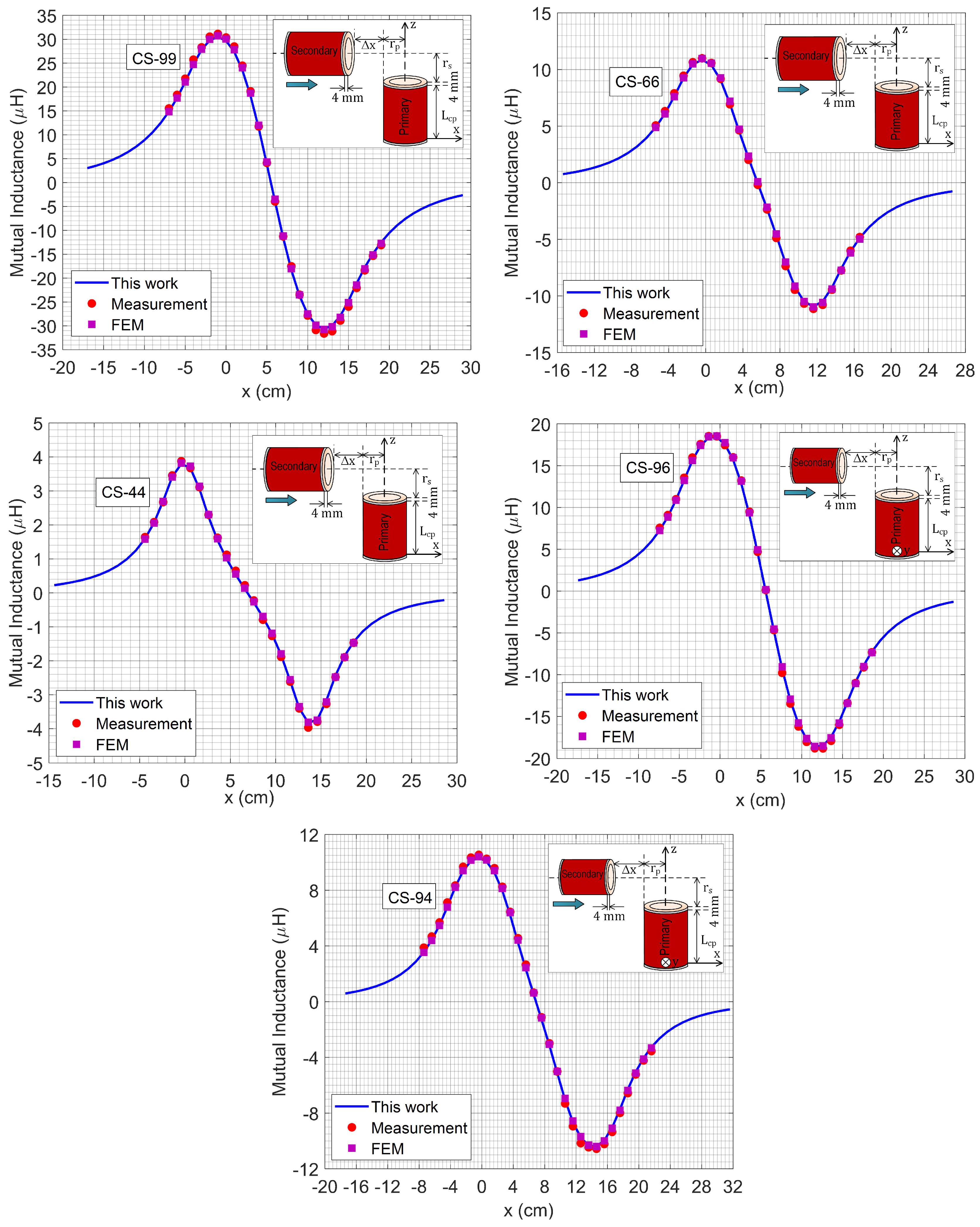
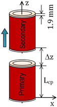
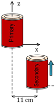
The SDC-A experimental configuration in Figure 8 was used to obtain experimental results for the coil positions in Figure 3a,d; the SDC-B configuration for the coil positions in Figure 3b,e; and the SDC-C and SDC-D configurations for the coil positions in Figure 3c,f. In the SDC-A configuration, with the primary coil held stationary, the secondary coil was incrementally displaced along the z-axis, and the resulting MI variation graphics, obtained analytically, via FEM, and through experimental measurements, are depicted in Figure 9. The MI variation graphics for the CS-99, CS-66, and CS-44 coil systems in Figure 9a are coaxial due to equal primary and secondary coil diameters, whereas those for the CS-96 and CS-94 systems in Figure 9b are non-coaxial due to unequal diameters, with the coil axes remaining parallel and displaced by $r_p-r_s$ along the y-axis. As expected, in all coil systems according to the SDC-A configuration, the MI variation graphics decreased similarly in a hyperbolic manner as the secondary coil moved further away from the primary coil in the z-axis direction. Furthermore, it can be observed that the FEM and experimental results are consistent with the analytical results of the MI calculation model. Similarly, for all coil systems listed in Table 2, under the SDC-B configuration, the primary coil was held stationary while the secondary coil was displaced along the x-axis by a distance of $r_p+r_s$, and then translated along the z-axis in 1 cm increments from −25 cm to +25 cm. The experimental MI results, together with the corresponding FEM and analytical results, are presented in Figure 10. As shown in this figure, the maximum magnetic coupling occurs in coil systems where the primary and secondary coil lengths are approximately equal (CS-99, CS-66, CS-44, CS-96), corresponding to the position where the coil bases are aligned. In the CS-94 coil system, since the secondary coil is longer than primary coil, the point of maximum coupling shifts to a different position compared to the other systems. When the primary coil is fixed and the secondary coil is displaced along the $\pm z$-axis beyond certain positions, the magnetic coupling reverses its direction. As a result, two negative peak values are obtained, one located in the $+z$ direction and the other in the $-z$ direction. This effect is clearly observed in the MI variation curves of all coil configurations presented in Figure 10. Moreover, it can be observed that the MI variation provided for CS-99 coil system corresponds to a portion of the 3D plot shown in Figure 7a.

Figure 9. Comparison of MI variation versus z-displacement of the secondary coil for the systems: (a) CS-99, CS-66, CS-44 and (b) CS-96, CS-94.

Figure 10. MI variation versus z-displacement of the secondary coil after lateral shift along the x-axis for the coil systems CS-99, CS-66, CS-44, CS-96 and CS-94.

In the MI variation graphics presented in Figure 11, based on the SDC-C configuration, the primary coil is kept fixed while the secondary coil is first rotated by $90°$ about the y-axis and then displaced along the z-axis by a distance equal to the sum of the length of the primary coil and the radius of the secondary coil. Subsequently, it is moved along the x-axis in 1 cm increments, and for each step position, experimental, FEM, and analytical results are obtained for all coil systems. As shown in the figure, when the secondary coil is displaced along the x-axis, the MI variation graph reaches peak values at a certain position when the coil is on the left side of the primary coil and at another position when it is on the right side. Additionally, it is observed that the MI value approaches zero when the secondary coil moves far away from the primary coil on either side. Besides, the MI variation for the CS-99 coil system appears as a section of the 3D plot depicted in Figure 7b.

Figure 11. MI variation versus x-displacement of the secondary coil after angular rotation about y-axis for the coil systems CS-99, CS-66, CS-44, CS-96 and CS-94.

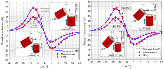
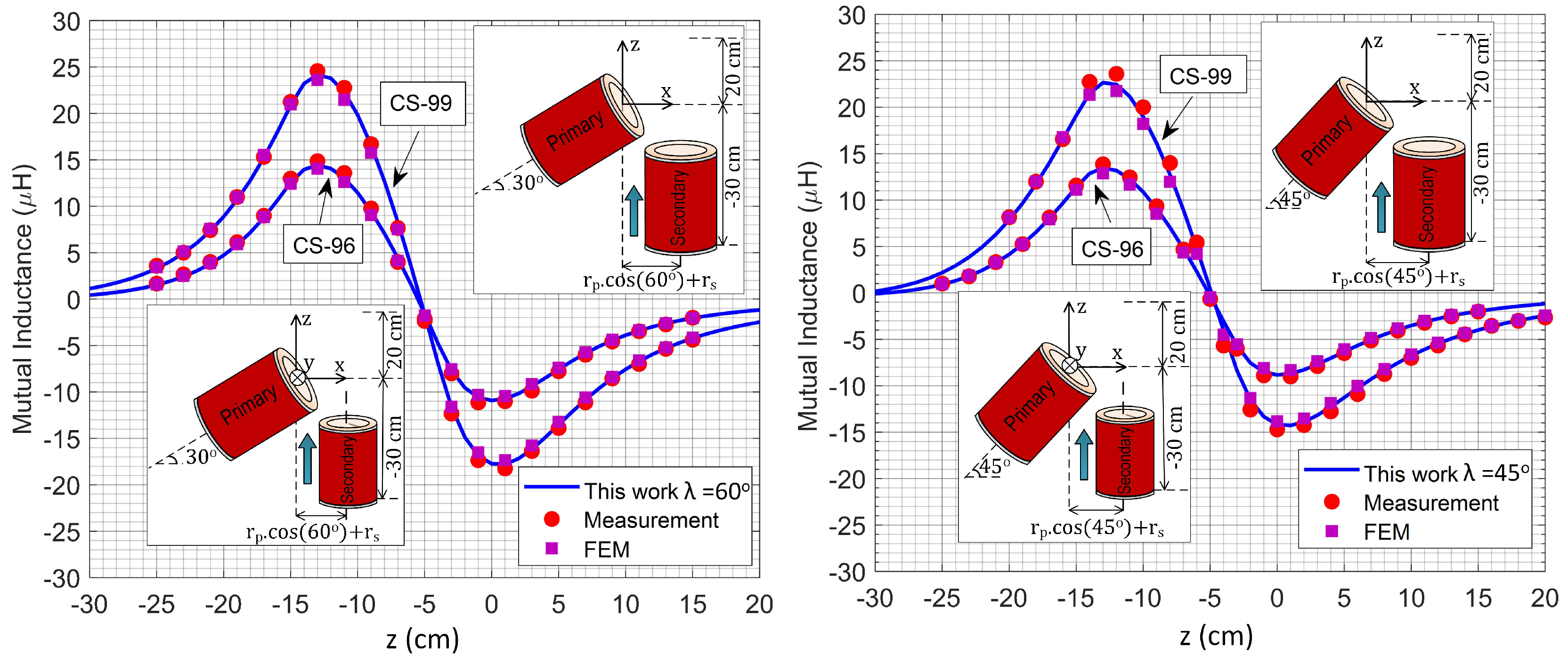
The MI variation plots shown in Figure 12 were obtained based on the SDC-D configuration. The primary coil was rotated about the y-axis, while the secondary coil was translated along the x-axis by a distance of $r_p\cos \left(\lambda \right)+r_s$. Subsequently, the secondary coil was moved along the z-axis from −30 cm to 20 cm in 1 cm increments. For each position, the MI was experimentally measured, and the corresponding values were calculated using the FEM and the proposed analytical model. The results presented in In Figure 12, the angle between the primary and secondary coil axes was considered at two different values, $\lambda$ = $60°$ and $\lambda$ = $45°$ for both the CS-99 and CS-96 coil systems. For the CS-99 coil system, the graphical results corresponding to $\lambda$ = $45°$ form part of the 3D plot group shown in Figure 7c. The plots also indicate that the calculated MI becomes negative in some configurations. This sign reversal occurs when the net magnetic flux linking the secondary coil is oriented opposite to the selected positive surface normal of the secondary coil.

Figure 12. MI variation versus z-displacement of the secondary coil after lateral shift along the x-axis and angular rotation of the primary coil about the y-axis for the coil systems CS-99 and CS-96.

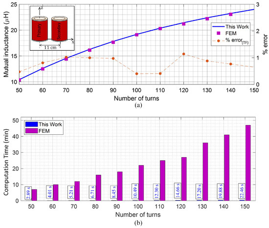
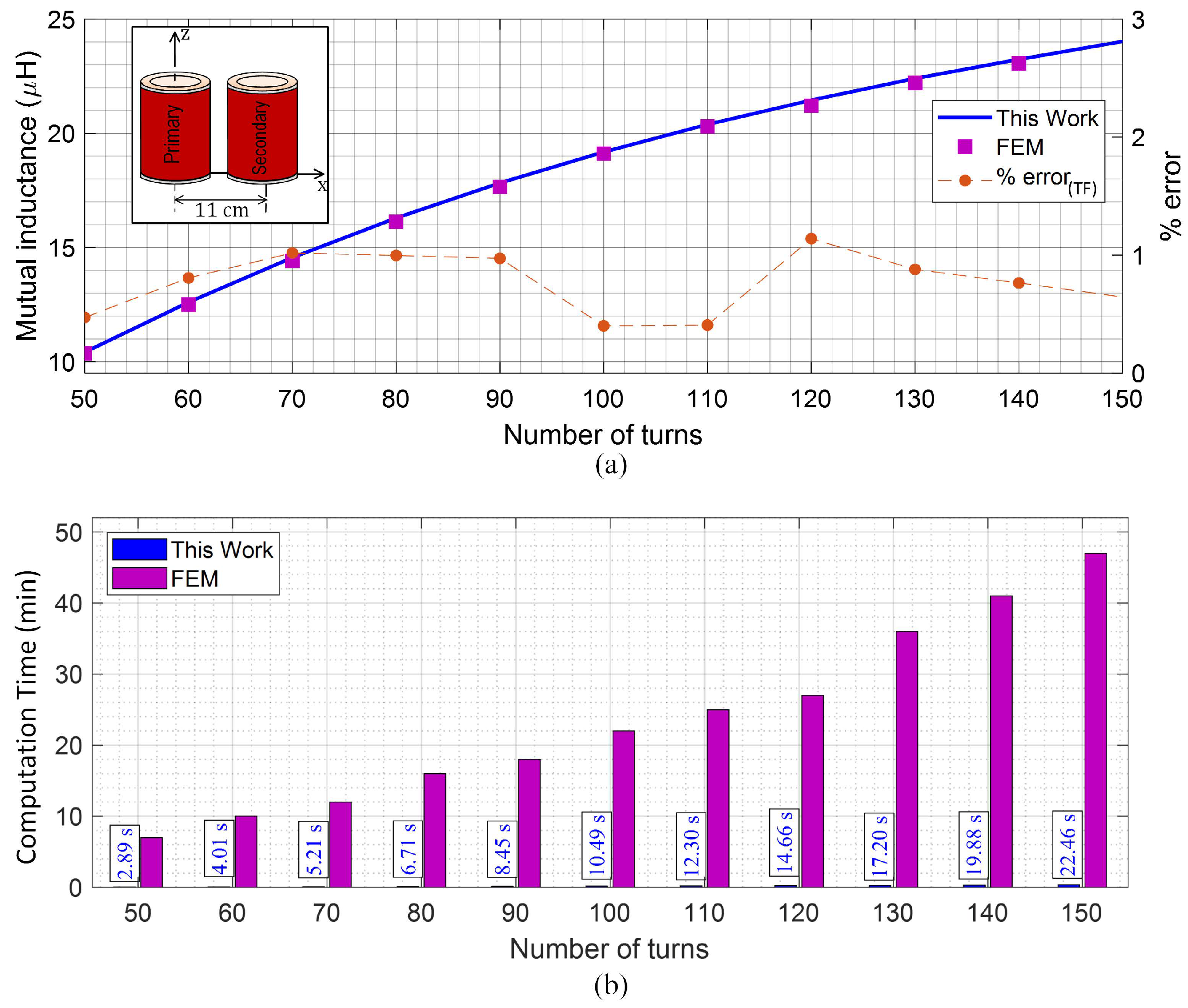
To evaluate the computational performance of the proposed formulation, a runtime analysis was performed for solenoid coil pairs with different numbers of turns. Two identical solenoid coils were arranged in the SDC-B configuration, where the coils were placed side by side with parallel axes and a center-to-center distance of 11 cm. Each coil had a radius of 5 cm, a wire diameter of 1 mm, and a spacing of 0.8 mm between consecutive turns. The primary and secondary coils were assigned the same number of turns in each case, and the turn number was varied from 50 to 150 in steps of 10. For each case, the MI values and computation times calculated using the proposed analytical model were compared with the corresponding FEM results and FEM computation times. The MI values, relative errors, and computation times for different turn numbers are presented in Figure 13. In Figure 13b, the bar heights are given in minutes for both methods, while the computation times of the proposed analytical model are additionally indicated in seconds above the corresponding bars for readability. The results show that the proposed analytical model maintains good agreement with the FEM results over the entire turn-number range. In addition, the analytical model requires considerably less computation time than the FEM analysis, demonstrating its computational advantage, particularly for high-turn coils and repeated parametric analyses.

Figure 13. Comparison of the proposed analytical model and FEM for solenoid coil pairs with different numbers of turns: (a) MI results and relative error, and (b) computation time.

Table 6 presents the MI results obtained from this work, FEM, and experimental measurements for different spatial displacement configurations of the CS-1010 coil system. The table also includes the corresponding relative errors between the proposed analytical model and the FEM and experimental results. As can be seen from the table, the results obtained from this work are in good agreement with the FEM results for the investigated displacement cases, confirming the accuracy of the proposed model under different spatial positioning conditions. The relative errors between the results of this work and the results of FEM and measurement were calculated ${\epsilon }_{TF}=100·|M_T-M_F|/M_T$ and ${\epsilon }_{TM}=100·|M_T-M_M|/M_T$, respectively.

Table 6. Comparison of this work, FEM, and experimental MI results under different spatial displacement configurations for CS-1010.

Spatial Displacement Configuration	Distance (cm)	Mutual Inductance (µH)			Error (%)
		This Work	FEM	Measurement	${ϵ}_{\mathit{TF}}$	${ϵ}_{\mathit{TM}}$
SDC-A	$z=13.8$	30.4195	30.1468	30.315	0.89	0.34
	$z=14.8$	23.8450	23.6179	24.125	0.95	1.17
	$z=15.8$	19.0428	18.8521	19.255	1.00	1.11
	$z=16.8$	15.4395	15.2775	15.856	1.05	2.69
	$z=17.8$	12.6826	12.5424	12.997	1.11	2.48
	$z=18.8$	10.5393	10.4164	10.839	1.17	2.84
SDC-B	$z=-3$	9.6701	9.4757	9.955	2.01	2.94
	$z=-2$	11.1497	10.9565	11.345	1.73	1.75
	$z=-1$	12.3504	12.1669	12.625	1.48	2.22
	$z=4$	10.8724	10.9686	11.175	0.88	2.78
	$z=5$	9.3509	9.5089	9.575	1.69	2.39
	$z=6$	7.6786	7.7875	7.925	1.42	3.21
SDC-C	$x=-6$	10.4275	10.3020	10.095	1.20	3.18
	$x=-5$	12.2514	12.1190	11.925	1.08	2.66
	$x=-4$	14.0277	13.9261	13.725	0.72	2.15
	$x=1$	14.1946	14.1123	13.978	0.58	1.52
	$x=2$	12.0825	12.1823	11.782	0.83	2.48
	$x=3$	9.2055	9.2534	8.967	0.52	2.59

Experimental measurements and FEM results showed good agreement with the analytically calculated values. This agreement demonstrates the accuracy and reliability of the developed analytical model. The MI calculation model’s capability to accurately compute MI under varying geometric configurations provides valuable insights for optimizing coil arrangements in a wide range of applications, including wireless power transfer, inductive sensing, and electromagnetic system design.

5. Conclusions

In this work, an analytical approach is presented for calculating the MI of coil systems composed of circular-wound solenoid coils using the MVP. A real solenoid coil, which has a helical structure, is modeled as if it consists of circular-wound filaments stacked along the axial direction. Each circular filament is considered equivalent to a polygonal filament with a sufficiently large number of sides, thereby forming a 3D model of the solenoid coils.

The proposed calculation model enables the determination of MI values for coil systems composed of solenoid coils with identical or different geometric parameters, considering all possible lateral and angular misalignments between the coils using a single analytical formula. This approach allows for MI calculations between solenoid coils to be performed with high accuracy and reduced computational load. Furthermore, the study presents various graphical results corresponding to misalignment conditions that have not been previously used in the literature. The results obtained from the proposed analytical formulas are compared with both experimental measurements and values obtained using the FEM. The observed high level of agreement among all results validates the accuracy and reliability of the developed analytical approach.

In this context, the developed model can be considered an effective tool for the design and optimization of electromagnetic systems involving solenoid coils. The proposed approach provides designers with an analytical and rapid evaluation capability for determining coil geometries, optimizing relative positioning between coils, and predicting the effects of misalignment on system performance. Accordingly, the model can be used as a reliable and efficient computational tool in applications involving solenoid coils for preliminary design and performance enhancement studies.

References

- Ma, L.; Zhang, H.; Zheng, W.; Shi, H.; Wang, C.; Xie, Y. Investigation on the Effect of Debris Position on the Sensitivity of the Inductive Debris Sensor. IEEE Sens. J. 2023, 23, 4438–4444. [Google Scholar] [CrossRef] [Scilit]
- Chladny, R.R.; Koch, C.R.; Lynch, A.F. Modeling automotive gas-exchange solenoid valve actuators. IEEE Trans. Magn. 2005, 41, 1155–1162. [Google Scholar] [CrossRef] [Scilit]
- Fujita, T.; Yasuda, T.; Akagi, H. A Dynamic Wireless Power Transfer System Applicable to a Stationary System. IEEE Trans. Ind. Appl. 2017, 53, 3748–3757. [Google Scholar] [CrossRef] [Scilit]
- Wang, D.; Li, W.; Zheng, J.; Cui, X.; Peng, S.; Zhou, D.; Guo, Y.; Cai, C. Influence of Coil Structure and Operating Frequency on Performance of Superconducting Wireless Power Transfer. IEEE Trans. Appl. Supercond. 2025, 35, 4606509. [Google Scholar] [CrossRef] [Scilit]
- Deng, Q.; Liu, J.; Czarkowski, D.; Kazimierczuk, M.K.; Bojarski, M.; Zhou, H.; Hu, W. Frequency-Dependent Resistance of Litz-Wire Square Solenoid Coils and Quality Factor Optimization for Wireless Power Transfer. IEEE Trans. Ind. Electron. 2016, 63, 2825–2837. [Google Scholar] [CrossRef]
- Gordan, U.; Jayalath, S. Comparative Analysis of Wireless Power Transfer Couplers for Unmanned Aerial Vehicles and Drones. IEEE Open J. Power Electron. 2024, 5, 618–633. [Google Scholar] [CrossRef] [Scilit]
- Feng, T.; Shi, K.; Jiang, J.; Wang, P. A Solenoid Magnetic Coupler and Its Control Method for Omnidirectional Wireless Charging of UAVs. IEEE Trans. Ind. Electron. 2025, 72, 2540–2550. [Google Scholar] [CrossRef] [Scilit]
- Zhu, J.; Li, Y.; Jin, C.; Liu, X.; Liu, H. Optimum Separation for Performance Improvement of RFID Solenoid Coil Antenna in Metallic Environments. IEEE Antennas Wirel. Propag. Lett. 2021, 20, 1611–1615. [Google Scholar] [CrossRef] [Scilit]
- Kolagar, A.D.; Rashidzadeh, J.; Arjanaki, A.A.; Pahlavani, M.R.A. Design, Simulation, and Implementation of Stranded Solenoid Coil With Variable Inductance for Use in Loran Transmitter. IEEE Trans. Plasma Sci. 2020, 48, 2544–2553. [Google Scholar] [CrossRef] [Scilit]
- Peng, S.; Sheng, J.; Yang, Z.; Zhou, X.; Wang, X.; Zhao, R.; Zhang, X.; Yang, K.; Jin, Z. Electromagnetic Analysis of Solenoid Coil Wound With Multilayer CORC Cable. IEEE Trans. Appl. Supercond. 2026, 36, 4601406. [Google Scholar] [CrossRef] [Scilit]
- Horiuchi, Y.; Yamasaki, Y.; Ezaki, T.; Imayoshi, T. Solenoid Type Shielding Coil Systems for a Small Scale SMES. IEEE Trans. Appl. Supercond. 2008, 18, 709–712. [Google Scholar] [CrossRef] [Scilit]
- Huang, L.; Murray, A.; Flynn, B.W. Optimal Design of a 3-Coil Wireless Power Transfer System for Deep Micro-Implants. IEEE Access 2020, 8, 193183–193201. [Google Scholar] [CrossRef] [Scilit]
- Cheng, Y.; Wang, G.; Ghovanloo, M. Analytical Modeling and Optimization of Small Solenoid Coils for Millimeter-Sized Biomedical Implants. IEEE Trans. Microw. Theory Techn. 2017, 65, 1024–1035. [Google Scholar] [CrossRef] [Scilit]
- Congo, M.G.; Perdriau, R.; Stojanovic, M.; Koohestani, M.; Lafon, F.; Ramdani, M. Analytical Model for Mutual Inductance Prediction Between Horizontal Inductors With Arbitrary Orientations. IEEE Lett. Electromagn. Compat. Pract. Appl. 2026, 8, 11–16. [Google Scholar] [CrossRef] [Scilit]
- Kovačević, I.F.; Friedli, T.; Müsing, A.M.; Kolar, J.W. 3-D Electromagnetic Modeling of Parasitics and Mutual Coupling in EMI Filters. IEEE Trans. Power Electron. 2014, 29, 135–149. [Google Scholar] [CrossRef] [Scilit]
- Maxwell, J.C. A Treatise on Electricity and Magnetism; Clarendon Press: Oxford, UK, 1873. [Google Scholar]
- Rosa, E.B.; Cohen, L. The mutual inductance of coaxial solenoids. Bull. Bur. Stand. 1907, 3, 305–324. [Google Scholar] [CrossRef] [Scilit]
- Rosa, E.B.; Grover, F.W. Formulas and Tables for the Calculation of Mutual and Self-Inductance; Scientific Papers of the Bureau of Standards. No. 169; Washington, Government Printing Office: Washington, DC, USA, 1916. [CrossRef] [Scilit]
- Dwight, H.B.; Grover, F.W. Some series formulas for mutual inductance of solenoids. Electr. Eng. 1937, 56, 347–353. [Google Scholar] [CrossRef] [Scilit]
- Grover, F.W. Tables for the calculation of the mutual inductance of any two coaxial single-layer coils. Proc. Inst. Radio Eng. 1933, 21, 1039–1049. [Google Scholar] [CrossRef] [Scilit]
- Conway, J.T. Inductance Calculations for Noncoaxial Coils Using Bessel Functions. IEEE Trans. Magn. 2007, 43, 1023–1034. [Google Scholar] [CrossRef] [Scilit]
- Conway, J.T. Exact solutions for the mutual inductance of circular coils and elliptic coils. IEEE Trans. Magn. 2012, 48, 81–94. [Google Scholar] [CrossRef] [Scilit]
- Conway, J.T. Mutual inductance of thick coils for arbitrary relative orientation and position. In Progress in Electromagnetics Research Symposium-Fall (PIERS-FALL); IEEE: Singapore, 2017. [Google Scholar] [CrossRef] [Scilit]
- Hurley, W.G.; Duffy, M.C.; Zhang, J.; Lope, I.; Kunz, B.; Wölfle, W.H. A Unified Approach to the Calculation of Self- and Mutual-Inductance for Coaxial Coils in Air. IEEE Trans. Power Electron. 2015, 30, 6155–6162. [Google Scholar] [CrossRef] [Scilit]
- Babic, S.; Akyel, C. Improvement in calculation of the self- and mutual inductance of thin-wall solenoids and disk coils. IEEE TRans. Magn. 2000, 36, 1970–1975. [Google Scholar] [CrossRef] [Scilit]
- Babic, S.; Mastorakis, N.E. A novel semi-analytical regular and singular solutions for calculating mutual inductance between inclined solenoids in crossing or contact positions. WSEAS Trans. Syst. 2025, 24, 44–51. [Google Scholar] [CrossRef] [Scilit]
- Pankrac, V. Generalization of Relations for Calculating the Mutual Inductance of Coaxial Coils in Terms of Their Applicability to Non-Coaxial Coils. IEEE Trans. Magn. 2011, 47, 4552–4563. [Google Scholar] [CrossRef] [Scilit]
- Altun, H.; Pirinççi, N. A Novel Analytical Model for Mutual Inductance Calculations Between Two Nonidentical N-Sided Polygonal Planar Coils Arbitrarily Positioned in 3-D Space for Wireless Power Transfer. IEEE Trans. Power Electron. 2023, 38, 10396–10411. [Google Scholar] [CrossRef] [Scilit]
- Pirinççi, N.; Altun, H. A New Analytical Study on Mutual Inductance Calculations for Wireless Power Transfer Using Magnetic Vector Potential. IEEE Trans. Magn. 2022, 58, 8002714. [Google Scholar] [CrossRef] [Scilit]
- Haus, H.A.; Melcher, J.R. Electromagnetic Fields and Energy; Prentice-Hall: Englewood Cliffs, NJ, USA, 1989. [Google Scholar]
Disclaimer/Publisher’s Note: The statements, opinions and data contained in all publications are solely those of the individual author(s) and contributor(s) and not of MDPI and/or the editor(s). MDPI and/or the editor(s) disclaim responsibility for any injury to people or property resulting from any ideas, methods, instructions or products referred to in the content. |
© 2026 by the authors. Licensee MDPI, Basel, Switzerland. This article is an open access article distributed under the terms and conditions of the Creative Commons Attribution (CC BY) license.