


Abstract
Urban air pollution, especially the problem of PM2.5, is one of the major health challenges facing the planet today. To provide accurate PM2.5 predictions despite data noise and missing data, the authors proposed a deep learning model. We constructed a Stacked Autoencoder–Convolutional Neural Network–Bidirectional Long Short-Term Memory–Long Short-Term Memory (SAE-CNN-BiLSTM-LSTM) model that (1) utilises convolutional layers to extract spatial features from the input data, (2) employs bidirectional LSTM layers to capture long-term temporal dependencies, and (3) utilises an autoencoder to learn latent representations of the data to mitigate the effects of missing data. The model was trained on a large dataset of hourly measurements of air quality and meteorological parameters collected between 2018 and 2020 in Klang, Malaysia. The performance of the model on data that were not used during training was evaluated using a range of metrics. The SAE-CNN-BiLSTM-LSTM model achieved a test RMSE of approximately 11.97 µg/m3 and an R2 statistic of approximately 0.85 for PM2.5 concentrations, outperforming the other models tested on the same datasets. The additional metrics of MAE, MAPE, Mean Bias Error, and Index of Agreement confirmed the model’s accuracy and low bias in the prediction of air pollution levels. Statistical tests, such as the Diebold–Mariano test, confirmed the significance of the model’s accuracy over the CNN-LSTM models. These findings indicate that the proposed model effectively captures the dynamics of the air pollution data. The proposed model structure efficiently achieved an accurate and lightweight model for urban air pollution forecasting.
1. Introduction
In recent years, the economies of most countries have developed rapidly, and the problem of air pollution has attracted the attention of most people worldwide [1]. Air pollution incidents caused by fine particulate matter (PM2.5) have occurred frequently and have become the main environmental problem in most cities and regions of the country [2]. PM2.5 consists of particles with small radii containing various toxic and harmful substances, such as heavy metals. These particles remain suspended in the air and pose a significant threat to the lives and health of people [3]. The ability to accurately and reliably predict air pollution incidents would provide warnings and decision-making support to the public and governmental agencies in the case of these serious environmental incidents [4]. Thus, it is urgent to accurately and reliably predict the concentration of PM2.5 in the environment to control air pollution and protect the health of the people, which is of great practical significance [5].
At present, there are three main models for predicting air pollutant concentrations: numerical, statistical, and machine learning-based prediction models [6,7]. Numerical models simulate the physical and chemical changes and transport processes of pollutants in the atmosphere by constructing and solving complex differential equations [8]. Representative numerical models include the Common Multiscale Air Quality Model (CMAQ) and Weather Research and Forecasting Model (WRF-Chem) [9]. However, the accuracy of these models is highly dependent on detailed pollutant source emission data, leading to uncertainty in the actual predictions [10].
The second model is based on data-driven mining of internal relationships in the historical data. Common statistical models include classical statistical models such as ARIMA and ARMA [11]. Because statistical models do not involve complex physical changes, chemical reactions, or transport processes, their computational cost of statistical models is lower than that of numerical models. However, such models are mainly suitable for small datasets and univariate time series modelling and have strict requirements for the stationarity of data, which greatly limits the performance and applicability of classical statistical models in air pollution prediction.
In the last few years, there has been a focus on developing prediction models based on machine learning, such as random forest (RF) and artificial neural networks (ANNs) [12]. However, these models often require researchers to manually construct features, which heavily relies on their personal experience. Additionally, when dealing with large datasets, they show insufficient ability to reduce redundant data, which in turn affects their learning and generalisation capabilities. Therefore, it is necessary to build more accurate models to improve air pollution prediction. As the latest achievement in machine learning, deep learning algorithms have excellent self-learning and nonlinear mapping abilities, making them widely applicable in the field of air pollution prediction [13]. Among them, recurrent neural networks (RNNs) and their variants [14], such as long short-term memory (LSTM) [15] and gated recurrent units (GRUs), are specifically used for sequence prediction.
However, air pollution prediction requires modelling the spatiotemporal relationship between various complex and non-stationary air pollutant data and meteorological data, and a single RNN-based model may be insufficient to handle spatiotemporal dependent datasets. To address the limitations of a single deep learning model, hybrid models have been developed, such as the CNN-LSTM [16] algorithm, GCN, and GRU [17], to enhance spatiotemporal modelling. Despite the significant progress in deep-learning-based air pollution forecasting, several limitations remain unresolved. Most existing studies focus on urban environments with relatively stable emission patterns or rely on extensive multi-source data such as emission inventories and satellite observations. However, industrial coastal cities, where pollution dynamics are influenced by complex interactions between maritime activities, industrial emissions, and meteorological variability, have received limited attention in the literature. Moreover, although deep learning models demonstrate high accuracy in making predictions, they fail to exhibit robustness in the presence of incomplete and noisy data. Hence, there is a need for a compact yet effective deep learning model capable of learning the nonlinear patterns in the data. In this study, a deep learning model based on stacked autoencoders combined with CNNs, BiLSTMs, and LSTMs was proposed for a one-step air quality prediction task in Klang, Malaysia [18].
To investigate the spatiotemporal characteristics of the evolution of PM2.5 concentrations in Malaysia, this study utilised a stacked autoencoder model to predict the PM2.5 concentrations and conducted horizontal comparisons to explore the spatiotemporal characteristics of the PM2.5 data. The main contributions of this study are as follows.
- Technical Novelty: The incorporation of a deep autoencoder with a hybrid CNN-BiLSTM-LSTM model presents a new method for predicting PM2.5 and PM10 concentrations. Unlike other methods using stacked autoencoders, the use of convolutional and BiLSTM-LSTM layers allows for the model to extract features from the data while understanding the complicated temporal relationships within the data regarding PM2.5 and PM10 concentrations. This study also used a hybrid training process that improved the accuracy of the predictions by optimising both the reconstruction (autoencoder) and forecasting goals. This makes predictions more accurate even when data are lacking or noisy
- Contextual Novelty: This study used our proposed model on a large dataset of air quality data from Klang, Malaysia. Data were collected from 1 January 2018 to 31 December 2020. Given the lack of previous research on this specific dataset and geographical location with these types of deep learning methods, our work will provide new information regarding the change in pollution in these types of cities.
- Comprehensive Benchmarking: While other studies compare the proposed models to classical machine learning models, we tested the proposed architecture against state-of-the-art deep learning models. These include models based on long short-term memory (LSTM) networks, convolutional LSTM (CNN-LSTM) models, and more recent transformer models that employ recurrent neural networks. Thus, our study provides a more thorough and comprehensive evaluation of the usefulness and performance of the proposed method than previous studies.
2. Related Works
2.1. Classical and Shallow Learning for PM Forecasting
Owing to their simplicity, classical statistical methods have been used for forecasting tasks. Two of the most common methods are the ARIMA and ETS models. For example, Jeon and Han [19] used monthly PM2.5 data from Seoul over a 4-year period (2015–2018) to train and test the performance of an ARIMA and an ETS model in forecasting the PM2.5 concentration 12 months ahead. Given that the ETS outperformed the ARIMA model (RMSE = 5.84 µg/m3 vs. 7.73 µg/m3), the researchers also noted that the linear structure of the ARIMA model makes it less suitable for air quality data that include these complex undertones. Shallow machine learning models have also been applied to this problem, including models as seemingly simple as Support Vector Regression (SVR), Random Forest (RF), and Gradient Boosting Machines (GBMs). Kim et al. [20] used tree-based models (LGB, RF, XGB) for 36 h PM2.5 prediction in Seoul, achieving RMSE = 7.48 µg/m3 (R2 = 0.83) for PM2.5. Hence, traditional and shallow ML models can improve linear models by capturing nonlinear relationships but do not account for all the complexities of spatiotemporal data. Although these models exhibit strong reliability and interpretability, they lack the necessary capacity to handle nonlinear dynamics in urban air pollution data.
2.2. Deep Learning for Air Pollution Prediction
In the last few years, deep learning has become the standard for PM2.5/PM10 forecasting methods due to its ability to learn complex spatial–temporal patterns [21], and the Deep-AIR model was proposed, which is a CNN–LSTM hybrid forecasting model applied to Hong Kong and Beijing. It achieved up to 77% accuracy for 1 h forecasts and ~65% for 24 h forecasts, demonstrating strong performance in spatiotemporal prediction tasks. Likewise, Bai et al. [22] developed a CNN–LSTM model for daily PM2.5 forecasting in Qingdao, China. Training on data from 2020, they achieved R2 = 0.91 and RMSE = 8.22 µg/m3, outperforming standalone CNN (R2 = 0.85) and LSTM (R2 = 0.83). Their model combined CNN for spatial feature extraction and LSTM for temporal sequence modelling. These studies demonstrate that CNN–LSTM hybrids are effective in capturing local spatio-temporal connections; however, they face difficulties with long-range inter-station interdependence and exhibit a lack of robustness in situations characterised by significant noise or missing data. Other studies have focused on attention-based and transformer architectures. Hence, transformer-based models with attention mechanisms have enhanced long-term dependency modelling in air quality forecasting. Li et al. [23], introduced a CBAM–CNN–BiLSTM model across Beijing stations, associating spatial attention with bidirectional LSTM to enhance 1–48 h PM2.5 forecasts; the model maintained strong accuracy for up to 48 h (R2 ≈ 0.94, RMSE ≈ 18.9 µg/m3). Although related transformer-specific variants were beyond our accessible sources, we recognise that such attention-based models typically achieve higher accuracy but increase computational complexity, posing challenges for real-time deployment.
Although federated learning techniques have not yet been deeply explored in mainstream air pollution modelling, they promise privacy-preserving distributed data training. Hu et al. [24] introduced FedDeep: A Federated Deep Learning Network for Edge-Assisted Multi-Urban PM2.5 Forecasting, implemented across municipal regions in China (e.g., Jiangsu Province). Their system uses an external spatiotemporal network (ESTNet) deployed on edge cloud servers, enabling localised training with meteorological and pollution data. Model updates were aggregated in a central server, achieving MAE = 12.38, RMSE = 19.19, and R2 = 0.972 for 12 h PM2.5 forecasts, while requiring just ~0.87 GB GPU memory and ~28 min training time. However, its reliance on network connectivity and consistent local data quality highlights the challenges of real-world deployment. Thus, in this study, we propose a stacked deep autoencoder model that incorporates CNN and BiLSTM–LSTM layers within an autoencoder framework. This design has the following features:
- Learns hierarchical spatial–temporal features directly from data, eliminating manual feature crafting.
- Handles missing or noisy data via reconstruction losses in the autoencoder, improving robustness.
- Captures long-term dependencies through stacked BiLSTM/LSTM units.
- Balances performance and efficiency, requiring less computational overhead than full attention/transformer models.
- Adapts well to real-time systems, due to its simplified structure compared to more complex models.
In combination, these characteristics enable superior PM2.5 forecasting performance with greater practicality for the deployment. Unlike federated models, our architecture is optimised for centralised applications with complete control over data preprocessing and modelling; however, future extensions could integrate federated training. Table 1 summarises the research gap identification for this study.
Table 1.
Research gap identification.
3. Study Area and Dataset Analysis
3.1. Geographic and Environmental Context
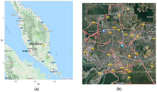
Klang, Malaysia (latitude 3.03° N, longitude 101.45° E), is a coastal, industrialised city located in the state of Selangor and serves as home to Port Klang, one of the largest maritime ports in Southeast Asia. The rapid urbanisation, industrialisation, and traffic congestion that characterise Klang have led to high levels of air pollution. Klang is subject to two monsoon systems that reverse their direction throughout the year: the Southwest Monsoon, which occurs between May and September, and the Northeast Monsoon, which occurs between November and March. These monsoons have a major influence on the movement of air pollution within the city, particularly in relation to the levels of PM2.5 and PM10 pollution that exists within the city [25]. Figure 1a shows the location of Klang within Peninsular Malaysia, and Figure 1b depicts the layout of the city. Accurately modelling PM2.5 within the city of Klang is important for assessing the health risks to the city’s population, yet challenging owing to the spatial and temporal variability of PM2.5 pollution from both meteorological and anthropogenic sources within the city.
Figure 1.
(a) Map of Peninsular Malaysia with Klang marked with a red dot; (b) map of Klang.
3.2. Data Description and Preprocessing
- Data Description
The data utilised in this study were obtained from two governmental agencies in Malaysia:
- Department of Environment (DOE), Malaysia: Source of data regarding the air quality measurements taken hourly at various monitoring stations across the country.
- Malaysian Meteorological Department (METMalaysia) [17]: Source of meteorological data; available from 1 January 2018, until 31 December 2020. All data are made publicly available by the government and recorded every hour, yielding over 26,000 time steps in each station’s dataset [26].
The three cities that will be studied are as follows:
- Klang (industrial port zone, primary target region);
- Shah Alam (residential–industrial corridor);
- Kuala Lumpur (urban capital zone).
This multi-station configuration allows the model to capture regional pollution transport dynamics, improving generalisation to spatially correlated events such as transboundary haze or urban spillover.
- Air Quality Parameters
Each station provides data on the concentration of pollutants present hourly, and the types of pollutants include the following [27]:
- Particulate matter: PM2.5 (fine particles), PM10 (coarse particles).
- Gaseous pollutants: NO2, SO2, CO, and O3.
All of these gases are measured using BAMs, TEOM sensors, and gas analysers that are either in compliance with DOE [28] calibration protocols or equivalent to US EPA Class III standards.
- Meteorological Parameters
Meteorological features were collocated at each station and included the following:
- Temperature (°C) and Relative Humidity (%);
- Wind Speed (m/s) and Wind Direction (°);
- Atmospheric Pressure (hPa) and Rainfall (mm).
However, these factors are also critical for understanding pollutant dispersion and transformation processes.
- Spatial Metadata
Each station is geotagged, and its metadata include the following (Table 2):
Table 2.
Data Source and summarizes the characteristics of the air quality monitoring stations.
- Temporal Coverage
All times are in Malaysia Standard Time (MST, UTC+8). The data were sampled hourly, enabling lag analyses and forecasting.
In total, the dataset includes the following:
- Nine pollutant and meteorological features per station.
- Approximately 26,304 hourly records per station.
- Three years × three stations = robust input for deep sequence models.
This setup supports the development of multivariate, multi-source models that are resilient to seasonal cycles, spatial spillover, and atmospheric noise—requirements that are directly addressed by the hybrid deep learning architecture described in Section 4.
- Missing Data Handling
Many environmental time-series datasets contain missing entries owing to sensor calibration requirements, logger and transmission issues, or weather conditions (e.g., lightning or haze). These missing entries have the potential to negatively impact model performance, especially for models based upon sequences of data, such as LSTMs and BiLSTMs.
To address this, a multi-stage imputation framework was adopted that considers the granularity of the timestamps associated with each variable and the type of information that each variable represents. The framework considers the following steps.
- Step 1 Assess the missingness of each variable: The missingness of each variable was assessed across all stations and for each individual station. The results of this assessment revealed the following:
Each variable had less than 5% of its values missing across all stations over the three-year period.
The missing values for each variable tended to be either randomly or weather-dependent, with a small number of missing values for each variable that were clustered during the monsoon period.
The relatively small amount of missing data for each variable indicates that it is possible to utilise statistical imputation methods to impute the missing values for each variable, and that it is not necessary to remove those time windows from the data.
- Step 2 (Short-Gap Imputation (≤3 h)): For gaps in the data of three hours or less, a hybrid of forward fill and linear interpolation techniques were used:
Applying forward fill helps maintain the trend of the data points over time.
Applying linear interpolation helps to even out the data points over time, while maintaining the trend of the data.
Applying these techniques to each of the features within each station helps ensure that the data points from each station are evened out.
- Step 3 (Long-Gap Exclusion (>3 h)): For records with gaps exceeding three hours, the records were excluded from the model training and evaluation processes. This approach was adopted for the following reasons:
This avoids introducing bias by filling such large gaps in the data. This prevents the contamination of LSTM memory cells with data that do not accurately represent the records in those gaps. It also ensures that the model is trained and evaluated on a sufficiently large and clean dataset.
- Step 4 (Sequence Integrity Checks): Following imputation, the dataset was segmented into sequences of fixed length to be used in training the prediction model. The segments used contained all data points after cleaning the dataset.
- Feature Scaling and Normalisation
Given the importance of feature scaling in deep neural network training, it is essential to note that deep learning algorithms might be affected significantly if the feature values have a wide range of scales (for instance, the pollution level of PM2.5 can be measured in μg/m3, the temperature in °C, and the wind direction in degrees). Poor normalisation of these features can result in the network having difficulties converging upon the optimal weights for the model. To address this issue, min–max normalisation was applied to the continuous variables and cyclical encoding was used for the time and directional variables to ensure that the magnitude and temporal relationships of the variables were preserved.
- Min–Max Normalisation
Each continuous feature (e.g., PM2.5, Temperature, Humidity) is independently scaled to the range using:
where and denote the minimum and maximum values calculated from the training set only. This approach ensures that no data leakage occurs from the test sets into the training process. Min–max scaling is well-suited for models with ReLU or sigmoid activation functions. Each feature was normalised independently from one another.
- Cyclical Feature Encoding
Variables with inherent cyclical behaviour—such as hour of day, day of week, month of year, and wind direction—require transformation that respects their circular topology (e.g., hour 23 and 0 are adjacent).
For each cyclical variable , two new features were generated:
where is the period (e.g., 24 for hour of day, 360 for wind direction). This representation has the following features:
- Avoids artificial discontinuities (e.g., between 359° and 0°);
- Preserves angular distance;
- Allows the model to learn periodic relationships in air pollution patterns.
Applied variables include the following:
- Wind Direction (°) → ;
- Hour of Day → ;
- Month → .
This dual-component encoding has proven effective in capturing rush-hour peaks, weekend effects, and monsoon seasonality, which are central to PM2.5 fluctuations.
- Resulting Feature Space
After all transformations, the final input vector for each hourly time step consists of the following:
- Numerical variables (e.g., PM2.5, humidity): scaled to [0, 1].
- Cyclical time and directional encodings: 2 values per variable.
- Station-specific pollutant and weather inputs: from the three cities (Klang, Shah Alam, and Kuala Lumpur).
This normalised and standardised representation allows the model to identify both short- and long-term trends in the data.
3.3. Dataset Characteristics and Challenges
Air quality and meteorological datasets have several nontrivial properties that pose challenges in creating effective deep learning models for their prediction. Understanding those properties enables the development of appropriate preprocessing steps and deep learning model architectures.
- Nonstationary and Seasonal Drift
The dataset is strongly influenced by Malaysia’s bimodal monsoon climate, which induces substantial seasonal drift in pollutant levels. For example:
- PM2.5 levels peak during the Southwest Monsoon (June–September) due to dry conditions and transboundary haze.
- High humidity and rainfall during the Northeast Monsoon (November–March) reduce particulate matter through washout effects.
These seasonal changes cause shifts in mean, variance, and autocorrelation structure, violating stationarity assumptions common to traditional time-series models (e.g., ARIMA). Augmented Dickey–Fuller (ADF) tests on the raw PM2.5 series confirm significant nonstationarity (), suggesting the need for robust, sequence-aware models with temporal memory.
- Meteorologically Coupled Noise
Pollutant behaviour is tightly coupled with meteorological variables:
- Wind speed and direction influence dispersion and transport of pollutants.
- Rainfall produces abrupt drops in PM concentration due to wet deposition.
- Humidity and temperature modulate chemical transformation and atmospheric mixing.
Given the complex and nonlinear relationships between meteorological variables, deep learning models with branches that run in parallel and perform different functions (such as the use of CNNs and LSTMs) are better models for these meteorological phenomena than shallow learning models.
- Skewed Distributions and Extreme Events
The distributions of both PM2.5 and PM10 exhibited positive skewness, indicated by the long tail to the right that exists in these distributions (due to haze, biomass burning, and industrial upsets events). These outliers have the ability to affect the results as follows:
- Distort statistical measures of the population of PM2.5 and PM10 particles;
- Bias the model training towards these values;
- Implement loss functions or normalisation steps to account for these outliers.
To address this issue, the use of min–max scaling with quantile clipping and autoencoders will help compress the data into a latent representation that is robust to these outliers.
- Multi-Station Spatial Correlation
Even though the target variable is Klang station, the other stations in the vicinity (for example, Shah Alam and Kuala Lumpur) are spatially and meteorologically correlated with Klang. Pollution episodes (e.g., regional haze) often simultaneously impact several cities. Thus, by using data from multiple stations as the model’s input, the model can learn of these dependencies between the stations, which will enable it to generalise to new conditions for those stations.
- Temporal Patterns and Periodicity
Pollutant levels follow diurnal, weekly, and seasonal cycles:
- Rush-hour peaks (07:00–09:00, 17:00–20:00);
- Lower emissions on weekends;
- Seasonal haze and monsoon-driven clearing.
These periodic signals were preserved using sinusoidal encoding of time variables (hour, day, month), enabling the model to learn cyclical patterns without overfitting.
- Missing Data and Sensor Drift
Despite quality assurance by DOE and METMalaysia, the dataset includes the following:
- Short gaps due to temporary signal loss or maintenance;
- Longer outages during severe weather;
- Potential sensor drift over time.
The preprocessing strategy described in Section 3 helps to deal with short gaps in the data and removes sequences that are determined to be unreliable. Furthermore, the use of an autoencoder within the model helps filter the data to remove any spurious signals introduced during preprocessing. These steps presented challenges that motivated the architecture of the model, which is described in Section 4. The use of CNN encoders, BiLSTM models for time series data, and an autoencoder–decoder model in the architecture of the model help to ensure the following:
- Nonstationary, nonlinear input series;
- No missing data;
- Periodic dependencies;
- Multi-source spatial interactions.
4. Methodology
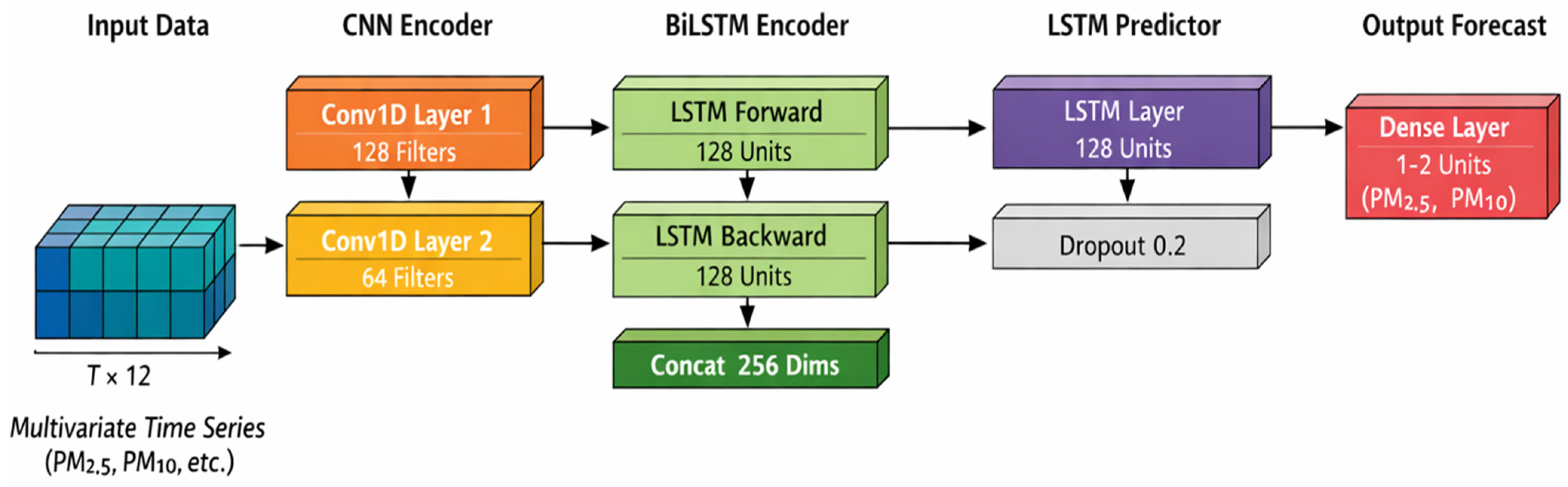
The proposed framework consists of three main modules: a convolutional neural network (CNN) to encode the spatial component of the problem, a bidirectional long short-term memory (BiLSTM) network to encode the temporal component of the problem, and a long short-term memory (LSTM) network to predict the time-series variable of interest (the pollutant concentrations). Figure 1 illustrates the architecture of the proposed framework, and Table 1 details the configuration of each layer of the network.
Let the multivariate input sequence be defined as
where denotes the time window length and represents the number of pollutant-related features sampled hourly.
4.1. CNN-Based Spatial Feature Encoder
To extract local temporal patterns and inter-feature correlations, the input sequence is first processed by two one-dimensional convolutional layers (Conv1D).
For a Conv1D layer , the output feature map at time index for filter is computed as:
where is the input feature at time (with ), denotes the convolutional kernel weight for filter , offset , and channel , is the bias term, is the kernel radius, and is the ReLU activation function.
In the proposed architecture, the first Conv1D layer uses 128 filters with kernel size 3, followed by a second Conv1D layer with 64 filters of kernel size 1, both employing “same” padding. These layers capture short-term temporal dependencies and feature interactions.
4.2. BiLSTM-Based Temporal Encoder
The CNN-generated feature sequences are then fed into a bidirectional LSTM (BiLSTM) layer to model long-range temporal dependencies in both forward and backward directions.
For each time step , an LSTM cell updates its internal states according to:
where denotes the sigmoid function and represents element-wise multiplication.
In the BiLSTM layer, two LSTM networks operate in parallel:
- Forward hidden states: ;
- Backward hidden states: .
The final BiLSTM output at time is obtained by concatenation:
where is the number of hidden units per direction, yielding a 256-dimensional temporal representation.
4.3. LSTM-Based Predictor (Decoder)
The BiLSTM outputs are subsequently processed by a unidirectional LSTM layer, which aggregates temporal information into a compact latent representation. Since (return sequences = False), the final hidden state of the LSTM is used as a bottleneck feature vector:
A dropout layer with rate 0.2 is applied to to mitigate overfitting. Finally, a fully connected dense layer maps the latent representation to the forecast output:
where denotes the predicted pollutant concentration (PM2.5 and/or PM10). No nonlinear activation is applied in the output layer, as the task is regression.
4.4. Hybrid Learning Objective
The proposed architecture can be interpreted as a stacked spatiotemporal autoencoder, where the CNN–BiLSTM–LSTM pipeline acts as an encoder, and the dense layer functions as a predictor.
To enhance representation robustness and forecasting accuracy, a hybrid loss function is employed.
- (1)
- Reconstruction Loss
- (2)
- Prediction Loss
- (3)
- Total Loss
This hybrid objective enables the model to learn robust spatiotemporal features while maintaining high predictive performance, particularly under noisy or incomplete data conditions.
4.5. Implementation Details
The convolutional layers employed ReLU activation, whereas the LSTM gates used sigmoid and hyperbolic tangent functions. All network weights were initialised using Xavier (Glorot) uniform initialisation, and the model was trained using the Adam optimiser. Overall, the architecture forms a deep 12-layer network consisting of convolutional, recurrent, regularisation and dense layers. The modular architecture enables the integration of spatial and temporal data. We used standard nonlinearities and initialisations throughout the model. For instance, ReLU activations were used in the convolutional layers and the LSTM gates used the usual sigmoid and tanh activations (as in the equations above). The weight matrices were initialised using Glorot (Xavier) uniform initialisations and the Adam optimiser was used for training. The architecture yields a 12-layer deep model comprising two Conv1D layers, one BiLSTM, one LSTM, one dropout, and one dense output layer. Table 3 and Figure 2 present the architecture of the model with respect to the sizes of the layers, the number of filters for each Conv1D layer, and the data flows within the model. Such a table and diagram clarify the three main modules within the model and how they are combined to form the autoencoder model, as required by the standards of the target journal for publication.
Table 3.
Detailed network architecture (rewritten).
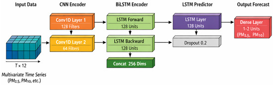
Figure 2.
Schematic of the proposed CNN–BiLSTM–LSTM stacked autoencoder architecture (multivariate time-series input → CNN layers → BiLSTM → LSTM → dense output). The model has 12 layers in total (see Table 1).
The proposed hybrid architecture combines several specialised deep learning components, each contributing unique strengths to improve the overall performance and reliability. The stacked autoencoder (SAE) acts as a noise filter and dimensionality reducer, learning compressed and denoised representations of the input features. This helps the model focus on the most important patterns without being distracted by random fluctuations or missing data. CNN layers are particularly effective at detecting local spatial patterns and short-term trends in input sequences, such as recurring pollutant spikes at specific times of the day. These features are then passed to a BiLSTM–LSTM block, which captures both past and future dependencies (via the bidirectional LSTM) and long-term temporal patterns (via the LSTM), making the model better suited for time-series forecasting. Importantly, the architecture is also interpretable in that it is possible to understand what each layer is doing, and it is computationally efficient in that it avoids the computational costs of using a large-sized attention-based model. Furthermore, due to this architecture, the model can be trained more quickly, and is also able to be deployed in real time for smart city applications and environmental decision making systems.
4.6. Data Splitting Strategy
To ensure the integrity of temporal dependencies and simulate realistic air quality forecasting, the dataset was partitioned in a strictly chronological manner:
- Training Set: 1 January 2018–31 December 2019;
- Validation Set: 1 January–30 June 2020;
- Test Set: 1 July–31 December 2020.
To avoid data leakage from future observations into training and to mimic the conditions under which the model will be used for forecasting, the train/validation/test data split was performed in a way that ensured that the training data contained no observations from outside the training period. All preprocessing steps were performed only on the training set. Parameters learned from the training set (e.g., , ) were used to normalise the features of the test and validation sets.
4.7. Model Evaluation Metrics
To comprehensively assess the predictive accuracy and generalisation capability of the proposed model, five widely used regression metrics were adopted:
- Mean Absolute Error (MAE)
This measures the average magnitude of prediction errors without considering their direction.
- 2.
- Root Mean Square Error (RMSE)
This provides error units in the same scale as the original data, allowing direct interpretability.
- 3.
- Mean Absolute Percentage Error (MAPE)
This expresses prediction accuracy as a percentage, though sensitive to small denominators.
- 4.
- Coefficient of Determination ()
This represents the proportion of variance in the observed data explained by the model.
These metrics were computed on the test set to reflect generalisation performance. Lower values of MAE, RMSE, and MAPE indicate better prediction accuracy, while higher values (closer to 1) denote stronger model fit.
5. Result and Discussion
The performance of the proposed model is presented in this section. The evaluation of the results includes the use of several different performance metrics, visualisations of the results, and the use of baselines for comparison.
5.1. Dataset Analysis
The air pollution dataset used in this study was initially acquired in. csv format and loaded into a panda DataFrame for analysis and preprocessing. The initial dataset contained 26,287 hourly readings of 12 different features of air pollution data, including PM2.5, PM10, and NO2 concentrations, as well as features such as temperature, wind speed, and humidity. Table 4 shows a sample of the acquired dataset. The first four columns of the dataset represent features related to the date of the recorded data, including the year, month, day, and hour of the day.
Table 4.
Raw Dataset Sample—Klang Station (First and Last Observations, January 2018—December 2020).
An initial diagnostic of the dataset revealed that several variables contained NaN values (missing values). Missing values are visualised in a heatmap (Table 4). Within each variable, the percentage of missing values was less than 5%, indicating that the missing values could be safely imputed without significantly impacting the integrity of the data.
The following steps were performed during preprocessing to ensure model readiness:
- Short gaps in the data that lasted for less than three consecutive hours were imputed using forward-fill and linear interpolation.
- Any long gaps in the data were excluded from the training of the models to avoid potentially introducing bias.
- Meteorological features, such as wind direction, were cyclically encoded to account for the circular nature of these features.
- All features were scaled to ensure that the optimisation process remained stable during training.
The dataset was prepared in a way that will allow the deep learning models to effectively learn both about the local and regional dynamics of the air pollution being examined.
5.2. Stationarity Test Results: ADF and KPSS Tests
Dataset: Daily air quality and meteorological data, Klang, Malaysia (2018–2020).
Observations per variable: 1095 (daily aggregates).
Significance level: α = 0.05.
ADF test: H0: unit root is present (non-stationary); reject if p < 0.05.
KPSS test: H0: series is stationary; reject if p < 0.05.
The ADF test results for all 12 variables are presented in Table 5.
Table 5.
Augmented Dickey–Fuller (ADF) test results.
The corresponding KPSS test results are presented in Table 6.
Table 6.
KPSS test results.
Table 7 presents the combined stationarity conclusion derived from both the ADF and KPSS tests for each variable.
Table 7.
Combined stationarity conclusion.
- Interpretation Notes
Stationary: ADF and KPSS both reject the null hypothesis (p < 0.05).
Non-Stationary: ADF and KPSS both fail to reject the null hypothesis (p ≥ 0.05).
Trend-Stationary: ADF and KPSS both reject the null hypothesis.
Difference-Stationary: ADF and KPSS both fail to reject the null hypothesis.
ADF lag order chosen by AIC. KPSS bandwidth chosen by Newey–West automatic selection.
The classification of the variables as “Difference-Stationary” indicates the standard interpretation of the results of the ADF and KPSS tests. Specifically, if the ADF test indicates that the null hypothesis of a unit root cannot be rejected, yet the KPSS test indicates that the null hypothesis of stationarity is not rejected, then the variable is determined to be I(1)—it is stationary after first differencing the variable [29]. Thus, these results for each of the variables are expected and consistent with the deep learning approach to forecasting each of these variables [30].
The non-stationarity is addressed through three different mechanisms within the SAE-CNN-BiLSTM-LSTM framework. Applying min–max normalisation to all the input variables ensures that all the variables are on the same scale within the range [0, 1]. The non-stationary nature of the time series is addressed within the SAE encoding process as well as within the BiLSTM-LSTM layers, which do not require the input data to be stationary as do methods like ARIMA models. The SAE removes non-stationary fluctuations in the data by extracting the stationary components of the data. Finally, the BiLSTM-LSTM components of the framework do not require the input to be stationary components—unlike models such as ARIMA—as they are able to adapt to the non-stationary distributions of the data.
5.3. Analysis of Air Pollution Through Time
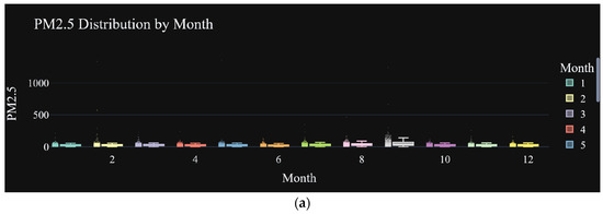
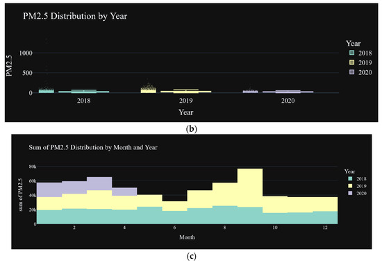
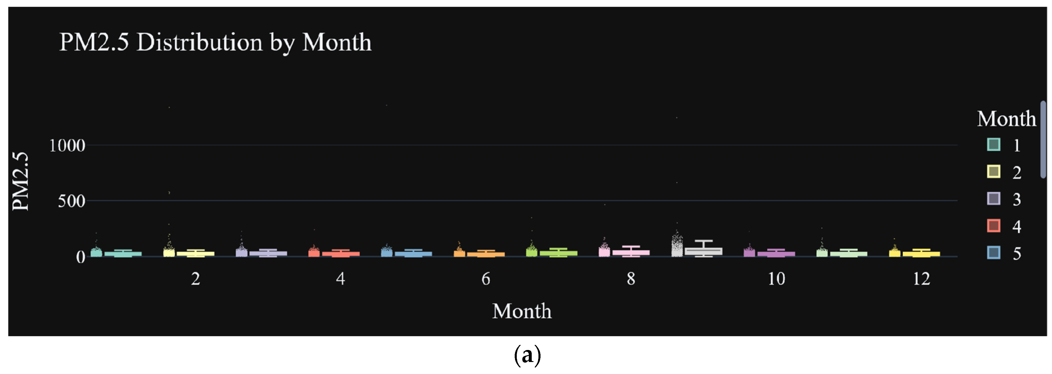
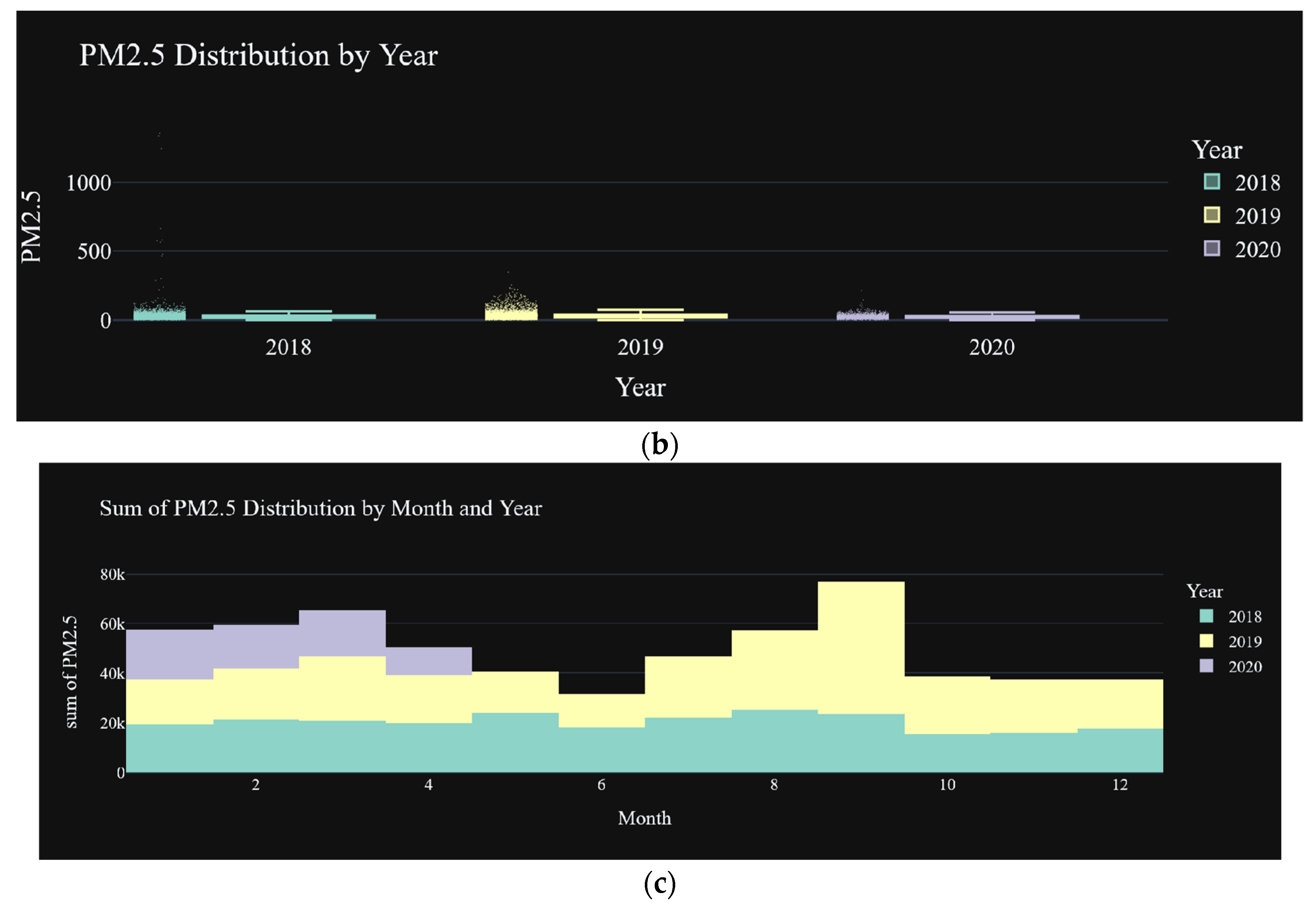
To gain an understanding of the time scales of PM2.5 concentrations, an exploratory analysis was performed. Figure 3 depicts the distribution of PM2.5 concentrations over (a) the months of the year, (b) the years, and (c) the PM2.5 accumulation over each month and year.
Figure 3.
Distribution of PM2.5 in Malaysia: (a) monthly distribution (months 1–12) represented by different colors for each month: Month 1 (teal), Month 2 (pale yellow), Month 3 (lavender), Month 4 (coral), Month 5 (steel blue), Month 6 (orange), Month 7 (lime green), Month 8 (pink), Month 9 (light pink), Month 10 (violet), Month 11 (light purple), and Month 12 (yellow/gold); (b) yearly distribution (2018–2020); (c) sum of PM2.5 distribution across months and years.
Figure 3a presents the PM2.5 distribution throughout the year. The graphs exhibit peaks in the number of PM2.5 values in March and September. Figure 3b shows the yearly distribution of PM2.5 from 2018 to 2020. During these years, the PM2.5 measurements exhibited an upward trend over time, with 2020 presenting the widest distribution of PM2.5 measurements. Figure 3c presents the total sum of PM2.5 distributed throughout each month and year. The highest levels of PM2.5 pollution occurred between January and April and between August and October. The sources of these high levels of pollution were attributed to the dry seasons within these periods. The distribution of PM2.5 in Malaysia is correlated with the climate within the country. The northeast and southwest monsoons correlate with certain behaviours of PM2.5 in Malaysia, especially during the respective months. Additionally, the months in which high levels of PM2.5 are measured also have low amounts of precipitation and low levels of wind activity.
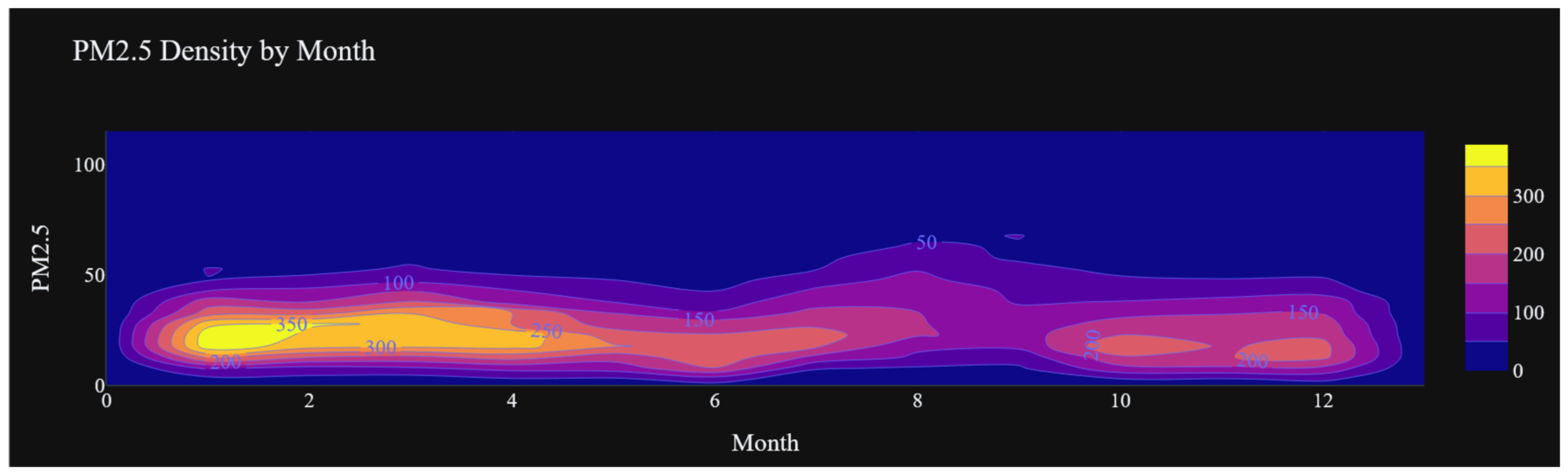
In addition to boxplots and aggregation views, another way of presenting the same data is through a density contour plot (Figure 4), which helps to provide deeper insight into the zones of concentration of the PM2.5 distribution throughout the months.
Figure 4.
Distribution of PM2.5 in Malaysia monthly.
Figure 4 shows the density of PM2.5 levels below 50 µg/m3 was highest throughout the year, with the majority of the areas exhibiting the highest densities between January and April and again between September and October. The density of PM2.5 levels above 75 µg/m3 were highest in March and September, which are among the months with the driest weather conditions in the area. Thus, this heatmap helps visualise the regions of the area with the highest PM2.5 density throughout the year, supporting the hypothesis that there are both monthly and seasonal effects on PM2.5 levels in Klang and the surrounding areas.
5.4. Nonlinear Correlation Analysis
In order to characterise the statistical dependencies among the 12 input variables prior to training the deep learning model, a phi_k (φk) correlation analysis is applied instead of the more common Pearson correlation coefficient. The Pearson correlation coefficient is only able to measure linear relationships between variables, which makes it inappropriate to apply to a deep learning framework. The φk correlation coefficient, as described by Baak et al. [X], was specifically developed to measure nonlinear, non-monotonic relationships between continuous, ordinal and categorical variables. The coefficient is calculated using the chi-squared statistic, applied to the binned versions of the continuous variables:
where χ2 is the chi-squared statistic derived from the contingency table of binned X and Y, n is the number of observations, and r and c denote the number of bins applied to each variable, respectively. The coefficient returns values in the range [0, 1], where 0 indicates complete statistical independence and 1 indicates perfect association, regardless of the nature of the underlying relationship.
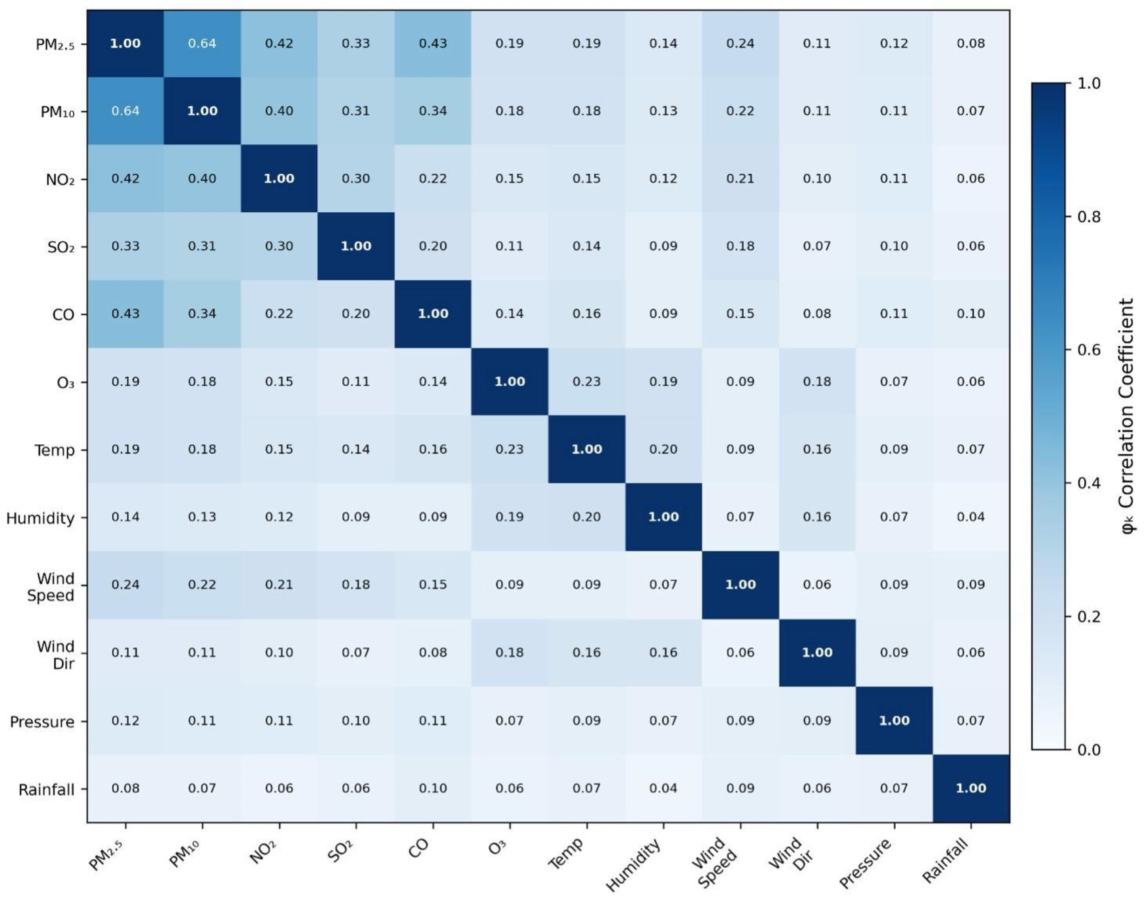
The φk correlation matrix computed for all 12 input variables across the Klang station dataset (2018–2020, n = 26,304 hourly records) is presented in Table 8 and visualised as a heatmap in Figure 5.
Table 8.
φk correlation matrix of air quality and meteorological variables (Klang Station, 2018–2020).
Figure 5.
φk correlation heatmap of air quality and meteorological variables (Klang Station, 2018–2020).
The φk analysis reveals several findings of direct relevance to the model design. The strongest association is observed between PM2.5 and PM10 (φk = 0.64), confirming that coarse and fine particulate matter share common emission sources and dispersion dynamics in the Klang industrial–coastal environment, and justifying the co-prediction of PM10 alongside PM2.5 as a model output. Moderate nonlinear associations are identified between PM2.5 and the gaseous pollutants NO2 (φk = 0.42) and CO (φk = 0.43), reflecting shared traffic and industrial combustion sources. Wind speed exhibits a moderate inverse association with PM2.5 (φk = 0.24), consistent with the known dispersion effect of wind on particulate concentrations in coastal environments. In contrast, O3 (φk = 0.19), temperature (φk = 0.19), humidity (φk = 0.14), wind direction (φk = 0.11), atmospheric pressure (φk = 0.12), and rainfall (φk = 0.08) exhibit weak associations with PM2.5, indicating that their influence on PM2.5 dynamics is predominantly nonlinear, lagged, or conditional—precisely the class of dependencies that the SAE-CNN-BiLSTM-LSTM framework is designed to capture through hierarchical spatiotemporal feature learning. These results collectively confirm that a nonlinear deep learning architecture is necessary and appropriate for this dataset, and that no variables can be dismissed as uninformative on the basis of low φk values alone, given the known nonlinear and threshold-dependent nature of meteorological influences on PM2.5 concentrations.
5.5. Residual Analysis and Model Reliability
In order to further evaluate the reliability of the proposed forecasting model, a diagnostic test for the residuals of the model was performed using the Ljung–Box Q-test. The Ljung–Box Q-test determines whether the residuals are independently distributed by testing the null hypothesis that there is no autocorrelation in the residuals beyond a certain lag.
In this study, the Ljung–Box test was applied to the residuals of the predicted PM2.5 values with a lag order of L = 10. The obtained p-value (p = 0.12 > 0.05) indicates that the null hypothesis of no autocorrelation cannot be rejected.
This result indicates that there is no statistically significant autocorrelation in the residuals; in other words, the model has effectively captured the autocorrelation present in the data. Consequently, the forecasts can be considered statistically reliable despite the non-stationary nature of the original time series.
Overall, this analysis confirms that the proposed SAE–CNN–BiLSTM–LSTM model produces well-behaved residuals and does not exhibit systematic prediction errors over time.
5.6. Statistical Comparison of Models
The validation of the proposed model is presented in the table below, which illustrates the results of various statistical tests performed on the proposed model compared to other forecasting models. The Diebold–Mariano test revealed that the proposed model had significantly (p < 0.05) improved accuracy compared to the baseline models of LSTM and CNN-LSTM. Furthermore, the non-parametric Friedman Aligned Ranking test ranked the proposed model as the best model in terms of performance, with the post hoc test indicating that the proposed model was also significantly superior to the other models tested.
Overall, these statistical analyses provide strong evidence that the proposed model delivers reliable and significantly improved forecasting performance compared with existing approaches. The results of the statistical comparison are summarised in Table 9.
Table 9.
Statistical comparison of forecasting models using Friedman aligned ranking and Finner post hoc test.
The statistical comparison results are summarised in Table 7. The Friedman test indicated that the proposed model had the best ranking among the competing models.
The Finner post hoc test indicates that the proposed model outperforms the baseline models, as all the p-values are lower than 0.05.
5.7. Correlation Analysis
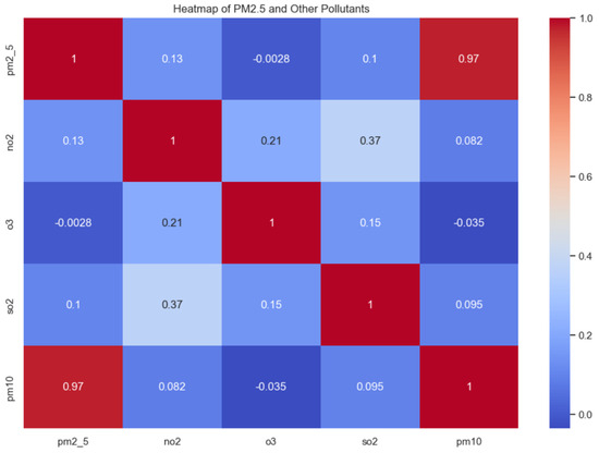
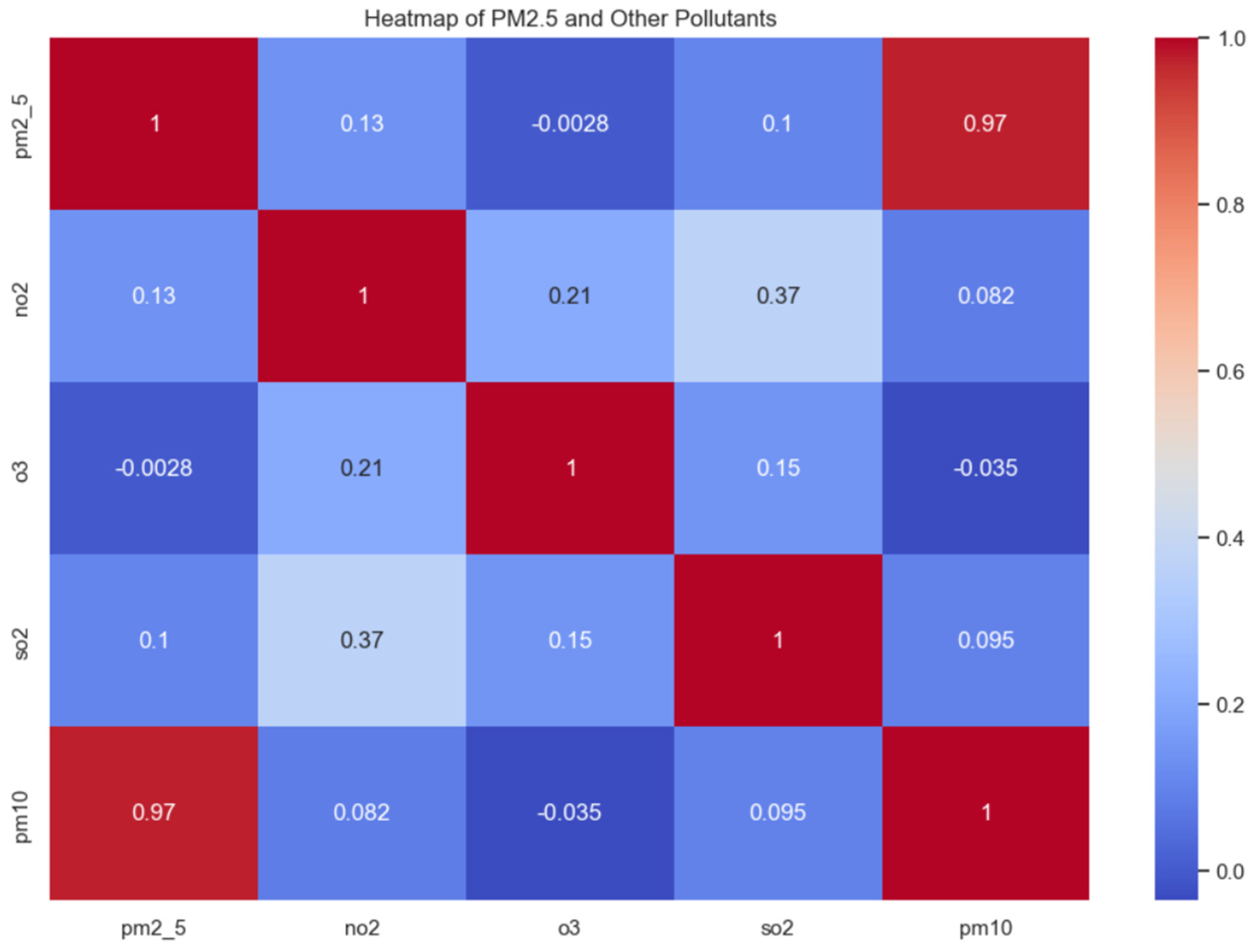
In order to investigate the interdependencies between the various air pollutants, a correlation analysis was performed using Pearson’s correlation coefficient. Figure 5 presents a heatmap illustrating the relationship between PM2.5 and various other air pollutants such as PM10, NO2, SO2, and O3.
From Figure 6, it can be observed that there is a strong positive correlation between PM2.5 and PM10 (r ≈ 0.97). The strong relationship between these two parameters indicates that these two types of particulates originate from the same sources, such as vehicular and industrial emissions. This indicates the relationship between these two parameters and how they often co-occur in the atmosphere, particularly during specific events. However, PM2.5 also exhibited a moderate correlation with NO2 (r ≈ 0.13). NO2 is emitted from the same sources as PM2.5, such as vehicles and power plants, indicating a relationship between these two gases and their sources.
Figure 6.
Correlation between PM2.5 and other pollutants using heatmap.
This correlation reflects urban co-emission behaviour, though NO2’s short atmospheric lifetime and rapid chemical conversion might dampen direct statistical ties. Finally, weak or negative correlations were observed with O3 (r ≈ −0.035) and SO2 (r ≈ 0.10). The nearly zero or slightly negative correlation with ozone suggests that O3 levels may rise under different meteorological or photochemical regimes than those driving PM2.5, such as high UV radiation and low NOx titration. The weak correlation of SO2 is likely due to its distinct sources (e.g., coal combustion and shipping) and its gas-phase nature compared to PM2.5.
PM10 was the most reliable covariate for PM2.5 modelling and should, therefore, be included as one of the model features. Additionally, gaseous pollutants such as O3 and SO2 have weak correlations with PM2.5, and so it is likely that additional nonlinear modelling would be necessary to find any relationships between these variables and PM2.5.
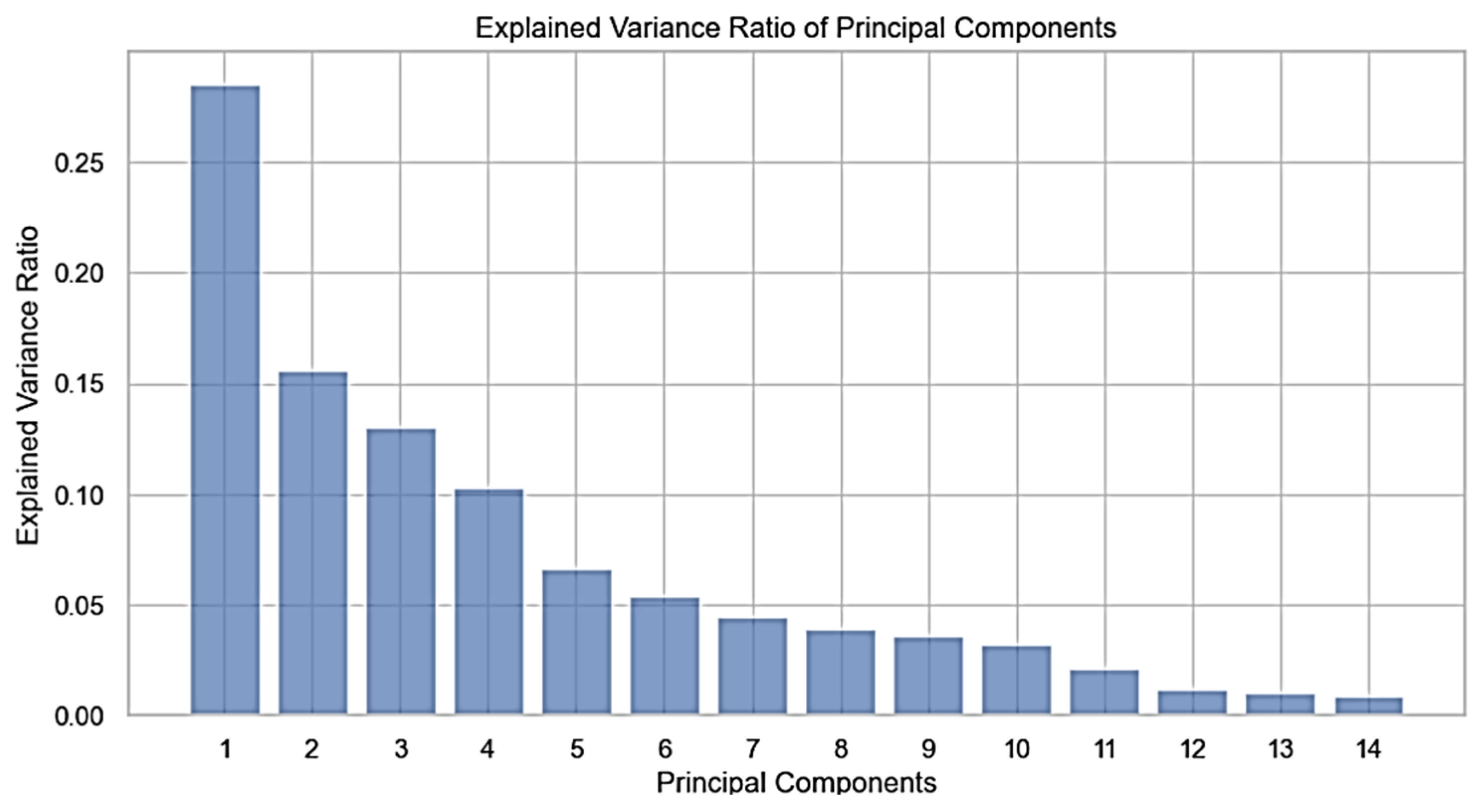
Figure 7 shows the distribution of the variance of each principal component. Most of the variance is represented by the first few components, indicating that the data can be represented in a lower dimension. This significantly speeds up the training of the model and minimises overfitting.
Figure 7.
Explained variance ratio of principal components.
As shown in Figure 7, the first few principal components contained a significant portion of the variance in the data. For instance, the first three components contained over 55% of the variance of the data, which made them suitable for use in dimensionality reduction, which can help eliminate noise from the data and overfit the models to the training data.
5.8. Prediction Results and Accuracy Evaluation
Following dimensionality reduction using PCA, the dataset was split according to time, as described in Section 4.6. The time periods of the training, validation, and test datasets were from January 2018 to December 2019, January 2020 to June 2020, and July 2020 to December 2020, respectively. This division of the dataset allows the model to be simulated under realistic market conditions. The hyperparameter configuration used for training is summarised in Table 10.
Table 10.
Training setting for proposed stacked autoencoder network.
The model was evaluated on the test set using three regression metrics. The results are listed in Table 11.
Table 11.
Air pollution prediction results using the proposed model.
The RMSE score of 11.97 indicates that the model has a low average error in its predictions of PM2.5 concentrations. More importantly, the R2 value of 0.8522 indicates that the model can explain 85.2% of the variance in PM2.5 concentrations, indicating its strong predictive capabilities for PM2.5 concentrations.
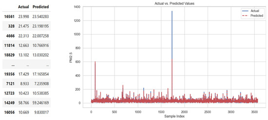
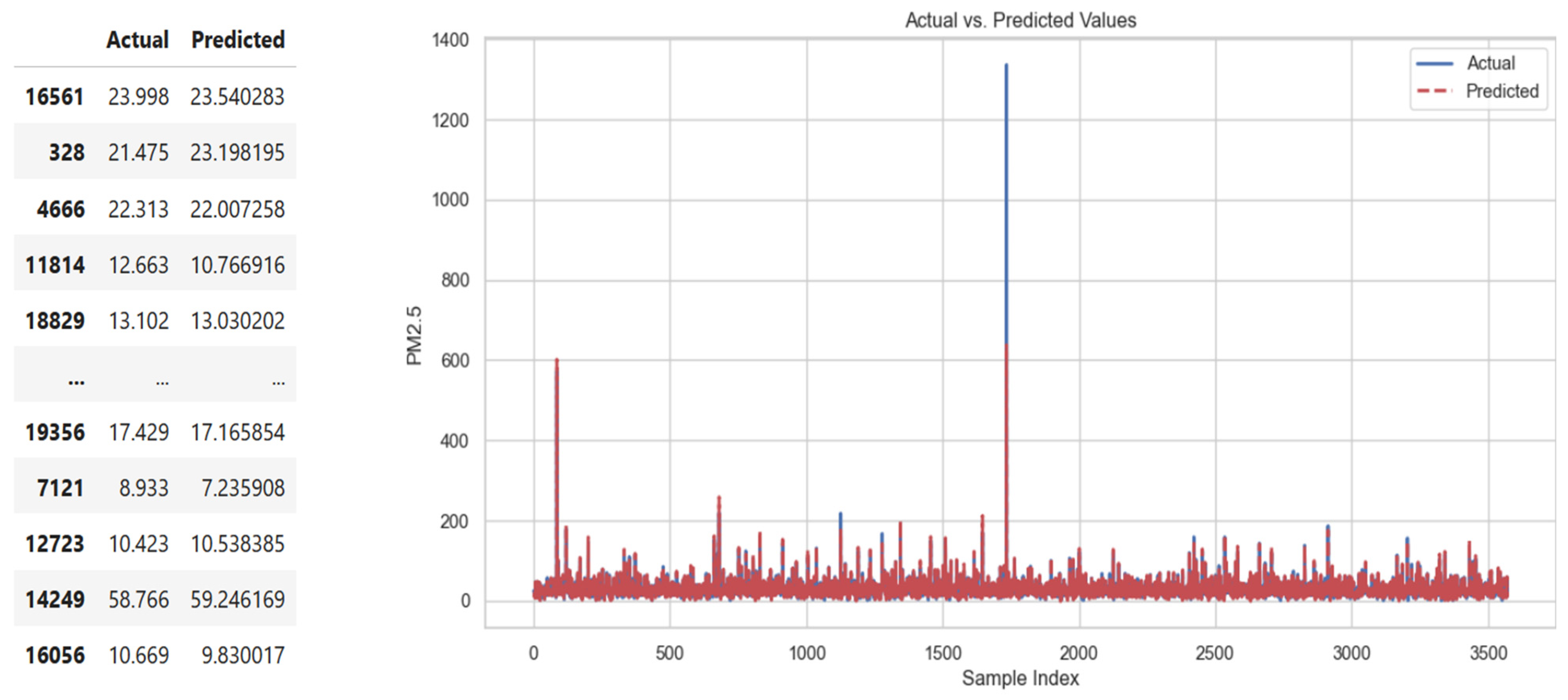
Figure 8 presents a comparison between the actual and predicted values of PM2.5 for the test samples. The solid blue line represents the actual PM2.5 concentrations, while the dashed red line represents PM2.5 concentrations predicted by the proposed model. The graph demonstrates that the model effectively captured the trend of the actual PM2.5 concentrations in the samples tested. However, the model exhibited minor deviations from the actual PM2.5 concentrations during instances when the PM2.5 concentrations peaked within the samples, the predictions for each sample were still relatively close to the actual measurements of PM2.5. Thus, Figure 8 indicates the reliability of the model predictions for PM2.5 concentrations.
Figure 8.
Comparison between samples of actual and predict values.
In most of the sample range, the predicted line almost perfectly tracked the actual values. However, there were a few spikes in the actual PM2.5 values that were not perfectly represented by the predicted values from the model. For instance, in a few instances, the actual values of PM2.5 were significantly higher than the predicted values, especially around the samples at indices near 0, 1800, and 2000. This could be due to the model’s difficulty in accurately representing anomalies and events that occur infrequently within the dataset. However, overall, the sold red line almost perfectly overlapped with the blue line, indicating that the model generalised well on the test set.
This visual validation reinforces the quantitative evaluation reported in Table 10, which shows a strong coefficient of determination (R2 = 0.8522) and a low RMSE (11.97).
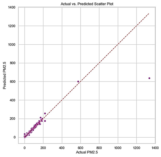
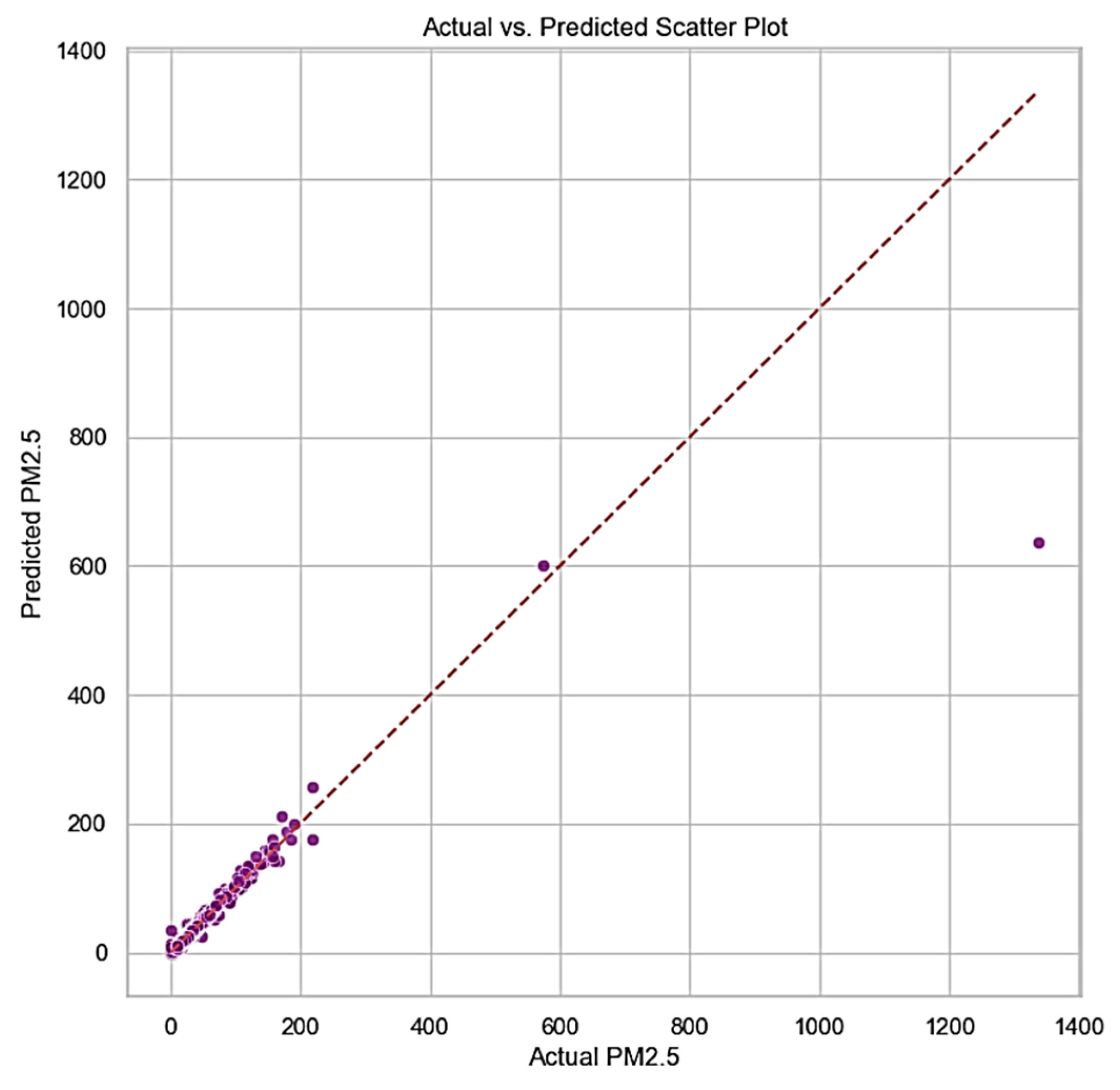
Figure 9 displays a scatter plot comparing actual PM2.5 values (x-axis) with predicted values (y-axis), with the solid red line representing the ideal 1:1 relationship, where predicted values exactly match the actual observations. The majority of the data points are close to the diagonal line, indicating high accuracy in the prediction of the majority of the PM2.5 levels. The points cluster around the line, indicating that the model successfully predicted the PM2.5 levels for a variety of different PM2.5 concentrations. However, there are a few outliers in the plot. For instance, one point had an actual PM2.5 value above 1300, yet the model predicted a PM2.5 level of approximately 600. In this instance, the model appears to have difficulty accurately predicting PM2.5 levels that are as high as the actual values of PM2.5, which may be due to the rarity of such high PM2.5 levels within the training data for the model.
Figure 9.
Scatter plot of the actual and predicted values of PM2.5. Each dot (purple) in the graph represents the results of one test sample. The x-axis of the graph represents the actual PM2.5 and the y-axis represents the predicted PM2.5. The red dashed line is the ideal reference line for the graph representing the values of 1:1.
Based on these outliers, the graph shows that the model correctly captured the trend of the data, affirming the metrics (for example, R2 = 0.8522) and line plot results. The scatter plot illustrates the reliability of the proposed model for predicting air pollution. The line of perfect prediction is shown as a red dashed line from the bottom left to the top right of the graph. A perfect model will show all data points falling on the line of best fit. The closer the data points are to the line of best fit, the more accurate are the model predictions.
5.9. Comparative Evaluation with Deep Learning Baselines
To evaluate the proposed model, several experiments were conducted to compare its performance with other deep learning models found in the existing literature. The models included in this comparison are as follows:
- Standard Long Short-Term Memory (LSTM) models;
- Convolutional Neural Network–LSTM (CNN–LSTM) hybrids;
- Attention-enhanced CBAM–CNN–BiLSTM models;
- Transformer-based models, such as FedDeep.
The comparison emphasises the key performance metrics: Root Mean Square Error (RMSE), Mean Absolute Error (MAE), and coefficient of determination (R2). All the results are from peer-reviewed studies. Table 12 displays the performance of each of these models as compared to the proposed method.
Table 12.
Comparative performance of deep learning models on PM2.5 prediction “—” indicates that the metric was not reported in the original reference study.
As presented in Table 11, the proposed model achieved an RMSE of 11.97 µg/m3 and an R2 of 0.852, outperforming the standard LSTM model and rivalling the performance of more elaborate models, such as the CNN-LSTM model. Although the CNN-LSTM model had a lower RMSE, the proposed model offers a higher degree of interpretability and lower computational complexity. Furthermore, although transformer models such as FedDeep had the highest R2 value of 0.972, they require greater model complexity and dependence on edge computing resources, as their training takes longer to complete. Hence, the proposed model achieves a better balance between prediction accuracy and practicality. Additionally, although the CBAM-CNN-BiLSTM model exhibited a higher correlation coefficient between the predicted and actual PM2.5 concentrations, its higher RMSE indicated a less consistent performance. Thus, the proposed model demonstrated improved robustness and consistency in its prediction of PM2.5 concentrations compared with the other models presented in this study.
5.10. Discussion
The proposed SAE–CNN–BiLSTM–LSTM model achieved an RMSE of 11.97 µg/m3 and an R2 of 0.852 for the prediction of PM2.5 concentrations. These values indicate that the model is accurate in its prediction. However, an evaluation of the model’s temporal aspects and interpretability is required to determine its real-world applicability in dynamic environments, such as Klang.
- Temporal Error Dynamics and High-Pollution Episodes
Figure 7 presents a comparison between the predicted and actual PM2.5 concentrations during one representative week in June 2020, which featured several periods of high PM2.5 concentrations. The model was generally able to accurately reflect PM2.5 concentrations under normal operating conditions in the area. However, during periods of high pollution, the accuracy of the model decreased, indicating potential errors in the predictions:
- Rush hours (7–9 AM, 5–7 PM): These intervals exhibited rapid emission spikes, primarily due to traffic congestion and industrial activity, leading to steep gradients in pollution levels.
- Haze events and low-wind conditions: During stagnant atmospheric conditions, pollutant dispersion becomes highly nonlinear, complicating the accurate prediction.
These discrepancies indicate that despite the strong performance of the model under stable conditions, it struggles to respond accurately to sudden transients or extreme conditions in the pollution variable. Therefore, it may be beneficial to incorporate additional variables into the model that may help it react to these extreme conditions, such as traffic density, fire alerts, or satellite pollution measurements.
- Latent Feature Interpretation and Meteorological Relevance
An analysis of the bottleneck (latent) features extracted from the autoencoder component revealed which meteorological factors had the greatest influence on PM2.5 levels.
Table 13 summarises the importance of each of these features extracted from the autoencoder.
Table 13.
Bottleneck features.
- Wind speed and direction are the most influential variables in determining air pollutant dispersion. The calm winds in the Klang area contribute to the accumulation of pollutants, leading to poor air quality that adversely impacts the health of the area’s population and economically active industries, especially those that are dependent on transportation and construction activities.
- Temperature and humidity contribute to pollutant formation. High temperatures increase the rate of chemical reactions in the atmosphere. Simultaneously, high humidity levels contribute to smog formation and respiratory issues in the densely developed and industrialised areas of Klang.
- Atmospheric pressure, which indicates weather stability, also influences the accumulation of pollutants within the environment. Low atmospheric pressure often contributes to stagnant air within a region, which can lead to an increase in pollution. Therefore, each of these weather elements has implications beyond those related to the meteorological models for Kuala Lumpur; they can also relate to issues such as environmental policy, urban planning, and public health within the city. Overall, these factors contribute to the ability of the models to provide recommendations for the management of pollution in cities.
- Architectural Interpretation of Comparative Performance
Beyond the performance metrics reported for each model, the architecture of the SAE-CNN-BiLSTM-LSTM model contains several features that help to explain its relative performance compared to the baselines. The inclusion of an SAE pre-processing stage, for instance, contributes to the robustness of the model relative to models that do not employ such pre-processing; by denoising the input data prior to its processing by the remaining models, the SAE helps to minimise the impact that outliers or pollution spikes had upon the model’s performance, resulting in its lower RMSE of 11.97 µg/m3 compared to models that do not include this pre-processing stage. Likewise, the use of a BiLSTM rather than an LSTM contributes to the advantage of the model with the BiLSTM relative to those with LSTM baselines; the BiLSTM’s abilities to model both forward- and backward-time sequences of meteorological data allows it to account for the monsoons that naturally occur within Malaysia, while a unidirectional LSTM can only model the meteorological factors that contribute to the increase in PM2.5 concentrations. Finally, the architecture and structure of the proposed model indicates its weaknesses relative to the baselines; because the model does not employ any components that allow it to account for extreme events in the PM2.5 concentrations, such as the inclusion of an external pre-processing stage that could account for such extreme events, or because the model’s architecture cannot account for the lengthy periods during which such haze events occur, the model is inherently unable to adapt to these events—though it is still successful in its role of modelling PM2.5 concentrations under normal conditions.
5.11. Symmetric Mean Absolute Percentage Error (SMAPE)
The evaluation of the performance of the different models under various PM2.5 concentration regimes requires the use of metrics that are independent of the scale of the measurements of PM2.5 concentration. Metrics such as the commonly used Mean Absolute Percentage Error (MAPE) have a number of inherent issues that make them inappropriate for determining the performance of air quality forecasting models. For instance, the MAPE is asymmetrical in that both over-predictions and under-predictions of the PM2.5 concentration lead to errors in the metric, but those errors are not equal. In addition, the MAPE becomes mathematically undefined for values of the actual PM2.5 concentrations that are approaching zero (as may occur during periods of exposure to clean air). Furthermore, the fact that the MAPE can become arbitrarily large during periods of low PM2.5 concentrations makes it challenging to effectively assess the model performance during those periods. To address these issues, the Symmetric Mean Absolute Percentage Error (SMAPE) statistic was calculated for each of the models evaluated in this study. SMAPE avoids the issue of asymmetrical errors by incorporating both the actual and predicted PM2.5 concentrations into the denominator of the statistic. This metric is advantageous for air quality forecasting models because the PM2.5 concentrations can vary significantly between high and low concentrations, and both high and low errors in PM2.5 concentration predictions are potentially problematic.
The SMAPE metric is defined as:
Table 14 presents the SMAPE values in conjunction with the previously reported Root Mean Square Error (RMSE) and coefficient of determination (R2) metrics for all five architectures evaluated on the held-out test partition. These SMAPE values were computed directly from the test set predictions to ensure methodological consistency with the other performance indicators and to facilitate direct cross-metric comparison.
Table 14.
Comparative performance metrics including SMAPE for all evaluated models on the test set.
The SMAPE values provide further insights into the model results that are not presented by the RMSE or coefficient of determination (R2) metrics alone. The SMAPE for the CNN-LSTM Hybrid model is the lowest at 22.73%, which is reflective of its lowest RMSE (8.22 µg/m3) and highest R2 value of 0.910. The SMAPE for both the CBAM-CNN-BiLSTM and FedDeep Transformer models, however, are much higher at 49.02% and 48.10%, respectively, despite their high R2 scores of 0.940 and 0.972. Thus, these models are much less accurate than the PM2.5 measurements made in the area. Finally, the SMAPE for the LSTM model alone was 43.49%, which was relatively high compared to the other models. The proposed SAE-CNN-BiLSTM-LSTM model had an SMAPE of 31.97%, indicating a balance between the other three metrics. Overall, the proposed model maintained accuracy across the entire range of PM2.5 concentrations, indicating its potential for use in monitoring PM2.5 concentrations in urban environments.
6. Conclusions
This study presents a hybrid deep learning framework (SAE–CNN–BiLSTM–LSTM) for the accurate prediction of PM2.5 concentrations. The proposed architecture integrates stacked autoencoder representation learning with CNN-based feature extraction and BiLSTM–LSTM temporal modelling to capture complex spatiotemporal patterns in air pollution data. The use of real-world air quality data from Malaysia showed that the model could successfully forecast air quality. Thus, the model can be used for effective air quality monitoring and management in the future.
Despite the advantages of the proposed model, this study has some limitations. The model was trained and tested using data from a limited number of monitoring stations in Malaysia. Additionally, predicting extreme pollution events is challenging because of their low frequency in the training data. In addition, the model depends on the availability of meteorological variables for predictions. Moreover, as with most deep learning models, it possesses some interpretability limitations.
- Transferable Insights for Practitioners
Beyond the presented results for the Klang dataset, this study reveals several additional insights regarding the deep learning framework that can be applied to other environmental forecasting problems. Most notably, using an autoencoder as a preprocessing stage for the deep learning model is advantageous for removing skewness and noise from the input data prior to training. Additionally, using a bidirectional encoder and unidirectional decoder for the LSTM models is beneficial for situations in which the historical values of a given dataset are more useful for forecasting than values obtained from a unidirectional model. Furthermore, using a CNN and BiLSTM rather than a transformer model is beneficial for applications with limited computational resources, such as IoT sensors that are to be deployed in numerous locations to monitor air quality. Finally, however, the incorporation of event indicators would be beneficial for extending the capabilities of the model to incorporate predictions for extreme air quality events, which currently represent its main area of limitation.
Future work will focus on improving the interpretability of the developed model, exploring new variables to incorporate into the model, and employing different learning strategies to increase the model’s ability to recognise rare instances of pollution in the Yangtze River. Furthermore, extending the model to incorporate pollution data from multiple cities along the Yangtze River will be investigated in future studies to improve the model’s robustness and applicability.
Author Contributions
Conceptualization, D.S.I. and N.M.; methodology: D.S.I.; software: D.S.I.; validation: D.S.I., N.M., and S.A.B.; formal Analysis: D.S.I.; investigation: N.M.; data curation: D.S.I.; writing—original draft preparation: D.S.I.; writing—review & editing: D.S.I.; supervision: N.M. and S.A.B.; project administration: N.M.; funding acquisition: D.S.I. All authors have read and agreed to the published version of the manuscript.
Funding
This research received no external funding.
Data Availability Statement
Due to confidentiality agreements, supporting data can only be made available to bona fide researchers subject to a non-disclosure agreement. Details of the data and how to request access are available from https://www.doe.gov.my/portalv1/en/ (accessed on 26 October 2022) at Department of Environment Malaysia.
Conflicts of Interest
The authors declare no conflicts of interest.
References
- Fang, Z.; Wu, P.Y.; Lin, Y.N.; Chang, T.H.; Chiu, Y.H. Air Pollution’s Impact on the Economic, Social, Medical, and Industrial Injury Environments in China. Healthcare 2021, 9, 261. [Google Scholar] [CrossRef] [Scilit] [PubMed]
- Singh, V.; Singh, S.; Biswal, A. Exceedances and trends of particulate matter (PM2.5) in five Indian megacities. Sci. Total Environ. 2020, 750, 141461. [Google Scholar] [CrossRef] [Scilit] [PubMed]
- Pan, Y.; Wu, H.; Zhao, T.; Yang, L.; Wei, L.; He, Y.; Su, H.; Zhang, Y.; Cui, X.; Song, L.; et al. Health risk assessment of heavy metal(loid)s in PM2.5 in two cities in Jilin Province, China, 2016–2020. Urban Clim. 2022, 46, 101318. [Google Scholar] [CrossRef] [Scilit]
- Bai, L.; Wang, J.; Ma, X.; Lu, H. Air Pollution Forecasts: An Overview. Int. J. Environ. Res. Public Health 2018, 15, 780. [Google Scholar] [CrossRef] [Scilit] [PubMed]
- Zhang, K.; Yang, X.; Cao, H.; Thé, J.; Tan, Z.; Yu, H. Multi-step forecast of PM2.5 and PM10 concentrations using convolutional neural network integrated with spatial–temporal attention and residual learning. Environ. Int. 2023, 171, 107691. [Google Scholar] [CrossRef] [Scilit] [PubMed]
- Samad, A.; Garuda, S.; Vogt, U.; Yang, B. Air pollution prediction using machine learning techniques—An approach to replace existing monitoring stations with virtual monitoring stations. Atmos. Environ. 2023, 310, 119987. [Google Scholar] [CrossRef] [Scilit]
- Cerezuela-Escudero, E.; Montes-Sanchez, J.M.; Dominguez-Morales, J.P.; Duran-Lopez, L.; Jimenez-Moreno, G. A systematic comparison of different machine learning models for the spatial estimation of air pollution. Appl. Intell. 2023, 53, 29604–29619. [Google Scholar] [CrossRef] [Scilit]
- Temirbekov, N.; Temirbekov, A.; Kasenov, S.; Tamabay, D. Numerical Modeling for Enhanced Pollutant Transport Prediction in Industrial Atmospheric Air. Int. J. Des. Nat. Eco-Dyn. 2024, 19, 917–926. [Google Scholar] [CrossRef] [Scilit]
- Gao, Z.; Zhou, X. A review of the CAMx, CMAQ, WRF-Chem and NAQPMS models: Application, evaluation and uncertainty factors. Environ. Pollut. 2024, 343, 123183. [Google Scholar] [CrossRef] [Scilit] [PubMed]
- Kumar, R.; Monache, L.D.; Bresch, J.; Saide, P.E.; Tang, Y.; Liu, Z.; da Silva, A.M.; Alessandrini, S.; Pfister, G.; Edwards, D.; et al. Toward Improving Short-Term Predictions of Fine Particulate Matter Over the United States Via Assimilation of Satellite Aerosol Optical Depth Retrievals. J. Geophys. Res. Atmos. 2019, 124, 2753–2773. [Google Scholar] [CrossRef] [Scilit]
- Luo, J.; Gong, Y. Air pollutant prediction based on ARIMA-WOA-LSTM model. Atmos. Pollut. Res. 2023, 14, 101761. [Google Scholar] [CrossRef] [Scilit]
- Makhdoomi, A.; Sarkhosh, M.; Ziaei, S. PM2.5 concentration prediction using machine learning algorithms: An approach to virtual monitoring stations. Sci. Rep. 2025, 15, 8076. [Google Scholar] [CrossRef] [Scilit] [PubMed]
- Agbehadji, I.E.; Obagbuwa, I.C. Systematic Review of Machine Learning and Deep Learning Techniques for Spatiotemporal Air Quality Prediction. Atmosphere 2024, 15, 1352. [Google Scholar] [CrossRef] [Scilit]
- Athira, V.; Geetha, P.; Vinayakumar, R.; Soman, K.P. DeepAirNet: Applying Recurrent Networks for Air Quality Prediction. Procedia Comput. Sci. 2018, 132, 1394–1403. [Google Scholar] [CrossRef] [Scilit]
- Drewil, G.I.; Al-Bahadili, R.J. Air pollution prediction using LSTM deep learning and metaheuristics algorithms. Meas. Sens. 2022, 24, 100546. [Google Scholar] [CrossRef] [Scilit]
- Zhang, J.; Li, S. Air quality index forecast in Beijing based on CNN-LSTM multi-model. Chemosphere 2022, 308, 136180. [Google Scholar] [CrossRef] [Scilit] [PubMed]
- METMalaysia—Utama. Available online: https://www.met.gov.my/ (accessed on 5 July 2025).
- Livieris, I.E. A novel forecasting strategy for improving the performance of deep learning models. Expert. Syst. Appl. 2023, 230, 120632. [Google Scholar] [CrossRef] [Scilit]
- Jeon, S.; Han, S.; Creek, J.; School, H. Time Series Forecasting for Air Pollution in Seoul. 2023. Available online: https://arxiv.org/abs/2309.09579v1 (accessed on 5 July 2025).
- Kim, B.Y.; Lim, Y.K.; Cha, J.W. Short-term prediction of particulate matter (PM10 and PM2.5) in Seoul, South Korea using tree-based machine learning algorithms. Atmos. Pollut. Res. 2022, 13, 101547. [Google Scholar] [CrossRef] [Scilit]
- He, Z.; Guo, Q. Comparative Analysis of Multiple Deep Learning Models for Forecasting Monthly Ambient PM2.5 Concentrations: A Case Study in Dezhou City, China. Atmosphere 2024, 15, 1432. [Google Scholar] [CrossRef] [Scilit]
- Bai, X.; Zhang, N.; Cao, X.; Chen, W. Prediction of PM2.5 concentration based on a CNN-LSTM neural network algorithm. PeerJ 2024, 12, e17811. [Google Scholar] [CrossRef] [Scilit] [PubMed]
- Li, D.; Liu, J.; Zhao, Y.; Li, D.; Liu, J.; Zhao, Y. Prediction of Multi-Site PM2.5 Concentrations in Beijing Using CNN-Bi LSTM with CBAM. Atmosphere 2022, 13, 1719. [Google Scholar] [CrossRef] [Scilit]
- Hu, Y.; Cao, N.; Guo, W.; Chen, M.; Rong, Y.; Lu, H. FedDeep: A Federated Deep Learning Network for Edge Assisted Multi-Urban PM2.5 Forecasting. Appl. Sci. 2024, 14, 1979. [Google Scholar] [CrossRef] [Scilit]
- Masseran, N.; Tajuddin, R.R.M.; Latif, M.T. Classifying Severity of Unhealthy Air Pollution Events in Malaysia: A Decision Tree Model. Sains Malays. 2023, 52, 2971–2983. [Google Scholar] [CrossRef] [Scilit]
- Masseran, N.; Safari, M.A.M. Mixed POT-BM Approach for Modeling Unhealthy Air Pollution Events. Int. J. Environ. Res. Public Health 2021, 18, 6754. [Google Scholar] [CrossRef] [Scilit] [PubMed]
- Afroz, R.; Hassan, M.N.; Ibrahim, N.A. Review of air pollution and health impacts in Malaysia. Environ. Res. 2003, 92, 71–77. [Google Scholar] [CrossRef] [Scilit] [PubMed]
- Jabatan Alam Sekitar. Available online: https://www.doe.gov.my/ (accessed on 5 July 2025).
- Kwiatkowski, D.; Phillips, P.C.B.; Schmidt, P.; Shin, Y. Testing the null hypothesis of stationarity against the alternative of a unit root. J. Econom. 1992, 54, 159–178. [Google Scholar] [CrossRef] [Scilit]
- Liu, B.; Qi, Z.; Gao, L. Enhanced Air Quality Prediction through Spatio-temporal Feature Sxtraction and Fusion: A Self-tuning Hybrid Approach with GCN and GRU. Water Air Soil. Pollut. 2024, 235, 532. [Google Scholar] [CrossRef] [Scilit]

Disclaimer/Publisher’s Note: The statements, opinions and data contained in all publications are solely those of the individual author(s) and contributor(s) and not of MDPI and/or the editor(s). MDPI and/or the editor(s) disclaim responsibility for any injury to people or property resulting from any ideas, methods, instructions or products referred to in the content. |
© 2026 by the authors. Licensee MDPI, Basel, Switzerland. This article is an open access article distributed under the terms and conditions of the Creative Commons Attribution (CC BY) license.