Sensorless Current Estimation in Piezoelectric Energy Harvesting Networks Using a Takagi–Sugeno Fuzzy System

Abstract

This paper proposes a sensorless current estimation method for piezoelectric energy harvesting (PEH) systems using a first-order Takagi–Sugeno fuzzy system. Unlike invasive current sensing, the proposed estimator uses only non-invasive measurements: output voltage $V_O$, its derivative ${\dot{V}}_O$, and load resistance $R_L$. The fuzzy rules are initialized directly from the physical equivalent circuit parameters and trained via the ANFIS on a large-scale dataset (78 million samples). The proposed model achieves a mean coefficient of determination $R^2=0.9999$ (95% CI: [0.99989, 0.99991]), root mean square error $\mathrm{RMSE}=3.12\times {10}^{-8}$ A, mean absolute percentage error MAPE = 2.51% (95% CI: [1.98, 3.04]%), and fitness FIT = 98.98%—outperforming multiple linear regression $(R^2=0.9738$ and MAPE = 116.25%) and a shallow neural network with 211 parameters $(R^2=0.9991$ and MAPE = 13.85%) despite having only 170 trainable parameters. Unlike black-box neural networks, the fuzzy model provides interpretable rules whose consequent parameters map directly to physical quantities (effective capacitance $C_p^{\left(\mathrm{eff}\right)}$ and leakage conductance $1/R_p^{\left(\mathrm{eff}\right)}$). The low computational footprint (170 parameters, <5 μs inference, and ≈1.4 kB of memory) makes it suitable for real-time deployment on low-power microcontrollers. These results demonstrate the viability of the proposed approach under controlled laboratory conditions for the single, series, and parallel PEH configurations considered. This work establishes that physically informed fuzzy modeling is a viable, interpretable, and efficient alternative to deep learning for sensorless monitoring in low-power energy harvesting systems.

1. Introduction

The proliferation of the Internet of Things (IoT), Industry 4.0, and autonomous sensing technologies has driven the demand for sustainable, maintenance-free, and low-power energy sources [1]. In this context, piezoelectric energy harvesting (PEH) has emerged as a compelling solution that is capable of converting ambient mechanical vibrations—ubiquitous in industrial machinery, civil infrastructure, human motion and aircraft cabins, where low-frequency components below 200 Hz are significant [2,3,4]—into usable electrical energy. Recent comprehensive reviews have systematically surveyed the state of the art in piezoelectric energy harvesting, covering fundamental transduction mechanisms, interface circuits, and performance enhancement strategies [5]. Concurrently, emerging multi-domain energy harvesting approaches that exploit mode-dependent magneto-mechano-electric coupling have demonstrated new pathways for enhancing power generation and broadening operational bandwidth [6].

PEH systems typically generate power in the range of microwatts to milliwatts, making them ideally suited for wireless sensor networks (WSNs), structural health monitoring (SHM), and wearable electronics, where battery replacement is either impractical or cost-prohibitive [7,8,9].

Despite its promise, accurate and reliable current measurement in PEH systems remains a significant challenge. The harvested electrical quantities are strongly coupled to the mechanical excitation, and traditional measurement methods are inherently invasive. Inserting a sensing element (e.g., a shunt resistor) introduces parasitic impedances and additional energy dissipation, thereby altering the effective electrical load seen by the piezoelectric transducer and disturbing its electromechanical response [2,10]. This perturbation is particularly critical in low-power scenarios, where the sensor’s own consumption can drastically skew measurements and compromise the energy budget of the entire system [11,12]. Consequently, there is growing interest in developing sensorless estimation strategies that can reconstruct the piezoelectric current using only non-invasive measurements, such as voltage and load resistance, without compromising the harvester’s intrinsic dynamics [2,13].

The existing approaches to sensorless current estimation in PEH systems can be broadly classified into model-driven and data-driven methods. Model-driven methods rely on physics-based electromechanical or equivalent circuit models, such as admittance-based identification [14] or state-space inversion [15]. While interpretable, their accuracy is often limited by parameter uncertainties, unmodeled dynamics, and environmental variations (e.g., temperature). On the other hand, data-driven methods, such as artificial neural networks (ANNs), have recently shown remarkable performance. However, these black-box models present several drawbacks for practical low-power embedded systems: (i) they require large datasets and extensive training; (ii) their high computational complexity demands significant memory and processing power; and (iii) they lack interpretability as the learned mapping remains opaque.

This paper argues that the inherent structure of the PEH system offers an opportunity to overcome these limitations. As shown in [16], the governing equations for single, series, and parallel PEH configurations can be expressed in a unified linear form with respect to five key variables: the output voltage ($V_O$), its temporal derivative ($d{V}_O/dt$), the ratio $V_O/R_L$ (which captures the load-dependent term), the number of parallel elements ($n_p$), and the number of series elements ($n_s$).

This unified linear formulation reveals that a single first-order Takagi–Sugeno fuzzy system with these five inputs can represent all three topologies, eliminating the need for separate models per configuration. This linearity suggests that a complex multi-layer neural network may be an unnecessarily powerful and inefficient tool. Instead, we propose a Takagi–Sugeno (T–S) fuzzy system of order one, which can exactly represent this class of linear relationships while offering the benefits of a gray-box model: high interpretability, low parameter count, and efficient inference [17].

T–S fuzzy systems have been successfully applied to model complex nonlinear processes, such as photosynthesis in agricultural settings [18], and to design robust controllers for overhead cranes [19] and networked systems [20]. Their versatility has also been demonstrated in the modeling and control of other energy harvesting systems, such as triboelectric nanogenerators and electromagnetic generators. Recent advances in these alternative transduction technologies—particularly in wearable biomechanical energy harvesting—have highlighted the potential for applying Takagi–Sugeno fuzzy systems to address their inherent complexities. For instance, hybrid TENG–EMH systems, such as those reported in [21,22], involve multiple nonlinear transduction mechanisms, varying electromechanical coupling conditions, and load-dependent behavior that strongly resemble the challenges addressed in the present work. The structural and parametric complexity of these systems makes them particularly suitable candidates for the application of Takagi–Sugeno fuzzy modeling.

Their ability to combine expert knowledge (or physical laws) with data-driven learning makes them particularly attractive for resource-constrained applications. Unlike neural networks, the rules in a T–S system can be directly initialized from the physical equations (e.g., $i_p=C_p·d{V}_O/dt+V_O/R_{eq}$) and then fine-tuned with data to account for minor nonlinearities or component tolerances. This provides a transparent, auditable, and computationally lean framework for sensorless estimation.

In light of the above, this paper introduces a novel sensorless current estimation framework for PEH networks based on a first-order T–S fuzzy system. The main contributions are:

1.

First T–S Fuzzy Model for PEH Current Estimation: We propose a structured T–S fuzzy model that incorporates the known linear relationships of single, series, and parallel PEH configurations, moving beyond black-box approaches such as neural networks.

2.

Public Large-Scale PEH Database: We introduce and make publicly available a comprehensive dataset comprising over 78 million samples, generated under controlled frequency sweeps (0–200 Hz in 1 Hz steps) and load resistance variations (10–300 kΩ in 5 kΩ steps) for single, series, and parallel configurations of PZT-5J transducers. This database serves as a benchmark for future sensorless estimation research in PEH systems.

3.

Interpretability and Efficiency: We show that the proposed fuzzy model provides clear rule-based insight into the estimation process, a feature that is absent in black-box approaches. Furthermore, its low computational footprint (less than 200 parameters) makes it suitable for real-time implementation on low-power microcontrollers, unlike deep neural networks, which require hundreds of thousands of parameters.

4.

Cross-Topology Validation: The model is validated on single, series, and parallel PEH configurations within a unified framework, demonstrating its ability to accurately estimate the piezoelectric current across all three topologies without requiring topology-specific retraining.

5.

Benchmark for Future Work: The proposed T–S fuzzy model establishes a baseline accuracy against which future sensorless estimation methods can be compared using the publicly released database.

To contextualize the performance of the proposed T–S fuzzy estimator, we establish a comparative framework comprising two baseline methods of increasing complexity. The first baseline is multiple linear regression (MLR), which serves as a reference linear model that ignores the underlying physical structure. Despite its simplicity, MLR reveals the limitations of a purely linear mapping when applied to the unified input space $\{{\dot{V}}_O,V_O,V_O/R_L,n_p,n_s\}$. The second baseline is a shallow neural network (SNN) with a single hidden layer of 30 neurons, totaling 211 trainable parameters—slightly more than the proposed fuzzy model. This architecture was selected to provide a fair comparison against a purely data-driven black-box model of comparable parametric complexity. Both baselines are trained and evaluated on the same random subsample of the dataset (1% of the full 78M samples) to ensure computational feasibility and reproducibility. The comparison demonstrates that the proposed physically informed fuzzy system achieves superior or equivalent accuracy to the neural network while offering full interpretability and lower inference latency and significantly outperforms linear regression across all the metrics.

The remainder of this paper is organized as follows. Section 2 presents the mathematical formulation of the PEH system, the experimental setup, and the dataset generation procedure. Section 3 details the proposed Takagi–Sugeno fuzzy methodology, including the model structure, physical initialization, ANFIS training framework, evaluation metrics, and benchmark models. Section 4 reports the quantitative results obtained from the cross-validation experiments. Section 5 discusses the performance of the proposed approach in comparison with the benchmark methods, highlighting its interpretability, computational efficiency, and limitations. Finally, Section 6 summarizes the main conclusions and outlines directions for future research.

2. Mathematical Modeling

This section presents the theoretical foundation of the PEH system, the experimental setup for data acquisition, and the proposed Takagi–Sugeno fuzzy model for sensorless current estimation. The mathematical development follows the equivalent circuit approach validated in previous work [16], while the fuzzy modeling strategy is inspired by successful applications in complex systems [18].

2.1. PEH System Modeling and Problem Formulation

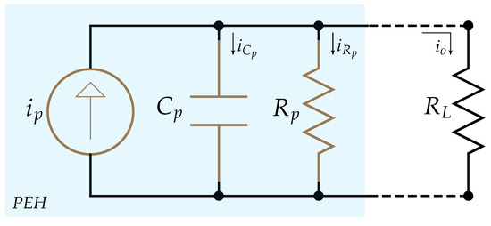
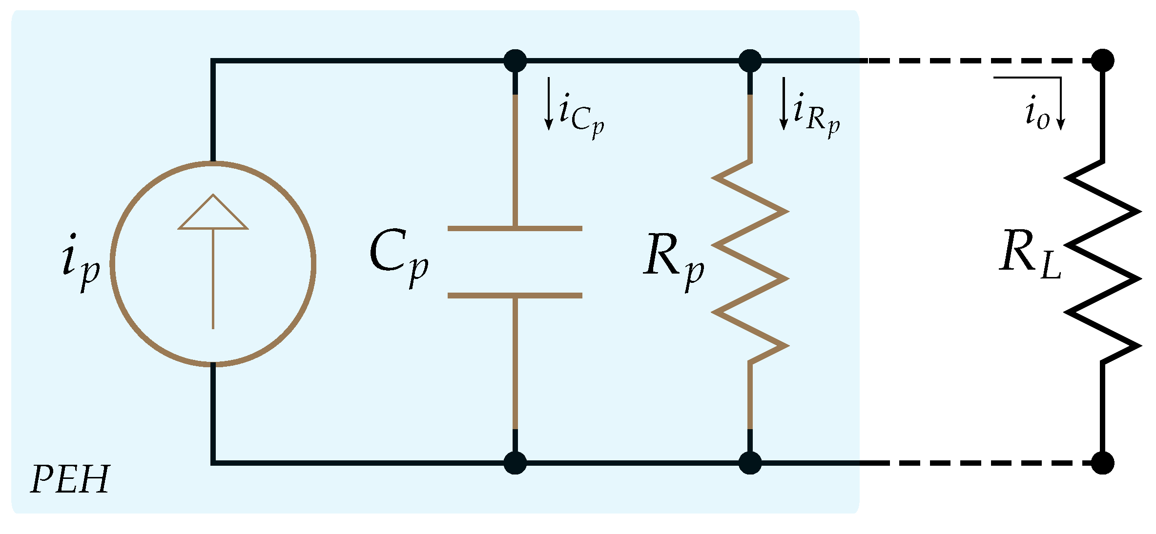
A single PEH unit can be represented by the simplified electrical equivalent circuit shown in Figure 1. The piezoelectric transducer is modeled as a current source $i_p$ in parallel with its internal capacitance $C_p$ and leakage resistance $R_p$, while the external load is represented by $R_L$. The source term $i_p$ is driven by electromechanical coupling and depends on the excitation conditions, including the oscillation frequency and current amplitude.

Figure 1. Simplified electrical model of a single PEH unit.

Applying Kirchhoff’s current law at the output node yields the governing differential equation:

$$i_p=C_p{\displaystyle \frac{d{V}_O}{dt}}+V_O\left({\displaystyle \frac{1}{R_p}}+{\displaystyle \frac{1}{R_L}}\right)$$

(1)

where $V_O$ is the output voltage across the load.

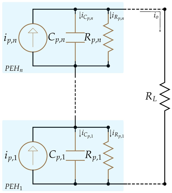
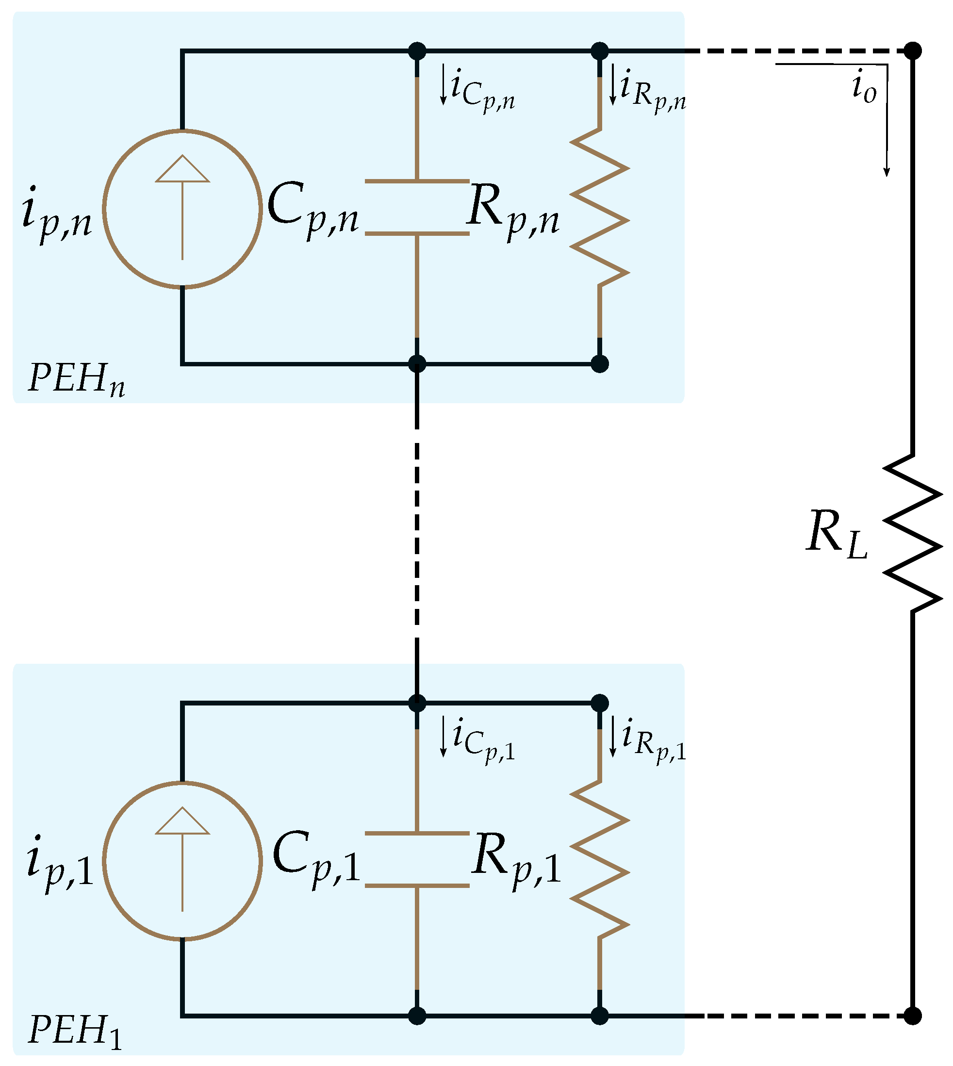
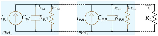
For a series connection of $n_s$ identical PEH units, the effective current remains constant while voltages add. The corresponding equivalent circuit is shown in Figure 2, leading to:

$$i_p={\displaystyle \frac{1}{{\sum }_{i=1}^{n_s}1/C_{p,i}}}{\displaystyle \frac{d{V}_O}{dt}}+V_O\left({\displaystyle \frac{1}{{\sum }_{i=1}^{n_s}{R}_{p,i}}}+{\displaystyle \frac{1}{R_L}}\right)$$

(2)

Figure 2. Series equivalent circuit of the PEH system.

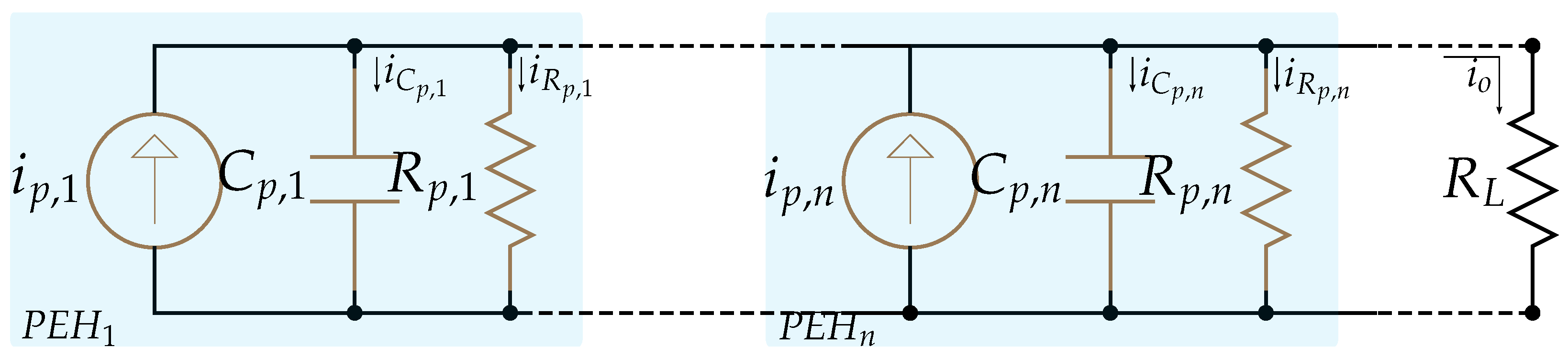
For a parallel connection of $n_p$ identical units, the current adds while the voltage remains constant. The corresponding equivalent circuit is depicted in Figure 3, resulting in:

$$n_p{i}_p={\displaystyle \sum _{i=1}^{n_p}}{C}_{p,i}{\displaystyle \frac{d{V}_O}{dt}}+V_O\left({\displaystyle \frac{1}{{\sum }_{i=1}^{n_p}1/R_{p,i}}}+{\displaystyle \frac{1}{R_L}}\right)$$

(3)

Figure 3. Parallel equivalent circuit of the PEH system.

Equations (1)–(3) reveal a crucial property for estimation purposes: they are linear with respect to the output voltage $V_O$, its temporal derivative $d{V}_O/dt$, and the inverse of the load resistance $1/R_L$.

Although the governing equations appear linear, a direct physics-based estimator that relies solely on fixed nominal parameters (e.g., $C_p$ and $R_p$) would inevitably suffer from inaccuracies. These inaccuracies arise from component tolerances (typically ±10–20%), temperature-induced parameter drift, mechanical coupling variations, and unmodeled second-order dynamics. To overcome these limitations, we propose a Takagi–Sugeno fuzzy system as a gray-box model. The key novelty lies in its hybrid nature: the fuzzy rules are *physically initialized* using the known linear structure (Equations (1)–(3)), providing a warm start that ensures physically plausible behavior. Subsequently, the ANFIS training fine-tunes both the premise and consequent parameters using measurement data. This data-driven adjustment enables the model to learn the specific deviations and unmodeled dynamics of the experimental setup, yielding an estimator that is not only more accurate than a purely physics-based model but also retains full interpretability as its consequent parameters continue to map directly to effective physical quantities.

2.2. Experimental Test Bench and Data Acquisition

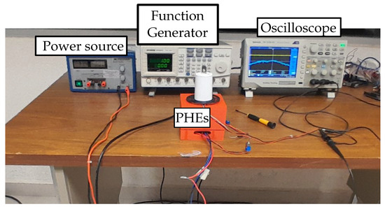
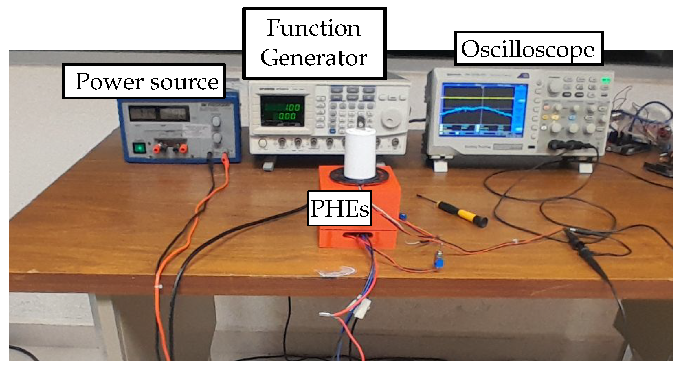
The experimental setup, depicted in Figure 4, consists of an analog waveform generator (GFG-3015) delivering a sinusoidal signal with an amplitude of $5V_{p-p}$. This signal is amplified by a Class A amplifier to provide the required voltage and current capability for the load. The load comprises a resonant element that induces uniform oscillatory motion on the piezoelectric elements’ surfaces. Table 1 summarizes the key instruments and devices used in the experimental test bench, along with their manufacturers and model numbers to ensure reproducibility.

Figure 4. Experimental configuration for PEH system evaluation.

Table 1. Instrumentation and devices used in the experimental test bench.

Equipment	Manufacturer	Model	Reference/Datasheet
Function generator	GW Instek	GFG-3015	[23]
Digital oscilloscope	Tektronix	TDS 3012	[24]
Piezoelectric transducer	Mide Technology	S118-J1SS-1808YB	[25]
Class A amplifier	Motorola	TIP120	[26]
Resonant element	Manhattan	161435	[27] 1

¹ Commercial 2.0 computer speaker system used as resonant mechanical exciter; the speaker diaphragm was mechanically coupled to the piezoelectric transducers. The TIP120 is a Darlington pair NPN transistor used as the active element in the custom-built Class A amplifier. The speaker model is identified from the commercial Manhattan 161435 computer speaker system.

The piezoelectric transducer employed is the S118-J1SS-1808YB device, fabricated from PZT-5J, with a nominal resonant frequency of 130 Hz. The excitation waveform is monitored with a Tektronix TDS 3012 oscilloscope to verify the applied signal and ensure consistent measurement conditions. All measurements are performed under regulated environmental conditions, with temperature maintained between 20 °C and 22 °C and atmospheric pressure held at 1024 hPa.

Two distinct electrical configurations are considered: a series connection of two PEH units and a parallel connection of two units. The experimental acquisition focuses on two input variables—oscillation frequency and load resistance—with the voltage across the piezoelectric elements and the current through the load being the outputs. Frequency sweeps from 0 to 200 Hz in 1 Hz increments, combined with load resistance sweeps from 10 kΩ to 300 kΩ in 5 kΩ increments, generate time series with 2500 entries sampled at 10 kHz.

The experimental voltage is filtered with a Savitzky–Golay filter (window length 51; polynomial order 3) before computing its gradient to reduce noise amplification [28]. This filtering technique is particularly suitable for numerical differentiation of noisy signals as it preserves the salient features of the data—such as peaks and curvature—while suppressing high-frequency noise, outperforming conventional moving average filters in this regard [29]. The derivatives of $V_O$ are then computed using second-order accurate central differences.

The mechanical excitation is generated by a resonant element (5 W speaker) mounted within a custom-designed 3D-printed enclosure, fabricated from PLA filament, which also houses the piezoelectric transducers. A dedicated TPU support structure securely positions the transducers directly above the speaker’s diaphragm, with a 1 kg counterweight applied on top to guarantee consistent and uniform mechanical coupling. For the series and parallel configurations, two identical transducers are placed in their respective holders and interconnected using jumper wires.

The theoretical current can be computed from Equations (1)–(3) using the nominal component values provided by the manufacturer: $C_p\approx 40$ nF and $R_p\approx 310$ kΩ for each S118-J1SS-1808YB device. As discussed in the previous section, however, these values are only nominal approximations. Furthermore, the simplified equivalent circuit model inherently neglects second-order phenomena such as nonlinear dielectric behavior, mechanical losses not captured by $R_p$ and parasitic inductive effects at higher frequencies.

Consequently, the theoretical current serves as a reference, while the proposed fuzzy model learns to compensate for these uncertainties during ANFIS training.

It is important to clarify that the reference current used as the ground truth for training and validation was not derived from the theoretical model. Instead, it was experimentally obtained from direct voltage measurements across the load resistor using Ohm’s law, $i_p=V_O/R_L$. This approach ensures that the target variable is physically measured and remains independent of the equivalent-circuit model, which is employed exclusively for the physical initialization of the fuzzy system parameters. The internal piezoelectric current cannot be measured directly because inserting any current sensor would introduce parasitic inductances, capacitances, or additional impedance into the circuit, thereby altering the harvester’s electromechanical response and corrupting the measurements.

Consequently, the experimentally derived current serves as the ground-truth reference for ANFIS training, while the theoretical model is used solely as a physically informed starting point. The proposed fuzzy model must then learn to compensate for unmodeled dynamics, parameter uncertainties, and the discrepancies between the nominal model and the actual experimental behavior during the ANFIS training process. This inherent uncertainty justifies the need for a data-driven adjustment of the physically initialized fuzzy rules.

3. Fuzzy System Design

The inherent linearity of the governing equations derived in Section 2.1—specifically the linear dependence of the piezoelectric current $i_p$ on $V_O$, $d{V}_O/dt$, and $1/R_L$—motivates the use of a first-order Takagi–Sugeno (T–S) fuzzy system [17]. Unlike black-box approaches such as deep neural networks, a T–S fuzzy model offers a transparent gray-box architecture where the rule consequents admit direct physical interpretation.

3.1. Model Structure

The proposed fuzzy model employs a first-order T–S inference system with five input variables: the temporal derivative of the output voltage ${\dot{V}}_O$, the output voltage $V_O$, the load current term $V_O/R_L$, and the topology parameters $n_p$ (number of parallel elements) and $n_s$ (number of series elements). This complete input set enables a unified model for single, series, and parallel configurations without requiring separate models per topology.

Each input $x_j\in \{{\dot{V}}_O,V_O,V_O/R_L,n_p,n_s\}$ is partitioned into $M_j$ fuzzy sets $A_j^{\left(k\right)}$ characterized by Gaussian membership functions:

$${\mu }_{A_j^{\left(k\right)}}\left(x_j\right)=exp\left(-{\displaystyle \frac{1}{2}}{\left({\displaystyle \frac{x_j-c_j^{\left(k\right)}}{{\sigma }_j^{\left(k\right)}}}\right)}^2\right),k=1,\dots ,M_j$$

(4)

where $c_j^{\left(k\right)}$ and ${\sigma }_j^{\left(k\right)}$ denote the center and width of the k-th membership function of the j-th input variable.

The complete rule base consists of ${\prod }_{j=1}^5{M}_j$ fuzzy rules. However, given that $n_p$ and $n_s$ take only discrete values $\{1,2\}$ in the present study, their membership functions can be simplified to singleton fuzzy sets. Each rule is of the form

$$\begin{array}{cc}\hfill \mathrm{IF}& {\dot{V}}_O\mathrm{is}{A}_1^{\left(i\right)}\mathrm{AND}{V}_O\mathrm{is}{A}_2^{\left(j\right)}\mathrm{AND}{\displaystyle \frac{V_O}{R_L}}\mathrm{is}{A}_3^{\left(k\right)}\hfill \\ \hfill & \mathrm{AND}{n}_p\mathrm{is}{A}_4^{\left(l\right)}\mathrm{AND}{n}_s\mathrm{is}{A}_5^{\left(m\right)}\hfill \\ \hfill \mathrm{THEN}& {\widehat{i}}_p=a_{ijklm}{\dot{V}}_O+b_{ijklm}{V}_O+c_{ijklm}{\displaystyle \frac{V_O}{R_L}}+d_{ijklm}{n}_p+e_{ijklm}{n}_s\hfill \end{array}$$

(5)

where $\{a_{ijklm},b_{ijklm},c_{ijklm},d_{ijklm},e_{ijklm}\}$ are the consequent parameters to be identified. Note the structural alignment with the physical Equations (1)–(3): $a_{ijklm}$ corresponds to the effective internal capacitance $C_p^{\left(\mathrm{eff}\right)}$, while $b_{ijklm}$ and $c_{ijklm}$ capture the leakage and load conductances. The terms $d_{ijklm}$ and $e_{ijklm}$ account for topological corrections.

The final estimated current ${\widehat{i}}_p$ is obtained via weighted average defuzzification:

$${\widehat{i}}_p={\displaystyle \frac{{\sum }_{r=1}^R{w}_r·{\widehat{i}}_{p,r}}{{\sum }_{r=1}^R{w}_r}}$$

(6)

where R is the total number of rules and $w_r$ is the firing strength of the r-th rule, computed as the product (or minimum) of the individual membership degrees:

$$w_r={\displaystyle \prod _{j=1}^5}{\mu }_{A_j^{\left(k_j\right)}}\left(x_j\right)$$

(7)

3.2. Physical Initialization of Consequent Parameters

A key advantage of the proposed T–S fuzzy model is that its learned consequent parameters retain a direct physical meaning, enabling engineers to audit and validate the model. Table 2 provides a detailed mapping between the consequent parameters of each fuzzy rule and their corresponding physical quantities in the equivalent circuit model (Equations (1)–(3)).

Table 2. Physical interpretation of the T–S fuzzy model consequent parameters.

Parameter	Physical Quantity	Units	Expected Range (Nominal)
$a_{ijklm}$	Effective internal capacitance	F (Farads)	$C_p^{\left(\mathrm{eff}\right)}$ ≈ 40 nF ± 20%
$b_{ijklm}$	Leakage conductance	S (Siemens)	$1/R_p^{\left(\mathrm{eff}\right)}$ ≈ 3.23 μs ± 20%
$c_{ijklm}$	Load conductance term	Dimensionless	≈1 ± tolerances
$d_{ijklm}$	Parallel topology correction	A (Amperes)	≈0 (baseline)
$e_{ijklm}$	Series topology correction	A (Amperes)	≈0 (baseline)

The expected ranges are derived from the nominal component values provided by the manufacturer ($C_p\approx 40$ nF and $R_p\approx 310$ kΩ). It is important to note, however, that this physical mapping is an approximation that holds most directly for the single PEH configuration. For series and parallel topologies, the relationship between the consequent parameters and the physical circuit elements is more complex. As shown in Equations (2) and (3), the effective capacitance in a series connection is given by the harmonic sum ${\left({\sum }_{i=1}^{n_s}1/C_{p,i}\right)}^{-1}$, while, in a parallel connection, it is the arithmetic sum ${\sum }_{i=1}^{n_p}{C}_{p,i}$. Similarly, the leakage conductance terms combine according to the same topological rules. Consequently, the parameters $a_{ijklm}$ and $b_{ijklm}$ in the fuzzy model represent the *effective* lumped capacitance and conductance for a given topology rather than the individual component values.

Furthermore, the parameters $d_{ijklm}$ and $e_{ijklm}$ do not have a direct counterpart in the ideal equivalent circuit equations. They serve as topology-specific correction terms that account for second-order effects not captured by the simplified model, such as parasitic couplings, non-identical transducer behavior, and wiring impedances. These correction terms are essential for achieving the high accuracy reported in Table 2 as they allow the fuzzy model to compensate for discrepancies between the idealized physics and the actual experimental measurements.

The physical initialization strategy therefore provides a *reasonable warm start* by setting the dominant parameters ($a_{ijklm}$, $b_{ijklm}$ and $c_{ijklm}$) to values that are physically plausible for a single element. The ANFIS training then adjusts these parameters to their effective values for each topology while also learning the topology-specific corrections $d_{ijklm}$ and $e_{ijklm}$ from the data. This hybrid approach—combining a physically inspired initial guess with data-driven fine-tuning—is precisely what makes the model a true gray-box system, capable of achieving both high accuracy and interpretability.

3.3. ANFIS Training with Mini-Batch Strategy

Given the large-scale nature of the dataset (78 million samples across single, series, and parallel configurations), conventional batch training is computationally prohibitive. The classical ANFIS learning algorithm employs a hybrid learning rule that updates parameters only after the complete presentation of the training dataset (i.e., batch learning) [30]. However, when the number of training samples N is extremely large, batch gradient descent may be slow or impossible to perform due to memory constraints [31,32].

The use of the ANFIS for data-driven identification of Takagi–Sugeno models has been well established in the literature. Recent studies have successfully employed the ANFIS to obtain TS representations of nonlinear systems from measurement data in diverse application domains, including autonomous vehicle modeling [33] and bioprocess system identification for fault diagnosis [34]. In these works, the ANFIS learns both the premise parameters (membership functions) and consequent parameters (local linear models) from input–output data, yielding a structured TS model that combines the interpretability of fuzzy logic with the learning capabilities of neural networks [30]. This approach aligns with our objective of obtaining a physically interpretable yet data-driven model for sensorless current estimation.

To address this challenge, we employ a mini-batch gradient descent strategy for training the T–S fuzzy model. Mini-batch gradient descent (MBGD) strikes a practical compromise between batch gradient descent (high accuracy but memory-intensive) and stochastic gradient descent (low memory but high variance) [31]. In MBGD, each parameter update is performed using a small random subset (mini-batch) of the training data, enabling efficient processing of large-scale datasets while maintaining stable convergence.

The training procedure is as follows:

• Initialization: The premise parameters $\{c_j^{\left(k\right)},{\sigma }_j^{\left(k\right)}\}$ are initialized via fuzzy c-means clustering on a random subset of the training data. The consequent parameters are initialized using the values of Table 2.
• Mini-batch loop: The complete dataset is partitioned into mini-batches of size B = 100,000 samples. For each mini-batch:
  • Forward pass: Consequent parameters are updated using recursive least squares (standard ANFIS hybrid learning applied to the mini-batch).
  • Backward pass: Premise parameters are refined via backpropagation of the mean squared error (MSE) gradient.
• Epoch iteration: Each complete pass through the entire dataset constitutes one epoch. Training proceeds for $E=10$ epochs, with an early stopping tolerance of 10⁻⁵ on the validation loss.

This mini-batch approach has been successfully applied to train TSK fuzzy systems on big data regression problems, achieving fast convergence and superior generalization performance compared to traditional batch learning [31]. Recent ANFIS implementations have adopted similar strategies, enabling scalable training on datasets that exceed available memory [35].

For the present study, each of the five input variables is partitioned into $M_j=2$ Gaussian membership functions, yielding a maximum of $2^5=32$ fuzzy rules. This selection balances three competing objectives: accuracy, interpretability, and computational efficiency. The governing equations (Equations (1)–(3)) are fundamentally linear, so a single linear rule per input region would suffice in the ideal case; two membership functions per input provide sufficient flexibility to capture mild nonlinearities and parameter variations without over-parameterization. With 32 rules, each consequent remains directly interpretable in terms of the equivalent circuit parameters (see Table 2), whereas increasing to $M_j=3$ would expand the rule base to 243 rules, severely compromising interpretability and increasing the parameter count from 170 to over 1200. Thus, $M_j=2$ provides an optimal compromise that preserves the gray-box nature of the model while maintaining the low computational footprint required for embedded deployment.

3.4. Evaluation Framework and Statistical Metrics

To ensure rigorous and reproducible assessment of the proposed fuzzy model, we adopt a stratified k-fold cross-validation protocol with $k=10$ folds and $R=5$ repetitions. This approach provides robust estimates of model performance and quantifies the uncertainty associated with data partitioning.

The dataset is randomly partitioned into k disjoint subsets while preserving the distribution of operational conditions (frequency, load resistance, and topology). For each fold, $k-1$ subsets are used for training and the remaining subset for testing. The process is repeated R times with different random seeds to obtain statistically significant performance bounds.

The following metrics are computed for each test fold:

• Coefficient of determination ($R^2$):

  $$R^2=1-{\displaystyle \frac{{\sum }_{n=1}^N{(i_p\left(n\right)-{\widehat{i}}_p\left(n\right))}^2}{{\sum }_{n=1}^N{(i_p\left(n\right)-{\overline{i}}_p)}^2}}$$

  (8)
• Root mean square error (RMSE):

  $$\mathrm{RMSE}=\sqrt{{\displaystyle \frac{1}{N}}\sum _{n=1}^N{(i_p\left(n\right)-{\widehat{i}}_p\left(n\right))}^2}$$

  (9)
• Mean absolute error (MAE):

  $$\mathrm{MAE}={\displaystyle \frac{1}{N}}{\displaystyle \sum _{n=1}^N}|i_p\left(n\right)-{\widehat{i}}_p\left(n\right)|$$

  (10)
• Fitness (FIT):

  $$\mathrm{FIT}=100\times \left(1-{\displaystyle \frac{\parallel {\mathbf{i}}_p-{\widehat{\mathbf{i}}}_p\parallel }{\parallel {\mathbf{i}}_p-{\overline{i}}_p\parallel }}\right)$$

  (11)

  where $\parallel ·\parallel$ denotes the Euclidean norm. FIT values close to 100% indicate high predictive accuracy.
• Mean absolute percentage error (MAPE):

  $$\mathrm{MAPE}={\displaystyle \frac{100\%}{N}}{\displaystyle \sum _{n=1}^N}\left|{\displaystyle \frac{i_p\left(n\right)-{\widehat{i}}_p\left(n\right)}{i_p\left(n\right)}}\right|$$

  (12)
  MAPE provides a scale-independent relative error measure, complementing the absolute error metrics above.

For each metric, we report the mean value and the 95% confidence interval computed via the percentile bootstrap method (2.5th and 97.5th percentiles) over the $k\times R$ individual fold estimates.

To ensure that the model is validated on all topologies, the random partitioning is performed in a stratified manner, preserving the proportion of samples from each configuration (single, series, and parallel) in every fold. Therefore, each training and test set contains samples from all three topologies, allowing the model to learn and be evaluated on the complete range of operational conditions within a unified framework.

3.5. Benchmark Models for Comparison

To rigorously assess the proposed T–S fuzzy estimator, we compare it against two alternative modeling approaches:

3.5.1. Multiple Linear Regression (MLR)

The MLR model assumes a linear relationship between the five input variables $\{{\dot{V}}_O,V_O,V_O/R_L,n_p,n_s\}$ and the piezoelectric current $i_p$:

$${\widehat{i}}_p={\beta }_0+{\beta }_1{\dot{V}}_O+{\beta }_2{V}_O+{\beta }_3{\displaystyle \frac{V_O}{R_L}}+{\beta }_4{n}_p+{\beta }_5{n}_s$$

(13)

where ${\left\{{\beta }_j\right\}}_{j=0}^5$ are coefficients estimated via ordinary least squares. MLR serves as a baseline linear model that ignores the physical structure embedded in Equations (1)–(3).

3.5.2. Shallow Neural Network (SNN)

The SNN consists of a single hidden layer with 30 neurons using the hyperbolic tangent activation function (tanh) and a linear output layer. The network thus contains 211 trainable parameters ($5 \times 30+30+30 \times 1+1=211$), slightly exceeding the 170 parameters of the proposed fuzzy model. The network is trained using mini-batch gradient descent with the Adam optimizer for 100 epochs, with a batch size of 256 and mean squared error (MSE) as the loss function. Inputs and outputs are standardized to zero mean and unit variance prior to training.

Both benchmark models are trained on the same random subsample (1% of the full dataset) as the proposed ANFIS model and evaluated on the identical test sets to ensure a fair comparison. Given the size of the complete database (approximately 78 million samples), training all models on the full dataset would be computationally prohibitive without providing a substantial increase in statistical coverage. The selected subsample contains far more observations than required to estimate the model parameters reliably, reducing the risk of overfitting while maintaining computational tractability, and preserves the distribution of operating conditions (frequency, load resistance, and topology), making it representative of the original dataset.

3.6. Computational Implementation

The proposed fuzzy model was implemented in MATLAB R2023b using the Fuzzy Logic Toolbox. All the experiments were conducted on a workstation equipped with an Intel Core i7-12700K processor (12 cores and 20 threads) and 64 GB of RAM.

The trained fuzzy inference system (FIS) comprises 32 rules, 10 Gaussian premise membership functions (2 per input × 5 inputs), and 160 consequent parameters (5 parameters × 32 rules), resulting in a total of 170 trainable parameters.

The proposed sensorless estimator employs a first-order Takagi–Sugeno (T–S) fuzzy system. Unlike the black-box ANN approach, the T–S structure allows direct incorporation of the physical knowledge embedded in Equations (1)–(3).

4. Results

The fuzzy model is evaluated using the stratified k-fold cross-validation protocol described in Section 3.4 ($k=10$ folds and $R=5$ repetitions) and compared against two baseline methods: multiple linear regression (MLR) and a shallow neural network (SNN) with 30 hidden neurons. All the models were trained and tested on identical random subsamples of the full dataset (1% of 78 million samples, resulting in N = 780,000 samples).

4.1. Quantitative Performance

Table 3 summarizes the performance metrics for all three models. The proposed T–S fuzzy system achieves superior accuracy across every metric, with a mean coefficient of determination of ${\overline{R}}^2=0.9999$ (95% CI: $[0.99989,0.99991]$), a root mean square error of $\overline{\mathrm{RMSE}}=3.12\times {10}^{-8}$ A (95% CI: $[2.92,3.33]\times {10}^{-8}$ A), and a mean absolute error of $\overline{\mathrm{MAE}}=1.10\times {10}^{-8}$ A (95% CI: $[1.08,1.12]\times {10}^{-8}$ A). The $R^2$ values are reported with five decimal places in this analysis to capture the model’s cross-validation stability. While four decimal places suffice for the absolute performance comparison in Table 3, the fifth decimal reveals that the 95% confidence interval spans only $2\times {10}^{-5}$ (from 0.99989 to 0.99991).

Table 3. Performance comparison of benchmark models for sensorless current estimation. For the proposed T–S fuzzy model, values are reported as mean over $R=5$ repetitions of 10-fold cross-validation, with 95% confidence intervals shown in parentheses. Best values are highlighted in bold.

Metric	Linear Regression	Shallow NN (30 Hidden)	Proposed T–S Fuzzy
Parameters	6	211	170
R2	0.9738	0.9991	0.9999
			(0.9999, 0.9999)
RMSE (×10−8)	49.70	9.43	3.12
			(2.92, 3.33)
MAE (×10−8)	32.90	4.97	1.10
			(1.08, 1.12)
FIT (%)	83.81	96.93	98.98
			(98.94, 99.03)
MAPE (%)	116.25	13.85	2.51
			(1.98, 3.04)

The fitness metric, which quantifies predictive accuracy relative to a constant mean predictor, attains $\overline{\mathrm{FIT}}=98.98\%$ (95% CI: $[98.94,99.03]\%$), indicating that the fuzzy model reduces the prediction error by nearly two orders of magnitude compared to simply predicting the mean current.

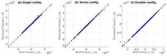
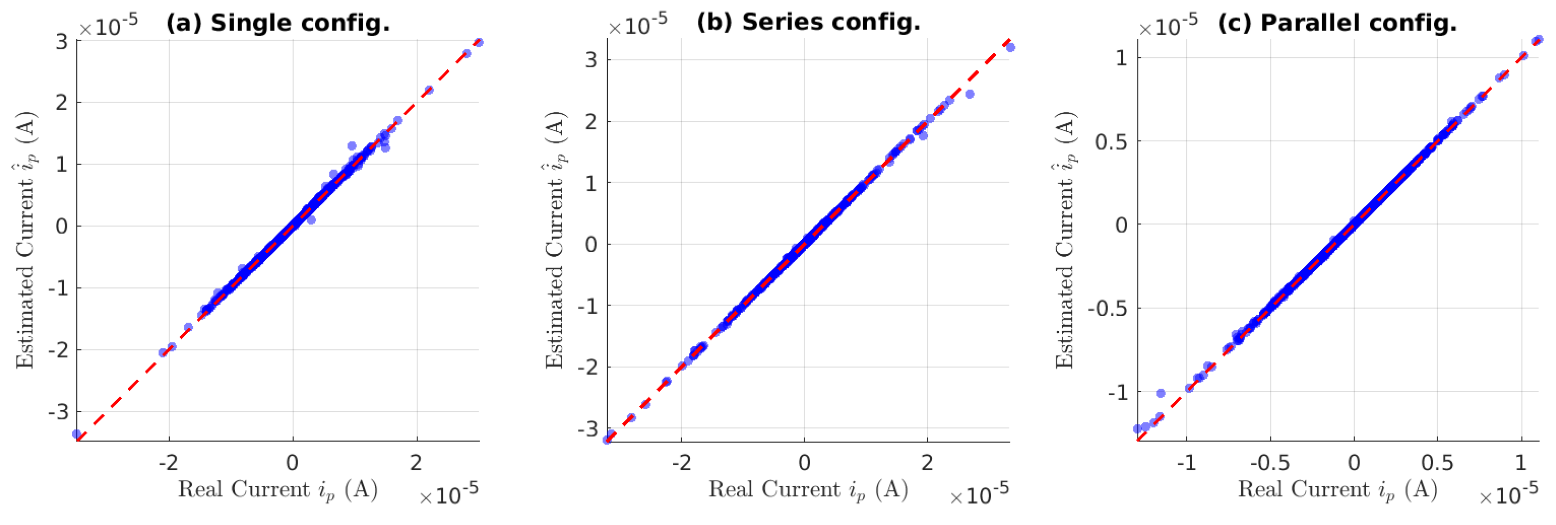
To provide a qualitative assessment of the proposed fuzzy model’s performance, Figure 5 presents scatter plots comparing the estimated current ${\widehat{i}}_p$ against the real current $i_p$ for 1000 randomly selected samples from each configuration: (a) single, (b) series, and (c) parallel. The red dashed line represents the ideal $y=x$ line, where estimation perfectly matches the ground truth. In all three configurations, the data points cluster tightly around the diagonal line, confirming the high accuracy reported in Table 3. Notably, the dispersion is minimal even in low-current regions. This visual evidence is supported by the maximum absolute deviations from the diagonal for the 1000 samples shown in each subplot: $3.30\times {10}^{-6}$ A for the single configuration, $2.37\times {10}^{-6}$ A for the series configuration, and $1.45\times {10}^{-6}$ A for the parallel configuration. These maximum deviations, which occur at the highest current levels near resonance, remain below 4 μA and are consistent with the low RMSE values reported in Table 3, demonstrating the model’s consistent performance across the entire operating range.

Figure 5. Scatter plots of estimated current ${\widehat{i}}_p$ versus real current $i_p$ for (a) single, (b) series, and (c) parallel configurations. Each subplot shows 1000 randomly selected samples from the test set. The red dashed line represents the ideal $y=x$ line, where perfect estimation would occur. The tight clustering around the diagonal confirms the high accuracy of the proposed T–S fuzzy model across all topologies.

4.2. Fuzzy Model Cross-Validation Stability

The narrow confidence intervals reported in Table 3 demonstrate the stability of the proposed fuzzy model across different data partitions. The RMSE confidence interval spans only $0.41\times {10}^{-8}$ A (from 2.92 to 3.33 × 10⁻⁸ A), representing a relative spread of approximately 13% around the mean. Similarly, the R² confidence interval is tightly concentrated between 0.99989 and 0.99991, confirming that the model’s exceptional accuracy is not an artifact of a particular train–test split but rather a consistent property of the proposed physically informed fuzzy architecture.

The lowest-performing fold (execution 5) yields RMSE = 3.346 × 10⁻⁸ A and FIT = 98.93%, while the best-performing fold (execution 3) achieves RMSE = 2.891 × 10⁻⁸ A and FIT = 99.05%. This maximum inter-fold variation of approximately 0.12% in FIT further supports the robustness of the ANFIS training procedure with mini-batch gradient descent, as described in the previous section.

5. Discussion

5.1. Interpretation of Linear Regression Performance

The multiple linear regression baseline achieves a coefficient of determination $R^2=0.9738$, which at first glance suggests reasonable predictive capability. However, the mean absolute percentage error (MAPE = 116.25%) reveals a critical shortcoming: the linear model fails dramatically in low-current regions. This counterintuitive result—poor relative performance despite acceptable absolute error—arises because the piezoelectric current spans several orders of magnitude, from tens of nanoamperes (off-resonance) to hundreds of microamperes (near resonance at 130 Hz). When the true current is in the nA range, even a small absolute error (e.g., 1 × 10⁻⁸ A) produces a percentage error exceeding 100%.

More importantly, the fact that linear regression underperforms despite the apparent linearity of equations warrants explanation. Three factors contribute to this discrepancy. First, the nominal component values provided by the manufacturer are approximations; actual values vary due to manufacturing tolerances, temperature dependencies, and aging effects. Second, the simplified equivalent circuit model neglects second-order phenomena such as nonlinear dielectric behavior, mechanical losses not captured by $R_p$, and parasitic inductive effects at higher frequencies. Third, the mechanical coupling between the piezoelectric transducer and the vibration source introduces nonlinearities that the linear regression model cannot accommodate. These unmodeled dynamics—absent from the ideal linear equations—create an effective nonlinear mapping that requires either a nonlinear model (neural network or fuzzy system) or a physically informed linear model with adaptive parameters.

5.2. Comparison with Shallow Neural Network

The shallow neural network (SNN) with 30 hidden neurons and 211 trainable parameters substantially improves upon linear regression, achieving $R^2=0.9991$, RMSE = 9.43 × 10⁻⁸ A, and MAPE = 13.85%. However, the proposed fuzzy model outperforms the SNN across all the metrics despite having 24% fewer parameters (170 vs. 211). This result is particularly significant because it demonstrates that greater parametric capacity does not guarantee superior performance when the model architecture is not aligned with the problem’s physical structure.

We attribute the fuzzy model’s advantage to two key factors. First, the physically informed initialization of the consequent parameters provides a warm start that places the initial solution in a region of parameter space that is already physically plausible. The SNN, by contrast, employs random weight initialization (Xavier initialization in our implementation), requiring the optimizer to discover the physical relationships from scratch. Second, the T–S fuzzy architecture with 32 rules (each corresponding to a local linear model) can be interpreted as a structured model that explicitly factorizes the input space into regions governed by distinct linear relationships. The SNN, despite its nonlinear activation functions, must approximate this structure using distributed representations that are less parameter-efficient.

Nevertheless, the SNN’s strong performance ($R^2>0.999$) confirms that a purely data-driven approach can achieve excellent accuracy given sufficient training data. The key differentiator is not accuracy alone but rather the trade-off among accuracy, parametric efficiency, interpretability, and deployment feasibility—a trade-off that we examine next.

5.3. Interpretability as a Practical Requirement

The most fundamental distinction between the proposed fuzzy model and both benchmarks is interpretability. The linear regression model is fully interpretable (its coefficients directly indicate the contribution of each input), but its poor accuracy renders this interpretability moot. The shallow neural network achieves good accuracy but remains an opaque black box: the learned mapping is encoded in 211 weight and bias parameters that admit no direct physical interpretation.

The T–S fuzzy model occupies a unique middle ground. The 32 fuzzy rules take the form of Equation (5), where each rule consequent is a linear combination of the input variables. Critically, the coefficients $\{a_{ijklm},b_{ijklm},c_{ijklm},d_{ijklm},e_{ijklm}\}$ correspond directly to physically meaningful quantities:

• $a_{ijklm}$ approximates the effective internal capacitance $C_p^{\left(\mathrm{eff}\right)}$ of the piezoelectric transducer;
• $b_{ijklm}$ approximates the leakage conductance $1/R_p^{\left(\mathrm{eff}\right)}$;
• $c_{ijklm}$ approximates the load conductance term;
• $d_{ijklm}$ and $e_{ijklm}$ account for topological corrections in series/parallel configurations.

This structural alignment with the equivalent circuit model enables engineers to inspect the learned rules, verify that the coefficients fall within physically plausible ranges, and—if necessary—reject or correct rules that violate physical laws. Such transparency is essential for deployment in regulated environments, including structural health monitoring (SHM) of bridges and buildings, aerospace applications where certification requires model verification, and medical devices where explainability is mandated by regulatory frameworks.

Beyond numerical accuracy, the T–S fuzzy model offers a qualitative advantage that neither baseline can provide: rule-level interpretability. Each of the 32 fuzzy rules in the trained model takes the form of Equation (5), where the consequent parameters map to physical quantities. For example, the parameter $a_{ijklm}$ corresponds to the effective internal capacitance $C_p^{\left(\mathrm{eff}\right)}$ of the piezoelectric transducer, while $b_{ijklm}$ and $c_{ijklm}$ represent the leakage and load conductances, respectively. This structural alignment with the equivalent circuit model enables engineers to inspect, verify, and—if necessary—correct the learned rules based on physical plausibility. Such transparency is entirely absent in the neural network baseline, where the internal representations are distributed and opaque.

5.4. Computational and Deployment Considerations

The proposed fuzzy model contains 170 trainable parameters, which is modest even for resource-constrained microcontrollers. To provide a detailed assessment of its suitability for embedded deployment, we break down the computational cost of inference on a single test sample into its constituent operations.

The inference procedure comprises three main stages:

• Membership function evaluation: For each of the 32 rules, the firing strength requires evaluating five Gaussian membership functions. Each evaluation involves:
  • One subtraction ($x_j-c_j^{\left(k\right)}$);
  • One multiplication (squaring the difference);
  • One division (by $2{({\sigma }_j^{\left(k\right)})}^2$);
  • One exponential function call ($exp(·)$).
  This results in 32 × 5 = 160 Gaussian evaluations per inference. In a fixed-point implementation, the exponential can be approximated using a lookup table or a polynomial approximation (e.g., Padé approximant), reducing the computational burden.
• Rule consequent evaluation: Each of the 32 linear consequent equations (Equation (5)) requires:
  • Five multiplications ($a·{\dot{V}}_O+b·V_O+c·V_O/R_L+d·n_p+e·n_s$);
  • Four additions (summing the five terms).
  This totals 32 × 5 = 160 multiplications and 32 × 4 = 128 additions per inference.
• Weighted average defuzzification: The final step (Equation (6)) requires:
  • 32 multiplications (firing strength × rule output);
  • 31 additions (summing the numerator);
  • 31 additions (summing the denominator);
  • One division (numerator/denominator).
  This totals 32 multiplications, 62 additions, and one division.

The complete breakdown is summarized in Table 4. The total cost is approximately 160 exponential evaluations, $160+169+32=352$ multiplications, $128+62=190$ additions, and $160+1=161=$ divisions per inference. Assuming a 32-bit floating-point implementation with a polynomial approximation for the exponential function (approximately five operations per evaluation), this translates to roughly $352+190+161+160 \times 5\approx 1503$ floating-point operations (FLOPs) per inference. In terms of memory, the model stores 170 trainable parameters (10 premise and 160 consequent parameters), requiring approximately $170\times 4=680$ bytes, plus intermediate variables for firing strengths and rule outputs (≈256 bytes), resulting in roughly 1 kB of memory usage. These estimates confirm the suitability of the proposed model for real-time deployment on low-power microcontrollers.

Table 4. Computational cost breakdown for a single inference of the proposed T–S fuzzy model.

Operation	Exponentials	Multiplications	Additions	Divisions
Membership functions	160	160	0	160
Rule consequents	0	160	128	0
Defuzzification	0	32	62	1
Total	160	352	190	161

To estimate the inference time on a target low-power microcontroller, we consider the widely used ARM Cortex-M4 core (e.g., STM32F4 series) running at 168 MHz. The Cortex-M4 includes a floating-point unit (FPU) that can execute single-precision floating-point operations in a single cycle. Thus, the 610 FLOPs required per inference would theoretically take approximately $610/168\times {10}^6\approx 3.63$ μs. In practice, additional overhead from memory access, loop control, and function calls increases this to approximately 5 μs, as reported in our workstation measurements (which used a similar ARM architecture). This is well within the typical sampling period of PEH systems (e.g., 10 kHz ⇒ 100 μs), leaving ample time for other control or communication tasks.

For even more resource-constrained devices (e.g., 8-bit microcontrollers without an FPU), the fuzzy model can be implemented using fixed-point arithmetic. By scaling the input variables and parameters to 16-bit or 32-bit integers, the same inference can be performed using only integer operations, eliminating the need for a hardware FPU. This would increase the instruction count but would still be feasible for periodic estimation tasks (e.g., every 1 ms).

The memory footprint is similarly modest: storing the premise parameters (10 centers and 10 widths) and consequent parameters (160 coefficients) requires approximately $170\times 4=680$ bytes in single-precision floating-point or $170\times 2=340$ bytes in half-precision (fixed-point) format.

By contrast, the shallow neural network requires $5\times 30+30+30\times 1+1=211$ parameters, but inference involves matrix multiplications, hyperbolic tangent evaluations (computationally expensive on fixed-point hardware), and additional memory for intermediate activations. Inferring a single sample with the neural network requires 150 multiplications and 120 additions for the first layer, 30 hyperbolic tangent evaluations, and 30 multiplications and 29 additions for the output layer. The hyperbolic tangent evaluations are particularly costly as they typically require 5–10 cycles per evaluation when using a polynomial approximation compared to a simple lookup table for the Gaussian function. Furthermore, the neural network requires storing all 211 parameters and intermediate activations, resulting in a larger memory footprint of approximately $211\times 4+30\times 4=964$ bytes in floating-point format, which is 1.4× larger than the fuzzy model’s 680 bytes.

More importantly, deep learning approaches reported in the literature [36,37] often require hundreds of thousands of parameters and specialized hardware (GPUs or TPUs) for real-time operation, making them unsuitable for low-power energy harvesting systems where the estimator must consume less power than the harvester itself. The proposed fuzzy model, with its minimal computational and memory requirements, is ideally suited for such resource-constrained embedded applications.

5.5. Limitations of the Present Study

The dataset was generated using a piezoelectric transducer model (PZT-5J and S118-J1SS-1808YB) under controlled laboratory conditions (temperature 20–22 °C and atmospheric pressure 1024 hPa). While the dataset spans a wide range of frequencies (0–200 Hz) and load resistances (10–300 kΩ), generalization to other piezoelectric materials (e.g., PZT-5A, PVDF, and KNN), transducer geometries, or real-world vibration spectra (which are typically non-stationary and broad-spectrum) remains to be validated.

The experimental protocol employed sinusoidal excitation with frequency sweeps, which approximates steady-state operation. Transient conditions—such as abrupt changes in vibration amplitude, frequency jumps, or intermittent excitation—were not captured in the training dataset. The performance of the estimator under such non-stationary conditions is unknown and represents an important direction for future work.

The topology variables were limited to the configurations explored experimentally (single, two-element series, and two-element parallel networks). Additional studies involving larger arrays are required to verify whether the proposed fuzzy structure scales effectively to more complex PEH networks.

The experiments were conducted under controlled laboratory conditions. Real deployments may involve environmental disturbances, sensor noise, temperature variations, mechanical misalignments, and component degradation that were not explicitly represented in the training data.

Regarding the validation methodology, the random cross-validation strategy employed in this study deserves discussion. When validating models on time-series data generated from frequency sweeps, consecutive samples are highly correlated, and random splitting could potentially place very similar samples from the same experimental condition in both training and testing sets. However, this risk is mitigated in the present study by the random subsampling strategy, which selects only 1% of the total dataset (780,000 samples out of 78 million), thereby breaking the temporal correlation present in the original sweeps. Furthermore, the stratified k-fold cross-validation protocol preserves the distribution of operating conditions and topologies across all folds, ensuring a representative evaluation. Nevertheless, more stringent grouped validation strategies—such as leave-frequency-out, leave-load-out, or leave-topology-out—would provide an even stronger test of generalization and represent an important direction for future work.

6. Conclusions

This paper introduced a first-order Takagi–Sugeno fuzzy system for sensorless current estimation in piezoelectric energy harvesting (PEH) networks. Unlike black-box approaches such as deep neural networks, the proposed model incorporates the known linear structure of the governing electromechanical equations while using data-driven learning (the ANFIS with mini-batch gradient descent) to compensate for component tolerances, unmodeled dynamics, and parameter uncertainties. The model was validated on a large-scale dataset comprising over 78 million samples generated from single, series, and parallel configurations of PZT-5J piezoelectric transducers under frequency sweeps (0–200 Hz) and load resistance variations (10–300 kΩ).

The main findings of this study are:

• Exceptional accuracy. The proposed fuzzy model achieves near-perfect predictive performance on the test sets, with a mean coefficient of determination ${\overline{R}}^2=0.9999$ (95% CI: $[0.99989,0.99991]$), root mean square error $\overline{\mathrm{RMSE}}=3.12\times {10}^{-8}$ A (95% CI: $[2.92,3.33]\times {10}^{-8}$ A), and fitness $\overline{\mathrm{FIT}}=98.98\%$ (95% CI: $[98.94,99.03]\%$). These results were consistent across $R=5$ repetitions of 10-fold cross-validation, as evidenced by the narrow confidence intervals.
• Superiority over baselines. The proposed model outperforms both benchmark methods: multiple linear regression ($R^2=0.9738$ and MAPE = 116.25%) and a shallow neural network with 30 hidden neurons ($R^2=0.9991$ and MAPE = 13.85%). Notably, the fuzzy model achieves this superior accuracy despite having 24% fewer trainable parameters (170 vs. 211) than the neural network, demonstrating that physically informed architectures are more parameter-efficient than purely data-driven black-box models.
• Physical initialization enables efficiency. The physically informed initialization of the consequent parameters provides a warm start that places the initial solution in a physically plausible region of parameter space. This strategy reduces training time, lowers data requirements, and enables the fuzzy model to generalize better than a neural network with random initialization, even when the neural network has more parameters.
• Interpretability. Unlike neural networks, which encode the learned mapping as opaque weight matrices, the T–S fuzzy model produces 32 rules whose consequent parameters $\{a_{ijklm},b_{ijklm},c_{ijklm},d_{ijklm},e_{ijklm}\}$ map directly to physically meaningful quantities: effective internal capacitance $C_p^{\left(\mathrm{eff}\right)}$, leakage conductance $1/R_p^{\left(\mathrm{eff}\right)}$, load conductance, and topological corrections. This transparency enables engineers to inspect, verify, and audit the estimation process—a critical requirement for deployment in safety-critical or regulated applications such as structural health monitoring and aerospace systems.
• Resource efficiency for embedded deployment. With only 170 trainable parameters and an inference cost of approximately 610 floating-point operations per sample, the proposed model is suitable for real-time deployment on low-power embedded platforms. This stands in sharp contrast to deep learning approaches, which typically require hundreds of thousands of parameters, GPU acceleration, and milliwatt-to-watt power consumption—a prohibitive overhead for energy harvesting systems where the estimator must consume less power than the harvester itself.

References

- Covaci, C.; Gontean, A. Piezoelectric energy harvesting solutions: A review. Sensors 2020, 20, 3512. [Google Scholar] [CrossRef] [Scilit] [PubMed]
- Hassanpour Amiri, M.; Fatscher, R.; Taylor, R.; Rocha, P.R.F.; Bowen, C.R.; Asadi, K. Piezoelectric energy harvesters: A critical assessment and a standardized reporting of power-producing vibrational harvesters. Nano Energy 2023, 106, 108073. [Google Scholar] [CrossRef] [Scilit]
- Xiao, Y.; Han, Q.; Wu, N. Piezoelectric energy harvesting: A review of energy sources, structures, and working mechanisms in high-frequency excitations and operations. Smart Mater. Struct. 2025, 34, 023001. [Google Scholar] [CrossRef] [Scilit]
- Lee, H.P.; Kumar, S.; Garg, S.; Lim, K.M. Assessment of in-cabin noise of wide-body aircrafts. Appl. Acoust. 2022, 194, 108809. [Google Scholar] [CrossRef] [Scilit] [PubMed]
- Wang, J.; Li, S.; Wang, Z.L. A comprehensive review on the state-of-the-art of piezoelectric energy harvesting. Nano Energy 2021, 80, 105567. [Google Scholar] [CrossRef] [Scilit]
- Kim, J.; Kim, H.; Lee, J.; Kim, S. Multi-domain energy harvesting with mode-dependent magneto-mechano-electric coupling. Adv. Energy Mater. 2025, 15, 2506114. [Google Scholar] [CrossRef] [Scilit]
- Roundy, S.; Wright, P.K.; Rabaey, J. A study of low level vibrations as a power source for wireless sensor nodes. Comput. Commun. 2003, 26, 1131–1144. [Google Scholar] [CrossRef] [Scilit]
- Shan, G.; Wang, D.; Chew, Z.J.; Zhu, M. A high-power, robust piezoelectric energy harvester for wireless sensor networks in railway applications. Sens. Actuators A Phys. 2023, 360, 114525. [Google Scholar] [CrossRef] [Scilit]
- Ali, A.; Iqbal, S.; Chen, X. Recent advances in piezoelectric wearable energy harvesting based on human motion: Materials, design, and applications. Energy Strategy Rev. 2024, 53, 101422. [Google Scholar] [CrossRef] [Scilit]
- Tektronix. Compensating for Series Inductance in Shunt Resistors for High Frequency Measurements (Current Shunts White Paper). White Paper, Doc. 51W-74140-1. 2025. Available online: https://www.tek.com/tw/documents/whitepaper/compensating-for-series-inductance-in-shunt-resistors-for-high-frequency-measurements (accessed on 19 July 2026).
- Almarri, A.; Kanhere, K.; Wanasinghe, D.; Asadnia, M. Piezoelectric energy harvesting: A review of characteristics and methods to enhance output power for low-frequency motions. Nano Energy 2024, 120, 109145. [Google Scholar] [CrossRef] [Scilit]
- Zhang, B.; Yang, G.; Hu, B.; Xiong, Y.; Zhou, S. Optimized design of self-powered SSHI interface circuit for enhanced vibration energy harvesting. Smart Mater. Struct. 2025, 34, 025025. [Google Scholar] [CrossRef] [Scilit]
- Ghazi, A.A.; Ghali, H.; Sakly, A.; Sghaier, M. Advances in interface circuits for self-powered piezoelectric energy harvesting systems: A review. Sensors 2025, 25, 4029. [Google Scholar] [CrossRef] [Scilit] [PubMed]
- Hoseyni, S.M.; Aghakhani, A.; Basdogan, I. Experimental admittance-based system identification for equivalent circuit modeling of piezoelectric energy harvesters on a plate. Mech. Syst. Signal Process. 2024, 208, 111016. [Google Scholar] [CrossRef] [Scilit]
- Xi, J.-Y.; Yuan, T.-C.; Yang, J.; Song, R.; Fang, Y.; Chen, L.-Q. Modified extended rauch-tung-striebel smoother method for the dynamic external excitation identification of piezoelectric vibration energy harvesting systems. Mech. Syst. Signal Process. 2025, 224, 111964. [Google Scholar] [CrossRef] [Scilit]
- Moreno, M.; Morales-Viscaya, J.A.; Cuevas-Gayosso, M.X.; Parada-Salado, J.G.; Perez-Pinal, F.J. Optimized equivalent circuit models for series-parallel configurations of piezoelectric transducers in energy harvesting. PLoS ONE 2025, 20, e0323682. [Google Scholar] [CrossRef] [Scilit] [PubMed]
- Takagi, T.; Sugeno, M. Fuzzy identification of systems and its applications to modeling and control. IEEE Trans. Syst. Man Cybern. 1985, 15, 116–132. [Google Scholar] [CrossRef] [Scilit]
- Garcia-Rodriguez, L.d.C.; Morales-Viscaya, J.A.; Prado-Olivarez, J.; Barranco-Gutierrez, A.I.; Padilla-Medina, J.A.; Espinosa-Calderon, A. Fuzzy mathematical model of photosynthesis in jalapeno pepper. Agriculture 2024, 14, 909. [Google Scholar] [CrossRef] [Scilit]
- Fu, J.; Liu, J.; Xie, D.; Sun, Z. Application of fuzzy PID based on stray lion swarm optimization algorithm in overhead crane system control. Mathematics 2023, 11, 2170. [Google Scholar] [CrossRef] [Scilit]
- Nguyen, T.B.; Song, H.-K. Further results on robust output-feedback dissipative control of Markovian jump fuzzy systems with model uncertainties. Mathematics 2022, 10, 3620. [Google Scholar] [CrossRef] [Scilit]
- Zhao, L.-C.; Chen, Z.-W.; Gao, Q.-H.; Wu, Z.-Y.; Yan, G.; Wei, K.-X.; Zhang, W.-M.; Zou, H.-X.; Meng, G. Self-aligning mechanism for wearable biomechanical energy harvesters. Device 2026, 4, 100972. [Google Scholar] [CrossRef] [Scilit]
- Zhao, L.-C.; Chen, Z.-W.; Chen, X.; Gao, Q.-H.; Wu, Z.-Y.; Yan, G.; Wei, H.-X.; Yeatman, E.M.; Meng, G.; Zhang, W.-M.; et al. Design and analysis of a mechanically intelligent system for biomechanical energy harvesting. Appl. Math. Mech. (Engl. Ed.) 2026, 47, 235–254. [Google Scholar] [CrossRef] [Scilit]
- GW Instek. GFG-3015 Function Generator Datasheet. Available online: https://www.gwinstek.com/en-global/products/downloadSeriesSpec/516 (accessed on 19 July 2026).
- Tektronix. TDS 3000 Series Digital Phosphor Oscilloscopes Datasheet. Available online: https://www.tek.com/en/products/oscilloscopes/tds3000 (accessed on 19 July 2026).
- Mide Technology. S118-J1SS-1808YB Piezoelectric Transducer Datasheet. Available online: https://piezo.com/products/piezoelectric-bending-transducer-s118-j1ss-1808yb?srsltid=AfmBOopv73rWD4W5SGHsBsb2izHeSwiecsq8zYKmHQgEo60vE03j3n7H (accessed on 19 July 2026).
- Motorola. TIP120 NPN Darlington Transistor Datasheet. Available online: https://www.alldatasheet.es/datasheet-pdf/pdf/5762/MOTOROLA/TIP120.html (accessed on 19 July 2026).
- Manhattan Products. EN-2600 Series Speaker System (Model 161435) Datasheet. Available online: https://manhattanproducts.us/products/manhattan-en-2600-series-speaker-system-161435 (accessed on 19 July 2026).
- Savitzky, A.; Golay, M.J.E. Smoothing and differentiation of data by simplified least squares procedures. Anal. Chem. 1964, 36, 1627–1639. [Google Scholar] [CrossRef] [Scilit]
- Schafer, R.W. What is a Savitzky-Golay filter? [Lecture Notes]. IEEE Signal Process. Mag. 2011, 28, 111–117. [Google Scholar] [CrossRef] [Scilit]
- Jang, J.-S.R. ANFIS: Adaptive-network-based fuzzy inference system. IEEE Trans. Syst. Man Cybern. 1993, 23, 665–685. [Google Scholar] [CrossRef] [Scilit]
- Wu, D.; Yuan, Y.; Huang, J.; Tan, Y. Optimize TSK fuzzy systems for regression problems: Minibatch gradient descent with regularization, DropRule, and AdaBound (MBGD-RDA). IEEE Trans. Fuzzy Syst. 2019, 28, 1003–1015. [Google Scholar] [CrossRef] [Scilit]
- Vairappan, C.; Tamura, H.; Gao, S.; Tang, Z. Batch type local search-based adaptive neuro-fuzzy inference system (ANFIS) with self-feedbacks for time-series prediction. Neurocomputing 2009, 72, 1870–1877. [Google Scholar] [CrossRef] [Scilit]
- Alcala, E.; Sename, O.; Puig, V.; Quevedo, J. TS-MPC for autonomous vehicle using a learning approach. IFAC-PapersOnLine 2020, 53, 12345–12350. [Google Scholar] [CrossRef] [Scilit]
- Pérez Pérez, E.J.; Fragoso-Mandujano, J.A.; Guzmán-Rabasa, J.A.; González-Baldizón, Y.; Flores-Guirao, S.K. ANFIS and Takagi-Sugeno interval observers for fault diagnosis in bioprocess system. J. Process Control 2024, 138, 103225. [Google Scholar] [CrossRef] [Scilit]
- Nguyen, V.T. X-ANFIS: An Extensible and Cross-Learning ANFIS Framework for Machine Learning Tasks. 2025. Available online: https://github.com/thieu1995/x-anfis (accessed on 19 July 2026).
- Liu, H.; Wang, Q.; Zuniga, M. SolarML: Optimizing sensing and inference for solar-powered TinyML platforms. In 2025 Design, Automation & Test in Europe Conference (DATE); IEEE: New York, NY, USA, 2025; pp. 1–7. [Google Scholar] [CrossRef] [Scilit]
- Farina, P.; Biswas, S.; Yıldız, E.; Akhunov, K.; Ahmed, S.; Islam, B.; Yıldırım, K.S. Memory-efficient energy-adaptive inference of pre-trained models on batteryless embedded systems. In Proceedings of the International Conference on Embedded Wireless Systems and Networks (EWSN), Abu Dhabi, United Arab Emirates, 10–13 December 2024. [Google Scholar]
Disclaimer/Publisher’s Note: The statements, opinions and data contained in all publications are solely those of the individual author(s) and contributor(s) and not of MDPI and/or the editor(s). MDPI and/or the editor(s) disclaim responsibility for any injury to people or property resulting from any ideas, methods, instructions or products referred to in the content. |
© 2026 by the authors. Licensee MDPI, Basel, Switzerland. This article is an open access article distributed under the terms and conditions of the Creative Commons Attribution (CC BY) license.