


Abstract
This paper presents a low-power fully integrated sine signal generator for on-chip bioimpedance spectroscopy applications. The circuit is based on a relaxation oscillator, which generates a triangular signal, followed by a sixth-order Gm-C bandpass filter (BPF) that linearizes the waveform. Both blocks, designed in a 0.18 m CMOS process with 1.8 V supply, make use of a current division technique to generate low-frequency signals without requiring high-valued passive components. The relaxation oscillator features an extended frequency tuning range from 300 Hz to 300 kHz, controlled via a tuning current and a digital capacitor bank. The sine output waveform spans from 1 kHz to 50 kHz, and exhibits a −48.8 dB total harmonic distortion at 10 kHz with 18 mV amplitude. The overall system area is 0.7 and the power consumption is lower than 30 W.
1. Introduction
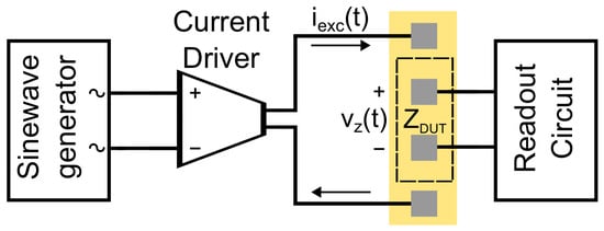
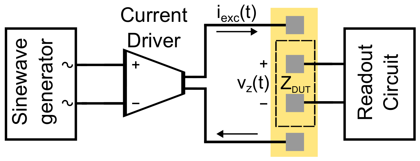
Bioimpedance spectroscopy (BIS) is a noninvasive, cost-effective, and versatile technique in biomedical applications, such as body composition estimation, tissue characterization, and early lymphedema detection, among others [1,2,3,4,5,6,7,8], which relies on acquiring the bioimpedance (BioZ) spectrum by sweeping the excitation signal across a range of frequencies. In order to foster major advancements in portable point-of-care (POC) devices, there is a growing demand for high-performance, compact, and energy-efficient integrated circuit solutions capable of driving precise BIS instrumentation. While wide-band signal excitation offers faster measurement times by simultaneously characterizing multiple frequencies, single-tone excitation provides a higher signal-to-noise ratio and better measurement sensitivity [9,10,11], which are critical specifications for these applications. Figure 1 illustrates the block diagram of a BioZ measurement front-end. The sine-wave generator serves as a precise voltage reference and drives a dedicated, high-input-impedance current driver (e.g., a V-I converter), which injects the excitation current into the target biological tissue (). The resulting voltage response is acquired by the readout stage. The sine-wave generator operates under light loading conditions, ensuring low distortion, a well-defined operating frequency, and the tunability range required by the application, while the current driver maintains operation strictly within safety bounds for biomedical sensing.
Figure 1.
Block diagram of a BioZ measurement front-end.
This work focuses exclusively on the sine-wave generator block, which can be either digitally implemented or based on analog oscillator topologies. Digital architectures, such as Direct Digital Synthesis (DDS) and generators based on Digital-to-Analog Converters (DACs), are highly linear. However, they rely on high-speed clocks and high-resolution DACs, which may result in high power and silicon area consumption [11,12,13]. In order to achieve low-power sine-wave generation, the Wien-bridge oscillator is often used in the literature [14,15,16], but it requires an automatic gain control circuit to reduce the third-harmonic, and digitally programmable resistors in the feedback network for frequency tuning. Furthermore, as the feedback resistors must be matched to prevent frequency instability, multiple resistor banks are needed, significantly increasing the area of the circuit [16]. Finally, large-sized passive components are required to generate low-frequency signals, which in some cases leads to the use of off-chip components [15]. Alternatively, Gm-C sinusoidal generators avoid the area overhead of integrated resistors, but their inherent linearity is limited [17]. As for sine synthesizers based on wave-shaping techniques, they rely on the non-linear characteristics of transistors in the sub-threshold region to generate the sine wave, resulting in high harmonic distortion due to their strong dependence on bias conditions [18].
This paper presents a tunable sine waveform generator based on a relaxation oscillator and a sixth-order Gm-C bandpass filter. A current division technique is applied to both subcircuits in order to achieve low-frequency operation without requiring high-value passive components. Additionally, multiple frequency control mechanisms are incorporated to extend the achievable operating frequency range while preserving low-power operation. The remainder of the paper is organized as follows: Section 2 describes the design and characteristics of the proposed tunable relaxation oscillator, and Section 3 presents the design of the sixth-order Gm-C bandpass filter, based on low-Gm operational transconductance amplifiers (OTAs). Section 4 shows the post-layout simulation results of the proposed sine waveform generator and compares the design with related works in the literature. Finally, the main conclusions are summarized in Section 5.
2. Relaxation Oscillator
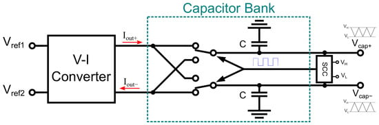
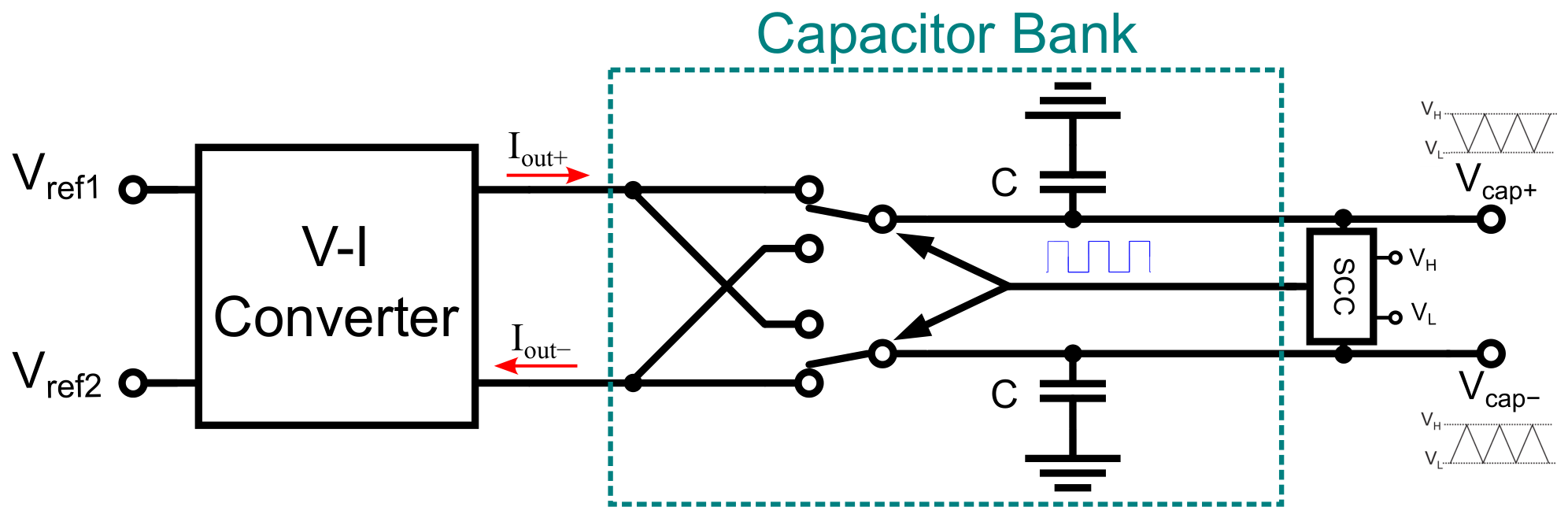
The proposed relaxation oscillator, shown in Figure 2, consists of three main subcircuits: a voltage-to-current (V-I) converter, a switchable capacitor bank, and the threshold and switching logic, referred to here as the slope control circuit (SCC). A reference input voltage is converted into an output current in order to charge/discharge the capacitors, thus producing a voltage ramp with alternating positive and negative slopes. The transition between current injection and extraction is regulated by the SCC, which monitors the voltages across the capacitors and compares them with the threshold voltages and , in order to determine when the polarity of the slope must change to form the triangular shape. The oscillator thus generates two differential signals: a triangular waveform with predefined frequency and amplitude at the capacitor terminals, and a square waveform, synchronized at the same frequency, at the output of the SCC.
Figure 2.
Block diagram of the proposed relaxation oscillator.
The oscillation frequency is determined by the following equation:
where is the transconductance value of the V-I converter, and C is the capacitance value. The oscillation frequency is thus directly proportional to the output current of the V-I converter, which sets a trade-off between power consumption and the maximum achievable frequency. Additionally, since the frequency is directly proportional to the transconductance and inversely proportional to the capacitance C, a trade-off arises between silicon area and the minimum achievable frequency. To prevent an increase in current consumption, the V-I converter was designed with a constant resistance value , and a tunable current mirror configuration to scale up or down the current delivered to the capacitors, i.e., to scale up or down the equivalent transconductance . Furthermore, a capacitor bank is used to provide coarse frequency control, thus extending the tuning range. Finally, overlapping among the three available frequency intervals is ensured by adjusting the value of . All these frequency control mechanisms will be explained next.
2.1. V-I Converter
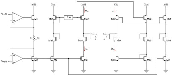
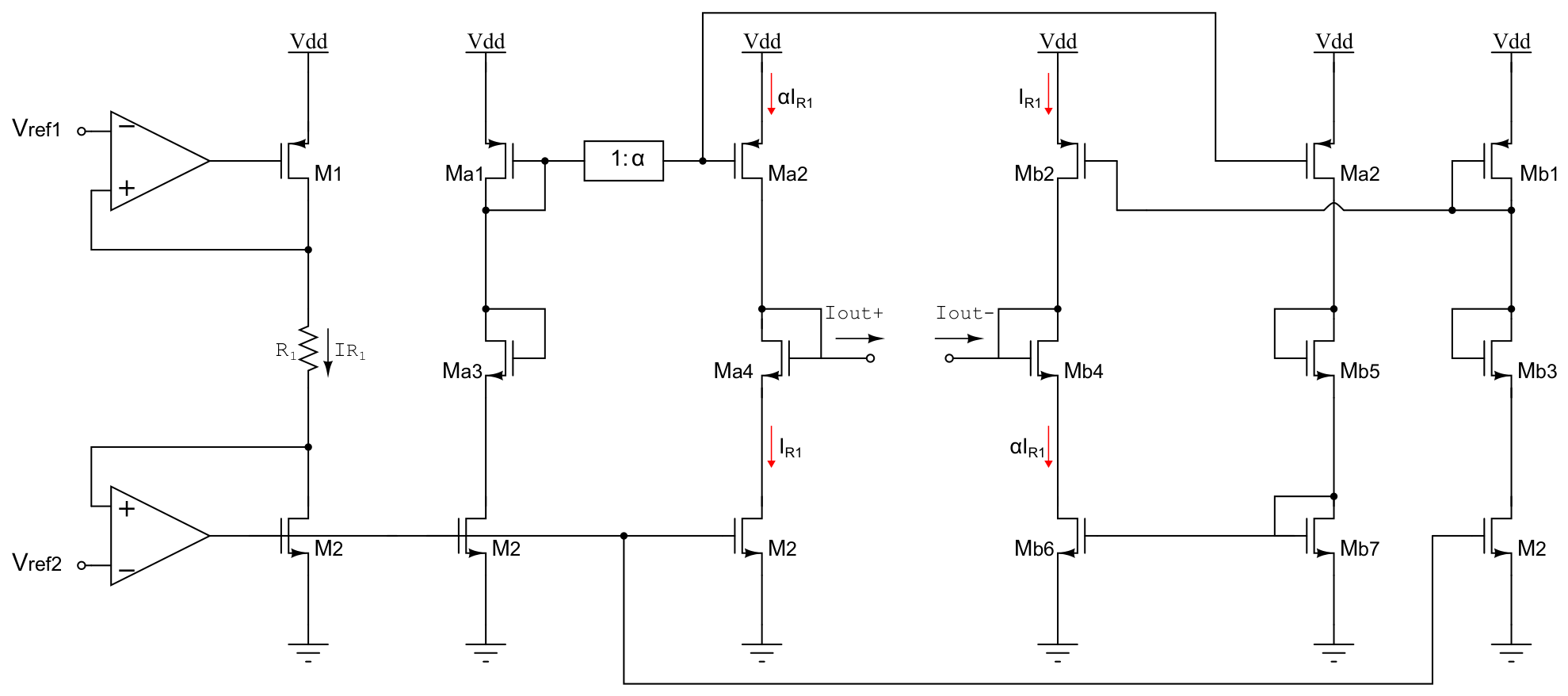
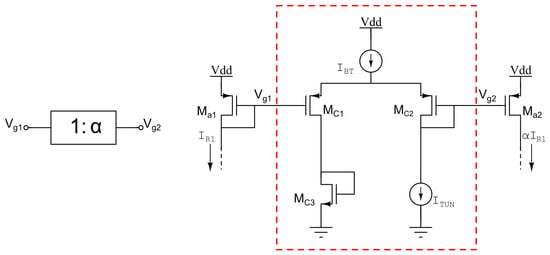
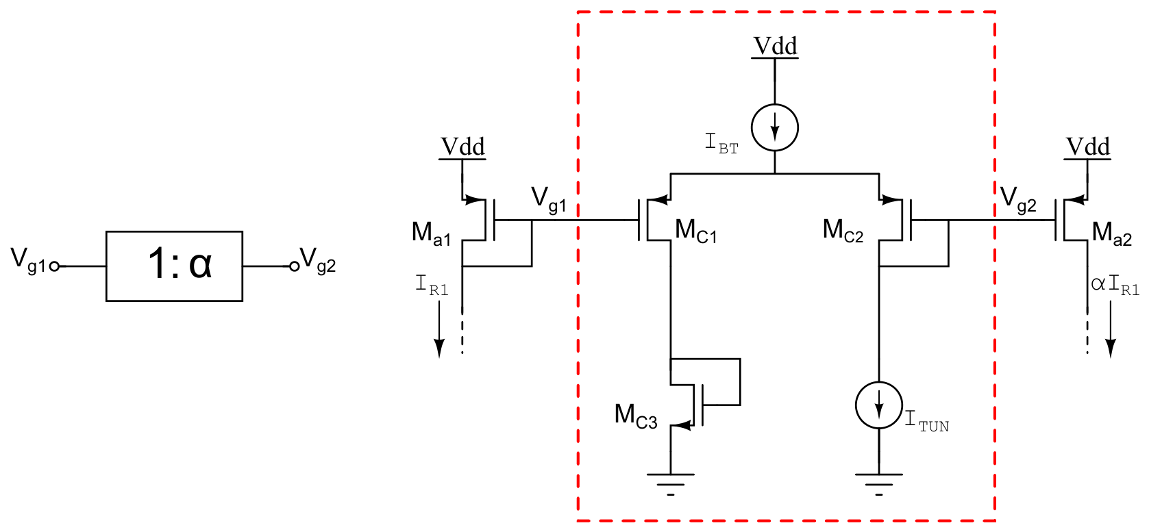
The schematic of the V-I converter is shown in Figure 3. As illustrated, it consists of two negative-feedback amplifiers that set the voltage across the terminals of resistor . If the same reference voltage is applied to both non-inverting inputs, the effective voltage drop across is minimized and the current is established in the nanoampere range. This current is subsequently replicated into additional branches via current mirrors in order to generate two output currents and , with opposite polarity and equal magnitude. The 1: block sets the copy factor of the current mirror . The value depends on the distribution of the bias current between the input transistors of a PMOS differential pair, as proposed in Ref. [19] and shown in Figure 4, where represents the tuning current. As transistors and operate in weak inversion and saturation, it can be shown that the copy factor is given by:
with . Therefore, the output currents of the V-I converter are given by:
Figure 3.
Schematic of the V-I converter.
Figure 4.
Continuously tunable current mirror.
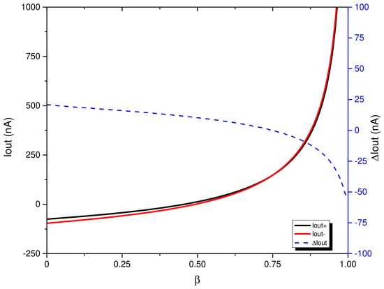
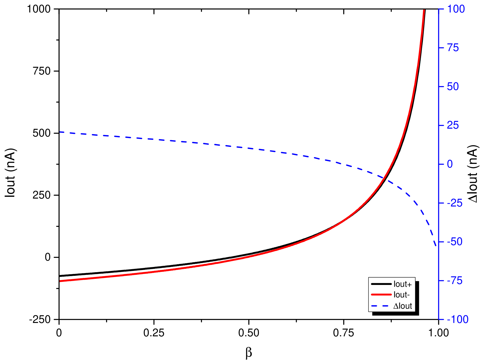
Note that always remains between 0 and 1. If = 0.5 (), ideally becomes zero because 1, causing the currents through the output branches of the V-I converter to cancel out. When (), reverses its polarity with respect to the orientation illustrated in Figure 3, and its maximum magnitude is limited by (), since the tunable current mirror attenuates the current. In contrast, when , the polarity matches that shown in Figure 3, and can become arbitrarily high as approaches unity. Figure 5 shows the output currents of the V-I converter with = 900 mV, = 100 k, = 84 nA, = 50 nA, as is swept from 0 to 1. The absolute differential error between the two output currents, which is lower than 55 nA across the entire range, is also plotted (blue dashed line). To achieve the widest frequency tuning range and avoid potential current polarity reversal caused by device mismatch, must be chosen higher than 0.5. Furthermore, should be kept below 1 to limit the maximum power consumption. For this reason, in the proposed design, the tuning parameter is restricted to the range of , which corresponds to a current sweep of 26 nA 46 nA. Finally, it is worth noting that the input voltage of the V-I converter can be increased to obtain higher values, thus resulting in higher operation frequencies. This additional degree of freedom will also be exploited in Section 2.4 by adjusting to extend the complete frequency range.
Figure 5.
Output currents of the V-I converter as a function of .
2.2. Capacitor Bank
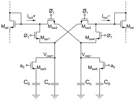
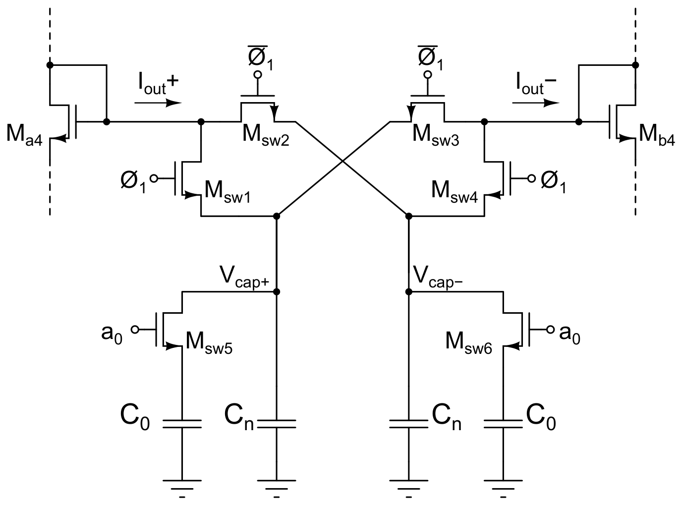
A capacitor bank was designed to achieve a wide oscillation frequency range. It consists of an array of switches and capacitors, as shown in Figure 6. Transistors – are used to reverse the slope of the triangular waveform, and are therefore controlled by the outputs of the SCC. Transistors and are controlled by a bit to establish the equivalent capacitance value, given by . When , the circuit operates with the nominal capacitance pF. Conversely, when , the capacitor pF is connected in parallel, resulting in a total capacitance of pF. This capacitance variation significantly extends the achievable frequency tuning range.
Figure 6.
Switchable capacitor bank.
2.3. Slope Control Circuit (SCC)
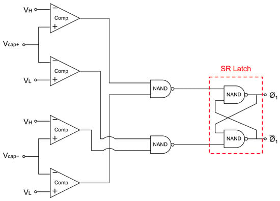
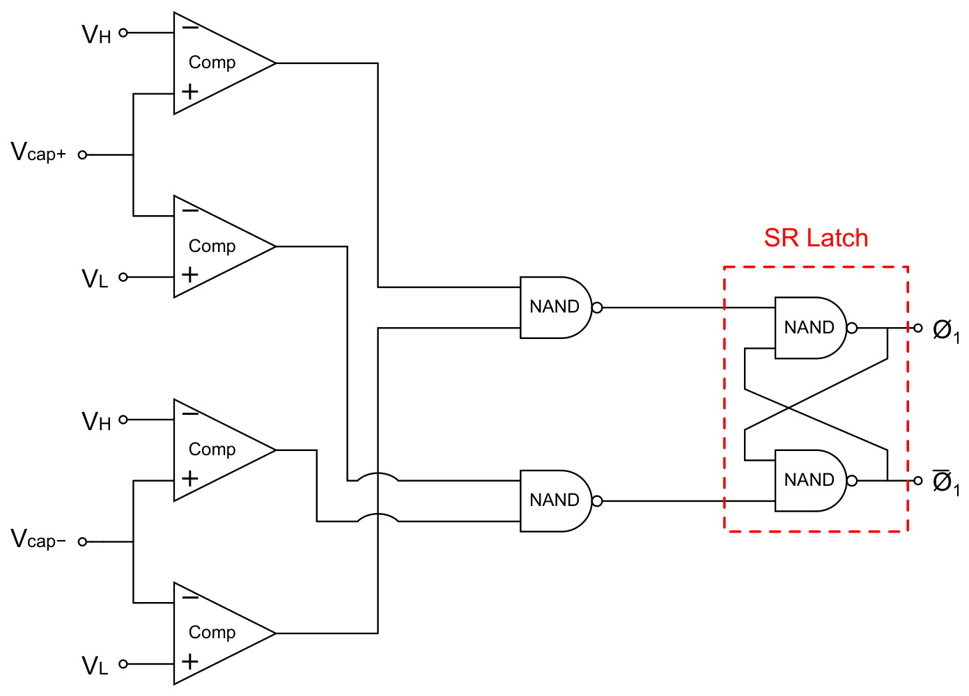
This circuit relies on four custom-designed comparators, whose inputs are connected to the capacitor terminals and , and to the threshold voltages and , as shown in Figure 7. The comparator outputs are connected to a combination of NAND gates followed by an asynchronous SR latch, whose outputs generate the control voltages required to drive the switching transistors to in Figure 6. Additionally, these outputs are differential square-wave signals synchronized in frequency with the triangular waveforms.
Figure 7.
Schematic of the slope control circuit (SCC).
2.4. Relaxation Oscillator Simulation Results
The proposed relaxation oscillator was implemented in a 0.18 m CMOS process with a 1.8 V supply voltage. Considering all the incorporated frequency control mechanisms, the oscillation frequency is given by:
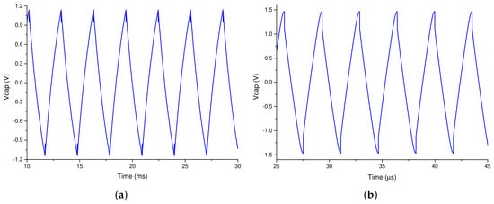
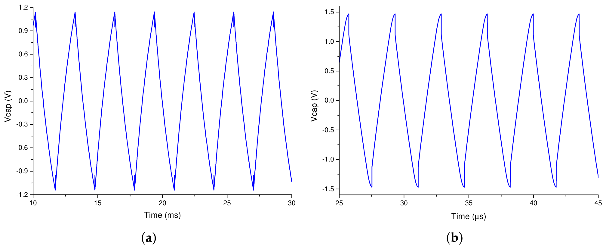
Continuous fine frequency tuning is achieved through the current ratio , with = 50 nA, whereas coarse tuning is performed via the digital bit . Although the adjustment of the differential voltage could also function as an additional fine-tuning mechanism, in this specific design, was restricted to two discrete voltage levels to extend frequency operation up to 300 kHz. The key component values and design parameters are summarized in Table 1, and Table 2 shows the different frequency range configurations. To verify the circuit operation, post-layout simulations were performed. The oscillator occupies an area of 0.19 and consumes 10.7 W in the worst case, i.e., at maximum frequency. Figure 8 shows the steady-state differential output waveforms under two extreme conditions: for a tuning current 26 nA ( = 0.52), with 900 mV and = 1, which results in the minimum frequency f = 300 Hz; and for a tuning current 46 nA ( = 0.92), with = 850 mV and , which results in the maximum frequency of f = 300 kHz. The average peak-to-peak output voltage is 1.02 V. Table 3 summarizes the main characteristics of the relaxation oscillator.
Table 1.
Component values and design parameters.
Table 2.
Frequency tuning range configurations.
Figure 8.
Triangular wave generated at (a) 300 Hz and (b) 300 kHz.
Table 3.
Characteristics of the relaxation oscillator.
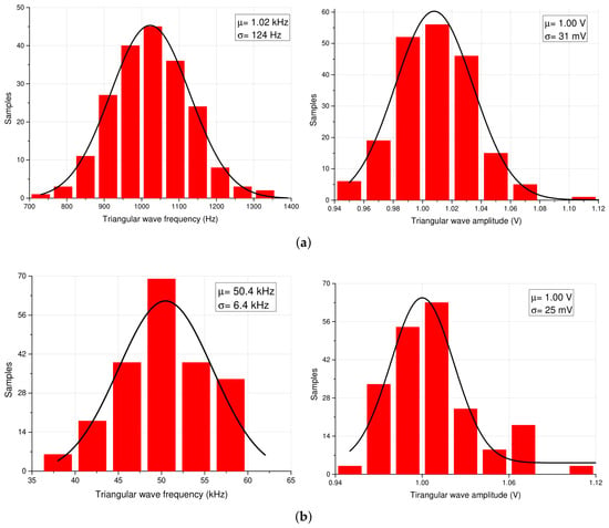
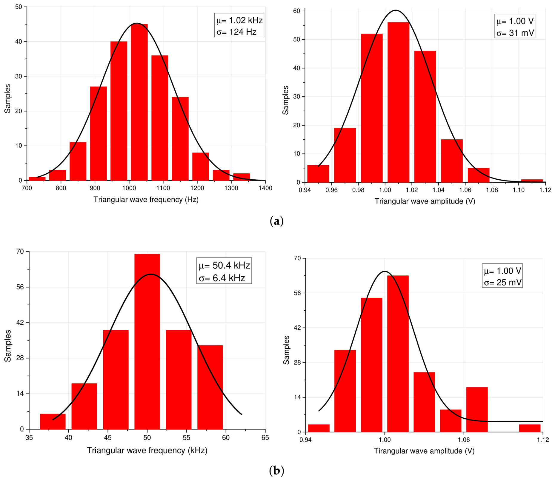
To validate robustness, a 200-run Monte Carlo simulation was performed at 1 and 50 kHz, and the results are shown in Figure 9. As observed, the amplitude of the differential triangular waveform remains almost constant at both operating frequencies. At 1 kHz, the mean amplitude is 1 V with a standard deviation of 31 mV, while at 50 kHz, the same mean value of 1 V is maintained with a slightly lower standard deviation of 25 mV. Regarding frequency, the mean values are 1.02 kHz and 50.4 kHz, with standard deviations of 124 Hz and 6.4 kHz, respectively. In both cases, the mean frequency remains close to the intended operating value, although the circuit exhibits frequency dispersion due to process and mismatch variations. However, this frequency deviation can be readjusted after fabrication via the tuning current .
Figure 9.
Monte Carlo simulations for frequency and amplitude of the triangular wave at (a) 1 kHz and (b) 50 kHz.
3. Tunable Sixth-Order Gm-C BPF
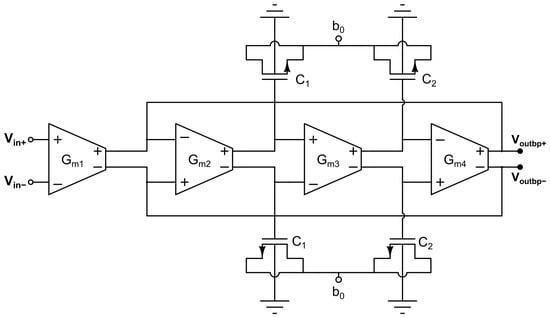
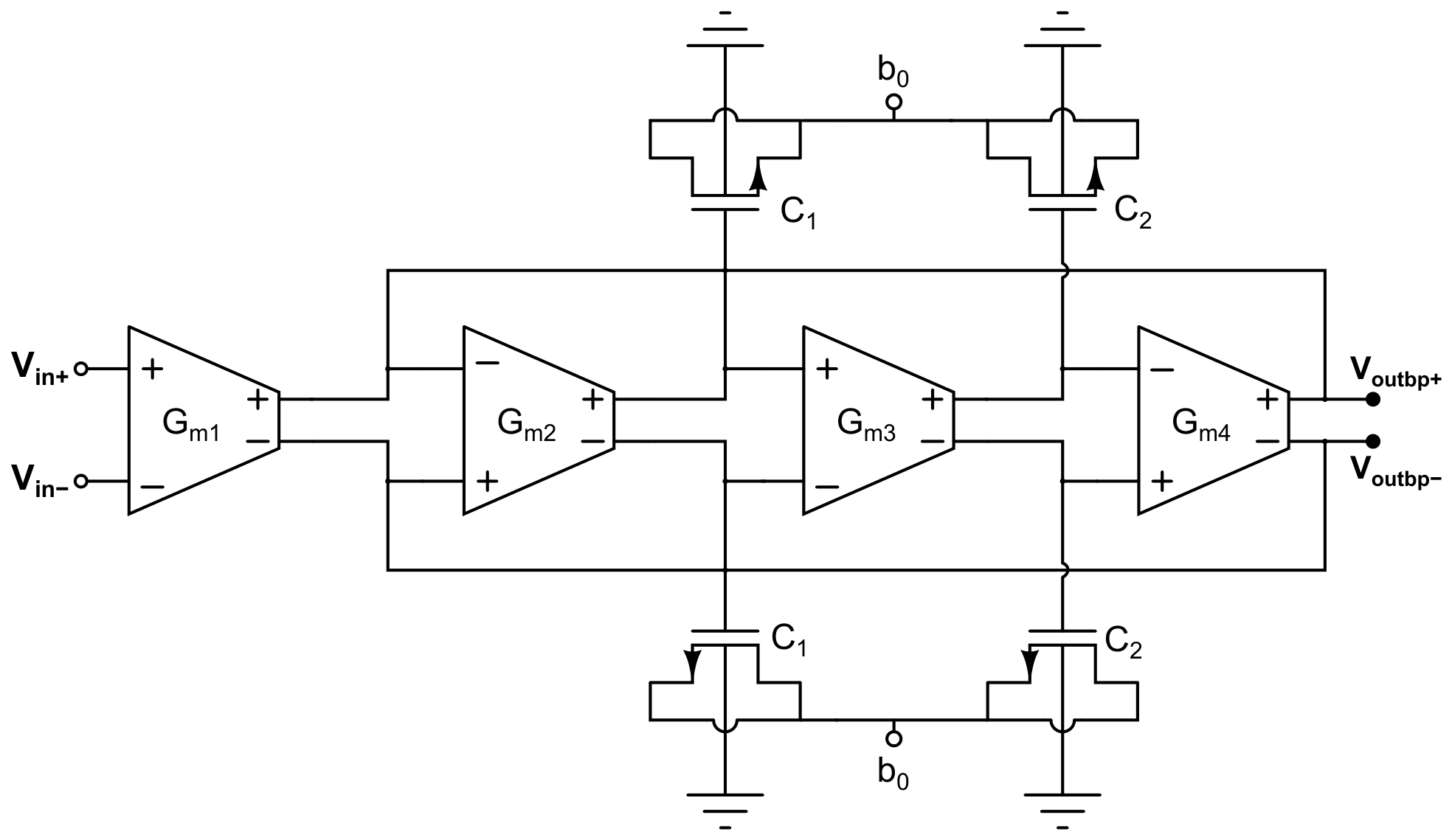
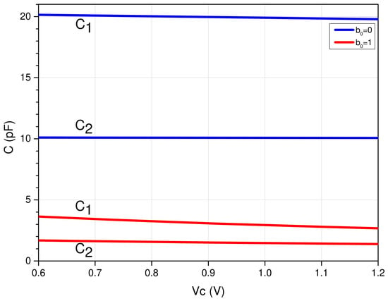
The linearization stage of the proposed sine waveform generator is a sixth-order bandpass filter based on the fully differential Tow–Thomas biquad shown in Figure 10. Each biquadratic section consists of four fully differential low-Gm OTAs and a programmable NMOS capacitor bank that selects the operation frequency range through a control bit . For , pF and pF, providing a center-frequency tuning range from 10 to 50 kHz. When , the capacitances are increased to pF and pF, allowing the center frequency to be tuned from 1 to 10 kHz. Figure 11 shows the capacitance–voltage characteristics of and for both states of the digital control bit . The dimensions of these NMOS capacitors are = 50 m/49 m and = 24.8 m/49 m.
Figure 10.
Fully differential Tow–Thomas Gm-C biquad.
Figure 11.
Capacitance–voltage characteristics of and .
The transfer function of the biquad is given by:
The gain is determined by the ratio , while the quality factor Q and the center frequency are given by:
Synchronous tuning is used across all three biquads to achieve a steep roll-off characteristic, which is essential for effectively suppressing the undesired frequency components generated by the relaxation oscillator. Furthermore, all transconductance values are set to the same Gm value, so the filter gain is unity, and Q and are given by:
In this design, frequency tuning relies solely on the OTA transconductance. By choosing , the quality factor was set to Q = . The relatively low Q value makes the system tolerant to small frequency alignment errors between the signal frequency f and the center frequency . For instance, from the transfer function of the sixth-order filter, it can be shown that a ±5% misalignment results in a gain drop of less than 0.3 dB, i.e., in an amplitude attenuation of about 3%. Meanwhile, the sixth-order roll-off of the cascaded biquadratic stages ensures, as already mentioned, the filtering of high-order harmonics. Note that triangular waveforms contain exclusively odd harmonics, so the closest non-desired frequency component of the input signal is at , which will be suppressed by the BPF stopband, as shown in the next Section.
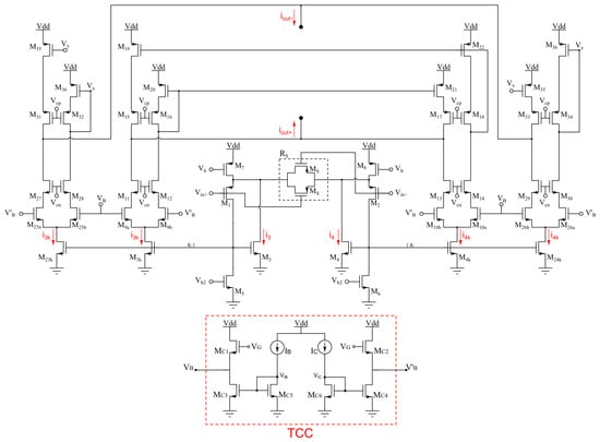
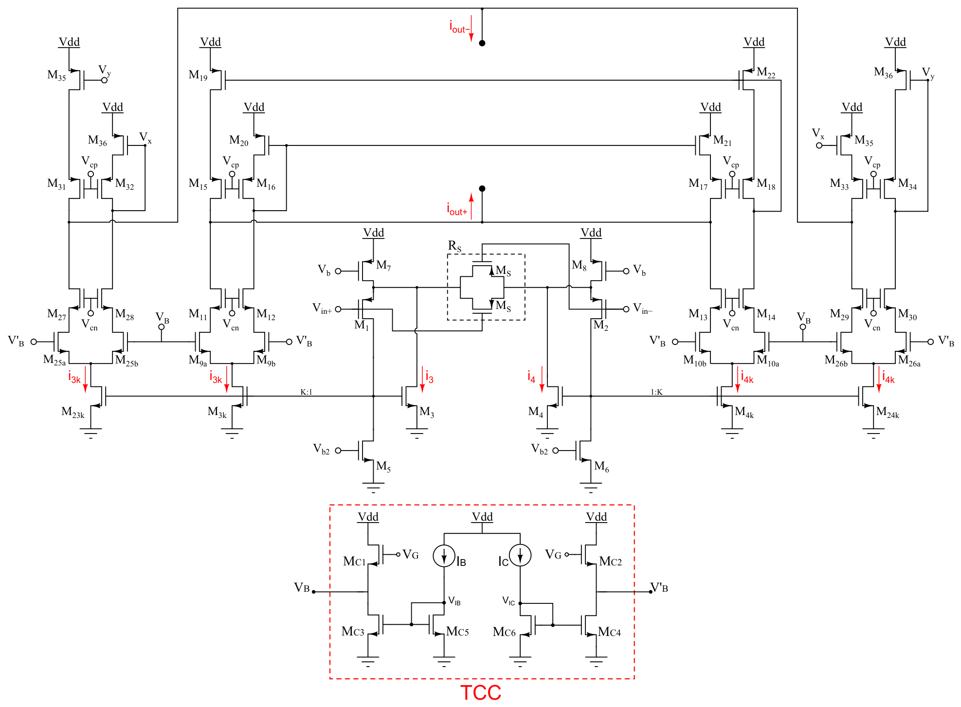
The low-Gm OTA is a fully differential version of the architecture proposed in Ref. [20], as shown in Figure 12. It employs current cancelation by splitting the differential output current of a transconductor into four paths and subtracting the resulting currents at the outputs. This technique results in transconductance values ranging from a few units to several hundreds of nS. A transconductance control circuit (TCC) generates the bias voltages and through the ratio m between a control current and a bias current . The equivalent transconductance of the OTA is given by:
where is the differential input voltage, K is the gain of the current mirrors , is the equivalent resistance of the degeneration transistors , and is the current ratio.
Figure 12.
Fully differential low-Gm tansconductor.
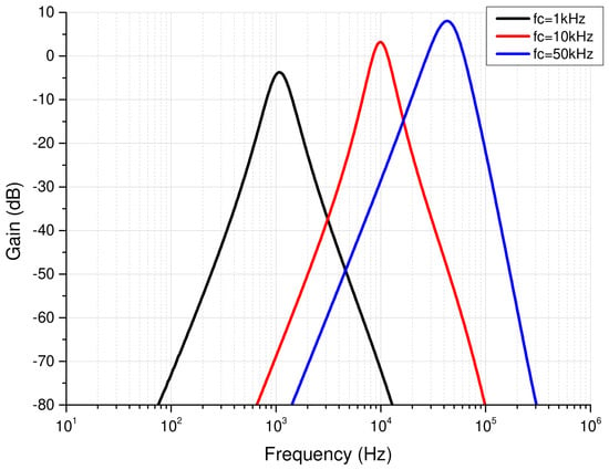
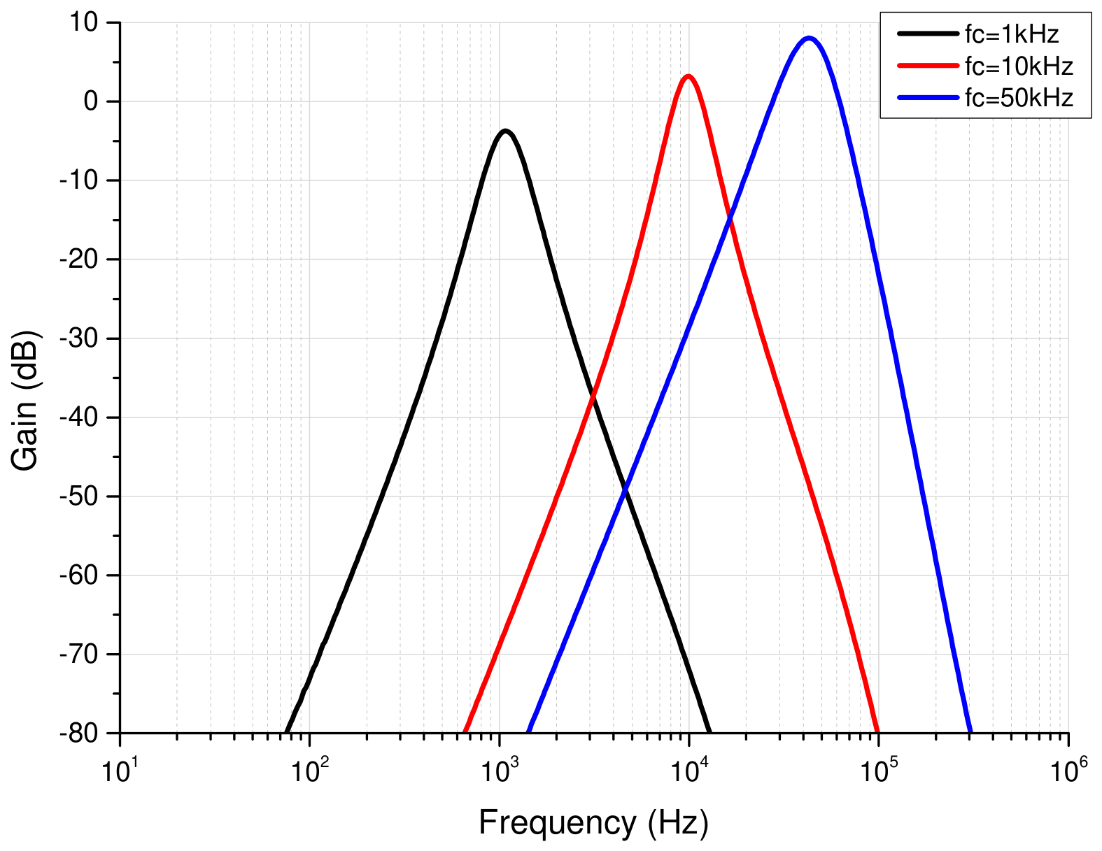
was set to 25 nA and varies from 28 nA to 2 A (), so the transconductance of each OTA in the BPF is tuned from 23 to 775 nS. In this way, the center frequency of the filter can be tuned from 1 to 50 kHz. Figure 13 shows the frequency response of the filter at 1, 10, and 50 kHz. The frequency range configurations are shown in Table 4, while Table 5 summarizes the main BPF characteristics. The power consumption remains under 16 W across the entire frequency tuning range. Note that the use of low-Gm OTAs to accommodate the low-frequency requirements of the system without demanding large on-chip capacitors also limits the maximum achievable center frequency.
Figure 13.
Frequency response of the BPF.
Table 4.
Frequency tuning range configurations of the BPF.
Table 5.
Characteristics of the BPF.
4. Proposed CMOS Sine Waveform Generator
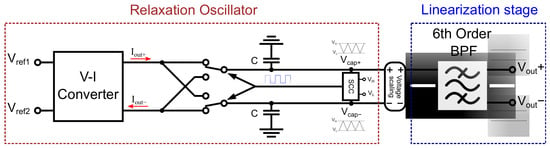
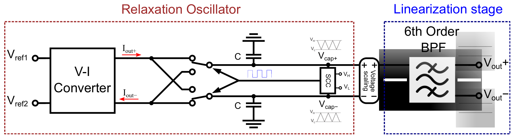
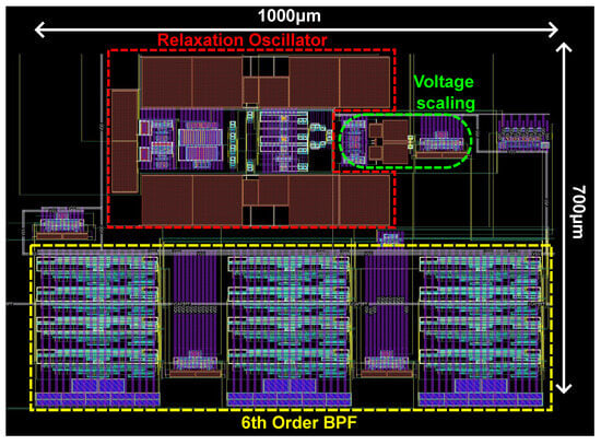
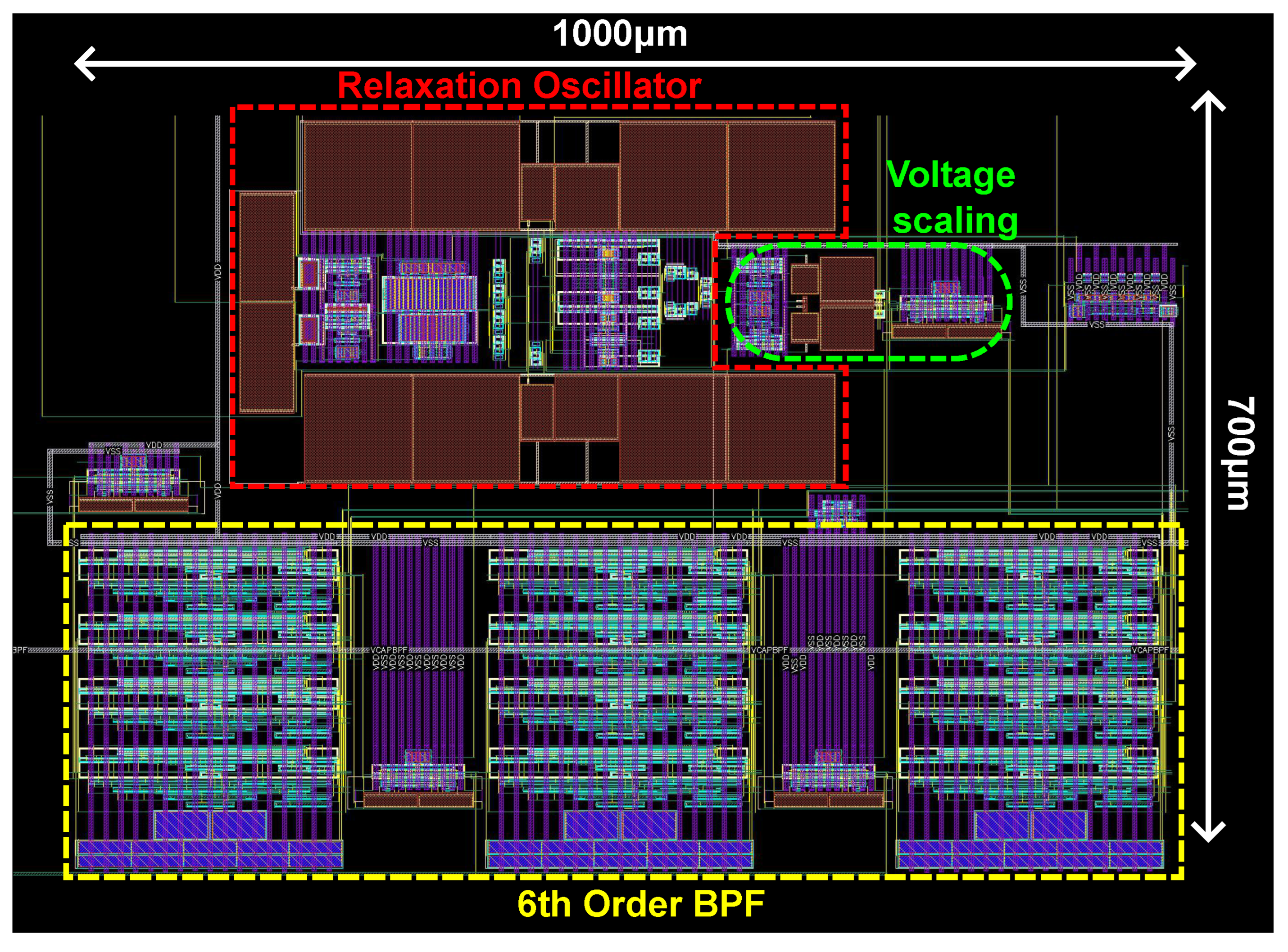
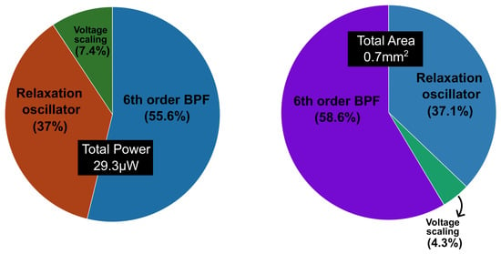
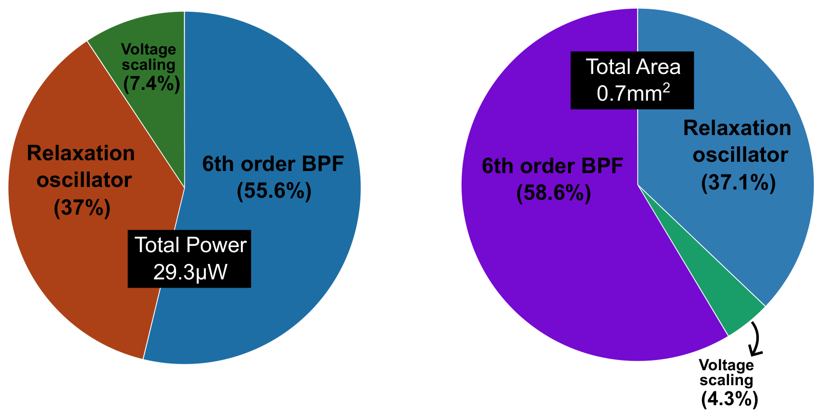
The CMOS sine waveform generator was implemented by cascading the relaxation oscillator and the sixth-order Gm-C bandpass filter, which serves as the linearization stage. As shown in Figure 14, a voltage scaling stage, which consists of a capacitive attenuator and a low-power buffer, was placed at the output of the oscillator, thus avoiding saturation of the BPF and non-linear effects, which would otherwise compromise the linearization process. The complete circuit layout, designed in 0.18 m CMOS technology, is shown in Figure 15. It occupies a total area of 0.7 and consumes 29.3 W from a 1.8 V supply voltage. The power and area breakdown are shown in Figure 16. The relaxation oscillator only demands a 37% share for both metrics while providing a triangular output with a wide three-decade frequency tuning range. The power and area consumption are dominated by the sixth-order BPF, due to the circuit complexity of high-order active filters. As already mentioned, the maximum center frequency is limited by the low-power, low-Gm OTAs used for low-frequency operation. In this prototype, no tuning mechanism was integrated to adjust the passive components in the relaxation oscillator, specifically , which is a high-resistivity polysilicon resistor. While process variations in these components shift the available tuning range of the triangular wave after fabrication, they do not restrict the tuning range of the whole sine waveform generator. To carry out post-layout simulations, the frequency sub-range was first set by the control bits (): (1, 0) from 1 to 10 kHz, and (0, 1) from 10 to 50 kHz. Next, the target output frequency was set by sweeping the tuning current of the relaxation oscillator. Once the target frequency was established, the BPF center frequency was aligned by adjusting its bias current until reaching a maximum output amplitude voltage. Table 6 shows the frequency range configurations of the sine waveform generator. The reference voltage was kept constant at 900 mV. In order to show how the calibration process can be automated in future implementations, a digitally controlled tuning scheme is conceptually proposed in Appendix A.
Figure 14.
Sine waveform generator block diagram.
Figure 15.
Layout of the proposed sine waveform generator.
Figure 16.
Power and area breakdown of the proposed sine waveform generator.
Table 6.
Frequency tuning range configurations of the sine waveform generator.
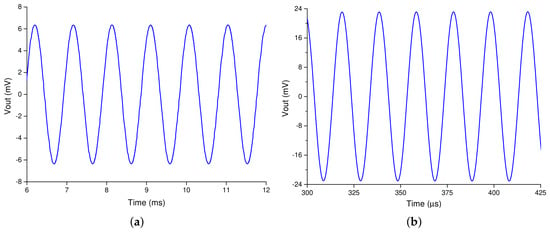
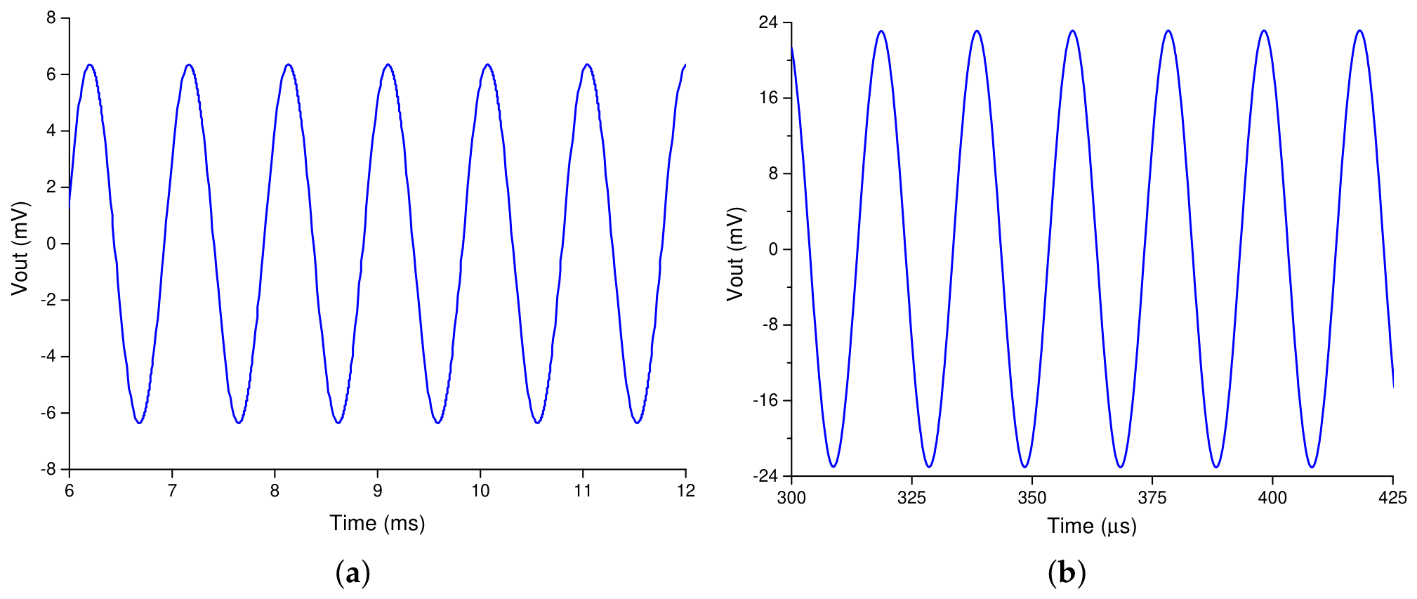
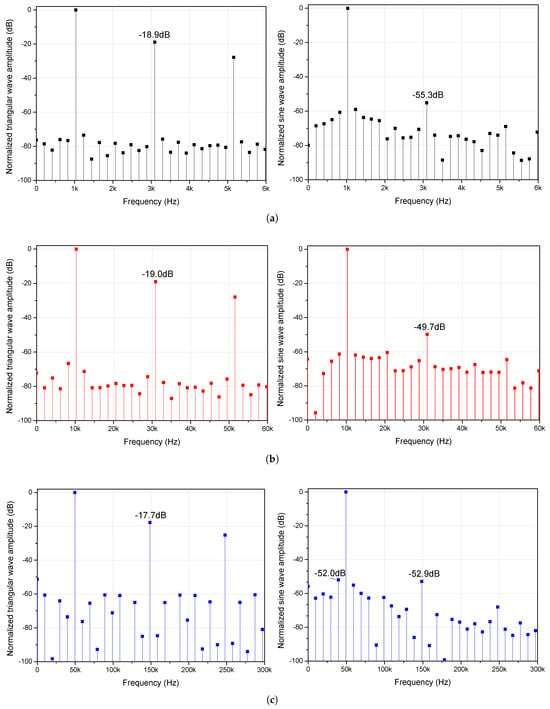
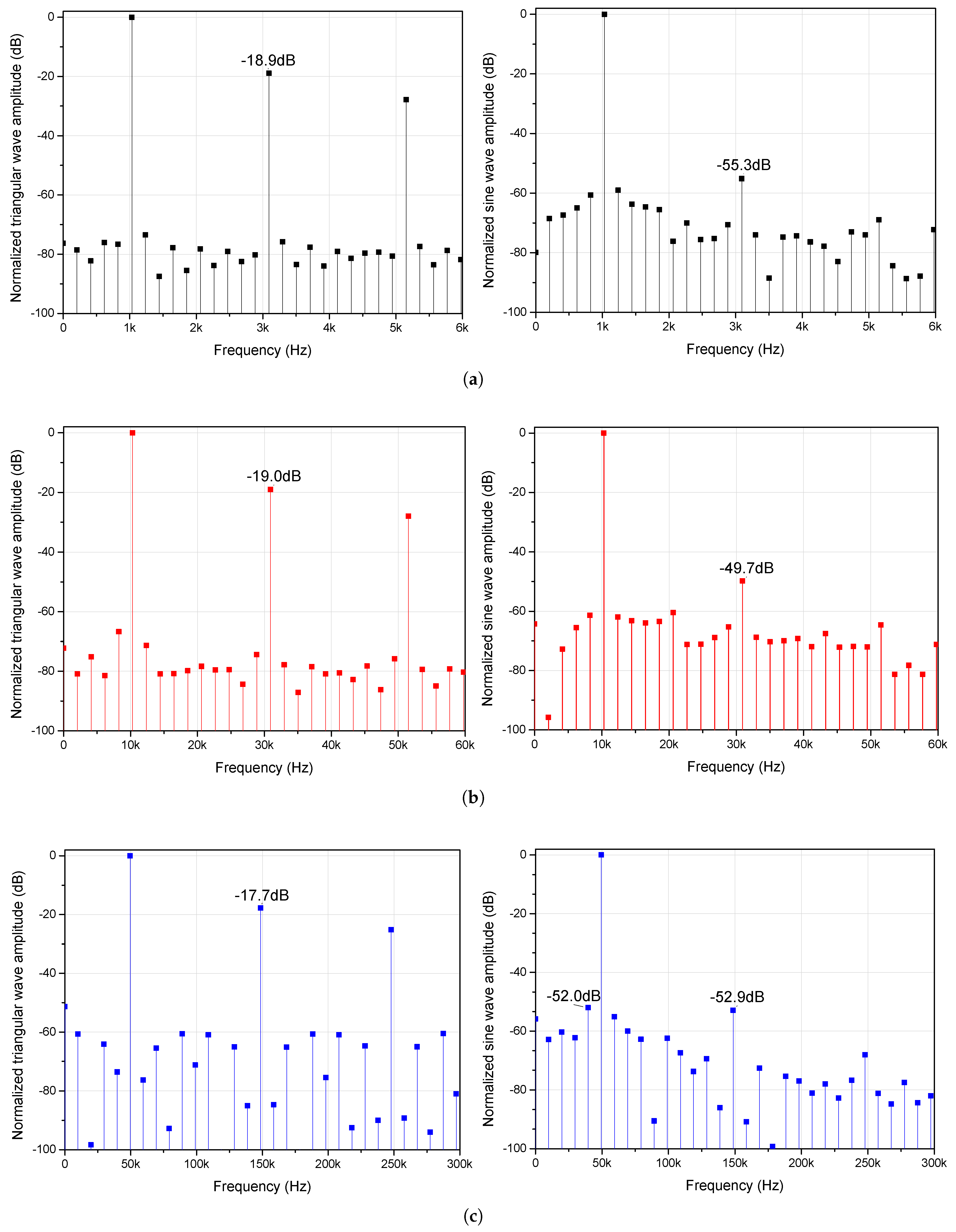
Figure 17 shows the steady-state differential output signal of the generator at 1 and 50 kHz, confirming the correct sine waveform generation. In order to demonstrate the linearity improvement achieved by the BPF, Figure 18 compares the frequency spectra of the triangular and sinusoidal signals at several frequency settings. As shown, the third harmonic is reduced by more than 30 dB by the linearization stage. Note that, due to the fully differential architecture, even harmonics are virtually eliminated. The worst-case THD is −48.8 dB at 10 kHz with 32 , whereas the lowest THD of −55 dB is achieved at 1 kHz with 12 output voltage. Alternative filter design techniques can be explored in the future to extend the operation frequency of the sine waveform generator without compromising the silicon area or power efficiency. In such a scenario, in the relaxation oscillator should be replaced by a digitally programmable resistor bank to compensate for process variations across the extended frequency range.
Figure 17.
Time response of the sine waveform generator at (a) 1 kHz and (b) 50 kHz.
Figure 18.
Frequency spectrum of the triangular wave and the output sine wave at (a) 1 kHz, (b) 10 kHz and (c) 50 kHz.
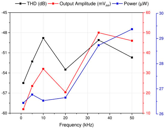
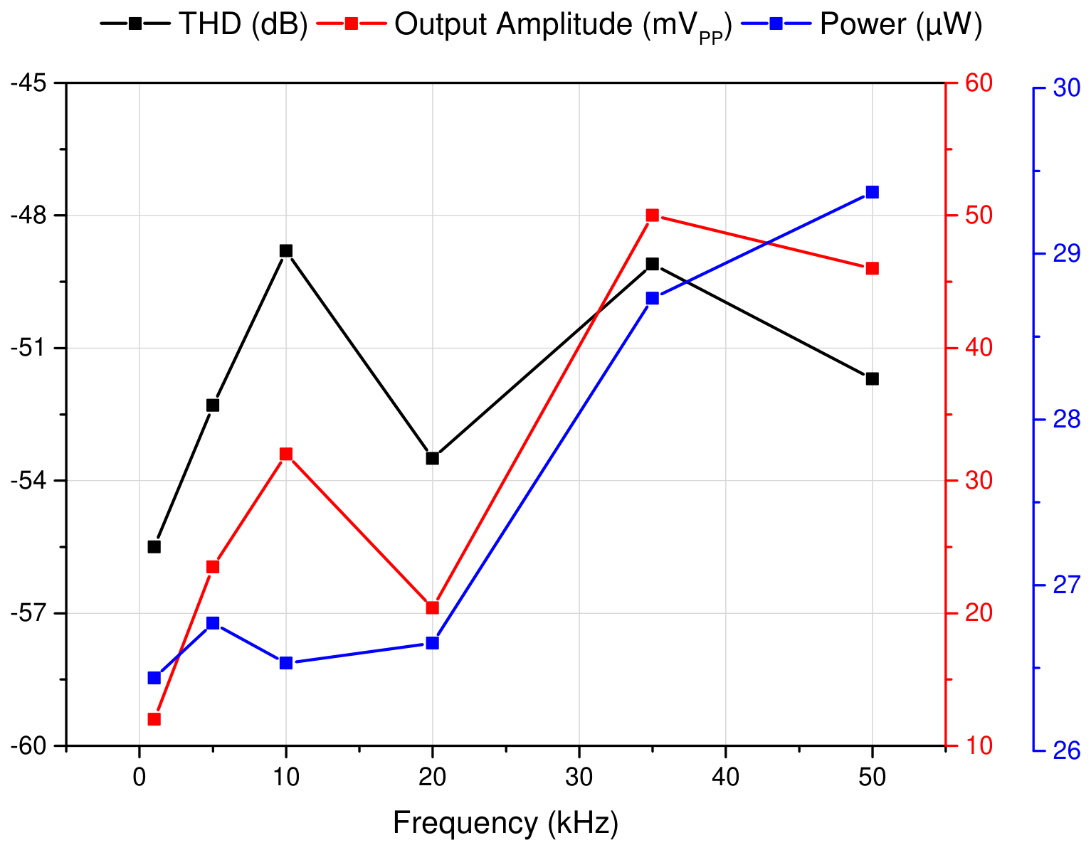
The output amplitude, THD, and power consumption of the sine waveform generator as a function of the operating frequency are shown in Figure 19. The output amplitude ranges from 12 to 50 , with a THD lower than −48 dB throughout the whole frequency range. Although power consumption slightly increases with frequency, it remains below 29.3 W in all cases.
Figure 19.
THD, output amplitude and power consumption vs. frequency.
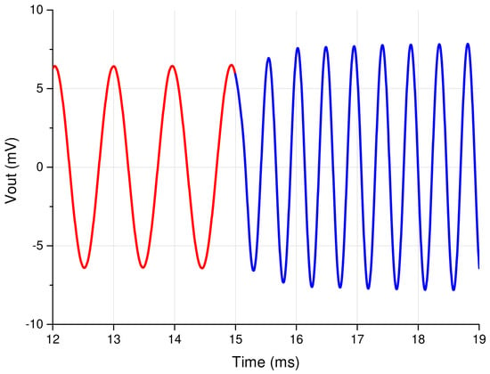
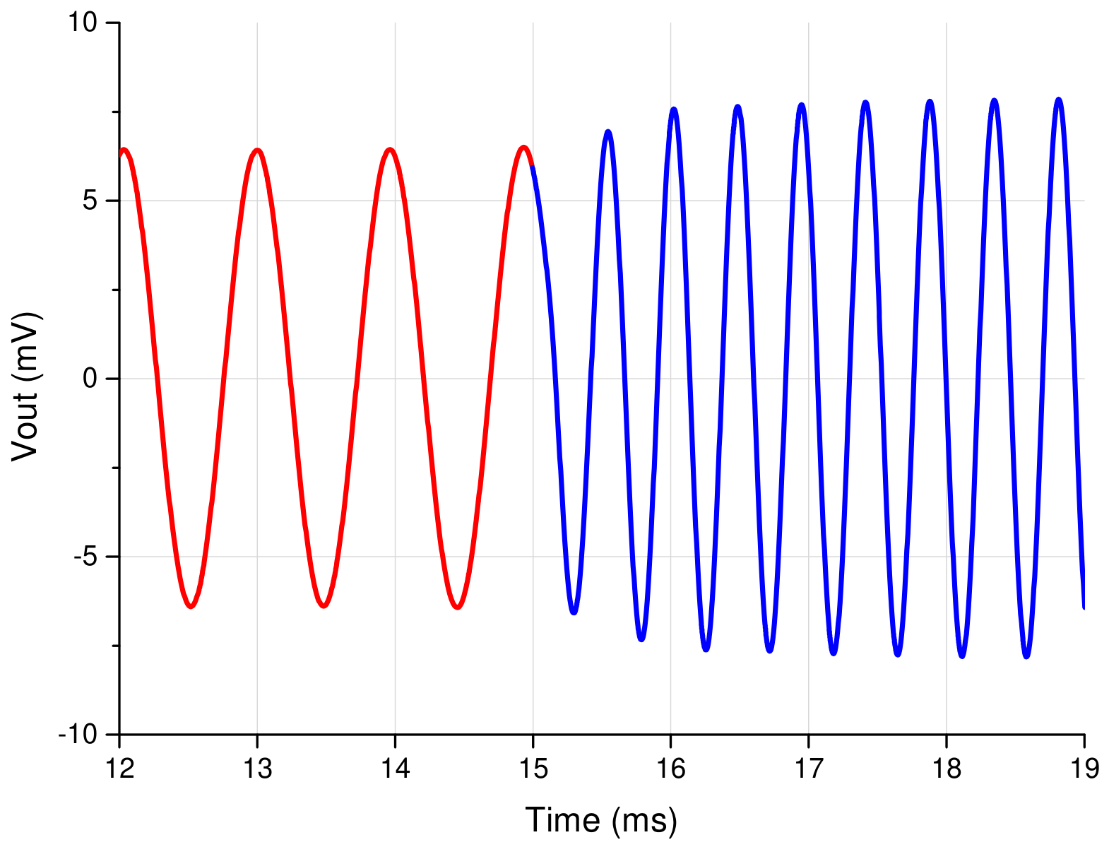
To evaluate the dynamic response between adjacent frequency steps during spectroscopy, Figure 20 illustrates the settling behavior for a 1 to 2 kHz step. This transition represents the most critical scenario in terms of absolute settling time, as lower-frequency signals inherently require longer time intervals to complete the necessary cycles for amplitude stabilization. After the change in the control signals, the differential sinusoidal output achieves steady-state operation within approximately 1.6 ms, which corresponds to about three signal cycles, enabling step-by-step impedance spectroscopy with minimal delay between measurement points.
Figure 20.
Dynamic settling response for a frequency step from 1 to 2 kHz.
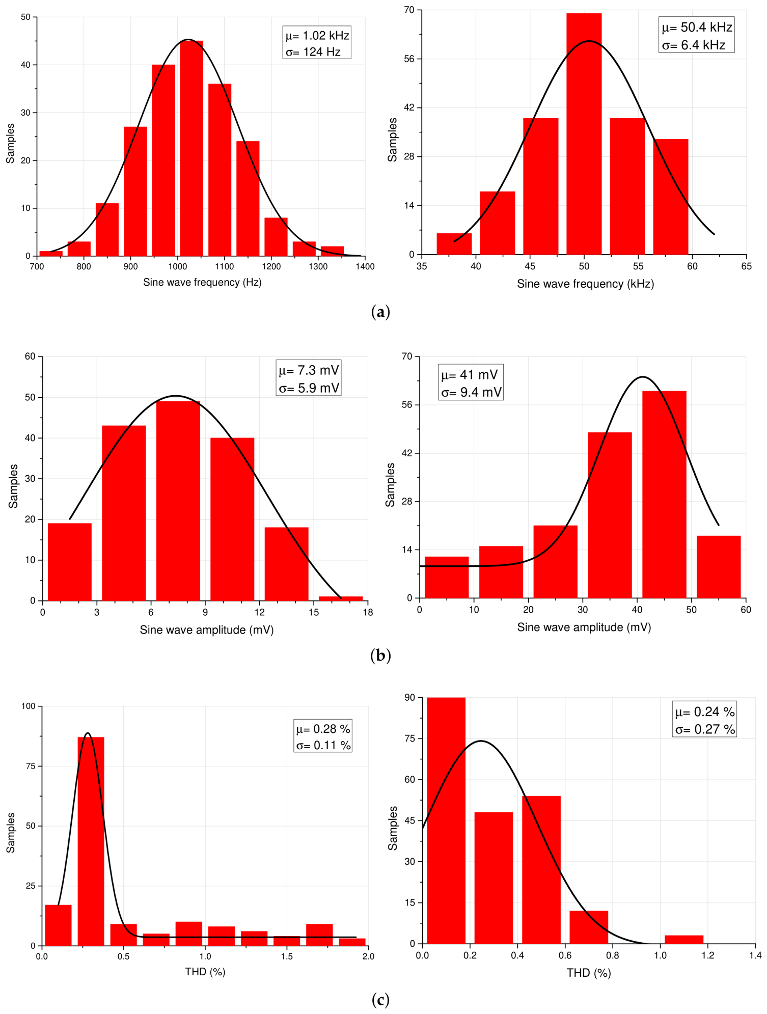
In order to validate the robustness of the sine waveform generator, a 200-run Monte Carlo simulation was performed at 1 and 50 kHz. The results are shown in Figure 21. At 1 kHz, the sinusoidal amplitude has a mean value of 7.3 mV with a standard deviation of 5.9 mV, whereas at 50 kHz the mean value increases to 41 mV with a standard deviation of 9.4 mV. While this amplitude variation could be corrected after fabrication by adjusting the ratio of the BPF, such calibration is not incorporated in the current design and should be addressed in future implementations. The mean THD remains below 0.3%, decreasing from 0.28% at 1 kHz to 0.24% at 50 kHz, with a standard deviation of 0.11% and 0.27%, respectively. Finally, the frequency distribution of the sine waveform generator is determined by the frequency distribution of the relaxation oscillator, so the mean and standard deviation values are the same as those obtained for the triangular waveform in Section 2: a mean value of 1.02 kHz with 124 Hz standard deviation at 1kHz, and a mean value of 50.4 kHz with 6.4 kHz standard deviation at 50 kHz. The frequency tuning mechanism provided by the tuning current of the relaxation oscillator enables precise post-fabrication adjustment to compensate for this dispersion.
Figure 21.
Monte Carlo simulations for the sine wave at 1 kHz and 50 kHz of (a) frequency, (b) amplitude and (c) THD.
Regarding PVT, the proposed low-power sine waveform generator is designed for energy-constrained applications and is intended to operate from a regulated supply voltage to mitigate the impact of supply fluctuations. As for global process and temperature variations, evaluating the generator under fixed open-loop control parameters does not reflect actual operation, since the induced frequency drift is dynamically compensated once integrated into a closed-loop system. The block-level architecture of the master–slave automatic tuning scheme proposed in Appendix A illustrates how this dynamic compensation can be integrated in the final application. However, as this tuning loop is a high-level conceptual proposal, full PVT validation of the closed-loop system is beyond the scope of the present post-layout simulation study. A comparison between the proposed design and recent state-of-the-art sine waveform generators is summarized in Table 7. For Refs. [17,21], which also integrate an output current driver, the silicon area and power consumption of the signal generator were estimated separately to enable a fair comparison. The analog solutions presented in Refs. [17,22] provide a wider frequency tuning range than the proposed generator, at the cost of higher power consumption. In particular, the design in Ref. [17] exhibits higher distortion and consumes approximately 5.5 times more power, while the implementation in Ref. [22] achieves low distortion at a significantly higher output amplitude but consumes several orders of magnitude more power. Furthermore, the design in Ref. [22], which also relies on a relaxation oscillator, requires a massive external capacitor to reach low frequencies, which heavily penalizes the system’s portability. Digital approaches, such as the DDS in Ref. [23] or the Delta-Sigma Modulated Look-Up Table (-LUT) architectures in Refs. [21,24], generally exhibit lower distortion figures. The generator in Ref. [21] offers a linearity comparable to our proposal, but features a narrower frequency tuning range (1:5 vs. 1:50). Although the linearity in Ref. [24] stands out, and its power consumption is also slightly lower, its operation is limited to a single 20 kHz frequency. Finally, the design in Ref. [23] provides a wider frequency tuning range and superior linearity at a high output amplitude, but at the cost of a power consumption increase of more than one order of magnitude with respect to this work. In summary, the proposed sine waveform generator shows a good trade-off between frequency programmability, linearity, and power consumption, and is therefore highly suitable for energy-constrained portable medical applications within the kilohertz range.
Table 7.
Performance comparison of sine waveform generators.
5. Conclusions
In this paper, a fully integrated CMOS sine waveform generator based on a relaxation oscillator and a sixth-order Gm-C band-pass filter was presented. The proposed circuit was designed in a 0.18 m CMOS process and operates from a 1.8 V supply voltage. Post-layout simulation results show that the relaxation oscillator generates a differential triangular waveform with a wide frequency tuning range from 300 Hz to 300 kHz, achieved through the combined adjustment of a control current, a reference voltage, and a switchable capacitor bank. The sixth-order Gm-C bandpass filter converts the triangular waveform into a sinusoidal signal with a frequency tuning range from 1 to 50 kHz and a THD lower than 0.36%. Although the maximum center frequency of the BPF is constrained by the low-Gm OTAs designed for low-frequency operation, the use of large on-chip capacitors is avoided, and power consumption is kept to a minimum. The complete sine waveform generator consumes less than 30 W power, making it suitable for portable BioZ spectroscopy applications within the kilohertz range, such as impedance pneumography-based respiratory monitoring, tissue composition characterization, or cellular health assessment.
Author Contributions
Conceptualization, E.I.B.d.l.C. and M.T.S.-P.; methodology, E.I.B.d.l.C. and B.C.; software, E.I.B.d.l.C. and J.D.S.C.; validation, E.I.B.d.l.C., J.D.S.C. and M.T.S.-P.; formal analysis, M.T.S.-P.; investigation, E.I.B.d.l.C. and N.M.; resources, M.T.S.-P. and N.M.; data curation, E.I.B.d.l.C. and J.D.S.C.; writing—original draft preparation, E.I.B.d.l.C.; writing—review and editing, M.T.S.-P., B.C. and N.M.; visualization, E.I.B.d.l.C.; supervision, M.T.S.-P. and B.C.; project administration, M.T.S.-P. and N.M.; funding acquisition, M.T.S.-P. and N.M. All authors have read and agreed to the published version of the manuscript.
Funding
This work was supported by SECIHTI through the Doctoral Grants 24670 and 1155828, and the Research Project CBF-2025-I-3792, and by the State Research Agency of the Ministry of Science and Innovation through the Project PID2022-138785OB-I00/AEI/10.13039/501100011033/FEDER, UE.
Data Availability Statement
The original contributions presented in this study are included in the article. Further inquiries can be directed to the corresponding authors.
Conflicts of Interest
The authors declare no conflicts of interest.
Appendix A. Automatic Tuning Scheme
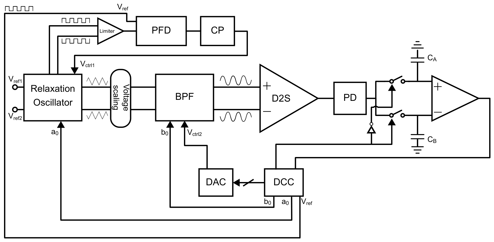
To enable continuous frequency sweeping for spectroscopy applications, a high-level master–slave automatic tuning architecture with a digital control circuit (DCC) is conceptually proposed, as shown in Figure A1. The DCC provides the reference clock signal that sets the frequency of the whole circuit. Internally, the DCC features a digital step-counter to sweep the frequency of the clock reference, and a magnitude comparator continuously evaluates this counter to automatically set the sub-band selection bits () according to the corresponding frequency range: (1, 0) from 1 to 10 kHz, and (0, 1) from 10 to 50 kHz. Consequently, the DCC manages both the fine-tuning steps and the coarse sub-band selection. The relaxation oscillator acts as the master block, while the BPF functions as the slave, dynamically tracking the master’s frequency.
The master loop is based on an analog phase-locked loop (PLL) to establish the oscillation frequency of the triangular signal. The differential square-wave output provided by the relaxation oscillator ( and in Figure 7), which is synchronized with the triangular signal, is converted via a limiter into a single-ended digital clock with clean, rail-to-rail transitions, and is then fed into the PFD and compared with . A charge pump (CP) at the output of the PFD provides the analog control voltage required to adjust , forcing the triangular wave to precisely lock onto .
As for the slave loop, the fully differential output of the BPF is first processed by a differential-to-single-ended (D2S) converter followed by a peak detector (PD) to extract its amplitude envelope (). A dual sample-and-hold network operates in an alternating configuration: one capacitor tracks and stores the current peak voltage, while the second capacitor holds the voltage from the previous state. An analog comparator evaluates both nodes and delivers a binary decision to the digital control logic. Following a successive-approximation register (SAR) algorithm, the digital logic adjusts a digital-to-analog converter (DAC) to tune the BPF. By locking the DAC code at the point of maximum output amplitude, the system guarantees synchronization between the triangular signal and the BPF across the entire frequency sweep.
Figure A1.
Master–slave automatic tuning architecture.
References
- York, S.L.; Ward, L.C.; Czerniec, S.; Lee, M.J.; Refshauge, K.M.; Kilbreath, S.L. Single frequency versus bioimpedance spectroscopy for the assessment of lymphedema. Breast Cancer Res. Treat. 2009, 117, 177–182. [Google Scholar] [PubMed]
- Khalil, S.F.; Mohktar, M.S.; Ibrahim, F. The Theory and Fundamentals of Bioimpedance Analysis in Clinical Status Monitoring and Diagnosis of Diseases. Sensors 2014, 14, 10895–10928. [Google Scholar] [CrossRef] [Scilit] [PubMed]
- Rincon, K.; Shah, P.; Ramella-Roman, J.; Bhansali, S. A Review of Engineering Approaches for Lymphedema Detection. IEEE Rev. Biomed. Eng. 2016, 9, 79–90. [Google Scholar] [CrossRef] [Scilit] [PubMed]
- Mayne, K.J.; Shemilt, R.; Keane, D.F.; Lees, J.S.; Mark, P.B.; Herrington, W.G. Bioimpedance indices of fluid overload and cardiorenal outcomes in heart failure and chronic kidney disease: A systematic review. J. Card. Fail. 2022, 28, 1628–1641. [Google Scholar] [CrossRef] [Scilit] [PubMed]
- Bailleul, A.; De Gannes, F.P.; Pirog, A.; N’kaoua, G.; D’hollande, A.; Houe, A.; Soulier, F.; Bernard, S.; Renaud, S. Bioimpedance Spectroscopy Helps Monitor the Impact of Electrical Stimulation on Muscle Cells. IEEE Access 2022, 10, 131430–131441. [Google Scholar] [CrossRef] [Scilit]
- Berkebile, J.A.; Mabrouk, S.A.; Ganti, V.G.; Srivatsa, A.V.; Sanchez-Perez, J.A.; Inan, O.T. Towards Estimation of Tidal Volume and Respiratory Timings via Wearable-Patch-Based Impedance Pneumography in Ambulatory Settings. IEEE Trans. Biomed. Eng. 2022, 69, 1909–1919. [Google Scholar] [CrossRef] [Scilit] [PubMed]
- Ng, J.K.C.; Lau, S.L.F.; Chan, G.C.K.; Tian, N.; Li, P.K.T. Nutritional Assessments by Bioimpedance Technique in Dialysis Patients. Nutrients 2024, 16, 15. [Google Scholar] [CrossRef] [Scilit] [PubMed]
- Zhang, Y.; Li, S.; He, J.; Wu, Y.; Wang, H.; Liu, K.; Yao, J. Regional Identification of Breast Tumors Using Multichannel Bioimpedance Spectroscopy. IEEE Sens. J. 2025, 25, 35438–35446. [Google Scholar] [CrossRef] [Scilit]
- Sanchez, B.; Bragos, R.; Vandersteen, G. Influence of the multisine excitation amplitude design for biomedical applications using Impedance Spectroscopy. In Proceedings of the 2011 Annual International Conference of the IEEE Engineering in Medicine and Biology Society, Boston, MA, USA, 30 August–3 September 2011; pp. 3975–3978. [Google Scholar] [CrossRef] [Scilit] [PubMed]
- Xu, J.; Harpe, P.; Van Hoof, C. An Energy-Efficient and Reconfigurable Sensor IC for Bio-Impedance Spectroscopy and ECG Recording. IEEE J. Emerg. Sel. Top. Circuits Syst. 2018, 8, 616–626. [Google Scholar] [CrossRef] [Scilit]
- Kweon, S.J.; Rafi, A.K.; Cheon, S.I.; Je, M.; Ha, S. On-Chip Sinusoidal Signal Generators for Electrical Impedance Spectroscopy: Methodological Review. IEEE Trans. Biomed. Circuits Syst. 2022, 16, 337–360. [Google Scholar] [CrossRef] [Scilit] [PubMed]
- Van Helleputte, N.; Konijnenburg, M.; Pettine, J.; Jee, D.W.; Kim, H.; Morgado, A.; Van Wegberg, R.; Torfs, T.; Mohan, R.; Breeschoten, A.; et al. A 345 µW Multi-Sensor Biomedical SoC with Bio-Impedance, 3-Channel ECG, Motion Artifact Reduction, and Integrated DSP. IEEE J. Solid-State Circuits 2015, 50, 230–244. [Google Scholar] [CrossRef] [Scilit]
- Konijnenburg, M.; Stanzione, S.; Yan, L.; Jee, D.W.; Pettine, J.; van Wegberg, R.; Kim, H.; Van Liempd, C.; Fish, R.; Schuessler, J.; et al. A Multi(bio)sensor Acquisition System with Integrated Processor, Power Management, 8×8 LED Drivers, and Simultaneously Synchronized ECG, BIO-Z, GSR, and Two PPG Readouts. IEEE J. Solid-State Circuits 2016, 51, 2584–2595. [Google Scholar] [CrossRef] [Scilit]
- Yan, L.; Bae, J.; Lee, S.; Roh, T.; Song, K.; Yoo, H.J. A 3.9 mW 25-Electrode Reconfigured Sensor for Wearable Cardiac Monitoring System. IEEE J. Solid-State Circuits 2011, 46, 353–364. [Google Scholar] [CrossRef] [Scilit]
- Hong, S.; Lee, K.; Ha, U.; Kim, H.; Lee, Y.; Kim, Y.; Yoo, H.J. A 4.9 mΩ-Sensitivity Mobile Electrical Impedance Tomography IC for Early Breast-Cancer Detection System. IEEE J. Solid-State Circuits 2015, 50, 245–257. [Google Scholar] [CrossRef] [Scilit]
- Song, K.; Ha, U.; Park, S.; Bae, J.; Yoo, H.J. An Impedance and Multi-Wavelength Near-Infrared Spectroscopy IC for Non-Invasive Blood Glucose Estimation. IEEE J. Solid-State Circuits 2015, 50, 1025–1037. [Google Scholar] [CrossRef] [Scilit]
- Corbacho, I.; Carrillo, J.M.; Ausín, J.L.; Domínguez, M.A.; Pérez-Aloe, R.; Duque-Carrillo, J.F. Programmable CMOS current signal generator for simultaneous multi-sine bioimpedance analysis. AEU Int. J. Electron. Commun. 2025, 192, 155701. [Google Scholar] [CrossRef] [Scilit]
- Lu, Z.; Liu, X.; Jiao, Y.; Chen, W.; Chen, Z.; Chen, Z.; Wan, P. A Sinusoial Signal Generation IC for Bioimpedance Measurement. In Proceedings of the 2024 9th International Conference on Integrated Circuits and Microsystems (ICICM), Wuhan, China, 25–27 October 2024; pp. 881–886. [Google Scholar] [CrossRef] [Scilit]
- Corbacho, I.; Carrillo, J.M.; Ausín, J.L.; Domínguez, M.A.; Pérez-Aloe, R.; Duque-Carrillo, J.F. Wide-Bandwidth Electronically Programmable CMOS Instrumentation Amplifier for Bioimpedance Spectroscopy. IEEE Access 2022, 10, 95604–95612. [Google Scholar] [CrossRef] [Scilit]
- Barros de la Cruz, E.I.; Salazar Cardona, J.D.; Sanz-Pascual, M.T. A 2nd-Order Tunable Gm-C Low-Pass Filter for Bioimpedance Spectroscopy. Circuits Syst. Signal Process. 2026. [Google Scholar] [CrossRef] [Scilit]
- Sun, A.; Li, J.; Dai, C.; Zhang, J.; Zhang, H. A Compact Low-Distortion Sinusoidal Current Generator with 2-bit/128-Sample Optimum ΔΣ-Modulated LUT for Bio-Impedance Measurement. IEEE Trans. Circuits Syst. II Express Briefs 2026, 73, 613–617. [Google Scholar] [CrossRef] [Scilit]
- Kumar, N.; Gupta, H.S.; Singh, S.; Sharma, C.P.; Kumar, M.S.; Mohapatra, N.R. Wide-Tuning, Low-Distortion CMOS Sine Wave Generator in 180nm CMOS Technology for Cryo-Cooler Drivers and DC–AC Conversion. In Proceedings of the 2025 IEEE 7th International Conference on Emerging Electronics (ICEE), Bengaluru, India, 13–16 December 2025; pp. 1–4. [Google Scholar] [CrossRef] [Scilit]
- Gagliardi, F.; Ria, A.; Piotto, M.; Bruschi, P. A 0.2%-THD Sinusoidal Signal Generator with First-Order Analog Interpolation Over More Than Three Frequency Decades for EIS Applications. IEEE Trans. Very Large Scale Integr. (VLSI) Syst. 2026, 34, 1698–1711. [Google Scholar] [CrossRef] [Scilit]
- Park, J.; Johnston, M.L. A Sinusoidal Signal Generator Using a Delta-Sigma Modulated Look-Up Table and Analysis of Dither. IEEE Trans. Circuits Syst. II Express Briefs 2023, 70, 1764–1768. [Google Scholar] [CrossRef] [Scilit]

Disclaimer/Publisher’s Note: The statements, opinions and data contained in all publications are solely those of the individual author(s) and contributor(s) and not of MDPI and/or the editor(s). MDPI and/or the editor(s) disclaim responsibility for any injury to people or property resulting from any ideas, methods, instructions or products referred to in the content. |
© 2026 by the authors. Licensee MDPI, Basel, Switzerland. This article is an open access article distributed under the terms and conditions of the Creative Commons Attribution (CC BY) license.