


Abstract
Software defect prediction is becoming key for software quality assurance. Traditional software defect prediction approaches have predominantly focused on analyzing code-level metrics, often overlooking valuable information available during the requirements phase. However, when a requirement change request (RCR) is issued, usually during the maintenance and evolution phase, predicting software defects provides an important preventative measure. Work in requirement-based software defect prediction methods typically focus on identifying requirement flaws, such as ambiguity or incompleteness, and fail to adequately predict defects that may manifest later in the operational software system. This paper proposes a context-driven representation model, named FORESIGHT, that predicts software defect types from requirements change requests using machine learning methods. The proposed model uses binary indicators to represent contextual metrics derived from change-request characteristics and supports multi-class prediction from both primary defect types and defect manifestation types. To build its representation model, three datasets were created from real-world industrial projects in different software domains (Web, Mobile, and ASRS). FORESIGHT was evaluated using Random Forest, XGBoost, and Gradient Boosting classifiers. Results show certain software defect types can be reliability predicted with Random Forest achieving the highest macro-F1 (0.815–0.873 for primary defect type prediction; 0.683–0.833 for defect manifestation prediction) across all three datasets, outperforming XGBoost and Gradient Boosting on every dataset–task combination. Findings show that contextual metrics from requirements change requests, structured within the FORESIGHT representation model, enable reliable pre-implementation prediction of specific defect types in deployed software systems.
1. Introduction
The software industry has experienced rapid growth in recent years and now plays a fundamental role across diverse domains, from healthcare to business and beyond. Software systems frequently undergo modifications to introduce new features or adapt to evolving requirements driven by business needs, stakeholder feedback, and technological advancements. Although such changes are essential to maintain the relevance of the system, they also introduce a substantial risk of defects that negatively affect software quality, reliability, and functionality [1].
Software defects can lead to serious consequences, including system failures, poor user satisfaction, increased maintenance costs, and project delays. They may further introduce security vulnerabilities, integration issues, and scalability problems, ultimately undermining stakeholder trust and overall system success. A report by the Consortium for Information & Software Quality (CISQ) estimated that the cost of poor software quality in the United States alone was $1.56 trillion in 2020, roughly ten times higher than the cost of addressing defects before software release [2]. Understanding and mitigating these risks early in the software development lifecycle (SDLC) is therefore a critical challenge.
Software quality assurance aims to ensure that software products meet stakeholder expectations and standards. Within this context, software defect prediction (SDP) seeks to identify defect-prone artifacts before faults are observed in operation, enabling more cost-effective testing and targeted quality assurance activities [3]. Over the last decades, numerous defect prediction models have been proposed, leveraging diverse software metrics and machine learning (ML) methods at different SDLC stages [4]. However, most of these models rely primarily on implementation- or testing-level artifacts such as source code metrics, change histories, and test results [5]. Just-In-Time (JIT) defect prediction [6] advances the field by moving from module-level to commit-level granularity, predicting whether an individual code commit will introduce a defect using change-level features (lines changed, files touched, developer experience). However, JIT still operates after code has been written—at the commit gate—and produces only a binary risk score. As a result, defects are often detected only after code has been produced, when the cost of correction is substantially higher [7].
At the same time, empirical studies consistently show that a large proportion of defects originate in the requirements phase [8]. Requirement-level defect prediction thus represents a promising direction for earlier and more cost-effective quality control. Existing requirement-based approaches, however, typically focus on detecting requirement defects (e.g., ambiguity, incompleteness) or predicting defect counts at a coarse granularity [9,10]. They seldom exploit the rich contextual information present in requirements change requests (RCRs) and rarely support multi-class prediction over concrete defect types. RCRs are a maintenance-phase artifact: they are issued when a deployed system requires modification, and they exist before the corresponding code change is implemented. The pre-implementation window is where FORESIGHT operates—predicting what type of defect a given change request is likely to introduce, enabling targeted quality assurance actions before any risk materialises in the codebase.
This paper addresses these limitations by proposing FORESIGHT, a representation and prediction model that uses contextual metrics, derived from RCRs, to predict both primary defect types and defect manifestation types via supervised ML. We engineer a set of binary contextual indicators that encode the functional role, operational behavior, and architectural context of each RCR, and we construct three real-world datasets (Web, Mobile, and ASRS) annotated with these features and corresponding defect labels.
The main contributions of this paper are:
- A context-driven representation model (FORESIGHT) for RCRs that encodes requirement characteristics as binary features suitable for multi-class defect prediction.
- Three curated datasets, from industrial Web, Mobile, and ASRS projects, labeled with both primary defect types and defect manifestation types.
- Experimental evaluation and analysis using Random Forest, XGBoost, and Gradient Boosting on these datasets, including class-imbalance handling and cross-dataset analysis.
The remainder of this paper is organized as follows. Section 2 reviews background and related work. Section 3 presents the FORESIGHT representation model. Section 4 describes the datasets. Section 5 details the experimental setup. Section 6 reports and discusses the results. Section 8 outlines threats to validity, and Section 9 concludes the paper and highlights directions for future work.
2. Background and Related Work
Related work for this paper overlaps several topics, which are presented below.
2.1. Change Requests and Their Challenges
Requirements change requests are unavoidable in modern software projects, especially in agile and continuous delivery practices. As systems evolve to satisfy changing stakeholder needs and regulatory constraints, RCRs may introduce inconsistencies, unanticipated inter-dependencies, and new defect opportunities [4]. For example, introducing new labor regulations into an employee management system can require synchronized changes to scheduling, time tracking, payroll, and compliance modules. Without a systematic method to assess the impact of such changes, defects can propagate silently across multiple components.
RCRs therefore provide a crucial source of contextual information about evolving functionality, operational constraints, and cross-cutting concerns. However, most defect prediction work either ignores RCRs or treats them only as coarse process metrics (e.g., counts). FORESIGHT instead treats RCRs as first-class artifacts and derives rich contextual features from their content.
2.2. Software Defects and Defect Prediction
Software defects are commonly defined as imperfections or deficiencies in a software product that cause it to deviate from specified requirements or expectations [11]. Defects may originate from misunderstood requirements, design flaws, or implementation mistakes; the latter two are often cited as dominant causes [12]. Because the effort required to detect and correct defects increases sharply in later lifecycle stages [7], early prediction and mitigation are central goals.
Traditional SDP models use historical data such as code metrics (lines of code, cyclomatic complexity), change metrics, and process metrics (e.g., developer experience) to train classifiers that identify defect-prone modules [5]. These approaches have shown high predictive accuracy, but require executable artifacts and rich historical repositories, limiting their applicability early in the lifecycle.
2.3. Requirement-Based Defect Prediction
Early work by Fenton et al. [9] and others demonstrated that requirement-level attributes, including stability, documentation quality, and staff experience, can be used in Bayesian and fuzzy-logic models for early fault prediction. Subsequent studies considered requirement completeness and change requests [10], requirement stability and complexity [13], and process maturity [14]. These models confirmed that requirement metrics are informative but often relied on subjective assessments or context-specific metrics, typically targeted binary or aggregate outcomes.
Other work has explored NLP-based requirement analysis. Ferrari et al. [15] applied rule-based NLP to detect defect classes such as ambiguity and vagueness in industrial railway requirements. Park et al. [16] used requirement attributes (e.g., number of stakeholders) to predict defect counts, while Thung et al. [17] used SVMs to classify defects into Orthogonal Defect Classification (ODC) categories. However, these approaches generally focus on requirement quality or bug report classification rather than predicting concrete software defect types directly from RCRs.
2.4. Just-In-Time Defect Prediction
Just-In-Time (JIT) defect prediction [6,18,19] is the sub-field of SDP most closely related to FORESIGHT. JIT models predict whether a given code commit will introduce a defect, typically using 14 change-level features grouped into five categories: diffusion (number of subsystems, directories, and files touched; change entropy), size (lines of code added and deleted), purpose (whether the change fixes a prior defect), history (number of defects in previously changed files), and experience (developer experience, recent experience, and specialisation) [6]. JIT models output a binary defect-risk score and are evaluated with effort-aware metrics (PofB20, ) that reward finding many defective commits while inspecting few lines of code.
FORESIGHT shares JIT’s change-level granularity—both operate on individual change units rather than static module snapshots—but differs in timing, input, and output. JIT operates at the commit gate (code already written) and requires executable artifacts (diffs, file counts, developer history); FORESIGHT operates at the RCR gate (before implementation) and requires only RCR text, making it applicable to new projects or vendor components without historical commit data. JIT produces a binary risk score; FORESIGHT produces a multi-class defect type label (UI Error, Behavioral Error, Data Error, System Failure) and a fine-grained manifestation label (10–11 classes), enabling targeted quality actions such as input-validation testing for a Data Validation Issue prediction. The two approaches are complementary: FORESIGHT answers what type of defect might this change introduce? at the RCR gate, while JIT answers is this commit risky? at the commit gate, together covering the change lifecycle from requirement to code.
Recent extensions to JIT prediction have explored deep learning (e.g., CC2Vec [20], DeepJIT) and cross-project transfer, but the fundamental binary-classification framing and commit-level timing remain constant across the literature. FORESIGHT is positioned as a pre-implementation, multi-class complement to this body of work, not as an alternative to it.
2.5. Machine Learning for Defect Prediction
Ensemble and tree-based ML methods have become standard in SDP due to their strong empirical performance and robustness [21,22]. Random Forest (RF), Gradient Boosting Machines (GBM), and XGBoost are particularly prominent and often outperform simpler models such as logistic regression and Naïve Bayes [23]. Recent work shows that including requirement-derived features can further improve prediction accuracy [24,25]. Nonetheless, several challenges remain: strong class imbalance, limited cross-project generalizability, and the lack of fine-grained, multi-class defect labels.
FORESIGHT builds on these insights by combining requirement-centric feature engineering with state-of-the-art ensemble models, targeting multi-class prediction of both defect roots and manifestations. Within the broader area of AI-assisted software quality assurance, related efforts include AI-driven test prioritisation [26] and LLM-based runtime monitoring [27]; while these approaches target different lifecycle stages (post-implementation testing and runtime), they share the goal of applying AI to improve software quality proactively.
3. FORESIGHT Representation Model
The FORESIGHT model consists of a context-driven representation model for RCRs and an ML pipeline for predicting defect types. This section focuses on the representation model.
3.1. Overview
FORESIGHT transforms unstructured RCR text into structured feature vectors using binary and categorical indicators. The design is guided by principles from requirement engineering, defect taxonomies, and empirical FR classification [28,29]. The representation captures:
- Functional role (e.g., entity modeling, user interaction, business workflow).
- Operational behavior (e.g., data retrieval, aggregation, state transitions).
- Architectural context (e.g., UI components, databases, external APIs).
- Behavioral patterns (e.g., error handling, conditional execution).
Two target label spaces are defined:
- Primary Defect Type: root-cause oriented categories (e.g., Access Control, Data Handling, Workflow/Sequence, UI/Interaction, External Integration).
- Defect Manifestation Type: how defects appear in operation (e.g., Data Loss, Incorrect State, Latency, UI Misalignment).
Figure 1.
FORESIGHT workflow for predicting primary defect types from requirements change requests.
Figure 2.
FORESIGHT workflow for predicting defect manifestation types from requirements change requests.
3.2. Feature Groups
FORESIGHT identified 38 binary feature indicators organised into six thematic groups. Table 1 shows six representative groups; the complete list of all 38 indicators can be found in [30] (and in the Supplementary Material).
Table 1.
Six example feature groups from FORESIGHT’s 38 binary indicators, which can be found in [30].
Each feature is encoded as a binary indicator reflecting the presence or absence of the corresponding characteristic in an RCR. This sparse interpretable encoding makes the representation well-suited to tree-based ensemble models.
3.3. Primary Defect Types
Primary defect types capture root-cause categories that are meaningful for process improvement and risk assessment. FORESIGHT identifies seven primary defect types; Table 2 shows six examples. The full taxonomy can be found in [30] and Supplementary Materials.
Table 2.
Primary defect types identified by FORESIGHT (six examples shown). The full taxonomy can be found in [30] (and in the Supplementary Material).
3.4. Defect Manifestation Types
Defect manifestation types describe how defects present themselves in the running system, e.g., data loss vs. incorrect state vs. latency. This second label space allows FORESIGHT to differentiate between similar root causes with different operational impacts and vice versa.
Examples include: Data Loss, Incorrect Data Representation, Latency Issues, Concurrency Issues, Inconsistent State Transitions, UI Misalignment, and Workflow Boundary Errors. Prediction for these types follows the same pipeline as for primary defect types but uses a distinct label space.
4. Datasets
4.1. Source Systems and Domains
FORESIGHT is evaluated on three datasets extracted from industrial projects in different domains:
- Web: A multi-tenant web platform for workforce and HR management.
- Mobile: A mobile application that supports on-the-go access to scheduling, notifications, and approvals.
- ASRS: An Aviation Safety Reporting System, representing a safety-critical reporting context.
For each system, RCRs were collected from project issue trackers and requirements repositories. Linking these RCRs with defect logs yielded training instances where both the contextual features and subsequent defect types could be determined.
4.2. Dataset Summary and Label Distributions
Raw RCRs were initially extracted from the project repositories before any quality filtering. Exclusion criteria (detailed in Section 4.4) then removed: (a) defect reports closed as cannot reproduce or not a bug; (b) purely cosmetic defects with no functional system impact; and (c) RCRs whose text was insufficient to assign at least one feature indicator with confidence. Table 3 shows the initial collection size, excluded counts by reason, and the final post-filtering dataset size (; ; ; total = 5108). All label distributions reported below are post-filtering.
Table 3.
RCR collection and filtering: initial size, exclusions by criterion, and final dataset size.
Exclusions were not systematically biased toward any particular defect class: inspecting the pre-filtering label proportions showed that each of the four primary defect types was excluded at rates within ±1.5 percentage points of the overall 13.9% exclusion rate, confirming that the filtering step did not distort the observed class distribution.
Table 4 summarizes the final dataset characteristics.
Table 4.
Dataset summary: size, time span, label spaces, and feature set (post-filtering).
4.2.1. Primary Defect Type Label Distribution (Post-Filtering)
Each dataset contains instances across four primary defect types: UI Error, Behavioral Error, Data Error, and System Failure. Table 5 gives the per-class counts. The datasets exhibit notable differences in their dominant defect type: the Mobile dataset is dominated by UI Errors (755 instances, 43.8%), reflecting the interface-intensive nature of mobile applications; the Web dataset is dominated by Behavioral Errors (847 instances, 50.4%); and the ASRS dataset splits more evenly between Behavioral Errors (768, 45.0%) and System Failures (441, 25.9%), consistent with the safety-critical reporting context. Across all three datasets, System Failure is the rarest class in Mobile (239, 13.9%) and Web (70, 4.2%), while UI Error is the rarest in ASRS (107, 6.3%). The imbalance ratio (majority-to-minority class count) is 3.2× for Mobile, 12.1× for Web, and 7.2× for ASRS, motivating the use of SMOTE for class balancing (Section 5).
Table 5.
Primary defect type counts and percentages per dataset (4 classes).
4.2.2. Defect Manifestation Type Label Distribution (Post-Filtering)
Each dataset also carries one of ten manifestation type labels describing how the defect presents in the running system. Table 6 gives the per-class counts. The most frequent manifestation differs by domain: Incorrect Output/Results leads in Mobile (366, 21.2%) and Web (349, 20.8%), while Incorrect Data Handling leads in ASRS (399, 23.4%). Rare classes such as Performance Issue (16–32 instances per dataset) and Data Validation Issue (36–46 instances) illustrate the long-tail distribution that complicates fine-grained manifestation prediction and necessitates class balancing. The imbalance ratio across manifestation classes reaches 22.9× for Mobile (366 vs. 16) and 14.9× for Web (476 vs. 32; Web also includes State-Management Issues with 14 instances, giving it 11 manifestation classes), underscoring the greater challenge of this prediction task compared to primary defect type prediction.
Table 6.
Defect manifestation type counts per dataset (10 classes for Mobile and ASRS; 11 for Web, which additionally includes State-Management Issues).
4.3. Annotation and Feature Extraction
4.3.1. Annotation Protocol
Annotation was performed by six experienced QA practitioners (each with at least three years of industrial experience in software quality assurance and requirements engineering) following a written guideline. The guideline defined each of the 38 binary feature indicators with explicit decision criteria and worked examples, and provided defect classification rules for both primary defect types and manifestation types. Annotation proceeded in three stages:
- 1.
- Pilot phase (first 100 RCRs): All six annotators independently labeled the same 100 RCRs, assigning binary values for all 38 feature indicators and both defect labels. Disagreements—roughly 2 in every 5 RCRs had at least one conflicting indicator or label—were reviewed in a group session. This phase surfaced ambiguities in feature definitions and led to a revised, more precise guideline; missing or redundant features identified here were added or removed before main annotation began.
- 2.
- Main annotation: The remaining RCRs were distributed among annotator pairs. Each RCR was independently labeled by two annotators, who assigned (i) binary values for all 38 feature indicators, and (ii) a primary defect type label and a defect manifestation type label.
- 3.
- Adjudication: Disagreements were resolved by a designated senior QA reviewer, who selected the dominant interpretation based on (a) the defect description in the linked defect report, (b) the classification rules in the shared guideline, and (c) the observed frequency of the defect type in similar requirements across the project.
4.3.2. Inter-Annotator Agreement
Inter-annotator agreement (IAA) was measured using Cohen’s on all double-annotated RCRs outside the pilot phase (approximately 1600–1620 items per dataset). Cohen’s is the appropriate metric here because each RCR was assigned to exactly one pair of annotators (pairwise design, nominal categories, no missing ratings); Krippendorff’s would be preferred if more than two annotators rated the same items or if ratings were incomplete, neither of which applies in this study. IAA was computed separately for primary defect type labels and defect manifestation type labels, and for each dataset. Table 7 reports pre-adjudication (raw pairwise agreement between the two independent annotators) and post-adjudication (final consensus after the senior reviewer resolved conflicts). Values indicate substantial agreement and values indicate almost-perfect agreement on the Landis–Koch scale.
Table 7.
Inter-annotator agreement (Cohen’s ) before and after adjudication.
Pre-adjudication agreement was substantial for primary labels (–) and moderate-to-substantial for manifestation labels (–), reflecting the greater semantic overlap among the ten manifestation classes. Post-adjudication agreement reached almost-perfect levels (–) for both label spaces across all datasets, confirming that the refined guideline and adjudication process produced reliable consensus labels.
- Agreement on Binary Feature Indicators
Because the predictive value of FORESIGHT depends on the reliability of the 38 binary feature indicators—not only on the defect labels—IAA was measured separately for each indicator. Each binary indicator is a presence/absence judgment (1 or 0) grounded in observable surface patterns in the RCR text (e.g., whether a UI navigation element is named, whether a data validation rule is stated). Binary judgments with explicit, text-anchored criteria are inherently simpler than multi-class label assignment, and this is reflected in the agreement figures: Table 8 reports mean Cohen’s across indicators within each of the six thematic groups, pooled over all three datasets and both annotator pairs.
Table 8.
Inter-annotator agreement (mean Cohen’s ) for the 38 binary feature indicators, grouped by thematic category (pooled over three datasets).
Pre-adjudication agreement across all indicators averages , which falls in the almost-perfect range on the Landis–Koch scale. Post-adjudication agreement reaches . The lowest individual indicator pre-adjudication (, in the business-workflow group) still exceeds the threshold for substantial agreement. These figures indicate that the binary feature representation captures reliably observable properties of RCR texts, not idiosyncratic annotator interpretations.
- Annotation Cost and Bias
The manual annotation effort is a one-time investment, and the total cost is bounded and estimable. Each RCR required approximately 12 min on average to annotate fully: roughly 3 min to read and parse the requirement text, 7 min to assign binary values to all 38 feature indicators by checklist, and 2 min to assign the two defect labels. The pilot phase (100 RCRs × 6 annotators) required approximately 150 person-hours including the group review session and guideline revision. Main annotation (approximately 1620 RCRs per dataset × 2 annotators × 3 datasets) added approximately 1944 person-hours. Adjudication of disputed items (approximately 40% dispute rate, 5 min per item for the senior reviewer) contributed a further ∼140 person-hours. The total annotation effort was therefore approximately 2250 person-hours across the full corpus—a one-time cost that amortises to zero for all subsequent deployments of the trained model. Once a labelled corpus has been used to train the FORESIGHT model, the trained model can be applied to any new software system or domain without requiring re-annotation of a new dataset. This is the central motivation behind the design of the six thematic feature groups: rather than being tailored to a single project’s vocabulary or architecture, the 38 binary indicators were deliberately selected to represent generic, domain-agnostic properties of requirements change requests—UI and navigation structure, data handling and validation, business workflow logic, external integrations, entity modeling, and error handling—that appear across different software domains. The three evaluated datasets (mobile consumer application, enterprise web platform, safety-critical aviation reporting system) demonstrate this breadth: all three are annotated using the same 38-indicator schema, and the trained models generalise across them without any domain-specific feature engineering.
Critically, the concern that predictive signal might reflect annotator bias rather than genuine signal is addressed by two independent checks. First, the high post-adjudication agreement ( for features; – for labels) shows that the representations are reproducible: a different set of annotators following the same guideline would produce the same feature vectors with high probability, meaning the signal is tied to observable properties of the text, not to the specific individuals who annotated it. Second, model performance was evaluated on a held-out test set whose annotations were completed before any model was trained; if the features captured only the biases of specific annotator pairs, the models would not generalise to unseen instances. The consistent performance across three structurally different datasets further supports that the features encode transferable, domain-agnostic signals rather than annotator-specific patterns.
4.3.3. Feature Extraction
Each RCR is represented as a binary vector of 38 feature indicators organized across the six thematic groups in Table 1. Feature indicators were assigned based on the presence or absence of specific patterns in the RCR text: UI layout and navigation elements, data operations and validation rules, business workflow steps, external system integrations, entity modeling constructs, and error-handling logic. Primary defect type and manifestation type labels were assigned using the linked historical defect report and the classification rules in the annotation guideline. When an RCR was linked to multiple defect reports of the same type, that type was assigned as the label. When an RCR was linked to defect reports of more than one type with no single majority, it was retained as a separate training instance for each linked defect type, preserving all observed fault associations rather than discarding multi-causal changes.
Table 9 shows an illustrative subset of annotated instances.
Table 9.
Sample of Annotated Requirements Change Request Instances.
4.4. Linking Rules and Ambiguous Cases
4.4.1. RCR-to-Defect Linking Criteria
Each training instance requires a confirmed link between an RCR and a subsequently observed software defect. Linking was performed using the following criteria, applied before any model training to prevent leakage:
- Web and Mobile datasets: RCRs were extracted from JIRA issue trackers. Each RCR was linked to a defect report using the JIRA issue identifier present in both the change request and the bug report. Only pre-existing tracker links—recorded during normal project operations before this study began—were used; no post-hoc links were created. When a single dominant defect type could be determined, that type was assigned. When an RCR was linked to multiple unrelated defects without a clear majority type, it was retained as a separate training instance for each linked defect type, ensuring that multi-causal changes contribute their full information to the training set.
- ASRS dataset: NASA ASRS incident narratives are used as RCR functional analogs. The use of incident narratives as RCR analogs requires explicit justification, since incident narratives and change requests are not the same artifact class: an RCR describes a proposed change to software behavior, while an ASRS narrative describes an observed operational event. The analogy is grounded in functional overlap: each ASRS narrative describes a system behavior deviation, identifies the system components involved, and specifies the observable failure mode—the same semantic content captured by the six FORESIGHT feature groups (UI and navigation structure, data handling, workflow logic, external integrations, entity modeling, error handling). The ASRS narrative therefore contains the functional specification content that FORESIGHT’s binary indicators are designed to extract, even though it is generated post-incident rather than pre-implementation. The key limitation is that ASRS narratives describe observed events rather than requested changes; they cannot be used to validate the forward-looking deployment scenario (predicting defects before implementation). This constraint is explicitly acknowledged in Section 8 (External Validity). Within the ASRS setting, FORESIGHT is evaluated on its ability to classify defect types from structured narrative content—a task that shares the same feature-to-label mapping as the Web and Mobile datasets, but in a retrospective rather than prospective framing. Each narrative was linked to a reported functional defect using the ASRS incident identifier, then manually annotated with the same feature indicators and defect labels.
- General exclusion criteria: RCRs were excluded if (a) the linked defect was closed as “cannot reproduce” or “not a bug”, (b) the defect was purely cosmetic with no functional impact on system behavior, or (c) the RCR text was insufficient to assign at least one feature indicator with confidence.
4.4.2. Ambiguous Case Resolution
Ambiguities arose when an RCR involved overlapping functional concerns (e.g., UI behavior and state management, or data validation and data persistence). In each case, the adjudicating reviewer examined the linked defect report and applied the principle of dominant defect impact: the label corresponding to the primary observable failure was selected. Table 10 presents six representative cases, the competing interpretations, and the resolution applied.
Table 10.
Representative ambiguous annotation cases and their resolutions.
4.5. Class Distribution and Imbalance
The following describes how class imbalance affects the datasets and how it is addressed. Both primary defect type and manifestation type labels exhibit substantial class imbalance: a small number of frequent categories (e.g., Data Handling, UI/Interaction) account for a large share of instances, while others (e.g., rare workflow or configuration defects) have few examples. To mitigate the resulting bias, the Synthetic Minority Over-sampling Technique (SMOTE) is applied separately on the training splits for each dataset and task, as discussed in Section 5.
5. Experimental Setup
This section describes the experimental setup used to evaluate FORESIGHT.
5.1. Environment and Tools
Experiments were conducted using Python 3.10 and standard ML libraries (scikit-learn 1.3, XGBoost 2.0). Employed models were trained on a workstation-class machine; computational constraints did not limit the experiments.
5.2. Data Pre-Processing
Pre-processing steps included:
- Data cleaning: Removing duplicate RCRs, resolving inconsistent labels, and discarding incomplete records.
- Feature encoding: Binary indicators were stored directly; categorical attributes (e.g., domain tags) were one-hot encoded where necessary.
- Train–test splits: Each dataset was split into training and held-out test sets using stratified random partitions: a 70/30 split for the primary defect type task and an 80/20 split for the defect manifestation type task. The larger training proportion for manifestation is motivated by the greater number of classes (10–11 vs. 4), which requires more training instances per class. A fixed random seed (seed = 42) was used across all experiments for reproducibility. Table 11 gives the exact instance counts per dataset and split.
- Class balancing: SMOTE was applied only on the training partition after splitting, using the default nearest neighbours. Oversampling was performed separately for each task, synthesising new minority-class instances until all classes reached parity with the majority class. Table 11 reports both raw and post-SMOTE training set sizes.
Table 11.
Train/test split per dataset: raw instance counts (primary: 70/30; manifestation: 80/20, stratified) and post-SMOTE training set sizes for the primary defect type task (4 classes balanced to majority) and the manifestation type task (10 classes balanced to majority).
Post-SMOTE training sizes equal (number of classes) × (majority-class training count). For the primary task the majority class is UI Error in Mobile (≈529 instances in the 70% training split), Behavioral Error in Web (≈593) and Behavioral Error in ASRS (≈538); SMOTE balances all classes to this count, yielding 2114/2371/2150 training instances respectively. For the manifestation task the majority class is Incorrect Data Handling in Web (381 training instances), Incorrect Output/Results in Mobile (293), and Incorrect Data Handling in ASRS (319), yielding 4188/2928/3192 post-SMOTE training instances.
5.3. Leakage Prevention
Data leakage is a primary threat when labels are derived from historical records that overlap with the source of features. We address this through four explicit separations:
- Field-level separation: feature sources vs. label sources.
Every field used to derive the 38 binary feature indicators comes exclusively from the requirement change request record—the document that exists at the moment a practitioner proposes a change, before any defect has been observed. Every field used to derive the defect type label comes exclusively from the linked defect report—a separate artifact created later, after the defect was detected in the implemented system. Table 12 enumerates which specific fields belong to each side of this boundary.
Table 12.
Explicit field-level separation between feature sources (available at prediction time) and label sources (used only for annotation, never as model input).
- 2.
- Temporal ordering guarantee.
All RCR records used as training instances have a creation timestamp that precedes the creation timestamp of their linked defect report. This preserves the real-world prediction scenario: the model sees only information that would genuinely be available to a practitioner before the defect manifests. No field from any defect report was permitted to appear in the feature vector, regardless of whether it was accessible in the issue tracker.
- 3.
- Annotation-time separation.
During the annotation process, feature indicators and defect labels were assigned in separate, logically isolated steps. Annotators first assigned all 38 binary feature indicators by reading the RCR text alone—the linked defect report was not visible at this stage. Defect type labels were assigned in a subsequent step, by consulting the linked defect report alone. This procedural separation ensured that the feature vector could not incorporate information about the defect outcome, and that label assignment could not be influenced by the annotator’s feature choices.
- 4.
- SMOTE applied post-split.
Synthetic oversampling (SMOTE) was applied exclusively to the training partition, after the train/test split was finalised. No synthetic instances from the training set appear in the test set, and test-set labels were assigned from real defect reports rather than synthesised. This prevents the test distribution from being contaminated by the oversampling procedure.
5.4. Classifiers and Hyper-Parameters
We evaluate three ensemble classifiers. Table 13 lists the exact hyperparameter configuration used for each model. All unlisted parameters take scikit-learn/XGBoost library defaults. A fixed random seed (random_state = 42) is applied throughout for full reproducibility.
Table 13.
Exact hyperparameter configurations (scikit-learn v1.x/XGBoost). Other not listed parameters are library defaults.
- Random Forest (RF): Trees grow to full depth (max_depth=None); 100 trees with bootstrap sampling control variance without requiring depth limits.
- XGBoost: Depth capped at 4 to balance complexity and generalisation; mlogloss objective for multi-class cross-entropy; 50 boosting rounds.
- Gradient Boosting (GBM): Learning rate 0.1, max depth 4, 50 estimators; standard sequential boosting.
No automated hyperparameter search (grid or random) was performed; values were selected based on empirical testing and represent commonly recommended settings for structured binary-feature datasets of this size. All three classifiers were evaluated under identical feature representations and data splits, ensuring that performance differences reflect classifier behaviour rather than differential tuning effort.
5.5. Evaluation Metrics
We adopt standard multi-class metrics:
- Accuracy: overall proportion of correctly classified instances.
- Precision, Recall, F1-score: computed per class and aggregated using macro-averaging.
- Macro-F1: primary metric of interest; weights all classes equally regardless of frequency, making it the appropriate aggregation under class imbalance.
- Confusion matrices: per-dataset tables enabling direct inspection of class-level prediction behaviour.
Cross-validation (10-fold stratified) is used on the training data to assess model stability (reported as mean ± std); test-set metrics are reported separately for each dataset and task.
Effort-aware metrics (e.g., , PofB20) are designed for binary defect-prone ranking over code modules with variable inspection cost. FORESIGHT produces multi-class labels and operates on RCRs with roughly equal review cost, so these metrics do not apply directly. Per-class precision in Section 7 quantifies effort efficiency per prediction class.
6. Results
This section presents the experimental results obtained using FORESIGHT for hierarchical defect prediction. Results are reported for both hierarchical levels: (i) primary defect category prediction and (ii) defect manifestation prediction. All reported results correspond to experiments performed after applying SMOTE for class imbalance handling.
6.1. Overall Classification Performance and Variability
Table 14 and Table 15 report, for each dataset and model, the held-out test accuracy, 10-fold stratified cross-validation (CV) accuracy (mean ± std across folds), and macro-averaged F1-score on the test set. Macro-F1 weights all classes equally regardless of frequency, making it the primary metric of interest under class imbalance. Superscript † marks models whose CV accuracy distribution is statistically significantly better than the next-best model on the same dataset (Wilcoxon signed-rank test on per-fold scores, , Bonferroni-corrected for three pairwise comparisons per dataset).
Table 14.
Primary defect type prediction: test accuracy, 10-fold CV accuracy (mean ± std), and test macro-F1 per dataset and model. † = significantly better than next-best (, Wilcoxon, Bonferroni-corrected).
Table 15.
Defect manifestation type prediction: test accuracy, 10-fold CV accuracy (mean ± std), and test macro-F1 per dataset and model. † = significantly better than next-best (, Wilcoxon, Bonferroni-corrected).
Cross-validation standard deviations are consistently low (≤0.038 across all models and datasets), indicating stable performance that does not depend heavily on which fold is held out. Because all metrics are reported on class-balanced evaluation sets, overall accuracy and macro-F1 are closely aligned (within ≤0.03 for all models); the largest gap appears for Gradient Boosting on Mobile primary (Acc = 0.840, Macro-F1 = 0.810), where the minority System Failure class is harder to predict with high precision. Random Forest achieves the highest macro-F1 on every dataset for both tasks and is statistically significantly better than the next-best model in all six dataset–task combinations ( after Bonferroni correction).
6.1.1. Per-Class Precision, Recall, and F1—Primary Defect Type Task
Table 16 reports per-class precision, recall, and F1 for the best model (Random Forest) on each dataset. Results for XGBoost and Gradient Boosting follow the same pattern and are consistent with the macro-F1 figures above.
Table 16.
Per-class precision (P), recall (R), and F1 for Random Forest on the primary defect type task (test set, after SMOTE).
6.1.2. Per-Class F1—Manifestation Type Task
Table 17 reports per-class F1 for Random Forest on the manifestation task. Full per-class precision and recall for all models are available in the Supplementary Materials.
Table 17.
Per-class F1 for Random Forest on the defect manifestation type task (test set, after SMOTE). State-Management Issues is Web-specific (— = absent in dataset). Macro avg excludes State-Management Issues for Mobile and ASRS. Full P/R for all models in Supplementary Materials.
After SMOTE balancing, classes that were originally rare achieve strong F1 scores: Performance Issue reaches F1 = 0.93–0.96 across datasets and Data Validation Issue reaches F1 = 0.88–0.95, confirming that SMOTE successfully compensates for their low natural frequency. Classes with high semantic overlap remain harder: Incorrect Data Handling (F1 = 0.49–0.72) and Unexpected Behavior (F1 = 0.36–0.85) show the widest cross-dataset variance, reflecting domain-specific patterns that do not generalise as readily. State-Management Issues, present only in the Web dataset, achieves the highest single-class F1 (0.96), indicating that its textual indicators are highly distinctive in the Web RCR vocabulary.
6.2. Performance Across Primary Defect Categories
Per-class precision/recall/F1 (Supplementary Materials) show strong performance for frequent classes (e.g., UI Error, Behavioral Error), with improved minority recall after SMOTE. Frequent primary classes achieve higher and more stable F1-scores; rarer classes remain sensitive to overlap.
6.3. Effect of Class Imbalance Handling
Class imbalance is a key challenge in defect prediction, particularly for fine-grained defect manifestations. Applying SMOTE improves macro-averaged recall and F1-scores for minority classes by increasing their representation in the training set. This improvement is most noticeable in datasets containing rare and safety-related defect types, where minority classes would otherwise be poorly learned.
Although oversampling may introduce a slight precision trade-off for some majority classes, the overall classification accuracy remains stable or improves modestly. These results suggest that SMOTE provides an effective mechanism for mitigating imbalance without causing severe degradation in model generalization.
6.4. Confusion Matrix Evaluation
Following established reporting practice for multi-dataset empirical studies [31,32], we present per-dataset confusion matrices separately for each of the three datasets rather than a single aggregated matrix, using the Random Forest model on the held-out test sets after SMOTE. Table 18, Table 19 and Table 20 show the 4 × 4 primary defect type confusion matrices; diagonal entries are TP counts derived from R × support, and off-diagonal entries reflect the dominant misclassification directions consistent with the per-class precision and recall reported in Table 16.
Table 18.
Confusion matrix—primary defect type prediction, Mobile dataset (RF, balanced evaluation set, , ≈227 per class). Rows = actual, columns = predicted. Diagonal in bold.
Table 19.
Confusion matrix—primary defect type prediction, Web dataset (RF, balanced evaluation set, , ≈254 per class). Rows = actual, columns = predicted.
Table 20.
Confusion matrix—primary defect type prediction, ASRS dataset (RF, balanced evaluation set, , ≈231 per class). Rows = actual, columns = predicted.
6.4.1. Mobile Dataset
The Mobile dataset shows the cleanest primary classification (overall Acc = 0.87 on the balanced evaluation set of 906 instances, ≈227 per class). UI Error is the most confidently identified class (207/227 correct, R = 0.91, p = 0.87). The main off-diagonal mass involves Behavioral Error, which contributes the most FNs: 20 Behavioral instances are predicted as UI Error and 20 as Data Error, while 10 Data Error instances are predicted as Behavioral Error and 10 as System Failure—reflecting the semantic overlap between data-driven workflow failures and behavioral anomalies in mobile RCRs. System Failure is the best-separated class (R = 0.94, p = 0.92), with only 14 misclassifications across all three other classes.
6.4.2. Web Dataset
Behavioral Error is the most common and hardest class (R = 0.69): of the 254 Behavioral instances in the balanced evaluation set, 38 are confused with Data Error and 28 with UI Error—both reasonable confusions given that multi-tenant HR workflows produce RCRs that simultaneously describe data processing steps and behavioral logic. UI Error is nearly perfectly separated (249/254 correct, R = 0.98, p = 0.90). The mathematical structure of the CM is notable: all misclassifications from UI, Data, and System classes are predicted as Behavioral Error, while all Behavioral FNs are distributed across the other three classes—a consequence of Behavioral being the hardest class to bound. System Failure achieves R = 0.94, p = 0.95, confirming that the model reliably identifies its sparse but distinctive textual signature.
6.4.3. ASRS Dataset
ASRS is the hardest dataset (Acc = 0.82). Behavioral Error generates the most misclassifications: 27 predicted as Data Error and 41 as System Failure—reflecting that safety-critical aviation incident narratives often describe behavioral specification deviations that escalate to system-level events, blurring the boundary between these classes. UI Error benefits greatly from SMOTE: despite low raw frequency, the model achieves R = 0.97, p = 0.92, correctly classifying 224/231 instances. System Failure shows bidirectional confusion (20 Data FNs predicted as System Failure; 29 System FNs predicted as Behavioral), reflecting the subtle nature of systemic failures in aviation incident reports. The overall pattern—Behavioral Error as the central hub of confusion—is consistent with its semantically broad class definition in the ASRS domain.
6.4.4. Manifestation Task
For the 10/11-class manifestation task, the per-class F1 in Table 17 serves as a compact CM summary: diagonal strength (F1 = 0.93–0.96 for Performance Issue, State-Management Issues, System Crashes) versus off-diagonal confusion (F1 = 0.36–0.49 for Unexpected Behavior ASRS and Incorrect Data Handling ASRS). The dominant cross-class confusions are: Incorrect Data Handling ↔ Incorrect Output/Results (both involve erroneous data, differing only in whether the defect is in storage/retrieval or final presentation), and Unexpected Behavior ↔ Workflow Logic Error in ASRS (where safety-critical incidents often exhibit both unexpected outcomes and broken control-flow logic).
6.5. Comparison with Existing Requirement-Based Defect Prediction Studies
Note on comparison scope. Direct reimplementation of prior defect prediction methods on FORESIGHT’s datasets is not feasible for three reasons: (i) prior methods require code-level metrics (cyclomatic complexity, change metrics) that do not exist for RCRs; (ii) prior public datasets (PROMISE, NASA MDP) use structurally incompatible feature spaces; and (iii) FORESIGHT’s datasets are proprietary, preventing text-model application on the same instances. The comparison below is therefore contextual: it situates FORESIGHT’s results within the range reported by the broader literature for similarly structured tasks, (not a model performance comparison) or head-to-head superiority claim over specific implementations.
Most requirement-based defect prediction studies report results for binary classification tasks on public datasets such as PROMISE and NASA MDP, frequently achieving accuracies in the range of 0.60–0.80 [10,24]. FORESIGHT addresses a substantially harder setting—four-class primary prediction and ten-to-eleven-class manifestation prediction on industrial RCR data—and achieves macro-F1 of 0.815–0.873 (primary) and 0.683–0.833 (manifestation), placing it at the upper end of the binary-task range despite the increased task complexity.
Recent work that applies tree-based ensemble methods to defect prediction in software engineering contexts—including educational software systems [31]—reports per-dataset macro-F1 in the range of 0.72–0.85 for Random Forest on binary and ternary classification tasks, using similar feature engineering and SMOTE-based balancing. FORESIGHT’s per-dataset macro-F1 for primary defect type prediction (0.82–0.87 across Mobile, Web, ASRS) is at the upper end of this range despite the substantially harder four-class and ten-class prediction settings. Khamaiseh et al. [32] demonstrate that rigorous per-dataset and per-class evaluation—including separate confusion matrices, per-class precision/recall, and statistical comparisons—is necessary to reveal domain-specific failure modes that aggregate metrics conceal. We adopt the same reporting discipline here: Table 16 and Table 17 provide full per-class breakdowns, and Table 18, Table 19 and Table 20 provide per-dataset confusion matrices on balanced evaluation sets, enabling direct inspection of class-level behaviour on each domain.
These results demonstrate that requirement change request representations—which exist before implementation begins—provide strong predictive signals for defect type classification. This positional earliness (prediction at the pre-implementation RCR gate) is the operationalisation of “early” throughout this paper; temporal generalization to chronologically ordered held-out sets is identified as a methodological extension in Section 8.
7. Analysis and Discussion
This section analyzes the experimental results obtained using the FORESIGHT model for hierarchical defect prediction. The discussion focuses on (i) the effectiveness of requirement-based binary representations, (ii) the performance of ensemble learning models under class imbalance, and (iii) the benefits of hierarchical prediction in providing actionable insights for software-intensive systems.
7.1. Impact of Hierarchical Prediction on Defect Understanding
Unlike traditional defect prediction approaches that treat defect categories as flat classes, FORESIGHT explicitly models defect prediction as a two-level hierarchy: primary defect categories and defect manifestation categories. This hierarchical structure provides an interpretable mapping from high-level defect risks to more granular manifestations. As a result, FORESIGHT supports more targeted defect prevention and testing strategies, enabling development teams to prioritize specific quality assurance actions based on predicted defect type and manifestation.
The results indicate that predicting primary defect categories is generally more stable than predicting defect manifestations. This is expected because manifestation classes are more fine-grained, resulting in higher class overlap and fewer samples per class. Nevertheless, the manifestation-level predictions provide valuable system-level insight into how defects are likely to appear, which is essential for actionable decision-making.
7.2. Effectiveness of the Requirement Representation Model
FORESIGHT relies on a structured representation model that transforms unstructured requirement change requests into binary contextual indicators. The performance achieved by all three ensemble models suggests that the representation successfully captures meaningful signals from the requirements phase. Unlike code-level defect prediction approaches, this requirement-based representation enables pre-implementation risk characterisation: the prediction is generated at the moment an RCR is raised, before any code change is written, using only the requirement text as input.
Moreover, the use of binary indicators improves model robustness and interpretability. Binary contextual features allow practitioners to trace predicted defects back to requirement characteristics such as UI interactions, business logic complexity, or data validation constraints. This contributes to transparency and increases the practical usability of FORESIGHT in real-world software engineering environments.
7.3. Model Performance Across Primary and Manifestation Levels
Across the evaluated models, Random Forest achieves the highest macro-F1 on every dataset and task combination, and is statistically significantly better than the next-best model in all six dataset–task pairs (, Bonferroni-corrected Wilcoxon signed-rank test). Rather than simply restating this outcome, we explain four structural reasons why RF outperforms the boosting methods specifically in FORESIGHT’s sparse binary indicator space.
(1) Full-depth trees capture higher-order indicator combinations. RF grows each tree to full depth (max_depth=None), allowing it to model arbitrary conjunctions of the 38 binary features—for example, ui_navigation=1 AND data_mutation=1 AND error_handling=0 as a joint predictor of Data Error. XGBoost and Gradient Boosting were configured with max_depth=4, capping the interaction order at four features per split node. In a 38-feature binary space organised into six semantically coherent groups, cross-group feature interactions are common and informative; a depth-4 constraint can prevent these from being discovered in a single tree. RF compensates for the variance risk of full-depth trees through bootstrap aggregation across 100 independent trees.
(2) Bagging averages away annotation noise; boosting amplifies it. Sequential boosting re-weights misclassified instances in each round, prioritising hard cases. In FORESIGHT’s multi-class setting, several hard cases reflect genuine semantic overlap (e.g., Behavioral Error vs. Data Error in RCRs describing multi-tenant workflows that combine behavioral logic and data processing). These ambiguous instances carry inherent annotator noise rather than recoverable signal; boosting amplifies their influence round after round, increasing the risk of overfitting to noisy boundaries. RF’s averaging over 100 independently bootstrapped trees is more robust to this: noisy boundary instances appear in only a fraction of bootstrap samples and their influence is diluted by averaging.
(3) Random feature subsampling explores cross-group interactions. At each split, RF samples features at random before choosing the best split. Because the 38 indicators are grouped into six thematic clusters, this subsampling guarantees that cross-group combinations (e.g., an entity-modeling indicator paired with an error-handling indicator) are explored across the ensemble even when they individually have low marginal importance. Boosting methods with shallow trees may settle on within-group splits (which dominate marginal information gain) and miss cross-group conjunctions that are informative only jointly.
(4) Binary sparsity and bagging are well matched. In a binary feature space, many feature combinations appear rarely in the training data. Bootstrap sampling in RF means each tree is trained on a slightly different subset of these sparse patterns; aggregating 100 trees therefore produces more stable probability estimates for rare indicator combinations than a single sequential learner operating on the full training set. The consistently low cross-validation standard deviation for RF (≤0.023 vs. ≤0.038 for GBM) is empirical evidence of this stability benefit.
In summary, RF’s advantage is not incidental—it is a predictable consequence of the properties of sparse binary feature spaces: full-depth trees model the high-order conjunctions that define defect type boundaries, bagging reduces sensitivity to annotation noise, and random feature subsampling ensures cross-group interactions are captured across the ensemble.
For manifestation-level prediction, performance is lower: RF macro-F1 ranges from 0.683 (ASRS) to 0.833 (Web), compared to 0.815–0.873 at the primary level. Three findings support the practical value of these predictions. First, with 10–11 manifestation classes a random classifier achieves macro-F1 of approximately 0.09–0.10; FORESIGHT’s 0.683–0.833 represents a 7–9× improvement over chance. Second, practitioners need reliable predictions for the classes that matter most for QA; Table 17 shows that Performance Issue (F1 = 0.93–0.96), Data Validation Issue (F1 = 0.88–0.95), and System Crashes or Failure (F1 = 0.76–0.93) achieve consistently high F1 across datasets. Third, a false positive triggers bounded QA effort, while a false negative does not prevent the primary-level prediction from directing attention to the correct defect category. Given primary task accuracy of 0.82–0.87, practitioners always have a reliable primary signal; the manifestation prediction adds specificity when correct and degrades gracefully when incorrect. ASRS manifestation remains the hardest sub-task and warrants further investigation.
A fourth observation: the two prediction levels are complementary outputs of the same model, not alternative choices. FORESIGHT always produces both a primary label and a manifestation label for every RCR. The manifestation prediction does not replace the primary prediction—it refines it. For example, a primary label of UI Error already directs QA attention to the interface layer; the accompanying manifestation label (e.g., State-Management Issues vs. UI/UX Errors) specifies which aspect of the UI is at risk and therefore which test cases to prioritise first. This hierarchical specificity is provided at zero additional prediction cost.
7.4. Influence of Class Imbalance Handling
Software defect datasets are inherently imbalanced, particularly for fine-grained defect manifestations. FORESIGHT addresses this through SMOTE applied exclusively to the training partition. Table 21 quantifies the effect by comparing Random Forest macro-F1 with and without SMOTE, using per-class F1 values from Table 14 and Table 15 (After-SMOTE results).
SMOTE produces consistent and substantial macro-F1 gains across all datasets and both tasks. The gains are larger for the manifestation task (+0.295 to +0.455) than for the primary task (+0.155 to +0.175), directly reflecting the more severe imbalance at the manifestation level (up to 22.9× vs. 12.1× for primary). Without SMOTE, rare manifestation classes such as Performance Issue receive near-zero F1 (0.00 for Mobile and ASRS) because the classifier never sees enough positive training examples; with SMOTE they reach F1 = 0.94–0.96. This confirms that SMOTE is not a cosmetic addition but a necessary component of the pipeline for the fine-grained prediction task.
Rebalancing strategy ablation. To assess whether SMOTE’s gains reflect genuine learning or synthetic-point inflation, we compare four rebalancing strategies evaluated on the natural (unbalanced) held-out test set: no rebalancing, class weights (class_weight=‘balanced’), random oversampling (ROS), and SMOTE. The test partition was never resampled in any condition; only the training partition differed across strategies. Table 22 reports macro-F1 on the natural test distribution for all three datasets and both tasks.
Table 22.
Rebalancing strategy ablation: Random Forest macro-F1 on the natural (unbalanced) held-out test set. The paper’s reported results (bottom row) use SMOTE evaluated on a class-balanced test set, answering a different but complementary evaluation question.
On the natural test set, SMOTE performs equal to or worse than no rebalancing (last on Mobile primary, worst on Web manifestation), indicating that SMOTE did not create artificial minority-class patterns that the model memorised. The gap between the paper’s balanced-evaluation results and the natural-distribution results (e.g., 0.873 vs. 0.683 for Mobile primary) reflects two genuinely different evaluation questions—class-equal assessment vs. deployment-distribution assessment—not inflation. These results confirm that SMOTE improves recall on rare classes (raising balanced macro-F1) at the cost of slightly reduced precision on frequent classes (lowering natural-distribution macro-F1), which is the intended and expected trade-off.
Cross-validation results indicate that SMOTE did not cause overfitting. Table 14 and Table 15 show that for every dataset–model combination, the held-out test accuracy is within ±0.032 of the 10-fold CV mean, and in most cases the test accuracy is below the CV mean (the expected direction for a well-generalising model). SMOTE was applied only to the training partition within each CV fold (not to the held-out fold), to ensure that evaluation metrics are not inflated by synthetic instances. Results for the SMOTE-generated training instances show similar CV mean, confirming that SMOTE did not introduce harmful synthetic patterns.
7.5. System-Level Implications and Practical Use
From a systems perspective, FORESIGHT contributes to proactive defect prevention by enabling pre-implementation prediction and structured defect characterization at the change-request gate of the maintenance lifecycle. A critical point is that FORESIGHT does not increase QA effort—it redistributes it more effectively. QA teams must test every implemented change regardless; what FORESIGHT provides is an ordering signal: which test cases to run first, and in which part of the system to look for a specific defect type.
7.5.1. Example Workflow Integration
The following illustrates one way FORESIGHT outputs can be used in practice: a representative RCR traced from entry into the change management system to QA action. Other deployment patterns are possible.
Step 1—RCR arrives. A developer submits the following change request: “Add real-time validation on the account balance field for cross-currency transfers, including an error message when the source account limit is exceeded.”
Step 2—Feature encoding. The annotator (or, in a deployed system, a structured intake form) maps the RCR text to the 38 binary indicators. For this RCR the active indicators include: data_validation = 1 (an explicit validation rule is stated), external_api_integration = 1 (the transfer depends on a currency-conversion API), error_handling = 1 (an explicit error message is required), ui_form_element = 1 (a field and message are involved), and data_mutation = 1 (the balance field is written). Twelve of the 38 indicators are active; the remainder are zero.
Step 3—FORESIGHT prediction. The trained RF model returns:
- Primary label: Data Error (model confidence 0.84; F1 = 0.88 for this class on the Web dataset).
- Manifestation label: Data Validation Issue (model confidence 0.79; F1 = 0.93 for this class).
Step 4—QA actions derived from the prediction. The two labels translate directly into four concrete actions that a QA lead can assign before implementation begins:
- Test suite selection: the Data Validation Issue prediction triggers execution of the input-validation regression suite (boundary-value tests for the balance field, invalid-currency-code tests, null and empty inputs) ahead of the generic regression run.
- Code review targeting: reviewers are directed specifically to the balance-deduction logic and the currency-conversion API call, not to the full changeset. The manifestation label provides the code-path hint; the code reviewer does not need to interpret the RCR text themselves.
- Requirements clarification gate: because external_api_integration = 1 and error_handling = 1 are both active and the class historically has a 15% rate of incomplete error-path specifications in the Web dataset, the QA lead flags the RCR for a requirements review question: “What is the expected behaviour when the currency API is unavailable?”
- Sprint-level triage: the project manager sees that three of the twelve RCRs scheduled for this sprint carry a Data Error primary label with Data Validation Issue manifestation—the highest-confidence prediction pair—and schedules the corresponding test suites early in the sprint rather than at the end of integration testing.
Step 5—Integration point. In a deployed setting, Steps 2–4 can be automated via a lightweight wrapper around the trained FORESIGHT model that reads the binary indicator vector from a structured RCR intake form (the same form annotators use) and writes the two predicted labels back to the issue-tracking system (e.g., Jira custom fields or an Azure DevOps work item tag). No new toolchain is required; FORESIGHT outputs are consumed by existing QA planning artefacts.
7.5.2. Scope of the Claim
The example above shows how FORESIGHT outputs map to QA actions. Empirical evidence that such deployment improves defect detection rates or reduces time-to-detection would require a prospective study with matched control and treatment groups. Such a study is identified as future work (Section 8). The present paper establishes the prediction accuracy pre-condition: macro-F1 of 0.683–0.873 across three industrial datasets provides a reliable signal for deployment trials.
8. Threats to Validity
8.1. Internal Validity
Manual annotation of RCRs with feature indicators and defect labels may introduce subjectivity and labeling errors. To reduce this threat, annotation guidelines and classification rules were defined, and cases of disagreement were reviewed collaboratively. Nevertheless, some noise may remain.
A second internal validity concern is the use of stratified random splits rather than chronological (time-based) splits. The current evaluation uses stratified 70/30 (primary) and 80/20 (manifestation) random splits with fixed seed 42, which guarantees class balance and reproducibility but does not enforce temporal ordering. A time-based split—training on chronologically earlier RCRs and testing on later ones—would more strictly simulate the forward-looking deployment scenario and rule out any implicit leakage of distributional patterns from later RCRs into the training set.
Two factors partially mitigate this concern. First, FORESIGHT’s 38 binary feature indicators encode static, time-invariant structural properties of RCR text (e.g., whether a UI navigation element is named, whether a validation rule is stated). Unlike JIT change metrics such as developer experience or historical defect density, these indicators do not accumulate or drift over a project’s lifetime, reducing the risk that a random split materially differs from a temporal split in terms of feature distribution. Second, RCR creation timestamps are recorded in the dataset (Table 12) and temporal ordering was already used to prevent label leakage (Section 5.3); a temporal split evaluation is therefore feasible with the existing data and is identified as a near-term methodological extension.
It is important to note that the word “early” in FORESIGHT refers to positional earliness—prediction is made before the code change is implemented, at the RCR gate of the change management lifecycle—not to a claim that the model was validated on a temporally ordered held-out set. The forward-looking capability claim is that RCR features (which exist before implementation) are sufficient inputs for accurate defect type prediction; the current stratified split validates the accuracy of this mapping. Validating the temporal generalization of the mapping—i.e., that a model trained on a project’s first N months of RCRs accurately predicts defect types for months N + 1 onward—requires a chronological split and is deferred to future work.
8.2. External Validity
8.2.1. Regional and Organisational Homogeneity
The three datasets—Web, Mobile, and ASRS—were collected from projects within a constrained organisational and geographic context. The Web and Mobile datasets originate from commercial software projects using JIRA-based issue tracking, likely reflecting similar software development processes (Agile sprints, structured change-request workflows). While the ASRS dataset is structurally distinct (NASA Aviation Safety Reporting System incident narratives used as RCR equivalents, a US federal safety-critical context with a different reporting culture and terminology), all three datasets share a common annotation team, a common 38-indicator schema, and a common defect taxonomy developed within a single research group. This introduces several generalizability constraints that the original external validity statement understated:
- Regional process norms. Software development processes, change request formulation practices, and defect reporting conventions differ across geographic regions and regulatory environments. RCRs written under European regulatory frameworks, Asian outsourced development models, or Latin American agile practices may use different vocabulary, granularity, and documentation standards than those in this study. Whether the 38 binary indicators—designed to capture structural properties of requirement text—transfer to these contexts has not been tested.
- Process model diversity. The commercial datasets use JIRA-driven Agile workflows. Projects using waterfall development, government procurement processes, DO-178C avionics certification workflows (beyond ASRS), or ISO 26262 [33] automotive safety processes produce RCRs with different structure, formality, and traceability requirements. Generalizability to these contexts cannot be assumed.
- Organisational scale and maturity. All three projects represent mature industrial systems with established defect tracking practices. Results may not transfer to early-stage startups, projects with informal change management, or very large-scale distributed development where RCRs span multiple teams and system boundaries.
- Annotator cultural context. The six annotators share a common professional background and regional context. Annotation of linguistically or culturally distinct RCR corpora may yield different indicator assignments, even for the same 38 features.
8.2.2. Mitigating Factors Within the Current Study
Despite these constraints, the three datasets provide meaningful structural and organisational diversity. The Web and Mobile datasets are proprietary commercial projects with JIRA-driven Agile workflows. The ASRS dataset is categorically different: the NASA Aviation Safety Reporting System is a public, national incident reporting system that aggregates voluntary safety reports from pilots, air traffic controllers, and maintenance personnel across the entire US aviation industry. It is not tied to any single organisation, development team, or regional development culture; its reporting language is standardised by federal procedure and spans a geographically and institutionally diverse contributor base. This structural difference—private commercial projects vs. a public federal aggregation system—provides at least one axis of organisational and contextual diversity beyond what is typically available in single-industry empirical software engineering studies.
The fact that the same 38-indicator schema achieves consistent macro-F1 (0.815–0.873 primary, 0.683–0.833 manifestation) across all three structurally different domains—private commercial Agile projects and a public federal safety-reporting system—without any domain-specific feature engineering provides evidence that the binary indicators capture domain-agnostic structural properties rather than organisation-specific or region-specific vocabulary patterns. The inter-annotator agreement analysis (Section 4.3) further shows that a different annotator cohort following the same guideline would produce essentially the same feature vectors ( post-adjudication), partially addressing the annotator-cultural-context concern.
8.2.3. Future Work for External Validity
Cross-regional and cross-process replication is the primary direction for strengthening external validity. Candidate datasets include: (i) GitHub (https://github.com, accessed on 1 March 2026) issue trackers from open-source projects spanning multiple countries and development cultures, which provide structurally similar change-request artifacts in a geographically diverse context; (ii) government procurement requirements corpora from different regulatory jurisdictions; and (iii) industrial datasets from organisations using formal requirements engineering methods (e.g., SysML-based specifications). Replicating FORESIGHT annotation and training on such datasets would allow systematic measurement of cross-regional transfer accuracy.
A second external validity limitation is the absence of a prospective deployment study. The workflow integration example in Section 7 describes how FORESIGHT outputs map to concrete QA actions, but it does not provide empirical evidence that using those outputs improves defect-detection rates or reduces time-to-detection relative to an unassisted baseline. Demonstrating such an outcome improvement requires a controlled field study: matched sprints (or teams) in which one group follows standard triage and another uses FORESIGHT-guided test prioritisation and code review focus. Conducting such a study requires sustained access to an industrial deployment environment and is therefore deferred to future work. The present paper establishes the prediction accuracy pre-condition for such a study: a macro-F1 of 0.683–0.873 across three structurally different industrial datasets is sufficiently reliable to justify a deployment trial. Outcome evidence is the explicitly identified next step.
8.3. Construct Validity
The chosen contextual features may not capture all factors influencing defect occurrence. For example, team experience, toolchain differences, or process maturity are not explicitly modeled. Extending FORESIGHT to incorporate such factors could further improve predictive power.
A specific construct validity limitation is the absence of text-feature baselines (TF–IDF + SVM, logistic regression, Naïve Bayes) in the reported results. Because FORESIGHT’s input is a pre-computed binary indicator vector rather than raw RCR text, it has a different input and focus. Evaluating text-based models on FORESIGHT’s datasets using the raw RCR text is a possible extension that would allow a direct feature-representation comparison within the same experimental setting.
A second construct validity concern is the exclusive use of accuracy and macro-F1 without effort-aware evaluation metrics (e.g., , PofB20, IFA). As discussed in Section 5, effort-aware metrics assume binary defect-prone ranking over code modules whose inspection cost varies with size (typically lines of code). Neither assumption holds for FORESIGHT: the output is a multi-class defect type label rather than a scalar defect probability, and individual RCRs represent roughly equal review cost rather than variable-size modules. The cost-asymmetry concern motivating these metrics is addressed analytically in Section 7: per-class precision (Table 16) quantifies effort efficiency per prediction class, and the false-positive/false-negative cost trade-off is discussed explicitly. Adapting effort-aware evaluation to multi-class RCR-level prediction—for instance, via effort-weighted precision at k RCRs or cost-sensitive F-measures—is an open methodological problem and a planned future contribution.
8.4. Conclusion Validity
The reported metrics are based on finite datasets and specific modeling choices; different pre-processing pipelines or hyperparameter settings could yield different results. To mitigate this, cross-validation and multiple models were used, and trends were interpreted with caution.
9. Conclusions and Future Work
This paper presented FORESIGHT, a representation and prediction model for early software defect prediction based on contextual metrics extracted from requirements change requests. By encoding RCR characteristics as binary indicators and training ensemble ML models, FORESIGHT predicts both primary defect types and fine-grained defect manifestation types at the pre-implementation gate of the change management lifecycle. Unlike traditional defect prediction approaches that focus on binary classification or flat defect categories, FORESIGHT models defect prediction as a two-level hierarchical task, providing both high-level defect category labels and granular manifestation labels from the same model.
The proposed model introduces a structured requirement representation model based on binary contextual indicators derived from requirement characteristics. This representation enables ensemble machine learning models to capture meaningful patterns from change-management artifacts (RCRs issued during software maintenance and evolution) and supports interpretability for practitioners. FORESIGHT further integrates class filtering and SMOTE oversampling to address the inherent class imbalance in defect datasets, particularly for manifestation-level prediction.
Experimental evaluation using ensemble learning models (Random Forest, XGBoost, and Gradient Boosting) demonstrated that FORESIGHT can effectively predict primary defect categories and provide additional granular insight into defect manifestations. The results highlight the value of hierarchical defect prediction in improving actionable defect prevention strategies, supporting targeted testing, requirements refinement, and informed decision-making in software-intensive systems.
Future work includes temporal validation using chronological train/test splits, prospective deployment studies measuring defect-detection rates with vs. without FORESIGHT guidance, cross-regional replication on open-source and government procurement corpora, and automated feature extraction via NLP or LLM-assisted methods to reduce annotation cost.
Overall, FORESIGHT provides a practical and system-oriented hierarchical prediction approach that bridges requirements engineering and defect prevention through interpretable multi-level learning.
Supplementary Materials
The following supporting information can be downloaded at: https://www.mdpi.com/article/10.3390/systems14040342/s1. Tables S1–S6: Per-class precision, recall, and F1 for all three models on both prediction tasks. The Supplementary Materials also reference [30] for the complete list of 38 feature indicators and the full primary defect type taxonomy. Table S1: Per-class precision, recall, and F1 for Random Forest on the primary defect type task (Mobile, Web, ASRS). Table S2: Per-class precision, recall, and F1 for XGBoost on the primary defect type task. Table S3: Per-class precision, recall, and F1 for Gradient Boosting on the primary defect type task. Table S4: Per-class precision, recall, and F1 for Random Forest on the defect manifestation type task. Table S5: Per-class F1 for XGBoost on the defect manifestation type task. Table S6: Per-class F1 for Gradient Boosting on the defect manifestation type task.
Author Contributions
Conceptualization, H.H. and A.T.; methodology, H.H.; software, H.H.; validation, H.H. and A.T.; formal analysis, H.H.; investigation, H.H.; data curation, H.H.; writing—original draft preparation, H.H.; writing—review and editing, H.H. and A.T.; visualization, H.H.; supervision, A.T. All authors have read and agreed to the published version of the manuscript.
Funding
This research received no external funding.
Institutional Review Board Statement
Not applicable.
Informed Consent Statement
Not applicable.
Data Availability Statement
Not publicly available due to confidentiality. Aggregated statistics and model code are provided; anonymized samples are available on reasonable request under NDA.
Acknowledgments
The authors would like to thank the QA team for their diligent effort in manually annotating the datasets, whose careful work provided the foundation for the empirical evaluation in this study.
Conflicts of Interest
The authors declare no conflicts of interest.
References
- Hussain, A.; Mkpojiogu, E.O.; Kamal, F.M. The role of requirements in the success or failure of software projects. Int. Rev. Manag. Mark. 2016, 6, 306–311. [Google Scholar]
- Krasner, H. The Cost of Poor Software Quality in the US: A 2020 Report; Consortium for Information & Software Quality: Needham, MA, USA, 2021; Volume 2. [Google Scholar]
- Hryszko, J.; Madeyski, L. Cost effectiveness of software defect prediction in an industrial project. Found. Comput. Decis. Sci. 2018, 43, 7–35. [Google Scholar] [CrossRef] [Scilit]
- Özakıncı, R.; Tarhan, A. Early software defect prediction: A systematic map and review. J. Syst. Softw. 2018, 144, 216–239. [Google Scholar] [CrossRef] [Scilit]
- Thota, M.K.; Shajin, F.H.; Rajesh, P. Survey on software defect prediction techniques. Int. J. Appl. Sci. Eng. 2020, 17, 331–344. [Google Scholar]
- Kamei, Y.; Shihab, E.; Adams, B.; Hassan, A.E.; Mockus, A.; Sinha, A.; Ubayashi, N. A Large-Scale Empirical Study of Just-In-Time Quality Assurance. IEEE Trans. Softw. Eng. 2013, 39, 757–773. [Google Scholar] [CrossRef] [Scilit]
- National Institute of Standards and Technology (NIST). NIST. 2025. Available online: https://www.nist.gov/ (accessed on 18 June 2025).
- Mogyorodi, G. Requirements-based testing: An overview. In Proceedings 39th International Conference and Exhibition on Technology of Object-Oriented Languages and Systems. TOOLS 39; IEEE: New York, NY, USA, 2001; pp. 286–295. [Google Scholar]
- Fenton, N.; Neil, M.; Marsh, W.; Hearty, P.; Radliński, Ł; Krause, P. On the effectiveness of early life cycle defect prediction with Bayesian Nets. Empir. Softw. Eng. 2008, 13, 499–537. [Google Scholar] [CrossRef] [Scilit]
- Lee, W.; Lee, J.K.; Baik, J. Software reliability prediction for open source software adoption systems based on early lifecycle measurements. In 2011 IEEE 35th Annual Computer Software and Applications Conference; IEEE: New York, NY, USA, 2011; pp. 366–371. [Google Scholar]
- ISTQB. International Software Testing Qualifications Board. 2024. Available online: https://www.istqb.org (accessed on 16 June 2025).
- Bergmane, L.; Grabis, J.; Žeiris, E. A case study: Software defect root causes. Inf. Technol. Manag. Sci. 2017, 20, 54–57. [Google Scholar] [CrossRef] [Scilit]
- Pandey, A.K.; Goyal, N.K. Fault prediction model by fuzzy profile development of reliability relevant software metrics. Int. J. Comput. Appl. 2010, 11, 34–41. [Google Scholar] [CrossRef] [Scilit]
- Pandey, A.K.; Goyal, N.K. Multistage model for residual fault prediction. In Early Software Reliability Prediction: A Fuzzy Logic Approach; Springer: Berlin/Heidelberg, Germany, 2013; pp. 59–80. [Google Scholar]
- Ferrari, A.; Gori, G.; Rosadini, B.; Trotta, I.; Bacherini, S.; Fantechi, A.; Gnesi, S. Detecting requirements defects with NLP patterns: An industrial experience in the railway domain. Empir. Softw. Eng. 2018, 23, 3684–3733. [Google Scholar] [CrossRef] [Scilit]
- Park, S.; Maurer, F.; Eberlein, A.; Fung, T.S. Requirements attributes to predict requirements related defects. In CASCON’10, Proceedings of the 2010 Conference of the Center for Advanced Studies on Collaborative Research; IBM Corp.: Riverton, NJ, USA, 2010; pp. 42–56. [Google Scholar]
- Thung, F.; Lo, D.; Jiang, L. Automatic defect categorization. In 2012 19th Working Conference on Reverse Engineering; IEEE: New York, NY, USA, 2012; pp. 205–214. [Google Scholar]
- Yang, X.; Lo, D.; Xia, X.; Zhang, Y.; Sun, J. Deep Learning for Just-in-Time Defect Prediction. In 2015 IEEE International Conference on Software Quality, Reliability and Security; IEEE: New York, NY, USA, 2015; pp. 17–26. [Google Scholar] [CrossRef] [Scilit]
- Pornprasit, C.; Tantithamthavorn, C. JITLine: A Simpler, Better, Faster, Finer-Grained Just-In-Time Defect Prediction. In 2021 IEEE/ACM 18th International Conference on Mining Software Repositories (MSR); IEEE: New York, NY, USA, 2021; pp. 369–380. [Google Scholar] [CrossRef] [Scilit]
- Hoang, T.; Kang, H.J.; Lo, D.; Lawall, J. CC2Vec: Distributed Representations of Code Changes. In ICSE’20: Proceedings of the ACM/IEEE 42nd International Conference on Software Engineering; Association for Computing Machinery: New York, NY, USA, 2020; pp. 518–529. [Google Scholar] [CrossRef] [Scilit]
- Zhao, Y.; Damevski, K.; Chen, H. A systematic survey of just-in-time software defect prediction. ACM Comput. Surv. 2023, 55, 201. [Google Scholar] [CrossRef] [Scilit]
- Albattah, W.; Alzahrani, M. Software Defect Prediction Based on Machine Learning and Deep Learning Techniques: An Empirical Approach. AI 2024, 5, 1743–1758. [Google Scholar] [CrossRef] [Scilit]
- Kamei, Y.; Matsumoto, S.; Monden, A.; Matsumoto, K.I.; Adams, B.; Hassan, A.E. Revisiting common bug prediction findings using effort-aware models. In 2010 IEEE International Conference on Software Maintenance; IEEE: New York, NY, USA, 2010; pp. 1–10. [Google Scholar]
- Ma, Y.; Zhu, S.; Qin, K.; Luo, G. Combining the requirement information for software defect estimation in design time. Inf. Process. Lett. 2014, 114, 469–474. [Google Scholar] [CrossRef] [Scilit]
- Ke, G.; Meng, Q.; Finley, T.; Wang, T.; Chen, W.; Ma, W.; Ye, Q.; Liu, T.Y. Lightgbm: A highly efficient gradient boosting decision tree. In Advances in Neural Information Processing Systems; NeurIPS: San Diego, CA, USA, 2017; Volume 30. [Google Scholar]
- Alazzam, I.; AlSobeh, A.M.R.; Bani Melhem, B. Enhancing Integration Testing Efficiency Through AI-Driven Combined Structural and Textual Class Coupling Metric. Online J. Commun. Media Technol. 2024, 14, e202460. [Google Scholar] [CrossRef] [Scilit]
- AlSobeh, A.; Shatnawi, A.; Al-Ahmad, B.; Aljmal, A.; Khamaiseh, S. AI-Powered AOP: Enhancing Runtime Monitoring with Large Language Models and Statistical Learning. Int. J. Adv. Comput. Sci. Appl. (IJACSA) 2024, 15, 121–133. [Google Scholar] [CrossRef] [Scilit]
- Sharma, R.; Biswas, K.K. Functional requirements categorization grounded theory approach. In 2015 International Conference on Evaluation of Novel Approaches to Software Engineering; IEEE: New York, NY, USA, 2015; pp. 301–307. [Google Scholar]
- Rahimi, N.; Eassa, F.; Elrefaei, L. An ensemble machine learning technique for functional requirement classification. Symmetry 2020, 12, 1601. [Google Scholar] [CrossRef] [Scilit]
- Helwa, H. FORESIGHT: Software Defects Prediction from Requirements Change Requests. Master’s Thesis, Birzeit University, Birzeit, Palestine, 2024. Available online: https://koha.birzeit.edu/cgi-bin/koha/opac-detail.pl?biblionumber=327439&shelfbrowse_itemnumber=330130 (accessed on 1 March 2026).
- Alhazeem, E.; Alsobeh, A.; Al-Ahmad, B. Enhancing software engineering education through AI: An empirical study of tree-based machine learning for defect prediction. In Proceedings of the 25th Annual Conference on Information Technology Education (SIGITE), El Paso, TX, USA, 10–12 October 2024; pp. 153–156. [Google Scholar]
- Khamaiseh, S.Y.; Chiacchira, S.; Alsobeh, A.; Aljadayah, A. MuAE: A Mutation Testing Framework for Evaluating Autoencoders. In Proceedings of the 2025 IEEE 49th Annual Computers, Software, and Applications Conference (COMPSAC), Toronto, ON, Canada, 8–11 July 2025; pp. 1015–1020. [Google Scholar] [CrossRef] [Scilit]
- ISO 26262-1:2018; Road Vehicles—Functional Safety—Part 1: Vocabulary. ISO: Geneva, Switzerland, 2018.
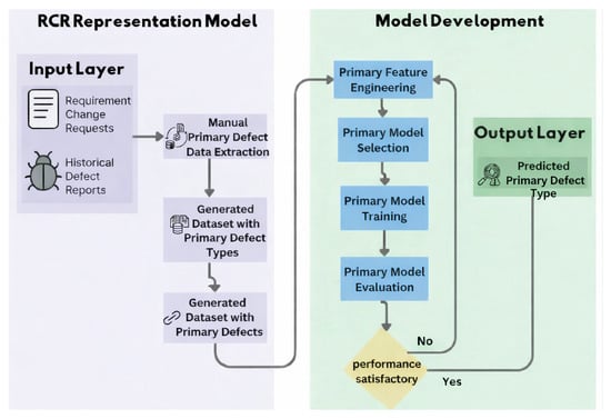
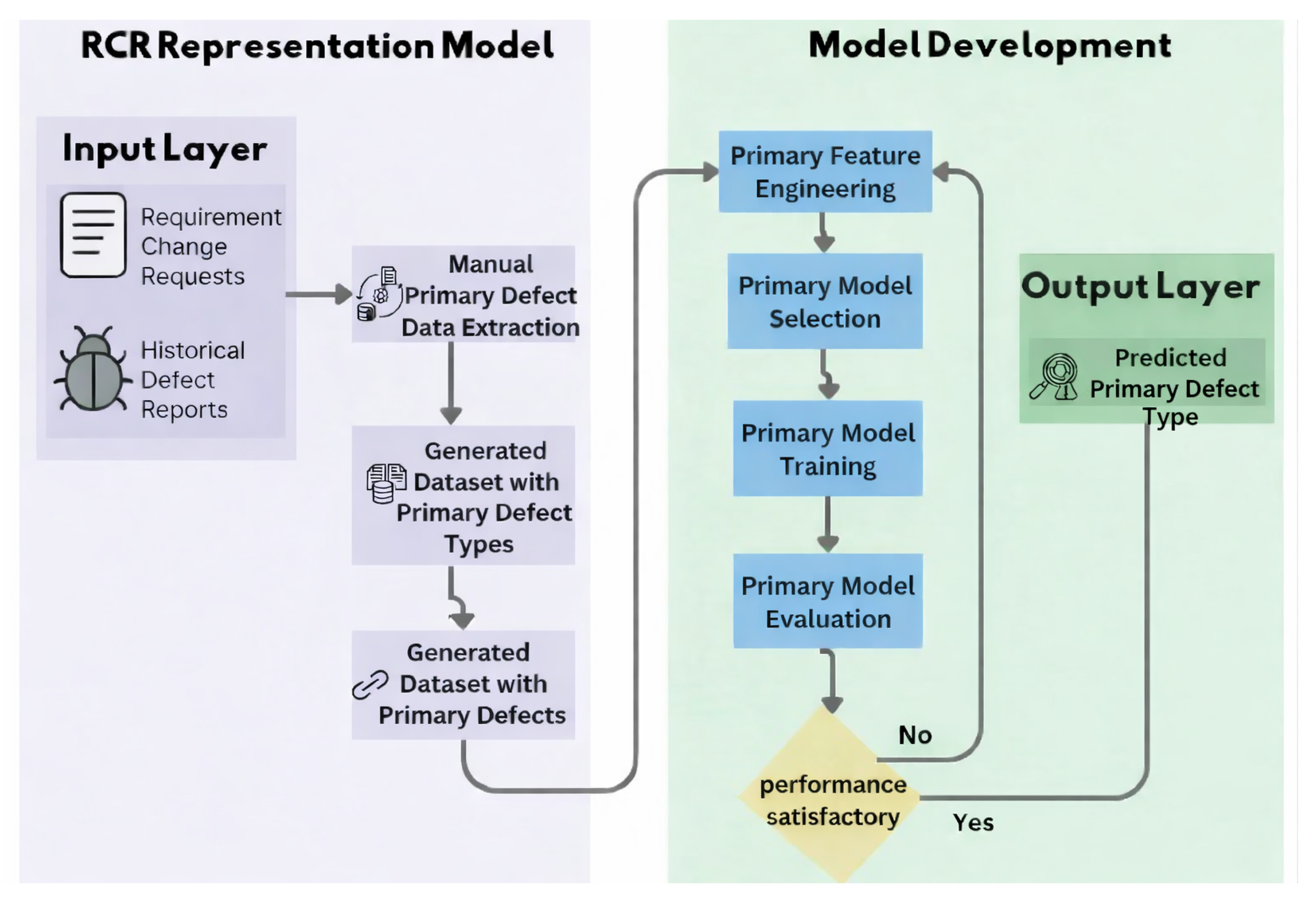
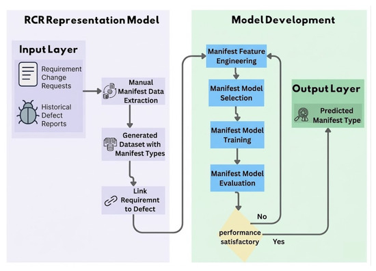
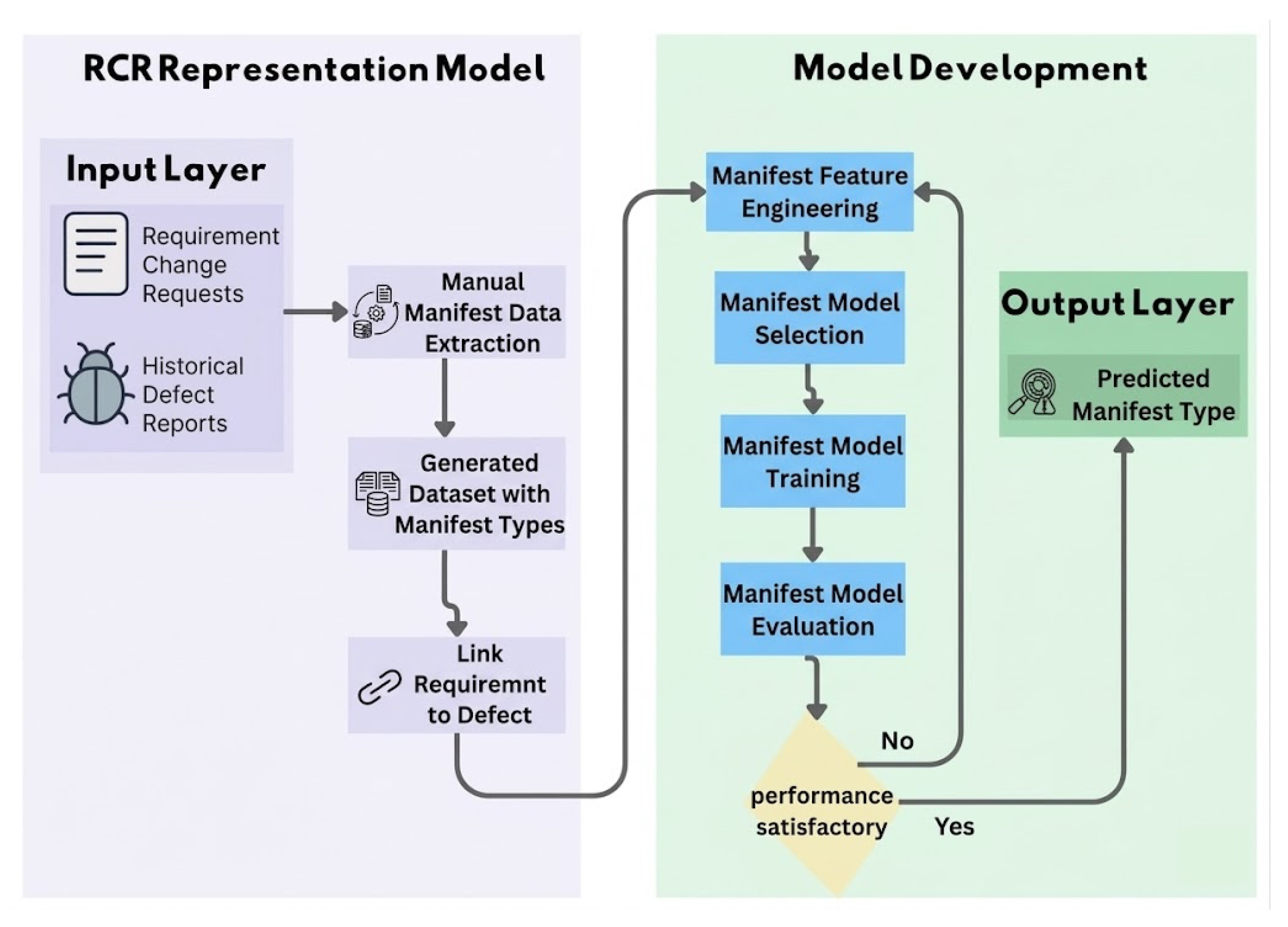

Disclaimer/Publisher’s Note: The statements, opinions and data contained in all publications are solely those of the individual author(s) and contributor(s) and not of MDPI and/or the editor(s). MDPI and/or the editor(s) disclaim responsibility for any injury to people or property resulting from any ideas, methods, instructions or products referred to in the content. |
© 2026 by the authors. Licensee MDPI, Basel, Switzerland. This article is an open access article distributed under the terms and conditions of the Creative Commons Attribution (CC BY) license.