


Abstract
Financial systems are quintessential complex adaptive systems, where stability emerges from the dynamic interactions among multiple subsystems and regulatory components. Grounded in systems theory, this study re-frames the establishment of China’s fintech regulatory sandbox as a systemic intervention within the broader financial governance framework. Utilizing this policy as a quasi-natural experiment, we employ a difference-in-differences (DID) model integrated with spatial econometric modeling to evaluate its impact on regional financial system risk—an emergent property of the system. The benchmark regression results indicate that this systemic policy innovation significantly enhances regional financial resilience, with effects that are both continuous and robust. Mechanism tests, analyzed through the lens of subsystem coordination, demonstrate that the policy curbs systemic risk by improving the synergy within economic inner cycles, outer cycles, and their dual-cycle integration, thereby optimizing the system’s internal structure and feedback loops. Further analysis reveals a significant negative spatial spillover effect, evidencing the policy’s role in reshaping inter-regional systemic linkages: it reduces financial risk in both implementing and neighboring regions, with the effect’s intensity following an inverted U-shaped pattern relative to distance. Heterogeneity analysis shows that the policy’s inhibitory effect varies significantly across different systemic configurations, including risk circulation patterns, macro–micro risk perspectives, financial inclusion coverage, government–market relationships, and the north–south regional divide. These findings provide critical insights for developing synergistic macro-prudential and micro-behavioral regulatory mechanisms, contributing to a more robust and adaptive financial security framework from a systems governance perspective.
1. Introduction
Financial systems are quintessential complex adaptive systems (CAS), where stability emerges from dynamic interactions across networks of institutions, regulators, and markets. In China, this complexity has a distinct spatial dimension, with regional financial subsystems exhibiting differentiated yet interconnected risk profiles. Safeguarding against systemic financial risks, as emphasized in national strategic directives, requires moving beyond static regulation towards adaptive governance that acknowledges this interconnectedness.
The Regulatory Sandbox, conceived by the UK’s Financial Conduct Authority (FCA) in 2015, represents a pivotal innovation in systemic governance. It functions as a bounded, safe subsystem within the broader regulatory environment, allowing for controlled testing of financial innovations. By providing a feedback-rich environment with monitored interactions between regulators and firms, it aims to balance the system’s dual needs for innovation and stability. Since 2019, China’s “FinTech Innovation Regulation Pilot” has adopted and localized this mechanism, embedding it within its national fintech development strategy. This policy shift from “passive consolidation” to “active guidance” can be viewed as a deliberate intervention in the financial system’s regulatory feedback loops, designed to learn and adapt before scaling innovations.
In response to chaos in the internet finance sector, regulators conducted specialized remediation actions to strengthen compliance during 2016–2018, establishing a foundational order for subsequent innovation. Preparatory work for the fintech pilot application, covering ten provinces and cities including Beijing and Shanghai, commenced in December 2018. In 2019, the People’s Bank of China (PBOC) issued the FinTech Development Plan (2019–2021), which first defined fintech as “technology-driven financial innovation,” clarified the sandbox’s pilot objectives, and proposed constructing an inclusive and prudent regulatory framework. This marked a policy shift from “passive consolidation” to “active guidance.” Beijing launched China’s first fintech innovation regulation pilot program in December 2019, officially initiating the Chinese version of the “regulatory sandbox”. From 2020 onward, the pilot scope expanded gradually to include cities such as Shanghai, Shenzhen, and Chongqing, incorporating more licensed financial institutions and technology companies. The FinTech Development Plan (2022–2025), issued in 2021, further proposed a “digital transformation” strategy to promote the deep integration of regulatory technology and fintech, establishing the regulatory sandbox as a key tool for implementing the “equal emphasis on security and development” principle. Its core system design achieves the dual objectives of “innovation not out of control” and “controllable risk” by limiting the testing scope and implementing dynamic risk monitoring, while also requiring test users to sign informed consent forms with clear risk compensation terms to strengthen consumer protection mechanisms. By 2025, the General Administration of Financial Supervision (GAFS) further launched the “Four Pilot Projects” to support technological innovation. These initiatives include relaxing the upper limit on merger and acquisition loan ratios for tech enterprises, extending loan terms, and promoting comprehensive reform of the intellectual property financial ecosystem in 18 pilot cities, thereby strengthening financial support for new quality productive forces like artificial intelligence and new energy. Current policy emphasizes “two-wheel drive,” promoting industrial chain integration and technological transformation through the combination of merger-acquisition finance and intellectual property finance.
Concurrently, China’s “dual-cycle” development strategy reframes the economic system’s structure, demanding that the financial subsystem enhance internal synergy while building resilience against external shocks. Existing research on regulatory sandboxes, however, predominantly examines micro-mechanisms, lacking a systemic analysis of how such a policy interacts with and reshapes the broader financial-economic system. A critical gap remains in understanding how a localized experimental policy can generate system-wide effects within the “dual-cycle” framework, influencing risk propagation and subsystem coordination across both spatial and functional dimensions.
This study aims to bridge this gap by interrogating a core systems-oriented research question: How does the fintech regulatory sandbox, as a targeted systemic intervention, reshape the emergent property of regional financial risk within China’s complex, spatially embedded financial ecosystem? We position the sandbox not merely as a policy tool but as a governance mechanism that alters the system’s internal connections, feedback processes, and boundary interactions. To investigate this, we employ the policy rollout as a quasi-natural experiment, utilizing difference-in-differences (DID) and spatial econometric models—methods well-suited for analyzing interventions in interdependent systems.
Compared to existing studies, this paper’s marginal contributions are threefold from a systems science perspective. First, it elevates the analysis from assessing a specific policy’s effect to examining a systemic intervention’s impact on an emergent property (regional financial risk), thereby contributing to the literature on complex financial system governance. Second, it introduces a multi-subsystem analytical framework (the dual-cycle perspective) to dissect the transmission mechanism. By examining how the policy enhances coordination between economic inner and outer cycles—conceptualized as interconnected subsystems—it reveals the multi-level, interactive pathways through which localized experimentation fosters system-wide resilience. Third, methodologically, it rigorously addresses the interdependence and spatial correlation inherent in complex systems, employing a suite of robustness checks and spatial econometric models to validate the causal inference and uncover the networked spillover effects of the policy.
This study diverges from conventional approaches by theorizing the regional financial environment as a Complex Adaptive System (CAS). Within this framework, financial risk is understood not as an isolated output but as an emergent property arising from the dynamic, non-linear interactions among multiple subsystems (e.g., real economy, financial institutions, regulatory bodies) and across spatial networks. The regulatory sandbox is consequently conceptualized not merely as a policy treatment but as a targeted intervention into the system’s feedback loops and connectivity structures. This ontological shift is crucial because it predicts that the intervention’s effects will manifest not only locally but also through network spillovers, and will be mediated by the system’s internal coupling.
The remainder of this paper is structured as follows: Section 2 reviews the literature through a systems lens and identifies the research gap; Section 3 establishes the theoretical systems framework and develops research hypotheses; Section 4 details the construction of system state indicators (risk measures), variable selection, and model design; Section 5 presents the empirical analysis of the policy’s direct systemic impact and robustness checks; Section 6 examines the subsystem transmission mechanisms from the dual-cycle perspective; Section 7 investigates the spatial network effects (spillovers) and heterogeneous pathways across different system configurations; and Section 8 concludes with implications for systems governance.
2. Literature Review and Theoretical Gap: A Systems Perspective
Existing scholarship on regulatory sandboxes is multifaceted, yet a cohesive analysis through the lens of systems theory—particularly regarding their role in shaping emergent systemic properties like regional financial risk—remains underdeveloped. This review synthesizes the literature along a logical continuum: from the sandbox as an adaptive governance tool, to its debated impact on financial system stability, its potential interaction with macroeconomic subsystems, and finally, the critical but underexplored dimension of spatial-systemic spillovers. This trajectory highlights the evolution from micro-institutional analysis toward a more holistic, systemic understanding, precisely where the current research gap resides.
2.1. The Regulatory Sandbox as an Adaptive Governance Mechanism
The regulatory sandbox is fundamentally an experimental governance subsystem designed to manage complexity and uncertainty in socio-technical systems. Originating in fintech [1], its application has rapidly diffused to energy [2,3], healthcare [4], and mobility [5]. This cross-sectoral adoption underscores its conceptual foundation as a controlled learning environment for regulating emerging technologies. Scholars highlight its core systemic functions: reducing regulatory uncertainty by providing a fault-tolerant space for innovation [6,7], and fostering iterative feedback loops between regulators and innovators through dynamic monitoring [8,9]. However, critiques point to inherent systemic tensions, such as challenges to legal legitimacy [10,11] and potential exacerbation of social inequities through “risk washing” [12]. A key insight from this strand is the sandbox’s role in modifying the information flows and rule sets within a specific domain, a quintessential intervention in a complex adaptive system.
Despite rich discussions on the institutional frameworks of regulatory sandboxes, rigorous empirical assessments of their macro-systemic consequences remain scarce. Emerging literature has begun to fill this gap, yet it predominantly focuses on micro-level impacts. Studies have examined firm-level outcomes, such as improved capital access and survival rates for participants, often leveraging quasi-natural experiments like staggered admission [1]. Comparative analyses further explore how different jurisdictional designs shape these micro-level results [13,14,15]. Concurrently, other work investigates the sandbox’s influence on the behavioral patterns of incumbent financial institutions [16]. Collectively, these studies provide crucial insights into sandboxes as adaptive policy subsystems that alter the behavioral rules of agents within specific national contexts.
However, while this literature has significantly advanced our understanding of sandbox adoption, design, and micro-level effects, a distinct gap persists from a complex systems science perspective. The prevailing empirical focus remains largely on structural attributes (e.g., regulatory design), agent-specific outcomes (e.g., bank behavior), or discrete policy trade-offs. What is less explored is how the sandbox, as a controlled perturbation, influences the emergent, macro-level properties of the regional financial system as a whole. Specifically, there is a scarcity of empirical studies that conceptualize and measure whether the localized, experimental learning fostered within a sandbox translates into measurable changes in system-wide resilience or vulnerability—manifested as regional financial risk—through dynamic pathways such as subsystem coupling and spatial network effects.
2.2. Conceptual Nexus: Financial Risk, Resilience, and Systemic Capacity
Within the complex adaptive systems (CAS) paradigm, it is crucial to distinguish between system state and system capacity [17]. In this study, regional financial risk, measured by our composite stress index, is conceptualized as an emergent system state reflecting the current level of dysregulation or stress within the socio-financial network.
Conversely, financial resilience refers to the system’s capacity to absorb disturbances, adapt to changing conditions, and transform if necessary while retaining its essential functions [18]. Resilience is not directly observed in calm periods but is inferred from the system’s response to shocks. The theoretical link between our measured outcome (risk reduction) and the underlying systemic property (resilience enhancement) hinges on the nature of the intervention. A standard, repressive regulatory measure might lower short-term risk at the expense of system adaptability, potentially creating latent fragility (a non-resilient outcome). In contrast, a regulatory sandbox is designed as an adaptive governance mechanism that fosters institutional learning, increases the diversity of financial solutions, and strengthens monitored interconnections [6,9]. By doing so, it augments the system’s adaptive capacity (its resilience) on multiple fronts: absorption (via better risk screening), adaptation (via iterative learning loops), and transformation (via facilitated innovation) [19].
Therefore, we posit that a sustained reduction in the systemic stress state (financial risk) induced by the sandbox is not a mere statistical correlation, but an observable manifestation of an augmented underlying capacity for resilience. The sandbox does not simply suppress risk; it cultivates a system that is inherently more capable of managing and mitigating risk endogenously. This theoretical justification underpins our interpretation of the empirical findings.
2.3. Sandbox Effects on Financial (In)Stability: A Contested Nexus
The sandbox’s impact on the financial system’s stability—a primary emergent property—is empirically contested and theoretically nuanced. One perspective, aligned with its innovation-promotion goal, finds that sandboxes improve fintech firms’ access to capital [1] and foster beneficial regulator–industry interactions [8]. Conversely, other studies caution that the relationship is not straightforward; Fung et al. (2020) find fintech innovation driven by sandboxes to be an insignificant factor for bank stability in a cross-country context [20]. This ambiguity points to the non-linear and context-dependent outcomes typical of complex systems. The potential for sandboxes to amplify systemic risks is noted in the literature, including technology dependency, data privacy breaches, and credit misallocation due to algorithmic biases. Yet, its risk-mitigation capacity is argued to stem from its design as a filtering and damping mechanism, employing access screening, real-time supervision, and polycentric governance to enhance the system’s absorptive capacity [21]. This debate reveals a literature strong on identifying micro-mechanisms and firm-level outcomes, but largely silent on how these micro-dynamics aggregate to influence meso-level, regional risk profiles.
2.4. The Macro-Systemic Context: Bridging to the “Dual-Cycle” Framework
Financial risks do not emerge in a vacuum but are co-determined by the structure and dynamics of the broader economic system. China’s “dual-cycle” development strategy explicitly frames the economy as comprising two major, interdependent functional subsystems: the domestic/internal cycle and the international/external cycle [22]. Research has begun to explore how digital technology can remove impediments within this dual-cycle framework [23], and how the strategy influences credit growth [24] and green development [25]. The internal cycle’s stability hinges on the synergistic coordination of production, distribution, circulation, and consumption, while the external cycle requires robust buffers against global shocks [26,27]. A nascent literature suggests that financial innovations and policies can optimize the coupling between these cycles. However, a critical gap exists: no study has systematically investigated whether and how a regulatory sandbox—a micro-prudential, experimental tool—can influence the functional integration and risk resilience of these macroeconomic subsystems. The theoretical linkage between a localized regulatory intervention and the macro-systemic logic of dual-cycle coordination remains unmapped.
2.5. The Spatial-Systemic Gap: Risk, Spillovers, and Network Effects
Financial systems are inherently spatial networks, where regions (nodes) are interconnected through capital, information, and expectation flows. A robust literature in spatial economics confirms that financial risks and policy effects exhibit significant spatial dependence and spillover [28,29]. Such spillovers operate through channels like policy diffusion, infrastructure externalities, and expectational cascades [30,31], which are essentially the relational pathways in a complex spatial network. While studies have examined the spatial spillovers of broader financial policies (e.g., green finance reforms), the specific network effects of regulatory sandboxes are almost entirely absent from scholarly discourse. Traditional policy evaluation, assuming regional independence, fails to capture this systemic interconnectedness. Consequently, there is no understanding of how a sandbox implemented in one region recalibrates risk not only locally but also in neighboring nodes, potentially reshaping the stability landscape of the entire regional financial network.
2.6. The Measurement of Regional Financial Risk: From Indicator Construction to Systemic State Characterization
Research on regional financial risk is predominantly dedicated to its measurement and early warning systems. These methodologies, while not always explicitly framed as such, aim to quantify the state or stress level of a complex financial-economic subsystem and can be aligned with systems thinking.
The literature evolves along three paths: (1) early warning indicator models (e.g., FR probability, STV cross-sectional regression, KLR signals, DCSD, Markov-switching) that seek to identify leading indicators of systemic phase transitions [32,33,34,35,36]; (2) econometric models (e.g., CoVaR, contingent claims analysis, distress insurance premium method) that capture non-linear and tail risks [37,38,39], providing a market-implied view of systemic vulnerability; and (3) the increasingly prevalent composite indicator method, which synthesizes multi-dimensional data into a holistic index of systemic stress, exemplified by the Financial Stress Index [40].
Among these, the composite indicator method best aligns with the systems view that a system’s state is an emergent property of interacting variables. Therefore, this study constructs a regional financial stress index, conceptualizing it as a quantifiable measure of the subsystem’s emergent “stress state”, to serve as the key dependent variable for evaluating the systemic intervention of the regulatory sandbox.
2.7. Synthesis and Identification of the Research Gap
In summary, the literature has effectively established the sandbox as an adaptive governance instrument, debated its micro-level outcomes, and developed robust methods for measuring systemic financial stress. It has separately advanced theories on macroeconomic subsystem (dual-cycle) dynamics and spatial-network interdependencies. However, these streams remain largely disconnected. The pivotal gap this study addresses lies at their intersection: a comprehensive, systems-theoretic analysis that (a) investigates the regulatory sandbox as a targeted intervention within a complex, spatially embedded financial-economic system, and (b) evaluates its efficacy using a systemic-state measure (financial stress index) that captures the emergent property of regional risk. Prior research lacks an integrated framework that connects an experimental governance tool to macro-subsystem coordination, spatial network effects, and their aggregate manifestation in regional systemic stress levels. This study aims to construct and test such a unified framework.
While our empirical analysis focuses on the regional financial stress level as the primary outcome, its significance extends to broader financial stability for two systemic reasons. First, in a networked financial system, regional stress is not isolated; it can propagate through interbank exposures, payment systems, and investor expectations, acting as a potential epicenter for systemic contagion. Therefore, a policy that demonstrably lowers regional risk directly contributes to containing systemic risk at its source. Second, and more fundamentally, the regulatory sandbox is designed not merely to suppress risk locally but to cultivate system-wide adaptive capacity. By fostering learning, innovation, and more resilient interconnections within and across regions (as evidenced by spatial spillovers), it enhances the overall system’s ability to absorb and adapt to future disturbances of any origin. Thus, evaluating its impact at the regional level provides a critical, scalable test of its potential as a macro-prudential tool for safeguarding national financial stability.
3. Theoretical Systems Framework and Research Hypotheses
Grounded in systems theory, this section reframes the regional financial environment as a complex adaptive subsystem of the national economy. Within this framework, the regulatory sandbox constitutes a controlled perturbation, and regional financial risk is the emergent property arising from nonlinear interactions across credit, investment, institutions, and policies. The following hypotheses are derived from this conceptualization.
To conclusively identify the causal effect of this staggered policy intervention, we employ a tiered empirical strategy that moves from establishing a core relationship to defending its validity against specific threats. First, our baseline multi-period Difference-in-Differences model provides the foundational estimate. We then subject this estimate to a series of rigorous, targeted challenges: the Regression Discontinuity Design tests sensitivity to timing heuristics; instrumental variables address omitted confounders; and Double Machine Learning accounts for high-dimensional, non-linear controls. Crucially, the spatial econometric model is not merely an add-on but a core component that respects the networked reality of the financial system, allowing us to distinguish local effects from global spillovers. This combination allows us to move from asking “if” the policy works, to understanding “how robustly” and “through what spatial structure” it does so.
3.1. The Sandbox as a Systemic Intervention: Impact on Financial System Resilience
The sandbox introduces new regulatory feedback loops into financial innovation. While it may initially pose systemic risks—such as technology dependency, data integrity flaws, or algorithmic misallocation—its core design functions as a filter and dampener. Through mechanisms like access screening, dynamic monitoring, and a polycentric governance structure, it reduces regulatory uncertainty, addresses information asymmetries [41], and enhances supervisory agility [42,43]. By creating a bounded, fault-tolerant space for experimentation, the sandbox strengthens the system’s absorptive and adaptive capacity. We therefore hypothesize:
H1:
The fintech innovation regulatory pilot policy enhances regional financial system resilience, thereby reducing the emergent level of regional financial risk.
3.2. Subsystem Coordination Mechanism: A Dual-Cycle Perspective
The “dual-cycle” strategy delineates two primary, interconnected functional subsystems of the economy: the inner cycle (domestic production, distribution, circulation, consumption) and the outer cycle (international trade, investment, capital flows). Financial risk often arises from dysfunctional couplings or feedback within and between these subsystems. The sandbox policy aims to improve their synergistic coordination. (1) Inner-Cycle Subsystem Optimization: The policy can rewire internal feedback loops, fostering positive dynamics between innovation and industrial upgrading, improving resource flow equity, reducing transactional friction, and stabilizing household leverage—thereby strengthening the subsystem’s internal coherence. (2) Outer-Cycle Subsystem Buffering: Its modular design acts as a controlled interface with the global system, building risk buffers at the boundary through innovations in cross-border finance and supply-chain credit. (3) Inter-Subsystem Coupling: The ultimate goal is a virtuous coupling where a resilient inner cycle provides stability and a robust outer cycle facilitates beneficial exchange, promoted by improving savings-investment matching and managing capital flow volatility.
Thus, the policy’s core mechanism lies in enhancing the functional integration and stability of these key economic subsystems.
H2:
The pilot policy enhances regional financial resilience by improving the synergistic coordination between the inner and outer economic cycles.
H2a:
It reduces risk by optimizing the production–distribution–circulation–consumption feedback network within the inner cycle.
H2b:
It mitigates risk by strengthening the investment–trade buffers and risk-filtering capacity at the outer-cycle boundary.
H2c:
It reduces risk by strengthening the overall coupling and coordination between the inner and outer cycle subsystems.
3.3. Spatial Spillover Effects: Network Reshaping in a Complex System
Financial systems are intrinsically spatial networks where regions, as interconnected nodes, transmit capital, information, and expectations—allowing risk to propagate. Traditional evaluation methods that assume independent units fail to capture this systemic interdependence. The sandbox can induce spatial spillovers by reshaping network structure and node behavior: (1) Policy Diffusion, as neighboring regions imitate the mechanism; (2) Infrastructure Externalities, where platforms developed in pilot regions create positive network effects; and (3) Expectational Cascades, whereby perceived policy success shifts risk preferences across the network. Thus, the intervention’s effects are likely to radiate through the spatial-economic network, not remain geographically isolated.
H3:
The pilot policy exerts negative spatial spillover effects on regional financial risk, reducing risk in neighboring regions through network interactions, with effect intensity decaying over network distance.
3.4. Heterogeneity Analysis: System Configuration Matters
The effect of a systemic intervention is contingent on the initial state and configuration of the target subsystem. This is evident in the heterogeneity of policy effects across different risk circulation modes. (1) Inner-cycle risks are endogenous, stemming from domestic real economy-financial system disorders. The sandbox’s “test-diffusion” mode is tailored to foster endogenous institutional innovation for such structural risks. (2) Outer-cycle risks are exogenous, characterized by cross-border network transmissions. Here, the policy’s macro-prudential “monitoring-warning” mechanism aims to build network barriers. Thus, governance effectiveness depends on matching the policy tool to the risk type, as each requires distinct damping and filtering mechanisms.
H4 (Heterogeneity of Circulation Modes):
The policy’s effectiveness differs significantly when addressing risks originating from the inner-cycle (endogenous, structural) versus the outer-cycle (exogenous, networked) subsystem.
3.5. Heterogeneity Analysis: Construction Perspectives (Macro vs. Micro)
Policy effects further exhibit heterogeneity across the hierarchical levels of the financial system. (1) Macro-level risks are systemic, involving interactions between fiscal/monetary policy and financial institutions. The sandbox addresses these through a macro-prudential “monitoring–warning–regulation” closed loop. (2) Micro-level risks are agent-specific, featuring intertwined transmissions across sectors [44,45]. Here, the policy employs RegTech for penetrating supervision and intelligent risk control. This reflects a fundamental divergence in governance logic: systemic, top–down stabilization versus precise, bottom–up management.
H5 (Heterogeneity of System Level):
The policy’s effectiveness differs significantly between macro-level (systemic) and micro-level (agent-based) risks, as they operate on distinct hierarchical levels and require different regulatory tools.
3.6. Regional Heterogeneity Analysis
Policy effects display significant geographic heterogeneity, rooted in fundamental differences in regional financial-economic ecologies—encompassing industrial structure, institutional density, and integration patterns. These ecologies constitute distinct systemic archetypes with differing vulnerabilities. For instance, northern regions often exhibit an “industry-dependent” structure with commodity-linked risk exposure, while southern regions tend toward a “market-driven” structure characterized by networked, cross-market risk transmission [46,47,48]. These divergent archetypes fundamentally shape the policy’s transmission mechanisms and efficacy.
H6 (Regional Heterogeneity):
The policy’s effect on regional financial risk differs significantly across geographic regions due to underlying differences in their financial-economic ecologies, which constitute distinct systemic archetypes.
The specific analytical framework is shown in Figure 1, which visually maps the hypothesized causal pathways within this complex system.
Figure 1.
Systems analysis framework: impact of Fintech Innovation Regulatory Pilots on regional financial risk.
4. Systems-Oriented Research Design: Operationalizing Variables and Modeling Systemic Interventions
This section translates the theoretical systems framework into an empirically testable model. We detail the operationalization of the system’s state variable (regional financial risk), the systemic intervention (regulatory sandbox), key internal coupling mechanisms (dual-cycle coordination), and the statistical model for assessing the intervention’s impact within a spatially interconnected system.
4.1. Operationalization of System Variables
4.1.1. System State Variable: Regional Financial Risk (Regrisk)
Regional financial risk is conceptualized as the emergent stress level or dysregulation state of a regional socio-financial ecosystem. It arises from the complex interactions and network dependencies among micro-financial entities. Reflecting the multi-dimensional and composite nature of systemic states, this study constructs a Regional Financial Stress Index (RFSI) based on the composite indicator method. The index synthesizes 39 indicators across six sectors (government, corporate, banking, securities, insurance, real estate), categorized into three core subsystems: Regional Macro-economy, Non-Financial Sector, and Financial Sector. Crucially, this framework integrates the dual-cycle perspective, classifying indicators as pertaining to the Domestic or International Circulation, thereby embedding the structure of the macroeconomic system into the risk measurement (see Table 1 for the complete index structure and weights).
The index is calculated using the entropy weight method, a technique suited for determining objective weights based on the informational value variation of each indicator within the system over time. The final composite value for region i is derived via linear weighting of standardized indicator values, yielding a normalized score between 0 and 1, where higher values indicate a higher system stress level. This method is also employed to calculate the regional financial stress index for 31 Chinese provinces (excluding Hong Kong, Macao, and Taiwan) from 2011 to 2022. The specific implementation steps are as follows:
(1) Standardize the 39 basic indicators within the regional financial risk index system using the range method to eliminate unit and scale differences. Distinct standardization algorithms are applied to positive, negative, and moderate indicators:
If is a moderating indicator,
where and denote the original and standardized values of the jth indicator in year i, respectively; max() and min() represent the maximum and minimum values of ; A denotes the moderate value of the jth indicator; and and represent its lower and upper boundaries.
(2) Calculate the information entropy for each indicator based on the standardized value :
where n represents the year.
(3) Based on the information entropy , the weight of each indicator is calculated:
where m represents the number of indicators.
Table 1.
Construction of regional financial stress index.
(4) The regional financial risk pressure index for each region and year is calculated using the linear weighting method, based on the standardized index value and index weight :
The value of the regional financial index ranges from 0 to 1, where higher values indicate greater regional financial risk. The results are presented in Table 2.
Table 2.
Regional financial stress index of each region.
4.1.2. Core Intervention Variable: Fintech Regulatory Sandbox Pilot (Treat × Post)
The staggered roll out of China’s Fintech Innovation Regulation Pilot is treated as a quasi-natural experiment in systemic governance. This policy represents a deliberate, controlled intervention into the regulatory–financial innovation feedback loops of selected regional systems. A difference-in-differences (DID) setup is employed: regions selected for the pilot between 2019–2022 form the treatment group (Treat = 1), while others constitute the control group (Treat = 0). The time dummy (Post) is set to 1 for all years from the onset of the pilot in each region onward.
4.1.3. Mechanism Variable: Economic Subsystem Coupling (DC)
This study extends the dual-cycle perspective, which is widely recognized by scholars for its similarity to the forms of social capital reproduction in Marxist political economy and its logical consistency with China’s specific developmental stage objectives and domestic-international context. This perspective is key to accelerating the new development pattern, which prioritizes the domestic macro-cycle while promoting mutual reinforcement between domestic and international cycles. To test H2, we operationalize the synergistic coordination between the inner (IC) and outer (OC) economic cycles—the two primary functional subsystems. We construct separate evaluation systems for IC and OC. The IC system includes 17 indicators across production, distribution, circulation, and consumption, capturing the internal flows and feedback of the domestic economy. The OC system includes 6 indicators across investment and trade, capturing the exchange and interaction with the external environment.
(1) Production: Scale is measured by the growth rate of total fixed asset investment; efficiency by the average labor productivity of the three major industries; structure by the sum of the product of each industry’s output share and its labor productivity; and innovation by the ratio of R&D expenditure to GDP.
(2) Distribution: The base is measured by total labor remuneration; the initial structure by the ratio of urban-to-rural disposable income per capita; and the redistribution structure by the ratio of social security and employment expenditures to local government general budget expenditures.
(3) Circulation: Level is measured by cargo and passenger turnover; scale by total retail sales of consumer goods and the value added of the circulation industry; and the system by per capita express delivery volume and the ratio of transportation, warehousing, and postal industry value added to GDP.
(4) Consumption: The base is measured by per capita disposable income; willingness by per capita consumption expenditure; and structure by the proportion of household equipment, transportation/communication, culture/education/recreation, healthcare, and luxury goods in total consumption expenditure, alongside the Engel coefficient.
(5) Investment: Direct inward investment is measured by actual utilized foreign direct investment (FDI); direct outward investment by non-financial outward foreign direct investment (OFDI).
(6) Trade: Import and export trade are measured by the total import and export value at the operating unit’s location, respectively; factor inflow by foreign exchange earnings from international tourism; and technology introduction by the ratio of technology introduction expenditure in large and medium-sized high-tech industrial enterprises to GDP.
- Economic Rationale for Indicator Selection and Linkage to Financial Risk
The selection of sub-indicators within the dual-cycle framework is grounded in the theory of social capital reproduction and modern macroeconomic linkages to financial stability.
- Production & Investment Indicators (e.g., fixed asset growth, productivity): Over-investment or declining productivity can signal asset bubbles or profitability crises, increasing corporate default risk—a direct precursor to systemic financial stress.
- Distribution & Income Indicators (e.g., labor share, urban–rural gap): Significant inequality can depress aggregate demand and increase social tension, making the economy more vulnerable to debt-driven booms and busts, thereby elevating financial fragility.
- Circulation & Trade Indicators (e.g., cargo turnover, export dependency): Efficient circulation supports liquidity and value realization. Conversely, trade disruptions or over-dependence can expose regions to external shocks and foreign exchange volatility, key drivers of regional financial risk.
- Consumption Indicators (e.g., disposable income, consumption structure): Household consumption is the ultimate validation of production. Stagnant income or excessive leverage for consumption can lead to household debt distress, a growing source of financial instability.
Thus, these indicators capture the fundamental health and imbalance of real economic subsystems. Deterioration in any dimension can propagate through financial linkages (credit, asset prices, expectations), ultimately manifesting as heightened regional financial risk. The dual-cycle coupling degree synthesizes these interactions, measuring the systemic coherence whose weakness is a latent source of financial vulnerability.
The development levels of IC and OC are measured using the Entropy Weight TOPSIS method. Subsequently, their coupling coordination degree (DC) is calculated using coupling models. The DC value quantifies the strength and harmony of the interaction between the two subsystems, serving as a direct measure of the macroeconomic system’s internal structural coherence, a key determinant of its overall resilience (see Table 3 for the evaluation system).
The steps of the entropy weight TOPSIS method are as follows:
(1) Determine the optimal solution and the worst solution based on the weighted matrix obtained from Equation (5):
(2) Calculate the Euclidean distances and from each evaluated object to the optimal and worst solutions:
(3) Calculate the relative proximity to the ideal solution:
where ∈ [0, 1] represents the development level of the economic “inner cycle” or “outer cycle.” A larger value of indicates a higher level of economic cycle development for the region.
Table 3.
Economic dual-cycle evaluation index system and weight calculation.
4.1.4. Control Variables: Accounting for System Configuration
To isolate the net effect of the sandbox intervention, we control for other factors that shape a regional system’s configuration and baseline susceptibility to stress (see Table 4 for the control variables). These include the system’s Digitization Level (DL), Financial Regulatory Intensity (FRI), Financial Development Level (FDL), Industrial Structure (IS), Educational Level (EL), Urbanization Level (UL), Inflation Level (IL), Innovation Capacity (INC), and Urban Construction Level (UCL). Province and year fixed effects are included to account for unobserved time-invariant systemic traits and common temporal shocks.
Table 4.
Definition of control variables.
4.2. Data Sources
This study utilizes panel data from 31 Chinese provinces spanning 2011 to 2022. Data on regional financial risk are derived from the financial stress index constructed previously. The delineation of the fintech innovation regulatory pilot is based on the Notice on Pilot Work of Fintech Application issued by the People’s Bank of China and six other ministries. Data for other control and mechanism variables were sourced from the China Statistical Yearbook, the China High-Tech Industry Statistical Yearbook, the National Bureau of Statistics (NBS) website, provincial statistical yearbooks, the CSMAR database, and the Wind database. A small number of missing values were addressed using linear interpolation.
4.3. Pilot Region Selection Mechanism and the Exogeneity Assumption
For the adoption of the sandbox to serve as a valid quasi-natural experiment, the selection of pilot regions should be uncorrelated with the future evolution of regional financial risk, conditional on observed covariates. We argue that the selection process, while not random, was based on criteria that support the “as-good-as-random” assumption for our purposes.
The selection was explicitly guided by national strategic documents, including the “FinTech Development Plan (2019–2021)” and subsequent notices from the People’s Bank of China. Official guidelines indicate that pilot regions were chosen based on a combination of factors such as: (1) existing FinTech ecosystem maturity (e.g., concentration of tech firms, digital infrastructure); (2) regional regulatory capacity and experience; (3) strategic positioning in national development plans (e.g., major city clusters, free-trade zones); and (4) willingness and preparedness of local governments to collaborate. Crucially, these criteria were forward-looking and innovation-oriented, aimed at identifying regions most capable of safely testing new technologies, rather than being a direct response to or determined by the prevailing level of regional financial system stress.
The statistically insignificant pre-treatment coefficients in our event-study analysis (Figure 2) themselves provide indirect evidence that regions selected as pilots did not have systematically different trends in financial risk prior to the intervention. Therefore, while the selection was deliberate, it was based on characteristics related to innovation capacity and governance readiness rather than the emergent stress state of the financial system we aim to explain. This supports the plausibility that the timing of the sandbox rollout is exogenous to the underlying dynamics of regional financial risk. From a systems perspective, the policy can be seen as an intervention introduced to nodes within the national financial network that were deemed to have sufficient “absorptive capacity” for experimental governance, which further mitigates concerns about reverse causality.
Figure 2.
Dynamic effects of the systemic intervention (Parallel Trend Test). Note: The plot shows the estimated yearly treatment effects () with 95% confidence intervals. The pre-treatment coefficients oscillate around zero (the horizontal solid line), while post-treatment coefficients are negative and significant.
4.4. Systemic State Descriptive
Table 5 presents descriptive statistics of the system’s state and characteristics. The Regional Financial Risk (Regrisk) has a mean of 16.325 with substantial cross-sectional and temporal variation, confirming significant heterogeneity in system stress levels. The mean of the Treat × Post variable (0.108) shows that 10.8% of observations are under the intervention. The coupling coordination degree (DC) has a mean of 0.335, indicating that for most regional systems, the inner and outer cycles are at a moderately dysfunctional coupling stage, highlighting room for systemic improvement through governance. The distributions of control variables align with known regional disparities in China’s developmental landscape.
Table 5.
Descriptive statistics of variables.
4.5. Model Design: Analyzing the Systemic Intervention Effect
This paper employs the implementation of the fintech application pilot as a quasi-natural experiment. To estimate the causal effect of the sandbox intervention on the system’s state, we employ a Two-Way Fixed Effects (TWFE) Difference-in-Differences model. Using 2019 as the policy shock year, the baseline model is specified as follows:
where i and t denote province and year, respectively; is the emergent stress level of provincial system i in year t; is a grouping dummy variable that equals 1 if province i implements the fintech innovation regulation pilot and 0 otherwise; is a time dummy variable that equals 1 for the year 2019 and onwards, and 0 otherwise; is a set of control variables affecting the regional financial risk of province i in year t; and are province and year fixed effects, controlling for inherent systemic traits and common temporal shocks, respectively; is the idiosyncratic error term. is the coefficient of interest, capturing the average change in the system’s stress level attributable to the sandbox intervention. and are parameters to be estimated.
This model provides the foundation for estimating the direct effect (H1) of the regulatory sandbox on enhancing financial system resilience. Subsequent sections will expand this model to test the subsystem coupling mechanism (H2) and the spatial network spillover effects (H3).
5. Systemic Intervention Effects: Benchmark Estimation and Robustness Verification
This section empirically tests the first core hypothesis (H1) by assessing the direct impact of the regulatory sandbox intervention on the financial system’s emergent stress level. We present the benchmark estimation, verify the validity of the quasi-experimental design, and conduct a comprehensive suite of robustness checks to ensure the estimated causal effect of the systemic intervention is reliable and not confounded by other factors.
5.1. Benchmark Estimation of the Systemic Intervention Effect
Table 6 presents the stepwise benchmark regression results. Column (1) shows the estimated effect without control variables: the coefficient for the sandbox intervention (Treat × Post) is −1.825 and statistically significant at the 1% level. This initial result indicates that the introduction of the regulatory sandbox is associated with a significant reduction in the system’s financial stress level. Subsequent columns incrementally add control variables representing different dimensions of the regional system’s configuration, such as digitization level, regulatory intensity, and economic structure. As shown in Columns (2) to (4), although the magnitude of the coefficient fluctuates, it remains consistently negative and significant at the 1% level. The fully specified model in Column (4), which accounts for the broadest set of systemic characteristics, yields a coefficient of −1.778. The estimated reduction of approximately 1.778 points in the Regional Financial Stress Index (Regrisk) is both statistically robust and economically meaningful. To contextualize this effect size, it represents roughly one-third of the sample’s standard deviation (4.96 points), indicating a substantial shift in the system’s stress state. In practical terms, this magnitude is comparable to the difference in risk levels observed between an average province and one in the top quartile of financial stability during our sample period. Consequently, the policy effect is not merely a marginal adjustment but a material enhancement of the regional system’s buffer against potential shocks. This scale of risk mitigation translates into a tangible increase in the system’s absorptive capacity, meaning that regions can withstand larger disturbances before their core financial functions are compromised. Therefore, the sandbox intervention moves the system measurably within its “safe operating space”, directly contributing to macro-financial stability.
This robust negative relationship confirms H1. The regulatory sandbox, as a designed adaptive governance mechanism, effectively enhances the resilience of the regional financial complex adaptive system, leading to a measurable decrease in its emergent stress state (regional financial risk). The stability of this result across specifications suggests the effect is not an artifact of omitted systemic confounders.
Table 6.
Impact of the Fintech Innovation Regulatory Pilot on regional financial risk (system stress level).
5.2. Validating the Quasi-Experimental Design
5.2.1. Parallel Trend Test
The credibility of the difference-in-differences design hinges on the parallel trend assumption: before the intervention, the evolutionary trajectories of the system stress level in treatment and control groups should not exhibit statistically significant differences. To test whether the pilot and non-pilot regions satisfied this assumption before the implementation of the fintech innovation regulation pilot policy, we test this by estimating a dynamic event-study model [49]:
Here, is a yearly dummy variable that equals 1 for the specific year corresponding to k and 0 otherwise. The value of k begins at −7, and its regression coefficient is omitted to avoid perfect multicollinearity. Furthermore, captures the difference in regional financial risk levels between the treatment and control groups in the corresponding year. The definitions of other variables are consistent with the benchmark model.
The results, plotted in Figure 2, show that the estimated coefficients for the pre-treatment periods are statistically indistinguishable from zero, confirming parallel trends. Crucially, in the post-treatment periods, the coefficients become significantly negative. This pattern indicates that the divergence in system stress levels is indeed a consequence of the systemic intervention, not pre-existing differential trends.
5.2.2. Placebo Tests
To rule out the possibility that the estimated effect is driven by spurious correlations or unobserved shocks, we conduct two types of placebo tests.
(1) Spatial Placebo Test. We randomly assign the “treatment group” status among all provinces 1000 times and re-estimate the model. The distribution of these placebo coefficients is centered around zero (Figure 3a). The actual estimated coefficient (−1.778) lies far in the left tail of this distribution. The associated p-values are 0.001 (two-sided) and 0.000 (left-sided), strongly rejecting the null hypothesis that our result is due to chance (Table 7). The Monte Carlo simulation of 1000 randomized trials (Figure 3b) shows the mean of the regression coefficients is near zero, with most p-values exceeding 0.1. The actual coefficient (vertical dashed line) is a clear outlier among the placebo coefficients, indicating that the baseline results are unlikely to be driven by omitted variables.
Figure 3.
(a) Distribution of spatial placebo effects for single-time-point DID. (b) Spatial placebo test for single-time-point DID. Note: Vertical dashed lines represent the estimated treatment effect of the placebo effect, and horizontal dashed lines represent a p-value of 0.1.
(2) Mixed Placebo Test. We conduct a more stringent test by randomly assigning both the treatment group status and a fake policy time for each observation over 5000 replications. As shown in Figure 4a, the actual estimate remains a clear outlier in the left tail of the resulting placebo distribution, with p-values of 0.002 (Table 7). The Monte Carlo simulation of 5000 trials (Figure 4b) confirms these results, with the mean placebo coefficient near zero and the actual estimate a clear outlier. This confirms that the mitigating effect of the fintech innovation pilot on regional financial risk is not attributable to other unobservable factors.
Figure 4.
(a) Distribution of the mixed placebo effect for single-time-point DID. (b) Mixed placebo test for single-time-point DID. Note: Vertical dashed lines represent the estimated treatment effect of the placebo effect, and horizontal dashed lines represent a p-value of 0.1.
These tests confirm that the observed reduction in system stress is uniquely linked to the actual spatio-temporal implementation of the regulatory sandbox intervention, not to other latent factors.
Table 7.
Placebo test results.
5.3. Addressing Identification in a Staggered Adoption Design
We acknowledge that the regulatory sandbox policy was implemented in a staggered manner across Chinese provinces from 2019 to 2022. In such a setting, the canonical Two-Way Fixed Effects (TWFE) estimator in Equation (11) may suffer from identification bias if treatment effects are heterogeneous across cohorts and over time (i.e., if the effect of the sandbox differs between early- and late-adopting regions or evolves dynamically after implementation). This is because the standard TWFE estimator can implicitly assign negative weights to some comparison groups, potentially contaminating the average treatment effect estimate [50,51].
To ensure the robustness of our findings against this identification concern, we adopt a two-step analytical strategy. First, we retain the conventional Two-Way Fixed Effects (TWFE) specification as our benchmark model. This serves to provide an intuitive baseline estimate and maintain continuity with the established policy evaluation literature. However, we critically augment this analysis by explicitly accounting for the staggered adoption of the regulatory sandbox from 2019 to 2022, treating it as a multi-period Difference-in-Differences (DID) design. Essential diagnostic tests, including event-study plots for parallel pre-trend inspection and the examination of dynamic treatment effects, are integral to this step. Second, and more fundamentally, we directly address the potential pitfalls of the TWFE estimator under heterogeneous treatment effects by employing modern robust estimation methods tailored for staggered rollout designs. This involves conducting diagnostic tests for the ‘negative weighting’ problem and, as our preferred specification for causal inference, applying the robust estimator proposed by Callaway and Sant’Anna (2021) or similar alternatives [52]. These methods circumvent the identification issues of TWFE by constructing valid comparisons between newly treated cohorts and not-yet-treated controls, then synthesizing cohort-specific Average Treatment Effects on the Treated (ATT) into a well-defined overall ATT. This approach not only secures the credibility of our estimated causal effect but also naturally provides an analysis of the effect’s evolution over time, aligning with a dynamic systems perspective.
5.3.1. Design of the Multi-Period Difference-in-Differences Model
Consistent with the staggered adoption framework discussed above, this study formally accounts for the phased rollout of the regulatory sandbox policy across China. Based on the timeline established by key policy documents, including the FinTech Development Plan (2019–2021) and the FinTech Development Plan (2022–2025) issued by the People’s Bank of China, pilot cities were introduced incrementally. Accordingly, we construct a treatment variable FIR (Fintech Innovation Regulation) that captures the precise timing of policy adoption for each region. For province i in year t, takes a value of 1 if the pilot policy was in effect in that region-year, and 0 otherwise.
The multi-period DID model extends the baseline specification by replacing the Treat × Post indicator with the time-varying FIR variable, while all other elements remain consistent. The model is specified as follows:
5.3.2. Results of the Multi-Period Difference-in-Differences Model
Table 8 presents the results of the multi-period DID estimation. Column (1) shows that the coefficient for the time-varying sandbox treatment indicator (FIR) is −1.729 and statistically significant at the 1% level. This indicates a significant reduction in the regional financial system’s stress level following policy adoption. The subsequent columns incrementally introduce control variables representing critical dimensions of the regional system’s configuration. As shown in Columns (2) to (4), the coefficient for FIR remains consistently negative and significant at the 1% level. The fully specified model in Column (4), which accounts for the broadest set of systemic covariates, yields a coefficient of −1.259.
Table 8.
Impact of the Fintech Innovation Regulatory Pilot on Regional Financial Risk (Multi-Period DID Specification).
This robust negative relationship, derived from a specification that accurately reflects the policy’s staggered rollout, corroborates the finding from our baseline model. It confirms that the regulatory sandbox intervention acts as an effective adaptive governance mechanism, consistently associated with a lower emergent stress state of the regional financial complex adaptive system, even after accounting for heterogeneous timing and a comprehensive set of systemic controls.
5.3.3. Parallel Trends Test for the Multi-Period DID
The validity of the staggered DID design depends on the parallel trend assumption: prior to the systemic intervention, the evolutionary trajectories of the financial stress level in eventually treated and never-treated regional systems should not exhibit statistically significant differences. We test this assumption by estimating a dynamic event-study model adapted to the staggered adoption setting:
Here, is a set of dummy variables indicating the relative time to the first treatment in region i. The coefficient captures the difference in the system’s emergent stress state between treated and control groups in period j relative to the treatment onset.
The results are plotted in Figure 5. The estimated coefficients for all pre-treatment periods are statistically indistinguishable from zero, confirming that the parallel trend assumption holds. Crucially, beginning in the treatment period, the coefficients become significantly negative. This pattern indicates that the observed divergence in system stress levels is a direct consequence of the staggered systemic intervention, not a result of pre-existing differential trends. This finding reinforces the credibility of our causal interpretation within the multi-period framework.
Figure 5.
Dynamic effects of the systemic intervention (Parallel Trend Test for the Multi-Period DID). Note: The plot shows the estimated yearly treatment effects () with 95% confidence intervals. The pre-treatment coefficients oscillate around zero (the horizontal solid line), while post-treatment coefficients are negative and significant.
5.3.4. Heterogeneous Treatment Effects in the Multi-Period DID Design
(1) Diagnostic Test for the “Negative Weights” Problem
To assess the validity of our baseline TWFE estimator under staggered treatment timing, we conduct a diagnostic decomposition following Goodman-Bacon (2021) [50]. This method decomposes the aggregate TWFE estimate into a weighted average of all possible simpler 2 × 2 DID comparisons between different treatment cohorts (early vs. late, treated vs. never-treated). The diagnosis hinges on the sign and magnitude of the weight assigned to each comparison; problematic “negative weights” can arise from comparisons between early- and late-treated units, potentially biasing the overall estimate.
The decomposition results are presented in Table 9. The majority of the weight (approximately 90%) is assigned to valid comparisons: either of treated groups against the “never-treated” cohort (weight = 0.496) or of later-treated groups against the “already-treated” cohort (weight = 0.402). Crucially, the comparison that could induce bias—using “early-treated” units as controls for later-treated ones—carries only a minimal weight (0.102). Furthermore, the average treatment effects for all three comparison types are negative and significant.
Table 9.
Goodman-Bacon Decomposition of the TWFE Estimator.
This diagnostic indicates that our baseline TWFE estimate is not driven by the problematic comparisons that lead to bias. The overall negative effect is predominantly constructed from valid comparisons within the system’s adoption dynamics, reinforcing the robustness of our initial finding that the systemic intervention significantly reduces the financial system’s stress level.
(2) Employing Robust Estimators for Heterogeneous Treatment Effects
To definitively address potential identification concerns arising from heterogeneous treatment effects in our staggered systemic intervention, we employ a suite of modern “robust” difference-in-differences estimators. These methods are specifically designed to provide credible causal inference when the effects of an intervention vary across units and time—a common characteristic of complex adaptive systems.
- Cohort-Average Estimators
We first implement the estimator proposed by Callaway and Sant’Anna (2021) (CSDID) [52]. This method avoids using already-treated units as invalid controls (“bad controls”) by calculating the Average Treatment Effect on the Treated (ATT) for each cohort-period using only not-yet-treated or never-treated units as the control group, then aggregating these into a single overall ATT. This approach aligns well with the phased nature of our policy rollout. As shown in Column (1) of Table 10, the CSDID estimate is −0.615 and remains statistically significant. This confirms that the core finding of a risk-reducing effect is not an artifact of the TWFE estimator’s limitations under heterogeneity.
Table 10.
Regression Results from Heterogeneity-Robust Estimators.
- Imputation Estimators
Next, we apply imputation-based estimators [53], which construct counterfactual outcomes for treated units using information from never- or not-yet-treated units. We employ both the Interactive Fixed Effects Counterfactual (IFEct) and the Matrix Completion (MC) estimators to account for unobserved time-varying factors. The dynamic treatment effects estimated by both methods are plotted in Figure 6. The pre-treatment effects fluctuate around zero, validating the parallel trends. Post-treatment, the ATT shows a clear and deepening negative trend, indicating that the system-stabilizing effect of the intervention strengthens over time. This pattern of dynamically evolving effects is consistent with a system undergoing adaptive learning and integration of the new governance mechanism.
Figure 6.
Dynamic Treatment Effects from Imputation Estimators.
- Stacked Regression Estimator
Finally, we employ the Stacked-DID estimator [54]. This method creates a separate dataset for each treatment cohort, matched with clean control units, and stacks them for a pooled regression with cohort-by-unit and cohort-by-time fixed effects. The result, in Column (2) of Table 10, is a significantly negative coefficient of −2.086.
The convergent evidence from this battery of robust estimators—each employing distinct identification strategies to handle effect heterogeneity—provides strong, method-agnostic support for our core conclusion. The consistent finding of a significant negative effect demonstrates that the reduction in the system’s emergent stress level (financial risk) is a robust property of the regulatory sandbox intervention, not a methodological artifact. This rigorous causal validation underscores that the policy functions as an effective adaptive governance tool, capable of enhancing the resilience of a complex, heterogeneous regional financial system.
5.3.5. Sensitivity Analysis for Parallel Trends in the Multi-Period DID
While the standard event-study analysis supports the parallel trends assumption, recent methodological advancements caution that such visual inspection may not fully capture the sensitivity of causal claims to potential, non-parallel pre-trends [55]. In complex socio-economic systems, the emergent property of financial stress can be influenced by multiple, latent factors, making it crucial to quantify how much our causal conclusion depends on the exact fulfillment of the parallel trends condition.
To formally address this, we conduct a sensitivity analysis using the “Honest DID” framework [56]. This method quantifies the robustness of our treatment effect estimates by asking: How large would a violation of parallel trends need to be to overturn our conclusion? It constructs robust confidence intervals for the treatment effect under a range of plausible deviations from exact parallel trends, parameterized by a maximum allowable post-treatment trend difference (Mbar). We set Mbar based on the estimated standard errors of the pre-treatment coefficients, following Biasi and Sarsons (2021) [57].
The results are presented in Figure 7. The panels (a) through (d) show the robust confidence intervals for the treatment effect in the implementation year and the three subsequent years, under varying degrees of allowed post-treatment trend divergence. Critically, even under the most conservative deviation considered, the 95% robust confidence intervals for the systemic intervention’s effect do not include zero in any post-treatment period.
Figure 7.
Sensitivity of Treatment Effects to Violations of Parallel Trends (Honest DID). Note: The red vertical solid line represents the scenario where the policy treatment effect does not deviate, i.e., the initial state.
This analysis demonstrates that the observed reduction in the system’s stress level is not a fragile inference reliant on an implausibly perfect pre-trend. The causal claim that the regulatory sandbox enhances systemic resilience is robust to reasonable concerns about pre-existing differential trends. This finding significantly strengthens the credibility of our identification strategy within the complex, real-world context of a gradually diffusing policy across a heterogeneous system of regions.
Methodologically, our application of robust staggered DID estimators contributes to the literature by demonstrating how to conduct credible policy evaluation within complex, real-world settings where interventions are rolled out gradually across a system’s components—a common scenario in systems-oriented governance.
5.4. Addressing Endogeneity: A Multi-Method Approach
While the quasi-experimental design and placebo tests provide strong evidence, we employ multiple advanced econometric strategies to further address potential endogeneity, thereby aligning with rigorous systems science methodology that demands robust causal inference.
5.4.1. Propensity Score Matching DID (PSM-DID)
Although the benchmark regression controls for a series of regional characteristics and considers factors such as economic development level and financial innovation, alongside passing parallel trend and placebo tests, endogeneity may persist. This could arise if pilot regions were preferentially selected from more economically developed urban areas, potentially biasing the difference-in-differences (DID) results. To mitigate this endogeneity concern, we first employ propensity score matching (PSM). Specifically, we use the baseline model’s control variables to predict the probability of a region becoming a pilot (via Logit estimation). We then apply 1:20 nearest-neighbor, caliper, and kernel matching methods to identify suitable control groups for the treatment samples, retaining only those control groups that show no significant pre-policy differences from the treatment group. Finally, we re-estimate the DID model on this matched sample. Figure 8 presents the matching balance test, displaying characteristic differences between pilot and non-pilot regions before and after the three matching methods. Post-matching, the characteristics between groups are substantially balanced, and the standardized biases of variables are significantly reduced, indicating the PSM procedure successfully ensures comparability. Table 11, Columns (1)–(3), reports the regression results for the three matching methods. The coefficients for Treat × Post remain significantly negative at the 1% level, consistent with the benchmark results, confirming their robustness.
Figure 8.
Comparison of differences between treatment and control groups before and after PSM.
Table 11.
Results of PSM-DID endogeneity test.
5.4.2. Regression Discontinuity Design (RDD)
Using the policy inception year (2019) as a cutoff, we test for a discontinuity in the system stress level timeline. We test for a discontinuity in regional financial risk around this point by estimating the following model:
where is the running variable, representing the year interval from the current time to the 2019 policy cutoff in region i. is the treatment dummy, equaling 1 for periods from 2019 onward. The coefficient captures the discontinuity in regional financial risk at the policy cutoff. The function represents the polynomial functional form of the running variable and its interaction with ; a linear setting uses a first-order interaction, while a quadratic setting includes a second-order term. This paper uses nonparametric estimation for the RDD. The optimal bandwidth is selected by minimizing the mean squared error at the cutoff point following the Imbens and Kalyanaraman (2012) IK method [58], which yields an optimal bandwidth of 3. Estimations are conducted using this optimal bandwidth, as well as 0.5 and 2 times this value.
The results are presented in Table 12. Under the optimal bandwidth (Columns 3–4), the coefficients for the grouping variable are significantly negative after controlling for first- and second-order interaction terms, indicating a significant reduction in regional financial risk following the policy implementation. The results using 0.5x and 2x the optimal bandwidth (Columns 1–2, 5–6) also show significantly negative coefficients, reaffirming the robustness of the benchmark findings.
Table 12.
Endogeneity test results of the regression discontinuity model.
5.4.3. Instrumental Variable (IV) Estimation
To address potential endogeneity from omitted variables, reverse causality, and measurement error, this paper employs an instrumental variable approach. A valid instrument must satisfy relevance and exclusion restrictions. We use the one-period lag of the explanatory variable (Treat × Post) and the number of FinTech firms (Company) as instruments for the fintech innovation pilot policy, conducting two-stage least squares (2SLS) estimation.
Table 13 reports the IV regression results. Columns (1) and (3) present the first-stage results, showing that both instruments (IV1_L.Treat × Post and IV2_Company) are significantly correlated with the pilot policy. The first-stage F-statistics (Kleibergen–Paap Wald F) exceed the Stock–Yogo critical value at the 10% level, rejecting the hypothesis of weak instruments. The Kleibergen–Paap LM statistics significantly reject the null of underidentification at the 1% level, confirming instrument validity. Columns (2) and (4) show the second-stage results: the coefficients for Treat × Post remain significantly negative at the 1% level, indicating that fintech innovation regulation reduces regional financial risk, thus reaffirming the benchmark conclusion’s robustness.
Table 13.
Endogeneity test results of instrumental variable approach.
5.4.4. Double Machine Learning (DML)
To handle high-dimensional controls and potential non-linearities among system configuration variables, we employ a double machine learning (DML) approach, specifying the following partially linear model:
where is the target treatment effect coefficient; is an error term with conditional mean zero; is a vector of high-dimensional control variables; and g() is a nonparametric function estimated via machine learning. The treatment effect estimator is:
To ensure unbiased estimates in finite samples, we construct an auxiliary regression:
where m() is the conditional expectation of the treatment, estimated via machine learning, and is the error term. The procedure involves: (1) estimating and obtaining residuals = ; (2) estimating the main regression = () + ; and (3) using as an instrument for to obtain the unbiased estimator:
Table 14 presents the DML estimates of the policy effect, using a 1:4 sample split and four algorithms: Lasso Regression, Ridge Regression, Elastic Net Regression, and Neural Network Regression. Whether controlling for linear or quadratic terms, the coefficients for the fintech innovation pilot remain significantly negative at the 1% level across all models, robustly verifying that the policy inhibits regional financial risk.
Table 14.
Endogeneity test results of the four models under the double machine learning method.
5.4.5. Controlling for Concurrent Interventions and Trends
Concurrent policies during the sample period may confound the estimated effect of the fintech pilot. To address this, we control for five potentially interfering policies: the “Broadband China” strategy, the “Belt and Road” initiative, the Yangtze River Economic Belt policy, the E-commerce Model City policy, and the Comprehensive Cross-border E-commerce Pilot Zone. Table 15 reports the results. Columns (1)–(5) control for each policy individually, while column (6) controls for all five simultaneously. The pilot policy’s coefficient remains significantly negative at the 1% level in all specifications, confirming that our core findings are robust to the influence of other policies.
Table 15.
Endogeneity test results excluding other interfering policies.
5.4.6. Introduction of Time Trend Terms
To control for heterogeneous time trends in regional financial risk and mitigate bias from interregional risk transfer, we introduce province-specific linear time trends into Equation (11). The results, presented in Table 16, show the treatment effect remains significantly negative at the 1% level, consistent with the benchmark regression. This largely rules out bias from divergent regional development paths and further corroborates the inhibitory effect of fintech innovation regulation on financial risk.
Table 16.
Endogeneity test results with the introduction of time trend terms.
5.5. Other Robustness Tests
5.5.1. Replacement of the Explanatory Variable’s Measurement Method
To ensure our results are not driven by the weighting scheme of the financial risk index, we re-measure the explained variable using the CRITIC method to determine indicator weights. The regression results using this new measure (Table 17, Column 1) align with the benchmark results, indicating that the risk-mitigating effect is robust to alternative measurement approaches.
Table 17.
Results of other robustness tests.
5.5.2. Changing the Clustering Method
To address potential bias from unobservable time-varying confounders and limited clusters, we adopt more conservative inference techniques. We cluster standard errors at the province level and use the Wild Cluster Bootstrap method to account for heteroskedasticity and few clusters. The result (Table 17, Column 2) remains significantly negative, confirming robustness.
5.5.3. Changing the Time Window
To alleviate concern that the long pre-treatment period (2011–2018) may bias the results, we restrict the sample to 2015–2022. The result (Table 17, Column 3) remains unchanged, demonstrating that our findings are not sensitive to the chosen time window.
5.5.4. Excluding Municipalities
Direct-controlled municipalities (Beijing, Shanghai, Tianjin, Chongqing) possess unique economic advantages that could independently influence financial risk. To rule out selectivity bias, we exclude these municipalities. The result (Table 17, Column 4) remains significantly negative, indicating the policy effect is not driven by these outlier regions.
5.5.5. Lagged Control Variables
To mitigate potential reverse causality, we lag all control variables by one period. The result (Table 17, Column 5) remains significantly negative at the 1% level, reinforcing the robustness of our conclusions.
5.5.6. Two-Period Difference-in-Differences Model
To test the policy’s sustained effect and rule out model specification bias, we construct a two-period DID model. We average variables over the pre-policy (2011–2018) and post-policy (2019–2022) periods and re-estimate the model. The results (Table 17, Column 6) remain significantly negative, confirming that the policy effect is persistent and robust to alternative model specifications.
6. Mechanism Analysis: Pathways of Systemic Intervention in Subsystem Coupling
The previous section robustly established the direct, system-stabilizing effect of the regulatory sandbox intervention. This section delves into the internal “black box” of the complex system to uncover how this intervention achieves its effect. Grounded in the dual-cycle framework, we analyze the transmission pathways by examining the intervention’s impact on the functional performance of key economic subsystems (inner and outer cycles) and, crucially, on the synergistic coupling and coordination between them. This mechanistic analysis tests Hypothesis 2 and its sub-hypotheses, moving from correlation to an understanding of systemic causal pathways. It also explores the spatial evolution characteristics of the coordinated development of the dual cycle across Chinese provinces, classifying them using the natural breakpoint method and hotspot analysis.
6.1. Subsystem Performance and Inter-Subsystem Synergy: Testing the Transmission Pathways
To dissect the mechanism, we first quantify the state of the subsystems. The development levels of the Inner Cycle (IC) and Outer Cycle (OC) are measured using the Entropy Weight TOPSIS method. Their interaction and synergy are then captured through coupling models, calculating the coupling degree and the comprehensive coupling coordination degree (denoted as DC), which serves as a holistic measure of systemic synergy. We employ a coupling degree model and a coupling coordination degree model to measure the level of economic dual-cycle development:
where a and b denote the inner cycle subsystem and outer cycle subsystem, respectively. denotes the coupling value between the two subsystems, ranging from 0 to 1. denotes the comprehensive evaluation index. α and β are weighting coefficients that satisfy α + β = 1; here, α is set to 0.7 and β to 0.3. denotes the coupling coordination degree, which lies between 0 and 1. The following model is adopted to test the mechanism:
where represents the mechanism variables: the performance of individual links within IC and OC, their interaction terms, and the overall DC index. Other variables are consistent with the baseline model.
6.1.1. Enhancing the Inner Cycle Subsystem (IC)
The regulatory sandbox, by creating a controlled environment for financial innovation, optimizes resource flows and feedback loops within the domestic economic subsystem. (1) Production: It improves capital allocation, fostering a positive feedback loop between innovation investment and industrial chain resilience. (2) Distribution: It promotes inclusive digital finance, improving income distribution structure and reducing inequality-driven systemic risks. (3) Circulation: It enhances payment system efficiency, lowering transactional friction and systemic vulnerability. (4) Consumption: It stimulates new consumption models and refines credit risk management, bolstering market stability. Table 18 (Columns 1–4) shows the significant positive coefficients across all four inner-cycle links (Production, Distribution, Circulation, Consumption) indicate that the sandbox policy systematically enhances the functional efficiency of the domestic economic subsystem. This validates H2a, indicating the policy reduces financial stress by optimizing internal subsystem efficiency and stability. Beyond merely reducing transactional frictions and default probabilities (risk mitigation), this integrated optimization fundamentally augments the system’s “absorptive capacity” [17]. Specifically, it enables the regional financial system to maintain critical capital and payment flows during periods of stress, thereby preserving its core functions against disturbances.
Table 18.
The impact of the Pilot Policies of Fintech Innovation and Regulation on the links in the economic inner cycle and outer cycle.
6.1.2. Fortifying the Outer Cycle Subsystem (OC)
Through its “modular regulation” approach, the sandbox helps manage cross-border financial innovation risks. (1) Investment: It facilitates digital cross-border assets and optimizes portfolios, mitigating exchange rate risks. (2) Trade: It innovates supply chain finance models, allowing for precise assessment and mitigation of trade-related financial risks. Table 18 (Columns 5–6) confirms the policy’s positive effect on both investment and trade links, supporting H2b. This demonstrates the policy’s role in strengthening the system’s boundary buffers against external shocks. The facilitation of investment and trade links demonstrates the policy’s role in building buffers at the system’s boundary. This ‘modularized regulation’ does more than isolate cross-border risks; it actively fosters the system’s ‘adaptive capacity’. By diversifying financing channels and introducing innovative hedging tools, the system gains a greater repertoire of responses to reconfigure resources in the face of external shocks, such as sudden capital flow reversals or global market volatility.
6.1.3. Fostering Synergistic Interactions Between Subsystems
The above analysis details the impact of the regulatory pilot on regional financial risk through individual links of each cycle. However, as an integrated economic system, these links do not exist in isolation. It is essential to strengthen their organic combination and cyclic connection to form a higher-level dynamic equilibrium system. The system’s resilience stems not only from strong subsystems but from their effective coupling. The policy enhances synergistic interactions within and across cycles.
Table 19 presents the results for the two-by-two interaction terms representing synergies within the economic cycle. In both Panel A and Panel B, the regression coefficients for these interaction terms are significantly positive at the 1% level. This indicates that by deeply reconfiguring and accelerating the interaction mechanisms of key links, the pilot policy better stimulates the synergistic effect between the inner and outer cycles, forming a “two-wheel drive” for financial risk mitigation. Thus, Hypothesis 2c is supported. The enhancement of coupling coordination between and within cycles is perhaps the most salient evidence of resilience-building. Stronger synergy, such as the real-time feedback between consumption and production, creates a “learning and self-adjustment capability” within the system [19]. This moves governance beyond static buffering towards dynamic stewardship, where the system itself can better anticipate disruptions, learn from incremental feedback, and reorganize without losing its fundamental identity.
Within the inner cycle dimension, the pilot strengthens the coupling between production and distribution, reducing the risks of inventory backlog and overcapacity by establishing a market-based factor allocation mechanism. Simultaneously, it promotes the digital integration of consumption and distribution, enabling real-time feedback from consumption data to the production side, which improves market responsiveness and reduces liquidity risk. In the outer cycle dimension, the pilot optimizes the linkage between investment and trade, promoting a two-way balance through innovations in cross-border investment tools and the establishment of an international trade single window, effectively diversifying investment risks. In summary, the pilot policy constructs a regional financial risk “firewall” by reshaping the interaction mechanisms of the four major links and stimulating multi-level synergistic effects.
Table 19.
Impact of the Pilot Regulatory Policies on Financial Technology Innovation on the interaction of various links in the economic subsystem cycle.
6.1.4. Strengthening Overall Systemic Coupling (DC)
The analysis of the economic inner and outer cycles confirms their facilitatory role in reducing regional financial risk. A comprehensive analysis of the subsystems (IC and EC) and the overall dual cycle (DC) target layer shows that the regression coefficients for IC, OC, and DC are significantly positive at the 1% level in both single-period and multi-period models (Table 20). This indicates that by enhancing the resilience of each economic subsystem, the policy reduces regional financial risks, thus validating Hypothesis 2.
Table 20.
Impact of Pilot Policies on Financial Technology Innovation Regulation on the economic inner cycle, the economic outer cycle and the dual cycle of the economy.
In summary, at the inner cycle level, the pilot enhances capital flow efficiency and market transparency, reduces financing costs, and strengthens the endogenous stability of the real economy by optimizing payment systems and promoting supply-chain finance innovation. At the outer cycle level, it improves cross-border capital flow monitoring and innovates foreign exchange risk management tools. In the dual-cycle linkage dimension, the pilot promotes efficient allocation of internal and external resources by building integrated financial infrastructures, enhancing the risk-hedging ability of market players and forming a dual protection mechanism.
Overall, the pilot policy constructs a financial governance framework aligned with the dual-cycle pattern. It systematically enhances the resilience of the regional financial system from three dimensions—market infrastructure, policy tools, and risk isolation mechanisms—forming a positive cycle of “enhanced risk controllability → stabilized market expectations → stabilized capital flows” and ultimately achieving a fundamental reduction in regional financial risks.
6.1.5. Theoretical Synthesis: From Risk Mitigation Pathways to Systemic Resilience Building
Our empirical journey from measuring risk reduction to inferring resilience enhancement is substantiated by the specific pathways through which the sandbox operates. The mechanisms we identified—subsystem optimization, inter-subsystem coupling, and positive network spillovers—are not hallmarks of risk suppression but are classic levers for building resilience in complex systems [59]. The reduction in regional financial risk observed here is therefore best interpreted as the equilibrium outcome of a system whose intrinsic capacity to handle volatility, uncertainty, and shock has been structurally enhanced. This distinction is critical for policy: it shifts the goal from achieving static stability to fostering dynamic, learning-based resilience.
6.1.6. On Establishing Causal Linkages for the Mechanisms
We acknowledge that establishing causal mediation—proving that the policy causes the outcome through the specified subsystems—requires more than documenting correlations. Our goal in this section is to present evidence consistent with such a causal chain, while transparently discussing its identification challenges and bolstering our case with robustness checks.
To strengthen the causal interpretation, we go beyond simple association. First, we examine the timing and dynamics of the effect: the improvement in dual-cycle coupling (Figure 9) follows, rather than precedes, the policy implementation. Second, we draw on the richness of our heterogeneity analysis: the finding that the policy effect is stronger in regions with certain initial system configurations (e.g., lower financial inclusion) provides a form of conditional evidence that is harder to explain by pure coincidence.
Figure 9.
Thermal map of economic dual-cycle level in Chinese provinces and regions from 2011 to 2022.
Furthermore, to address the concern that the mechanism variables might be endogenous, we consider alternative pathway tests. For instance, we test whether the policy’s effect on financial risk is mediated by the improvement in a particular subsystem’s performance, after controlling for other potential channels.
6.2. Spatial Heterogeneity in Systemic Synergy: An Evolutionary Perspective
The mechanism’s effectiveness is conditioned by the initial state and spatial configuration of the regional systems. We analyze the spatial evolution of the DC index (2011–2022) to contextualize the findings. Figure 9 (Heat Map) and Figure 10 (Spatial Distribution) reveal a persistent, gradient pattern of “strong in the east, weak in the west; strong on the coast, weak inland.” This spatial heterogeneity reflects deep-seated differences in systemic endowments.
Figure 10.
Spatial distribution of the level of coordinated development of the dual-cycle in Chinese provinces.
Figure 9 shows the economic dual-cycle (DC) levels across Chinese provinces from 2011 to 2022. The DC levels in most provinces show steady improvement, with the national average climbing from 0.2846 in 2011 to 0.39 in 2022. However, regional development imbalances remain prominent. Eastern coastal provinces continue to lead, with Zhejiang, Jiangsu, Guangdong, Beijing, and Shanghai exceeding 0.5 by 2022; Guangdong reached a peak of 0.8594.
The central region’s development level is generally stable above the national baseline, while the western region lags behind, forming a three-tiered gradient development pattern. This disparity may be attributed to theoretical constraints in the western region, including lagging infrastructure, an imbalanced industrial structure, talent and technology bottlenecks, differences in policy implementation, and ecological and geographical constraints. Lagging infrastructure weakens factor flow efficiency, while an over-reliance on resource-based industries inhibits participation in high-value-added global chains. Talent loss and insufficient innovation capacity further hinder development. These constraints are intertwined, leading to the western region’s relative weakness in the dual-cycle pattern.
To better visualize the spatial distribution characteristics of the coordinated development of the dual cycle, we classified the coordination level into five types using the natural breakpoint method: well-coordinated, basically coordinated, on the verge of imbalance, mildly unbalanced, and seriously unbalanced. Figure 10, generated with Arcmap10.8 software, depicts the spatial distribution in 2011, 2016, and 2022.The overall pattern shows a gradient of “strong in the east and weak in the west, strong on the coast and weak inland.” The eastern region, as the core engine, benefits from advanced infrastructure, a diversified industrial structure, and a high degree of openness, forming a high-level agglomeration for the dual cycle. The central region, with its transportation hubs and domestic demand potential, serves as a transition zone for industrial transfer, though its industrial chain resilience needs strengthening. The western region, constrained by the factors mentioned above, lags behind, showing a three-tier differentiation pattern. The spatiotemporal evolution shows that in 2011, only Beijing, Shanghai, Jiangsu, and Guangdong had reached a well-coordinated level, reflecting the core hub status of the Yangtze River Delta and Pearl River Delta. By 2016, with the deepening of openness, Zhejiang and Shandong were promoted to well-coordinated regions, and the central provinces improved significantly. By 2022, amid a complex international environment, the national coordination level improved steadily, but regional differentiation became more significant. Fluctuations in provinces like Jilin and Hubei reflect both the resilience of the dual-cycle pattern and the ongoing structural challenges in regional coordination, highlighting the need for improved institutional supply.
7. Spatial Network Effects and Systemic Resilience Under Heterogeneous Configurations
The preceding analysis confirms the regulatory sandbox as a direct and effective intervention for enhancing the internal coupling and stability of regional financial-economic systems. This section extends the inquiry to the networked dimension of complex systems, examining how the intervention’s effects propagate across spatial connections (H3) and how its efficacy is moderated by the heterogeneous initial configurations of regional subsystems (H4, H5, H6). This provides a holistic view of the policy’s role in reshaping the inter-regional risk network.
7.1. Spatial Network Effects: Reshaping the Inter-Regional Risk Contagion Network
Financial systems are intrinsically spatial networks, where regions (nodes) are interconnected. The standard DID model in Equation (11) provides a robust estimate of the average direct effect of the regulatory sandbox, under the assumption that regions (system units) are independent. However, this assumption is fundamentally at odds with our core theoretical proposition that the financial system is a spatially embedded complex network. Financial risks, capital flows, and policy signals propagate through interconnected nodes (regions), creating spillovers and feedback loops. To empirically honor this systemic reality and test Hypothesis 3, we must employ a model that explicitly incorporates this interdependence. Therefore, we adopt a Spatial Durbin Difference-in-Differences (SDM-DID) model as our primary specification for assessing the policy’s total systemic impact. The SDM-DID model, specified in Equation (27), incorporates a spatial weight matrix, W, which formally represents the structure of connections within the regional network. This allows us to decompose the total effect of the sandbox intervention into two distinct components: (1) the direct effect, capturing the change within the treated region itself, and (2) the indirect (or spillover) effect, capturing the impact propagated to and from its connected neighbors through the network. This decomposition is not merely a statistical refinement; it is the direct empirical operationalization of the systems science tenet that the state of any unit is co-determined by its own attributes and its linkages to others. The magnitude and significance of the indirect effect will provide a quantitative measure of the policy’s network-wide resilience-enhancing capacity.
For the spatial weight matrix, we first consider that risk transmission may be jointly affected by geographic and economic distance. We construct an economic-geographical weight matrix . For i ≠ j, and ; for i = j, . Here, is the inverse of the absolute difference in per capita GDP between provinces i and j, and is the inverse of the squared latitude-longitude distance between provincial geographic centers. Both and are normalized. Second, to capture spillover effects under different spatial linkages and test the robustness of the results, we construct a spatial economic distance matrix . For i ≠ j, ; for i = j, . This paper employs the SDM-DID model with both the economic-geographical and spatial economic distance weight matrices, specified as follows:
where is the constant term, is the coefficient of the spatial lag term for regional financial risk, is the coefficient of the spatial lag term for the pilot policy, represents the coefficients for the spatial lag terms of the control variables, is the spatial weight matrix, and denotes individual fixed effects. Other variables are consistent with the baseline model.
7.1.1. Validating the Networked Structure and Model
We first confirm the presence of spatial autocorrelation, a statistical signature of networked interdependence, in regional financial risk. Table 21 shows Moran’s I indices are significantly positive across all years for both an economic-geographic nested matrix and a pure economic distance matrix, justifying spatial econometric analysis.
We further test if the Spatial Durbin Model (SDM) can be simplified to a Spatial Lag Model (SAR) or Spatial Error Model (SEM); results are in Table 22. First, the Lagrange Multiplier (LM) and robust LM statistics for both the SAR and SEM are significant at least at the 5% level, indicating the presence of spatial lag and error terms, thus initially supporting the SDM. Second, both the LR and Wald tests significantly reject the null hypothesis that the SDM can be simplified to SAR or SEM. Therefore, the SDM is more appropriate. The Hausman test also significantly rejects its null hypothesis at the 1% level, leading us to select the two-way fixed effects SDM model.
Table 21.
Global Moran’s Index of regional financial risk.
Table 22.
Reasonability test of spatial econometric model.
7.1.2. Analysis of Spatial Network Effect Test Results
Based on the above evidence, we control for individual and year fixed effects and estimate Equation (27) under both weight matrices. The results in Table 23 show that the coefficients for Treat × Post and other spatial lag terms are significantly negative for both matrices. This indicates that the fintech innovation regulation pilot has a significant negative spatial spillover effect on regional financial risk, reducing risk in both implementing and neighboring regions, thus supporting Hypothesis 3. The positive and significant spatial lag term coefficient (rho) for regional financial risk confirms that a region’s financial risk is closely related to that of its neighbors.
Table 23.
Spatial network effect regression results and decomposition results of direct and indirect effects.
7.1.3. Decomposition Results of Direct and Indirect Effects
The SDM coefficients do not directly represent marginal effects; thus, we decompose the spatial effects into direct, indirect, and total effects. The decomposition results in Table 23 reveal a significantly negative indirect effect, which is economically substantial and, in some specifications, exceeds the direct effect. This finding provides compelling empirical validation of the regional financial system’s networked nature. It demonstrates that the regulatory sandbox intervention does not operate in isolation; its stabilizing influence ripples through the socioeconomic network, enhancing resilience in neighboring regions. The total systemic benefit (the sum of direct and indirect effects) is therefore significantly greater than what a traditional, non-spatial model would estimate, highlighting the risk of underestimating policy impact when systemic interconnectedness is ignored.
7.1.4. Ruling out Alternative Explanations for Spatial Correlation
While our spatial econometric model identifies a pattern consistent with policy spillovers, we carefully consider two alternative explanations for the observed inter-regional correlation: common shocks and structural co-movement.
(1) First, our model includes year fixed effects, which non-parametrically absorb any nationwide common shocks (e.g., broad monetary policy changes, global financial cycles) that could simultaneously affect all regions’ financial stress levels in a given year.
(2) Second, the non-linear, distance-decaying pattern of the spillover effect (Figure 11) is difficult to reconcile with pure structural co-movement. If correlation stemmed solely from similar economic structures (e.g., two resource-dependent provinces reacting to the same commodity price shock), we would not expect the effect strength to systematically weaken with geographic distance. The fact that the effect is strongest within a ~250 km radius is more indicative of policy and information diffusion through spatially bounded networks—a hallmark of genuine spillovers.
Figure 11.
Spatial spillover effects of Fintech Innovation Regulatory Pilots.
(3) Therefore, while we cannot definitively rule out all forms of latent co-movement, the combination of stringent time controls and the distinctive spatial pattern of the effect support our interpretation that the observed negative correlation is primarily driven by the network-transmitted impact of the regulatory sandbox intervention.
7.2. The Spatial Boundary of Network Effects
7.2.1. Model Construction of Radiation Range
The previous analysis confirms the existence of a spatial spillover effect from the fintech innovation regulation pilot policy. According to the theories of spatial economics and financial geography, this spillover effect not only diminishes with increasing distance but also has a spatial boundary, leading to a more pronounced effect within a certain range. To further explore the radiation range of this policy’s spillover effect, we establish the following model:
Equation (28) introduces a new set of dummy variables based on Equation (11). The parameter d denotes the spherical distance (in kilometers, d ≥ 100) between a non-pilot province and the nearest pilot province. Specifically, = 1 if there is a pilot province within the spatial range of (d-50, d] kilometers from province i in year t, and 0 otherwise. The coefficient in Equation (28) represents the impact of the pilot policy on the regional financial risk of a neighboring region at distance d. We analyze the regression results of Equation (28) for d = 100, 150, 200, ⋯⋯ 700 in 50 km increments to test the spatial decay characteristics and the radiation scope of the policy effect by comparing the economic and statistical significance of at different thresholds.
7.2.2. Analysis of the Result
Figure 11 plots the trend of the coefficient with spatial distance based on the regression results of Equation (28) (with a 99% confidence interval). The effect of the pilot policy on regional financial risk in neighboring provinces follows an “∽” shape, first rising, then falling, then rising again, and finally falling. The coefficient estimates are significantly negative in the 100–150 km and 200–250 km ranges, indicating that the spatial spillover effect gradually increases with distance within these intervals. However, the coefficients become statistically insignificant when the distance threshold exceeds 250 km or falls within the 150–200 km range. This suggests that the effective boundary of the spatial spillover effect is 250 km.
The nonlinear decay pattern of the spillover effect, strengthening within a certain range before dissipating beyond approximately 250 km, offers a nuanced view of the system’s functional connectivity structure. It suggests that the policy’s stabilizing signals are strongest within a defined ‘systemic neighborhood’ characterized by intense economic and informational exchange. The initial increase may reflect the overcoming of immediate competitive ‘shadow effects,’ while the eventual decay marks the boundary of effective network influence. This pattern aligns with complex network theory, where influence propagation is often non-linear and constrained by connection strength and distance.
This pattern can be interpreted through a systems lens: at very close range, a “shadow effect” or competitive agglomeration may initially dampen positive spillovers. The effect strengthens as information, policy learning, and confidence diffuse through the network within an effective radius. Beyond this threshold, the network connectivity weakens, and the intervention’s influence attenuates. This finding delineates the functional boundary of the policy-induced stabilization network.
7.3. Heterogeneity Analysis: The Contingency of Systemic Intervention
The effectiveness of any systemic intervention is contingent upon the initial state and structural configuration of the target system. System theory posits that the response of a complex system to an intervention is contingent on its internal structure and initial state. To test this proposition, we examine how the effect of the regulatory sandbox varies across regions with different system configurations. These include the primary circulation mode of risk (H4), the level of analysis (H5), and fundamental structural archetypes such as financial inclusion depth, government–market dynamics, and geographic economic ecology (H6). The results, detailed in Table 24, Table 25 and Table 26, confirm that the policy’s efficacy is indeed moderated by these contextual factors. For instance, its stronger effect in northern regions underscores how interventions interact with and are amplified by specific industrial structures, validating the path-dependent nature of complex adaptive systems.
Table 24.
Heterogeneity test results with circulation methods and macro/micro levels.
Table 25.
Heterogeneity test results of the breadth of financial inclusion coverage and government–market relationship.
Table 26.
Heterogeneity test results for geographic regions.
7.3.1. Heterogeneity by Risk Circulation Mode (H4)
To examine whether the impact of the pilot policy shows heterogeneity across regions with different risk classification approaches, we construct inner-circulation risk and outer-circulation risk measures, as described above, and incorporate them into the baseline model (Equation (11)). The regression results are reported in Table 24 (Column 1 and 2). The coefficients of Treat × Post are significantly negative for both inner and outer cycle risks, indicating that the policy reduces regional financial risks under both classification approaches. This supports H4 and underscores the policy’s adaptive design, which combines internal institutional innovation (for endogenous risks) with macro-prudential network barriers (for exogenous risks), addressing the distinct transmission pathways within the system.
7.3.2. Heterogeneity by Systemic Level (H5)
To investigate heterogeneity across different economic sectors, we construct regional financial risk at the macro level (incorporating regional macroeconomic factors) and the micro level (incorporating non-financial and financial sectors), as detailed previously. These measures are incorporated into the benchmark model (Equation (11)). The results in Table 24 (Column 3 and 4) show that the coefficients of Treat × Post are significantly negative at the 1% level for both macro and micro levels. This indicates that the pilot policy reduces regional financial risk at both levels when risk is subdivided by sector. This validates H5 and highlights the policy’s multi-level governance logic, achieving a dynamic balance between top–down stability and bottom–up innovation through layered policy tools.
7.3.3. Heterogeneity by Financial Inclusion
To examine heterogeneity across regions with different levels of financial inclusion coverage, we use the breadth of coverage indicator from the “Peking University Digital Financial Inclusion Index”. We divide the sample into high- and low-coverage areas and create a dummy variable, Breadth, which equals 1 for high-coverage areas and 0 otherwise. The interaction term Treat × Post × Breadth is added to the baseline model (Equation (11)). The results in column (1) of Table 25 (Column 1) show that the coefficient of Treat × Post × Breadth is significantly positive, while the coefficient of Treat × Post is significantly negative. This indicates that the risk mitigation effect of the pilot policy is smaller in regions with higher financial inclusion coverage. It suggests that the policy is more effective in areas with lower coverage, possibly because policy intervention in an institutional vacuum yields higher marginal returns, compounded by a simpler regional risk structure and strong policy suitability, creating a “low base—high elasticity” effect. Therefore, simply transplanting regulatory experiences from high-coverage regions to less-developed ones should be avoided. Instead, differentiated regulatory thresholds and incentive-compatible mechanisms should be customized through dynamic assessment of regional risk profiles.
7.3.4. Heterogeneity of Government–Market Relationship
To investigate heterogeneity across regions with different government–market relationships, we use the corresponding sub-indicators from the marketization index. We categorize regions into those with good and poor government–market relationships and construct a dummy variable, G_M, which equals 1 for good relationships and 0 otherwise. The interaction term Treat × Post × G_M is added to the baseline model (Equation (11)). The results in column (2) of Table 25 (Column 2) show that the coefficients of both Treat × Post × G_M and Treat × Post are significantly negative. This indicates that the policy reduces regional financial risk regardless of the government–market relationship, but the effect is stronger in regions with a good relationship. This may be due to the risk suppression advantage of a benign government–market interaction, which quickly anchors the risk bottom line through government authority and achieves dynamic resource allocation through market mechanisms. Therefore, policy implementation should balance government authority and market agility to avoid both “regulatory capture” and “market failure.”
7.3.5. Geographic Heterogeneity (H6)
To examine geographic heterogeneity, we divide the sample into southern and northern regions based on the Qinling-Huaihe River line. The southern region is defined as the area south of the Qinling-Huaihe River and east of the Tibetan Plateau, with the remainder classified as the northern region. The grouped samples are separately incorporated into the baseline model (Equation (11)). The results in Table 26 show that the coefficients of Treat × Post are significantly negative in both regions, indicating that the policy reduces regional financial risks. However, the mitigation effect is more pronounced in the northern region, thus supporting Hypothesis 6. This may be because the northern region has a high proportion of traditional industries and faces difficulties in startup financing. The pilot policy reshapes the risk structure through “technological empowerment + industrial upgrading” and “technology flow rating + risk compensation,” which better matches the northern region’s risk exposures. In contrast, the southern region’s developed digital economy and fierce competition lead financial institutions to rely on decentralized risk pricing, with risks concentrated in cross-border capital flows and complex derivatives, reducing the marginal effect of policy intervention. Therefore, future policies should be further optimized for regional differentiation: strengthening joint prevention of industry chain-level risks in the North and improving the cross-border regulatory synergy framework in the South to achieve balanced risk prevention and control at the national level.
7.4. Bounding the Findings: Conditions for Weaker Policy Effects
While our core finding—that the regulatory sandbox enhances financial resilience—proves robust across multiple specifications, our heterogeneity analysis (Section 7.3) reveals important boundary conditions that modulate the strength of this effect. Delineating these conditions clarifies the scope of our findings and aligns with the complex systems principle that an intervention’s impact is contingent on the initial configuration of the target system. Specifically, the policy’s mitigating effect, though still present, is quantitatively weaker in regions with:
(1) Higher pre-existing financial inclusion (Table 25): This suggests a diminishing marginal return for systemic interventions in already well-developed digital financial ecosystems, where the ‘low-base, high-elasticity’ advantage is reduced.
(2) Southern geographic archetype (Table 26): The market-driven, externally oriented risk structure in southern regions may render them less immediately responsive to a domestically focused regulatory innovation, indicating a mismatch between policy tool design and regional systemic risk profile.
Conversely, the effect is strongest in systems with certain vulnerabilities (e.g., lower financial inclusion, northern industrial structure) or conducive governance structures (benign government–market relations). This pattern is not a weakness of the policy but a reflection of context-dependent efficacy. It underscores that the sandbox is not a universal ‘silver bullet’ but an adaptive governance tool whose success depends on its fit with the local system’s pre-existing institutional and economic landscape. Future policy scaling should therefore prioritize diagnostic targeting over blanket application.
8. Conclusions and Implications for Systems Governance
This study reframes China’s fintech regulatory sandbox not merely as a financial policy but as a targeted intervention in a complex adaptive spatial-economic system. Through a systems-theoretic lens, we have empirically dissected how this intervention alters the emergent property of regional financial risk by enhancing internal subsystem coupling, generating stabilizing spatial network effects, and exhibiting context-dependent efficacy. We achieved this using panel data from 31 Chinese provinces from 2011 to 2022 and employing single-period difference-in-differences (DID) models.
8.1. Synthesis of Systemic Insights
Our principal findings, interpreted through a systems framework, are threefold:
(1) The Intervention Enhances Direct System Resilience: The sandbox acts as an adaptive governance mechanism, consistently reducing the financial system’s stress level. This direct effect is robust to a battery of causal identification tests, including PSM-DID, instrumental variables, fuzzy regression discontinuity, and double machine learning, affirming its role as a reliable stabilizing perturbation.
(2) The Mechanism Lies in Optimizing Subsystem Coupling: The policy’s efficacy is mediated by its positive impact on the functional synergy between the inner (domestic) and outer (international) economic cycles. By improving the performance and interaction of production, distribution, circulation, and consumption links, it strengthens the system’s internal coherence and buffering capacity, forming a “composite security barrier.”
(3) Effects Propagate Through and Are Moderated by System Structure: The intervention’s impact spills over through socio-economic networks, creating a regional stabilization effect that decays with network distance. Furthermore, its strength is contingent on system configuration, being more potent in contexts with certain institutional voids (lower financial inclusion) or conducive institutional arrangements (benign government–market relations), and showing geographically differentiated adaptation.
8.2. Generalizability and Theoretical Implications
While the empirical context and policy design of the regulatory sandbox are embedded in China’s unique institutional landscape, the core mechanisms we identify speak to general principles of governing complex financial systems.
First, the finding that risk mitigation operates through enhanced subsystem coupling (dual-cycle synergy) is not China-specific. It illustrates a universal principle: systemic resilience hinges on the functional integration and positive feedback between key economic domains (e.g., domestic real economy and external linkages). Any governance tool that improves this integration in a controlled manner could, in theory, yield similar stability benefits. Second, the observed negative spatial spillovers affirm a fundamental network property of financial systems: interventions in one node can propagate stabilization or destabilization. This underscores the necessity of network-aware regulation beyond administrative borders, a lesson relevant for any interconnected financial geography, be it transnational (e.g., the EU) or subnational (e.g., U.S. states). Third, the heterogeneity of effects based on regional structure (e.g., government–market relations) highlights that the efficacy of any adaptive intervention is contingent on the initial configuration of the target subsystem. This argues for diagnostic, context-sensitive policy design over one-size-fits-all approaches globally. Therefore, the generalizable contribution of this study lies not in the specific Chinese policy instrument, but in empirically validating a systems-oriented governance paradigm: that fostering controlled adaptation, subsystem synergy, and managing network externalities are potent levers for enhancing financial resilience. The “sandbox” is one manifestation of this paradigm; its core logic is portable, even as its implementation must be tailored to local institutional “fitness landscapes”.
8.3. Limitations and Avenues for Future Research
Despite our robust findings, several limitations should be acknowledged, which also point to valuable directions for future systems-oriented research.
First, while our financial stress index synthesizes multi-dimensional data, it remains a proxied measure of a complex emergent property. The weighting scheme, though objective, may not fully capture the nonlinear interactions that characterize true systemic risk. Future work could employ agent-based models or network simulations to explore risk emergence more dynamically. Second, our mechanism analysis, though strengthened, establishes system-consistent pathways rather than incontrovertible causal mediation. The dual-cycle indicators, while theoretically grounded, may correlate with unobserved factors. Causal identification of mechanisms within complex systems remains a formidable challenge, inviting methods like system-specific instrumental variables or natural experiments that shock a single subsystem. Third, the spatial analysis, while controlling for common shocks, cannot fully exclude all forms of latent inter-regional coordination driven by unmodeled factors (e.g., inter-provincial leadership transfers, regional development strategy waves). Future research with finer-grained, firm-level or financial network data could trace the micro-foundations of risk spillovers more precisely. Finally, our context is China’s unique financial governance system. The generalizability of findings to other institutional settings requires careful cross-country comparative study. The core insight—that adaptive, experimental governance can enhance systemic resilience—is likely transferable, but the optimal design of the ‘sandbox’ is undoubtedly context-dependent.
8.4. Policy Implications for Systems Governance
Moving beyond conventional policy suggestions, we propose a systems governance approach to optimize the sandbox and similar adaptive regulatory tools:
(1) Given the policy’s significant inhibitory effect, we recommend formulating differentiated access standards based on regional economic characteristics and gradually expanding its coverage across regions and institutions, under the premise of risk controllability, to avoid a “one-size-fits-all” approach. A “pilot maturity assessment system” should be established to dynamically grade pilot regions, refining the experiences of high-performing regions into benchmark cases to create a replicable regulatory toolkit.
(2) Leveraging the inner cycle’s “four links” risk management mechanism, we suggest: using big data to accurately match fund supply and demand, prioritizing support for financial innovation in strategic emerging industries; establishing revenue-sharing platforms between fintech firms and SMEs to reduce moral hazard in benefit distribution; integrating the Unified Registration System for Movable Asset Financing with blockchain technology to enhance collateral circulation efficiency and risk controllability; and encouraging financial institutions to cooperate with e-commerce platforms to develop “consumer credit + credit scoring” products that use behavioral data to optimize risk control and unleash consumption potential in lower-tier markets. To improve risk prevention in the outer cycle’s “two links,” we recommend implementing a “Digital Trade Single Window” in Pilot Free Trade Zones for one-stop cross-border payment and settlement services, and establishing a “Global Industry Chain Financial Risk Map” that utilizes satellite remote sensing and IoT technologies to monitor the financial vulnerability of key nodes.
(3) Considering the policy’s spatial spillover effects, it is necessary to build a cross-regional regulatory coordination platform to overcome administrative boundaries in risk governance. Specifically, a risk early-warning network based on an “economic-geographic nested matrix” can be established to enable real-time tracking and blocking of risk contagion paths through data sharing and algorithmic collaboration. For instance, in closely connected economic regions like the Yangtze River Delta and Guangdong–Hong Kong–Macao Bay Area, pilot cross-border financial risk-hedging funds could be established to utilize policy spillovers and build regional risk buffer zones.
(4) Based on the heterogeneity analysis: (1) To promote fintech-real economy integration, financial institutions should be encouraged to apply fintech across the entire real economy chain, given the policy’s universal suppressive effect on risks. (2) A risk classification system for economic sectors should be established to benchmark differentiated supervision, and a policy tool suitability assessment framework should be built to achieve macro-prudential and micro-supervisory synergy, improving the linkage mechanism to prevent cross-level risk transmission. (3) For the northern region, with its high proportion of traditional industries and single financing structure, the “technology-enabled + industrial upgrading” policy should be strengthened to optimize industrial chain financial allocation via industrial internet platforms and blockchain. (4) For the southern region, with its developed digital economy and complex cross-border risks, the “macro-prudential + micro-regulation” framework should be enhanced to focus on preventing cross-border capital flow and fintech derivative risks.
In conclusion, the fintech regulatory sandbox exemplifies a promising paradigm for governing complex socio-technical-financial systems. Its success hinges on recognizing and leveraging the systemic properties—interdependence, emergence, adaptation, and spatial connectivity—of the environment it seeks to regulate. Future governance innovation should be grounded in this systems-oriented logic, moving from controlling isolated variables to steering the dynamic structure and relationships within the complex whole.
This study demonstrates that integrating a Complex Adaptive Systems (CAS) framework with rigorous quasi-experimental methods yields unique theoretical and practical insights beyond conventional policy evaluation. Methodologically, we show that spatial econometric models like SDM-DID are essential tools for capturing the network effects inherent in financial systems. Theoretically, our findings underscore that financial resilience is less about insulating individual units and more about fostering synergistic coupling between subsystems (the dual-cycle mechanism) and leveraging positive spillovers across the network (the spatial effect). This suggests a paradigm shift in financial governance: from static, point-in-time regulation towards adaptive, network-aware stewardship that actively manages the connectivity and feedback loops from which systemic properties emerge.
Author Contributions
Conceptualization, J.Y. and Y.Z.; methodology, Y.Z.; software, Y.Z.; validation, J.Y. and Y.Z.; resources, J.Y.; data curation, Y.Z.; writing—original draft preparation, Y.Z.; writing—review and editing, Y.Z.; visualization, Y.Z.; supervision, J.Y.; funding acquisition, J.Y. All authors have read and agreed to the published version of the manuscript.
Funding
This research was funded by the General Program of the National Natural Science Foundation of China (Grant No. 72273031), under a project titled “New Model of Industrial Agglomeration in the Digital Era: Evolution Mechanism and Effect Evaluation”.
Data Availability Statement
The data are included in the article. The original contributions presented in this study are included in the article. Further inquiries can be directed to the corresponding author.
Conflicts of Interest
The authors declare no conflicts of interest.
References
- Cornelli, G.; Doerr, S.; Gambacorta, L.; Merrouche, O. Regulatory Sandboxes and Fintech Funding: Evidence from the UK. Rev. Financ. 2023, 28, 203–233. [Google Scholar] [CrossRef] [Scilit]
- Beckstedde, E.; Correa Ramírez, M.; Cossent, R.; Vanschoenwinkel, J.; Meeus, L. Regulatory sandboxes: Do they speed up innovation in energy? Energy Policy 2023, 180, 113656. [Google Scholar] [CrossRef] [Scilit]
- Bovera, F.; Lo Schiavo, L. From energy communities to sector coupling: A taxonomy for regulatory experimentation in the age of the European Green Deal. Energy Policy 2022, 171, 113299. [Google Scholar] [CrossRef] [Scilit]
- Hirano, T.; Motohashi, T.; Okumura, K.; Takajo, K.; Kuroki, T.; Ichikawa, D.; Matsuoka, Y.; Ochi, E.; Ueno, T. Data Validation and Verification Using Blockchain in a Clinical Trial for Breast Cancer: Regulatory Sandbox. J. Med. Internet Res. 2022, 22, e18938. [Google Scholar] [CrossRef] [Scilit]
- Wady, A.F.; Consoni, F.L. Regulatory sandbox for electric mobility: Enhancing charging infrastructure and innovation. Renew. Sustain. Energy Rev. 2025, 213, 115496. [Google Scholar] [CrossRef] [Scilit]
- Baxter, L.G. Adaptive Financial Regulation and Regtech: A Concept Article on Realistic Protection for Victims of Bank Failures. Duke Law J. 2016, 66, 567–604. [Google Scholar]
- Kawas, S.; Dockery, E. What do we know about the stock markets’ reaction to regulatory announcements regarding financial institutions? Evidence from UK financial institutions. Rev. Quant. Financ. Account. 2022, 60, 31–67. [Google Scholar] [CrossRef] [Scilit]
- Alaassar, A.; Mention, A.-L.; Aas, T.H. Exploring how social interactions influence regulators and innovators: The case of regulatory sandboxes. Technol. Forecast. Soc. Change 2020, 160, 120257. [Google Scholar] [CrossRef] [Scilit]
- Zheng, Y.; Wu, X. Fostering fintech innovation: A tripartite evolutionary game analysis of regulatory sandbox experiments. Int. Rev. Econ. Financ. 2024, 92, 1302–1320. [Google Scholar] [CrossRef] [Scilit]
- Johnson, W.G. Caught in quicksand? Compliance and legitimacy challenges in using regulatory sandboxes to manage emerging technologies. Regul. Gov. 2022, 17, 709–725. [Google Scholar] [CrossRef] [Scilit]
- Philipsen, S.; Stamhuis, E.F.; de Jong, M. Legal enclaves as a test environment for innovative products: Toward legally resilient experimentation policies. Regul. Gov. 2021, 15, 1128–1143. [Google Scholar] [CrossRef] [Scilit]
- Brown, E.; Piroska, D. Governing Fintech and Fintech as Governance: The Regulatory Sandbox, Riskwashing, and Disruptive Social Classification. New Political Econ. 2021, 27, 19–32. [Google Scholar] [CrossRef] [Scilit]
- Kálmán, J. The Role of Regulatory Sandboxes in FinTech Innovation: A Comparative Case Study of the UK, Singapore, and Hungary. FinTech 2025, 4, 26. [Google Scholar] [CrossRef] [Scilit]
- Raudla, R.; Juuse, E.; Kuokštis, V.; Cepilovs, A.; Cipinys, V.; Ylönen, M. To sandbox or not to sandbox? Diverging strategies of regulatory responses to FinTech. Regul. Gov. 2025, 19, 917–932. [Google Scholar] [CrossRef] [Scilit]
- McCallum, W.; Aziakpono, M.J. Regulatory sandbox for FinTech regulation: Do the conditions for effective adoption exist in South Africa? Dev. South. Afr. 2023, 40, 1100–1116. [Google Scholar] [CrossRef] [Scilit]
- Drago, C.; Minnetti, F.; Di Nallo, L.; Manzari, A. Uncovering Patterns of FinTech Behavior in Italian Banks: A Multidimensional Statistical Analysis. Res. Int. Bus. Financ. 2025, 73, 102598. [Google Scholar] [CrossRef] [Scilit]
- Folke, C.; Carpenter, S.R.; Walker, B.; Scheffer, M.; Chapin, T.; Rockström, J. Resilience Thinking: Integrating Resilience, Adaptability and Transformability. Ecol. Soc. 2010, 15, 4–12. [Google Scholar] [CrossRef] [Scilit]
- Holling, C.S. (Ed.) Resilience and Stability of Ecological Systems. In Foundations of Socio-Environmental Research: Legacy Readings with Commentaries; Cambridge University Press: Cambridge, UK, 1973; Volume 4, pp. 1–13. [Google Scholar]
- Walker, B.; Salt, D. Resilience Practice: Building Capacity to Absorb Disturbance and Maintain Function; Island Press: Washington, DC, USA, 2012; pp. 31–50. [Google Scholar]
- Fung, D.W.H.; Lee, W.Y.; Yeh, J.J.H.; Yuen, F.L. Friend or foe: The divergent effects of FinTech on financial stability. Emerg. Mark. Rev. 2020, 45, 100727. [Google Scholar] [CrossRef] [Scilit]
- Chorzempa, M.; Huang, Y. Chinese Fintech Innovation and Regulation. Asian Econ. Policy Rev. 2022, 17, 274–292. [Google Scholar] [CrossRef] [Scilit]
- Lijun, S.; Liang, J. Understanding China’s New Dual Circulation Development Strategy: A Marxian Input-Output Analysis. Rev. Radic. Political Econ. 2021, 53, 590–599. [Google Scholar]
- Ran, L.; Wang, K.; Sun, J.; Qu, Y. Can digital technology remove impediments in the dual circulation?—An enterprise cycle efficiency perspective. Manag. Decis. Econ. 2024, 45, 1594–1610. [Google Scholar] [CrossRef] [Scilit]
- Zhang, L.; Yang, D.; Guo, Y. Dual circulation development model and credit growth. Financ. Res. Lett. 2023, 55, 103873. [Google Scholar] [CrossRef] [Scilit]
- Wang, X.; Wang, Y.; Li, G. The impact of FDI on the development of China’s low-carbon economy in the context of the “Dual Circulation” policy. Econ. Anal. Policy 2025, 86, 321–335. [Google Scholar] [CrossRef] [Scilit]
- Bai, S.; Wang, H.; Ning, Y. The employment impacts of China’s dual circulation development paradigm from the perspective of global value chains. Appl. Econ. 2025, 1–20. [Google Scholar] [CrossRef] [Scilit]
- Dong, F.; Zhang, Y.; Huang, J.; Liu, Y.; Chen, Y. Nonlinear impact of the coordination of IFDI and OFDI on green total factor productivity in the context of “Dual Circulation”. Financ. Innov. 2025, 11, 99. [Google Scholar] [CrossRef] [Scilit]
- Koranteng, B.; You, K. Fintech and financial stability: Evidence from spatial analysis for 25 countries. J. Int. Financ. Mark. Inst. Money 2024, 93, 102002. [Google Scholar] [CrossRef] [Scilit]
- Xu, A.; Dai, Y.; Hu, Z.; Qiu, K. Can green finance policy promote inclusive green growth?- Based on the quasi-natural experiment of China’s green finance reform and innovation pilot zone. Int. Rev. Econ. Financ. 2025, 100, 104090. [Google Scholar] [CrossRef] [Scilit]
- Gao, Y.; Gao, H.; Yu, Y.; Xu, X.; Chan, C.K. Green finance reform and enterprise green technology innovation—Based on the perspective of spatial spillover effect. Int. Rev. Econ. Financ. 2025, 101, 104247. [Google Scholar] [CrossRef] [Scilit]
- Xie, Q.; Wang, D.; Bai, Q. “Cooperation” or “competition”: Digital finance enables green technology innovation—A new assessment from dynamic spatial spillover perspectives. Int. Rev. Econ. Financ. 2024, 93, 587–601. [Google Scholar] [CrossRef] [Scilit]
- Frankel, J.A.; Rose, A.K. Currency crashes in emerging markets: An empirical treatment. J. Int. Econ. 1996, 41, 351–366. [Google Scholar] [CrossRef] [Scilit]
- Sachs, J.D.; Tornell, A.; Velasco, A. Financial crises in emerging markets: The lessons from 1995. Brook. Pap. Econ. Act. 1996, 27, 147–215. [Google Scholar] [CrossRef] [Scilit]
- Kaminsky, G.; Lizondo, S.; Reinhart, C.M. Leading indicators of currency crises. IMF Econ. Rev. 1998, 45, 1–48. [Google Scholar] [CrossRef] [Scilit]
- Berg, A.; Pattillo, C. Are currency crises predictable? A test. IMF Econ. Rev. 1999, 46, 107–138. [Google Scholar] [CrossRef] [Scilit]
- Abiad, A. Early Warning Systems: A Survey and a Regime-Switching Approach; IMF Working Papers; International Monetary Fund: Washington, DC, USA, 2003; Volume 3, 60p. [Google Scholar]
- Adrian, T.; Brunnermeier, M.K. CoVaR. Am. Econ. Rev. 2016, 106, 1705–1741. [Google Scholar] [CrossRef] [Scilit]
- Gray, D.F.; Jobst, A.A. New Directions in Financial Sector and Sovereign Risk Management. J. Invest. Manag. 2010, 8, 23–38. [Google Scholar]
- Huang, X.; Zhou, H.; Zhu, H.B. A framework for assessing the systemic risk of major financial institutions. J. Bank. Financ. 2009, 33, 2036–2049. [Google Scholar] [CrossRef] [Scilit]
- Illing, M.; Liu, Y. Measuring financial stress in a developed country: An application to Canada. J. Financ. Stab. 2006, 2, 243–265. [Google Scholar] [CrossRef] [Scilit]
- Li, Z.; Hu, H.; Xue, M. The Scale and Innovation Effects of Sci-Tech Finance Pilot Policy from the Perspective of Sustainable Development. Systems 2025, 13, 962. [Google Scholar] [CrossRef] [Scilit]
- Saidi, F.; Žaldokas, A. How does firms’ innovation disclosure affect their banking relationships? Manag. Sci. 2021, 67, 742–768. [Google Scholar] [CrossRef] [Scilit]
- Goldstein, I. Information in financial markets and its real effects. Rev. Financ. 2023, 27, 1–32. [Google Scholar] [CrossRef] [Scilit]
- Saldías, M. A market-based approach to sector risk determinants and transmission in the euro area. J. Bank. Financ. 2013, 37, 4534–4555. [Google Scholar] [CrossRef] [Scilit]
- Wang, J. Digital Transformation and Enterprises’ Ofdi Decisions: Evidence from Chinese Listed Companies. Singap. Econ. Rev. 2025, 1–27. [Google Scholar] [CrossRef] [Scilit]
- Ai, Y.; Sun, G.; Kong, T. Digital finance and stock price crash risk. Int. Rev. Econ. Financ. 2023, 88, 607–619. [Google Scholar] [CrossRef] [Scilit]
- Sun, W.; Zhai, Y.; Li, R.; Wang, X. The extreme event of climate change: How digital transformation affects the performance of commercial banks? Energy Econ. 2025, 150, 108783. [Google Scholar] [CrossRef] [Scilit]
- Zhao, J.; Dong, K.; Dong, X.; Shahbaz, M.; Kyriakou, I. Is green growth affected by financial risks? New global evidence from asymmetric and heterogeneous analysis. Energy Econ. 2022, 113, 106234. [Google Scholar] [CrossRef] [Scilit]
- Beck, T.; Levine, R.; Levkov, A. Big Bad Banks? The Winners and Losers from Bank Deregulation in the United States. J. Financ. 2010, 65, 1637–1667. [Google Scholar] [CrossRef] [Scilit]
- Goodman-Bacon, A. Difference-in-differences with variation in treatment timing. J. Econom. 2021, 225, 254–277. [Google Scholar] [CrossRef] [Scilit]
- De Chaisemartin, C.; D’ Haultfœuille, X. Two-Way Fixed Effects Estimators with Heterogeneous Treatment Effects. Am. Econ. Rev. 2020, 110, 2964–2996. [Google Scholar] [CrossRef] [Scilit]
- Callaway, B.; Sant’Anna, P.H.C. Difference-in-Differences with multiple time periods. J. Econom. 2021, 225, 200–230. [Google Scholar] [CrossRef] [Scilit]
- Liu, L.; Wang, Y.; Xu, Y. A Practical Guide to Counterfactual Estimators for Causal Inference with Time-Series Cross-Sectional Data. Am. J. Political Sci. 2024, 68, 160–176. [Google Scholar] [CrossRef] [Scilit]
- Cengiz, D.; Dube, A.; Lindner, A.; Zipperer, B. The Effect of Minimum Wages on Low-Wage Jobs. Q. J. Econ. 2019, 134, 1405–1454. [Google Scholar] [CrossRef] [Scilit]
- Roth, J.; Sant’Anna, P.H.C.; Bilinski, A.; Poe, J. What’s trending in difference-in-differences? A synthesis of the recent econometrics literature. J. Econom. 2023, 235, 2218–2244. [Google Scholar] [CrossRef] [Scilit]
- Rambachan, A.; Roth, J. A More Credible Approach to Parallel Trends. Rev. Econ. Stud. 2023, 90, 2555–2591. [Google Scholar] [CrossRef] [Scilit]
- Biasi, B.; Sarsons, H. Flexible Wages, Bargaining, and the Gender Gap. Q. J. Econ. 2022, 137, 215–266. [Google Scholar] [CrossRef] [Scilit]
- Imbens, G.; Kalyanaraman, K. Optimal Bandwidth Choice for the Regression Discontinuity Estimator. Rev. Econ. Stud. 2012, 79, 933–959. [Google Scholar] [CrossRef] [Scilit]
- Haldane, A.G.; May, R.M. Systemic risk in banking ecosystems. Nature 2011, 469, 351–355. [Google Scholar] [CrossRef] [Scilit] [PubMed]
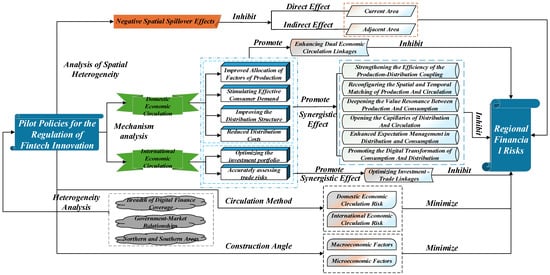
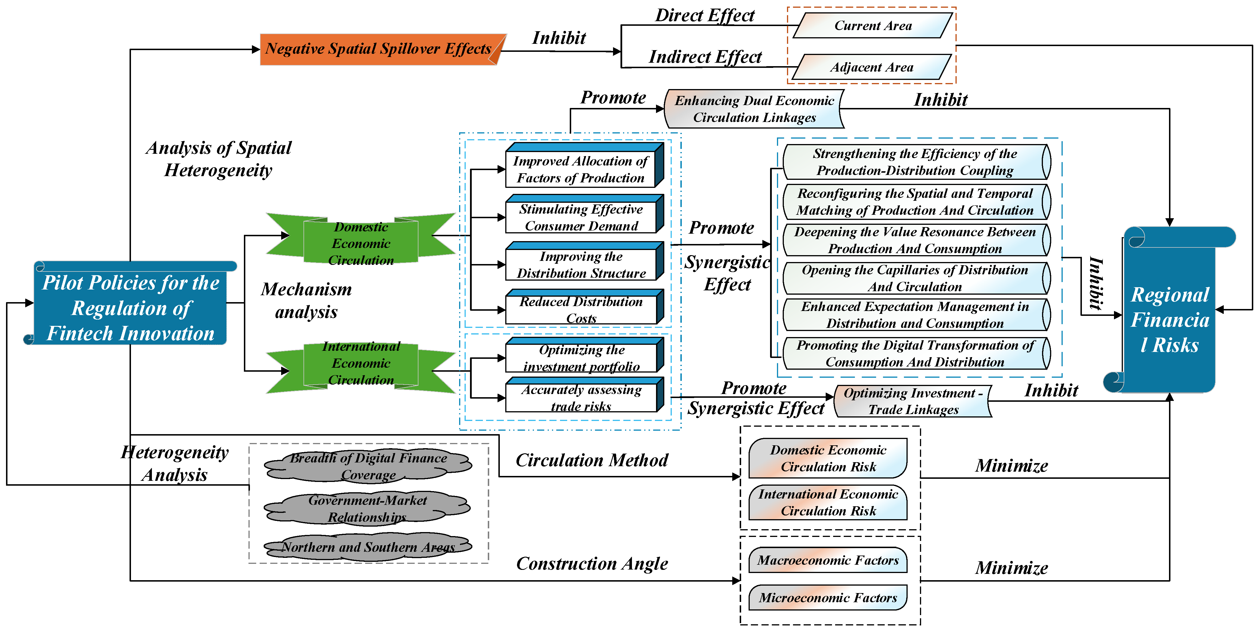
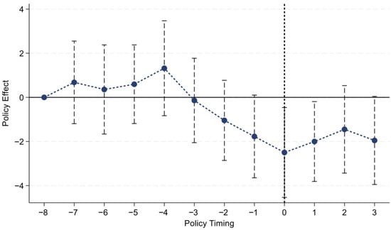
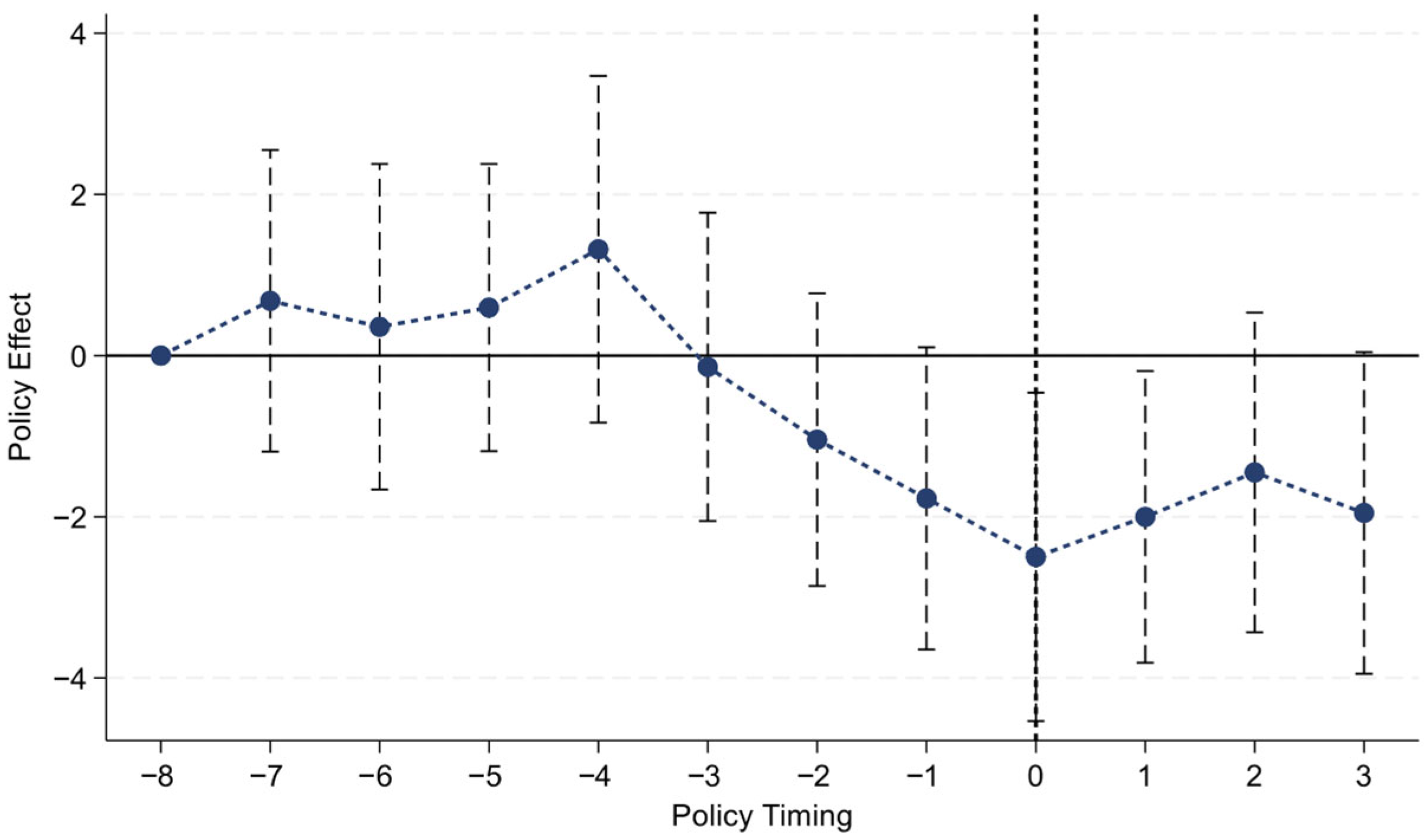
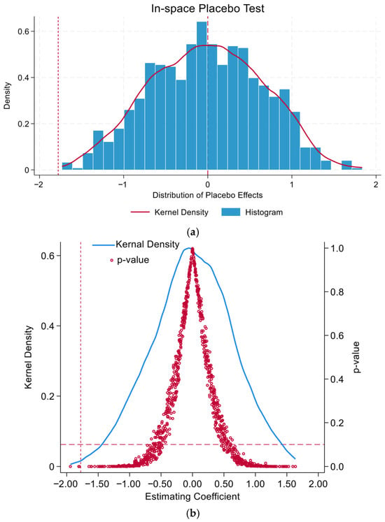
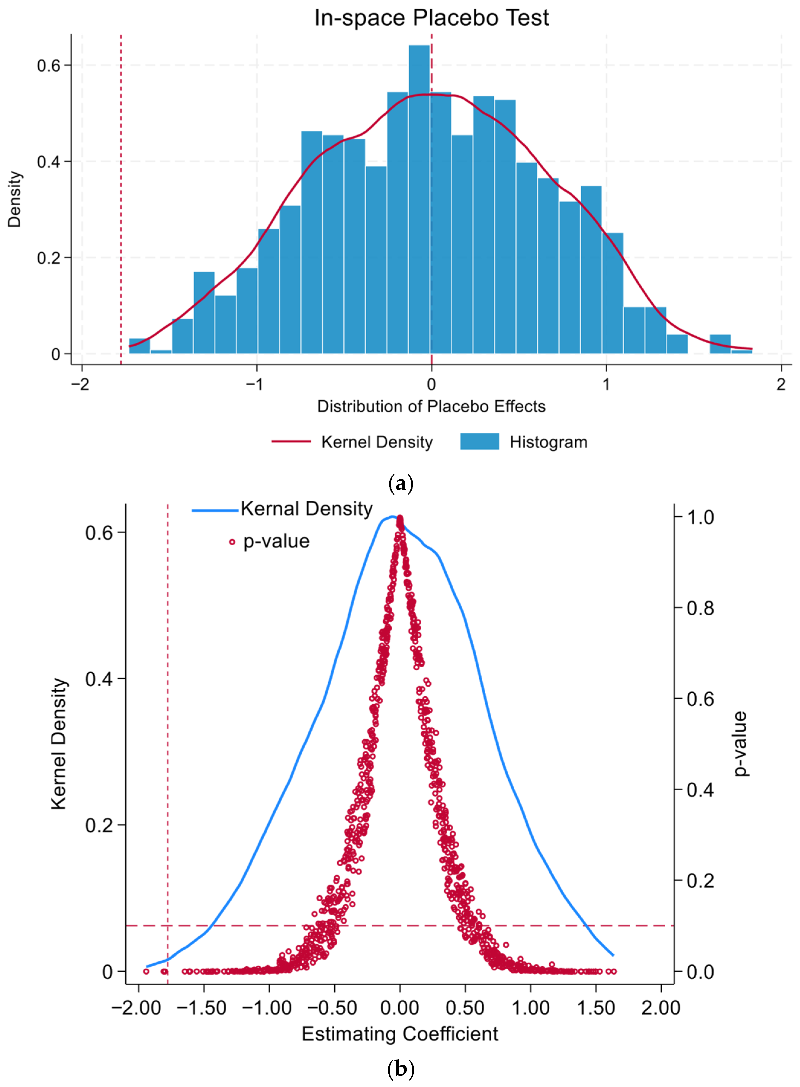
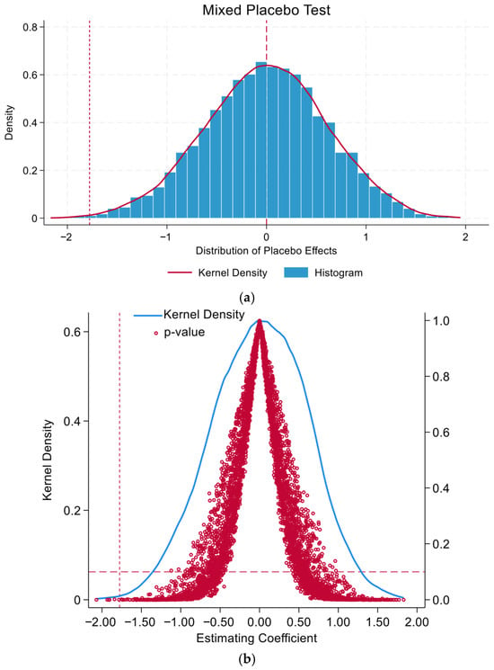
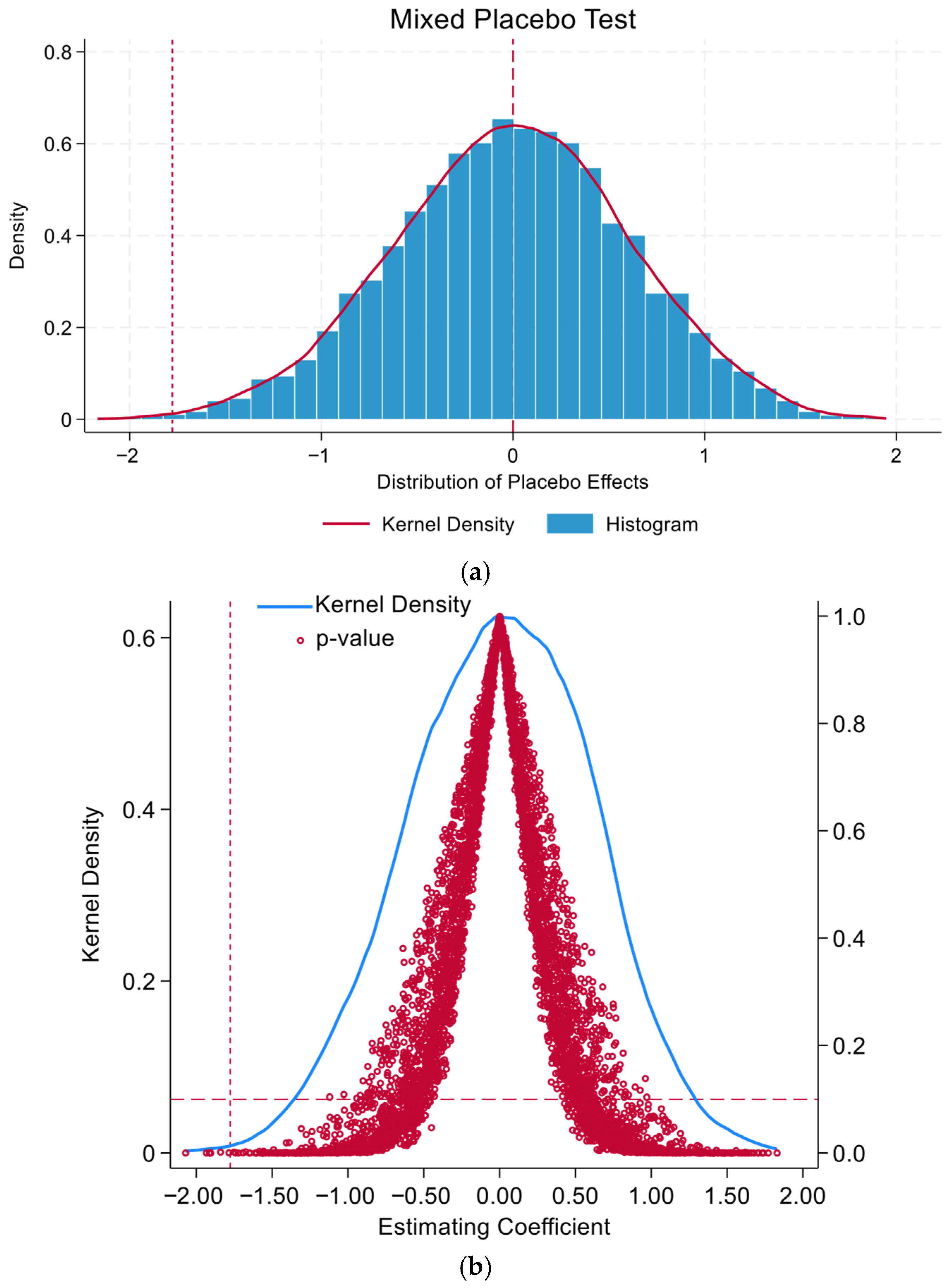
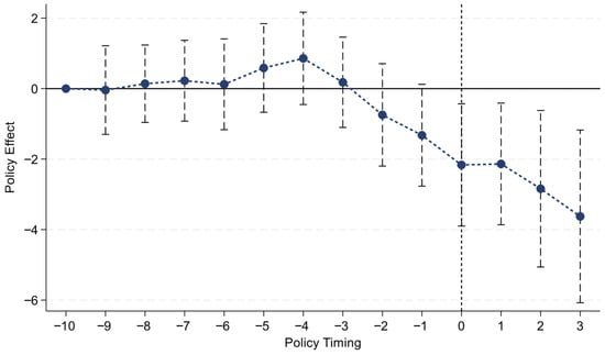
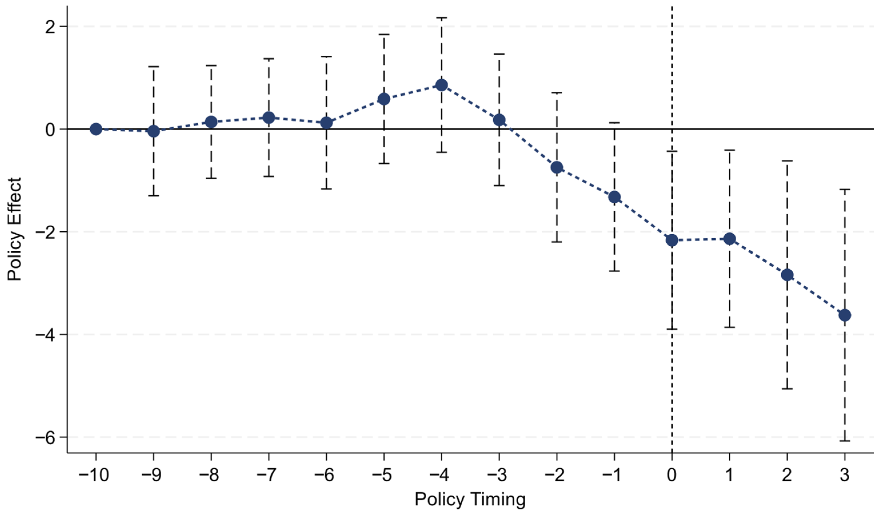
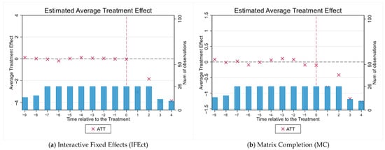
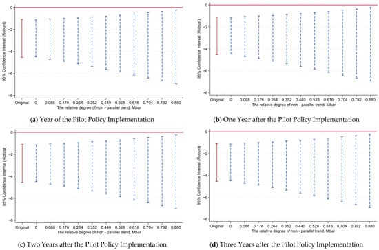
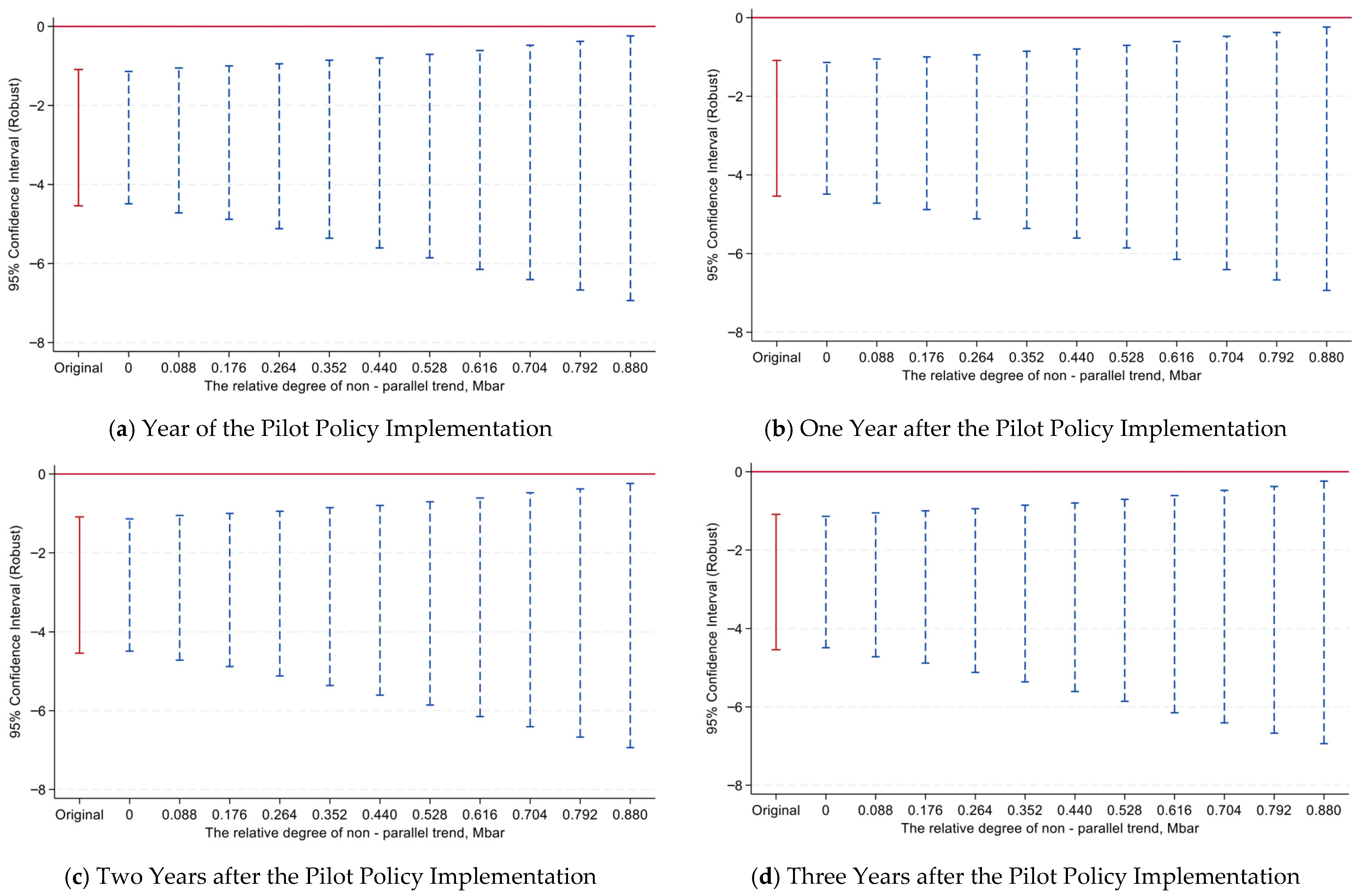
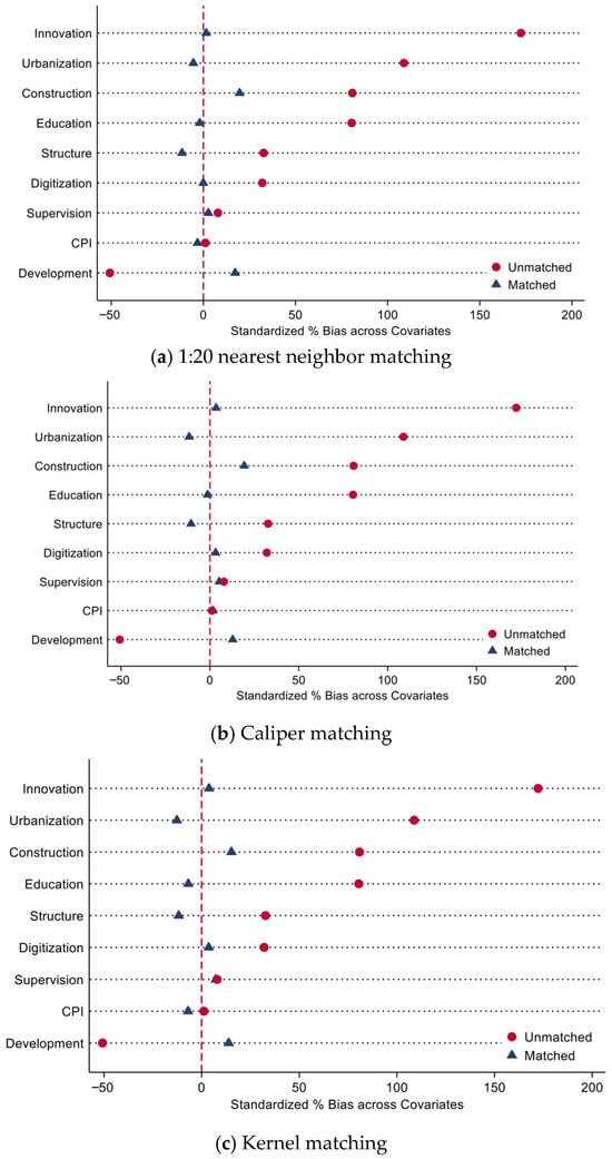
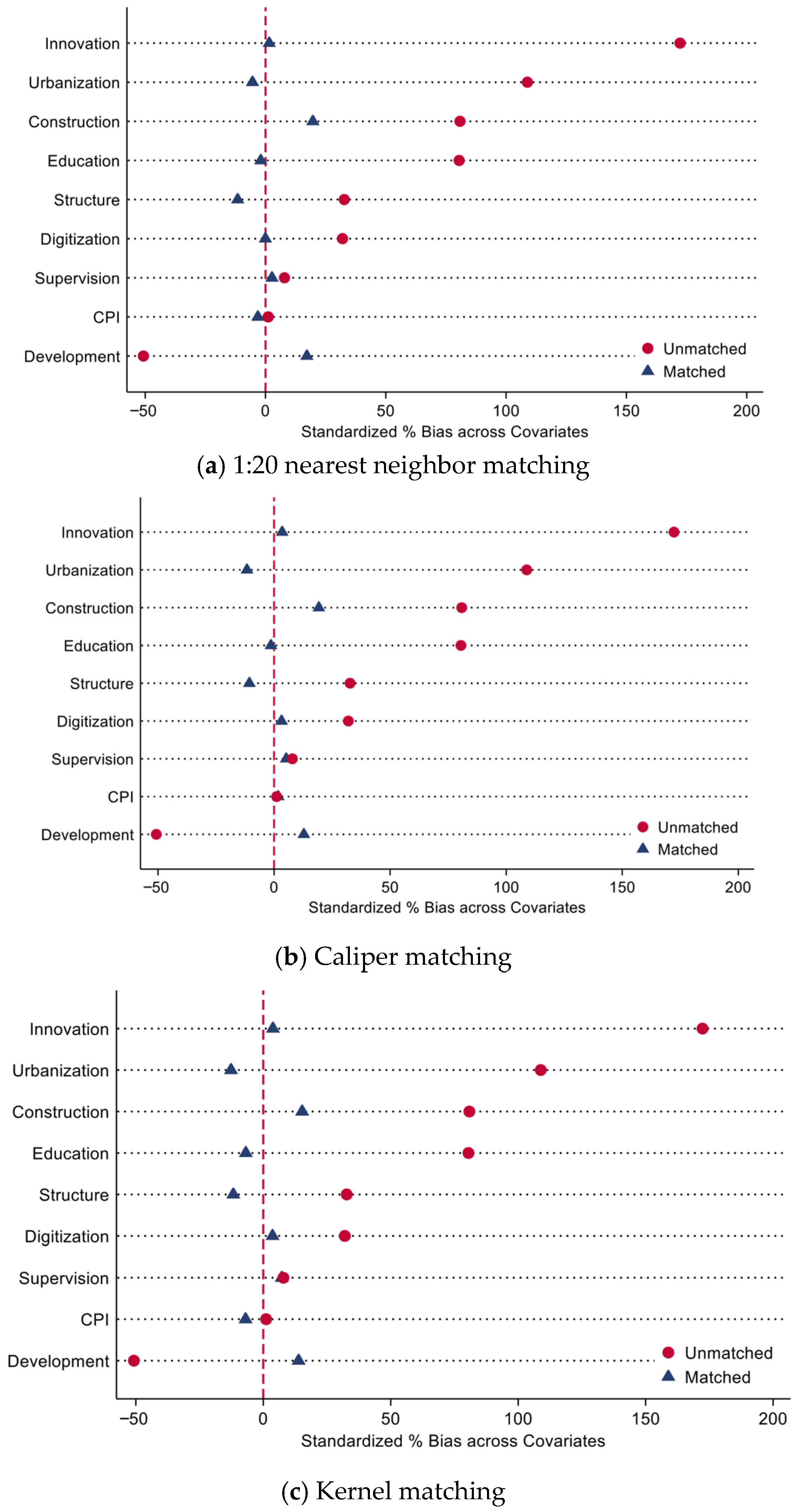
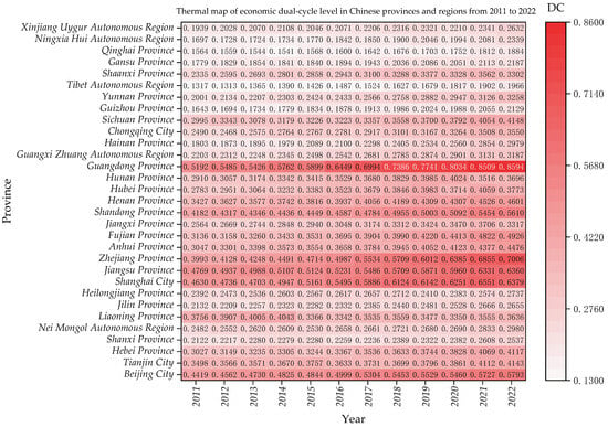
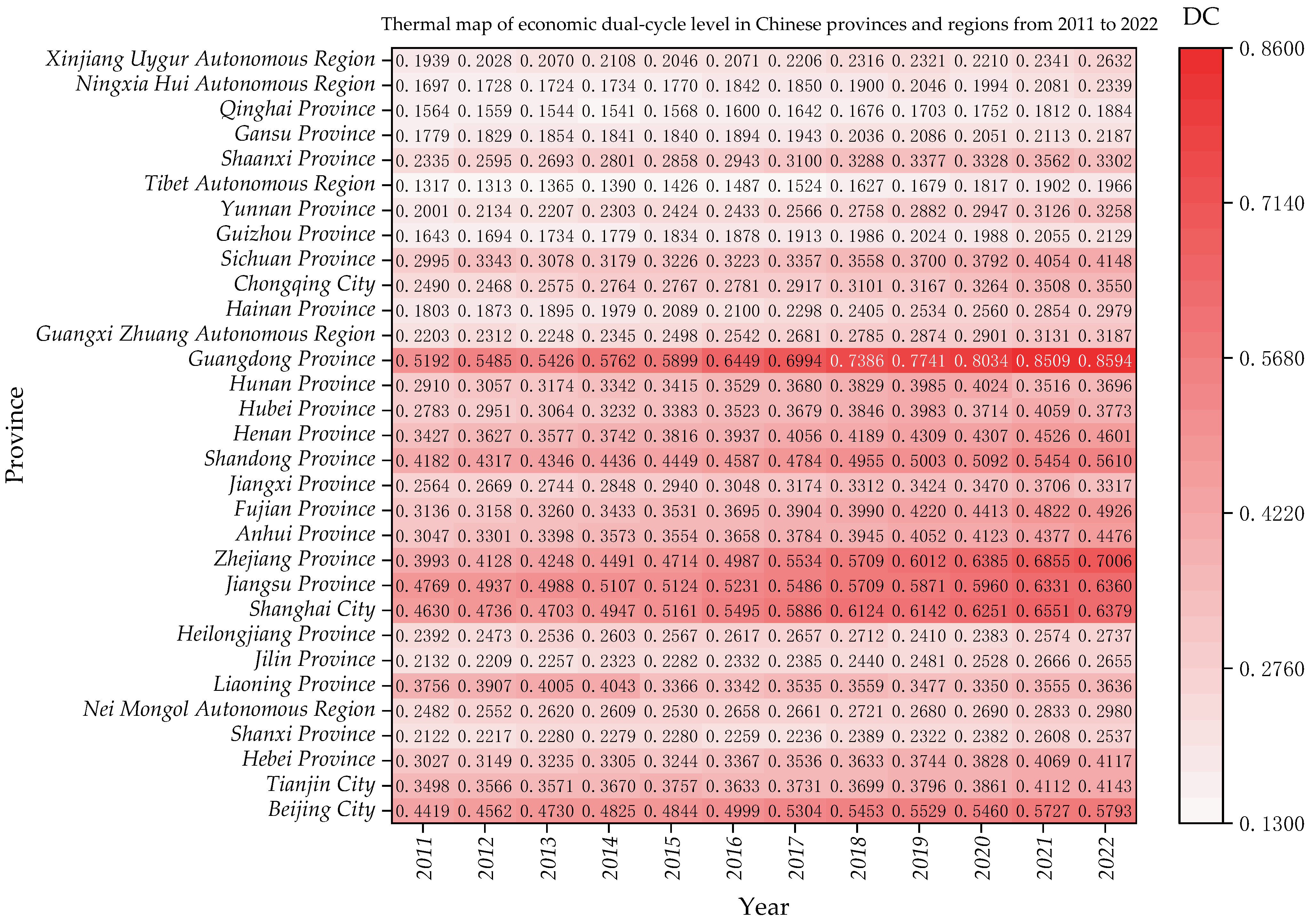
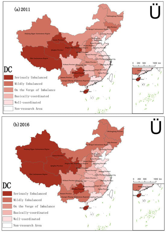
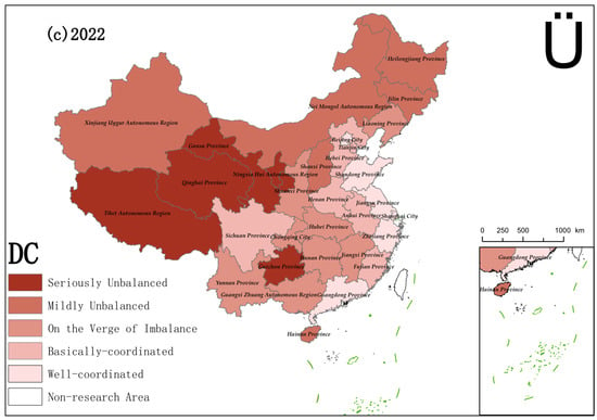
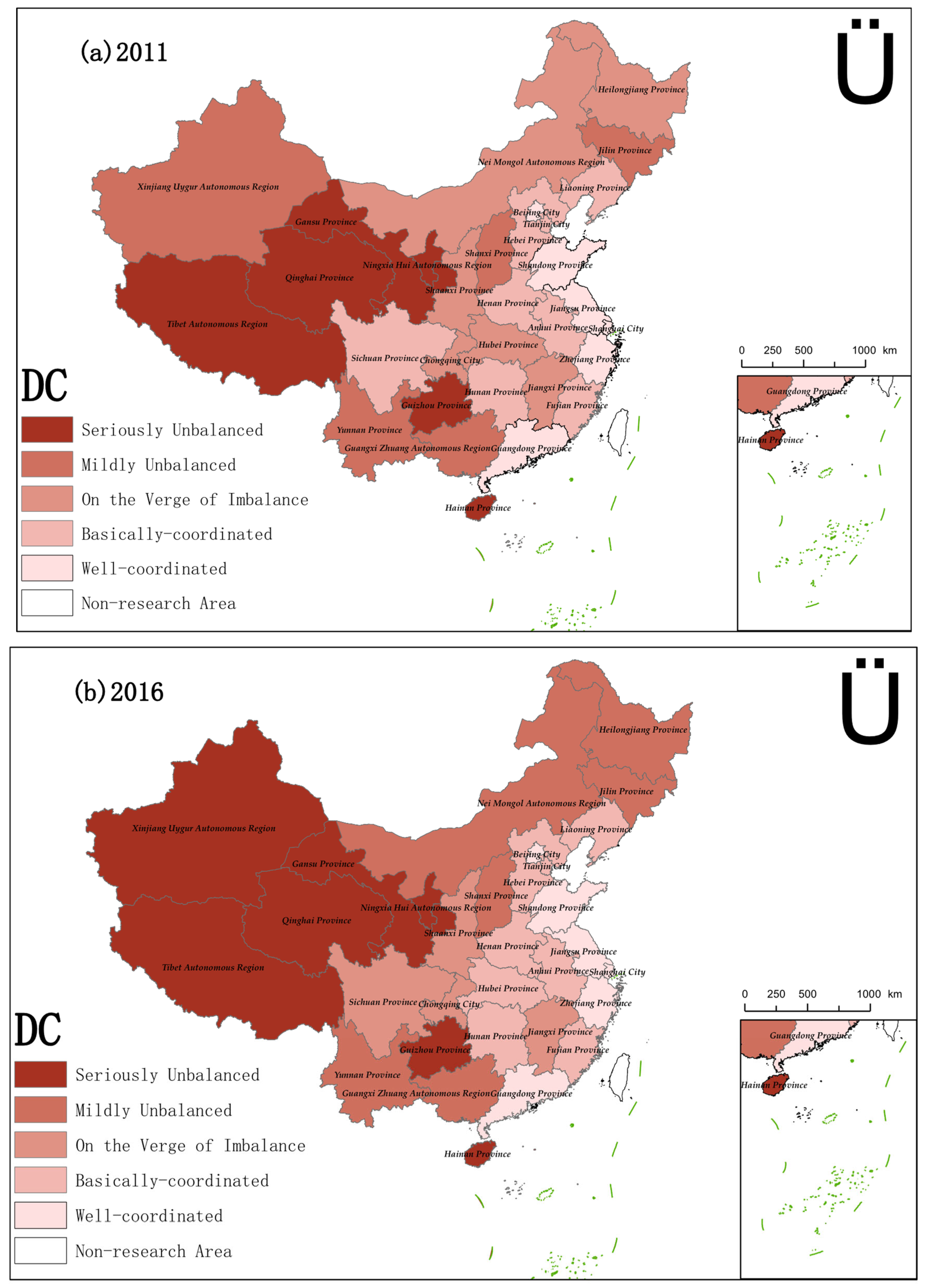
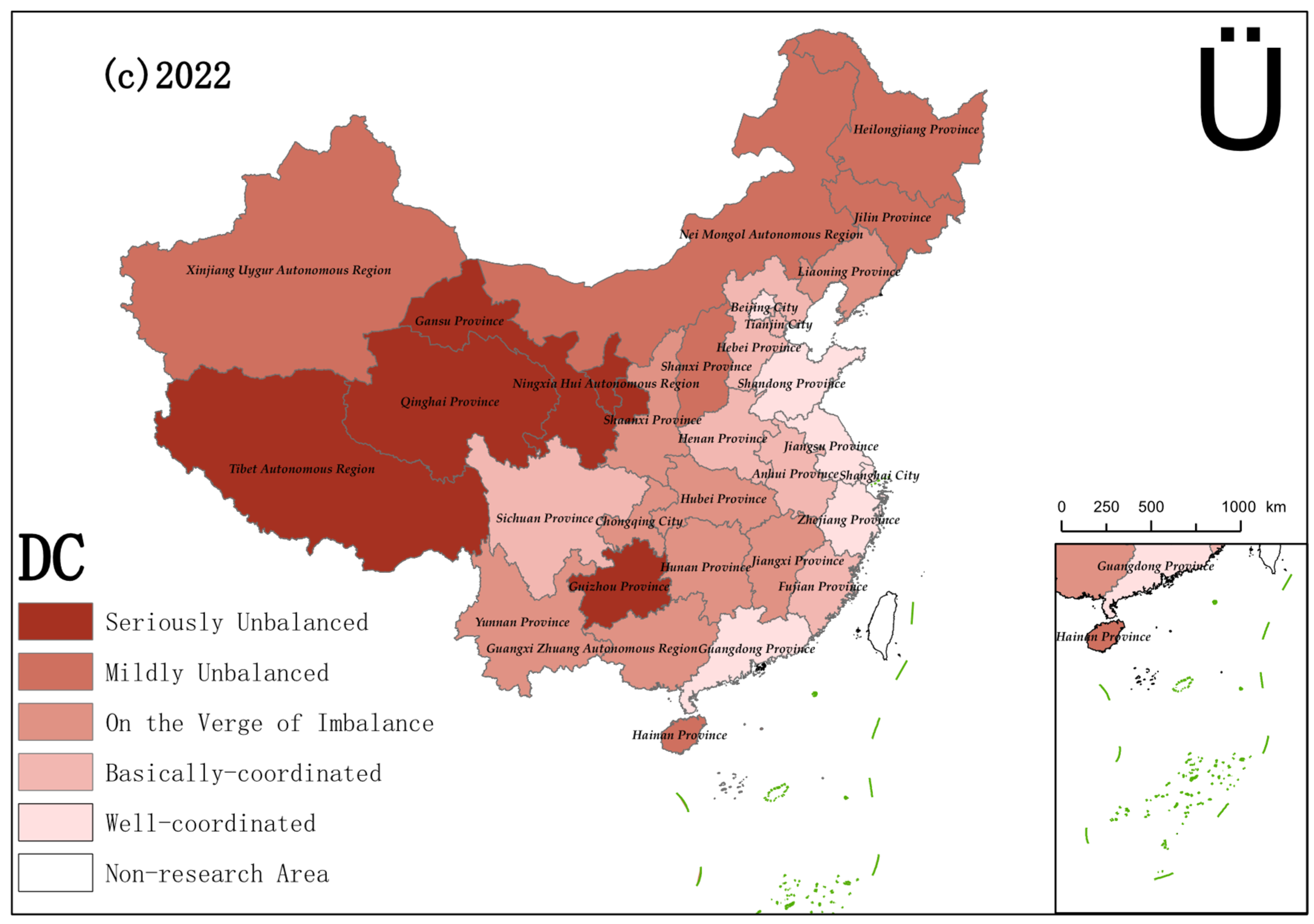
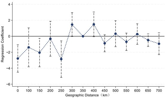
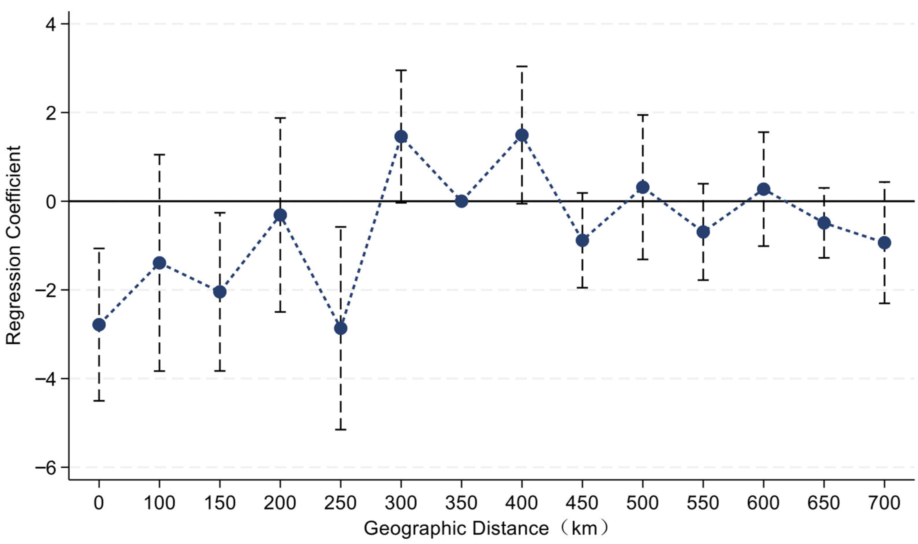

Disclaimer/Publisher’s Note: The statements, opinions and data contained in all publications are solely those of the individual author(s) and contributor(s) and not of MDPI and/or the editor(s). MDPI and/or the editor(s) disclaim responsibility for any injury to people or property resulting from any ideas, methods, instructions or products referred to in the content. |
© 2026 by the authors. Licensee MDPI, Basel, Switzerland. This article is an open access article distributed under the terms and conditions of the Creative Commons Attribution (CC BY) license.