


Highlights
Please indicate how your work links to systems science via your contributions to systems practice, theory, and/or methodology.
- Treats the supply chain information system as a closed decision loop in which every plan is validated against the partners’ shared constraints, recorded, and repaired or rejected before execution, so constraint safety is a property of the loop rather than of the decision engine.
- Contributes a reproducible systems-evaluation method grounded in real multi-plant distribution data: 30-seed paired tests against published routing methods and single-component ablations, stress tests of every simulation assumption, and released code.
What are the main findings and/or the implications of the main findings?
- Pricing delivered demand in the routing objective lowers cost per unit by 33–45%; the learned engine is the fastest high-quality decision maker in the loop, and seeding search with its plan gives the lowest cost of every method tested, including ALNS and OR-Tools.
- Evidence-based validation kept every invalid plan from execution with up to four of five validators faulty, and validate-and-repair kept cost within 0.4% of fault-free operation at a 10% fault rate.
Abstract
Supply chain information systems increasingly need to support decisions, yet Internet of Things (IoT) and blockchain approaches remain largely data-centric. We propose a decision-centric system in which IoT data acquisition, an artificial intelligence decision engine and a blockchain layer form one closed loop: each daily routing plan is optimized jointly for cost, lateness and delivered demand, validated against shared partner constraints and recorded before execution. We evaluated it by simulation on the supply chain logistics problem dataset (41 real customers) over 30 paired seeds. A learned deep Q-network engine with decision-time rollout reduced cost per 1000 units delivered by 24.3% relative to a demand-aware heuristic and 28.0% relative to OR-Tools, deciding in 43 ms; seeding adaptive large neighborhood search (ALNS) with its plan gave the lowest cost, 28.0% below the heuristic and below ALNS alone in 29 of 30 seeds. Joint routing–demand optimization lowered cost per unit by 33–45% relative to a cost-only objective. Under hard time windows, a heterogeneous fleet and eleven other scenarios, rollout stayed 12–32% cheaper than the heuristic in all 130 paired runs, and seeded ALNS was cheapest in every setting. Evidence-based validation blocked every invalid plan with up to four of five validators faulty.
1. Introduction
Existing artificial intelligence (AI)-based approaches to logistics have largely split supply chain management into smaller, disconnected sub-problems. Modern supply chains do not follow the predictable, linear routes of classical models; they are complex, dynamic networks with continuous data generation, fluctuating demand, and operational uncertainty. Supply chain management is consequently moving toward integrated system modeling, optimization, and decision intelligence, in which routing and demand decisions are made jointly, in real time, and validated against a shared set of constraints through a blockchain-based governance mechanism.
Conventional supply chain information systems (SCIS) were designed mainly for data collection, monitoring, and reporting rather than for autonomous decision-making, and they become less useful under disruptive or fast-changing conditions. Supply chains therefore need systems that go beyond collecting and transforming data and act on it directly to streamline logistics operations. Figure 1 shows the unified decision engine proposed in this work, which integrates the Internet of Things (IoT), AI, and blockchain.
Figure 1.
Decision-centric loop: IoT data feed the AI decision engine, whose plans are validated on the blockchain before execution.
IoT gives supply chains continuous, real-time visibility into asset location, condition, and status across the network, a key enabler of informed decision-making [1]. Most IoT-enabled supply chains, however, remain observational rather than prescriptive: they monitor conditions but do not act on them. Blockchain is highly effective at establishing trust and security among heterogeneous partners and at keeping an immutable record of transactions, but it rarely triggers or enforces operational decisions directly and works as a record of data rather than as a check on decisions. Artificial intelligence has separately advanced route planning and demand forecasting, yet these capabilities are usually treated as independent problems rather than as parts of one coherent decision process [2].
We therefore present a decision-centric system that integrates IoT, AI, and blockchain into a single, adaptive, and trustworthy engine for logistics decision-making. Section 1.2 states the research gap and the contributions.
1.1. Background and Motivation
Supply chains involve many interdependent stakeholders, including manufacturers, distributors, logistics providers, and retailers, that must coordinate despite fluctuating demand, unpredictable schedules, and limited resources [3]. Digital technologies, and intelligent systems in particular, increasingly serve as the backbone for coordinating these operations.
IoT provides real-time visibility into asset location, condition, and operational status, but visibility alone has limited value unless a downstream engine turns it into better decisions. Blockchain strengthens trust, security, and transparency among supply chain partners [4]. Although it establishes accountability, blockchain implementations to date rarely execute or validate decisions automatically.
Artificial intelligence, including machine learning and optimization algorithms, offers effective tools for routing and forecasting, but these tools are usually applied in isolation from one another. A routing plan that looks optimal under current conditions can quickly become suboptimal after an unanticipated demand spike.
Our objective is therefore to design a decision-centric system that links IoT data, AI-driven decision-making, and blockchain-based governance, so that logistics operations become adaptive, reliable, and trustworthy. The following subsection defines the research gap and summarizes the paper’s contributions.
1.2. Contributions and Paper Organization
Three gaps remain in the literature reviewed in Section 2. First, integrated IoT–AI–blockchain frameworks use the ledger to secure or trace data, so a decision that violates the partners’ operating constraints is recorded faithfully but not prevented. Second, the AI components of these frameworks optimize forecasting, queueing or routing in isolation rather than the joint decision of which customers to serve and how to route them when capacity is scarce. Third, learned logistics policies are rarely compared on real data with published search methods, so it is unclear when a learned decision engine should be preferred to optimization. From a systems perspective, the missing element is a feedback loop in which sensing, decision, validation and execution are designed and evaluated as one system, with explicit guarantees about what the loop will not execute.
The paper contributes to systems practice and methodology in four ways. First, it proposes a decision-centric supply chain information system in which validation is a gate inside the decision loop: every plan is checked against the partners’ shared constraints, recorded, and repaired or rejected before execution, so that constraint safety is a property of the loop rather than of the decision engine. An evidence-based validation rule, introduced here, requires one honest validator instead of an honest majority. Second, it formulates the daily decision as a prize-collecting capacitated vehicle routing problem whose objective equals the undiscounted return of the sequential process solved by the learned routers, so learned and search-based engines are interchangeable behind one interface, and it shows that integrating demand into the objective lowers cost per unit by 33–45%, the largest effect of any architectural component (the learned engine without demand information lowered it by 12% relative to reactive dispatch, and validation leaves valid plans unchanged). Third, it shows that the learned engine, on its own at short budgets and strengthened by decision-time rollout at longer ones, achieves lower cost than ALNS at every search budget from 0.05 s to 0.1 s on 41 customers, 0.02 s to 1 s on 80 customers and 0.05 s to 2 s on 160 customers (mean decision time); with rollout it is 24.3% cheaper per unit than a demand-aware heuristic and 28.0% cheaper than OR-Tools in 43 ms, while seeding adaptive large neighborhood search (ALNS) with the learned plan gives the lowest cost when more time is available (28.0% below the heuristic and below ALNS alone in 29 of 30 seeds). Fourth, it provides a reproducible evaluation method grounded in real multi-plant distribution data: 30-seed paired tests against published routing methods and single-component ablations, stress tests of every simulation assumption, routing constraint, coverage policy and validator-network size from 4 to 100 validators, and released code that regenerates every number.
The remainder of the paper is organized as follows. Section 2 reviews related work. Section 3 presents the system model and problem formulation (Section 3.1), the architecture (Section 3.2) and the experimental setup (Section 3.3). Section 4 reports the results, Section 5 discusses their implications for systems design, management and sustainability together with the limitations, and Section 6 concludes the paper.
2. Related Work
As supply chains digitalize, IoT, blockchain, and AI have each received considerable research attention, both independently and in combination. Much of this work targets tracking, traceability, and forecasting; comparatively few studies integrate these technologies into a unified, trustworthy decision-making system, and this paper addresses that gap.
2.1. IoT-Enabled Supply Chain Systems
IoT gives supply chains a continuous, real-time feed of operational data, including asset location, condition, and status [5]. Prior studies attribute shorter delivery and lead times, better inventory control, and support for vehicle and warehouse maintenance to this increased transparency. IoT alone is often insufficient, however: knowing that a shipment is delayed does not indicate the appropriate corrective action. Most existing systems lack effective mechanisms for turning high-velocity streaming data into timely decisions; the data volume can overwhelm conventional processing pipelines, and device security and interoperability add further challenges. Real-time visibility is therefore necessary but not sufficient, and without decision support its value is only partly realized. A systematic review of the IoT-supply chain literature is consistent with this shortfall: it finds that most published work remains conceptual or descriptive and that empirical, quantitative evidence linking IoT adoption to measurable supply chain performance is still comparatively scarce [5]. Domain-specific studies report similarly strong but narrowly scoped gains from IoT-based sensing. An intelligent-warehousing system combining IoT with machine learning reports 99% accuracy but limited adaptability to new operating conditions [6], and an embedded-systems framework combines adaptive routing, IoT-enabled demand forecasting, and blockchain supply chain security [7], but applies the ledger to securing supply chain data rather than to validating routing decisions before they are executed.
2.2. Blockchain-Based Supply Chain Systems
Blockchain technology addresses trust concerns among supply chain partners with differing incentives. Its immutable, distributed record lets every participant verify shared information independently [8]. Reported applications include product tracking, counterfeit prevention, regulatory compliance, and process automation through smart contracts, with permissioned participants sharing a consistent, cryptographically secured view of the ledger [4]. In most implementations, however, blockchain serves as a secure record-keeping mechanism rather than a decision-making component, and it rarely extends to making or enforcing operational decisions under the real-time conditions typical of logistics. Scalability to large, high-throughput networks is also a significant challenge: empirical benchmarks of a permissioned blockchain platform show that transaction latency rises with both workload and the number of participating nodes, even as throughput stays stable for a fixed node count, confirming that consensus overhead is a measurable cost rather than a purely theoretical one [9]. Blockchain alone is therefore insufficient to transform logistics decision-making. The same pattern recurs across domain-specific blockchain-IoT deployments that report security, trust, or efficiency gains in pharmaceuticals [10], healthcare [11], general logistics [12,13], construction and building-information-modeling contexts [14], and warehouse-location decisions [15], as well as in supply chain management platforms more broadly [16]; in each case, blockchain remains confined to record verification rather than becoming part of an active decision-making process. A related strand emphasizes privacy rather than decision support, proposing cryptographic approaches that strengthen data confidentiality at the cost of added latency [17].
2.3. AI for Routing and Demand-Aware Logistics
Artificial intelligence has substantially advanced logistics planning and forecasting. Machine learning, deep learning, evolutionary algorithms, and reinforcement learning have been applied to complex problems such as vehicle routing and demand forecasting [3]. In routing, AI-based search methods identify near-optimal paths; in forecasting, learned models estimate future demand from historical and contextual data. Reinforcement learning in particular has been proposed as an alternative to classical search-based routing. A recent deep reinforcement learning formulation of the dynamic and uncertain vehicle routing problem models routing as a partially observed Markov decision process and uses an attention-based network to adapt to real-time demand fluctuations, reporting gains over static routing heuristics under dynamic conditions [18]. For forecasting, federated learning has let supply chain partners predict delivery risk collaboratively without pooling raw order data; it improves prediction for organizations with smaller historical datasets, although the benefit is uneven, since firms with rich order histories still predict better on their own [19]. These techniques have become increasingly accurate and better able to handle complex, non-stationary patterns, improving inventory levels and delivery performance.
Routing and demand forecasting are nevertheless typically solved as separate problems, despite their interdependence: current demand influences routing decisions, and routing decisions in turn affect future demand patterns. Treating them independently, as most existing research does, limits overall system performance. Learned routing heuristics based on attention models approach the solution quality of specialized algorithms on benchmark vehicle routing instances [20], but they solve static instances, without live IoT data or governance of the resulting decisions.
Applied studies show how AI is moving from forecasting into operational supply chain decisions. An AI framework for recycling dormant and obsolete inventory, for example, turns inventory data into disposition decisions for stock that would otherwise be written off [21]. Learned routing policies are one such operational decision, but classical search remains a strong reference for them: adaptive large neighborhood search [22] and guided local search as implemented in OR-Tools [23] are standard tools for rich vehicle routing problems [24], and when capacity is insufficient to serve all customers the problem becomes a prize-collecting, orienteering-type problem in which the planner must also choose whom to serve [25]. A learned router therefore has to be compared with such search methods, not only with constructive heuristics, which this paper does in Section 4.1.
2.4. Integrated and Emerging Approaches
Fewer studies attempt to integrate all three technologies at once. One recent framework combines IoT edge controllers, blockchain-based transaction logging, and an AI-based optimizer to manage service-request queues in smart-city logistics, reporting improvements in queue length, resource utilization, and end-to-end delay [26]. Unlike the present work, it optimizes queue scheduling rather than joint vehicle routing and demand-aware decision-making, and its blockchain layer is not evaluated as a source of decision-validation latency. A related but distinct line of work models the supply chain itself as a real-time, IoT-fed digital twin, a simulation-and-optimization layer used to anticipate and mitigate disruption risk and improve structural resilience [27]. This approach shares our emphasis on continuously feeding IoT data into a live decision model, but it does not incorporate blockchain-based validation or reinforcement-learning-based routing. Across this body of work, IoT, AI, and blockchain are more often combined pairwise, or integrated around a different decision objective such as queueing or disruption resilience, than around the joint routing-and-demand decision problem with blockchain-validated execution addressed here. Several reviews and conceptual studies survey this convergence without implementing or evaluating an integrated system of their own. A web-content-mining-based review of IoT decision-support systems in supply chains and logistics offers useful decision insights but no real-time execution [28]; broader reviews of blockchain-IoT supply chain applications report positive impact and improved flexibility without implementation or experimentation [29,30]; and a review focused on blockchain-IoT-AI convergence reports improved traceability but does not arrive at a unified model [31]. A conceptual account of supply chain digitization likewise reports improved resilience but stops short of incorporating AI [32]. Among empirical studies that combine more than one of the three technologies, a machine-learning-and-blockchain system improves prediction accuracy without adding a decision layer [33], and a vaccine supply chain system integrating machine learning, IoT, and blockchain improves forecasting at the cost of increased system complexity [34]. Together, these reviews and multi-technology studies reinforce that the specific combination pursued here, joint routing-and-demand decision-making validated through blockchain, remains largely unaddressed.
Motivated by this gap, we propose a decision-centric system that jointly integrates IoT, AI, and blockchain to support coordinated supply chain decision-making. Table 1 summarizes the relevant literature and the specific gaps this paper addresses; the problem is formalized in Section 3.1.
Table 1.
Summary of the existing literature, with methods, results, and research gaps.
Table 2 compares the integrated frameworks closest to this work on the properties that define a decision-centric system. The frameworks differ from the present one in the role given to the blockchain and in the decision that is optimized. In refs. [7,33,34] the ledger secures or traces data while the AI component forecasts or predicts; in ref. [26] the AI component schedules service queues; and the digital twin of [27] and the learned routers of [18,20] optimize decisions without a validation layer. The theoretical contribution of the present architecture lies in this combination: the decision itself is the object that is optimized jointly over routing and demand, validated against constraints agreed among the partners, recorded, and repaired or replaced before execution, so that constraint safety becomes a property of the closed loop rather than of any single decision engine.
Table 2.
Comparison with integrated frameworks on the properties of a decision-centric system.
3. Materials and Methods
This section formalizes the system and the decision problem (Section 3.1), describes the architecture (Section 3.2), and details the experimental setup (Section 3.3).
3.1. System Model and Problem Formulation
This section presents a formal mathematical framework for the proposed decision-centric supply chain information system. The methodology combines system modeling, optimization theory, and decision intelligence for dynamic, uncertain environments, and centers on a unified decision function that jointly optimizes routing and demand-aware logistics under blockchain-based validation constraints. Figure 2 gives a graphical overview of the end-to-end workflow of the study.
Figure 2.
Workflow of the study: data, state, decision, validation, execution and feedback.
Table 3 lists the notation used in the paper.
Table 3.
Notation.
We model the AI-driven supply chain optimization framework as a directed graph that captures the relationships among warehouses, distribution centers, and customers through interconnected transportation links. The model includes dynamic state representation, IoT-based data streams, and stochastic transition dynamics to reflect real-world uncertainties. Bringing demand, cost, location, and resource availability into a unified state space allows the framework to support intelligent and adaptive decision-making for efficient logistics operations.
3.1.1. System Model
Let the supply chain be represented as a directed graph:
where
G = (V,E)
- V = {v1,v2,…,vn} represents nodes (warehouses, distribution centers, customers)
- E = {eij} represents edges (transportation links)
- State Representation
The system state at time t is defined as:
where
St = {Lt,Dt,Ct,Rt}
- Lt = {li(t)}: location states
- Dt = {di(t)}: demand vector
- Ct = {cij(t)}: transportation cost matrix
- Rt = {rk(t)}: resource availability
- IoT Data Stream Model
St+1 = T(St,At,ωt)
- At: decision/action
- ωt: stochastic disturbance
3.1.2. Problem Formulation
Define the decision variable:
where
Total trip capacity is smaller than total demand (Section 3.3.1), so not every customer can be served on a given day and the planner must also choose which customers to serve. The routing problem is therefore a prize-collecting capacitated vehicle routing problem with a route-duration limit and soft due times, of the team-orienteering family [24,25]. In addition to the arc variables akij, we use the service indicator yik ∈ {0, 1}, the planned load qik ≥ 0 and the arrival time τik of customer i on trip k.
- Objective Function
Multi-objective optimization:
(1) Routing Cost
(2) Time Delay
(3) Delivered Demand
Z1 is the freight charge of each trip’s consolidated weight under its carrier’s real weight-banded rates plus the local distance cost, Z2 the lateness of the stops made, and Z3 the demand actually delivered, which replaces the forecast-error term of the initial formulation; α4 is an optional coverage weight (Section 4.6). The weights are α1 = 0.1, α2 = 0.5, α3 = 3.0 and α4 = 0, and Jt denotes Z evaluated for day t.
- Constraints
Flow Conservation:
Capacity Constraint:
Single Visit:
Time Propagation and Subtour Elimination:
Route Duration:
Hard Time Windows (variant, Section 4.5):
τik ≤ δi + M(1 − yik) ∀i,k
Binary Constraint:
Constraint (13) allows at most one visit per customer and day; it replaces the requirement of the initial formulation that every customer be visited, which cannot hold when capacity binds. Loads may be partial (12), and (14) also eliminates subtours. Plans are built from observed demand and executed against true demand.
3.1.3. Decision-Centric Framework
The decision pipeline is defined as:
Prediction Function
Decision Function
Policy Optimization
3.1.4. AI-Driven Decision Engine
- Routing Optimization (RL Formulation)
- Demand Forecasting Model
3.1.5. Optimization Model
- Multi-Objective Formulation
minZ = (Z1,Z2,Z3)
A* ∈ {A:∄A′ such that Z(A′)≺Z(A)}
= Z + λ1(Capacity) + λ2(Flow)
minEω[Z(St,At,ω)]
To make explicit which formulations are solved in the experiments: the daily problem (7)–(17) is solved by every decision engine, directly by ALNS and through the equivalent sequential process (22)–(24) by the learned routers, and the validation model (33)–(39) is implemented as stated. The pipeline and policy formulations (18)–(21) and (26) describe the decision problem as a whole, which the learned routers optimize in expectation; the generic forecasting model (25) is instantiated by the exponentially weighted forecast (78); and the multi-objective, Lagrangian, stochastic and constraint-relaxation forms (27)–(32) state the general problem class and are not solved directly. Likewise, in Section 3.3, Equations (66)–(76) and (79)–(81) state the general data, sensing and forecasting models, of which the evaluation uses the observation model (77)–(78), and (102)–(106) characterize the baselines schematically.
3.1.6. Blockchain-Based Validation Model
- Decision Record
Bt = H(At‖St‖t)
- Validation Function
At ∈
Trusti(t) = β Trusti(t − 1) + (1 − β) 1[vi(t) = maj(t)]
Because membership of is decidable from the plan itself, a reject vote can carry a violation witness ωj = (constraint, trip, stop) that any node can re-check. The evidence rule introduced in this revision rejects a plan whenever at least one witness verifies, ignores reject votes whose witness does not verify, and scores validators against the verified outcome (At) instead of the majority:
Safety then requires one honest validator rather than an honest majority. A rejected plan is replaced by the reactive dispatch plan or, in the validate-and-repair mode, minimally repaired (phantom and repeated stops removed, loads clipped, trips truncated to return within the shift), so the corrected execution rule is
- Final Decision Execution
Trust score is defined here as a per-validator exponential moving average of agreement with the consensus outcome, so it is conceptually distinct from the consensus mechanism above: the consensus mechanism determines whether one specific decision is accepted in a single round, whereas trust score tracks a validator’s reliability across many rounds. Figure 3 shows the decision framework as implemented in the evaluation, tracing how real-time data move through the system from raw observations to executed routing decisions.
Figure 3.
Decision framework as implemented: IoT-observed demand, AI routing, blockchain validation of each daily plan, execution or fallback, and training feedback.
In the framework of Figure 3, the IoT data layer supplies each customer’s observed demand, with missing readings filled by an exponentially weighted moving-average forecast. The AI routing engine, a tabular Q-learning router or a candidate-scoring deep Q-network trained on a joint cost, delay, and delivered-demand reward, turns this state into a daily routing plan. Five validators check the plan against the shared constraints (capacity, shift length, one visit per customer, valid customer identifiers, and loads within observed demand) and accept it by majority vote among validators whose trust score is at least the threshold; every decision is recorded in a SHA-256 hash chain. An accepted plan is executed against true demand, a rejected plan is repaired or replaced by the reactive dispatch plan, and the executed outcomes update the router during training (Section 3.3).
3.2. Proposed Decision-Centric SCIS Architecture
The proposed architecture puts a decision-centric paradigm into operation by integrating IoT-based data acquisition, AI-driven decision intelligence, and blockchain-based governance in one system. Unlike traditional data-centric architectures, it treats decision-making as its core function, supporting real-time, adaptive, and trustworthy logistics operations. A layered design provides modularity, scalability, and interoperability across heterogeneous supply chain environments.
3.2.1. Overall Architecture
The overall architecture is structured into four primary layers. Figure 4 illustrates a blockchain-enabled decision-validation framework in which optimized decisions are verified through smart contracts and consensus algorithms. Decision nodes process and validate outcomes based on cost, delay, and trust, and the blockchain ledger provides secure, immutable, and distributed record-keeping.
Mathematical Flow
𝒜 = {LIoT,LData,LDecision,LBlockchain}
Figure 4.
Decision validation: each plan is checked against the shared constraints, recorded, and released or rejected.
Each layer performs a specialized function within the decision-centric workflow, which keeps concerns separated while the system components remain integrated.
3.2.2. IoT Layer: Data Acquisition and Streaming
The IoT layer is the foundation of the architecture and acquires data in real time from distributed supply chain entities. It consists of interconnected devices such as sensors, global positioning system (GPS) trackers, radio-frequency identification (RFID) tags, and embedded systems that continuously monitor logistics operations.
- Data Model
Xt = ϕ(Sensor,Network,Time)
The captured data include vehicle locations, shipment conditions, environmental parameters, and inventory states, and this real-time stream supports continuous monitoring and situational awareness.
To handle high-velocity data, streaming frameworks are employed:
where ψ represents filtering, aggregation, and preprocessing operations.
- Challenges Modeled
The IoT layer thereby keeps an up-to-date representation of the supply chain state for downstream decision-making.
3.2.3. Decision Intelligence Layer: AI Engine Integration
The decision intelligence layer is the core of the proposed architecture: it turns processed data into optimized decisions using machine learning models, reinforcement learning policies, and optimization techniques.
- State Input
St = f(Xt)
This layer jointly optimizes routing and demand-aware logistics to capture their interdependencies, with reinforcement learning models adapting routing strategies dynamically:
Feedback Loop
Q(s,a) → π(a∣s)
θt+1 = θt − η ∇θ(θt)
Combining predictive and prescriptive analytics lets the system respond to real-time changes such as demand fluctuations and traffic conditions.
The decision layer hosts interchangeable engines behind the same interface: the learned routers, which decide in milliseconds and can spend additional time on decision-time rollout, and an adaptive large neighborhood search (ALNS) engine that optimizes (7) directly and can start from the learned engine’s plan (Section 3.3.3). Because all engines optimize the same objective and their plans pass through the same validation, the engine can be chosen by decision cadence without changing the rest of the system.
3.2.4. Blockchain Governance Layer: Smart Contracts and Validation
The blockchain layer ensures trust, transparency, and accountability in decision-making, and unlike traditional implementations, it governs decisions rather than only data.
- Decision Encoding
Bt = H(At‖St‖t)
Trusti(t) = β Trusti(t − 1) + (1 − β) 1[vi(t) = maj(t)]
Smart contracts enforce constraints such as capacity limits, delivery deadlines, and stakeholder agreements:
At ∈
Blockchain thereby becomes an active decision-governance mechanism rather than a passive ledger.
In a deployment the validators would be operated by the supply chain partners and reach agreement through a Byzantine fault-tolerant protocol; Section 4.9 quantifies its latency and message cost for 4 to 100 validators. The shared constraints are the operational terms the partners agree on, so the ledger acts as an executable agreement on what a valid decision is.
3.2.5. Decision Workflow: End-to-End System Operation
Figure 5 shows how the complete workflow integrates all layers into a continuous decision-making pipeline.
Figure 5.
End-to-end decision workflow: data acquisition, state construction, prediction, optimization, validation, and execution, with closed-loop feedback.
- Stepwise Flow
- Step 1: Data Acquisition
Xt ← IoT
St = f(Xt)
St+1 = T(St,At,ωt)
This closed loop ensures continuous adaptation and learning, allowing the supply chain to respond dynamically to changing conditions.
3.3. Experimental Setup
This section describes the experimental design we used to evaluate the proposed decision-centric supply chain information system. The setup combines real-world datasets, simulated IoT data streams, AI-based decision models, and blockchain-based validation mechanisms, with the aim of rigorously assessing system performance under realistic, dynamic logistics conditions.
This section describes how the system was evaluated: the real data that ground the simulation (Section 3.3.1), the simulated IoT streams (Section 3.3.2), the decision engines and their training (Section 3.3.3), the ledger implementation (Section 3.3.4), and the metrics and baselines (Section 3.3.5). Table 4 separates the components taken from real data from those that are simulated or assumed, and states where the sensitivity of the results to each assumption is tested.
Table 4.
Real, assumed and simulated components of the evaluation.
3.3.1. Dataset Description
The experimental evaluation uses the supply chain logistics problem dataset (Kalganova & Dzalbs, Brunel University London, 2019) [36], a real historical multi-plant distribution network with real plant-to-port connections, real per-plant daily capacities, a real weight-banded freight-rate schedule per carrier, and 9215 real historical orders. How we map this dataset onto the system’s routing/demand/cost interface is detailed below; the dataset was introduced with the ant colony optimization study of [37].
The real dataset used in Section 4 comprises seven relational tables: OrderList (9215 real historical orders, each with a plant code, customer ID, order date, product ID, unit quantity, and shipment weight), FreightRates (a weight-banded rate schedule per carrier and port-pair, giving a minimum charge and a per-unit-weight rate for each weight bracket), PlantPorts (which plants connect to which ports), WhCapacities (each plant’s real daily throughput capacity), WhCosts, ProductsPerPlant, and VmiCustomers. This evaluation uses the network’s dominant plant, PLANT03, as the depot: it accounts for 8541 of the dataset’s 9215 orders (92.7%) and serves 41 of the dataset’s 46 distinct real customers, so almost the entire real order volume and customer base is represented.
Each of the 41 real customers’ empirical demand distributions is built directly from that customer’s own historical order quantities, bootstrap-resampled once per simulated day and winsorized at the 95th percentile of PLANT03’s order quantities (12,331 units) to control a small number of extreme bulk orders without discarding the customers who place them. Each customer’s unit weight is the median ratio of shipment weight to unit quantity over its orders, and its service level (door-to-door, DTD; door-to-port, DTP; or customer-referred freight, CRF) is its most frequent level. Three vehicle trips are dispatched per day, and the per-trip capacity is set to 0.55 of the mean total daily demand divided by the number of trips (22,133 units), so capacity binds and not all demand can be served. Each trip’s carrier is drawn at PLANT03’s real usage shares (V444_0: 68.4%; V444_1: 23.2%; V44_3: 8.3%). Its freight charge is computed from that carrier’s real weight-banded rate table for the PORT04 to PORT09 lane (DTP rates for V444_0 and DTD rates for V444_1, matching how each carrier is used in the order history) as the maximum of the minimum charge and rate times consolidated trip weight, taking the cheapest rate row where several exist and never charging more than the next weight bracket would. Carrier V44_3 carries only CRF, so its trips incur no freight charge to the shipper. Because the source data contain no customer coordinates, customers are placed uniformly at random in a 100 km by 100 km region with the depot at its center, with a new layout for each seed. Vehicles travel at 40 km/h with 0.25 h of service per stop within an 8 h shift; due times are 3 h (DTD), 5 h (DTP), and 8 h (CRF) after dispatch; and local delivery costs 0.02 cost units per km. These assumed parameters are listed in Table 5 and in the released code, and their influence is tested in Section 4.7. Local delivery is a substantial share of daily cost, so routing decisions affect both which demand is served and what it costs.
Table 5.
Key real quantities extracted from the dataset for the simulation.
No classification or regression labels are used from this dataset; it grounds the simulation’s routing graph, demand, capacity, and cost structure rather than serving as a supervised-learning training set. The 800/200 epoch training/held-out test split used in Section 4 applies to the simulated decision epochs the routing policies are trained and evaluated on, not to a split of the historical orders themselves. Table 5 summarizes the real quantities extracted from the dataset for the simulation, and Table 6 summarizes the key fields used from its source tables.
Table 6.
Key fields of the supply chain logistics problem dataset.
- Dataset Representation
Let the dataset be defined as:
where
- li: location coordinates
- di: demand values
- ti: timestamps
- cij: transportation cost between nodes
- Dataset Integration
combined = 1 ∪ 2
train,test = split(,ρ)
ρ = 0.8
The datasets provide information on shipments, orders, transportation costs, and delivery timelines, enabling realistic modeling of supply chain operations.
3.3.2. IoT Data Simulation
Because real-time IoT streams are not directly available, we developed a simulation framework to emulate dynamic data generation.
- IoT Stream Model
li(t + 1) = li(t) + vi(t)Δt + εt
εt∼(0,σ2)
P(xi(t) = ∅) = pm
In the evaluation, each customer’s observed demand is its true demand multiplied by (1 + ε), with ε ~ N(0, 0.052) and truncation at zero, and a reading is missing with probability 0.02, in which case it is replaced by an exponentially weighted moving-average (EWMA) forecast (smoothing factor 0.3) of that customer’s past observed demand. Routing plans are built from observed demand and executed against true demand, so observation error propagates into delivered quantities and cost. The sensitivity analysis (Section 4.7) varies the noise level from 0% to 40%.
Formally, the observed demand and the forecast used to fill missing readings are
3.3.3. AI Model Implementation
The decision intelligence layer consists of two core components: demand prediction and routing optimization. Two learned routers instantiate the routing component. Both build each vehicle trip one stop at a time from the customers that are unvisited, have positive observed demand, and can be reached and returned from within the shift; a trip ends when its capacity is exhausted or no customer remains feasible.
- Demand Prediction Model
Q(s,a) ← Q(s,a) + α[r + γmaxQ(s′,a′) − Q(s,a)]
The neural router minimizes the Huber temporal-difference loss with a target network θ− over the replay buffer 𝓑:
Reward Function
Policy
Integrated Decision Model
The first router is tabular Q-learning. Its state encodes the vehicle’s current position together with a five-bin discretization of the fraction of total observed demand not yet served, and its action is the next customer to visit. The identity of the specific unvisited customers is therefore not part of the state.
The second router is a deep Q-network with a shared candidate-scoring network. For each feasible customer, a ten-dimensional feature vector is formed: distance from the current position, distance back to the depot, slack to the customer’s due time, remaining capacity and shift time, share of customers still unvisited, local density of unvisited customers, the customer’s observed demand, the load it would receive, and the marginal freight-plus-distance cost of serving it. A multilayer perceptron (MLP) with two hidden layers of 32 rectified linear (ReLU) units scores each vector, and the highest-scoring customer is chosen. Because the candidate set itself encodes which customers remain unvisited, and the same network scores every candidate, the router has 1441 parameters regardless of network size. It is trained with experience replay (buffer 20,000, batch 64), a target network synchronized every 500 updates, a Huber loss, the Adam optimizer (learning rate 10−3), and an exploration rate that decays linearly from 1.0 to 0.05 over the first 60% of training.
Both routers receive a per-stop reward r = −α1·Δcost − α2·delay + α3·delivered/Q, where Δcost is the marginal freight-plus-distance cost of the stop, delay is its lateness in hours, delivered is the quantity actually delivered, and Q is the vehicle capacity (α1 = 0.1, α2 = 0.5, α3 = 3.0). This is the per-step form of the objective in Section 3.1.2: rewarding delivered quantity at each stop is equivalent, up to a constant per day, to penalizing unmet demand. The separate configurations use the cost term alone and receive no demand information: the tabular separate state replaces the remaining-demand fraction with the fraction of customers unvisited, and the neural separate router has its demand and load features set to zero and its marginal-cost feature limited to distance. Both routers are trained for 800 simulated days and evaluated, without exploration or learning, on 200 held-out days.
The freight increments in (84) telescope to the trip’s freight charge, and the return leg is charged at the last stop, so the undiscounted return (γ = 1) of a day’s plan equals −Jt, and maximizing it is the same problem as minimizing the expected daily objective (7). The routers are trained with γ = 0.9, which weights the stops of a day unequally and therefore optimizes a discounted surrogate of (7) with lower-variance bootstrapped targets. The discount factor affects training only: every reported result is the undiscounted objective (7) and its metrics evaluated on the executed plans, and the rollout and ALNS engines evaluate (7) exactly. With γ = 0.99, the setting closest to the undiscounted objective, the router still undercut the demand-aware heuristic in every seed (Section 4.4). Because rewards are computed from the executed outcome, the routers learn to minimize the objective under observation noise.
Table 7 summarizes the states, actions, objectives and settings of the decision engines.
Table 7.
Decision engines: state, actions, objective and settings.
Training follows the same loop for both routers. On each of 800 simulated days, a day’s demand and carriers are drawn, the IoT stream is generated, the router builds the plan with ε-greedy exploration, the plan is executed against true demand, the per-stop rewards are computed from the executed outcome, and the router is updated (one tabular update per stop, or one minibatch update of the neural router per stored transition after a 500-transition warm-up). Every 80 days the current policy is evaluated greedily on 20 validation days that are disjoint from the test days, which yields the learning diagnostics of Section 4.4. After training, exploration and learning are switched off, and the policy is evaluated on the 200 held-out test days.
The search engine is adaptive large neighborhood search (ALNS) [22], a standard metaheuristic for rich vehicle routing problems. It starts from the demand-aware greedy plan, evaluates every candidate plan with the exact daily objective (7) (real freight bands, partial loads, lateness and route-duration feasibility), and at each iteration removes 1 to 8 customers by a random, worst-contribution or relatedness operator and reinserts customers by greedy or regret-2 insertion. Candidate plans are accepted by simulated annealing, operator weights adapt to their recent success, and each trip of the best plan is finally improved by 2-opt. It runs 150 iterations per day (about 1 s on one core) in the main experiment and is given wall-clock budgets from 0.02 to 2 s in the latency study.
The learned router is further strengthened at decision time by rollout, a policy-improvement step in which the router simulates its own continuation. At each stop, the K admissible customers with the highest learned scores are tried in turn; for each, the remainder of the day’s plan is completed with the learned router itself and scored with the exact objective (7) on observed demand, and the customer whose completed plan scores best is committed:
where K(s) is the set of the K highest-scoring admissible actions and completeπ_θ finishes the plan with the learned policy. With K = 1 the rule reduces to the learned router, and because the router’s own choice is always among the candidates and every completion is deterministic, the planned objective Jt (on observed demand) of the rollout plan is never higher than that of the learned router’s own plan. The resulting plans are finally improved by 2-opt. Rollout uses no additional training; K = 4 and K = 8 are evaluated. The learned engine can also seed search: ALNS started from the rollout plan instead of the demand-aware plan is evaluated with the same 150-iteration budget.
3.3.4. Blockchain Simulation and Implementation
We implemented a lightweight permissioned ledger to validate and govern decisions. Each day’s routing plan, consisting of the ordered stops and planned loads of every trip, is a decision record. Five validators independently check it against the shared constraints (vehicle capacity, shift length including the return to the depot, at most one visit per customer per day, valid customer identifiers, and planned loads not exceeding observed demand) and vote. Under the majority rule, the plan is accepted if a majority of the validators whose trust score is at least τ = 0.7 approve it; under the evidence rule (38) it is rejected whenever a reject vote carries a verified witness. A rejected plan is replaced by the reactive dispatch plan or, in the validate-and-repair mode, by its repair (39). Trust is an exponential moving average (β = 0.9) of each validator’s agreement with the outcome. Accepted and rejected records are appended to a SHA-256 hash chain.
- Block Structure
Bt = (At,St,t,ht−1)
ht = H(At‖St‖t‖ht−1)
At ∈
Trusti(t) = β Trusti(t − 1) + (1 − β) 𝟙[vi(t) = maj(t)]
Latency = tconfirmation − tsubmission
The consensus mechanism is the majority vote expressed above; a vote is used rather than an arithmetic mean because averaging the binary routing variables defined in Section 3.1.2 would in general violate the binary decision constraint. The feasible decision set is denoted C throughout the paper. Validation time (all validators’ checks) and consensus time (vote tally, trust update, hashing, and appending) are measured as the wall-clock time of the implementation on a single CPU core. The ledger is a simulation of hashing, validation, and consensus, not a deployment on a platform such as Hyperledger Fabric or Ethereum; communication between validators is not modeled, so the measured times are a lower bound for a deployed network.
To quantify what a deployed validator network would cost, a discrete-event simulation of the Practical Byzantine Fault Tolerance (PBFT) normal case [38] (pre-prepare, prepare and commit phases with quorum 2f + 1 of Nv = 3f + 1 validators) was run for Nv = 4 to 100. Every node has a sequential processing queue and a serialized uplink. Processing costs are measured on the evaluation machine: Ed25519 signing and verification, SHA-256 hashing and the constraint check of real daily plans. One-way message delays are log-normal (σ = 0.3) with medians of 0.2 ms (local network, 1 Gbit/s), 20 ms (regional wide-area network, 100 Mbit/s) and 80 ms (global wide-area network, 50 Mbit/s). Each configuration was run for 100 decisions with all validators responsive and with f validators silent.
3.3.5. Evaluation Metrics
The system is evaluated on seven metrics, computed per held-out day and averaged over the 200 test days of each seed. Total Cost is the day’s freight plus local delivery cost; because serving more demand costs more, Cost per 1000 Units delivered is reported as the primary efficiency measure. Demand Satisfaction is the delivered share of true demand. Delivery Delay is the mean lateness, in hours, of the stops made. Routing Efficiency is the ratio of each trip’s length after 2-opt improvement of its own stop sequence to its actual length, so a value of 1 means the sequence cannot be shortened by 2-opt. Customers Served counts the stops made per day, a measure of coverage. Decision Latency is the measured wall-clock time to produce, and where applicable validate, the day’s plan.
Two groups of measures were added in this revision. Coverage is measured per day (customers served) and over the horizon (share of customers served at least once, and Jain’s fairness index of service frequencies), and vehicle-km per 1000 units delivered is reported as a proxy for transport emissions:
where is the delivered quantity, Lk the length of trip k and φi the share of days on which customer i is served.
- (1) Total Cost
DL = tdecision − tinput
Two groups of baselines are used. The published routing methods, which use the same fleet, capacity and shift, are nearest-neighbor construction with 2-opt (NN + 2-opt), a demand-aware greedy construction that selects the feasible customer with the largest deliverable load per kilometer followed by 2-opt (Demand-aware + 2-opt), Google OR-Tools with guided local search [23] applied to the prize-collecting formulation (7)–(17) with unsplittable loads and freight linearized per carrier inside the solver, followed by the partial-load top-up used by the demand-aware construction, and a 1 s limit per day, and ALNS [22]. The architecture ablations are IoT-only and Blockchain-only (reactive nearest-neighbor dispatch, without and with validation), AI-only (tabular router without validation), the proposed system with a tabular router, and the separate (cost-only) variants of both routers.
- Baseline 1: IoT-Only System
At = f(Xt)
- Baseline 2: AI-Only Optimization
At = argminZ(St)
- Baseline 3: Blockchain-Based Data System
Bt = H(Xt)
- Baseline 4: Separate Optimization
Z = Z1 + Z2
- Comparison Function
ΔZ = Zbaseline − Zproposed
- Hyperparameters
Tabular Q-learning: learning rate α = 0.1, discount γ = 0.9, exploration ε = 0.1. Neural router: discount 0.9, Adam learning rate 10−3, replay buffer 20,000, batch 64, target update every 500 updates, exploration decaying from 1.0 to 0.05. Reward weights: α1 = 0.1, α2 = 0.5, α3 = 3.0. Ledger: five validators, trust smoothing β = 0.9, trust threshold τ = 0.7. These values follow common defaults; no hyperparameter search was performed, so the reported results do not depend on tuning against the test days; Table S1 (Supplementary Materials) reports twelve alternative settings.
- Simulation Horizon
- CPU only; Python 3.13.16 with NumPy 2.5.3, pandas 3.0.5, SciPy 1.18.1, openpyxl 3.1.5, Matplotlib 3.11.2, OR-Tools 9.15 and cryptography 50.0.1 (no GPU or deep-learning framework)
- Main experiment suite: about 15 min; search baselines, variant and validator-network studies: about 10 h on two cores
- Reproducibility
30 independent seeds (s = 0, …, 29). Every random stream is derived from the seed, and re-running the released code reproduces every reported metric exactly, apart from wall-clock timings.
- Complexity
O(m n h)
Here m is the number of stops in a day, n the number of customers and h the hidden width: the learned routers score at most n candidates per stop with an MLP of width h. Rollout multiplies this by K times the number of remaining stops, and an ALNS iteration costs O(r·n·m) route evaluations for r removed customers. Validation and consensus costs are reported separately (Section 4.9 and Section 4.10).
Software, Code Availability, and Use of Generative AI
All experiments were run with the software listed above. The complete simulation and analysis code, the per-seed result files, and the scripts that generate every table and figure are provided as Supplementary Material (Software S1). Generative AI was used during this study: Claude (Anthropic; Claude Opus 5) assisted in writing and debugging the simulation and analysis code, in checking reference metadata, and in editing the manuscript text. All reported results were produced by executing the released scripts.
4. Results
This section first compares the system with published routing methods on the same instances (Section 4.1) and then isolates the contribution of each architectural component (Section 4.2 and Section 4.3). Section 4.4, Section 4.5, Section 4.6, Section 4.7 and Section 4.8 examine learning behavior, additional routing constraints, the coverage–cost trade-off, robustness to the simulation assumptions, and scalability together with the latency of each decision engine. Section 4.9 and Section 4.10 evaluate the validation layer: its cost and scalability, and its ability to keep invalid decisions from being executed.
4.1. Comparison with Published Routing Methods
Table 8 compares the decision engines of the proposed system with published routing methods that use the same fleet, capacity, shift and objective: NN + 2-opt, demand-aware greedy + 2-opt, OR-Tools and ALNS. The learned engine with decision-time rollout (K = 4) reduced cost per 1000 units delivered by 24.3% relative to the demand-aware heuristic (30 of 30 seeds; Wilcoxon p < 0.001), by 28.0% relative to OR-Tools (30 of 30 seeds; p < 0.001) and by 44.7% relative to NN + 2-opt, at the same demand satisfaction (0.555) and while deciding in 43 ms, about 21 times faster than ALNS. Rollout improved the learned router itself by 10.5% in every seed (p < 0.001) without any additional training, and K = 8 lowered cost per unit to 0.201. Seeding ALNS with the learned rollout plan gave the lowest cost of all methods, 0.194 per 1000 units: 28.0% below the demand-aware heuristic, 31.5% below OR-Tools, and below ALNS started from the heuristic plan in 29 of 30 seeds (p < 0.001), with no late deliveries and a shorter run time (839 against 917 ms). The learned engine therefore improves the best search method when it seeds it and is the fastest high-quality engine on its own.
Table 8.
Comparison with published routing methods (mean ± SD; 30 seeds, 200 held-out days each).
Without rollout, the learned router decides in 2.55 ms including validation and is 15.5% cheaper per unit than the demand-aware heuristic (29 of 30 seeds) and 19.6% cheaper than OR-Tools (30 of 30 seeds); this is the operating point for decisions needed within milliseconds. OR-Tools, which searches the prize-collecting formulation with unsplittable loads and linearized freight and then tops up each trip with partial loads, packed capacity with many small customers (19.3 stops per day) and incurred more distance and lateness than the demand-aware construction; the ALNS and rollout engines, which evaluate the exact objective with partial loads and banded freight, avoided this. The formulation differences are confined to OR-Tools’ internal search: its routing solver accepts only additive arc and node costs and whole node demands, so the banded freight charge, a step function of each trip’s consolidated weight, cannot be expressed in its objective. Every engine’s plan, OR-Tools’ included, is executed against true demand and scored with the same exact objective and metrics, so Table 8 compares the engines on the cost that the system actually incurs. Section 4.8 places all engines on the quality–latency plane.
4.2. Contribution of the Architectural Components
Table 9 isolates the architectural components. Adding learned, demand-aware decisions to reactive IoT-driven dispatch lowered cost per 1000 units from 0.384 to 0.311 with the tabular engine, 0.227 with the neural engine and 0.195 with ALNS. The Blockchain-only configuration produced exactly the routing outcomes of IoT-only, as expected for a layer that validates rather than generates decisions, and every ledger in every seed and configuration was verified as intact. Demand satisfaction lies between 0.53 and 0.56 for all non-separate configurations because three trips of 22,133 units cannot carry all 41 customers’ demand; the demand-aware engines reach this ceiling with 7.8 to 11.0 stops per day instead of 24.5, which is the source of their efficiency and of the coverage trade-off analyzed in Section 4.6.
Table 9.
Architecture ablations and engines (mean ± SD over 30 seeds; 200 held-out days per seed).
Table 10 tests the neural configuration against each baseline with paired Wilcoxon signed-rank tests, Holm-corrected across the 24 comparisons. It was better than the IoT-only, Blockchain-only, AI-only, tabular and NN + 2-opt configurations on all four metrics (p < 0.001), and against the demand-aware heuristic it lowered total cost by 15.8% and cost per unit by 15.5% at the same delivery delay (p = 0.685) and a demand satisfaction within 0.2 percentage points (0.554 versus 0.555). Routing efficiency shows that 2-opt would shorten the neural engine’s trips by 3.5% and the tabular engine’s by 9.3%, consistent with the gain from 2-opt post-optimization in Table 8. Figure 6 presents these results per metric and Figure 7 the relative differences.
Table 10.
Relative difference of the proposed system (neural engine) from each baseline (%; positive = proposed better; Holm-adjusted Wilcoxon p, 30 paired seeds).
Figure 6.
Performance of all configurations (mean ± SD over 30 seeds).
Figure 7.
Relative difference of the proposed system from each baseline on four metrics (positive = proposed better; 30 seeds).
4.3. Impact of Decision Integration
Table 11 isolates the effect of integrating demand into the routing decision by comparing each router trained on the joint objective (integrated) with the same router trained on cost alone and without demand information (separate). Integration improved every metric for both routers (Holm-corrected p < 0.001). For the neural router, cost per 1000 units fell from 0.339 to 0.227 (33% lower), demand satisfaction rose from 0.498 to 0.554, and mean delay fell from 0.333 h to 0.024 h; for the tabular router, cost per unit fell by 45%. Integration is therefore the largest effect of any architectural component (the neural router without demand information was 12% cheaper per unit than reactive IoT-only dispatch, and validation leaves valid plans unchanged), and it is of the same order as replacing the decision engine, whose effect ranges from 27% (tabular to neural) to 37% (tabular to ALNS).
Table 11.
Impact of integrating demand into the routing decision (mean ± SD; Holm-adjusted Wilcoxon p, 30 paired seeds).
The cost-only objective underperforms even on total cost. It steers the router toward short hops to small customers (19.0 versus 8.4 stops per day for the neural router), which fills the vehicle slowly and exhausts the shift before capacity is used. Rewarding delivered quantity at every stop lets the router trade distance against load directly, which is the mechanism that the joint formulation (7) encodes. Figure 8 shows the comparison graphically.
Figure 8.
Separate versus integrated reward for the tabular and neural routers (mean ± SD over 30 seeds).
4.4. Learning Behavior and Training Diagnostics
Figure 9 shows cost per 1000 units and demand satisfaction during training, which includes exploration, and Figure 10 shows diagnostics that separate learning from exploration. The greedy policy evaluated every 80 days on 20 validation days (Figure 10a) shows that the neural router fell below the demand-aware heuristic’s level from the first checkpoint and settled at 0.228 by the end of training; its last three checkpoints varied by 1.3% within a seed, and the improvement after day 400 was 1.1%. The tabular router plateaued near 0.312, above the heuristic, which is consistent with its state being unable to tell which customers remain. The Huber temporal-difference loss of the neural router decreased steadily over 8405 gradient updates, from a peak of 0.063 to 0.029 (Figure 10b), while the mean predicted Q-value rose to about 1.0 without diverging, and exploration followed the linear schedule to 0.05 by day 480 (Figure 10c).
Figure 9.
Training curves: cost per 1000 units and demand satisfaction (30 seeds).
Figure 10.
(a) greedy validation cost, mean ± SD (shaded); (b) TD loss and mean Q; (c) exploration rate (30 seeds).
Because the neural engine’s settings were common defaults, Table S1 (Supplementary Materials) varies each of them in turn. Across the twelve alternative settings, its cost per 1000 units stayed within −1.1% to +3.7% of the default, and it remained 12.0% to 16.0% below the demand-aware heuristic in every seed for every setting. The advantage therefore does not depend on a tuned configuration. With the discount factor γ = 0.99, for which the return is closest to the undiscounted objective, cost per unit was 0.233 (12.0% below the heuristic, 10 of 10 seeds), 3.7% above the default γ = 0.9.
4.5. Additional Routing Constraints
The baseline model treats due times as soft. Table S2 (Supplementary Materials) reports the two standard extensions that the formulation allows: hard time windows (16), enforced in the admissible set of the learned routers, in the ALNS feasibility check and by the validators, and, in addition, a heterogeneous fleet with trip capacities of 0.5, 1.0 and 1.5 times the mean. Every engine produced only feasible plans (no plan was rejected and no delivery was late), and the ranking of Section 4.1 was unchanged: with hard windows the learned engine with rollout was 25.2% cheaper per unit than the demand-aware heuristic, and ALNS seeded by it was 28.1% cheaper and below ALNS alone in 10 of 10 seeds; with the heterogeneous fleet the figures were 24.9% and 28.0% (10 of 10 seeds in every comparison with the heuristic). Without rollout, the learned router was 16.1% and 16.5% cheaper than the heuristic. Because the windows remove late stops, every engine became slightly cheaper per unit than in the soft-window setting, and post-2-opt of the learned trips is now constrained by the windows.
4.6. Coverage–Cost Trade-Off
The demand-aware engines serve fewer customers per day than nearest-neighbor dispatch (8.4 and 7.8 against 24.5), and over 200 days the neural engine served 88% of the customers at least once (Table 9). An operator with service commitments to small customers can move along this trade-off through the coverage weight α4 of (7), which rewards every customer served. Figure 11 traces the resulting cost–coverage frontier for the neural engine and ALNS (α4 from 0 to 1) and for a coverage-weighted version of the demand-aware heuristic, evaluated on the first 60 held-out days of 10 seeds (ALNS with 50 iterations per day).
Figure 11.
Cost–coverage frontier: (a) customers per day; (b) service fairness (10 seeds, 60 days).
Raising α4 from 0 to 1 increased the customers served per day from 8.6 to 27.4 for the neural engine and from 7.8 to 32.8 for ALNS, and the share of customers served at least once from 79% to 98% and from 70% to 100%. At the daily coverage of nearest-neighbor dispatch (24.6 customers per day, 0.371 per 1000 units), ALNS cost 0.254 per 1000 units, 31% less, and the neural engine 0.337, 9% less; at that coverage ALNS also served more customers over the horizon (96% against 91%). The decision-centric engines therefore deliver lower cost per unit at matched coverage: at every level of coverage that dispatch or the coverage-weighted heuristic reaches, the ALNS frontier lies at lower cost per unit. Coverage is a policy lever with a measurable price, which the operator sets through α4, or through a minimum-service rule added to the shared constraints, according to its service commitments.
4.7. Robustness to the Simulation Assumptions
To assess robustness, the policies trained at the baseline noise level were evaluated (12 seeds, 100 days per level) with IoT demand-observation noise from 0% to 40% and a missing-reading probability rising from 0% to 10%. As noise increased, demand satisfaction fell for every configuration (Spearman ρ between −0.47 and −0.89, p < 0.001), and cost per 1000 units rose for the learned routers (ρ = 0.30 tabular and 0.36 neural; p < 0.05) while changing little for the heuristics. The proposed system’s advantage over the demand-aware heuristic narrowed gradually, from 16.6% at 0% noise to 14.0% at 40%, and remained significant at every level (p < 0.001; lower cost per unit in 12 of 12 seeds).
Figure 12 shows both metrics across noise levels. The policies were not retrained at each level, so the results measure robustness to a shift in observation quality after deployment.
Figure 12.
Sensitivity of cost per 1000 units and demand satisfaction to IoT noise (12 seeds).
The network layout, fleet, capacity rule, due times and local cost rate are assumptions, because the dataset has no customer locations. Table 12 changes each of them in turn and retrains the learned router in every scenario. The learned engine with rollout was cheaper per unit than the demand-aware heuristic in all 12 settings (the baseline and 11 alternatives) and in all 120 paired runs, by 11.5% to 31.7% (Holm-adjusted p < 0.05 in every setting), with its largest margins when test demand rose 30% above the training level without retraining (31.7%), when capacity was scarce (31.5%) and when customers were clustered (30.7%). Even at four times the baseline cost per km, where the router without rollout had no advantage (+1.8%, 5 of 10 seeds), it was 11.5% cheaper in 10 of 10 seeds. ALNS seeded by the learned plan was 16.0% to 34.3% cheaper than the heuristic and below ALNS alone in every setting (112 of 120 runs), giving the lowest cost per unit in all 12 settings. When capacity covered all mean demand, rollout traded demand satisfaction for cost (0.793 against 0.848), whereas the seeded engine served the most demand (0.862) at 32.8% lower cost per unit. The advantage of the proposed engines therefore does not depend on the assumed parameters.
Table 12.
Robustness to the assumed operating parameters (one factor at a time; 10 seeds, 100 held-out days; routers retrained in each scenario).
4.8. Scalability and the Quality–Latency Trade-Off
To test whether the neural router’s fixed-size representation matters in practice, both learned routers and the demand-aware heuristic were evaluated on networks of 10 to 160 customers bootstrapped from the real customer pool, with the fleet scaled proportionally (5 seeds per size, 400 training and 100 test days). Table 13 and Figure 13 show that the tabular Q-table grew from 199 to 6152 entries, about 31-fold for a 16-fold increase in network size, while the neural router kept 1441 parameters. On the smallest networks (10 and 20 customers, one vehicle), the neural router had no consistent advantage over the demand-aware heuristic, with lower cost per unit in 1 of 5 and 2 of 5 seeds. From 40 customers upward, it was better in every seed, and its advantage grew with size, from 14.9% at 40 customers to 20.3% at 160. The tabular router was worse than the heuristic at every size.
Table 13.
Scalability (customers bootstrapped from the real pool; 5 seeds per size; mean).
Figure 13.
Representation size and cost per 1000 units versus network size (5 seeds per size).
Figure 14 places the engines on the quality–latency plane: ALNS with wall-clock budgets from 0.02 to 2 s per day, and the learned engine without rollout, with 2-opt and with rollout over K = 2, 4 and 8 candidates (5 seeds, 30 days per network size; the networks of Table 13). Comparing each ALNS budget with the best learned variant whose mean decision time fits within it, the learned engine gave the lower cost per unit at every budget from 0.05 s to 0.1 s with 41 customers, from 0.02 s to 1 s with 80 customers and from 0.05 s to 2 s with 160 customers (a near tie at 0.1 s on 41 customers; a near tie at 1 s on 160 customers). At the shortest budgets, the winning variant is the learned router itself, which decides in 2 to 25 ms; at longer budgets it is rollout: on 80 customers, rollout with K = 8 reached 0.175 per 1000 units in 400 ms against 0.177 for ALNS with 1 s, and on 160 customers, rollout with K = 4 reached 0.189 in 1.9 s against 0.199 for ALNS with 2 s. ALNS did better only on the smaller networks: on 41 customers at 0.02 s and from 0.2 s upward, and on 80 customers at 2 s; there, seeding it with the learned plan improved it further (Section 4.1). The learned engine’s advantage therefore grows with network size: within a fixed time, search must explore a combinatorially larger neighborhood, whereas the learned policy directs the rollout to the few candidates worth evaluating. The decision layer follows the anytime pattern of intelligent systems [39]: the learned engine supplies a strong decision within milliseconds, and additional time is converted into quality by rollout or by search seeded with the learned plan, all behind the same state, objective and validation interfaces.
Figure 14.
Decision quality versus decision latency for 41, 80 and 160 customers.
4.9. Blockchain Validation Cost and Scalability
Table 14 reports the measured cost of validation in the evaluated five-validator ledger. These are processing times only: the validators run in one process and exchange no messages. Validation, consensus, trust update and hashing took 0.15 to 0.30 ms per daily plan, 0.15 ms (5.9%) of the neural engine’s decision latency and a negligible share of the ALNS engine’s. No valid plan was rejected in any configuration, and every chain verified as intact. Figure 15 splits the ledger time into its validation and consensus components.
Table 14.
Measured blockchain validation cost per daily plan (wall-clock, mean over 30 seeds).
Figure 15.
Measured ledger time per daily decision, split into validation and consensus.
The evaluated ledger runs its validators in one process and therefore omits communication. Table S3 and Figure S1 (Supplementary Materials) estimate that cost by discrete-event simulation of PBFT (Section 3.3.4): the per-message processing costs are measured on the evaluation machine (52 µs per Ed25519 signature, 151 µs per verification, 23 µs per constraint check), while network delays are assumed to follow log-normal distributions. In this simulation, a four-validator network committed a daily plan in 1.4 ms on a local network and 62 ms over a regional wide-area network, about three one-way delays, as the protocol requires. Message count grows quadratically, from 24 to 19,800 per decision between 4 and 100 validators, and per-node processing grows linearly, to 30 ms at 100 validators, so on a local network latency rose to 26 ms. Over wide-area networks, latency is dominated by propagation: 73 ms regionally and 280 ms globally with 100 validators, and 135 ms regionally with 33 of them silent. Even the largest simulated configuration committed a plan in well under a second, several orders of magnitude inside a daily or hourly planning cycle. Under the modeled delays, consensus latency would not constrain the decision cadence of a supply chain consortium, and per-node signature verification, not consensus, is the binding resource at scale; confirming this on an operational permissioned network is part of the next step (Section 5.4).
4.10. Ledger Security and Containment of Decision Faults
Three experiments test whether the ledger governs decisions rather than only recording them. In the tamper experiment, 200 randomly chosen blocks per seed of a 200-day chain were altered, over 30 seeds. An edit without re-hashing and an edit with the altered block re-hashed were both detected in 100% of trials, because the next block’s back-link no longer matches. An attacker who re-hashes the entire suffix of a single copy is not detected by that copy (0%). Detection then depends on comparing replicas, and a consistent rewrite of a majority of the five validators’ copies would be accepted.
The injection experiment corrupted 10% of daily plans and made one to four of the five validators faulty, either approving every plan or rejecting every plan (Table 15). Under the majority rule of the initial submission, invalid plans were accepted in 100% of cases once approving validators held a majority, valid plans were rejected in 100% of cases once rejecting validators did, and the agreement-based trust score did not isolate validators that approved everything. Under the evidence rule (38), no invalid plan was accepted (0.0%), and no valid plan was rejected (0.0%) for any number of faulty validators up to four of five and for both behaviors, because one honest validator’s verified witness rejects an invalid plan and a reject vote without a verifiable witness carries no weight. The verified-outcome trust also separated the validators: the trust of validators that rejected everything fell to 0.10, and they were excluded, while validators that approved everything kept a trust of 0.90, because they are wrong only on the corrupted days, but could no longer cause an invalid plan to be accepted. Safety thus requires one honest validator instead of an honest majority.
Table 15.
Majority rule versus evidence rule under faulty validators (10% corrupted plans, 500 days, 30 seeds).
The third experiment corrupted 1% to 20% of the neural engine’s daily plans with one of four constraint violations (capacity overload, duplicate visit, shift overrun or non-existent customer). Without validation every corrupted plan was executed; with validation none was, at any fault rate. Replacing a rejected plan by reactive dispatch raised cost per unit by 7.3% at a 10% fault rate, whereas validate-and-repair (39), which removes only the offending stops, kept the increase to 0.4%, so engine faults become a small, bounded loss of efficiency instead of executed constraint violations.
5. Discussion
5.1. Key Insights
The evaluation supports four conclusions for the design of decision-centric supply chain systems. First, constraint safety is a property of the loop rather than of the decision engine: validation executed no invalid plan under engine faults of up to 20%, needed only one honest validator under the evidence rule, and with validate-and-repair cost 0.4% of cost per unit at a 10% fault rate. Second, what the system optimizes is its strongest lever: integrating delivered demand into the objective lowered cost per unit by 33–45%, the largest effect of any architectural component (the learned engine without demand information lowered it by 12% relative to reactive dispatch, and validation leaves valid plans unchanged). Third, the learned engine is the fast core of the decision layer: on its own at short budgets and with decision-time rollout at longer ones, it achieved lower cost than ALNS at every search budget from 0.05 s to 0.1 s on 41 customers, 0.02 s to 1 s on 80 customers and 0.05 s to 2 s on 160 customers (mean decision time), and seeding search with its plan gave the lowest cost overall and in every one of the 13 alternative operating settings. Fourth, the learned engine’s representation determined whether learning paid off: the tabular router, whose state cannot tell which customers remain, plateaued above the heuristic, whereas the candidate-scoring network kept 1441 parameters from 10 to 160 customers and its advantage grew with network size.
5.2. Managerial and Industrial Implications
For supply chain managers the results translate into four decisions. The first is the performance measure. When capacity is scarce, routing on distance or cost alone serves the wrong customers: the cost-only router delivered 49.8% of demand at 0.339 per 1000 units, against 55.4% at 0.227 under the joint objective. Dispatch rules and planning KPIs should therefore price delivered demand and lateness together with cost. The second is the decision engine. The learned engine, with rollout at longer budgets, gave lower cost than search at every budget from 0.05 s to 0.1 s on 41 customers, 0.02 s to 1 s on 80 customers and 0.05 s to 2 s on 160 customers (mean decision time), and with rollout it was 24.3% cheaper per unit than the demand-aware rule in 43 ms on the evaluated network; when seconds are available, as in daily planning, seeding search with the learned plan was 28.0% cheaper than the demand-aware rule and 31.5% cheaper than a general-purpose solver. The third is the service policy. Serving fewer, larger customers lowers cost per unit, and the coverage frontier of Section 4.6 tells the operator what each additional customer served per day costs, so service commitments can be priced rather than discovered. The fourth is governance. The validation layer adds about 0.15 ms per decision, works with existing dispatch rules (the Blockchain-only configuration left every outcome unchanged), and turns the operating terms agreed among partners into checks that every plan must pass.
Adoption can proceed in stages that limit risk. (1) Codify the shared constraints (capacities, shift rules, delivery windows, valid customers) with carriers and customers and run the validation layer alongside the current dispatch process; this gives an auditable record of every plan at negligible cost. (2) Integrate the IoT and order data that the state requires and run the decision engine in shadow mode, comparing its plans with the dispatcher’s on the operator’s own network; the network-size results suggest that a learned engine pays off from about 40 customers, whereas search paid off at every size at which it was run (41 to 160 customers). (3) Release validated plans automatically with validate-and-repair as the fallback, and keep a human dispatcher for rejected or repaired plans. (4) Extend validation to a consortium of partners with a Byzantine fault-tolerant protocol, which the PBFT simulation of Section 4.9 indicates is fast enough for daily or hourly planning.
The main challenges are organizational rather than computational. Partners must agree on the constraint set and on who operates validators, which requires governance of a shared system among firms with different incentives. Sensor coverage and data quality determine the state the engines see; the noise study shows graceful degradation, but missing data on whole customer segments would bias decisions. The decision engines must be integrated with existing transport and enterprise systems, and the learned engine must be retrained when the network changes substantially, although it tolerated a 30% demand increase without retraining. Finally, dispatchers and partners need to trust automated decisions; the validation record, which shows why each plan was accepted, repaired or rejected, supports this, and explanations of the engines’ choices are a natural extension.
5.3. Sustainability
Cost and distance must be priced together. Measured in vehicle-km per 1000 units delivered, a proxy for local transport emissions for a given vehicle type, the demand-aware heuristic needed 4.77 km, ALNS 5.07 km the neural engine 5.96 km and the neural engine with rollout 5.24 km (Table 8 and Table 9); the learned engine reached its lower cost by consolidating freight, which a distance price steers toward shorter routes. The framework can make emissions an explicit objective in three ways. A carbon price can be added to the per-km cost: in the robustness runs of Section 4.7, at four times the baseline per-km cost, ALNS reduced its distance per unit from 4.98 to 4.37 km, below the heuristic’s 4.63 km, while remaining 15.1% cheaper per unit, and the neural engine’s distance fell from 5.88 to 5.16 km. An emissions term weighted by vehicle type and load can be added to the objective (7) as a further weighted criterion. An emissions cap can be added to the shared constraint set, so that the validation layer rejects or repairs plans that exceed an agreed budget and the ledger records the emissions of every executed plan, which is the accounting that carbon-trading strategies require; recent work identifies the decarbonization of transportation as central to such strategies [40].
5.4. Limitations and Future Work
Several limitations remain. The IoT streams and the validator network are simulated: the ledger timings of Table 14 exclude communication, and the PBFT study of Section 4.9 models it with measured processing costs and assumed network delays rather than a deployment on a production platform. The dataset is a single-period snapshot whose bootstrap-resampled demand stands in for a multi-period series and has no customer locations, so the layout and operating parameters are assumptions; Section 4.7 shows which conclusions depend on them. The study covers one depot, daily planning and a single product flow, and the emissions measure is a distance proxy. Validating the system on vehicle and sensor hardware, on an operational permissioned network and on data with genuine temporal and geographic structure is the most important next step.
Three technical extensions follow directly from the results. Rollout and seeding improve the learned engine at decision time without retraining; training the policy on the improved decisions (approximate policy iteration, or imitation of the seeded search) could transfer part of that gain to the millisecond engine, and comparison with attention-based learned routers [18,20] on the same instances would place it among learned methods. The ledger detects tampering with a single copy but relies on replica comparison or external anchoring against a consistent rewrite of a majority of replicas. Extending the framework to multi-tier, multi-depot supply chains with partners in different regulatory regimes, and adding explanations of the engines’ decisions, would broaden its practical use.
6. Conclusions
This paper treated the supply chain information system as a closed decision loop in which IoT data acquisition, an AI decision engine, and blockchain-based validation are designed and evaluated together. The daily routing problem was formulated as a prize-collecting capacitated vehicle routing problem whose objective equals the undiscounted return of the sequential process solved by the learned routers, so learned and search engines are interchangeable within the loop, and every plan is validated against the partners’ shared constraints, recorded, and repaired or rejected before execution.
In a simulation grounded in a real multi-plant distribution dataset, over 30 seeds with paired tests, the learned deep Q-network engine with decision-time rollout reduced cost per 1000 units delivered by 24.3% relative to a demand-aware heuristic and 28.0% relative to OR-Tools while deciding in 43 ms, and it achieved lower cost than ALNS at every search budget from 0.05 s to 0.1 s on 41 customers, 0.02 s to 1 s on 80 customers and 0.05 s to 2 s on 160 customers (mean decision time), on its own at short budgets and with rollout at longer ones. Seeding ALNS with the learned plan gave the lowest cost overall, 28.0% below the heuristic and below ALNS alone in 29 of 30 seeds. Integrating demand into the routing objective lowered cost per unit by 33–45% relative to a cost-only objective, the largest effect of any architectural component (the learned engine without demand information lowered it by 12% relative to reactive dispatch, and validation leaves valid plans unchanged). Under hard time windows, a heterogeneous fleet and eleven alternative operating scenarios, the learned engine with rollout was 12–32% cheaper than the heuristic in all 130 paired runs, and seeding ALNS with its plan gave the lowest cost in every setting. Evidence-based validation kept every invalid plan from execution with up to four of five validators faulty and under engine faults of up to 20%, at 0.4% of cost per unit at a 10% fault rate, and, in a PBFT simulation with measured processing costs, Byzantine fault-tolerant validation with 100 validators committed a plan in well under a second. For practitioners, the results indicate that the routing objective should price delivered demand, that a learned engine should make time-critical decisions, using rollout when tens of milliseconds are available and seeding search when seconds are, and that the validation layer can be adopted first, alongside existing dispatch, at negligible cost. The released code regenerates every reported number.
Supplementary Materials
Supplementary Materials: The following supporting information can be downloaded at: https://www.mdpi.com/article/10.3390/systems14111393/s1, Table S1: Sensitivity of the neural engine to its hyperparameters and reward weights (one factor at a time; 10 seeds, 100 held-out days); Table S2: Routing with hard time windows and a heterogeneous fleet (10 seeds, 100 held-out days, validation on); Table S3: Byzantine fault-tolerant validation at deployment scale (PBFT simulation with measured processing costs and assumed network delays; median of 100 decisions); Figure S1: PBFT validation versus validator count: (a) commit latency (dashed: faulty validators silent); (b) messages and processing per node; Software S1: simulation and analysis code.
Author Contributions
Conceptualization, T.H. and F.H.M.; methodology, T.H. and F.H.M.; software, T.H. and F.H.M.; validation, T.H. and F.H.M.; formal analysis, T.H. and F.H.M.; investigation, T.H. and F.H.M.; data curation, T.H. and F.H.M.; writing—original draft preparation, T.H. and F.H.M.; writing—review and editing, T.H. and F.H.M.; visualization, T.H. and F.H.M. All authors have read and agreed to the published version of the manuscript.
Funding
The authors gratefully acknowledge the funding of the Deanship of Graduate Studies and Scientific Research, Jazan University, Saudi Arabia, through Project number: RP2026-090.
Data Availability Statement
The data presented in this study are available in the Brunel University London research data repository at https://doi.org/10.17633/rd.brunel.7558679.v2 [36]. These data were derived from the public-domain supply chain logistics problem dataset. Code Availability Statement: The complete reproducibility recipe and accompanying code are publicly archived at https://github.com/thakim-code/SCIS (accessed on 15 September 2026).
Conflicts of Interest
The authors declare no conflicts of interest.
Abbreviations
The following abbreviations are used in this manuscript:
| AI | artificial intelligence |
| ALNS | adaptive large neighborhood search |
| BFT | Byzantine fault tolerance |
| CRF | customer-referred freight |
| DQN | deep Q-network |
| DTD | door-to-door |
| DTP | door-to-port |
| EWMA | exponentially weighted moving average |
| GLS | guided local search |
| GPS | global positioning system |
| IoT | Internet of Things |
| KPU | vehicle-km per 1000 units delivered |
| LAN | local area network |
| MLP | multilayer perceptron |
| NN | nearest neighbor |
| PBFT | Practical Byzantine Fault Tolerance |
| ReLU | rectified linear unit |
| RFID | radio-frequency identification |
| RL | reinforcement learning |
| SCIS | supply chain information system(s) |
| SD | standard deviation |
| TD | temporal difference |
| UC | unit cost (cost per 1000 units delivered) |
| WAN | wide area network |
References
- Zrelli, I.; Rejeb, A. A bibliometric analysis of IoT applications in logistics and supply chain management. Heliyon 2024, 10, e36578. [Google Scholar] [CrossRef] [Scilit] [PubMed]
- Tavana, M.; Khalili Nasr, A.; Ahmadabadi, A.B.; Amiri, A.S.; Mina, H. An interval multi-criteria decision-making model for evaluating blockchain-IoT technology in supply chain networks. Internet Things 2023, 22, 100786. [Google Scholar] [CrossRef] [Scilit]
- Yarlagadda, K.C. AI-powered supply chain optimization: Enhancing demand forecasting and logistics. J. Comput. Sci. Technol. Stud. 2025, 7, 792–801. [Google Scholar] [CrossRef] [Scilit]
- Khan, P.W.; Byun, Y.C.; Park, N. IoT-blockchain enabled optimized provenance system for food industry 4.0 using advanced deep learning. Sensors 2020, 20, 2990. [Google Scholar] [CrossRef] [Scilit] [PubMed]
- Ben-Daya, M.; Hassini, E.; Bahroun, Z. Internet of things and supply chain management: A literature review. Int. J. Prod. Res. 2019, 57, 4719–4742. [Google Scholar] [CrossRef] [Scilit]
- Arvind, V.R.; Shrinidhi, R.M.; Deepa, T.; Maheedhar, M. Intelligent warehousing: A machine learning and IoT framework for precision inventory optimization. IEEE Access 2025, 13, 169381–169414. [Google Scholar] [CrossRef] [Scilit]
- Bhupathi, H.; Chinta, S.; Bhagyalakshmi, L.; Kishorekumar, M.; Devarasu, N.; Venu, K. The potential of embedded systems in optimizing industrial logistics. In Proceedings of the 2024 IEEE 4th International Conference on ICT in Business Industry & Government (ICTBIG), Indore, India, 13–14 December 2024. [Google Scholar] [CrossRef] [Scilit]
- Humayun, M.; Jhanjhi, N.Z.; Hamid, B.; Ahmed, G. Emerging smart logistics and transportation using IoT and blockchain. IEEE Internet Things Mag. 2020, 3, 58–62. [Google Scholar] [CrossRef] [Scilit]
- Khan, D.; Jung, L.T.; Hashmani, M.A.; Cheong, M.K. Empirical performance analysis of Hyperledger LTS for small and medium enterprises. Sensors 2022, 22, 915. [Google Scholar] [CrossRef] [Scilit] [PubMed]
- Mangala, N.; Naveen, D.R.; Reddy, B.E.; Buyya, R.; Venugopal, K.R.; Iyengar, S.S.; Patnaik, L.M. Secure pharmaceutical supply chain using blockchain in IoT cloud systems. Internet Things 2024, 26, 101215. [Google Scholar] [CrossRef] [Scilit]
- Nanda, S.K.; Panda, S.K.; Dash, M. Medical supply chain integrated with blockchain and IoT to track the logistics of medical products. Multimed. Tools Appl. 2023, 82, 32917–32939. [Google Scholar] [CrossRef] [Scilit] [PubMed]
- Azizi, N.; Malekzadeh, H.; Akhavan, P.; Haass, O.; Saremi, S.; Mirjalili, S. IoT–blockchain: Harnessing the power of internet of thing and blockchain for smart supply chain. Sensors 2021, 21, 6048. [Google Scholar] [CrossRef] [Scilit] [PubMed]
- Ugochukwu, N.A.; Goyal, S.B.; Arumugam, S. Blockchain-based IoT-enabled system for secure and efficient logistics management in the era of IR 4.0. J. Nanomater. 2022, 2022, 7295395. [Google Scholar] [CrossRef] [Scilit]
- Brandín, R.; Abrishami, S. IoT-BIM and blockchain integration for enhanced data traceability in offsite manufacturing. Autom. Constr. 2024, 159, 105266. [Google Scholar] [CrossRef] [Scilit]
- Chen, J.; Xu, S.; Liu, K.; Yao, S.; Luo, X.; Wu, H. Intelligent transportation logistics optimal warehouse location method based on internet of things and blockchain technology. Sensors 2022, 22, 1544. [Google Scholar] [CrossRef] [Scilit] [PubMed]
- Rizwan, A.; Karras, D.A.; Kumar, J.; Sánchez-Chero, M.; Mogollón Taboada, M.M.; Altamirano, G.C. An internet of things (IoT) based block chain technology to enhance the quality of supply chain management (SCM). Math. Probl. Eng. 2022, 2022, 9679050. [Google Scholar] [CrossRef] [Scilit]
- Alharby, M. Preserving data secrecy and integrity for cloud storage using smart contracts and cryptographic primitives. Comput. Mater. Contin. 2024, 79, 2449–2463. [Google Scholar] [CrossRef] [Scilit]
- Pan, W.; Liu, S.Q. Deep reinforcement learning for the dynamic and uncertain vehicle routing problem. Appl. Intell. 2023, 53, 405–422. [Google Scholar] [CrossRef] [Scilit]
- Zheng, G.; Kong, L.; Brintrup, A. Federated machine learning for privacy preserving, collective supply chain risk prediction. Int. J. Prod. Res. 2023, 61, 8115–8132. [Google Scholar] [CrossRef] [Scilit]
- Kool, W.; van Hoof, H.; Welling, M. Attention, learn to solve routing problems! In Proceedings of the 7th International Conference on Learning Representations (ICLR), New Orleans, LA, USA, 6–9 May 2019; Available online: https://openreview.net/forum?id=ByxBFsRqYm (accessed on 20 September 2026).
- Raouf, Y.; Benmamoun, Z.; Hachimi, H. An artificial intelligence framework for recycling dormant and obsolete inventory in supply chains. Supply Chain Anal. 2025, 11, 100152. [Google Scholar] [CrossRef] [Scilit]
- Ropke, S.; Pisinger, D. An adaptive large neighborhood search heuristic for the pickup and delivery problem with time windows. Transp. Sci. 2006, 40, 455–472. [Google Scholar] [CrossRef] [Scilit]
- Perron, L.; Furnon, V. OR-Tools, version 9.15; Google: Mountain View, CA, USA. Available online: https://developers.google.com/optimization (accessed on 16 October 2026).
- Toth, P.; Vigo, D. (Eds.) Vehicle Routing: Problems, Methods, and Applications, 2nd ed.; SIAM: Philadelphia, PA, USA, 2014. [Google Scholar] [CrossRef] [Scilit]
- Vansteenwegen, P.; Souffriau, W.; Van Oudheusden, D. The orienteering problem: A survey. Eur. J. Oper. Res. 2011, 209, 1–10. [Google Scholar] [CrossRef] [Scilit]
- Bani Ahmad, A.Y.A.; Verma, N.; Sarhan, N.M.; Awwad, E.M.; Arora, A.; Nyangaresi, V.O. An IoT and blockchain-based secure and transparent supply chain management framework in smart cities using optimal queue model. IEEE Access 2024, 12, 51752–51771. [Google Scholar] [CrossRef] [Scilit]
- Ivanov, D.; Dolgui, A. A digital supply chain twin for managing the disruption risks and resilience in the era of Industry 4.0. Prod. Plan. Control 2021, 32, 775–788. [Google Scholar] [CrossRef] [Scilit]
- Kayvanfar, V.; Elomri, A.; Kerbache, L.; Vandchali, H.R.; El Omri, A. A review of decision support systems in the internet of things and supply chain and logistics using web content mining. Supply Chain Anal. 2024, 6, 100063. [Google Scholar] [CrossRef] [Scilit]
- Hussain, M.; Javed, W.; Hakeem, O.; Yousafzai, A.; Younas, A.; Awan, M.J.; Nobanee, H.; Zain, A.M. Blockchain-based IoT devices in supply chain management: A systematic literature review. Sustainability 2021, 13, 13646. [Google Scholar] [CrossRef] [Scilit]
- Dutta, P.; Chavhan, R.; Gowtham, P.; Singh, A. The individual and integrated impact of blockchain and IoT on sustainable supply chains: A systematic review. Supply Chain Forum Int. J. 2023, 24, 103–126. [Google Scholar] [CrossRef] [Scilit]
- Idrissi, Z.K.; Lachgar, M.; Hrimech, H. Blockchain, IoT and AI in logistics and transportation: A systematic review. Transp. Econ. Manag. 2024, 2, 275–285. [Google Scholar] [CrossRef] [Scilit]
- Tiwari, M.K.; Bidanda, B.; Geunes, J.; Fernandes, K.; Dolgui, A. Supply chain digitisation and management. Int. J. Prod. Res. 2024, 62, 2918–2926. [Google Scholar] [CrossRef] [Scilit]
- Dong, Z.; Liang, W.; Liang, Y.; Gao, W.; Lu, Y. Blockchained supply chain management based on IoT tracking and machine learning. EURASIP J. Wirel. Commun. Netw. 2022, 2022, 127. [Google Scholar] [CrossRef] [Scilit] [PubMed]
- Hu, H.; Xu, J.; Liu, M.; Lim, M.K. Vaccine supply chain management: An intelligent system utilizing blockchain, IoT and machine learning. J. Bus. Res. 2023, 156, 113480. [Google Scholar] [CrossRef] [Scilit] [PubMed]
- Kumar, D.; Singh, R.K.; Mishra, R.; Daim, T.U. Roadmap for integrating blockchain with Internet of Things (IoT) for sustainable and secured operations in logistics and supply chains: Decision making framework. Technol. Forecast. Soc. Change 2023, 196, 122837. [Google Scholar] [CrossRef] [Scilit]
- Kalganova, T.; Dzalbs, I. Supply Chain Logistics Problem Dataset; Brunel University London: London, UK, 2019. [Google Scholar] [CrossRef]
- Dzalbs, I.; Kalganova, T. Accelerating supply chains with Ant Colony Optimization across a range of hardware solutions. Comput. Ind. Eng. 2020, 147, 106610. [Google Scholar] [CrossRef] [Scilit] [PubMed]
- Castro, M.; Liskov, B. Practical Byzantine fault tolerance and proactive recovery. ACM Trans. Comput. Syst. 2002, 20, 398–461. [Google Scholar] [CrossRef] [Scilit]
- Zilberstein, S. Using anytime algorithms in intelligent systems. AI Mag. 1996, 17, 73–83. [Google Scholar] [CrossRef]
- Benmamoun, Z.; Khlie, K.; Agarwal, V.; Kaul, A.; Sharma, R.; Navaneetha Krishnan, S. Sustainable supply chain strategy under carbon trading. Bus. Strategy Environ. 2026; early view. [CrossRef] [Scilit]
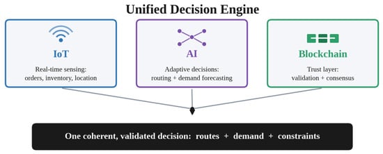
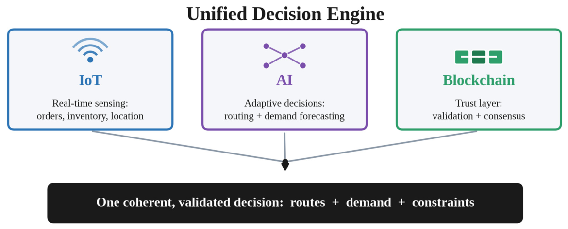
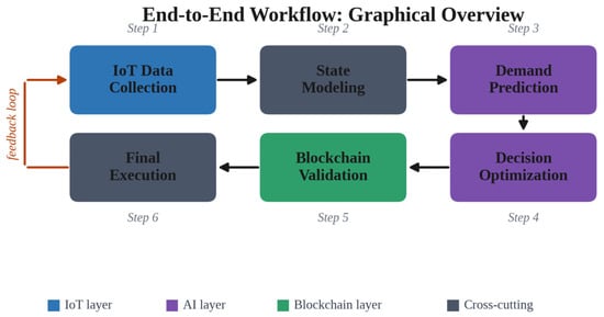
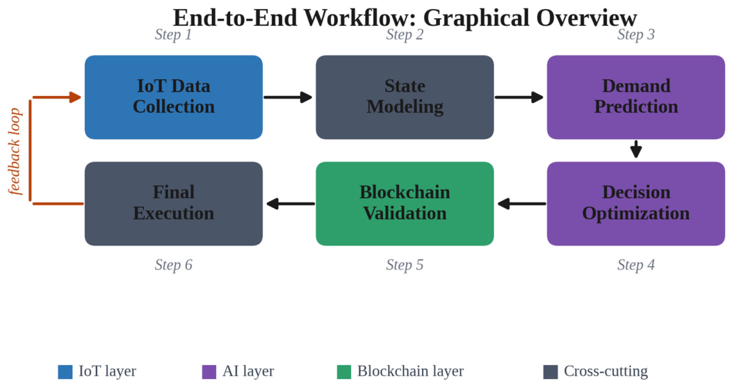
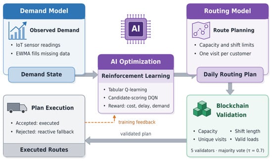
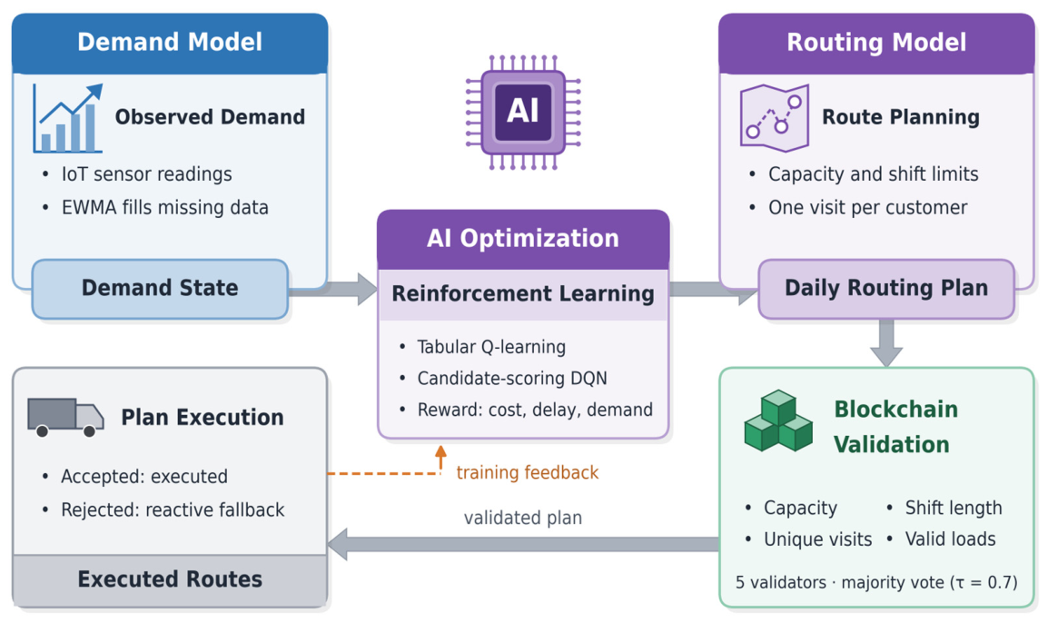
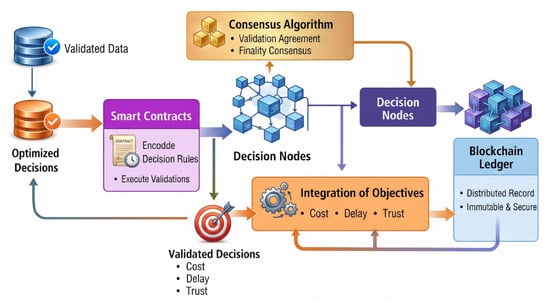
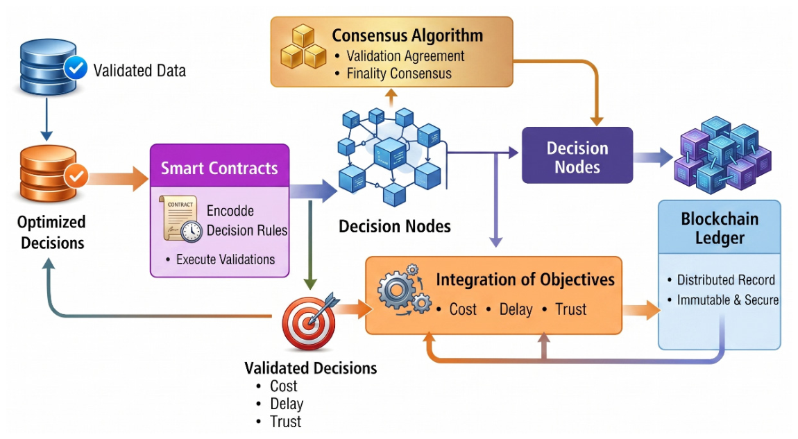
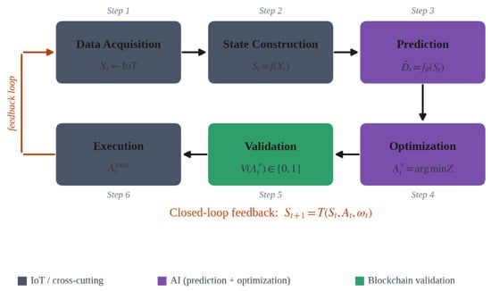
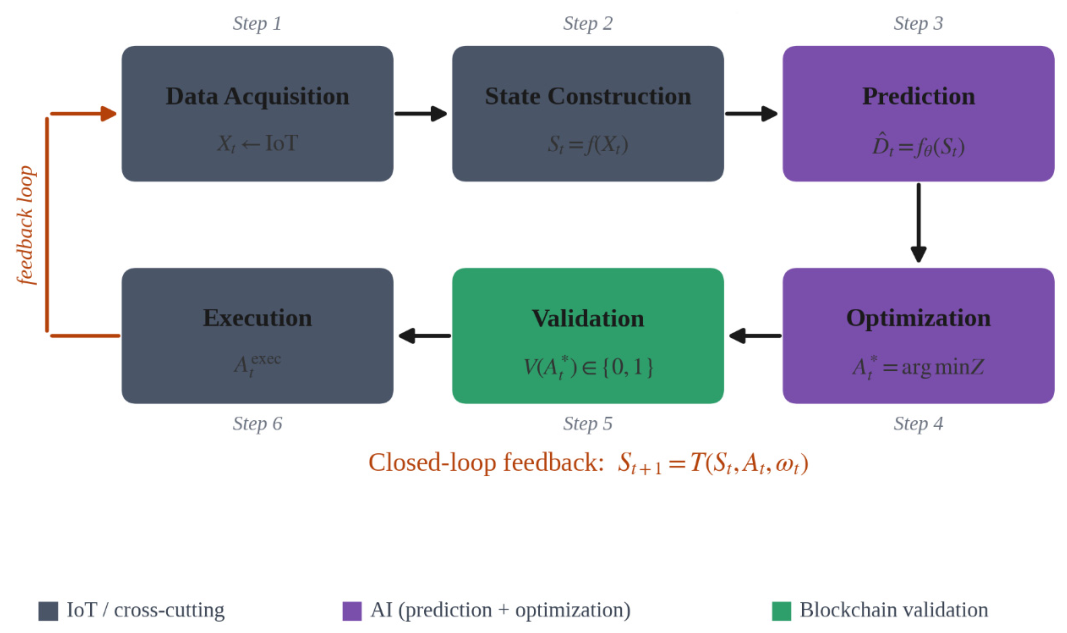
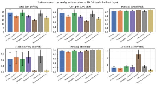
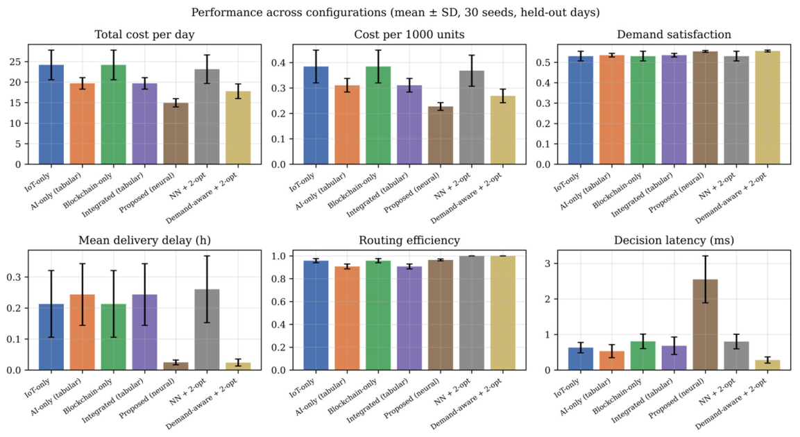
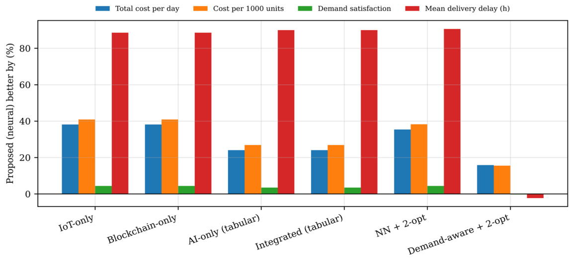
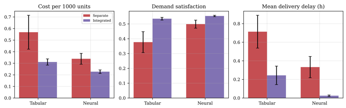
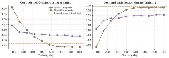
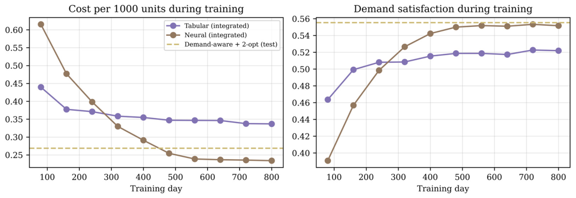
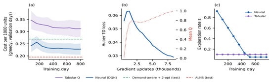
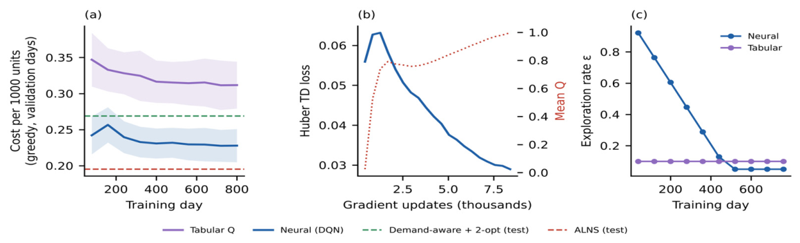
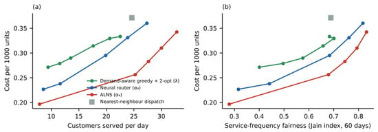
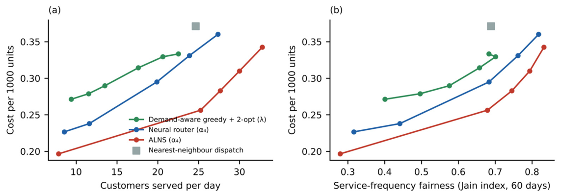
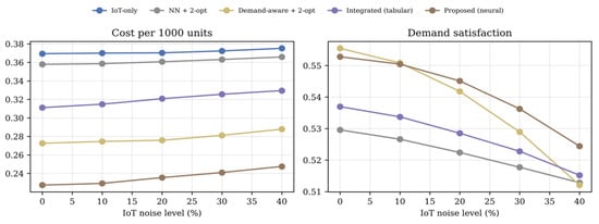
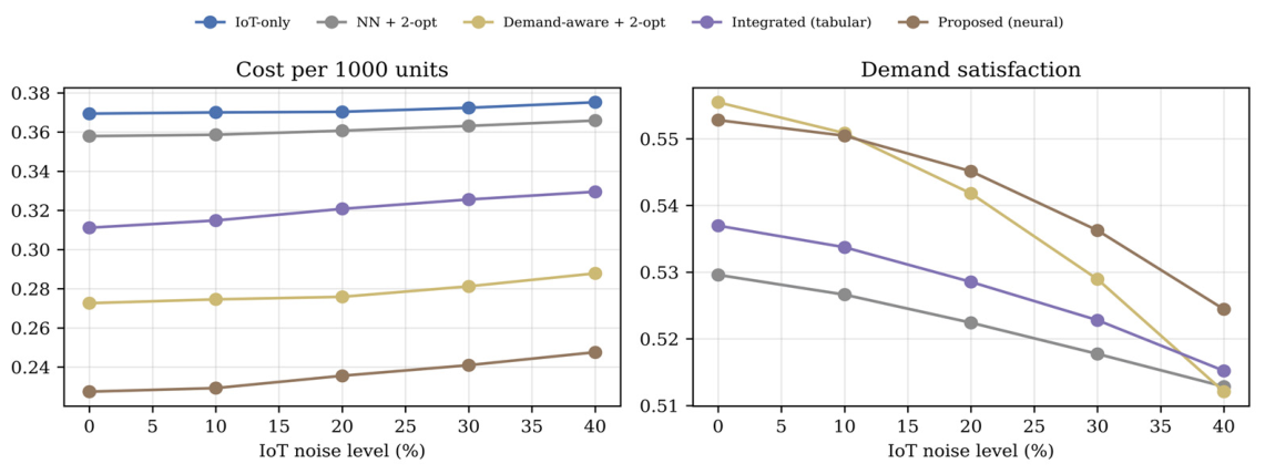
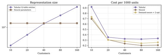
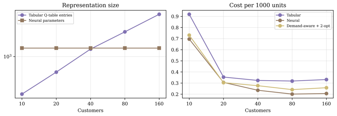
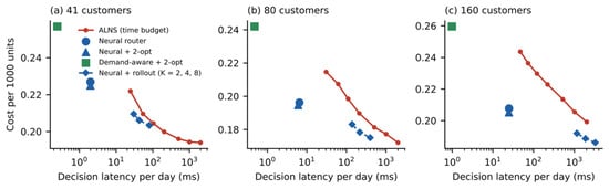
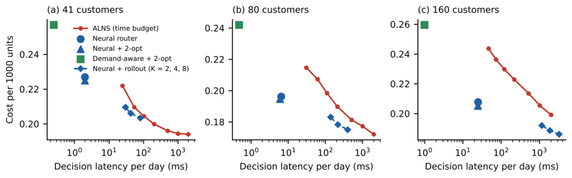
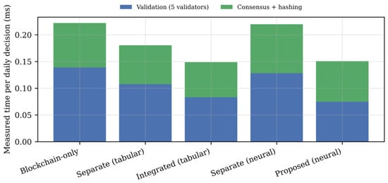
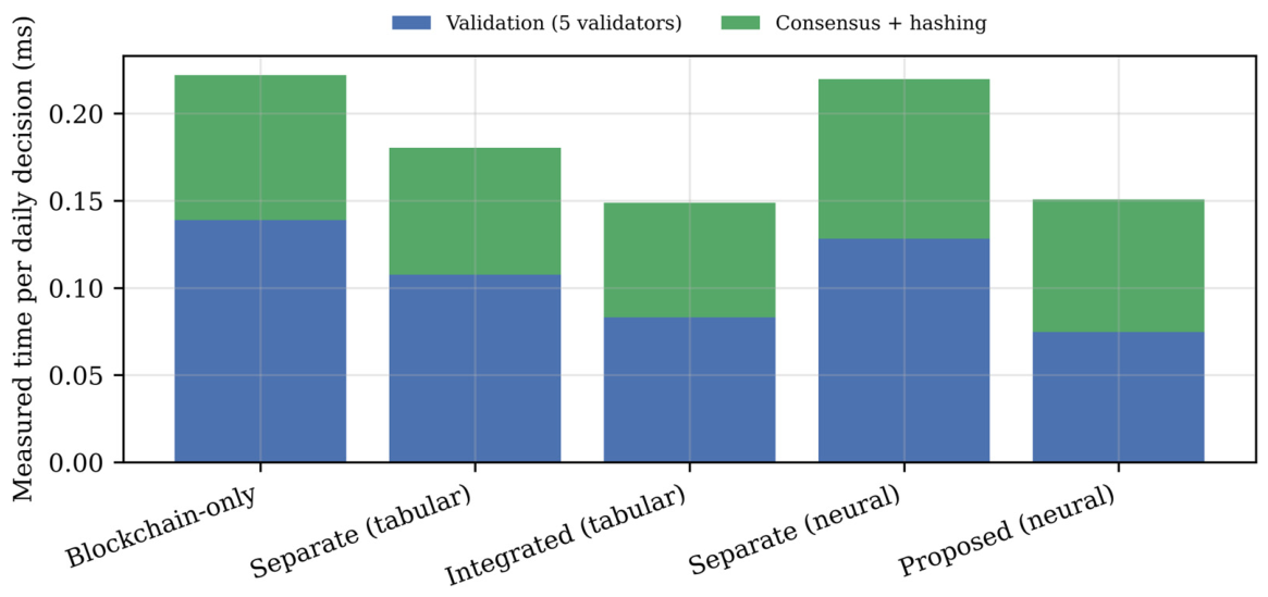

Disclaimer/Publisher’s Note: The statements, opinions and data contained in all publications are solely those of the individual author(s) and contributor(s) and not of MDPI and/or the editor(s). MDPI and/or the editor(s) disclaim responsibility for any injury to people or property resulting from any ideas, methods, instructions or products referred to in the content. |
© 2026 by the authors. Licensee MDPI, Basel, Switzerland. This article is an open access article distributed under the terms and conditions of the Creative Commons Attribution (CC BY) license.