


Abstract
Tunneling magnetoresistance (TMR) sensors are highly sensitive magnetic field detectors with applications in biomagnetic sensing and human–computer interfaces. However, the systematic optimization of TMR sensor structures and array configurations for magnetic eye tracking remains limited. This study presents a simulation-guided approach to optimize TMR sensor arrays for eye tracking. First, a finite element model of a CoFeB/MgO/CoFeB magnetic tunnel junction was developed in COMSOL Multiphysics to optimize the MgO barrier thickness. Simulations from 0.5 to 4.0 nm showed that a 1.5 nm MgO barrier achieved an MR ratio of 285%, a sensitivity of 0.13 Ω·m/A, and a wide linear sensing range. TMR arrays with three to seven sensors were then evaluated using an NdFeB magnetic marker and a spherical eyeball model. The five-sensor array achieved the highest overall performance. Elliptical (O-shape) and sinusoidal (wave-shape) eye trajectories were further simulated using time-dependent magnetic field analysis with an ALE moving mesh. The maximum value method successfully reconstructed both trajectories with good agreement with the original paths. These results demonstrate the feasibility of TMR-based wearable eye tracking for human–computer interfaces.
1. Introduction
Tunneling magnetoresistance (TMR) sensors based on magnetic tunnel junctions (MTJs) have undergone rapid development since the discovery of large TMR effects in MgO barrier junctions, achieving magnetoresistance ratios exceeding 200% at room temperature [1,2]. The fundamental mechanism relies on quantum mechanical spin-dependent tunneling through an ultrathin insulating barrier (typically MgO), where the resistance of the junction depends on the relative magnetization orientation of the two ferromagnetic electrodes [3]. CoFeB/MgO/CoFeB-based MTJs have become the industry standard due to their excellent spin filtering properties, high thermal stability, and compatibility with semiconductor fabrication processes [4,5].
The optimization of the MgO barrier thickness is critical for maximizing TMR sensor performance. The barrier thickness directly influences the tunneling probability, resistance area product, and magnetoresistance ratio. While thinner barriers reduce resistance and improve signal-to-noise ratio, excessively thin barriers lead to pinhole formation and electrical shorting; conversely, thicker barriers increase resistance beyond the optimal measurement range [6,7]. Recent studies have shown that TMR ratios can oscillate with barrier thickness due to quantum well resonance effects, and optimal thicknesses in the range of 1.0–2.0 nm have been widely reported [8,9].
TMR sensors have demonstrated picoTesla- to sub-picoTesla-level detectivity in biomagnetic sensing applications such as magnetocardiography and magnetoencephalography, offering high sensitivity without cryogenic cooling [10,11,12]. Their potential has also expanded to wearable biomedical devices, including neural sensing and human–computer interfaces [11,13]. Eye tracking is a technology of growing importance for assistive communication, virtual/augmented reality (VR/AR), neurological diagnosis, and human–computer interaction [14]. Conventional eye tracking methods based on infrared corneal reflection (pupil–corneal reflection, P-CR) are susceptible to ambient light interference and require line of sight to the eye [15]. Magnetic-based eye tracking, which uses a small permanent magnet mounted on or embedded in a contact lens together with an array of external magnetic sensors, offers a promising alternative that is insensitive to lighting conditions and can operate through closed eyelids [16,17]. More recent work has further explored magnetic tracking systems for six-degree-of-freedom (6-DoF) motion reconstruction using miniature magnet assemblies [18], and wearable magnetic eye tracking for neurological disorder prediction [19]. Tanwear et al. fabricated a proof-of-concept eyeglass frame system integrating three TMR sensors with a permanent magnet-embedded contact lens, achieving a mean gesture control accuracy of 90.8% ± 5.9% across 13 participants using a threshold-based classifier [20]. This study validated TMR sensing for eye gesture control. Its three-sensor placement (top, left, and right) limits the detectable directions and is sensitive to misalignment. For example, one sensor was misclassified in 50% of trials when a participant’s face was off-center. The authors proposed machine learning classification, not array redesign, as future work, leaving open how many sensors are needed, their placement, and the resulting trade-offs.
Recent studies have continued to expand the magnetic approach. Bevilacqua et al. demonstrated a wearable wireless magnetic eye tracker and validated it in vitro and in vivo for vestibulo-ocular reflex analysis [21]. Luo et al. developed tunneling magnetoresistance based magnetrodes with a detection limit of 300 pT/√Hz at 1 kHz and targeted the magnetic fields of neuronal spikes [22]. Soft magnetoelastic eyelid sensors have been used to decode fatigue levels from blink dynamics [23], and ferrofluid-based designs offer an alternative electromagnetic route to eye motion monitoring [24]. Skin-attached piezoelectric sensor arrays have also monitored oculomotor movements continuously [25]. These studies confirm the sensitivity of magnetic sensing at the eye. They do not address how many TMR sensors an array should contain, where the sensors should be placed, or how crosstalk and complexity trade against localization accuracy. The present work addresses this array-level optimization problem.
However, systematic finite element optimization of both MTJ structures and TMR sensor array configurations for magnetic eye tracking remains limited. Rather than relying on a single hardware configuration, we develop a coupled COMSOL Multiphysics 6.2 finite element magnetostatic model and Monte Carlo statistical simulation framework to systematically explore the TMR sensor design space for eye movement tracking. To our knowledge, this is the first study to computationally derive an optimal TMR sensor count for eyeball movement sensing, shifting the design process from trial-and-error hardware iteration toward simulation-guided optimization. Hence, in this work, we present simulations: (i) optimization of the MgO barrier thickness in a CoFeB/MgO/CoFeB MTJ using COMSOL Multiphysics; (ii) evaluation of array configurations ranging from three to seven sensors, quantifying how classification accuracy, angular resolution of gaze direction, signal-to-noise ratio, and robustness to random perturbations with sensor number and geometric arrangement. Two trajectory reconstruction methods are further compared, and the feasibility of the proposed system is assessed using elliptical (O-shape) and sinusoidal (wave-shape) eye movement trajectories [26,27].
2. Methods
2.1. MTJ Device Simulation
The MTJ device was modeled using COMSOL Multiphysics 6.2. The device geometry and material properties were defined based on standard CoFeB/MgO/CoFeB-based MTJ stacks used in TMR sensor fabrication [4]. The MTJ stack consists of nine layers from bottom to top: a copper (Cu) bottom lead (50 nm), an IrMn antiferromagnetic (AFM) pinning layer (8 nm), a CoFeB pinned layer (2 nm), a Ru spacer (0.85 nm), a CoFeB reference layer (2 nm), an MgO tunnel barrier (variable thickness), a CoFeB free layer (1.8 nm), an IrMn AFM top layer (8 nm), and a Cu top lead (50 nm). The junction cross-section is 1 μm × 1 μm, giving a total stack height of approximately 123.65 nm (for the 1 nm MgO configuration). The complete stack structure is summarized in Supplementary Materials.
Each layer was assigned appropriate electrical conductivity (σ), relative permittivity (εr), and density values, as summarized in Table 1. The MgO barrier was assigned the field-dependent effective conductivity σeff (θ) defined below, while the ferromagnetic CoFeB layers were assigned a conductivity of 2.38 × 10⁶ S/m. The copper leads use the standard annealed copper conductivity of 5.998 × 10⁷ S/m with a linearized resistivity of 1.72 × 10⁻⁸ Ω·m at a reference temperature of 298 K [28].
Table 1.
Material properties of the MTJ stack layers.
The physics interface used was Electric Currents (ec) in Stationary mode. A terminal voltage of Vapplied = 1 V was applied to the terminal boundary, with the ground defined at bottom surface. The mesh type was free tetrahedral with automatic sizing at the finest setting. A parametric sweep study was conducted with two sweep parameters: (i) external magnetic field Hext ranging from −15 to 15 kA/m in 0.3 kA/m steps for the R-H curve, and (ii) Vapplied ranging from 0 to 1 V in 0.05 V steps for the I–V characterization. The total number of solutions for the R-H sweep was 101. The MgO barrier thickness was varied parametrically across five values: 0.5, 1.0, 1.5, 2.0, and 4.0 nm. For each thickness, the resistance as a function of the external magnetic field was computed, and the MR ratio, sensitivity, and linear range (L.R.) were extracted.
The Electric Currents interface solves Ohmic conduction and does not by itself contain spin-dependent transport. We therefore couple the magnetic state of the junction into the interface through the barrier conductivity. Let θ denote the angle between the free-layer and reference-layer magnetizations. The tunnel conductance follows the Jullière form G(θ) = GP (1 + P2 cosθ)/(1 + P2), where GP is the parallel-state conductance and P ≈ 0.77 is the effective spin polarization of the CoFeB/MgO/CoFeB junction. The corresponding resistance is R(θ) = RP (1 + P2)/(1 + P2 cos θ), so that R(0) = RP and R(π) = RP (1 + P2)/(1 − P2). The magnetoresistance ratio, (RAP − RP)/RP = 2P2/(1 − P2), then evaluates to 285%, in agreement with the value extracted from the computed curves in Section 3.1. In the model, this angular dependence is assigned to the MgO domain as an effective conductivity σeff(θ) = σP (1 + P2 cos θ)/(1 + P2), with σP = d/(A ⋅ RP), where d is the barrier thickness and A = 1 μm2 is the junction area. For each thickness, σP is set by the parallel-state resistance of that configuration. For each field value of the parametric sweep, θ(Hext) follows from a macrospin equilibrium of the free layer, which minimizes the sum of the uniaxial anisotropy energy and the Zeeman energy. The reference layer is held fixed by the synthetic antiferromagnetic pinning stack. The sweep therefore maps Hext to θ, θ to σeff, and σeff to the terminal current at the applied bias of 1 V. The junction resistance R(Hext) follows from the ratio of the applied voltage to the computed terminal current.
In this model, P is thickness-independent by construction. The model therefore predicts the MR ratio at a chosen operating point. It does not predict the variation of the MR ratio with barrier thickness.
The layer thicknesses follow the standard CoFeB/MgO/CoFeB sensor stack of reference [4]. The two IrMn layers are each 8 nm thick, within the established thickness range of exchange bias layers in this stack. The 0.85 nm Ru spacer sits at the antiferromagnetic RKKY coupling peak, so the pinned and reference layers form a synthetic antiferromagnet with a near-zero net moment. The CoFeB free layer (1.8 nm) is thinner than the reference layer (2 nm), which reduces its magnetic moment and coercivity and improves its field response. The copper leads are 50 nm thick, so the lead resistance stays negligible against the junction resistance. Copper interdiffusion under post-deposition annealing is a fabrication concern. It does not enter the present model, in which copper appears only through its measured room temperature conductivity. A change in that conductivity would add only a small constant series offset to the total resistance. The MgO thicknesses studied here, 0.5 to 4.0 nm, bracket the window in which an MgO barrier is meaningful for a sensor junction. Below 0.5 nm, pinhole-mediated conduction dominates and the resistance area product approaches the lead resistance. Above 4.0 nm, the resistance area product grows exponentially with thickness and leaves the range that a wearable readout circuit can measure with an adequate signal-to-noise ratio.
The choice of this range also follows the literature on MgO barrier junctions. Yuasa and Djayaprawira reviewed how the TMR ratio and the resistance area product depend on the MgO barrier thickness in crystalline MgO (001) junctions [29]. Experimental work on sputtered CoFeB/MgO/CoFeB junctions reports the same dependence [6], including an oscillation of the TMR ratio with barrier thickness [8]. The thicknesses sampled here follow the grid used in those reports.
2.2. Multi-Sensor Combination Analysis
To evaluate the benefit of multi-sensor configurations, different combinations of TMR sensors with varying numbers of sensor were simulated. The eye tracking system estimates the two-dimensional gaze direction θ = (α, β), where α and β denote the horizontal and vertical gaze angles, respectively, from the measured TMR sensor responses. Gaze angles of ±7° to ±12° were considered to represent moderate eye rotations during gaze shifts. The dipole position is computed using full spherical rotation. In practice, the TMR readings are also affected by common-mode drift due to temperature variations and gain uncertainty in the readout electronics, as commonly observed in magnetoresistive sensor arrays [19,20]. To account for these systematic effects, the inverse problem is formulated with four unknown parameters, θ = (α, β, δoff, δscale), where α and β are the horizontal and vertical gaze angles, and δoff and δscale are the common-mode offset and gain drift, respectively. Offset and scale drift are assumed to be common to all sensors representing shared temperature effects on the TMR wafer and readout circuit. The TMR resistance change is modeled as ΔR = S·H, avoiding the tanh saturation that would compress the signal at high fields. This is appropriate for the field strengths encountered in eye tracking (~100–1000 A/m). The forward measurement model for the i-th TMR sensor is
where S = 0.13 Ω·m/A is the TMR sensitivity from previous simulation, consistent with typical values reported for modern TMR sensors based on magnetic tunnel junctions [30], Hi(α, β) is the radial magnetic field component at sensor i, εi represents additive measurement noise, and μ0 is the permeability of free space. The eye-attached magnet is modeled as a point magnetic dipole oriented along the z-axis. This is valid when the magnet dimensions are small compared to the sensor–magnet distance (~6–30 mm). The magnetic field is computed from the dipole model, following the approach used in magnetic eye tracking systems [1,4]:
where m = 1.6 × 10⁻² A·m2 is the dipole moment of the eye-attached magnet, and r is the vector from the dipole to each sensor position on a ring of radius Dsensor = 18 mm. This dipole approximation is valid when the magnet dimensions are small compared to the sensor–magnet distance, as is the case in the present configuration (~6–30 mm) [19,31].
The Jacobian matrix J∈ℝ{N×4} of the measurement model with respect to the parameter vector is
with columns corresponding to derivatives with respect to α, β, δoff, and δscale, respectively. The last two columns are J[:,2] = 1 and J[:,3] = S·Hi, which are the offset sensitivity and gain sensitivity, respectively. This Jacobian-based formulation follows the methodology established for magnetic source localization in biomedical applications [31].
The observability of the inverse problem is characterized by the singular value decomposition (SVD) of the column-normalized Jacobian Ĵ = J/‖J‖COL:
To quantitatively evaluate the spatial observability and geometric conditioning of the sensor configurations, four Jacobian-based metrics are considered. The minimum singular value (σmin) characterizes the sensitivity of the system to measurement noise, with a higher value indicating greater robustness. The condition number, defined as κ = σmax/σmin, evaluates the geometric conditioning of the sensor configuration, where a lower value indicates better conditioning and reduced sensitivity to numerical errors. The information volume, quantified by det(JTJ), is proportional to the product of the squared singular values and therefore represents the overall information content of the measurement system. Finally, the isotropy, defined as ι = σmin/σmax, describes the uniformity of sensitivity across different spatial directions, with values closer to unity indicating more uniform and direction-independent observability.
For N < 4 sensors, the system is underdetermined, with σmin tending to 0 and κ tending to ∞, rendering localization impossible. For N = 4, the system is exactly determined, making it highly sensitive to noise and unable to tolerate sensor failure. For N ≥ 5, the system becomes overdetermined, enabling noise suppression through measurement redundancy.
As the number of TMR sensors increases, the angular spacing between adjacent sensors on the mounting ring decreases, leading to measurable magnetic crosstalk. This effect is expected for closely spaced magnetic sensor arrays. Each sensor’s local bias field may leak into neighboring sensors, introducing a systematic error that cannot be removed by the inversion algorithm (which does not model crosstalk explicitly). The crosstalk is modeled as
where the coupling matrix is
with coupling strength kc = 0.10 and characteristic angular distance φ0 = 50°. This model captures the physical reality that sensors in close angular proximity experience stronger mutual interference. The inter-sensor coupling follows exponential decay with angular distance. This exponential decay model approximates the 1/r3 dipole–dipole interaction between sensor bias magnets, averaged over the ring geometry [32]. The crosstalk introduces a systematic error that grows with sensor density, creating a trade-off against the noise-averaging benefit of additional sensors.
Localization performance is evaluated via Monte Carlo (MC) simulation across N = 3 to 7 TMR sensors. For each sensor configuration, the optimal angular layout is determined by exhaustive search over all C(12, N) combinations of 12 candidate positions (at 30° intervals on the ring), maximizing a composite observability score. This combinatorial optimization approach ensures that the comparison is between the best possible configuration at each sensor count, rather than arbitrary placements.
For each relative noise level σrel, ranging from 1% to 20% of signal RMS, a MC simulation was performed to evaluate the robustness of the sensor configurations under measurement noise and parameter perturbations. At each noise level, 10 off-center gaze positions (α, β) were considered. For each gaze position, random nuisance parameters, including an offset perturbation δoff ~ N(0, σoff) and a scale perturbation δscale ~ N(0, σscale), were generated. The corresponding true sensor measurements were then calculated by incorporating both scale and offset variations as well as sensor crosstalk, according to Rtrue = Rnom·(1 + δscale) + δoff + K·Rnom. Gaussian measurement noise was subsequently added to obtain the measured response, Rmeas = Rtrue + ε, where each noise component satisfies εi ~ N(0, σrel·Rrms). The perturbed measurements were inverted using a Levenberg–Marquardt algorithm to simultaneously estimate the gaze angles (α̂, β̂), offset perturbation δ̂off, and scale perturbation δ̂scale. The localization error for each trial was calculated as e = √[(α̂ − α)2 + (β̂ − β)2], expressed in degrees. For statistical robustness, 200 independent Monte Carlo trials were performed for each gaze position, resulting in a total of 2000 samples for each noise level. The resulting localization errors were then used to calculate the mean localization error (MLE), root mean square error (RMSE), 95th-percentile localization error, and effective signal-to-noise ratio (SNR).
The Levenberg–Marquardt algorithm is used for nonlinear least squares inversion [33]. The effective SNR accounts for all noise sources:
This formulation captures the fact that crosstalk acts as an irreducible noise floor that increases with sensor count, unlike random measurement noise, which can be reduced through averaging.
A composite performance score is defined to capture the multi-dimensional trade-off between accuracy, robustness, observability, and complexity:
where tilde (~) denotes min–max normalization across all N values, and all components are listed in Table 2.
Table 2.
All components and parameters for MC simulation.
The weights encode the design priorities of a wearable device. Accuracy receives weight 1.0 because gaze error is the primary specification. Failure robustness receives 0.4 because the device must remain functional after a single sensor failure. Effective SNR and RMSE stability receive 0.3 each. Isotropy and conditioning receive 0.15 each as diagnostic measures of observability. Complexity receives 0.45 because readout channels, calibration effort, and frame form factor constrain a wearable system. The sensitivity analysis in Section 3.2 tests every weight at ± 50%.
The complexity model includes a nonlinear penalty for N > 5:
reflecting the increased cost of multi-channel readout electronics, calibration requirements, and form factor constraints for wearable applications.
C(N) = N + 0.15·N2 + 1.5·max(0, N − 5)
2.3. Eye Tracking System Model
A separate COMSOL Multiphysics model was developed to simulate the magnetic field generated by a NdFeB permanent magnet marker on an eyeball and detected by an optimized sensor array combination mounted on a glasses frame platform.
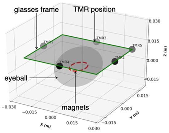
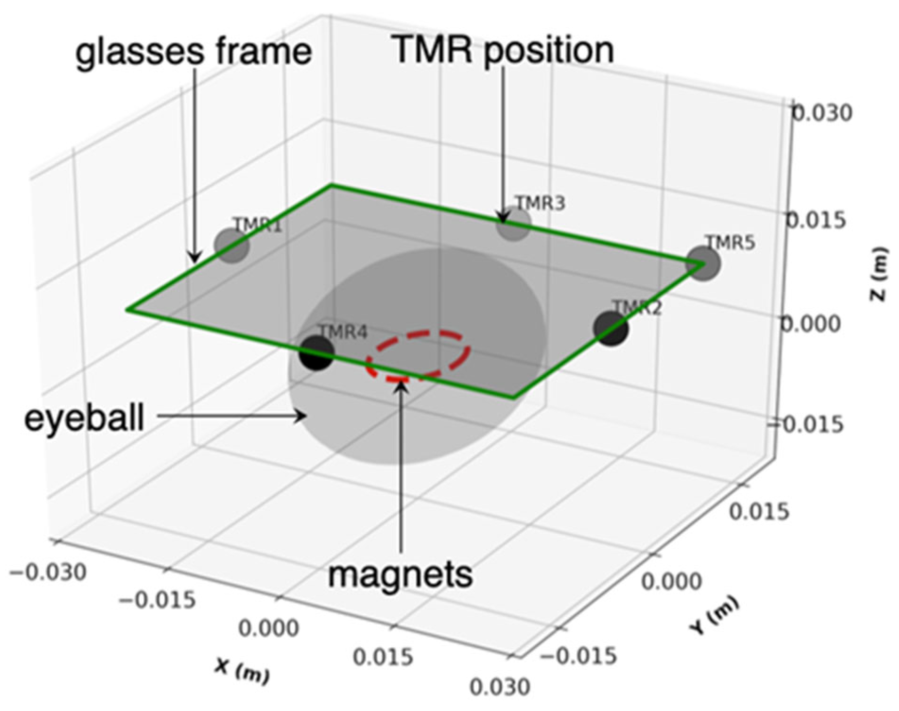
The simulation domain is a 120 × 120 × 120 mm3 air box (μr = 1, σ = 0 S/m, εr = 1) centered at the origin in Figure 1. A spherical eyeball (non-magnetic with σ = 0.5 S/m and εr = 80) model (radius Reye = 12 mm) is centered at the origin. A motion buffer shell (radius Rbuf = 16 mm) surrounds the eyeball for the arbitrary Lagrangian–Eulerian (ALE) mesh deformation. A NdFeB magnet (Br = 1.4 T, μr = 1.05, σ = 1 × 10⁶ S/m, εr = 1, magnetization direction along z-axis) ring with radius rmag = 3 mm is placed on the anterior surface of the eyeball at an initial position of (0, 0, 12) mm. The sensor plane is located at z = 22 mm, corresponding to a 10 mm gap from the magnet plane. A glasses frame plate of 50 × 30 mm2 is defined as the work plane at z = 22 mm. As the eye rotates, the magnet moves along a defined trajectory in the plane z = 12 mm, and each sensor records the local magnetic flux density B(t) as a function of time. In this model, spatial occupation-optimized TMR sensor combinations are used for eye movement tracking. A small spherical volume (radius 0.5 mm) is defined at each sensor location for mesh refinement. This section presents the complete mathematical framework, physical principles, approximations, and implementation details for both methods [32,34,35].
Figure 1.
Schematic of the eye tracking model showing the eyeball, NdFeB magnet, and five-TMR sensor array.
To implement the eye tracking simulation, two representative eyeball trajectory patterns, namely an elliptical (O-shape) trajectory and a sinusoidal (wave-shape) trajectory, were defined as the input trajectories for reconstruction by the proposed eye tracking system. The magnet position of the O-shape trajectory follows:
where the ellipse has semi-axes 5 mm (x) and 3 mm (y) and TO = 6.5 s is the period.
The magnet height is fixed at mz(t) = 12 mm during the motion, so the trajectories lie in a fixed-height plane.
The magnet position of the wave-shape trajectory follows:
where the horizontal coordinate sweeps linearly from −6 mm to +6 mm over one period Tw = 6.5 s, and the vertical coordinate oscillates with an amplitude of 2 mm at four times the sweep frequency. Here L = 6 mm is the half-range of the horizontal sweep and A = 2 mm is the vertical oscillation amplitude.
Furthermore, two magnetic flux analysis methods (time accumulation method and maximum value method) were developed to reconstruct the eyeball trajectory from the TMR sensor signals. The time accumulation method integrates the magnetic flux density signal over a defined time window to produce an accumulated magnetic flux measure.
The core principle relies on the fact that while the desired signal is deterministic and correlated with eye movement, the noise (mostly are the thermal noise in TMR sensors and the environmental interference) is stochastic and uncorrelated. Integration over time preserves the coherent signal while reducing the noise variance by a factor of 1/√M, where M is the number of samples.
The accumulated magnetic flux at sensor i over a time window [t1, t2] is defined as
In discrete form, with sampling interval Δt and M samples:
For TMR sensors with a defined sensitive axis, the accumulated flux is computed for each Cartesian component separately:
The time-dependent traces ΔRi(t) are point samples of a time-varying spatial field. To visualize how the eyeball trajectory is encoded in this field, the spatial heatmap is constructed on the sensor plane from the full-field transient solution. The time accumulation method heatmap is
In the COMSOL Multiphysics simulation, the time accumulation heatmap is implemented as a post-processing step using the time-dependent solution dataset. The integration is performed using the built-in time integration operator [35]:
where timeint is the COMSOL Multiphysics time integration operator, mf.normB is the magnetic flux density magnitude, dset is the dataset, and cpti is the Cut Point 3D dataset for sensor i.
Φacc, i = timeint(0, To, mf.normB, ‘dset’) at cpti
The maximum value method records the peak magnetic flux density observed at each sensor during the eye movement cycle. Since the B-field follows an inverse cube law with distance (B ∝ 1/d3), the maximum field at a given sensor occurs when the magnet is at its closest approach to that sensor [36]. Therefore, the maximum B-value directly encodes the extreme angular position of the eye in the direction of that sensor.
The maximum B-field magnitude at sensor i over the observation period [0, T] is
Bmax,i = maxt∈[0,T]|Bi(t)|
Similarly, the maximum of each Cartesian component:
Bmax,i,x,y,z = maxt∈[0,T]|Bi,x,y,z(t)|
In COMSOL Multiphysics, the maximum value heatmap is extracted using the time-dependent solution and the maximum operator over the solution times [35]:
where maxop is the maximum operator applied to the Cut Point 3D dataset for sensor i, evaluated across all stored time steps.
Bmax,i = maxop(mf.normB) over cpti, t ∈ [0, T]
Furthermore, for to precisely reconstruct the trajectories by maximum value method, the maximum value map is recomputed by augmenting the model with an auxiliary domain ordinary differential equation (ODE) field u(x, y, z, t) that tracks the running maximum of |Bi(t)|:
where Θ is the Heaviside step function. The positive part in Equation (24) ensures that ∂u/∂t ≥ 0 at all times. When Bi(t) rises above its previous maximum, u follows Bi(t). When Bi(t) decreases, the right-hand side vanishes and u holds its current value. The function u is therefore non-decreasing in time, and u(x, y, T) equals Bmax,i after one full trajectory period. This auxiliary equation is solved simultaneously with the Magnetic Fields and Moving Mesh problems in the same transient study. Equivalently, Bmax,i is obtained by exporting |Bi(t)| on the cut plane z at all stored time steps and evaluating the element-wise maximum in Python 3.13.
The multiple TMR signals and the heatmaps are two projections of the same magnetic field. The sensor traces are point samples of the field whose spatial envelope is visualized by Φacc, i and Bmax,i. The heatmaps therefore represent the full-field ground truth that the sensor array samples sparsely at five discrete locations; the reconstruction of the trajectory from the five discrete sensor signals is addressed in Section 3.4. The five-sensor trajectory reconstruction by Python inversion is documented in Supplementary Materials, Section S5, and its magnet path overlays are presented in Section 3.4.
Furthermore, The Magnetic Fields (mf) interface was used with a vector potential formulation and Coulomb gauge fixing (∇·A = 0) to remove the null space. Ampere’s Law was applied to all domains, with a separate Ampere’s Law node assigned to the magnet domain using the remanent flux density constitutive relation B = μ0μr(H + Hc), where Hc is derived from Br. Magnetic insulation (B·n = 0) was applied to the six outer faces of the air box. An arbitrary Lagrangian–Eulerian (ALE) Moving Mesh was applied to all domains. Prescribed displacement (dx, dy, dz) was applied to the magnet boundary to drive the mesh motion. Fixed boundary conditions (zero displacement) were applied to both the air box outer faces and the eyeball surface to constrain the mesh deformation. The mesh consisted of free tetrahedral elements with size control 0.1 mm for air/tissue domains, 0.01 mm for the magnet, and 0.2 mm for the deformation buffer zone. Laplace smoothing was used for the ALE mesh. The study was time-dependent (transient) with a time range from 0 to 10 s at Δt = 0.02 s. The PARDISO direct solver was used with strict BDF time stepping.
Two features bound the numerical error of the simulations. In the eye tracking model, the element sizes are 0.1 mm in the air and tissue domains, 0.01 mm in the magnet, and 0.2 mm in the buffer zone, with additional refinement spheres at the sensor positions. The reported fields are point values at the sensor locations, away from the magnet surface, where the field gradients are largest. In the device model of Section 2.1, the finest preset mesh resolves the 1 μm junction and its nanometer-scale layers, and the extracted resistance is a terminal integral of the conduction solution.
3. Results and Discussion
3.1. MgO Barrier Thickness Optimization
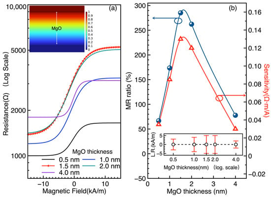
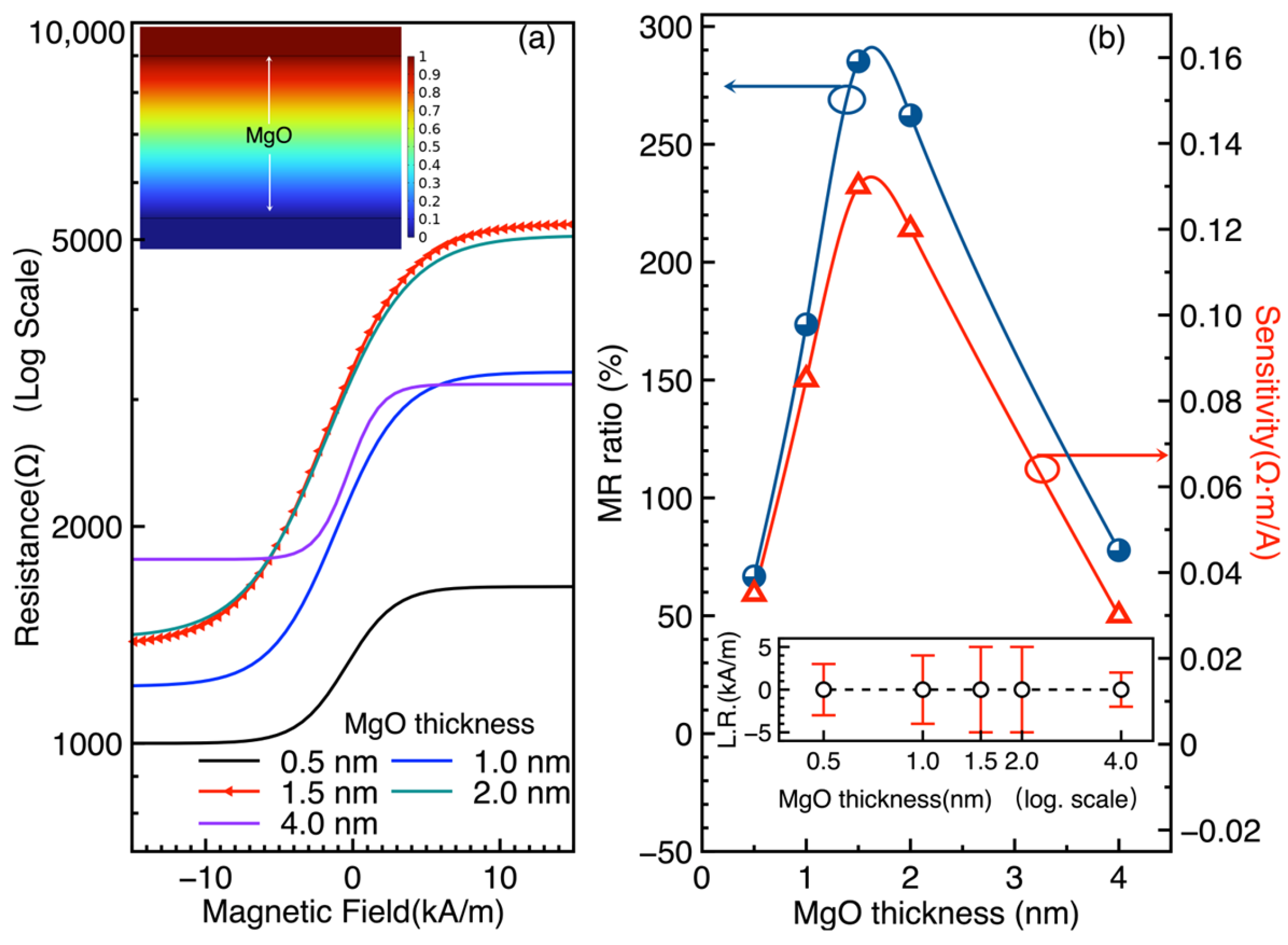
The resistance of the MTJ as a function of the external magnetic field (R-H curves) was computed for five MgO barrier thicknesses: 0.5, 1.0, 1.5, 2.0, and 4.0 nm. As shown in Figure 2a, the R-H characteristics exhibit the expected spin-valve behavior, with the resistance changing between parallel (low resistance) and antiparallel (high resistance) states as the external field sweeps from −15 to 15 kA/m. Notably, the MTJ with a 1.5 nm thick MgO layer exhibits the largest resistance variation among the investigated devices, indicating a pronounced magnetoresistive response. The MR ratio was evaluated using the following equation:
where RAP and RP are the resistances in the antiparallel and parallel states, respectively. The 1.5 nm MgO barrier yields the highest MR ratio of 285%. The sensitivity, defined as the slope of the R-H curve in the linear region, reaches 0.13 Ω·m/A for the 1.5 nm configuration. Figure 2b shows the MR ratio as a function of MgO thickness, with the inset displaying the linear range (L.R.) as a function of thickness. Both 1.5 and 2.0 nm configurations exhibit the largest linear ranges, making them suitable for analog sensing applications where a wide dynamic range is required.
Figure 2.
Effect of MgO barrier thickness on MTJ magnetoresistive performance. (a) MTJ resistance as a function of magnetic field for different MgO layer thicknesses. The inset shows the electrical potential across the MgO layer. (b) MR ratio as a function of MgO thickness. The optimal configuration is the 1.5 nm MgO MTJ with an MR ratio of 285% and sensitivity of 0.13 Ω·m/A. Inset: linear range (L.R.) as a function of thickness; 1.5 and 2.0 nm show the largest L.R.
The 285% value at 1.5 nm is consistent with the Jullière model and the Butler–Mathon theory of spin-dependent tunneling through crystalline MgO barriers [3,37]. The thickness trend in Figure 2b is extracted from the computed curves. The rising portion is consistent with the suppression of pinhole-mediated conduction at thin barriers, as reported for crystalline MgO(001) junctions [29] and sputtered CoFeB/MgO/CoFeB junctions [6]. The downturn beyond 1.5 nm is not a prediction of the constant-P model. It is consistent with the reported oscillation of TMR with barrier thickness [8]. A thickness-dependent effective polarization, which would capture interface spin filtering explicitly, is left as future work. The 1.5 nm MgO barrier is thus selected as the optimal configuration for the eye tracking TMR sensors, balancing high MR ratio, high sensitivity, and wide linear range.
Table 3 places the simulated device characteristics against experimental MgO barrier junctions. The simulated TMR ratio of 285 percent lies inside the range reported for experimental devices, which spans 88% for early epitaxial Fe/MgO/Fe junctions [1] to 604 percent for optimized CoFeB/MgO/CoFeB pseudo-spin-valves [4]. It sits above the values of standard sputtered CoFeB/MgO/CoFeB spin-valves, namely 220% [2], 230% [5], and 260% [6]. This position is expected for an idealized coherent tunneling model that omits interface disorder, roughness, and finite temperature smearing. At the sensor level, reported TMR biomagnetic sensors reach sub-picoTesla detectivity [12], and magnetrodes reach 300 pT/√Hz at 1 kHz [22]. The device parameters obtained here are compatible with that device class. The omissions listed above define the gap that experimental validation must close.
Table 3.
Comparison of the simulated TMR ratio with experimental MgO barrier junctions.
3.2. Optimization of TMR Sensor Number for Gaze Localization
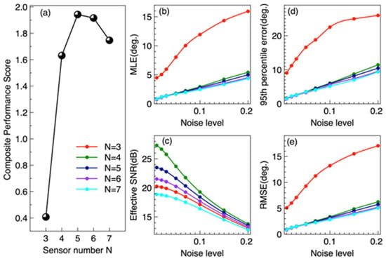
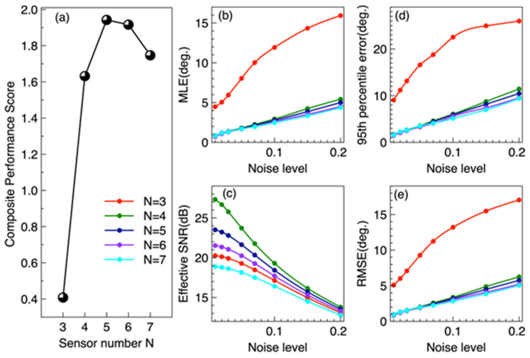
In Figure 3a, the composite performance score reaches a maximum of 1.942 at N = 5, which is close to N = 6 with 1.916, indicating that the five-sensor configuration provides the best overall performance. When N decreases from 4 to 3, the composite performance score drops sharply, because the failure robustness becomes zero (see Table 4). The MLE of N = 3 at ~8° which is separated from N = 4–7 cluster at 1.7–1.8°. N = 5 and N = 6 are nearly indistinguishable at low noise in Figure 3b. Figure 3c shows that N = 4 achieves the highest effective SNR under low-noise conditions without crosstalk; however, N = 5 maintains a higher SNR than N = 6–7 across all noise levels, owing to its lower crosstalk. Figure 3d is the 95th-percentile error, which follows a trend similar to that of the MLE in Figure 3b. The RMSE in Figure 3e shows a trend like that of MLE in Figure 3b but is more sensitive to large localization errors. At a noise level of 5%, the RMSE for N = 3 reaches approximately 9°. Table 4 summarizes the performance metrics at 5% relative noise level. The five-TMR configuration achieves the highest composite performance score (𝕊 = 1.942), representing the optimal trade-off across all evaluation dimensions.
Figure 3.
Composite performance score and performance metrics for multiple-sensor configurations. (a) shows composite performance score of the multiple-sensor combinations. (b) shows the mean localization error (MLE) of the multiple-sensor configurations as a function of noise level. (c) presents the effective signal-to-noise ratio (SNR) as a function of noise level. (d) shows the 95th-percentile error as a function of noise level. (e) presents the root mean square error (RMSE) as a function of noise level.
Table 4.
Performance comparison of TMR sensor configurations (5% relative noise).
Table 4 reveals three distinct regimes. In the underdetermined regime (N = 3), only three sensors for four unknown parameters, the Jacobian is rank-deficient (σmin = 0, condition number ~ 1015). The Levenberg–Marquardt solver produces large errors (~8°) with high variance, confirming that three TMR sensors provide insufficient spatial constraints for reliable 2D gaze localization. The system cannot resolve gaze direction and nuisance parameters simultaneously.
In the exactly determined regime (N = 4), four sensors provide exactly four equations for four unknowns, making the system solvable. However, the zero redundancy means that (i) measurement noise cannot be averaged out, and (ii) failure of any single sensor renders the system underdetermined (failure error = 90°). The condition number κ = 189 indicates moderate geometric sensitivity to noise, consistent with observations in magnetoresistive sensing systems [19,33]. This configuration is highly fragile, and it cannot average measurement noise, and any single sensor failure collapses the system.
In the overdetermined regime (N ≥ 5), the five-sensor configuration introduces the first measurement redundancy (N − 4 = 1), enabling noise suppression through least squares averaging. The MLE decreases to 1.75°, and critically, the system can tolerate a single sensor failure (failure error = 1.92° vs. 90° for N = 4). The composite performance score reaches its maximum 𝕊 = 1.942, and improved conditioning of the inverse problem. The additional spatial constraint from the fifth sensor breaks geometric symmetries present in four-sensor layouts, improving observability of the 2D gaze position.
Further increasing to N = 6 yields a marginal accuracy improvement (1.67° vs. 1.75°, a 4.6% reduction), but the inter-sensor crosstalk increases the effective noise floor (SNR drops from 21.6 to 20.2 dB), and the hardware complexity rises significantly. The composite score 1.916 is slightly lower than that of N = 5. At N = 7, the effective SNR drops to 18.1 dB, and the mean error increases from 1.67° to 1.70° compared to N = 6, demonstrating that the crosstalk penalty exceeds the noise-averaging benefit. The composite score drops to 1.747. This phenomenon is consistent with crosstalk analysis in circular magnetic sensor arrays [32]. Therefore, within the candidate layouts, noise levels, crosstalk model, and scoring weights considered in this study, five TMR sensors represent the optimal configuration for magnetic eye tracking, achieving the best overall balance among localization performance, system robustness, tolerance of a single-sensor failure, and hardware practicality. In the eye tracking context, the spatial diversity of the five-sensor array (left, right, up, down, and diagonal) captures complementary information about the magnet’s 3D position, enabling robust 2D trajectory reconstruction.
N = 5 and N = 6 are nearly tied on accuracy. The 0.08° mean error gap is about 1.6 times the Monte Carlo standard error of 0.05°. The decision for N = 5 therefore rests on robustness and complexity, not on a claimed accuracy superiority.
We further tested how strongly the optimum depends on the scoring weights of Equation (8) and the complexity model of Equation (9). Using the component metrics of Table 4, we varied each weight in turn by ±50 percent and recomputed the composite score for N = 3 to 7. The five-sensor configuration remains optimal under every single-weight variation except the complexity weight. If the complexity weight ω7 falls below approximately 0.12, the six-sensor configuration becomes marginally better, because it has the lowest mean error and condition number. Two further arguments do not depend on the weights. First, five sensors form the smallest configuration that tolerates a single-sensor failure: the failure error drops from 90° at N = 4 to 1.92° at N = 5. Second, for N ≥ 6 the inter-sensor crosstalk lowers the effective signal-to-noise ratio monotonically, from 21.6 dB at N = 5 to 20.2 dB at N = 6 and 18.1 dB at N = 7. We therefore retain five sensors as the optimum under the stated weights, and we note that it is in any case the smallest failure-tolerant configuration. The Monte Carlo estimates use 200 trials at each of 10 gaze positions, giving 2000 samples per noise level. The standard error of the reported mean localization error is therefore approximately 0.05°, far below the differences between configurations.
3.3. Spatial Magnetic Field During Eyeball Movement
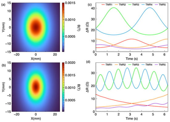
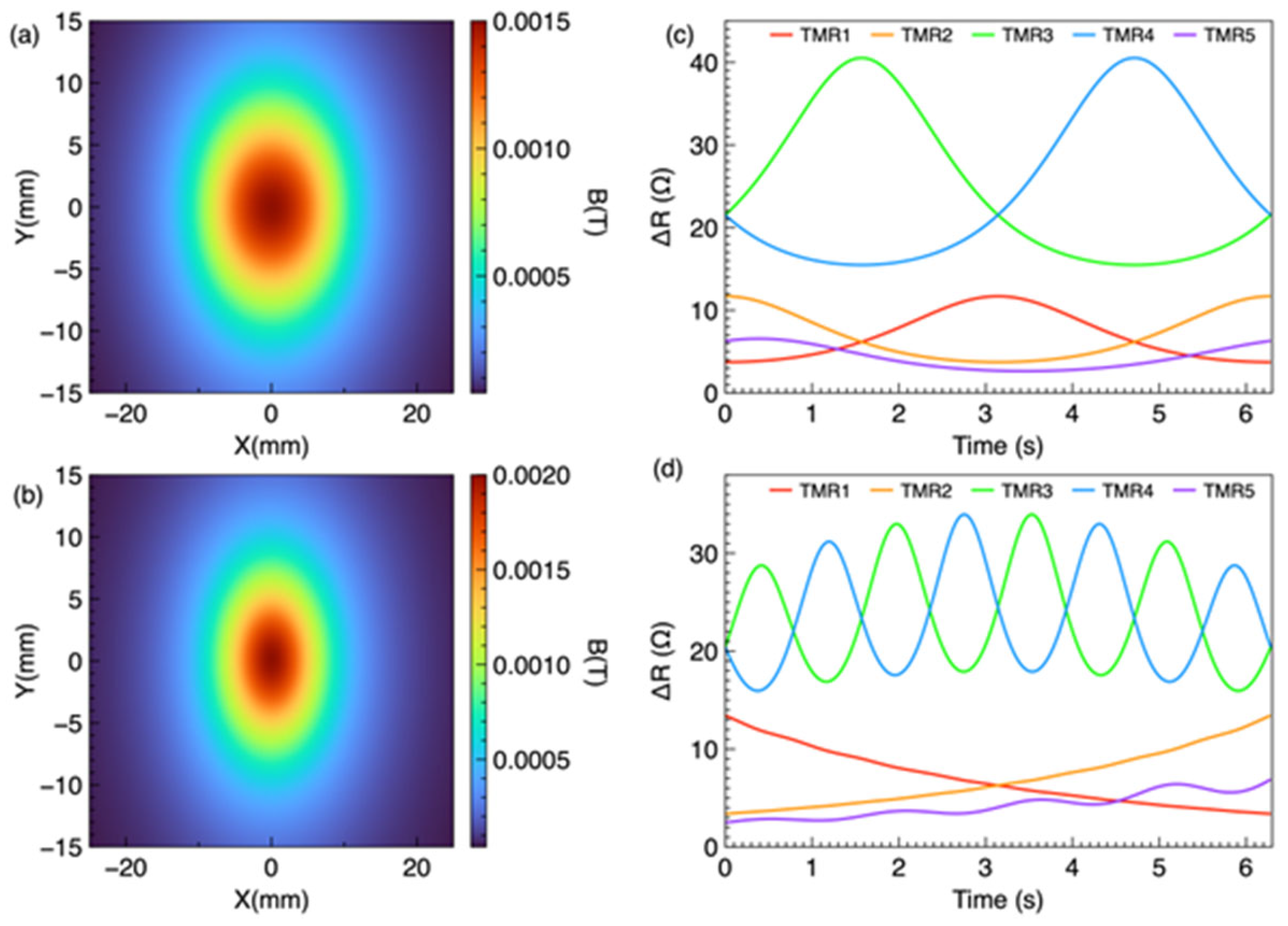
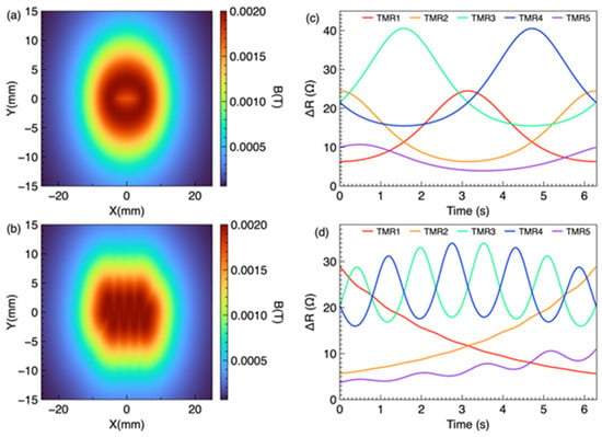
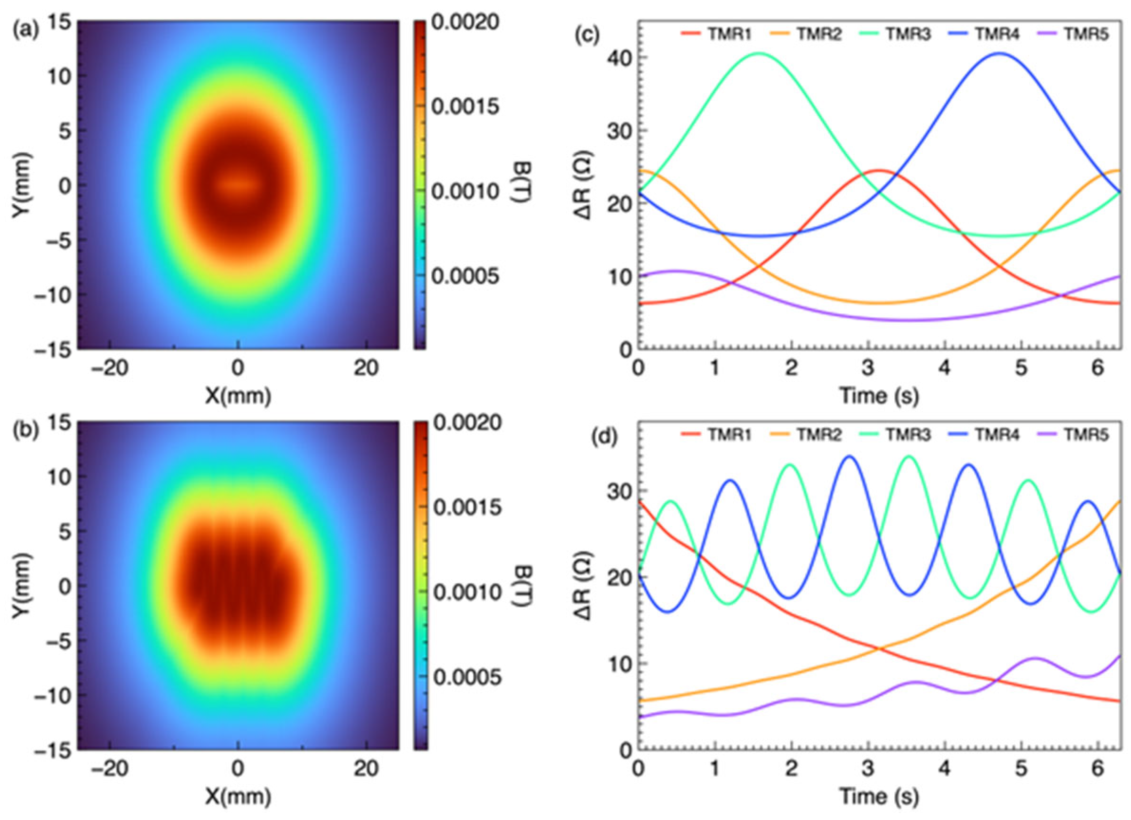
Both maps were evaluated on the sensor plane z = 22 mm over the 50 × 30 mm2 frame area. The O-shape and wave-shape trajectories were simulated separately, and the same post-processing procedure was applied to both. The time accumulation heatmap (Equation (19)) integrates the instantaneous field over one full trajectory period, whereas the maximum value heatmap (Equation (22)) retains the peak field at each spatial location, which corresponds to the closest approach of the magnet to that point and therefore encodes the spatial envelope of the trajectory. Figure 4a,b show the spatial magnetic field distributions during O-shape and wave-shape eyeball movements, respectively. In both cases, the accumulated spatial magnetic field does not visually reveal the trajectory in Figure 4a, and the wave shape cannot be visually identified in Figure 4b. This is because the magnet moves continuously, and the time accumulation method superimposes the instantaneous field distributions at all time steps, causing the spatial features to overlap and blur.
Figure 4.
Time accumulation method for sensing of O-shaped and wave-shaped eyeball movements. (a) Spatial distribution of the time-accumulated magnetic flux density on the sensor plane during O-shaped eyeball movement, which does not directly reproduce the O-shaped trajectory. (b) Spatial distribution of the time-accumulated magnetic flux density on the sensor plane during wave-shaped eyeball movement, which does not directly reproduce the wave-shaped trajectory. (c) Responses of the five TMR sensors during O-shaped eyeball movement. (d) Time-accumulated responses of the five TMR sensors during wave-shaped eyeball movement, enabling identification and reconstruction of the underlying trajectory.
Figure 4c,d show the individual TMR sensor responses (B-field magnitude) during the O-shape and wave-shape trajectories, respectively. Each sensor exhibits a distinct temporal signature depending on its spatial position relative to the moving magnet. The temporal patterns reflect the periodic nature of the trajectories, with the O-shape producing a single-frequency response and the wave-shape producing a more complex multi-frequency response due to the vertical oscillation at four times the sweep frequency.
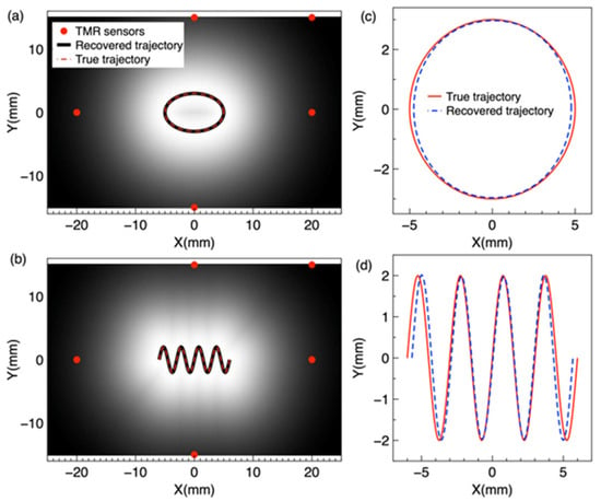
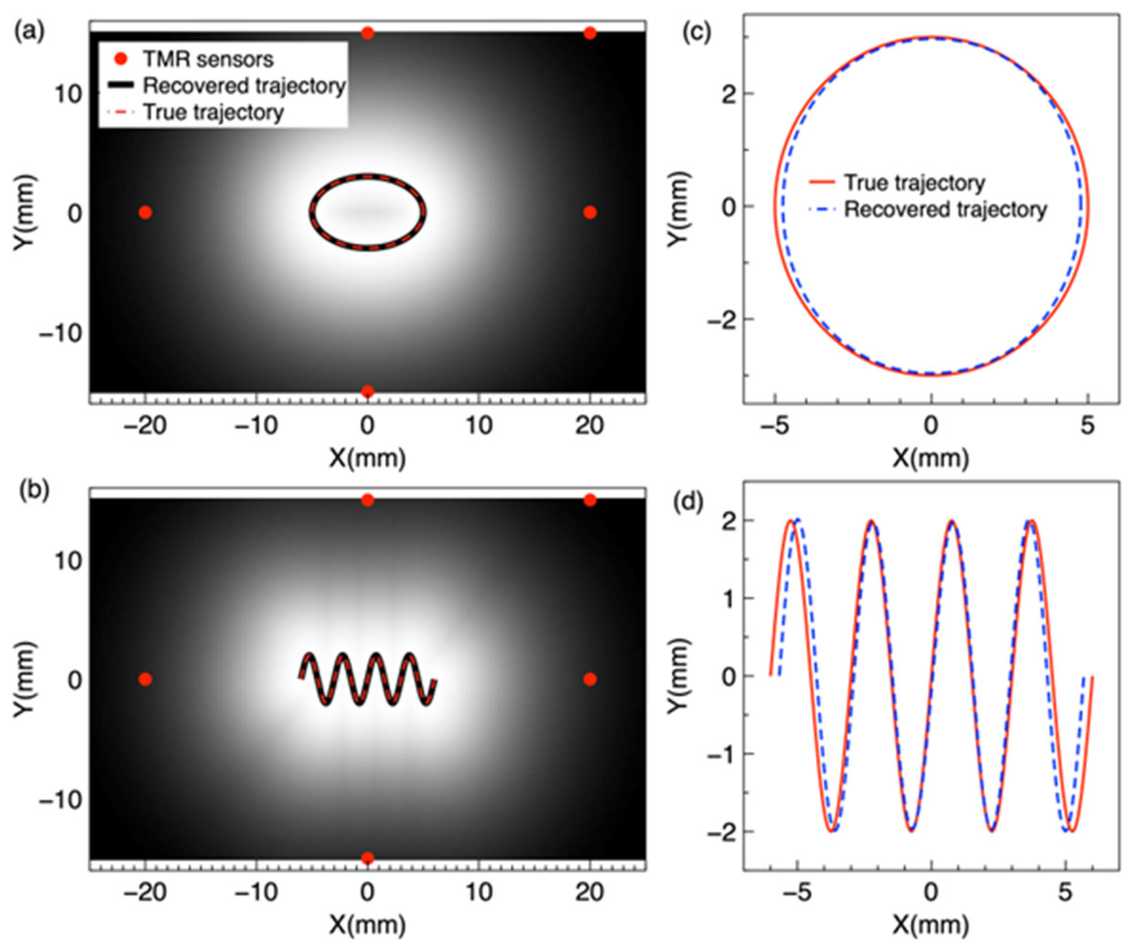
In the maximum value method, the peak magnetic field magnitude at each spatial point over the trajectory period is retained to construct a map of peak field values. Figure 5a,b are rendered from the five-sensor reconstruction: each ΔR trace is converted to field through Equation (1), the five traces are inverted to the marker trajectory (Section 3.4; Supplementary Section S5), and the peak field map (Equations (2), (21) and (22)) is evaluated from the reconstructed positions on the sensor plane grid. This method preserves the spatial envelope of the trajectory because each point on the trajectory corresponds to the magnet’s closest approach, yielding the highest local field. The trajectory is then extracted by identifying the locus of maximum field values.
Figure 5.
Maximum value method for sensing of O-shaped and wave-shaped eyeball movements. (a) Spatial distribution of the maximum magnetic flux density over one trajectory period on the sensor plane during O-shaped eyeball movement, which directly reproduces the O-shaped trajectory. (b) Spatial distribution of the maximum magnetic flux density over one trajectory period on the sensor plane during wave-shaped eyeball movement, which directly reproduces the wave-shaped trajectory. (c) Responses of the five TMR sensors during O-shaped eyeball movement. (d) Responses of the five TMR sensors during wave shaped eyeball movement, enabling identification and reconstruction of the underlying trajectory.
Figure 5a,b show the spatial magnetic field distributions using the maximum value method for O-shape and wave shape trajectories, respectively. In contrast to the time accumulation method, the maximum value heatmap clearly reveals the trajectory shape: the O-shape is visually identifiable as a ring pattern in Figure 5a, and the wave shape is visible in Figure 5b. This is because the maximum value method preserves the peak field at each spatial location, which corresponds to the magnet’s closest approach to that point, thereby encoding the trajectory envelope. Figure 5c,d show the corresponding five-TMR sensor responses using the maximum value method for the O-shape and wave-shape trajectories. The sensor responses are similar in temporal form to those obtained with the time accumulation method, as both methods use the same raw sensor data; the difference lies in the spatial processing of the magnetic field distribution.
The peak field maps of Figure 5a,b are evaluated on the sensor plane over one trajectory period, with the marker moving in the plane z = 12 mm. The maps are built from the five traces only, whereas the COMSOL Multiphysics full-field solution is computed independently of the inversion. The two agree with a correlation of 0.9998 for the O-shape trajectory and 0.9997 for the wave-shape trajectory, up to a uniform scale factor of 0.63 that reflects the effective dipole moment of the modeled marker. This shows that five discrete sensors retain the spatial information of the full-field distribution.
3.4. Trajectory Reconstruction
The maximum value maps of Figure 5a,b encode each trajectory as the locus of peak field values on the sensor plane: at every point, the maximum field over one period occurs at the magnet’s closest approach, so the ridge of the map traces the trajectory. Figure 6a shows the O-shape trajectory extracted from the maximum value map (black curve) overlaid on the true trajectory (red dashed curve). The red dots indicate the five TMR sensor positions. The extracted trajectory follows the true ellipse closely, confirming that the maximum value map preserves the spatial envelope of the trajectory.
Figure 6.
Reconstruction of O-shaped and wave-shaped eye movement trajectories. (a) O-shape trajectory from the maximum value method: the black curve is the trajectory extracted from the maximum value map, the red dashed curve is the true trajectory, and the red dots indicate the five TMR sensor positions. (b) Wave-shape trajectory from the maximum value method, with the same scheme as (a). (c) O-shape trajectory from the five-sensor inversion in magnet path coordinates: the blue dashed curve is the reconstructed trajectory from the five sensor signals only, and the red solid curve is the true trajectory. (d) Wave-shape trajectory from the five-sensor inversion, with the same scheme as (c).
Figure 6b shows the wave-shape trajectory from the maximum value method. The extracted wave pattern closely follows the true trajectory, including all four oscillations, confirming that the displayed peak field map preserves the shape of complex non-circular trajectories. The key advantage of this method over the time accumulation approach is that the maximum value map displays the spatial envelope of the trajectory directly, without further signal processing.
Figure 6c,d show the same two trajectories reconstructed from the five sensor signals alone, by the Python inversion documented in Supplementary Section S5. For the O-shape trajectory, the reconstructed curve (blue dashed) follows the true trajectory (red solid) over the full ellipse; for the wave-shape trajectory, it follows all four oscillations.
Figure 6a,b show the trajectory read off the ridge of the peak field map rendered from the five-sensor reconstruction, and Figure 6c,d plot the same reconstruction directly in magnet path coordinates. The ridge coincides with the reconstructed trajectory by construction, so the comparison shows what the displayed map carries: read from the map, the path deviates from the true trajectory by 0.16 mm (O-shape) and 0.33 mm (wave-shape) on average, i.e., the heatmap that a wearable system would display reproduces the trajectory quantitatively.
To verify that the trajectory can be recovered from the five sensor signals alone, the five sensor signals were converted from field to resistance and inverted step by step with the Section 2.2 dipole model and the Levenberg–Marquardt algorithm, without using any full-field data (Supplementary Materials, Section S5). For the O-shape trajectory, the reconstructed trajectory deviates from the true trajectory by 0.57 degrees on average and 1.03 degrees at most (mean position deviation 0.13 mm, maximum 0.25 mm). For the wave-shape trajectory, the deviation is 0.54 degrees on average and 1.27 degrees at most (mean position deviation 0.13 mm, maximum 0.33 mm). These results confirm that the five-sensor array alone reconstructs both trajectories. Rendering the same peak field maps from the positions recovered by the inversion reproduces the COMSOL Multiphysics full-field reference maps (Section 3.3), and the inversion agrees with the true trajectories as quantified above. Together these two comparisons show that the five traces carry the spatial information of the full field and that the reconstruction is accurate in position.
The maximum value method therefore provides a compact, image-like readout of the reconstruction, obtained by accumulating the peak field on the sensor plane; reading the path from the map requires no optimization beyond the inversion that produced it. Previous magnetic eye tracking studies have relied on dipole model inversion [18,20], and extended Kalman filtering has been applied to magnetic tracking in surgical scenes [38]. Presenting the reconstruction as a peak field map gives an intuitive spatial display for a wearable system, at the cost of the finite grid resolution of the map.
Several limitations should be acknowledged. First, this study is based entirely on COMSOL Multiphysics finite element and MC simulations; therefore, experimental validation with fabricated TMR sensors and physical eye models is needed in future studies. Second, the eyeball was modeled as a simplified sphere without surrounding anatomical structures, such as eyelid and orbit, which may alter the magnetic field distribution under practical conditions. Third, the sensor spacing and magnet size may need optimization to accommodate variations in eye size and glass frame geometry. Although measurement noise, common-mode drift, gain uncertainty, and sensor crosstalk were incorporated into the simulations, their actual magnitudes and characteristics should be experimentally quantified in future studies. Finally, the integration of the TMR sensor array with readout electronics and wireless data transmission will be necessary to develop for a complete wearable system.
4. Conclusions
This study demonstrates the feasibility of TMR-based magnetic eye tracking through systematic COMSOL Multiphysics simulation. A 1.5 nm MgO barrier in a CoFeB/MgO/CoFeB MTJ achieves an MR ratio of 285%, sensitivity of 0.13 Ω·m/A, and one of the largest linear range among the tested configurations (0.5–4.0 nm), providing the best overall magnetoresistive performance for the proposed eye tracking system. We also optimized the multiple TMR sensor configuration by MC simulation. Our results show a non-monotonic relationship between the number of sensors and system performance. Increasing the number of TMR sensors from three to five provides the largest improvement in eyeball movement and angular resolution. This improvement is mainly due to reduced ambiguity between adjacent directions and better tolerance to sensor–eye misalignment. When more than five sensors are used, the performance improvement becomes limited. In addition, inter-sensor magnetic crosstalk, reduced spatial discrimination, and increased circuit complexity. The maximum value heatmaps rendered from the five-sensor reconstruction display both the elliptical (O-shape) and sinusoidal (wave-shape) eyeball trajectories, while the time accumulation method fails to visually reveal the trajectory shape. The displayed trajectories agree with the original paths to 0.16 mm and 0.33 mm on average, showing that a five-TMR sensor array with a peak field readout is a viable approach for wearable eye tracking systems. The five-sensor inversion recovers both trajectories, with mean deviations of 0.57 degrees for the O-shape trajectory and 0.54 degrees for the wave-shape trajectory, confirming that the trajectory information is carried by the five signals alone. These results provide a simulation-based foundation for the development of TMR-based wearable eye tracking devices and support their potential applications in human–computer interfaces, clinical assessment, and assistive technologies. Future work will focus on experimental validation, further miniaturization of the sensor array and associated electronics, and integration into a wearable eye tracking platform.
Supplementary Materials
The following supporting information can be downloaded at: https://www.mdpi.com/article/10.3390/bios16110626/s1, Table S1: MTJ device geometry parameters used for the COMSOL Multiphysics simulation; Table S2: Material properties used for the COMSOL Multiphysics simulation; Table S3: Simulation setup in COMSOL Multiphysics; Table S4: Five-TMR eye tracking model parameters in COMSOL Multiphysics; Table S5: Five-sensor reconstruction errors; Figure S1: O-shape trajectory reconstruction; Figure S2: Wave-shape trajectory reconstruction.
Author Contributions
Conceptualization, P.W. and J.L.; methodology, P.W.; software, P.W.; validation, P.W.; formal analysis, J.L.; investigation, P.W.; data curation, W.W.; writing—original draft preparation, P.W.; writing—review and editing, W.W., J.L.; supervision, P.W.; project administration, P.W.; funding acquisition, P.W. All authors have read and agreed to the published version of the manuscript.
Funding
This research was funded by the Jiaxing Municipal Science and Technology Program, Proof-of-Concept Special Project, grant number 2026CGZ019.
Institutional Review Board Statement
Not applicable.
Informed Consent Statement
Not applicable.
Data Availability Statement
The original contributions presented in this study are included in the article/Supplementary Materials. Further inquiries can be directed to the corresponding authors.
Acknowledgments
The authors thank Tao Wu of ShanghaiTech University for providing access to COMSOL Multiphysics 6.2 and other equipment used in this study. During the preparation of this manuscript, the authors used ChatGPT 5.6 luna for English language editing. The authors have reviewed and edited the output and take full responsibility for the content of this publication.
Conflicts of Interest
P.W. serves as Chief Scientist of Shanghai Quantuno Hi-Tech Co., Ltd. The company had no role in the design of the study; in the collection, analyses, or interpretation of data; in the writing of the manuscript; or in the decision to publish the results. The other authors declare no conflicts of interest.
Abbreviations
The following abbreviations are used in this manuscript:
| TMR | Tunneling magnetoresistance |
| MTJ | Magnetic tunnel junction |
| MR | Magnetoresistance |
| ALE | Arbitrary Lagrangian–Eulerian |
| VR/AR | Virtual/augmented reality |
| P-CR | Pupil–corneal reflection |
| DoF | Degree of freedom |
| AFM | Antiferromagnetic |
| L.R. | Linear range |
| SVD | Singular value decomposition |
| MC | Monte Carlo |
| RMS | Root mean square |
| MLE | Mean localization error |
| RMSE | Root mean square error |
| SNR | Signal-to-noise ratio |
| ODE | Ordinary differential equation |
References
- Yuasa, S.; Nagahama, T.; Fukushima, A.; Suzuki, Y.; Ando, K. Giant room-temperature magnetoresistance in single-crystal Fe/MgO/Fe magnetic tunnel junctions. Nat. Mater. 2004, 3, 868–871. [Google Scholar] [CrossRef] [Scilit]
- Parkin, S.S.P.; Kaiser, C.; Panchula, A.; Rice, P.M.; Hughes, B.; Samant, M.; Yang, S.-H. Giant tunnelling magnetoresistance at room temperature with MgO (100) tunnel barriers. Nat. Mater. 2004, 3, 862–867. [Google Scholar] [CrossRef] [Scilit]
- Julliere, M. Tunneling between ferromagnetic films. Phys. Lett. A 1975, 54, 225–226. [Google Scholar] [CrossRef] [Scilit]
- Ikeda, S.; Hayakawa, J.; Ashizawa, Y.; Lee, Y.M.; Miura, K.; Hasegawa, H.; Tsunoda, M.; Matsukura, F.; Ohno, H. Tunnel magnetoresistance of 604% at 300 K by suppression of Ta diffusion in CoFeB∕MgO∕CoFeB pseudo-spin-valves annealed at high temperature. Appl. Phys. Lett. 2008, 93, 082508. [Google Scholar] [CrossRef] [Scilit]
- Djayaprawira, D.D.; Tsunekawa, K.; Nagai, M.; Maehara, H.; Yamagata, S.; Watanabe, N.; Yuasa, S.; Suzuki, Y.; Ando, K. 230% room-temperature magnetoresistance in CoFeB∕MgO∕CoFeB magnetic tunnel junctions. Appl. Phys. Lett. 2005, 86, 092502. [Google Scholar] [CrossRef] [Scilit]
- Hayakawa, J.; Ikeda, S.; Matsukura, F.; Takahashi, H.; Ohno, H. Dependence of Giant Tunnel Magnetoresistance of Sputtered CoFeB/MgO/CoFeB Magnetic Tunnel Junctions on MgO Barrier Thickness and Annealing Temperature. Jpn. J. Appl. Phys. 2005, 44, L587–L589. [Google Scholar] [CrossRef] [Scilit]
- Tsunekawa, K.; Djayaprawira, D.D.; Nagai, M.; Maehara, H.; Yamagata, S.; Watanabe, N.; Yuasa, S.; Suzuki, Y.; Ando, K. Giant tunneling magnetoresistance effect in low-resistance CoFeB∕MgO(001)∕CoFeB magnetic tunnel junctions for read-head applications. Appl. Phys. Lett. 2005, 87, 072503. [Google Scholar] [CrossRef] [Scilit]
- Matsumoto, R.; Fukushima, A.; Nagahama, T.; Suzuki, Y.; Ando, K.; Yuasa, S. Oscillation of giant tunneling magnetoresistance with respect to tunneling barrier thickness in fully epitaxial Fe∕MgO∕Fe magnetic tunnel junctions. Appl. Phys. Lett. 2007, 90, 252506. [Google Scholar] [CrossRef] [Scilit]
- Nozaki, T.; Hirohata, A.; Tezuka, N.; Sugimoto, S.; Inomata, K. Bias voltage effect on tunnel magnetoresistance in fully epitaxial MgO double-barrier magnetic tunnel junctions. Appl. Phys. Lett. 2005, 86, 082501. [Google Scholar] [CrossRef] [Scilit]
- Jiao, X.; Zhang, S.; Chen, C. Design of Biological Weak Magnetic Field Detection System Based on TMR Sensor. In The Proceedings of the 2023 International Conference on Wireless Power Transfer (ICWPT2023); Cai, C., Qu, X., Mai, R., Zhang, P., Chai, W., Wu, S., Eds.; Lecture Notes in Electrical Engineering; Springer: Cham, Switzerland, 2024; Volume 1160, pp. 615–624. [Google Scholar] [CrossRef] [Scilit]
- Mostufa, S.; Liang, S.; Chugh, V.K.; Wang, J.-P.; Wu, K. Spintronic devices for biomedical applications. npj Spintron. 2024, 2, 26. [Google Scholar] [CrossRef] [Scilit]
- Nakano, T.; Fujiwara, K.; Oogane, M. Tunnel-magnetoresistance sensors with sub-pT detectivity for detecting bio-magnetic fields. Appl. Phys. Lett. 2025, 126. [Google Scholar] [CrossRef] [Scilit]
- Freitas, P.P.; Ferreira, R.; Cardoso, S.; Cardoso, F. Magnetoresistive sensors. J. Phys. Condens. Matter 2007, 19, 165221. [Google Scholar] [CrossRef] [Scilit]
- Majaranta, P.; Bulling, A. Eye Tracking and Eye-Based Human–Computer Interaction. In Advances in Physiological Computing; Fairclough, S.H., Gilleade, K., Eds.; Springer: London, UK, 2014; pp. 39–65. [Google Scholar] [CrossRef] [Scilit]
- Hansen, D.W.; Ji, Q. In the Eye of the Beholder: A Survey of Models for Eyes and Gaze. IEEE Trans. Pattern Anal. Mach. Intell. 2009, 32, 478–500. [Google Scholar] [CrossRef] [Scilit]
- Schlageter, V.; Besse, P.-A.; Popovic, R.; Kucera, P. Tracking system with five degrees of freedom using a 2D-array of Hall sensors and a permanent magnet. Sens. Actuators A Phys. 2001, 92, 37–42. [Google Scholar] [CrossRef] [Scilit]
- Robinson, D.A. A Method of Measuring Eye Movemnent Using a Scieral Search Coil in a Magnetic Field. IEEE Trans. Bio-Med. Electron. 1963, 10, 137–145. [Google Scholar] [CrossRef] [Scilit]
- Bevilacqua, G.; Biancalana, V.; Dancheva, Y. Tracking a Millimetric Dual-Magnet Assembly: Toward Detecting Torsional Eye Motion. IEEE Sens. J. 2025, 25, 19021–19031. [Google Scholar] [CrossRef] [Scilit]
- Donniacuo, A.; Viberti, F.; Carucci, M.; Biancalana, V.; Bellizzi, L.; Mandalà, M. Development of a Magnetoresistive-Based Wearable Eye-Tracking System for Oculomotor Assessment in Neurological and Otoneurological Research—Preliminary In Vivo Tests. Brain Sci. 2023, 13, 1439. [Google Scholar] [CrossRef] [Scilit]
- Tanwear, A.; Liang, X.; Liu, Y.; Vuckovic, A.; Ghannam, R.; Boehnert, T.; Paz, E.; Freitas, P.P.; Ferreira, R.; Heidari, H. Spintronic Sensors Based on Magnetic Tunnel Junctions for Wireless Eye Movement Gesture Control. IEEE Trans. Biomed. Circuits Syst. 2020, 14, 1299–1310. [Google Scholar] [CrossRef] [Scilit]
- Bevilacqua, G.; Biancalana, V.; Carucci, M.; Cecchi, R.; Chessa, P.; Donniacuo, A.; Mandalá, M.; Stiaccini, L.; Viberti, F. A Wearable Wireless Magnetic Eye-Tracker, In-Vitro and In-Vivo Tests. IEEE Trans. Biomed. Eng. 2023, 70, 3373–3380. [Google Scholar] [CrossRef] [Scilit]
- Luo, J.; Xu, Z.; Jin, Z.; Wang, M.; Cai, X.; Chen, J. Development and Comprehensive Evaluation of TMR Sensor-Based Magnetrodes. ACS Appl. Mater. Interfaces 2024, 16, 31677–31686. [Google Scholar] [CrossRef] [Scilit]
- Xu, J.; Duan, C.; Wan, X.; Che, Z.; Zhao, X.; Zhou, Y.; Song, Y.; Yin, J.; Tat, T.; Li, S.; et al. A soft magnetoelastic sensor to decode levels of fatigue. Nat. Electron. 2025, 8, 709–720. [Google Scholar] [CrossRef] [Scilit]
- Tang, J.; Luk, P.; Zhou, Y. Wearable and Invisible Sensor Design for Eye-Motion Monitoring Based on Ferrofluid and Electromagnetic Sensing Technologies. Bioengineering 2023, 10, 514. [Google Scholar] [CrossRef] [Scilit]
- Kim, N.; Chen, J.; Wang, W.; Kim, J.; Kwon, M.; Moradnia, M.; Pouladi, S.; Ryou, J. Skin-Attached Arrayed Piezoelectric Sensors for Continuous and Safe Monitoring of Oculomotor Movements. Adv. Healthc. Mater. 2024, 13, e2303581. [Google Scholar] [CrossRef] [Scilit]
- Grönqvist, H.; Gredebäck, G.; von Hofsten, C. Developmental asymmetries between horizontal and vertical tracking. Vis. Res. 2006, 46, 1754–1761. [Google Scholar] [CrossRef] [Scilit]
- Ohashi, N.; Mizukoshi, K. Initiation of Sinusoidal Tracking Eye Movements in Man. Acta Oto-Laryngol. 1992, 112, 408–412. [Google Scholar] [CrossRef] [Scilit]
- Zuo, S.; Nazarpour, K.; Heidari, H. Device Modeling of MgO-Barrier Tunneling Magnetoresistors for Hybrid Spintronic-CMOS. IEEE Electron Device Lett. 2018, 39, 1784–1787. [Google Scholar] [CrossRef] [Scilit]
- Yuasa, S.; Djayaprawira, D.D. Giant tunnel magnetoresistance in magnetic tunnel junctions with a crystalline MgO(001) barrier. J. Phys. D Appl. Phys. 2007, 40, R337–R354. [Google Scholar] [CrossRef] [Scilit]
- Yan, S.; Zhou, Z.; Yang, Y.; Leng, Q.; Zhao, W. Developments and applications of tunneling magnetoresistance sensors. Tsinghua Sci. Technol. 2022, 27, 443–454. [Google Scholar] [CrossRef] [Scilit]
- Di Natali, C.; Beccani, M.; Simaan, N.; Valdastri, P. Jacobian-Based Iterative Method for Magnetic Localization in Robotic Capsule Endoscopy. IEEE Trans. Robot. 2016, 32, 327–338. [Google Scholar] [CrossRef] [Scilit]
- Cullity, B.D.; Graham, C.D. Introduction to Magnetic Materials, 2nd ed.; IEEE Press: Hoboken, NJ, USA; John Wiley & Sons: Hoboken, NJ, USA, 2008. [Google Scholar] [CrossRef] [Scilit]
- Marquardt, D.W. An Algorithm for Least-Squares Estimation of Nonlinear Parameters. J. Soc. Ind. Appl. Math. 1963, 11, 431–441. [Google Scholar] [CrossRef] [Scilit]
- Van Trees, H.L. Optimum Array Processing: Part IV of Detection, Estimation, and Modulation Theory; John Wiley & Sons: New York, NY, USA, 2002; Available online: https://onlinelibrary.wiley.com/doi/book/10.1002/0471221104 (accessed on 10 September 2026).
- COMSOL AB. AC/DC Module User’s Guide, COMSOL Multiphysics® v. 6.2; COMSOL AB: Stockholm, Sweden, 2023; Available online: https://doc.comsol.com/6.2/docserver/#!/com.comsol.help.acdc/html_ACDCModuleManual.html (accessed on 10 September 2026).
- Scholkmann, F.; Boss, J.; Wolf, M. An Efficient Algorithm for Automatic Peak Detection in Noisy Periodic and Quasi-Periodic Signals. Algorithms 2012, 5, 588–603. [Google Scholar] [CrossRef] [Scilit]
- Butler, W.H.; Zhang, X.-G.; Schulthess, T.C.; MacLaren, J.M. Spin-dependent tunneling conductance of Fe/MgO/Fe sandwiches. Phys. Rev. B 2001, 63, 054416. [Google Scholar] [CrossRef] [Scilit]
- Lv, B.; Qin, Y.; Dai, H.; Han, J. A Differential Signal and Extended-Kalman-Filter-Based Anti-Interference Magnetic Tracking Method for Surgical Scenes. IEEE Trans. Ind. Electron. 2024, 71, 15140–15150. [Google Scholar] [CrossRef] [Scilit]

Disclaimer/Publisher’s Note: The statements, opinions and data contained in all publications are solely those of the individual author(s) and contributor(s) and not of MDPI and/or the editor(s). MDPI and/or the editor(s) disclaim responsibility for any injury to people or property resulting from any ideas, methods, instructions or products referred to in the content. |
© 2026 by the authors. Licensee MDPI, Basel, Switzerland. This article is an open access article distributed under the terms and conditions of the Creative Commons Attribution (CC BY) license.