


Abstract
Accurate static-thrust prediction is essential for early-stage unmanned aerial vehicle (UAV) propulsion assessment, but computational fluid dynamics (CFD) predictions for small propellers can be sensitive to mesh resolution, domain size, boundary treatment, and turbulence closure. This study verifies and validates a steady Reynolds-averaged Navier–Stokes/single-reference-frame (RANS/SRF) workflow for a reconstructed APC 18 × 12E propeller. Experimental thrust was measured at seven operating points from 1000 to 7000 RPM, and four representative points were used for CFD validation. The model used geometry reconstructed by X-ray computed tomography (XCT), an aligned rotation axis, a verified polyhedral mesh, a 4 m cylindrical domain, and open boundaries representing ambient entrainment and downstream wake discharge. Mesh, domain-size, and boundary-condition sensitivities were assessed before comparing the Spalart–Allmaras, SST k-ω, realizable k-ε, and Reynolds stress closures. Mesh refinement changed thrust by 1.20% relative to the production mesh, whereas an all-pressure-outlet setup changed thrust by 5.7%. Under the investigated conditions, the Reynolds stress model yielded the lowest mean absolute percentage error (2.70%). Nevertheless, every model underpredicted thrust at 5000 and 7000 RPM, showing that the remaining high-speed discrepancy cannot be attributed to turbulence closure alone. The workflow therefore supports practical static propeller assessment, subject to the stated limitations of steady modelling and single-propeller validation.
1. Introduction
Unmanned aerial vehicles (UAVs) have become increasingly important in both military and civilian applications. Their use is driven by the need to reduce operational risk, increase mission flexibility, and lower costs in tasks such as surveillance, precision agriculture, disaster response, transportation, and logistics [1]. Regardless of the mission profile or payload, the performance of a UAV is strongly dependent on its propulsion system, which determines the available thrust, endurance, maneuverability, payload capability, and overall operational envelope.
Several propulsion architectures are used in UAV platforms, including internal combustion engines, electric motors, and hybrid powertrains [2]. In many small and medium UAV classes, electric propulsion systems coupled with open propellers remain a common solution because of their mechanical simplicity, relatively low mass, compact integration, and suitability for distributed propulsion layouts. From a design perspective, propulsion-system selection is a coupled problem involving the propeller, motor, electronic speed controller, battery, and airframe requirements [2,3].
The objective of this study is to verify and validate a steady RANS/SRF computational workflow for static thrust prediction of a reconstructed UAV propeller. Unlike a full propulsion-system sizing tool, the present work focuses on one specific component of early-stage propulsion assessment: static propeller thrust prediction. The study combines experimental test-bench data, reconstructed propeller geometry, domain-size sensitivity, mesh-independence verification, boundary-condition assessment, and turbulence-model comparison. Particular attention is paid to identifying which elements of the numerical setup most strongly affect the predicted thrust and to defining the limitations of a steady SRF approach for static propeller simulation.
2. Literature Overview
2.1. Experimental and Low-Fidelity Approaches for Small Propellers
The aerodynamic performance of small UAV propellers is difficult to predict because these propellers often operate at low Reynolds numbers, where laminar separation, transition, three-dimensional rotational effects, tip vortices, and wake contraction can strongly affect thrust and power. Experimental databases have therefore played an important role in UAV propulsion research. Brandt and Selig [4] provided extensive low-Reynolds-number propeller performance data, including static thrust and measurements over a range of advance ratios and rotational speeds. The UIUC propeller database has further expanded the availability of wind-tunnel data for small UAV and model-aircraft propellers [5]. Additional static tests of micro and multirotor propellers have shown that Reynolds-number effects remain significant for small-scale propulsion systems and that direct extrapolation from larger propellers may be unreliable [6,7,8].
Low-fidelity methods, including blade element theory, blade element momentum theory (BEMT), actuator-disk approaches, and vortex-based methods, are widely used during preliminary propeller calculation because they are computationally efficient and require limited geometric information [7,9]. These methods are useful for early design iterations and for parametric studies; however, their accuracy depends strongly on the availability and validity of sectional airfoil data, empirical corrections, and assumptions regarding inflow, induced velocity, and post-stall behaviour. For small fixed-pitch UAV propellers, these assumptions may become restrictive at low Reynolds numbers or at off-design operating points, where local separation and three-dimensional effects are not fully captured [10,11].
2.2. CFD Modelling of UAV and Small-Scale Propellers
Computational fluid dynamics (CFD) provides a higher-fidelity alternative because it resolves the three-dimensional flow around the blade and can capture effects that are simplified or neglected in low-order models. Previous studies have demonstrated the use of CFD for small UAV propellers and have compared numerical predictions with experimental data. Kutty and Rajendran [12] validated a three-dimensional CFD model of an APC Slow Flyer propeller against available experimental data, showing that CFD can reproduce thrust and power trends with reasonable accuracy when the geometry, mesh, and rotating-domain setup are properly defined. Loureiro et al. [10] compared BEMT and CFD approaches for a small propeller and showed that the relative performance of low- and high-fidelity methods depends on operating conditions, Reynolds number, and advance ratio. Liu et al. [11] combined wind-tunnel tests, BEMT, and three-dimensional CFD for an APC 1045 multirotor propeller, demonstrating that CFD can provide good agreement with experiments over a wider operating range, while BEMT remains attractive because of its lower computational cost.
2.3. Rotating-Frame Methods and Static Propeller Simulations
A key modelling choice in CFD simulations of rotating propellers concerns the treatment of blade motion. Steady approaches (where flow properties do not change over time) such as single reference frame, multiple reference frame, or frozen-rotor formulations are computationally efficient and therefore attractive for design studies. However, they rely on a quasi-steady representation of the rotating flow field. Transient approaches, including sliding mesh or arbitrary mesh interface formulations, can capture unsteady blade–wake interaction and azimuthal flow variations, but they require substantially higher computational cost. Stajuda et al. [13] showed that multiple reference frame (MRF)-based propeller simulations can be sensitive to the size of the rotating domain and that inappropriate domain sizing may lead to non-negligible errors in thrust and power prediction. Paz et al. [14] compared MRF and sliding-mesh approaches for quadcopter simulations and reported that MRF can be attractive because of its lower computational cost, although thrust differences between modelling approaches may remain significant in multirotor configurations. More recently, Aular et al. [15] systematically assessed steady RANS–MRF modelling against unsteady Reynolds-averaged Navier–Stokes (URANS) for UAV propellers under non-axial inflow, showing that the validity of steady MRF models depends on the operating envelope and deteriorates under strongly asymmetric inflow conditions.
2.4. Turbulence Models, Grid Effects, and Verification Gaps
The choice of turbulence model is another important source of uncertainty. RANS-based CFD studies of UAV propellers commonly rely on eddy-viscosity turbulence closures, while the Spalart–Allmaras and SST k–ω models are among the standard models used in aerodynamic CFD [16,17]. In propeller simulations, the selected turbulence closure, rotating-frame formulation, and mesh resolution can influence the agreement between numerical predictions and experimental data [12,14,15]. The Spalart–Allmaras model is computationally economical and was originally developed for aerospace wall-bounded flows [16], whereas the SST k–ω model combines near-wall k–ω behaviour with improved treatment of free-shear regions and adverse pressure gradients [17]. Nevertheless, no single turbulence model can be assumed to be universally accurate for small UAV propellers, particularly when low-Reynolds-number effects, separation, tip-vortex structures, and near-static operating conditions are important. As a result, CFD predictions should be interpreted in relation to mesh resolution, near-wall treatment, rotating-domain definition, turbulence closure, and experimental uncertainty.
CFD has also been extended beyond isolated thrust prediction. Studies have investigated tractor and pusher configurations [18], blade-number effects in multirotor UAVs [19], simplified propeller models for UAV aerodynamic simulations [20], and aeroacoustic optimisation of low-noise UAV propellers [21,22]. These works demonstrate the broad applicability of numerical methods in UAV propulsion research. However, many of them either focus on specific configurations, use complete or idealised propeller geometries, emphasise forward-flight or aeroacoustic behaviour, or validate selected numerical setups without systematically addressing the practical problem faced in low-cost UAV design: estimating static propeller performance when only reconstructed geometry and limited experimental data are available.
2.5. Research Gap and Contribution of This Study
Despite the growing number of experimental and numerical studies, a clear practical gap remains. Existing literature provides valuable data and validated CFD procedures for selected propellers and operating conditions, but there is still limited evidence on whether a streamlined CFD workflow based on reconstructed propeller geometry can predict static thrust with accuracy sufficient for static propeller-level thrust assessment in early UAV propulsion studies. In particular, the sensitivity of such predictions to the selected turbulence model and steady rotating-frame formulation remains insufficiently documented for low-cost UAV propeller analyses.
The contribution of this work is not the development of a new turbulence model or propeller-design method, but the verification-oriented evaluation of a practical steady RANS/SRF workflow for static thrust prediction from reconstructed propeller geometry. The study combines experimentally measured thrust with a geometry obtained directly from XCT and evaluates mesh resolution, computational-domain size, open-boundary treatment, and turbulence closure as separate sources of numerical sensitivity. This separation is important because these effects are frequently combined in propeller CFD studies, making it difficult to determine whether CFD–experiment discrepancies originate from discretization, external-boundary placement, or turbulence modelling. The present study therefore provides a reproducible assessment of the accuracy and limitations of a practical steady RANS/SRF workflow based on reconstructed geometry and limited experimental data.
3. Governing Equations and Computational Framework
3.1. Propeller Performance Parameters
A propeller generates thrust by increasing the axial momentum of the surrounding fluid. From an aerodynamic perspective, each blade can be treated as a rotating lifting surface whose local sections generate lift and drag forces. The axial component of the resulting aerodynamic force contributes to thrust, whereas the tangential component contributes to torque. For a propeller of diameter D, rotational speed n, and operating in a fluid of density ρ, the thrust coefficient is commonly defined as follows:
where T is the generated thrust. The torque and power coefficients can be expressed as follows:
where Q is torque and P is shaft power. These non-dimensional parameters allow propeller performance to be compared across different rotational speeds and geometrical scales. The shaft power is related to torque by:
where is the rotational speed expressed in revolutions per second. Substituting Equation (4) into the definition of the power coefficient, Equation (3), and using the definition of the torque coefficient, Equation (2), gives:
P = 2πnQ
Thus, the power coefficient is directly related to the torque coefficient and does not constitute an independent performance quantity in the present analysis.
3.2. RANS Equations in a Rotating Reference Frame
In the present study, the propeller flow was modelled using the Reynolds-averaged Navier–Stokes equations formulated in a rotating reference frame. This formulation is consistent with the Single Reference Frame (SRF) approach, in which the propeller remains stationary relative to the rotating computational cell zone, while the surrounding flow is solved in a non-inertial frame attached to the propeller [23]. This approach reduces the computational cost relative to fully transient blade-motion simulations and is therefore suitable for assessing static thrust under steady operating assumptions [14,15,23]. The pressure-based solver was operated using the absolute velocity formulation. In this formulation, the absolute velocity , defined with respect to the stationary reference frame, is used as the dependent velocity variable in the momentum equations, while convective transport is expressed using the relative velocity [23]. For the present case, in which the reference frame undergoes pure rotation with constant angular velocity and no translational motion, the relative and absolute velocities are related by:
The continuity equation may therefore be written as
For the absolute velocity formulation, the Reynolds-averaged momentum equation can be expressed as
where p is the static pressure, is the mean viscous stress tensor, represents the Reynolds-stress tensor. For constant rotation about a fixed origin, the rotational source term in the absolute velocity formulation is
In contrast to the relative velocity formulation, the Coriolis and centrifugal contributions do not appear as separate source terms in the absolute velocity formulation [23].
The Reynolds stresses require closure through a turbulence model. In this study, different RANS closures were compared, including the Spalart–Allmaras model, the SST model, the realizable model, and the Reynolds Stress Model. The same rotating-frame formulation, computational domain, boundary-condition setup, and convergence criteria were used for all turbulence models so that differences in predicted thrust could be attributed primarily to the turbulence closure rather than to changes in the numerical setup.
The SRF approach assumes that the flow is steady in the rotating frame. Under this assumption, the propeller geometry is fixed relative to the rotating cell zone, and the flow solution represents a time-averaged approximation of the rotating flow field [23]. This is appropriate for the present objective, which is static thrust prediction for an isolated propeller. However, the method cannot directly resolve unsteady blade-passing effects, wake meandering, transient vortex shedding, or time-dependent propeller–airframe interactions. Therefore, the SRF results should be interpreted as a steady RANS approximation of the static propeller flow rather than as a full transient representation of the wake dynamics [14,15,23].
3.3. Single Reference Frame Assumptions and Limitations
In the Single Reference Frame (SRF) approach, the computational domain is solved in a rotating coordinate system attached to the propeller. The propeller geometry remains stationary relative to the rotating fluid cell zone, while rotation is accounted for through the moving-reference-frame formulation described in Section 3.2. In the present study, the absolute velocity formulation was used, with the absolute velocity serving as the dependent variable in the momentum equations and the relative velocity defining convective transport [23]. This approach avoids explicit transient blade motion and is therefore computationally efficient for steady simulations of isolated rotating machinery, including static propeller thrust prediction.
The term “steady” in the SRF formulation should be interpreted as steady with respect to the rotating frame, not necessarily steady in the stationary laboratory frame. Under this assumption, the time-averaged aerodynamic loading on the blades can be estimated without resolving the actual time-dependent blade motion. This is appropriate for the objective of the present work, which is the prediction of integral static thrust for an isolated propeller. The method is therefore useful when the main quantity of interest is the mean thrust rather than the instantaneous evolution of the wake.
However, the SRF approximation has inherent limitations. It cannot directly resolve blade-passing effects, transient wake development, vortex shedding, wake meandering, or time-dependent interactions between the propeller and surrounding structures. These effects can be important in cases involving non-axial inflow, propeller–airframe interaction, ground effect, multirotor interference, or strongly unsteady operating conditions. Previous studies comparing steady rotating-frame approaches with sliding-mesh or URANS formulations have shown that steady MRF/SRF-type methods can provide acceptable estimates for selected operating conditions, but their accuracy may deteriorate when the flow becomes strongly asymmetric or unsteady [14,15].
In the present study, the use of SRF is justified by the isolated-propeller and static-thrust configuration. The propeller was simulated without a fuselage, wing, ground plane, or neighbouring rotors, and the objective was to evaluate the mean static thrust over a range of rotational speeds. Nevertheless, the resulting flow field should be interpreted as a steady RANS approximation of the propeller flow, not as a time-resolved representation of the wake. This limitation is particularly relevant at higher rotational speeds, where stronger tip-vortex dynamics, local compressibility effects, and three-dimensional wake structures may increase the discrepancy between steady SRF predictions and experimental measurements [15,24,25].
Consequently, the SRF results in this work are used for comparative and validation purposes within a fixed numerical framework. The same rotating-frame formulation, domain definition, boundary-condition setup, mesh strategy, and convergence criteria were applied to all turbulence models. This ensures that differences in predicted thrust can be attributed primarily to the turbulence closure and not to changes in the rotating-frame treatment. The SRF workflow should therefore be regarded as a practical approach based on steady rotating-frame modelling for static propeller thrust prediction, whereas transient sliding-mesh or URANS simulations remain more appropriate for detailed wake dynamics, unsteady loading, aeroacoustic analysis, and propeller–airframe interaction studies [14,15,23].
3.4. Turbulence Modelling
For UAV propeller simulations, Reynolds-averaged Navier–Stokes (RANS) turbulence models are commonly used because they provide a practical compromise between computational cost and predictive capability. In static propeller calculations, the turbulence closure affects the predicted blade-surface pressure distribution, boundary-layer development, separation behaviour, tip-vortex diffusion, wake structure, and consequently the integrated thrust and torque. This is particularly important for small UAV propellers, which often operate at low to moderate Reynolds numbers, where laminar separation, transitional behaviour, three-dimensional rotational effects, and tip-vortex dynamics may influence the aerodynamic loading [4,5,6,7,8,12,26].
Four turbulence closures were considered: Spalart–Allmaras, SST , realizable , and the Reynolds Stress Model (RSM). These models span different levels of RANS modelling complexity, from a one-equation eddy-viscosity formulation to Reynolds-stress transport [16,17,27,28]. The realizable model was used with enhanced wall treatment. Their main characteristics and role in the present study are summarized in Table 1.
Table 1.
Turbulence closures considered in this study and their expected relevance to steady RANS/SRF propeller simulations [16,17,23,27,28,29,30,31].
Because the objective of this work is to verify and validate a steady RANS/SRF workflow for static thrust prediction, the turbulence models were evaluated primarily on their ability to reproduce the measured thrust trend over the investigated rotational-speed range. The comparison is therefore interpreted as a turbulence-closure sensitivity study within a fixed numerical framework, rather than as a universal ranking of turbulence models for all propeller-flow conditions. The limitations of steady RANS modelling should also be recognized: none of the models used here can fully resolve unsteady wake evolution, blade-passing effects, transitional phenomena, or time-dependent vortex dynamics without a transient simulation framework.
4. Experimental Data and Geometry Reconstruction
4.1. Static Thrust Measurements
Static thrust measurements were performed using a Flight Stand 15 Pro test bench (Tyto Robotics Inc., Gatineau, QC, Canada) equipped with force, torque, electrical, and optical RPM measurement modules. The tested propulsion system consisted of an APC 18 × 12E fixed-pitch propeller, a BadAss 6230–265 kV brushless motor (Monroe, MI, USA), and a 12S Li-Po battery with a capacity of 5 Ah. The measurements were conducted under static conditions over a rotational-speed range from 1000 to 7000 RPM. The objective of the experimental campaign was to obtain reference static thrust data for subsequent validation of the CFD predictions.
The tests were conducted outdoors in an enclosed courtyard to limit the influence of ambient wind while preserving an open-air test environment. For each operating point, the propulsion system was operated at approximately constant rotational speed, and the measured quantities were recorded over a finite sampling interval. The exported data included thrust, rotational speed, voltage, current, electrical power, and derived electrical quantities. Torque and mechanical-power data were not recorded during the experimental campaign used in the present study. Although the Flight Stand 15 Pro is capable of measuring torque, experimental torque data were therefore not available for independent CFD validation. Consequently, the CFD-predicted torque and the derived and values are reported only as diagnostic quantities supporting the interpretation of the numerical results. The experimental test bench is shown in Figure 1.
Figure 1.
Assembled test bench.
The raw thrust signal was recorded in kgf and converted to newtons using
where . The rotational speed and thrust values used for CFD validation were calculated as time-averaged values over the selected steady part of each measurement record.
The measurement uncertainty was evaluated using both statistical scatter in the recorded signal and the manufacturer-specified measurement accuracy [32]. Following the general approach recommended in the Guide to the Expression of Uncertainty in Measurement (GUM), the statistical component was treated as a Type A uncertainty, while the instrumental accuracy was treated as a Type B uncertainty [33]. For a given operating point with samples, the mean thrust was calculated as
and the standard deviation of the thrust signal was calculated as
The standard uncertainty associated with the mean thrust was then estimated as
The Type B uncertainty associated with the thrust measurement was calculated from the manufacturer-specified accuracy limit , assuming a rectangular distribution:
The combined standard uncertainty of the measured thrust was then calculated as
where is the standard uncertainty associated with the sensor resolution. The expanded uncertainty was reported as
with a coverage factor , corresponding approximately to a 95% coverage interval. An analogous procedure was applied to the rotational-speed signal, using the standard deviation of the RPM samples and the manufacturer-specified RPM accuracy.
Because the revised experimental campaign could not include repeated measurements at each RPM, the uncertainty reported here represents the uncertainty of the mean value within the recorded steady window combined with the instrumental uncertainty. It should not be interpreted as a full repeatability assessment between independent experimental runs. This limitation is explicitly considered when comparing the experimental data with the CFD predictions. The resulting experimental data and uncertainty are summarized in Table 2.
Table 2.
Experimental static thrust data and expanded uncertainty. Mean values were calculated from the selected steady measurement windows. and denote expanded uncertainties calculated with coverage factor k=2.
The thrust uncertainty was calculated using the Flight Stand 15 Pro accuracy specification. For thrust values below 10 N, the accuracy limit was taken as ±0.075 N, while for thrust values above 10 N it was taken as 0.75% of the measured value. The RPM uncertainty was calculated using the manufacturer-specified RPM accuracy of ±1 RPM and resolution of 0.1 RPM. Both statistical scatter within the selected steady window and instrument-related uncertainty components were included in the combined standard uncertainty. Expanded uncertainties were reported using a coverage factor of .
4.2. Air-Property Determination
The air properties used in the CFD calculations were determined from the meteorological conditions recorded during the experimental campaign. The measured temperature, dew-point temperature, and absolute pressure are summarized in Table 3.
Table 3.
Meteorological data during measuring procedure.
Air density was calculated from the measured pressure, temperature, and dew-point temperature using the Magnus relation and the ideal-gas formulation for humid air [34], yielding . Dynamic viscosity was evaluated using Sutherland’s law [35], giving . These values were used in the CFD calculations and experimental data reduction.
4.3. Propeller Geometry Reconstruction and Alignment
The propeller used in this study was an APC 18 × 12E. Its geometry was reconstructed using X-ray computed tomography (XCT), yielding a surface representation comprising 1,243,684 triangles. XCT was used to reproduce the actual external geometry of the tested propeller rather than to resolve micrometer-scale surface features in the CFD model. The subsequent CFD mesh had a substantially coarser characteristic surface resolution, and therefore the nominal XCT measurement precision should not be interpreted as the effective geometric resolution of the numerical simulation. The reconstructed geometry used for the CFD analysis is shown in Figure 2.
Figure 2.
Scanned geometry of propeller.
Before mesh generation, the propeller geometry was aligned with the numerical rotation axis. This step is essential in Single Reference Frame simulations because the rotation axis defines the origin and direction of the non-inertial rotating frame. If the reconstructed propeller is shifted relative to the rotation axis, the local blade-tip radius, tangential velocity, and aerodynamic loading may become artificially asymmetric. Therefore, the cylindrical bore of the hub was used to define the physical axis of rotation. The geometry was translated and rotated so that the hub-bore centre coincided with the computational origin and the bore axis was aligned with the selected global rotation axis.
After alignment, the distances from the rotation axis to the opposite blade tips were checked to confirm that the reconstructed propeller radius was consistent on both sides. The nominal propeller diameter was , corresponding to a nominal radius of . This alignment procedure ensured that the angular velocity prescribed in the SRF model produced the correct blade-tip speed and that the computed thrust was not biased by an offset between the scanned geometry and the numerical rotation axis.
The cleaned and aligned propeller geometry was then embedded in a cylindrical computational domain. The propeller blades and hub were treated as no-slip walls stationary relative to the rotating reference frame. The same aligned geometry was used for all subsequent mesh, domain-size, boundary-condition, and turbulence-model sensitivity studies. No comparison with an idealized CAD representation was performed; consequently, the present study does not attempt to quantify the isolated effect of XCT-based geometry reconstruction on the predicted thrust.
5. Numerical Methodology
5.1. Computational Domain and Coordinate System
The numerical simulations were performed in ANSYS 2024 R1 Fluent using a steady Single Reference Frame (SRF) formulation. The final computational domain was defined as a cylindrical enclosure surrounding the reconstructed APC 18 × 12E propeller. The propeller diameter was , corresponding to the nominal 18 in diameter. The final domain had a diameter of 4 m, an upstream extension of , and a downstream extension of . These dimensions were selected after the domain-size sensitivity analysis described in Section 6.2. The entire cylindrical fluid domain was defined as a single rotating fluid cell zone in the SRF formulation. No stationary fluid subdomain or rotating–stationary interface was used.
The propeller was positioned on the cylinder axis, and the coordinate origin was placed at the centre of the hub bore. The physical rotation axis was defined from the cylindrical bore of the hub and aligned with the global rotation axis used in the SRF setup. The propeller rotation axis was aligned with the global Z-axis. Consequently, the w-velocity component corresponds to the axial velocity component along the propeller axis and was used for the wake-field comparison presented in Section 7.4. This alignment step was necessary because any offset between the reconstructed geometry and the numerical rotation axis would modify the local blade-tip radius, tangential velocity, and blade loading. The positive thrust direction was defined along the propeller axis and was kept consistent with the experimental thrust direction used in the test-bench measurements.
The rotating fluid cell zone was prescribed with an angular velocity corresponding to the investigated rotational speed. The angular velocity was calculated from
where is the rotational speed in RPM. The same domain geometry, coordinate system, and rotation-axis definition were used for all turbulence models and all rotational speeds to ensure that the observed differences in thrust prediction resulted from the numerical model settings rather than from changes in geometry or domain placement. The final computational domain, including its dimensions and coordinate system, is shown in Figure 3.
Figure 3.
Final computational domain and coordinate system used in the SRF simulations. The propeller was aligned with the cylindrical domain axis, with the coordinate origin located at the hub-bore centre. The domain diameter was 4 m, with an upstream extension of 3.5D and a downstream extension of 7D.
5.2. Boundary Conditions
The external boundaries were defined to represent static propeller operation in an open ambient environment. Unlike a conventional internal-flow problem, the static propeller does not have a prescribed uniform inflow. Instead, the propeller entrains air from the surrounding domain and accelerates it into the downstream wake. Therefore, the lateral and upper boundaries of the cylindrical domain were prescribed as ambient-pressure inlet boundaries, while the downstream boundary was defined as a pressure outlet [23,35]. Section 6.3 further investigates boundary conditions and presents an appropriate comparative analysis.
The upper boundary and lateral boundary were assigned as pressure inlets with zero gauge pressure. The downstream boundary was assigned as a pressure outlet, also with zero gauge pressure. The gauge pressure was defined relative to the measured ambient pressure from the experiment. The operating pressure was set to , corresponding to the atmospheric pressure recorded during the experimental campaign. The boundary temperature was set to , corresponding to the measured ambient temperature of 8 °C.
The pressure-inlet boundaries were specified using the absolute reference frame. The downstream pressure outlet was likewise assigned an absolute backflow reference frame. Consequently, inlet and potential backflow velocity-related quantities were interpreted in the stationary reference frame, while the prescribed pressure values remained 0 Pa gauge relative to the operating pressure.
The turbulence quantities at the open boundaries were specified using turbulence intensity and turbulent viscosity ratio. A turbulence intensity of 5% and a turbulent viscosity ratio of 10 were prescribed at the pressure inlet boundaries and as backflow quantities at the pressure outlet. Reverse flow was not artificially suppressed, because local backflow can occur at open boundaries in static propeller simulations. Instead, reverse flow at the open boundaries and the global mass-flow balance were monitored during convergence. Particular attention was paid to the downstream outlet to ensure that the propeller wake left the computational domain without significant outlet-boundary recirculation.
The propeller blades and hub were modelled as no-slip walls. In the SRF formulation, the propeller wall was stationary relative to the adjacent rotating fluid cell zone [23]. This represents a propeller fixed in the rotating reference frame, while the flow equations account for frame rotation through the rotating cell-zone formulation. No surface roughness was prescribed on the propeller walls. The final boundary-condition setup is shown in Figure 4.
Figure 4.
Boundary-condition setup used for the final static propeller simulations. The upper and lateral boundaries were defined as ambient-pressure inlets, while the downstream boundary was defined as a pressure outlet. The propeller blades and hub were treated as no-slip walls stationary relative to the rotating fluid cell zone.
5.3. Mesh Generation and Near-Wall Treatment
The computational mesh was generated using a polyhedral volume-meshing strategy. The meshing procedure was based on local surface sizing on the propeller, coarser sizing at the far-field boundaries, and inflation layers on the propeller walls. This approach was used to resolve the blade surface, leading and trailing edges, blade-tip region, and near-wall boundary layer, while limiting the total cell count in the far field.
The final production mesh contained approximately cells. The propeller surface was refined using a local face sizing of 1.5 mm. The external open boundaries were meshed more coarsely because they were located sufficiently far from the propeller and were not intended to resolve local aerodynamic gradients. The near-wall region on the propeller was resolved using 22 inflation layers with a first-layer height of 0.015 mm and a layer growth rate of 1.12. The first-layer height was selected to maintain low wall values for the turbulence models used in this study.
Mesh quality was assessed using the number of cells, surface skewness, orthogonal quality, aspect ratio, and near-wall . The final mesh had a maximum surface skewness of approximately 0.80, a minimum orthogonal quality of approximately 0.16, and no cells with orthogonal quality below 0.05. Only a small number of cells had orthogonal quality below 0.2, and these cells represented a negligible fraction of the total mesh. The area-weighted average wall and maximum wall on the propeller surface were monitored for each operating point. For the representative 5000 RPM case, the area-weighted average wall was approximately 1.5, while the maximum value remained below 10. This indicates predominantly low near-wall values over the propeller surface, although localized regions exceeded the nominal target commonly associated with fully wall-resolved treatment [17,35].
The mesh-independence assessment itself is presented separately in Section 6.1. The present subsection only defines the final mesh used for the production simulations. The final production mesh, including the global polyhedral mesh, local propeller refinement, and inflation layers, is shown in Figure 5.
Figure 5.
Final production mesh: (a) global polyhedral mesh in the cylindrical domain, (b) local surface refinement on the reconstructed propeller geometry, and (c) inflation layers generated on the propeller wall. The final mesh contained approximately cells and was generated with 22 boundary layers and a first-layer height of 0.015 mm.
5.4. Solver Settings and Convergence Criteria
The simulations were performed using a pressure-based steady solver with the absolute velocity formulation. Pressure–velocity coupling was handled using the SIMPLE algorithm. Spatial discretization was performed using second-order upwind schemes for the momentum, energy, and turbulence equations. The SRF formulation was activated in the fluid cell zone by prescribing the angular velocity corresponding to the investigated rotational speed [23,35].
Air was modelled as an ideal gas, and dynamic viscosity was calculated using Sutherland’s law. The energy equation was enabled in the final simulations to maintain consistency with the ideal-gas density formulation and to allow compressibility effects to be represented within the steady RANS/SRF framework. The nominal blade-tip Mach number increased from approximately 0.07 at 1000 RPM to approximately 0.50 at 7000 RPM; therefore, the final simulations were not treated as incompressible calculations.
The simulations were initialized using hybrid initialization or, for subsequent operating points of the same turbulence model, from a previously converged solution at a neighbouring rotational speed. In all cases, the solution was advanced until the integrated thrust reached a stable value. Convergence was assessed using several criteria rather than residuals alone. The monitored quantities included scaled residuals, integrated thrust, torque, mass-flow balance through the open boundaries, reverse flow at the downstream outlet, and wall on the propeller [35,36].
A solution was considered converged when the integrated thrust varied by less than 0.2% over the final 300 iterations, the residuals were stable or decreasing, the global mass-flow imbalance was small relative to the main wake mass flow, and no significant reverse flow was observed at the downstream outlet. The maximum number of iterations was set to 1500 for the production cases, with additional iterations used only when the thrust monitor had not yet reached a stable plateau.
The same solver settings, material model, boundary conditions, convergence criteria, and report definitions were used for all turbulence models and all rotational speeds. This ensured that the turbulence-model comparison was performed within a fixed numerical framework. As a representative measure of computational cost, the SST simulation at 5000 RPM required approximately 2 h 17 min of wall-clock time using 16 CPU cores, corresponding to approximately 36.5 core-hours. Since no equivalent transient sliding-mesh simulation was performed using the same mesh and hardware, a direct SRF-to-transient computational-cost ratio is not reported.
5.5. Output Quantities
The primary validation quantity was the static thrust generated by the propeller. In ANSYS Fluent, thrust was obtained using force reports defined on the propeller blade and hub wall surfaces. The force direction was aligned with the propeller axis and kept consistent with the positive thrust direction used in the experimental test-bench measurements. Both pressure and viscous force contributions were included in the reported axial force [35].
The propeller torque was obtained from moment reports calculated about the prescribed rotation axis. The same axis definition was used in the SRF cell-zone setup, in the moment report definition, and in the geometry-alignment procedure. This ensured that the reported torque corresponded to the physical rotation axis of the reconstructed propeller [23,35].
In addition to thrust and torque, the non-dimensional performance coefficients defined in Section 3.1 were calculated during post-processing. The same air density, propeller diameter, and rotational speed values were used consistently in the CFD post-processing and in the experimental data reduction.
A representative blade Reynolds number was calculated at 75% of the propeller radius, which is commonly used as a reference radial location in small-propeller performance analysis [4,5,6,7,8,26]. It was defined as
where is the air density, is the dynamic viscosity of air, is the blade chord at 75% of the propeller radius, and is the local tangential velocity at this radial position:
The Reynolds number was used only as a representative operating parameter and not as an additional validation quantity. Its purpose was to characterize the aerodynamic regime of the propeller and to support the interpretation of turbulence-model sensitivity.
Several diagnostic quantities were also exported for each simulation. These included the area-weighted average wall and maximum wall . Those values were used to verify the near-wall resolution of the final mesh.
For each operating point, the following quantities were recorded: thrust, torque, thrust coefficient, torque coefficient, power coefficient, average wall , maximum wall , residual history, thrust history and torque history. These quantities were used both for the final CFD–experiment comparison and for assessing convergence, mesh quality, and boundary-condition consistency.
For the qualitative flow-field comparison, blade-surface static pressure and the axial velocity component , aligned with the global -axis and the propeller rotation axis, were extracted at 5000 RPM. The axial-velocity contours were evaluated in the propeller symmetry plane using an identical colour scale for all turbulence models, allowing direct comparison of the spatial extent and distribution of the downstream wake.
Because the rotation vector is aligned with the global -axis, the transformation term has no axial component. Consequently, the axial velocity component is identical in the stationary and rotating reference frames.
6. Verification of the Numerical Setup
Before comparing turbulence models, the numerical setup was verified with respect to mesh resolution, domain size and boundary-condition definition. This verification step was introduced to separate numerical-setup effects from turbulence-closure effects. In particular, mesh resolution, external-domain size, and open-boundary treatment were assessed independently before the final turbulence-model comparison was performed.
All verification cases were conducted for the reconstructed APC 18 × 12E propeller using the same geometry-alignment procedure, material model, SRF formulation, and force-report definitions as described in Section 5. Unless stated otherwise, the verification cases were performed at 5000 RPM, which was selected as a representative operating point because it lies in the upper part of the investigated range while remaining below the maximum-speed case. The static thrust, torque, mass-flow balance, wall y+ and residual histories were monitored for each verification case.
6.1. Mesh-Independence Study
A mesh-independence study was first performed on a fixed computational domain to isolate discretization effects from domain-size effects. The domain geometry, boundary conditions, material model, rotating-frame formulation, solver settings, and turbulence model were kept unchanged. Only the mesh resolution was varied. This approach was adopted to avoid the common ambiguity in which changes in predicted thrust are caused simultaneously by mesh refinement and by changes in the external boundary location.
The mesh-independence study was conducted using the final cylindrical domain with a diameter of 4 m, an upstream extension of , and a downstream extension of . The SST model was used for the mesh study because it is a robust two-equation closure commonly used in external aerodynamic and rotating-flow simulations [17]. Three mesh levels were considered: a reduced coarse mesh, the final production mesh, and a refined mesh. The refinement was concentrated on the propeller surface, blade-tip region, leading and trailing edges, inflation layers, and near-wake region, while the far-field mesh was kept coarser to limit the total cell count.
Because the meshes were generated as locally refined unstructured polyhedral meshes rather than as a strictly uniform grid-refinement family, the present study was treated as a practical mesh-independence assessment rather than as a formal Grid Convergence Index calculation. Formal discretization-uncertainty procedures require a consistent refinement strategy and monotonic convergence behaviour, which are not always obtained for complex unstructured propeller meshes [37]. Nevertheless, the main numerical requirement was that further mesh refinement should produce only a small change in the integrated thrust while preserving acceptable near-wall resolution and mass-flow balance. The outcome of this mesh evaluation is summarized in Table 4.
Table 4.
Mesh-independence study at 5000 RPM using the fixed final domain.
The reduced coarse mesh produced a noticeably lower thrust than the production mesh, indicating that the propeller-surface and near-wake resolution were insufficient. The final production mesh increased the cell count to approximately cells and improved the surface resolution in the blade-tip and near-wall regions. The wall values remained low, with an area-weighted average value of approximately 1.5 and a maximum value below 10 for the representative 5000 RPM case. This confirmed that the production mesh provided predominantly low near-wall values, although localized regions remained above the nominal target. The production mesh was retained for the final simulations because it provided a stable thrust prediction, acceptable near-wall resolution, no critically low-quality cells, and a closed mass-flow balance. The refined mesh changed the predicted thrust by 1.20% relative to the production mesh. Therefore, the production mesh was considered an acceptable compromise between numerical accuracy and computational cost. The y+ distribution on the propeller blade is presented in Figure 6.
Figure 6.
Wall y+ distribution on the propeller surface for the representative 5000 RPM case using the final production mesh. The area-weighted average wall y+ was approximately 1.5, while the maximum value remained below 10.
To assess whether the increased near-wall at the highest rotational speed affected the thrust predictions, additional 7000 RPM calculations were performed for the Spalart–Allmaras and SST models using increased near-wall mesh resolution. For Spalart–Allmaras, the area-weighted average decreased from 1.952 to 0.949, while the maximum decreased from 10.62 to 7.72. The predicted thrust decreased from 64.312 to 64.012 N, corresponding to a change of only 0.47%, while the predicted torque decreased from 2.324 to 2.317 N·m, corresponding to a change of 0.32%. For SST , the area-weighted average decreased from 2.022 to 0.92 and the maximum value from 10.65 to 5.93. The predicted thrust decreased from 65.903 to 65.41 N, corresponding to a change of 0.75%. In both cases, the changes caused by the additional near-wall refinement were small relative to the CFD–experiment discrepancies and did not improve agreement with the experimental thrust. Therefore, the high-RPM thrust underprediction obtained with the Spalart–Allmaras and SST models was not primarily caused by insufficient near-wall resolution.
6.2. Domain-Size Sensitivity Study
After the mesh-resolution assessment, the influence of external-domain size was investigated. The objective was to verify whether the open boundaries constrained the static inflow field or the downstream wake. This step was performed separately from the mesh study because static propeller simulations are sensitive to the location of far-field boundaries, especially in the radial direction. If the domain is too narrow, the pressure field and entrainment pattern can be artificially constrained, which directly affects the integrated blade loading and the predicted thrust. The investigated domain variants are shown in Figure 7.
Figure 7.
Tested domains, (a) D3-L7; (b) D3-L12; (c) D4-L7; (d) D5-L7; (e) D4-L7-U5.
Three domain-size effects were considered. First, the downstream extension was increased from 7D to 12D while keeping the domain diameter and upstream extension unchanged. Second, the radial domain size was varied by changing the cylindrical domain diameter while keeping the upstream and downstream lengths fixed. Third, the upstream extension was increased from 3.5D to 5D while keeping the domain diameter and downstream length unchanged. The same boundary-condition strategy and solver settings were used in all cases. The outcomes of these domain-size variations are summarized in Table 5.
Table 5.
Domain-size sensitivity study at 5000 RPM.
Increasing the downstream length from to changed the predicted thrust by only approximately 0.26% for the 3 m diameter domain. This indicates that, for the investigated setup, the downstream outlet location did not dominate the thrust prediction once a downstream length of was used. In contrast, increasing the domain diameter from 3 m to 4 m produced a much larger change in thrust. This shows that the radial boundary location had a significant influence on the static entrainment field.
A further increase in the domain diameter from 4 m to 5 m changed the predicted thrust by approximately 1.38%. The upstream-boundary sensitivity was additionally assessed by increasing the upstream extent from 3.5D to 5D while retaining the 4 m diameter and 7D downstream length. The predicted thrust decreased from 34.76 N to 34.44 N (−0.92%), while torque changed from 1.22 Nm to 1.21 Nm. Although the distribution of mass flow among the open boundaries changed, the global mass balance remained closed. Therefore, the 3.5D upstream extent was considered sufficient for the integral-load prediction. The 4 m domain was therefore selected as the final computational domain because it reduced radial-boundary influence while avoiding the additional computational cost of the 5 m domain. The final selected domain had a diameter of 4 m, an upstream extension of , and a downstream extension of . This selection was based on domain-size sensitivity rather than on tuning the numerical result to match the experimental thrust.
The global mass-flow balance remained closed for all domain-size cases. Although the distribution of mass flow among the individual open boundaries changed with domain geometry, the integrated thrust and torque remained nearly unchanged when the upstream extent was increased from 3.5D to 5D. Therefore, domain adequacy was assessed primarily from the stability of the integral loads and global mass conservation rather than from a fixed boundary-flow pattern.
6.3. Boundary-Condition Sensitivity Study
The boundary-condition setup was also assessed because static propeller operation does not involve a prescribed uniform inflow. Instead, the propeller draws air from the surrounding environment and accelerates it into the downstream wake. Therefore, the treatment of the external boundaries can influence the predicted entrainment pattern and thrust.
The final setup used a mixed open-boundary configuration. The lateral and upper boundaries were prescribed as pressure inlets at zero gauge pressure, while the downstream boundary was prescribed as a pressure outlet at zero gauge pressure. The gauge pressure was defined relative to the measured ambient pressure used as the operating pressure. Reverse flow was not artificially suppressed, because local reverse flow can occur at open boundaries during static propeller calculations. Fluent pressure boundary conditions allow the specification of inlet and outlet pressure boundaries as well as backflow quantities for reversed flow, which is relevant for open-domain calculations [36].
To assess the sensitivity to this choice, the final mixed inlet/outlet configuration was compared with an alternative setup in which all external boundaries were defined as pressure outlets. The propeller wall treatment, mesh, material model, solver settings, and SRF formulation were kept unchanged with the resulting comparison detailed in Table 6.
Table 6.
Boundary-condition sensitivity study at 5000 RPM.
According to the Fluent mass-flow sign convention, positive values denote flow into the computational domain, whereas negative values denote flow out of the domain.
The all-pressure-outlet setup produced a lower thrust, differing by approximately 5.7% from the final mixed-boundary configuration. In the selected mixed setup, the lateral boundary supplied approximately 115.06 kg/s to the domain, while approximately 115.01 kg/s left through the downstream boundary; the mass flow through the upper boundary was negligible (approximately −0.045 kg/s). For the representative SST case, this produced a clear entrainment and downstream-discharge pattern, with ambient air entering predominantly through the lateral boundary and leaving through the downstream boundary.
In contrast, the all-pressure-outlet configuration produced a substantially different boundary-flow pattern. The lateral boundary became an outflow boundary with a mass flow rate of approximately 0.778 kg/s, whereas backflow occurred through both the upper and downstream boundaries, with inflow rates of approximately 0.475 kg/s and 0.302 kg/s, respectively. Although the global mass-flow balance remained closed in both configurations, the distribution and direction of the individual boundary mass flows changed fundamentally. The mixed pressure-inlet/pressure-outlet configuration was therefore retained because it provided a physically more consistent representation of ambient entrainment and downstream wake discharge. The streamline pattern obtained with the selected mixed boundary-condition configuration is shown in Figure 8 and qualitatively confirms the lateral entrainment and downstream discharge indicated by the mass-flow reports.
Figure 8.
Streamline pattern obtained at 5000 RPM using the final mixed pressure-inlet/pressure-outlet boundary-condition configuration.
Together with the boundary mass-flow rates reported in Table 6, the streamline pattern confirms that the treatment of the external boundaries has a measurable influence on the static-propeller solution. The selected configuration was therefore kept fixed for all subsequent turbulence-model comparisons. Consequently, differences between turbulence models were evaluated using the same open-boundary treatment rather than being influenced by changes in the external boundary definition.
7. Results: Static Thrust Prediction and Turbulence-Model Comparison
7.1. Experimental Baseline for CFD Validation
The experimental data reported in Table 2 were used as the validation baseline. The measurements covered 1000–7000 RPM, with expanded thrust uncertainties determined as described in Section 4.1. Vertical error bars corresponding to are included in the subsequent CFD–experiment comparisons, whereas RPM uncertainties were sufficiently small relative to the investigated range that horizontal error bars were omitted. The corresponding experimental thrust coefficients and representative Reynolds numbers are summarized in Table 7.
Table 7.
Thrust coefficient and Reynolds from experiment.
The experimental values increased from 0.0877 at 1000 RPM to 0.1008 at 7000 RPM, while increased from to . The Reynolds number is used only as an operating-regime descriptor. CFD validation was performed at the representative 1000, 3000, 5000, and 7000 RPM points rather than over the complete experimental range.
7.2. Static Thrust Prediction for Representative RPM Points
CFD predictions at 1000, 3000, 5000, and 7000 RPM are summarized in Table 8 and Figure 9. All turbulence models were evaluated using the same verified numerical setup, so the observed differences primarily reflect the turbulence closure. Experimental uncertainty bands correspond to the expanded thrust uncertainty with a coverage factor of .
Table 8.
Static thrust predicted by the investigated turbulence models at representative rotational speeds. Values in parentheses denote signed relative error with respect to the experimental mean thrust.
Figure 9.
Static-thrust comparison at representative rotational speeds. Experimental markers repressent mean values from Table 2, while vertical error bars denote expanded thrust uncertainty. CFD predictions are shown for the four turbulence models evaluated using the same final numerical setup.
At 1000 RPM, SST and RSM remained within the experimental uncertainty band, whereas Spalart–Allmaras and realizable overpredicted thrust. The representative Reynolds number was , indicating that transitional and low-Reynolds-number effects may be relevant. Because no transition model was employed, all closures were applied within a fully turbulent RANS framework. The pronounced realizable overprediction should therefore be interpreted as a model-specific response under the present low-Reynolds-number conditions rather than as a general deficiency of the closure.
At 3000 RPM, SST , realizable , and RSM agreed closely with the experiment, with signed errors below 1%, whereas Spalart–Allmaras underpredicted thrust by 5.8%.
At 5000 and 7000 RPM, all four turbulence models underpredicted the measured thrust, with RSM showing the smallest deviation at both operating points. The systematic high-RPM underprediction suggests that the remaining discrepancy cannot be attributed to turbulence closure alone. Possible contributors include limitations of the steady SRF approximation, blade-tip and wake modelling, compressibility effects, and the absence of explicit transition modelling. The additional 7000 RPM near-wall-refinement calculations described in Section 6.1 changed the predicted thrust by only 0.47% for Spalart–Allmaras and 0.75% for SST . The corresponding refined-mesh predictions remained approximately 13.2% and 11.3% below the experimental value, respectively. Therefore, the high-RPM underprediction of these two models cannot be attributed primarily to insufficient near-wall resolution.
7.3. Turbulence-Model Error Assessment
Global error metrics were calculated from the four representative RPM points to quantify the turbulence-model comparison. These metrics are used to assess model behaviour within the verified steady RANS/SRF framework and should not be interpreted as a universal ranking of turbulence closures. The resulting error metrics are summarized in Table 9.
Table 9.
Error metrics for turbulence-model screening at 1000, 3000, 5000, and 7000 RPM.
Error metrics were calculated from the unrounded experimental and numerical values; the values reported in Table 8 are rounded for presentation.
RSM produced the lowest aggregate errors among the investigated closures, whereas the realizable result was strongly affected by its large deviation at 1000 RPM. SST showed comparatively low aggregate error but increasingly underpredicted thrust at the higher rotational speeds. These metrics should be interpreted together with the operating-point trends discussed in Section 7.2 and the modelling limitations discussed in Section 8.2.
7.4. Numerical and Performance Diagnostics
Additional numerical diagnostics, including wall , torque, and the non-dimensional coefficients , , and , are summarized in Table 10. These quantities were used to support the interpretation of near-wall resolution and integrated propeller loading.
Table 10.
Numerical and performance diagnostics obtained across the four turbulence models at representative RPM points.
The wall y+ values increased with rotational speed but remained predominantly low over the investigated cases. The targeted near-wall-refinement calculations performed for the Spalart–Allmaras and SST models at 7000 RPM are discussed in Section 6.1. Predicted torque increased with rotational speed for all models. Because experimental torque was not available, torque and the derived and values are treated as diagnostic quantities rather than independent validation metrics.
Representative flow fields at 5000 RPM are shown in Figure 10 and Figure 11. Blade-surface pressure was examined because pressure loading directly contributes to propeller thrust [38], while the signed axial-velocity component was used to compare the downstream wake. The pressure distributions were broadly similar among the turbulence models, whereas differences were more apparent in the spatial distribution of axial velocity. These fields are interpreted qualitatively; their relation to the integrated aerodynamic loads is discussed in Section 8.2.
Figure 10.
Blade-surface pressure distribution at 5000 RPM for the investigated turbulence models. The same colour scale is used for all panels to allow direct comparison of the predicted blade loading.
Figure 11.
Axial-velocity component in the propeller symmetry plane at 5000 RPM for the investigated turbulence models: (a) Spalart–Allmaras, (b) realizable , (c) SST , and (d) RSM. The propeller rotation axis is aligned with the global -axis. Negative denotes downstream axial flow along the negative -direction, whereas positive indicates local reverse axial flow. The same colour scale is used for all panels.
8. Discussion
8.1. Influence of Numerical Verification on Static Thrust Prediction
The verification study showed that mesh resolution, computational-domain size, and open-boundary treatment can materially affect static-thrust prediction. The 1.20% thrust change between the production and refined meshes supported the selected mesh resolution. This assessment is consistent with the general requirement that CFD predictions should be evaluated with respect to grid sensitivity and discretization effects [37]. Domain sensitivity was governed primarily by radial extent, whereas further increases in the upstream and downstream extensions produced only minor changes in the integral loads. The boundary-condition comparison likewise demonstrated that open-boundary treatment is not a neutral numerical setting, with the alternative all-pressure-outlet configuration changing thrust by approximately 5.7%. These findings support verification of the numerical setup before turbulence-model comparisons are interpreted.
8.2. Interpretation of Turbulence-Model Performance
Turbulence closure had a measurable influence on the predicted thrust. RSM produced the lowest aggregate error among the investigated models, but this result should not be interpreted as universal superiority because the comparison was limited to one propeller, static operation, and a fixed steady RANS/SRF framework. The eddy-viscosity models showed stronger operating-point dependence, particularly under the low-Reynolds-number conditions at 1000 RPM and at the highest rotational speeds. Turbulence closure should therefore be regarded as a modelling assumption whose suitability depends on the operating regime [16,17,27,28].
At 5000 RPM, the predicted thrust ranged from 33.331 N for Spalart–Allmaras to 35.985 N for RSM, while the corresponding torque ranged from 1.144 to 1.364 N·m (Table 8 and Table 10). Thus, the investigated closures produced spreads of approximately 8.0% in thrust and 19.2% in torque. Although the blade-surface pressure distributions in Figure 10 exhibit broadly similar spatial patterns, these integral results demonstrate that comparatively small differences in the distributed blade loading accumulate into measurable differences in thrust and torque. Because sectional loads and pressure-force contributions were not evaluated separately, the individual blade regions responsible for these differences cannot be identified from the contours alone.
Figure 11 shows more pronounced differences in the spatial distribution of axial velocity. In particular, SST k–ω produces a broader axial-velocity disturbance in the displayed symmetry plane, whereas the other closures exhibit more concentrated wake structures. However, no wake-momentum integral or independent velocity measurement is available; therefore, the wake width observed in a single plane should not be interpreted as having a one-to-one causal relationship with the integrated thrust or torque. Figure 10 and Figure 11 should consequently be treated as qualitative diagnostics supporting the thrust-based comparison rather than as an independent validation of the local flow field.
8.3. Practical Use of the Workflow
The verified workflow can support static thrust prediction for a reconstructed UAV propeller when experimental data are limited. Its main practical value is that it separates several sources of numerical sensitivity: mesh resolution, domain size, boundary-condition treatment, and turbulence closure. This makes the approach more transparent than a single CFD calculation compared directly with experimental thrust. Accordingly, the main methodological contribution is the structured verification sequence rather than any individual CFD model employed in the workflow.
However, the workflow should not be interpreted as a complete propulsion-system sizing method. It addresses only the isolated propeller under static conditions. It does not include motor performance, ESC behaviour, battery voltage sag, thermal limitations, airframe interaction, forward flight, or installation effects. Therefore, the present workflow can support early-stage propeller-level assessment, but it does not replace experimental testing or full propulsion-system validation.
8.4. Limitations
The present validation is limited to a single APC 18 × 12E propeller under static operating conditions; consequently, the observed turbulence-model trends should not be generalized to other geometries or operating regimes without further validation. In addition, the steady SRF formulation does not resolve blade-passing effects, transient wake evolution, vortex meandering, or time-dependent propeller–airframe interactions [14,15,23]. Because no matched transient sliding-mesh or URANS simulation was performed, the computational cost of the SRF workflow relative to transient approaches was not quantified in the present study.
The experimental uncertainty was evaluated using the GUM-based procedure described in Section 4.1 [33] and combines within-window statistical scatter with instrument-related uncertainty. Because independent repeated measurements were not available, it should not be interpreted as a full test-to-test repeatability assessment. Moreover, CFD validation was performed at four representative rotational speeds rather than at every experimentally measured operating point. Future work should therefore include additional propeller geometries, repeated measurements, further operating points, forward-flight conditions, and transient simulations where unsteady wake dynamics are relevant.
9. Conclusions
This study verified and validated a steady RANS/SRF workflow for static thrust prediction of a reconstructed APC 18 × 12E UAV propeller. The main conclusions are as follows:
- Numerical verification showed that mesh resolution, domain size, and boundary-condition treatment influence static-thrust prediction. Refining the final production mesh changed thrust by only 1.20%, supporting its use for the subsequent simulations.
- Computational-domain sensitivity was governed primarily by radial extent. Increasing the upstream extent from 3.5D to 5D changed thrust by 0.92%, while increasing the downstream extent from 7D to 12D had only a minor effect; the larger change associated with radial-domain enlargement demonstrated the greater sensitivity to lateral-boundary placement.
- The treatment of the open boundaries had a measurable effect on the solution. Replacing the selected mixed pressure-inlet/pressure-outlet configuration with an all-pressure-outlet setup changed thrust by approximately 5.7% and substantially redistributed the mass flow among the external boundaries.
- Turbulence closure had a measurable and operating-point-dependent effect on thrust prediction. Among the investigated models, RSM produced the lowest aggregate error, while the eddy-viscosity closures showed stronger variation with rotational speed. At 5000 and 7000 RPM, all models underpredicted the experimental thrust, indicating that the remaining high-RPM discrepancy cannot be attributed to turbulence closure alone.
- The verified workflow provides a practical steady RANS/SRF approach for static propeller-level thrust assessment, but its present validation is limited to one reconstructed propeller under isolated static conditions. Extension to additional geometries, repeated experimental runs, forward-flight conditions, and transient simulations is required to assess its broader applicability.
Author Contributions
Conceptualization, M.K., M.M. and A.K.; methodology, M.K., M.M., T.K. and A.K.; software, J.N., B.D. and K.K.; validation, M.K., M.M., J.N., B.D., K.K., T.K. and A.K.; formal analysis, M.K., M.M., B.D. and A.K.; investigation, J.N., B.D., K.K. and T.K.; resources, M.K., M.M. and A.K.; data curation, J.N., B.D. and K.K.; writing—original draft preparation, M.K., M.M., J.N. and B.D.; writing—review and editing, M.K., M.M., K.K., T.K. and A.K.; visualization, J.N., B.D. and T.K.; supervision, M.K., M.M. and A.K.; project administration, M.K. and M.M.; funding acquisition, M.K., M.M. and A.K. All authors have read and agreed to the published version of the manuscript.
Funding
The project and the design discussed in this article is funded by the National Center for Research and Development of the Republic of Poland as part of the LIDER XIV programme (0292/L-14/2023).
Data Availability Statement
The experimental thrust data, averaged RPM–thrust values, and CFD setup parameters are available from the corresponding author upon reasonable request. Due to the large size of the reconstructed geometry and simulation files, the complete CFD case files are not publicly deposited.
Acknowledgments
During the preparation of this manuscript/study, the author(s) used ChatGPT 5.5 for the purpose of creating the abstract based on the previously written manuscript. The authors have reviewed and edited the output and take full responsibility for the content of this publication.
Conflicts of Interest
The authors declare no conflicts of interest.
References
- Kiss, B.; Ballagi, Á.; Kuczmann, M. Overview Study of the Applications of Unmanned Aerial Vehicles in the Transportation Sector. Eng. Proc. 2024, 79, 11. [Google Scholar] [CrossRef] [Scilit]
- Zhang, B.; Song, Z.; Zhao, F.; Liu, C. Overview of Propulsion Systems for Unmanned Aerial Vehicles. Energies 2022, 15, 455. [Google Scholar] [CrossRef] [Scilit]
- Amici, C.; Ceresoli, F.; Pasetti, M.; Saponi, M.; Tiboni, M.; Zanoni, S. Review of Propulsion System Design Strategies for Unmanned Aerial Vehicles. Appl. Sci. 2021, 11, 5209. [Google Scholar] [CrossRef] [Scilit]
- Brandt, J.B.; Selig, M.S. Propeller Performance Data at Low Reynolds Numbers. In Proceedings of the 49th AIAA Aerospace Sciences Meeting, Orlando, FL, USA, 4–7 January 2011; AIAA Paper 2011-1255; AIAA: Reston, VA, USA, 2011. [Google Scholar] [CrossRef] [Scilit]
- Brandt, J.B.; Deters, R.W.; Ananda, G.K.; Selig, M.S. UIUC Propeller Database; University of Illinois Urbana-Champaign. Available online: https://m-selig.ae.illinois.edu/props/propDB.html (accessed on 1 May 2026).
- Deters, R.W.; Selig, M.S. Static Testing of Micro Propellers. In Proceedings of the 26th AIAA Applied Aerodynamics Conference, Honolulu, HI, USA, 18–21 August 2008; AIAA Paper 2008-6246; AIAA: Reston, VA, USA, 2008. [Google Scholar] [CrossRef] [Scilit]
- Deters, R.W.; Ananda, G.K.; Selig, M.S. Reynolds Number Effects on the Performance of Small-Scale Propellers. In Proceedings of the 32nd AIAA Applied Aerodynamics Conference, Atlanta, GA, USA, 16–20 June 2014; AIAA Paper 2014-2151; AIAA: Reston, VA, USA, 2014. [Google Scholar] [CrossRef] [Scilit]
- Deters, R.W.; Kleinke, S.C.; Selig, M.S. Static Testing of Propulsion Elements for Small Multirotor Unmanned Aerial Vehicles. In Proceedings of the 35th AIAA Applied Aerodynamics Conference, Denver, CO, USA, 5–9 June 2017; AIAA Paper 2017-3743; AIAA: Reston, VA, USA, 2017. [Google Scholar] [CrossRef] [Scilit]
- Adkins, C.N.; Liebeck, R.H. Design of Optimum Propellers. J. Propuls. Power 1994, 10, 676–682. [Google Scholar] [CrossRef] [Scilit]
- Loureiro, E.V.; Oliveira, N.L.; Hallak, P.H.; Bastos, F.S.; Rocha, L.M.; Delmonte, R.G.P.; Lemonge, A.C.C. Evaluation of Low Fidelity and CFD Methods for the Aerodynamic Performance of a Small Propeller. Aerosp. Sci. Technol. 2021, 108, 106402. [Google Scholar] [CrossRef] [Scilit]
- Liu, X.; Zhao, D.; Oo, N.L. Comparison Studies on Aerodynamic Performances of a Rotating Propeller for Small-Size UAVs. Aerosp. Sci. Technol. 2023, 133, 108148. [Google Scholar] [CrossRef] [Scilit]
- Kutty, H.A.; Rajendran, P. 3D CFD Simulation and Experimental Validation of Small APC Slow Flyer Propeller Blade. Aerospace 2017, 4, 10. [Google Scholar] [CrossRef] [Scilit]
- Stajuda, M.; Karczewski, M.; Obidowski, D.; Jóźwik, K. Development of a CFD Model for Propeller Simulation. Mech. Mech. Eng. 2016, 20, 579–593. Available online: https://kdm.p.lodz.pl/sites/k13/files/manual/articles/2016/4/20_4_15.pdf (accessed on 21 April 2026).
- Paz, C.; Suárez, E.; Gil, C.; Vence, J. Assessment of the Methodology for the CFD Simulation of the Flight of a Quadcopter UAV. J. Wind Eng. Ind. Aerodyn. 2021, 218, 104776. [Google Scholar] [CrossRef] [Scilit]
- Aular, L.; Quintero, P.; Navarro, R.; Tiseira, A.; Prothin, S. Assessing the Fidelity of Steady-State MRF Modeling for UAV Propeller Performance in Non-Axial Inflow. Aerospace 2026, 13, 198. [Google Scholar] [CrossRef] [Scilit]
- Spalart, P.R.; Allmaras, S.R. A One-Equation Turbulence Model for Aerodynamic Flows. In Proceedings of the 30th Aerospace Sciences Meeting and Exhibit, Reno, NV, USA, 6–9 January 1992; AIAA Paper 92-0439; AIAA: Reston, VA, USA, 1992. [Google Scholar] [CrossRef] [Scilit]
- Menter, F.R. Two-Equation Eddy-Viscosity Turbulence Models for Engineering Applications. AIAA J. 1994, 32, 1598–1605. [Google Scholar] [CrossRef] [Scilit] [PubMed]
- Hooli, N.; Yelamali, B.; Chalageri, G.R.; Billur, S.; Raju, G.U. Performance Evaluation of Pusher or Puller Configuration for Quadcopter—CFD Analysis. In Proceedings of the International Conference on Manufacturing, Material Science & Engineering (IC-MMSE-2024); AIP Publishing: Melville, NY, USA, 2025; Volume 3325, p. 050013. [Google Scholar] [CrossRef] [Scilit]
- Parra P., H.G.; Angulo M., V.D.; Gaona G., E.E. CFD Analysis of Two and Four Blades for Multirotor Unmanned Aerial Vehicle. In Proceedings of the 2018 IEEE 2nd Colombian Conference on Robotics and Automation (CCRA), Barranquilla, Colombia, 1–3 November 2018; IEEE: Piscataway, NJ, USA, 2018. [Google Scholar] [CrossRef] [Scilit]
- Yomchinda, T. Simplified Propeller Model for the Study of UAV Aerodynamics Using CFD Method. In Proceedings of the 2018 5th Asian Conference on Defense Technology (ACDT), Hanoi, Vietnam, 25–26 October 2018; IEEE: Piscataway, NJ, USA, 2018; pp. 69–74. [Google Scholar] [CrossRef] [Scilit]
- Schulz, A. Development of a Low Noise Drone Propeller Using CFD Simulations. Master’s Thesis, Lund University, Lund, Sweden, 2023. [Google Scholar]
- Klimczyk, W.; Sieradzki, A. RANS-Based Aeroacoustic Global Sensitivity Study and Optimization of UAV Propellers. Aerospace 2023, 10, 306. [Google Scholar] [CrossRef] [Scilit]
- ANSYS Inc. ANSYS Fluent Theory Guide: Flows with Moving Reference Frames; ANSYS Inc.: Canonsburg, PA, USA, 2024. [Google Scholar]
- Muscari, R.; Di Mascio, A.; Verzicco, R. Modeling of Vortex Dynamics in the Wake of a Marine Propeller. Comput. Fluids 2013, 73, 65–79. [Google Scholar] [CrossRef] [Scilit]
- Guilmineau, E.; Deng, G.B.; Leroyer, A.; Queutey, P.; Visonneau, M.; Wackers, J. Numerical Simulations for the Wake Prediction of a Marine Propeller in Straight-Ahead Flow and Oblique Flow. J. Fluids Eng. 2018, 140, 021111. [Google Scholar] [CrossRef] [Scilit]
- Pérez-Gordillo, A.M.; Escobar, J.A.; López Mejia, O.D. Influence of the Reynolds Number on the Aerodynamic Performance of a Small Rotor. Aerospace 2023, 10, 130. [Google Scholar] [CrossRef] [Scilit]
- Shih, T.-H.; Liou, W.W.; Shabbir, A.; Yang, Z.; Zhu, J. A New k-ϵ Eddy Viscosity Model for High Reynolds Number Turbulent Flows. Comput. Fluids 1995, 24, 227–238. [Google Scholar] [CrossRef] [Scilit]
- Launder, B.E.; Reece, G.J.; Rodi, W. Progress in the Development of a Reynolds-Stress Turbulence Closure. J. Fluid Mech. 1975, 68, 537–566. [Google Scholar] [CrossRef] [Scilit]
- Sezen, S.; Cosgun, T.; Yurtseven, A.; Atlar, M. Numerical Investigation of Marine Propeller Underwater Radiated Noise Using Acoustic Analogy. Part 2: The Influence of Eddy Viscosity Turbulence Models. Ocean Eng. 2021, 220, 108353. [Google Scholar] [CrossRef] [Scilit]
- Sikirica, A.; Čarija, Z.; Kranjčević, L.; Lučin, I. Grid Type and Turbulence Model Influence on Propeller Characteristics Prediction. J. Mar. Sci. Eng. 2019, 7, 374. [Google Scholar] [CrossRef] [Scilit]
- Morgut, M.; Nobile, E. Influence of Grid Type and Turbulence Model on the Numerical Prediction of the Flow Around Marine Propellers Working in Uniform Inflow. Ocean Eng. 2012, 42, 26–34. [Google Scholar] [CrossRef] [Scilit]
- Tyto Robotics Inc. Flight Stand 15 Datasheet; Document ID: FSF015, Version 5.0; Tyto Robotics Inc.: Ottawa, ON, Canada, 2026; Available online: https://cdn.tytorobotics.com/Documents/Datasheets/Flight-Stand-15-Datasheet.pdf (accessed on 29 August 2026).
- JCGM 100:2008; Evaluation of Measurement Data—Guide to the Expression of Uncertainty in Measurement. Bureau International des Poids et Mesures: Sèvres, France, 2008. [CrossRef] [Scilit]
- Sensirion AG. SHTxx Humidity & Temperature Sensor: Application Note—Dew-Point Calculation; Rev. 1.2; Sensirion AG: Staefa, Switzerland, 2006; Available online: https://irtfweb.ifa.hawaii.edu/~tcs3/tcs3/Misc/Dewpoint_Calculation_Humidity_Sensor_E.pdf (accessed on 21 April 2026).
- ANSYS Inc. ANSYS Fluent User’s Guide; ANSYS Inc.: Canonsburg, PA, USA, 2024. [Google Scholar]
- Chen, M.; Wimsatt, J.; Liu, T.; Fang, T. Experimental and Numerical Study of a UAV Propeller Printed in Clear Resin. Aerospace 2025, 12, 362. [Google Scholar] [CrossRef] [Scilit]
- Celik, I.B.; Ghia, U.; Roache, P.J.; Freitas, C.J.; Coleman, H.; Raad, P.E. Procedure for Estimation and Reporting of Uncertainty Due to Discretization in CFD Applications. J. Fluids Eng. 2008, 130, 078001. [Google Scholar] [CrossRef] [Scilit]
- Ragni, D.; van Oudheusden, B.W.; Scarano, F. 3D Pressure Imaging of an Aircraft Propeller Blade-Tip Flow by Phase-Locked Stereoscopic PIV. Exp. Fluids 2012, 52, 463–477. [Google Scholar] [CrossRef] [Scilit]
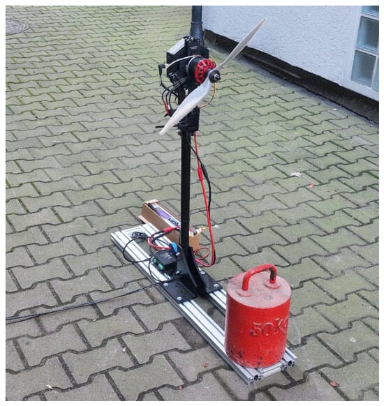
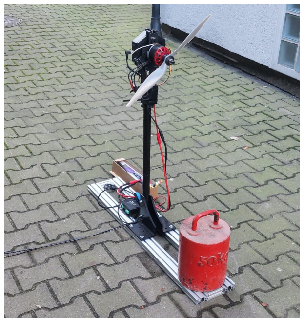
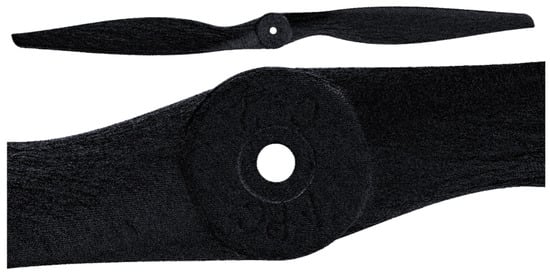
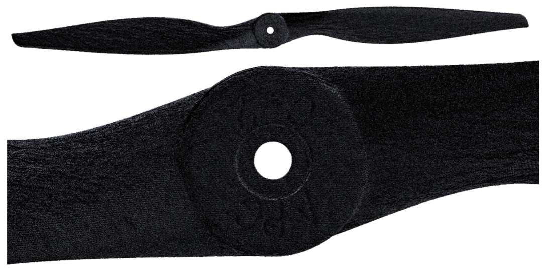
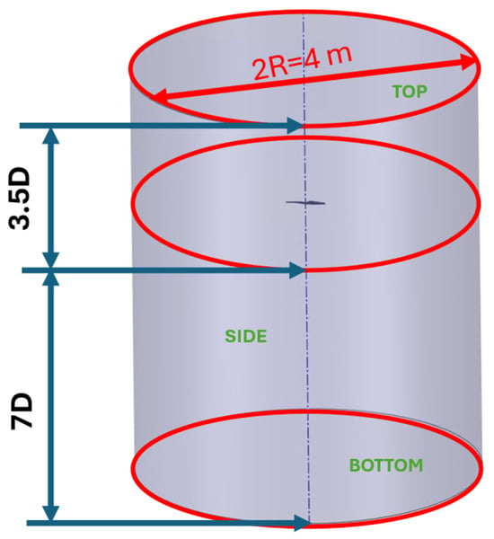
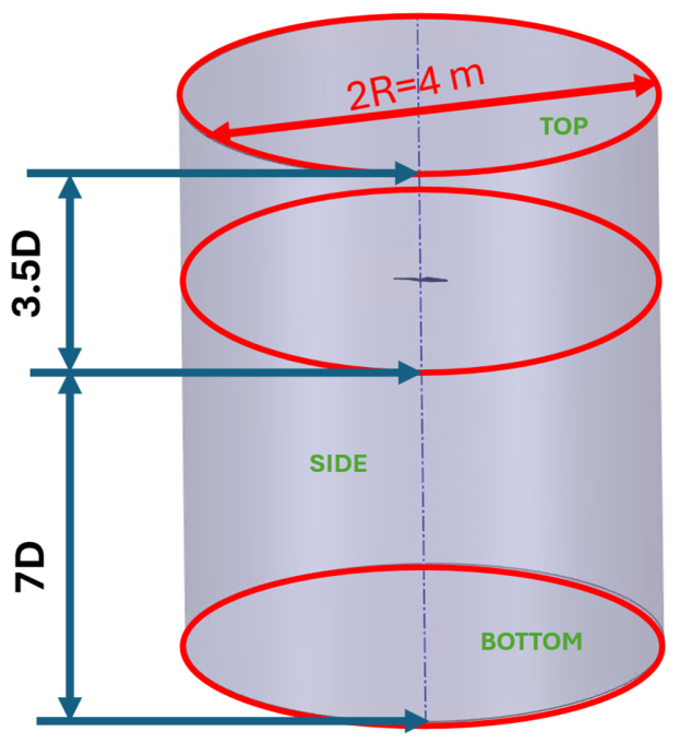
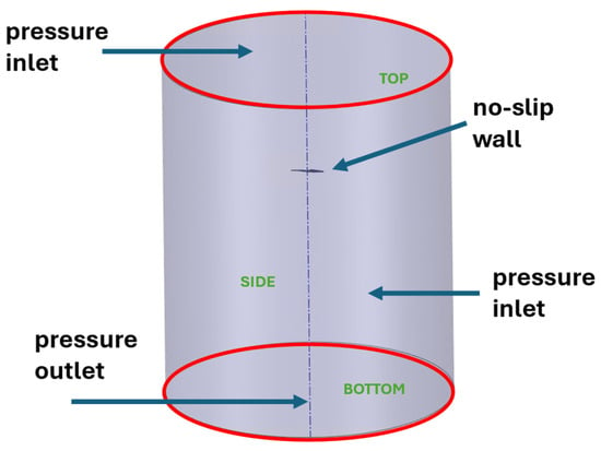
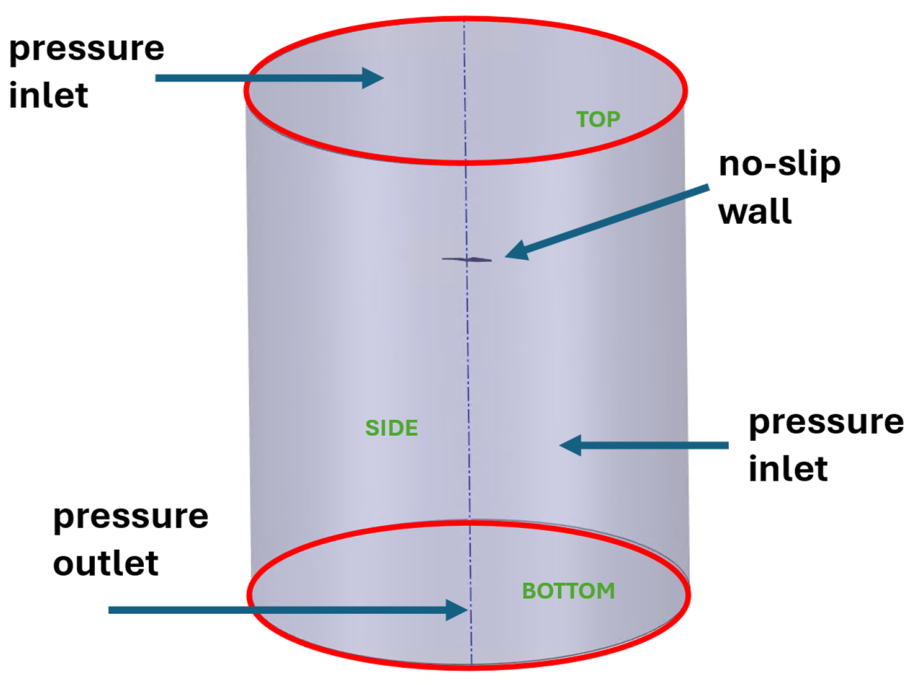
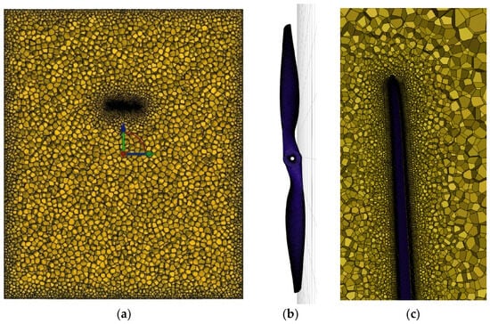
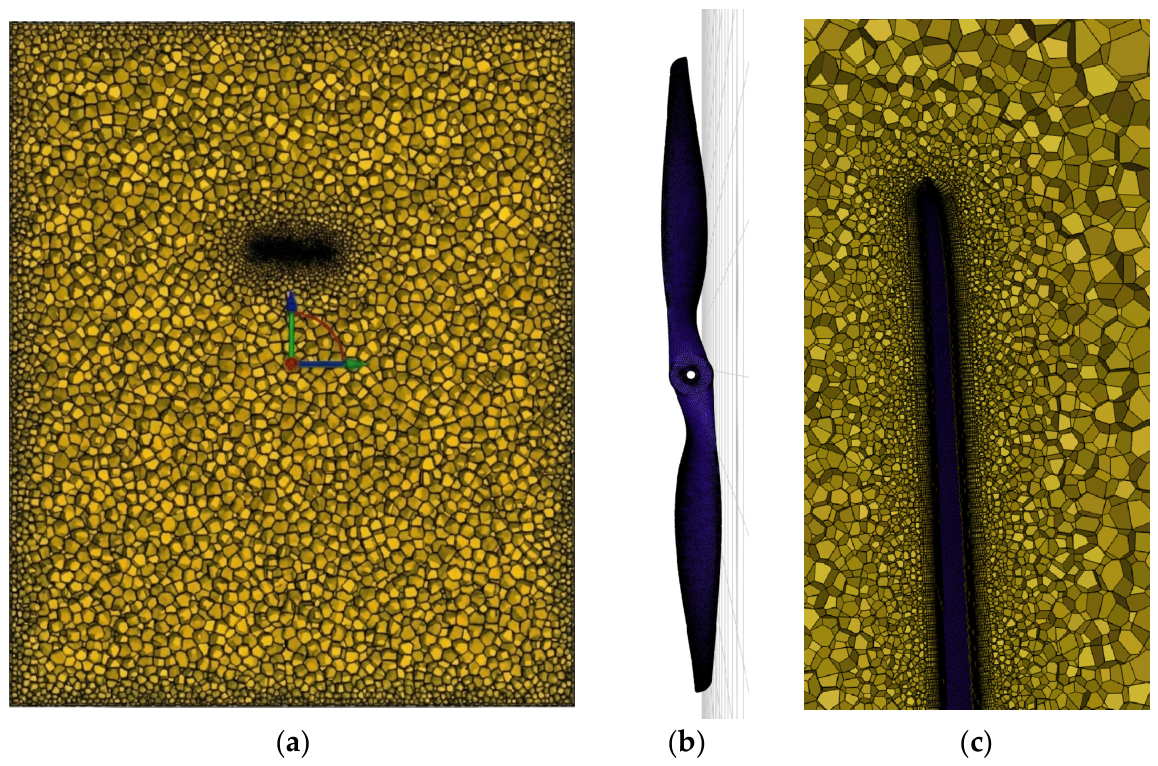
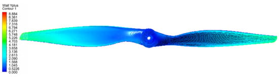
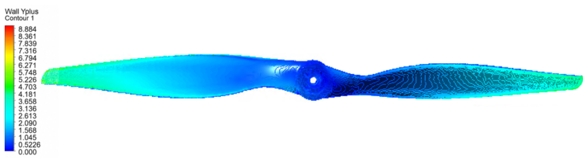
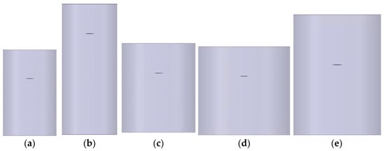
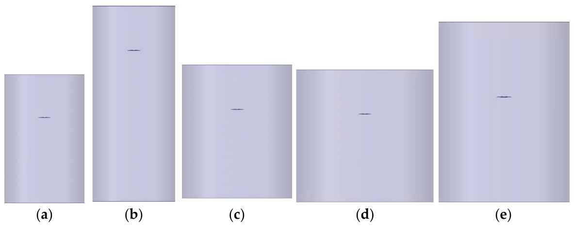
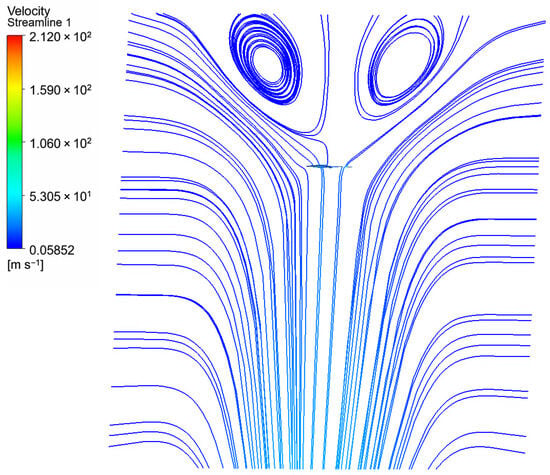
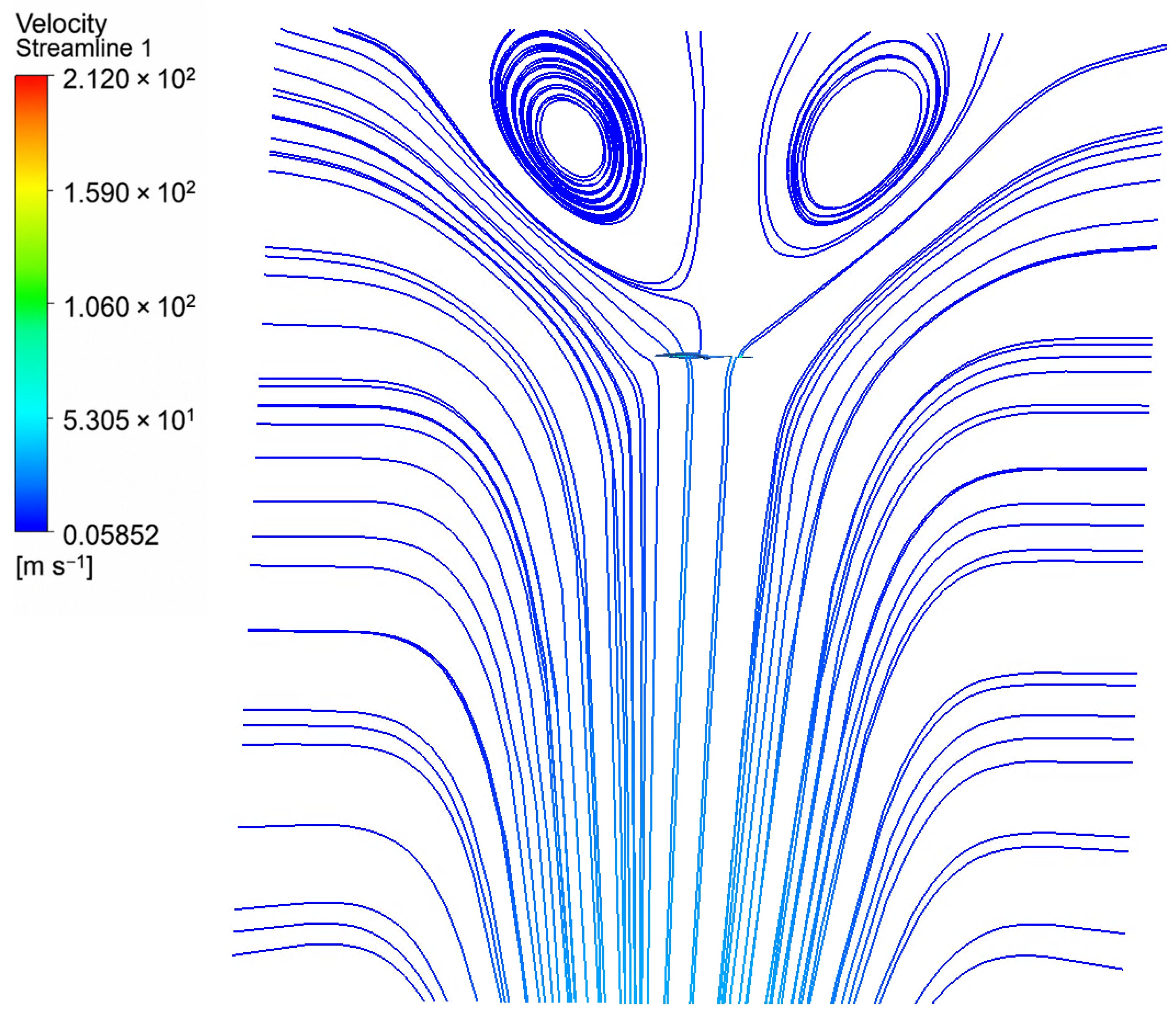
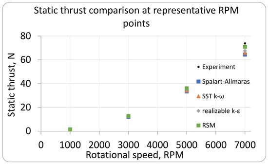
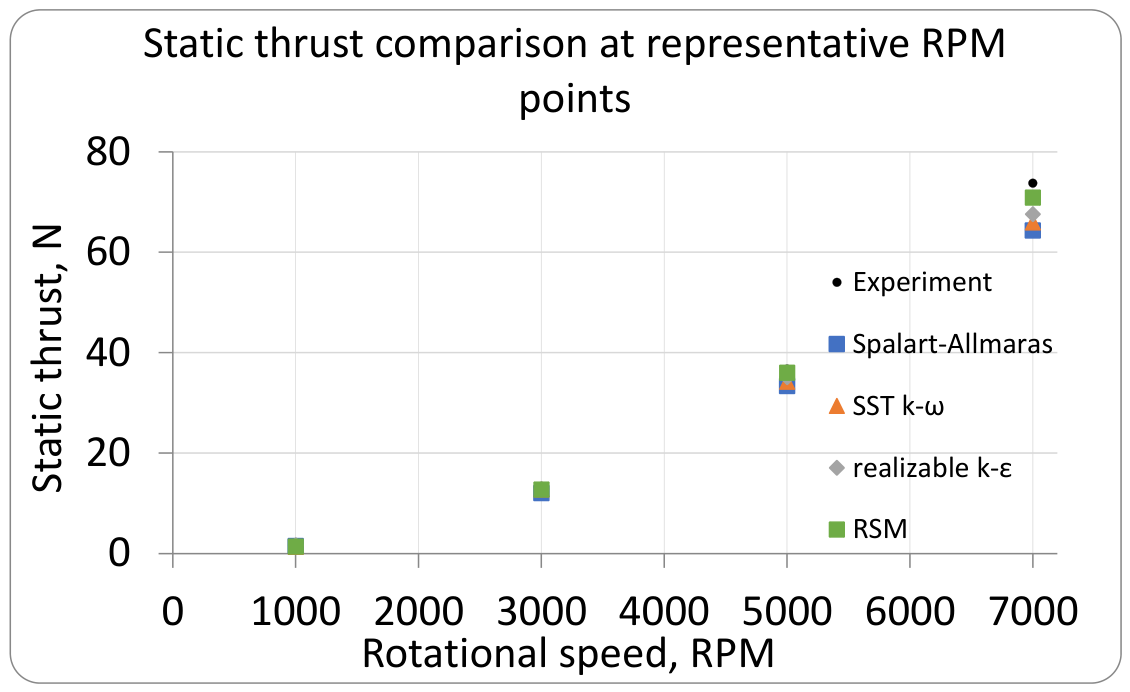
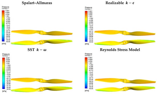
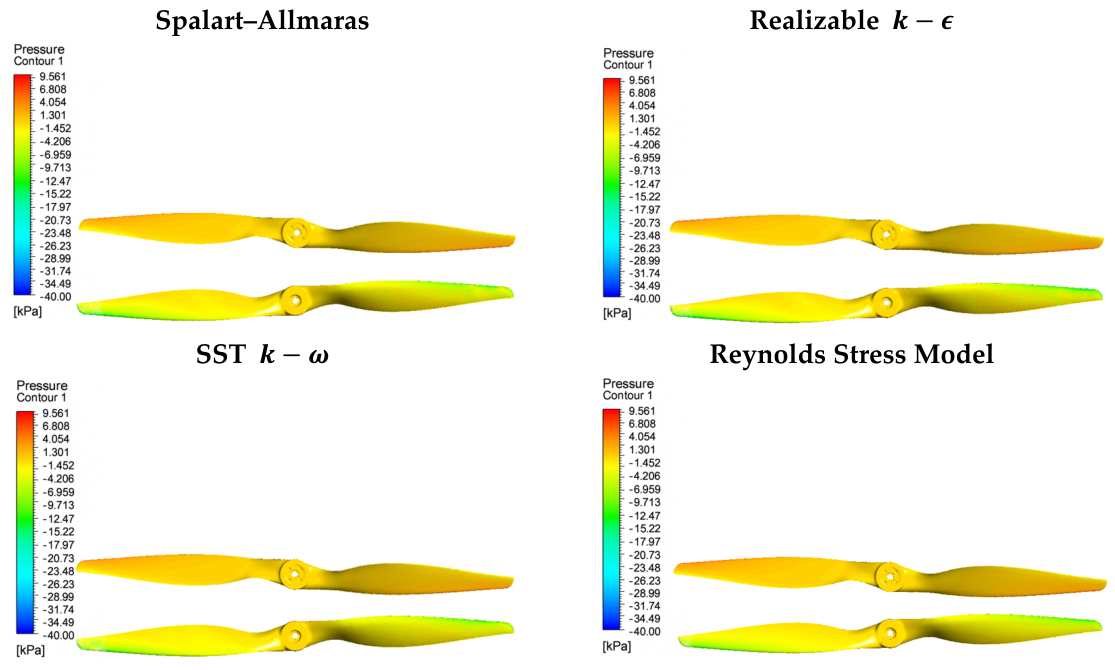
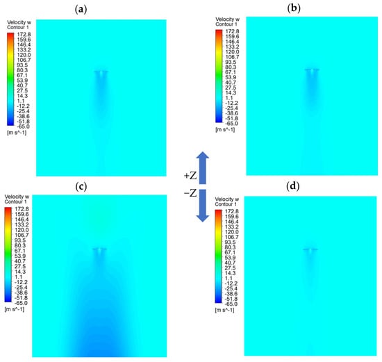
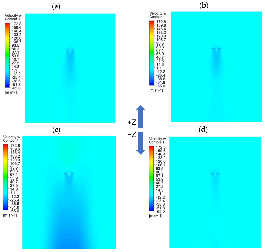

Disclaimer/Publisher’s Note: The statements, opinions and data contained in all publications are solely those of the individual author(s) and contributor(s) and not of MDPI and/or the editor(s). MDPI and/or the editor(s) disclaim responsibility for any injury to people or property resulting from any ideas, methods, instructions or products referred to in the content. |
© 2026 by the authors. Licensee MDPI, Basel, Switzerland. This article is an open access article distributed under the terms and conditions of the Creative Commons Attribution (CC BY) license.