


Abstract
This study presents a methodology for cross-ranking analysis to evaluate the consistency of universities’ positions across the QS World University Rankings, Times Higher Education (THE) World University Rankings, and Academic Ranking of World Universities (ARWU). Data for 2022–2025 were harmonized by university names, countries, years, and ranking positions, resulting in a unified dataset of 316 observations. Ranking agreement was assessed using the overlap of ranked lists, a Spearman distance–based similarity measure, and a normalized inverse-rank metric. QS rankings were treated as the response variable, while THE and ARWU positions served as predictors. Model performance was evaluated using leave-one-year-out cross-validation for a median baseline, the average of THE and ARWU ranks, linear regression, Random Forest, and XGBoost. Random Forest achieved the lowest mean absolute error (MAE = 24.80 ± 3.26 ranking positions), whereas linear regression best preserved relative ordering (Spearman’s ρ = 0.794 ± 0.062). Additional analyses of the TOP-50, TOP-100, and TOP-200 subsets showed that prediction accuracy decreases as ranking depth increases. The findings demonstrate that QS, THE, and ARWU provide complementary rather than interchangeable assessments of university performance. The proposed framework is intended for comparative cross-ranking analysis rather than forecasting future university rankings.
1. Introduction
Global university rankings have become one of the most influential instruments for evaluating higher education institutions. They are used not only by prospective students and parents, but also by university administrators, governmental agencies, international partners, and funding organizations. Although rankings cannot fully reflect the overall quality of a university, they significantly influence institutional reputation, international collaboration, student recruitment, and strategic planning. Consequently, understanding the mechanisms underlying the formation of ranking positions has become not only a scientific challenge but also an important practical task [1,2,3].
At the same time, university rankings cannot be considered neutral or uniform measurement systems. QS, Times Higher Education (THE), ARWU, and other ranking frameworks rely on different indicators, weighting schemes, data sources, and methodological assumptions. Some rankings place greater emphasis on reputation and international activity, whereas others focus more strongly on research productivity, citation impact, or academic achievements [4,5,6,7]. Consequently, the same university may occupy substantially different positions across ranking systems. This creates a significant challenge for universities, as ranking outcomes are actively used in managerial decision-making, while their interpretation is not always straightforward.
Previous studies have examined university rankings from multiple perspectives. A number of studies focus on the influence of rankings on educational policy and institutional behavior [1,2,3,4]. Other works compare ranking methodologies and demonstrate that differences in indicators, data coverage, and calculation principles may lead to substantial variations in final ranking positions [5,6,7]. A separate research direction is associated with bibliometric indicators, citation impact, and research performance, since these parameters constitute the foundation of many ranking systems [8,9,10,11]. In recent years, machine-learning and data-driven methods have also been applied to educational analytics and university ranking problems [12,13,14,15,16,17].
Despite the significant number of studies devoted to global university rankings, the quantitative relationship between the rankings of the same university across different ranking systems has not yet been sufficiently explored. Most studies compare the methodologies of QS, THE, and ARWU or examine the application of machine learning to specific indicators of university performance. At the same time, the task of cross-ranking assessment—where a university’s position in one system is determined based on its positions in other systems—is encountered significantly less frequently.
This paper proposes a unified analytical approach that combines the comparison of ranked lists with regression modeling. In the first stage, the similarity between the QS, THE, and ARWU rankings is assessed, taking into account the composition of the universities and differences in their positions. To do this, we use the overlap between the lists, Spearman’s distance, and the inverse rank metric. In the second stage, a university’s position in the QS rankings is treated as the target variable, while its positions in THE and ARWU are used as input features.
It is important to note that this approach does not constitute a prediction of the university’s future ranking. The data from QS, THE, and ARWU correspond to comparable ranking years, so this is an inter-ranking assessment and analysis of the relationships between different ranking systems. This approach allows us to determine the extent to which positions in THE and ARWU may be related to the position in QS, but it does not imply that one ranking system can completely replace another.
This study addresses two interrelated questions. First, to what extent do the QS, THE, and ARWU rankings agree in terms of the composition and relative order of universities at different Top-k levels? Second, how accurately can a university’s position in the QS rankings be estimated based on its positions in the THE and ARWU rankings for the same ranking year? To answer the first question, we used pairwise similarity metrics OS, F, and M. The second question was addressed as an inter-ranking regression problem using observations for which rankings in all three rankings are available simultaneously. Predicting publication citations was not included in the scope of this study.
The main contributions of this study are as follows:
- A consistent, multi-year dataset was compiled, combining university rankings from QS, THE, and ARWU for 2022–2025;
- A comparison of universities was conducted, taking into account variations in name spelling, country of origin, identical ranks, and rank intervals;
- A unified framework for the problem of cross-ranking QS positions based on THE and ARWU rankings has been proposed;
- An experimental design has been developed to compare simple baseline approaches, linear regression, Random Forest, and XGBoost;
- The robustness of the results was tested for the TOP-50, TOP-100, and TOP-200 samples, as well as across different ranking years;
- The limitations of the obtained estimates are discussed, taking into account differences in the methodologies, indicators, and calculation principles of QS, THE, and ARWU.
The rest of the article is organized as follows. Section 2 reviews previous studies on university rankings, the comparison of ranked lists, and the application of machine learning in educational analytics. Section 3 describes the data sources, the procedure for harmonizing them, similarity metrics, and the formulation of the inter-ranking regression problem. Section 4 presents the results of model comparisons, error analysis, and sensitivity tests for the TOP-50, TOP-100, and TOP-200 samples. Section 5 discusses the results obtained and the main limitations of the study. Section 6 presents the conclusions and directions for further work.
2. Related Work
Global university rankings are widely discussed in higher education research, as they influence not only the external reputation of universities but also student choice, international collaboration, and strategic planning. The works of Ellen Hazelkorn [1], David Dill and Maarja Soo [2], and Simon Marginson [3] show that rankings are more than just reference tables. Over time, they begin to influence the behavior of the universities themselves. At the same time, the authors note that ranking results should be interpreted with caution, since the complex activities of a university are reduced in these rankings to a limited set of indicators.
The second group of studies focuses on the methodological structure of global rankings. QS, THE, and ARWU use different sets of indicators, weighting coefficients, data sources, and methods for presenting final rankings [4,5,6,7,18,19,20]. These differences explain why the same university may occupy different positions in different ranking systems. These differences explain why the same university may rank differently in various ranking systems. Therefore, a simple visual comparison of the lists is not sufficient. Additional metrics are needed that take into account not only the presence of the same universities but also the differences in their rankings [21,22,23,24].
Comparative studies show that a university’s final ranking depends on the methodological assumptions underlying the ranking, the set of indicators, and the weighting scheme used [5,6,7]. Therefore, the similarity of rankings cannot be assessed solely based on the overlap in the universities listed; their relative positions within the lists must also be taken into account [22,25]. This provides the basis for using the intersection of sets, Spearman’s distance, and the inverse rank metric in this study.
A separate area of research focuses on bibliometric indicators. In the works of Ludo Waltman [8], Henk F. Moed [9], Lutz Bornmann and Loet Leydesdorff [10], as well as Cassidy R. Sugimoto and Vincent Larivière [11], it has been shown that publication activity and citation rates can be used to assess scientific performance, but they do not provide a complete and unambiguous picture of it. These metrics are influenced by the scientific field, the scope of the database, the age of the publication, and citation practices specific to a given discipline. This is particularly important for the present study because bibliometric indicators are incorporated into the methodology of global rankings. However, the number of citations for individual publications is not considered an independent dependent variable in this study.
In recent years, machine learning (ML) methods have been increasingly used to analyze higher education data. In recent years, machine learning methods have been increasingly used to analyze higher education data and university rankings [12,17]. Linear models are typically used as a simple and straightforward baseline. Random Forest allows for nonlinear relationships and interactions between features [13], while gradient boosting methods, including XGBoost, iteratively refine the model by adding new trees [14,16]. However, a more complex algorithm does not necessarily yield a more accurate or robust result; therefore, it must be compared with simple baseline approaches using identical data splits.
This is particularly relevant when analyzing university rankings, as rankings are determined based on different metrics, weightings, and methodological principles. At the same time, using a complex ML model does not in itself guarantee a more reliable result. Therefore, its quality must be compared with simple, basic approaches using identical data samples.
This review shows that research on global university rankings is developing primarily in two directions. The first involves comparing methodologies, indicators, and the final rankings of universities in the QS, THE, ARWU, and other ranking systems. The second direction examines the application of statistical methods and machine learning to higher education data.
However, these approaches are not always combined within a single experiment. Studies comparing rankings are often limited to describing methodological differences, while research using machine learning frequently focuses solely on the values of quality metrics. At the same time, differences in the principles underlying the construction of the rankings themselves are not always taken into account.
The work by Udupi et al. [12] is similar to the present study in terms of the general problem formulation, as it examines the application of machine learning and regression methods to evaluate global university rankings. In the present work, this approach is expanded by combining several analytical procedures within a single experiment. In addition to the regression-based estimation of QS rankings based on THE and ARWU rankings, a pairwise similarity analysis of the ranked lists from QS, THE, and ARWU is conducted using a consistent multi-year dataset covering 2022–2025. The study by Udupi et al. is indeed devoted to the application of regression models to the task of evaluating university rankings.
The robustness of the results in this study was assessed using the “leave-one-year-out” method, in which one ranking year was used for testing and the remaining years for training. The trained models were compared not only with each other but also with simple baseline approaches. Additionally, the sensitivity of the results was tested for the TOP-50, TOP-100, and TOP-200 samples. Thus, this study does not claim to offer a completely novel approach to the task of evaluating university rankings, but rather expands upon existing research by combining data harmonization, analysis of the similarity of ranked lists, inter-ranking regression, and inter-year validation.
3. Materials and Methods
Global university ranking data has a heterogeneous structure. QS, Times Higher Education, and ARWU use different methodologies, sets of indicators, and methods for presenting final rankings. In addition, ranking tables may contain identical ranks, range-based positions, and different spellings of the same university’s name. Therefore, directly combining such data without prior coordination can lead to errors and incorrect comparisons between institutions [18,19,20,21].
This study employs a sequential data preparation procedure. First, the ranking tables for the relevant years are standardized to a common structure. Next, the names of universities and countries are standardized, duplicates are removed, and rank values are converted to a comparable numerical format. For ARWU, range-based rankings are processed separately, since some universities are represented not by an exact rank but by a range, such as 101–150. Afterward, a sample of observations is formed for which QS, THE, and ARWU rankings are all available for the same ranking year.
The machine learning problem is formulated as a regression problem. A university’s numerical ranking in QS is used as the target variable, while its corresponding rankings in THE and ARWU are used as input features. This formulation allows us to assess the extent to which a university’s position in two ranking systems is related to its position in the third. However, the model is not intended as a tool for accurately predicting a university’s future ranking, since the input and target rankings refer to the same ranking cycle. This study focuses specifically on cross-ranking assessment.
3.1. Methodological Workflow
The overall research workflow is shown in Figure 1. It includes collecting ranking data from QS, THE, and ARWU; harmonizing university names and ranking years; processing related positions and rank intervals; forming a combined sample; calculating similarity metrics; training regression models; and analyzing errors.
Figure 1.
Methodological workflow of the cross-ranking analysis: data collection, harmonization, similarity assessment, regression modeling, validation, and interpretation of results. The numbered boxes represent the sequential stages of the proposed workflow, the arrows indicate the direction of data processing, and the colors are used solely to visually distinguish the workflow stages.
Similarity analysis and regression modeling were performed using a single, harmonized dataset, but addressed different aspects of the overall research question. In the first stage, the extent to which the rankings coincided in terms of the composition of universities and their relative order was determined. In the second stage, the numerical QS ranking was evaluated against the corresponding THE and ARWU rankings.
The OS, F, and M values were not used as input variables for the regression models. Their role was to provide a preliminary characterization of inter-ranking consistency and to facilitate the subsequent interpretation of model errors. To analyze similarity, independent pairwise Top-k lists were formed, whereas the regression analysis was conducted only on the triple intersection of QS, THE, and ARWU. Thus, the two stages are linked by a common data harmonization procedure and a common research objective, but they use different analytical subsets.
3.2. Data Integration and Analytical Pipeline
Data processing was carried out in stages. In the first stage, QS, THE, and ARWU ranking data for specific years were collected. Each source had its own structure, so the tables were standardized to a common format before being combined. During this same stage, column names, data types, and the presence of key ranking indicators were verified.
Next, data cleaning was performed. Duplicate records were removed, university and country names were standardized, and ranking positions were converted to numerical format. Special attention was paid to variations in the spelling of the names of the same university. Abbreviated and full versions were merged only when a match could be established unambiguously. Unrestricted automatic matching based on approximate similarity of names was not used [21].
After cleaning, the data were aggregated by university, country, and ranking year. Both complete and incomplete records were retained in the overall dataset. However, the main experiment included only observations for which QS, THE, and ARWU rankings were all available. This approach reduces the size of the final sample but avoids replacing missing rankings with artificially calculated or average values.
Special processing was applied to ARWU ranking intervals. If a university was represented by a range, such as 101–150, the lower and upper bounds of the range were retained in the original dataset. For the regression analysis, the midpoint of the range was used. This simplifies numerical modeling but does not obscure the fact that the original ranking was an interval rather than an exact value.
In the next step, similarity metrics for the ranked lists were calculated, and a sample was formed for regression analysis. Pairwise similarity between QS, THE, and ARWU was assessed separately for each ranking year and each TOP-k depth. Position metrics were calculated for universities included in the intersection of the corresponding pair of lists. For the regression analysis, the QS ranking was used as the target variable, while the THE and ARWU rankings were used as the two input features. We compared the median baseline model, the average of the THE and ARWU rankings, linear regression, Random Forest, and XGBoost. All approaches were evaluated on identical “leave-one-year-out” validation sets.
Additionally, the sensitivity of the results was tested for three sample sets: TOP-50, TOP-100, and TOP-200. This allowed us to assess how absolute errors change as the range of considered ranking positions expands.
The proposed framework is a sequential analytical process for preparing and analyzing rating data. This paper does not conduct a separate experimental study of computational scalability, distributed data storage, or the performance of Big Data infrastructure. Therefore, the conclusions of the study pertain to the quality of data harmonization, cross-rating comparisons, and the performance of regression models, rather than to the performance of the software platform.
3.3. Ranking Similarity Metrics and Parameter Definitions
To compare different global university rankings, this study employs similarity metrics that enable a more objective assessment of the degree of consistency between ranked lists. This is important because QS, THE, ARWU, and other ranking systems are based on different indicators, weighting schemes, data sources, and methodological assumptions. Consequently, the same institution may occupy different positions across rankings, even when broadly similar aspects of university performance are being evaluated.
The study uses three metrics: overlap size (OS), a similarity measure based on Spearman’s distance (F), and a normalized inverse rank metric (M). These metrics characterize different aspects of similarity: OS reflects the commonality of the lists’ composition, F accounts for differences in the order of shared universities, and M places greater weight on discrepancies at the top of the rankings. Overlap Size (OS) was used as a simple measure of the common composition of the two lists. The F measure is based on Spearman’s distance, which is defined as the sum of the absolute differences between the ranks of common elements [22]. The normalized metric M was applied as an additional indicator, more sensitive to discrepancies at the top of the ranking list; its calculation is provided below. These metrics characterize different aspects of similarity: OS reflects the commonality of the lists’ composition, F accounts for differences in the order of shared universities, and M places greater weight on discrepancies at the top of the ranking [26].
The OS overlap was used as a simple measure of the overall composition of the two lists. The F-measure is based on Spearman’s distance, which is defined as the sum of the absolute differences between the ranks of the common elements [27]. The normalized metric M was used as an additional indicator, one that is more sensitive to differences at the top of the ranking list; its calculation is provided below.
3.3.1. Definitions of Symbols and Parameters
In the formulas below, A and B denote the two ranking lists being compared, and denotes a specific university. The set consists of universities that appear in both rankings. The value indicates the number of such universities.
The functions and denote the position of university i in rankings A and B, respectively. The lower the rank value, the higher the university’s position. The parameter k specifies the depth of the list being compared, such as TOP-50, TOP-100, or TOP-200.
For universities tied for the same position, the average rank is used. If several universities are tied for a single position, each is assigned the same average value calculated for the corresponding range of ranks. This approach avoids artificially establishing an order among the universities [28].
This paper uses three main metrics. The symbol OS denotes the size of the intersection of the ranking lists, F denotes a normalized similarity measure based on Spearman’s distance, and M denotes a normalized inverse-rank metric. The M metric places greater weight on discrepancies occurring at the top of the ranking list.
If ARWU publishes a rank range rather than an exact rank, the midpoint of that range is used in the regression analysis:
where and denote the lower and upper bounds of the published rank range, respectively. Both bounds are retained in the original dataset.
Similarity metrics are not used to construct a new composite ranking and do not replace the original QS, THE, or ARWU rankings. They are used to assess the degree of consistency among ranking systems and to interpret the results of the regression analysis.
3.3.2. Similarity Metrics for Ranked Lists
Overlap Size, OS. The Overlap Size metric represents the number of common elements shared by two ranking lists. In the context of this study, these elements correspond to universities simultaneously present in both compared rankings. Formally, the metric can be expressed as follows:
where and denote two ranking lists being compared, and represents the number of universities included in both lists.
Despite its simplicity, this metric is useful at the initial stage of analysis because it allows the degree of overlap between rankings in terms of university composition to be assessed. However, has an important limitation: it does not account for the ordering of universities within the ranking lists. For example, two rankings may contain the same universities while arranging them in entirely different sequences. Therefore, in the present study, is not used independently, but rather in combination with position-sensitive similarity metrics.
Spearman’s Footrule, F. The Spearman distance-based similarity measure takes into account not only the presence of the same universities in both rankings, but also the differences in their positions. First, the set of universities that appear in both lists being compared is identified:
Before calculating the distance, the universities in set C are re-ranked within the overall set from 1 to n. The resulting ranks are denoted as and . If several universities have the same rank, their average rank is used.
The Spearman absolute distance and its maximum possible value are defined as follows:
here, denotes rounding down to the nearest integer. The normalized distance is calculated as:
The final similarity measure is defined as follows:
The value of ranges from 0 to 1. The closer it is to 1, the smaller the difference in the rankings of the universities in question. A value close to 0 indicates a significant discrepancy between their rankings.
Inverse Rank, . The inverse-rank metric is used to give greater weight to differences at the top of the ranking list. After re-ranking the universities within the overall set C, the unnormalized value is calculated as follows:
If a university’s ranking is the same on both lists, the denominator of the corresponding term is equal to one. As the difference between the rankings increases, that university’s contribution decreases [29].
For a fixed number of general universities, , the maximum possible value of IR is determined across all possible pairs of rankings of these n universities after they have been reordered within the set . The maximum is reached when the positions coincide exactly, that is, when each rank in list corresponds to the same rank in list :
Thus, is an analytically defined normalizing value for a fixed intersection size n. It is not defined as the largest value among the observed pairs of ratings and does not depend on whether a rating is compared with itself.
The normalized inverse rank metric is calculated using the following formula:
The value of ranges from 0 to 1. The closer it is to 1, the higher the agreement between the two rankings, particularly at the top of the compared lists. Compared to the intersection size and the -measure, the metric is more sensitive to changes in the order of the top universities. The positional metrics and were calculated only for universities that are part of the intersection of the two TOP-k lists, that is, for the set C = A ∩ B. Before calculating the metrics, these universities were re-ranked within the overall set. Institutions appearing in only one of the two lists were not included in the calculation of the positional distance.
Universities that were not included were accounted for via the OS metric, but they were not assigned a separate penalty position when calculating F and M. Therefore, when there is little overlap between the lists, the positional similarity values may slightly overestimate the overall degree of agreement: the metrics evaluate the order only among the universities common to both lists and do not penalize differences in the composition of the lists. For this reason, OS, F, and M were interpreted collectively, rather than as interchangeable metrics. A brief numerical example.
Consider two hypothetical TOP-4 lists:
The universities , and are common to both lists. Therefore,
After re-ranking the universities within the set C, their positions are as follows (Table 1):
Table 1.
Method of determining positions after revising the ranking of universities in the C set.
Spearman’s absolute distance is:
For three general universities, the maximum possible distance is equal to:
In that case, the normalized similarity measure is:
The unnormalized value of the inverse rank metric is calculated as:
The maximum possible value of the metric is
Therefore,
University appears only in List A, while University appears only in List B. They reduce the size of the intersection between the lists but do not incur a separate positional penalty when calculating F and M. This example illustrates why positional metrics must be considered in conjunction with the OS metric.
3.3.3. Handling of Tied Positions
Rankings may include tied positions, where multiple universities share the same rank. In such cases, each university is assigned the average rank of the corresponding range:
here, denotes the first position in a group of tied ranks, denotes the last position, and m denotes the number of universities tied for that rank. This approach avoids the need to artificially establish an internal order among the universities.
3.3.4. The Purpose of Cross-Rating Assessment
After comparing the rankings, the machine learning problem is formulated as a regression problem. For each university i and ranking year t, we need to estimate its QS ranking based on its corresponding rankings in THE and ARWU:
here, denotes the actual ranking of university i in the QS rankings for ranking year t, and denotes the ranking estimated by the model. The variables and correspond to the rankings of the same university in the THE and ARWU rankings for the comparable ranking year.
For ARWU’s interval rankings, the midpoint of the published rank range is used. The function describes the inter-ranking relationship; denotes the relationship obtained after training the model; and represents the residual error.
Since the target QS ranking and the input THE and ARWU rankings all pertain to the same ranking year, this problem is treated as an inter-ranking estimation. It does not predict a future value and does not determine what position a university will occupy in the next ranking issue.
3.4. Data Collection and Preprocessing
This study utilized data from three global university rankings: the QS World University Rankings, the Times Higher Education World University Rankings, and the Academic Ranking of World Universities. To form the overall sample, ranking data for 2022–2025 were collected. This study was entirely computational and was based exclusively on digital university-ranking datasets. No chemicals, reagents, biological samples, commercial cell lines, laboratory materials, physical devices, or scientific instruments were used in this study.
The working technical file was generated based on the World University Rankings 2026 Dataset [23]. The 2022–2025 editions were used for the main analysis. Information on the ranking editions, publication dates, and source structure was additionally cross-checked against the official websites of QS, THE, and ARWU [18,19,20].
The observation unit was the “university–ranking year” pair. For each observation, the university name, country, ranking year, and rankings in QS, THE, and ARWU were recorded. The country name and year were used to further verify the consistency of records when merging data sources. Only the THE and ARWU rankings were used as input variables for the regression model, while the QS ranking served as the target variable.
Preprocessing was performed separately for each source. Column names and data types were standardized to a common structure, and duplicate records and technical characters were removed. University names were standardized, taking into account both full and abbreviated spellings. Records were merged only in cases where the university could be unambiguously identified. The country and ranking year were additionally verified, which helped reduce the risk of erroneous matching of institutions with similar names [21].
Ranking positions were converted to numerical values. For tied positions, information on the associated rank was retained. If ARWU published a rank range rather than an exact position—for example, 101–150 the lower and upper bounds of that range were retained in the original dataset. For regression analysis, the midpoint of the published range was used.
After standardization, the QS, THE, and ARWU data were merged by university name, country, and ranking year. The main experimental sample included only those observations for which positions in all three rankings were available simultaneously. Missing rankings were not replaced with averages, medians, or other artificially calculated values.
Data sources, ranking editions, and the main stages of forming the analytical sample are presented in Table 2. The unit of analysis at all stages was a “university–ranking year” record. Before consolidation, the names of universities and countries, ranking years, numerical rankings, duplicates, and technical designations were verified separately for each ranking.
Table 2.
Data sources, rating reports, and the process of forming the analytical sample.
The complete technical file contained QS and THE data for 2022–2026 and ARWU data for 2022–2025. Since there was no comparable ARWU data for 2026, the main analysis was limited to the period 2022–2025. After this restriction, the combined table contained 1206 entries: QS rankings were available for 803 observations, THE rankings for 637, and ARWU rankings for 770. Rankings in all three rankings were identified for 316 observations.
After selecting records with simultaneously available QS, THE, and ARWU rankings, a complete analytical sample of 316 observations for 2022–2025 was formed. Each observation corresponds to one university in a single ranking year. The distribution of this sample by year is presented in Table 3.
Table 3.
Distribution of Complete QS–THE–ARWU Observations by Ranking Year.
As shown in Table 3, the number of complete observations varies by year. This is due to the varying coverage of universities in the source ranking tables, as well as the requirement that a university be ranked simultaneously in the QS, THE, and ARWU rankings. Consequently, the final dataset is unbalanced across years, a factor that is taken into account in the subsequent evaluation of the models.
For the sensitivity analysis, additional TOP-50, TOP-100, and TOP-200 samples were formed. The study employed two different principles for forming TOP-k samples. To analyze similarity for each pair of rankings and each year, two TOP-k lists were formed independently. For example, when comparing QS and THE, universities ranked in both systems were considered; an ARWU ranking was not required for such a comparison. The size of the pairwise intersection was used to calculate OS, F, and M.
A stricter criterion was applied for the regression analysis. It included only those observations for which QS, THE, and ARWU rankings were all available simultaneously. When forming the TOP-50, TOP-100, and TOP-200 regression samples, a university had to fall within the corresponding threshold in all three rankings at the same time. Therefore, the sizes of the regression samples do not match the pairwise intersection sizes used in the similarity analysis. For the sensitivity analysis, TOP-50, TOP-100, and TOP-200 subsamples were formed from the complete triple sample. An observation was included in the corresponding subsample only if the university’s ranking simultaneously fell within the specified thresholds in the QS, THE, and ARWU rankings. As a result, the TOP-50, TOP-100, and TOP-200 subsamples contained 60, 135, and 316 observations, respectively.
3.5. Model Configuration and Validation Procedure
To evaluate a university’s position across different rankings, five approaches were compared in the QS analysis: the median baseline model, the average of THE and ARWU rankings, linear regression, Random Forest (RF), and XGBoost. In all cases, the QS ranking was used as the target variable, while the THE and ARWU rankings served as the two input features.
The median baseline model assigned the median QS ranking—calculated solely from the training sample—to all observations in the test year. The second baseline model estimated the QS score as the arithmetic mean of the THE and ARWU rankings. These simple variants were used to verify whether the trained models provided a noticeable improvement over elementary rules. Linear regression was applied without additional regularization or separate hyperparameter tuning.
An 80/20 random split of the data was not used. The main evaluation procedure was year-over-year validation using the “leave-one-year-out” method. At each step, all observations from a single rating year formed the external test set, while data from the remaining three years were used to train the model. The procedure was repeated sequentially for the years 2022, 2023, 2024, and 2025.
As a result, four external splits were formed. When testing on the 2022 data, the training sample contained 212 observations, and the test sample contained 104. For 2023, 240 training and 76 test observations were used. The same ratio was applied when testing on the 2024 data. In the final step, the models were trained on 256 observations from 2022–2024 and evaluated on 60 observations from 2025.
The RF and XGBoost hyperparameters were tuned separately within each external training set. For internal validation, GroupKFold cross-validation (CV) was used, with observations grouped by rating year. Since the training set of each external split contained data from three rating years, the internal CV procedure included three group splits. Observations from the external test year were not used for either parameter selection or model training. Observations from the external test year were not used for either parameter selection or model training.
Parameter tuning was performed using GridSearchCV. The selection criterion was the mean absolute error. In the scikit-learn implementation, the ‘neg_mean_absolute_error’ metric was used; therefore, the combination of parameters with the lowest actual MAE value was considered the best. After internal validation, the model with the selected parameters was retrained on the entire external training set and then applied to the observations from the reserved test year [30].
The following hyperparameter values were tested for RF:
- Number of trees n_estimators: 300 and 500;
- Maximum tree depth max_depth: no limit, 6, and 12;
- Minimum number of samples in a leaf node min_samples_leaf: 1, 2, and 3;
- Number of features considered at each split, max_features: 1, 0, and “sqrt”.
Since the model used only two input features, the option max_features = “sqrt” effectively meant that a single randomly selected feature was considered when forming each tree split.
The following values were tested for XGBoost:
- Number of trees n_estimators: 200 and 400;
- Maximum tree depth max_depth: 2 and 3;
- Learning rate learning_rate: 0.03 and 0.07;
- Minimum sum of observation weights in a child node min_child_weight: 1 and 5.
The subsample and colsample_bytree parameters were set to 0.9. The objective = “reg:squarederror” function was used to solve the regression problem, and the trees were constructed using the tree_method = “hist” parameter.
To ensure reproducibility, a fixed value of ‘random_state = 42’ was used in all stochastic procedures. Parallel processing was performed with the parameter ‘n_jobs = −1’. Hyperparameter tuning was performed anew in each out-of-fold split, so the selected combinations could vary between individual test years.
After generating the combined out-of-fold estimates, the validity of the calculated QS scores was additionally verified. Since the main regression experiment was conducted on the TOP-200 sample, the acceptable range was set from 1 to 200. The presence of zero and negative values, scores below 1, and values above 200 was checked separately.
The metrics were calculated based on the models’ original continuous estimates without rounding to integer positions. No forced value constraints, range clipping, or target variable transformations were applied. This approach made it possible to avoid artificially reducing errors through subsequent adjustment of the results. The actual values of the minimum and maximum estimated positions, as well as the results of the valid-range check, are presented in Section 4.4.
The split, in which the models were trained on data from 2022–2024 and evaluated on observations from 2025, is one of four external steps in the leave-one-year-out validation.
Its results are presented separately below for a more detailed examination of the models’ performance during the most recent ranking cycle, but are not considered an additional or independent validation. Note that the starting positions for THE and ARWU and the target position for QS all refer to the same ranking year. Therefore, this breakdown characterizes the transferability of inter-ranking relationships across ranking cycles, rather than the model’s ability to predict a university’s future ranking.
All computations were performed in the Google Colaboratory cloud environment (Google LLC, Mountain View, CA, USA) using Python 3.12.13 (Python Software Foundation, Beaverton, OR, USA). NumPy 2.0.2 (NumPy Developers, open-source software) and pandas 2.2.2 (pandas development team, open-source software) were used for data processing and transformation. Linear regression, Random Forest, GroupKFold cross-validation, GridSearchCV hyperparameter tuning, and performance-metric calculations were implemented using scikit-learn 1.6.1 (scikit-learn developers, open-source software). The gradient-boosting model was implemented using XGBoost 3.3.0 (XGBoost developers, open-source software). The experiments were executed using Linux kernel 6.6.122+ (Linux kernel developers, open-source software) on an x86_64 architecture with GNU C Library (glibc) 2.35 (GNU Project/Free Software Foundation, Boston, MA, USA). NumPy, pandas, scikit-learn, XGBoost, and Linux are community-developed open-source projects and do not have a single commercial manufacturer; therefore, a manufacturer’s city and country are not applicable to these software packages. The computational environment provided two logical CPU cores. All models were trained on the CPU without dedicated GPU acceleration or distributed computing infrastructure.
3.6. Evaluation Metrics
Model quality was evaluated using the mean absolute error (MAE), the root mean square error (RMSE), the median absolute error (MedAE), and the coefficient of determination R2. MAE indicates the average absolute magnitude of the discrepancy between the actual and estimated positions. RMSE is more sensitive to large errors, whereas MedAE is less sensitive to individual observations with large deviations.
Rankings are ordinal in nature. A lower numerical value corresponds to a higher university ranking; however, the same numerical distance does not necessarily have the same substantive meaning in different parts of the list. For example, a difference of ten positions among the leading universities and the same difference closer to the lower end of the TOP-200 are formally of equal magnitude but may be interpreted differently from a practical standpoint.
Ordinary regression was used in this study as a practical method to estimate the numerical magnitude of the discrepancy between the actual and calculated QS rankings. This use of regression does not imply that the ranking positions are treated as a full-fledged interval scale with equal distances between all adjacent positions [31].
For this reason, MAE, RMSE, MedAE, and R2 were not interpreted separately from the rank-based metrics. Additionally, Spearman’s ρ and Kendall’s τ correlation coefficients were calculated, which indicate the extent to which the model preserves the relative order of the universities. The combined use of these metrics allows for an assessment of both the numerical magnitude of the error and the quality of the reproduction of the sequence of universities in the ranking. For each method, the metrics were calculated separately for four external test years. The final results are presented as the mean and standard deviation across these four splits. This format shows not only the average level of quality but also its variability across individual ranking cycles.
4. Results
This section presents the results of a pairwise similarity analysis of QS, THE, and ARWU; a comparison of models for inter-ranking assessment of QS positions; a sensitivity analysis regarding list depth; and the distribution of out-of-fold errors in the Random Forest model. The main regression experiment was conducted on 316 observations from 2022–2025. Each observation corresponds to a “university–ranking year” pair and contains the simultaneously available QS, THE, and ARWU rankings. The target variable was the QS ranking, while the THE and ARWU rankings were used as input features.
4.1. Ranking Similarity Results
In the first stage, the similarity between the QS, THE, and ARWU rankings was assessed. Calculations were performed separately for each ranking year from 2022 to 2025, as well as separately for the TOP-50, TOP-100, and TOP-200. This approach ensures that the rankings of universities from different ranking cycles are not mixed.
For each pair of rankings, independent TOP-k lists were first generated. The overlap size indicated the number of universities appearing in both compared lists. A normalized measure based on Spearman’s F distance accounted for differences in the order of the universities overall. The inverse rank metric M, in turn, was more sensitive to discrepancies at the top of the list.
For each combination of rankings and list depth, four annual values were calculated. Table 4 presents their mean values and standard deviations for 2022–2025. This format shows not only the overall level of similarity but also its stability across individual ranking editions.
Table 4.
Pairwise Similarity Between the QS, THE, and ARWU Rankings: Means and Standard Deviations for the 2022–2025 Ranking Years.
As can be seen in Table 4, the results depend on the depth of the list under consideration and the selected metric. For the Top-50 sample, the highest average F-score was obtained for the THE–ARWU pair and amounts to 0.761. When moving to the TOP-200 sample, the highest value of this metric is observed for the QS–THE pair and amounts to 0.682. Therefore, it would not be entirely correct to identify a single most consistent pair of rankings for all list depths at once.
The largest average overlap size across all three samples was obtained for the QS–ARWU pair. For the TOP-200 sample, it amounts to 122.75 universities. However, the size of the overlap primarily characterizes the commonality of the lists’ composition and does not in itself imply that the universities’ rankings are close. This is evident from the M values: despite the relatively large overlap, the QS–ARWU pair shows lower consistency at the top of the list—ranging from 0.261 for the TOP-50 to 0.207 for the TOP-200.
The M values are generally lower than the F values. This result is to be expected, since the M metric takes greater account of the differences in the rankings of leading universities. In other words, two rankings may include a significant number of the same institutions but place them at the top of the list in markedly different orders.
Standard deviations also show that the similarity between the rankings varies from year to year. The annual variability in the overlap size is particularly noticeable for pairs that include THE. When interpreting these values, one should take into account not only actual changes in the rankings but also the varying coverage of the source tables. In the dataset used, the number of available THE and ARWU positions varies by year; therefore, the Overlap Size metric must be considered in conjunction with the results of the data completeness check.
Overall, the results show that QS, THE, and ARWU partially overlap in the composition of universities, but the closeness of their rankings depends on the pair being compared, the depth of the list, and the chosen metric. The obtained values do not allow these ranking systems to be considered interchangeable. The most noticeable differences remain at the top of the lists, reflected in comparatively lower values of the metric M. For a clearer presentation of the results, matrices of mean F and M values were constructed separately for the TOP-200 sample. Each cell shows the mean value of the corresponding metric for the ranking years 2022–2025. The TOP-200 sample was used for visualization as the broadest of the three samples considered. The results for the TOP-50 and TOP-100 are presented in full in Table 2 and are not duplicated in the figures.
Figure 2 shows the matrix of mean similarity measures based on Spearman’s F distance. The diagonal values equal one, as they correspond to a comparison of each ranking with itself. The off-diagonal displays the results of pairwise comparisons of QS, THE and ARWU.
Figure 2.
Matrix of mean similarity measures based on Spearman’s footrule (F) for independent pairwise TOP–200 lists of the QS, THE, and ARWU rankings. The cell colors correspond to the scale shown on the right: dark purple indicates lower similarity values, green and blue-green shades indicate intermediate values, and yellow indicates higher similarity values. The yellow diagonal cells with values of 1.000 represent comparisons of each ranking with itself.
Values were calculated separately for the 2022–2025 ranking years and then averaged across four annual comparisons. The position metric was calculated only for universities that are included in the intersection of the corresponding pair of lists. Diagonal values equal one and correspond to comparisons of each ranking with itself.
As Figure 2 shows, the highest average F value for the TOP-200 sample was obtained when comparing QS and THE and is 0.682. For the THE–ARWU pair, the value is 0.653, and for QS–ARWU, it is 0.618. Thus, at this depth in the list, the closest arrangement of common universities is observed between the QS and THE rankings. However, these values do not indicate complete alignment of the rankings: differences in the order of universities persist in all three pairs.
Figure 3 shows the matrix of mean values of the inverse rank metric M. Unlike the F measure, this metric places greater weight on discrepancies at the top of the ranking list. Therefore, it allows for a separate assessment of how closely leading universities are positioned in different ranking systems.
Figure 3.
Matrix of mean values of the normalized inverse-rank metric (M) for independent pairwise TOP–200 lists of the QS, THE, and ARWU rankings. The cell colors correspond to the scale shown on the right: dark purple indicates lower similarity values, blue and blue-green shades indicate intermediate values, and yellow indicates higher similarity values. The yellow diagonal cells with values of 1.000 represent comparisons of each ranking with itself.
Values were calculated separately for the 2022–2025 ranking years and then averaged across four annual comparisons. The metric was calculated only for universities that intersect the corresponding pair of lists and gave greater weight to discrepancies at the top of the ranking. Higher values correspond to greater consistency in the order of overall universities.
As Figure 3 shows, the M values are significantly lower than the corresponding F values. For the QS–THE pair, the average M value is 0.293, for THE–ARWU it is 0.289, and for QS–ARWU it is 0.207. The lowest value was obtained for the QS–ARWU pair. This means that the relatively large overlap between these two rankings is not accompanied by similarly close positions of universities at the top of the lists. The same universities may be present in both QS and ARWU, but occupy significantly different positions.
The results in Figure 2 and Figure 3 complement the data in Table 2. The overlap size indicates how closely the rankings are composed, while F and M characterize differences in the ordering of universities. The M metric provides a more rigorous assessment, as it is more sensitive to changes among the top universities.
4.2. Model Comparison
The results of the comparison of the five approaches to inter-ranking QS ranking assessment are presented in Table 4. For each metric, the mean and standard deviation are shown for four inter-year test splits, generated according to the procedure described in Section 3.5.
At each step, data from one ranking year was used for testing, and data from the remaining three years were used for training. The validation results are presented in Table 5. For each metric, the mean and standard deviation are shown for the four test years. This format allows us to evaluate not only the average error rate but also the model’s robustness to changing rating cycles [32].
Table 5.
Comparison of QS inter-rating position assessment models based on interannual validation results.
All MAE, RMSE, and MedAE values in Table 4 are expressed in QS ranking positions. They pertain only to the task of inter-ranking QS rankings for the corresponding THE and ARWU rankings. The number of publication citations was not used as a target variable in this study.
As can be seen from Table 5, the median baseline model yielded the highest error values. Its mean absolute error was 44.19 positions, and the mean coefficient of determination was negative: = −0.029 ± 0.016. This means that a constant estimate based on the median of the training set explained the variation in actual QS rankings less effectively than simply using the mean value of the target variable. Spearman’s and Kendall’s coefficients were not calculated for this model, as it assigned the same value to all observations within each test split.
Using the average of THE and ARWU positions significantly improved the results compared to the median model. The average MAE decreased to 29.19 ± 3.25 positions, and the average increased to 0.462 ± 0.103. However, this simple approach was inferior to the three trained models in terms of absolute errors.
The lowest average values of the main errors were obtained for Random Forest. The average MAE was 24.80 ± 3.26 positions, RMSE was 32.89 ± 4.15, and MedAE was 18.44 ± 2.70. In terms of absolute errors, Random Forest proved to be the most accurate of the approaches considered. Moreover, its average for Random Forest was 0.593 ± 0.113, almost identical to the result of linear regression.
Linear regression showed slightly higher absolute errors but better preserved the relative ordering of universities. It yielded the highest average values for the Spearman coefficient (ρ = 0.794 ± 0.062) and the Kendall coefficient (τ = 0.600 ± 0.061). Differences in rank correlations with Random Forest and XGBoost are small, so it is impossible to conclude that one model is superior across all criteria.
XGBoost also demonstrated consistent results, but did not outperform Random Forest in MAE, RMSE, and MedAE. Its performance was close to that of linear regression and Random Forest. In the dataset under consideration, increasing the model complexity through gradient boosting did not yield a significant overall benefit. This does not mean that XGBoost is inferior overall, but for this sample, its superiority is not supported by the obtained results.
For a more visual comparison of the models, Figure 4 presents the mean MAE values and their standard deviations across the four test years. The MAE was chosen for visualization because it directly shows the average error in rating positions and is easier to interpret than indicators with other scales.
Figure 4.
Mean absolute error of the models in inter-ranking QS position estimation. The target variable was the university’s numerical position in QS, and the input features were the corresponding positions in THE and ARWU.
The results were obtained from out-of-fold estimates for n = 316 “university–ranking–year” observations for 2022–2025 within four external splits (leave-one-year-out). The columns show the mean MAE, and the vertical lines show the standard deviation between the four test years.
As Figure 4 shows, the median baseline model exhibits the highest error. Switching to the THE and ARWU positions significantly reduces the MAE. Among the trained models, the lowest mean error was obtained for Random Forest. However, the standard deviation intervals for linear regression, Random Forest, and XGBoost partially overlap. Therefore, the differences between these models should be interpreted with caution and not considered as evidence of statistically significant superiority without a separate statistical test.
The results of the split in which the models were trained on data from 2022–2024 and tested on 60 observations from 2025 are discussed separately. This split corresponds to one of the four leave-one-year-out validation steps and does not constitute an additional independent check. Presenting it separately allows for a more detailed look at the models’ performance during the latest rating cycle.
For the 2025 split, Random Forest yielded an MAE of 21.19 positions, an RMSE of 28.55, a MedAE of 15.13, and an R2 of 0.697. The Spearman coefficient was 0.867, and the Kendall coefficient was 0.686. XGBoost yielded an MAE of 22.02 positions, an RMSE of 28.84, a MedAE of 16.03, and an R2 of 0.691. XGBoost was slightly better at preserving the relative ordering of universities: the Spearman coefficient was 0.890, and the Kendall coefficient was 0.710.
Thus, on the 2025 test data, Random Forest showed slightly lower absolute errors and a higher R2 value, while XGBoost had slightly higher rank correlations. Differences between models remained small and were generally consistent with the results averaged over four interannual splits. These values should be viewed as the results of a single step of the main validation, rather than as a standalone confirmation of the quality of the models. Overall, the results show that using the THE and ARWU positions allows for a more accurate estimate of the QS position compared to simple baseline approaches. Random Forest showed better average results in absolute errors and is therefore further considered as the baseline model for sensitivity and error analysis. Linear regression is retained as an important interpretable baseline model, as it showed a comparable R2 value and the highest average rank correlations [33,34].
The obtained values do not mean that QS’s ranking is entirely determined by the rankings of THE and ARWU. Even the best models retain errors due to differences in ranking methodologies, indicator composition, and university coverage.
4.3. Sensitivity Analysis
To test the dependence of the results on the depth of the ranking list, the analysis was repeated for the TOP-50, TOP-100, and TOP-200 samples. Each sample included only those observations in which the university’s position was simultaneously within the corresponding threshold in QS, THE, and ARWU. As a result, the TOP-50 sample contained 60 observations, the TOP-100 contained 135, and the TOP-200 contained 316 observations.
These samples are nested: the TOP-50 observations are included within the TOP-100, and the TOP-100 observations are included within the TOP-200. Therefore, they differ not only in the number of universities but also in the range of ranking positions considered. As the list expands, the diversity of universities increases, and, accordingly, the potential absolute error increases.
In all three cases, the Random Forest model was used, which demonstrated the lowest mean absolute error in the main experiment. The same interannual validation procedure was applied for each depth: one rating year was used for testing, and the remaining years for training. Model parameter tuning was performed only on the training data. The results of the analysis are presented in Table 6 as the mean and standard deviation for the four test years.
Table 6.
Sensitivity analysis of the Random Forest model for TOP-50, TOP-100, and TOP-200 samples.
As can be seen from Table 6, the lowest absolute error values were obtained for the TOP-50 sample. The average MAE was 6.06 ± 1.67 positions, and the RMSE was 8.00 ± 2.07. For the Top-100 sample, these indicators increased to 12.39 ± 1.01 and 16.25 ± 1.34, respectively. For the TOP-200 sample, the average MAE was 24.70 ± 3.13, and the RMSE was 32.77 ± 3.96.
An increase in absolute error with increasing list size should not be automatically interpreted as a deterioration in model performance. In the TOP-50 sample, positions are limited to a relatively narrow range, whereas in the TOP-200, the target variable range is significantly wider. Therefore, an error of comparable relative magnitude is expressed by a larger number of ranking positions. For this reason, MAE and RMSE should be considered together with rank correlation.
Spearman’s rank correlation coefficient remained positive and relatively high for all three samples. The highest mean value was obtained for the TOP-50, amounting to 0.843 ± 0.103. For the TOP-100, it decreased to 0.717 ± 0.067, and for the TOP-200, it increased to 0.780 ± 0.090. Thus, the model generally preserves the relative order of universities at different list depths, although the relationship between list depth and rank correlation is not strictly monotonic.
A further comparison of all models revealed that Random Forest had the lowest average MAE at each of the three depths. This confirms that its selection as the primary model is not solely due to the results of the full Top 200 sample. However, differences between samples should be interpreted with caution: the Top 50 contains only 60 observations, and the number of observations in individual test years varies from 10 to 20. Therefore, the results at the top of the ranking are more sensitive to individual universities and changes between years.
To visualize the absolute errors, the average MAE and RMSE values of the Random Forest model are shown in Figure 5. The vertical lines correspond to the standard deviations across the four inter-annual test splits. The Spearman coefficient was not included in this figure, as it has a different scale and, when combined with the errors, could complicate interpretation.
Figure 5.
Average MAE and RMSE values of the Random Forest model for inter-ranking QS position estimation for nested triple samples of TOP-50 (N = 60), TOP-100 (N = 135) and TOP-200 (N = 316).
One observation corresponds to the “university–ranking–year” relationship and contains simultaneously available QS, THE, and ARWU rankings. The target variable was the QS ranking. For each list depth, the results are calculated using four outer splits (leave-one-year-out); vertical lines show the standard deviation between test years. Lower values correspond to smaller errors.
As Figure 5 shows, the MAE and RMSE values increase consistently from the TOP-50 to the TOP-200. This trend is consistent with the expanding range of ranking positions and the increasing heterogeneity of the sample. However, the results in Table 6 indicate that the rank correlation remains relatively high even for the TOP-200. Therefore, the increase in absolute error does not mean the model has completely lost its ability to reproduce the overall order of universities.
Overall, the sensitivity analysis shows that Random Forest remains effective at all three ranking depths. The lowest absolute errors were obtained among the TOP-50 universities, while the TOP-200 sample presents a more challenging task due to the wide range of positions. Therefore, the quality of the inter-ranking assessment depends not only on the chosen algorithm but also on the depth of the analyzed list.
4.4. Prediction Error and Feature Importance Analysis
For a more detailed analysis of the Random Forest model, the out-of-fold estimates obtained from four interannual test splits were combined. In each case, the model was trained on data from three ranking years and estimated the university rankings for the remaining test year. Thus, none of the 316 observations were estimated by a model previously trained on data from the corresponding ranking year.
Figure 6 shows the actual and estimated rankings of universities in QS. The dotted line represents a complete match between the actual and estimated ranks. For universities at the top of the ranking, many points are located relatively close to this line. However, as the range of positions widens, the spread becomes noticeably wider. This is especially evident in the middle and lower parts of the sample. The model generally reproduces the main direction of the inter-ranking relationship, but does not always accurately convey individual large discrepancies between QS, THE, and ARWU.
Figure 6.
Actual and Random Forest-estimated QS ranking positions. Each dot represents one “university–ranking-year” observation from the combined out-of-fold predictions obtained across the four leave-one-year-out validation splits. The dashed diagonal line represents perfect agreement, where the estimated QS position is equal to the actual QS position. The farther a point is located from the dashed line, the larger the estimation error.
The target variable was the numerical QS ranking. The combined out-of-fold estimates for N = 316 university–ranking–year observations for 2022–2025 are shown, obtained in four external splits (leave-one-year-out). The dotted line corresponds to a complete match between the actual and estimated rankings.
A check of all 316 combined out-of-fold estimates showed that the calculated positions were within the acceptable range of the main Top 200 sample. The minimum estimated position was 1.62, and the maximum was 178.61. No zero or negative values, or scores below 1, were obtained. Values above the upper bound of 200 were also absent.
Therefore, no forced constraints on forecasts to a range between 1 and 200, no truncation of values, or target variable transformations were applied. Quality indicators were calculated from the original continuous model estimates without rounding to integers. Decimal values in this case represent the calculated university position estimates, not the official QS rankings.
Moreover, the range of calculated values turned out to be narrower than the actual range of QS rankings. This indicates some compression of scores toward the center of the distribution: the model was less likely to produce values close to the sample boundaries. This behavior partially explains the large errors for individual universities, whose actual rankings differed significantly from the overall inter-ranking relationship [35].
The median absolute error for the pooled out-of-fold estimates was 19.05 positions. The first quartile of absolute error was 7.65, and the third quartile was 35.88 positions. Consequently, for half of the observations, the absolute error was approximately between 7.65 and 35.88 positions. The 90th percentile was 58.58, and the 95th was 70.75 positions. This shows that the majority of errors were significantly smaller than the maximum values, but for a small group of universities, fairly large discrepancies were observed.
The combined RMSE value was 33.54 positions. The normalized RMSE, calculated relative to the actual range of the target variable, was 0.169. In other words, the root mean square error was approximately 16.9% of the examined range of QS positions. This indicator should be interpreted in conjunction with the MAE, MedAE, and rank correlations, as the university positions are ordinal values rather than a conventional continuous scale [36].
Summary indicators of the Random Forest error distribution for the pooled out-of-fold estimates are presented in Table 7. In addition to the median absolute error, the table shows the quartiles and upper percentiles of the absolute error, the range of estimated QS positions, the pooled RMSE value, and its normalized value.
Table 7.
Summary statistics of Random Forest errors for pooled out-of-fold estimates, N = 316.
As Table 7 shows, the median absolute error was 19.05 positions. For half of the observations, the absolute error ranged from 7.65 to 35.88 positions. The 90th and 95th percentiles were 58.58 and 70.75 positions, respectively, indicating the presence of a small group of observations with significantly larger errors. The pooled RMSE was 33.54 positions, and the normalized RMSE was 0.169.
The residual was calculated as the difference between the actual and estimated QS ranking. A positive residual means that the actual numerical rank was higher than the estimated one, meaning the model calculated a higher ranking for the university than observed in QS. A negative residual, on the other hand, means that the model calculated a lower ranking than the actual ranking.
In Figure 7, the residuals are located on both sides of the zero line. No obvious one-sided bias is observed in the graph, but the spread of errors increases in the middle of the range of estimated positions. For small rank values, the residuals are generally relatively small, while among universities in the middle and lower ranks, both significant positive and negative deviations are found. This distribution indicates that the model’s accuracy varies across the rankings. However, the graphical representation alone does not constitute formal evidence of heteroscedasticity and is considered here as a descriptive analysis of the residuals.
Figure 7.
Distribution of the residuals of the Random Forest model by the pooled out-of-fold QS position estimates.
The residual is calculated as the difference between the actual and estimated QS rankings. The sample includes N = 316 “university–ranking–year” observations for 2022–2025 and combines the results of four external splits (leave-one-year-out). The dashed horizontal line corresponds to zero error.
The largest absolute error was obtained for City University of Hong Kong in 2022. Its actual QS ranking was 53, while the model estimated it as 164.84; the absolute error reached 111.84 positions. Other large discrepancies included the University of Science and Technology of China in 2024, the University of New South Wales in 2024, City University of Hong Kong in 2023, and the University of Florida in 2023.
The largest errors occurred in both directions. In some cases, the model estimated a university’s position significantly lower than its actual position, while in others, it was significantly higher. This means that the large errors cannot be explained by a single systematic bias. Rather, they are likely due to the fact that individual universities occupy significantly different positions in QS, THE, and ARWU due to differences in the methodologies, metrics, and weights of these rankings.
For a more detailed examination of individual cases, Table 8 presents the ten observations with the largest absolute Random Forest errors. The table lists the actual and estimated QS positions, the direction of the residual, and the absolute value of the discrepancy.
Table 8.
The ten largest absolute errors of Random Forest, based on combined out-of-fold estimates.
As Table 8 shows, the largest errors were observed in both directions. In some cases, the model estimated a university’s position significantly lower than its actual position, while in others, it was significantly higher. The largest absolute error was obtained for City University of Hong Kong in 2022, amounting to 111.84 positions. The university’s actual QS position was 53, while the model estimated it as 164.84.
Large deviations were also observed for the University of Science and Technology of China, the University of New South Wales, the University of Florida, and several other universities. These errors may be related to significant differences in the rankings of individual institutions in QS, THE, and ARWU. However, without analyzing the underlying ranking indicators, it is impossible to definitively determine the cause of each discrepancy.
The relative importance of THE and ARWU rankings was estimated using the permutation importance method on test observations for each interannual split. This approach randomly shuffles the values of one feature, after which the change in model error is estimated. The greater the increase in MAE after shuffling a feature, the more dependent the model was on the information contained in it.
Shuffling the THE position increased the MAE by an average of 26.80 positions, with a standard deviation of 4.16 between test years. For the ARWU position, the average increase in MAE was significantly smaller, at 3.71 positions, with a standard deviation of 1.34. Thus, within the Random Forest model, the THE position was significantly more actively used than the ARWU position.
This result does not imply that THE causally influences QS rankings or that a change in a university’s ranking in THE automatically leads to a change in its ranking in QS. Permutation importance only indicates how much the quality of a particular model deteriorates after perturbing the information contained in the corresponding input feature. The resulting values may also depend on the correlation between THE and ARWU, sample characteristics, and the chosen Random Forest configuration [36,37,38,39].
To assess the extent to which the model utilized each of the two input features, a permutation importance analysis was conducted. The results, averaged over four interannual test splits, are presented in Table 9.
Table 9.
Permutation importance of input features of Random Forest across four interannual test splits.
As Table 9 shows, shuffling the THE feature resulted in an average increase in MAE of 26.80 positions, while for the ARWU feature, the average increase was 3.71 positions. Therefore, within the trained Random Forest model, the THE feature contained more information used in evaluating the QS feature.
However, permutation importance results should not be interpreted as proof of the causal influence of THE on QS. They only indicate how much the quality of a particular model changed after perturbing the information contained in the corresponding feature. Importance values may also depend on the relationship between THE and ARWU positions, the sample composition, and the Random Forest parameters.
5. Discussion
The results show that the QS, THE, and ARWU rankings partially overlap in terms of the composition of universities, but rank common institutions differently. This is generally consistent with previous studies, which view global rankings as related but not equivalent assessment systems [5,6,7,24,25]. Differences are expected, as each ranking uses its own set of indicators, weights, data sources, and rules for determining its final ranking.
The similarity analysis also showed that the result depends on the chosen metric and the depth of the list. For example, for the TOP-50, the highest average F value was obtained for the THE–ARWU pair, 0.761. For the TOP-200, the highest value was observed for the QS–THE pair, 0.682. Therefore, identifying a single, most consistent pair of rankings across all list depths would be overly simplistic.
The QS–ARWU pair had the largest average overlap across all three samples. However, the inverse rank metric values for this pair were lower than for the other comparisons. For the TOP-200, the M value was 0.207, while for QS–THE and THE–ARWU, the values were 0.293 and 0.289, respectively. This demonstrates that a large number of universities in common does not necessarily mean that these universities are closely located at the top of the rankings.
The difference between the F and M results has significant implications. The F measure characterizes the overall ordering similarity among common elements, while M is more sensitive to permutations at the top of the list. Therefore, lower M values indicate that discrepancies between top universities remain noticeable even when the overall composition of the rankings is fairly close.
The results of the regression experiment showed that the THE and ARWU rankings contain information related to the QS ranking, but this information is insufficient to fully reproduce the QS ranking. All trained models outperformed the median baseline approach. A simple average of the THE and ARWU rankings also yielded significant improvement, but was outperformed by linear regression, Random Forest, and XGBoost.
The lowest mean absolute errors were obtained for Random Forest. The average MAE was 24.80 ± 3.26 positions, RMSE was 32.89 ± 4.15, and MedAE was 18.44 ± 2.70. Linear regression, however, yielded a virtually identical mean coefficient of determination, R2 = 0.593, and the highest mean rank correlations: ρ = 0.794 and τ = 0.600.
Thus, Random Forest performed slightly better in terms of absolute errors, while linear regression was slightly better at preserving the relative order of universities. XGBoost performed similarly, but did not consistently outperform all metrics. This is an important result, as a more complex model does not necessarily perform better on a relatively small tabular dataset. In this case, a simple linear relationship already explains a significant part of the inter-rating relationship, and nonlinear models provide an additional, but not dramatic, improvement.
The results of the split with the 2025 test year were generally consistent with the picture obtained using the four leave-one-year-out validation steps. In this split, Random Forest showed slightly lower MAE, RMSE, and MedAE, as well as a slightly higher R2 value. XGBoost, in turn, showed higher Spearman and Kendall coefficients. The differences between the models were small, so the results of a single test year should not be considered as evidence of a consistent advantage of any algorithm. They are used here only to provide a more detailed interpretation of one of the four outer splits. A sensitivity analysis showed that the absolute error increases as the sample is expanded from the TOP-50 to the TOP-200. For Random Forest, the average MAE was 6.06 positions in the Top 50, 12.39 in the TOP-100, and 24.70 in the TOP-200. However, this increase cannot be directly interpreted as a deterioration in model performance. As the list expands, the range of the target variable increases: an error of several dozen positions has a different meaning for the TOP-50 and TOP-200.
The Spearman coefficient remained positive and quite high at all three levels: 0.843 for the TOP-50, 0.717 for the TOP-100, and 0.780 for the TOP-200. The relationship is not strictly monotonic, but overall, the model maintains the relative order of universities as the list depth changes. However, the results for the TOP-50 should be viewed with caution, as this sample contains only 60 observations and is unevenly distributed across ranking years.
The practical value of the proposed approach does not lie in its exact replication or replacement of one ranking with another. It allows for a quantitative assessment of the relationship between the systems, identifying significant discrepancies, and obtaining an indicative assessment of QS’s ranking based on the available THE and ARWU rankings. This assessment can be used for preliminary analysis, but should not be considered an official ranking or a standalone basis for management decisions.
It is also important to emphasize that the study does not predict the university’s future ranking. The QS target ranking and the THE and ARWU entry rankings refer to the comparable ranking year. Even when tested on 2025 data, the model uses the THE and ARWU values from the same ranking cycle. Therefore, the results of the split with the 2025 benchmark year characterize the stability of the inter-ranking relationship across ranking cycles, rather than the model’s ability to predict the next QS ranking.
The study has several limitations. First, the final sample contains 316 observations over four ranking years, which limits the ability to train more complex models. Second, the regression section uses only two input variables—THE and ARWU rankings. These are aggregated results of proprietary ranking methodologies and do not reveal the contribution of individual institutional indicators [40].
Third, some ARWU rankings are published as ranges. Using the midpoint of the range is necessary for numerical analysis, but it introduces additional uncertainty. Furthermore, the number of available universities varies by year, and ranking methodologies are subject to change. These changes may affect the stability of the relationship between ranking cycles. Another limitation is related to the method for calculating positional similarities.
The proposed procedure does not automatically handle structural changes in universities. Mergers, divisions, significant renaming, or changes in institutional status require re-checking its identifier and the comparability of observations before and after such events. Similarly, abrupt changes in government policy or ranking methodology may alter previously observed inter-ranking relationships. In such cases, the model must be retrained and validated in a new ranking cycle; carrying over previous ratings without additional validation may be incorrect.
Applying this approach to regional rankings will also require separate data harmonization, as these rankings may differ in terms of composition, list depth, indicators, weights, and publication dates. In the current study, missing positions were not replaced with averages or other artificially calculated values. Observations were included in the regression analysis only if positions from QS, THE, and ARWU were simultaneously available for the comparable ranking year. Therefore, new universities with incomplete histories can only be included for years in which all three positions are available. The use of special methods for handling missing positions requires separate verification and is beyond the scope of this paper.
The F and M metrics were applied only to universities present in both compared lists. Universities missing from one of the rankings were accounted for through the OS overlap size but were not penalized. Therefore, with small overlaps, the F and M values may slightly overestimate the overall consistency of the rankings. It would be useful to further compare these results with approaches based on combining the lists, such as assigning missing universities position k + 1 or using Rank-Biased Overlap [25].
A permutation importance analysis revealed that the Random Forest model made greater use of the THE ranking: after shuffling it, the MAE increased by an average of 26.80 positions, while for ARWU the average increase was 3.71 positions. These results characterize the performance of a specific model on the sample and do not prove a causal influence of one ranking on the other. For the same reason, the identified inter-ranking dependencies should not be considered as a mechanism for determining the QS ranking. Future work could involve extending the time period, external validation on new ranking releases, and adding comparable institutional indicators. Of particular interest is an analysis of the robustness of the results to other methods of processing rank intervals and related rankings. However, including additional variables is only meaningful if they are available for the same universities and years and do not compromise data comparability.
6. Conclusions
This paper proposes a unified approach that combines the comparison of global university rankings (QS, THE, and ARWU) with an inter-ranking assessment of a university’s position in QS based on its position in the other two systems. A matched dataset for the 2022–2025 period was created for the experiment. The main sample contains 316 observations for which QS, THE, and ARWU rankings are simultaneously available. One observation corresponds to a “university–ranking–year” relationship. The QS ranking was used as the target variable, and the THE and ARWU rankings were used as input features in the regression models.
A comparison of the rankings revealed that QS, THE, and ARWU partially overlap in the composition of their universities, but do not rank common institutions in the same order. The results depended on both the depth of the list and the chosen metric. Lower values for the inverse rank metric compared to the Spearman distance similarity measure indicate that the differences are particularly pronounced at the top of the rankings.
In the regression experiment, all trained models outperformed the median baseline approach. The lowest mean absolute errors were obtained for Random Forest: MAE = 24.80 ± 3.26, RMSE = 32.89 ± 4.15, and MedAE = 18.44 ± 2.70. Linear regression showed the highest mean rank correlations: Spearman’s coefficient was p = 0.794 ± 0.062, and Kendall’s coefficient was τ = 0.600 ± 0.061. Therefore, the obtained results do not indicate an absolute advantage of one model across all criteria.
A sensitivity analysis confirmed that the quality of the assessment depends on the depth of the ranking list under consideration. For Random Forest, the average MAE increased from 6.06 positions in the TOP-50 sample to 24.70 positions in the TOP-200. However, this increase is due not only to the model’s performance but also to the expansion of the target range. The Spearman coefficient remained positive and quite high at all three levels, indicating that the overall order of the universities was maintained.
The obtained results suggest a common structure between the ranking systems, but not their complete interchangeability. QS, THE, and ARWU rankings are based on different methodologies, sets of indicators, and weights. Therefore, even a model with relatively stable results cannot fully reproduce the mechanism by which QS rankings are formed using only two input ranks.
The proposed approach can be used for preliminary inter-rating analysis, identifying significant discrepancies, and developing analytical scenarios. However, the calculated position is not an official rating and should not be used as a standalone basis for management decisions.
It should also be emphasized that the model is not intended to predict a university’s future ranking. The QS target ranking and the THE and ARWU input rankings refer to the comparable ranking year. The split, in which the models were trained on 2022–2024 data and tested on 2025 data, was one of four steps of the leave-one-year-out validation. It demonstrates the extent to which inter-ranking dependence persists in another ranking cycle, but does not predict the next QS release or constitute a separate independent verification. The main limitations of the study relate to the sample size, the availability of only four ranking years, and the use of two input features. The representation of some ARWU rankings as ranges introduces additional uncertainty. Future work could aim to extend the time period, add new ranking cycles, conduct external verification on previously unused data, and analyze other methods for processing interval rankings. New institutional indicators should be included only if comparable data are available for the same universities and years.
Author Contributions
Conceptualization, N.K. and O.B.; methodology, K.S. and V.S.; software, E.A. and Y.B.; validation, D.Y., L.T. and O.B.; formal analysis, N.K., Y.B. and K.S.; investigation, V.S., L.T. and D.Y.; resources, E.A. and K.S.; data curation, V.S.; writing—original draft preparation, E.A., D.Y.; writing—review and editing, O.B., Y.B. and K.S.; visualization, N.K., V.S. and E.A.; supervision, K.S. All authors have read and agreed to the published version of the manuscript.
Funding
This research received no external funding.
Institutional Review Board Statement
Not applicable.
Informed Consent Statement
Not applicable.
Data Availability Statement
The processed dataset and software code used to conduct the inter-rating analysis, calculate similarity metrics, train models, and generate results will be posted in an open repository following the article’s publication. These materials will include university name matching rules, model settings, hyperparameter grids, results from external test partitions, and instructions for reproducing the main tables and figures. Prior to publication, these materials may be made available to the editor and reviewers upon reasonable request from the corresponding authors.
Conflicts of Interest
Author Orazmukhamed Bekmurat is employed by the Limited Liability Partnership “ARMA Ltd.” The remaining authors declare that the research was conducted in the absence of any commercial or financial relationships that could be construed as a potential conflict of interest.
Abbreviations
The following abbreviations are used in this manuscript:
| ML | Machine Learning |
| QS | Quacquarelli Symonds World University Rankings |
| THE | Times Higher Education World University Rankings |
| ARWU | Academic Ranking of World Universities |
| RF | Random Forest |
| XGBoost | eXtreme Gradient Boosting |
| LightGBM | Light Gradient Boosting Machine |
| MAE | Mean Absolute Error |
| RMSE | Root Mean Squared Error |
| MedAE | Median Absolute Error |
| R2 | Coefficient of Determination |
| CV | Cross-Validation |
| OS | Overlap Size |
References
- Hazelkorn, E. Rankings and the Reshaping of Higher Education: The Battle for World-Class Excellence, 2nd ed.; Palgrave MacMillan: London, UK, 2015. [Google Scholar] [CrossRef] [Scilit]
- Dill, D.D.; Soo, M. Academic quality, league tables, and public policy: A cross-national analysis of university ranking systems. High. Educ. 2005, 49, 495–533. [Google Scholar] [CrossRef] [Scilit]
- Marginson, S. University rankings and social science. Eur. J. Educ. 2014, 49, 45–59. [Google Scholar] [CrossRef] [Scilit]
- Salmi, J. The Challenge of Establishing World-Class Universities; Directions in Development; human development; World Bank: Washington, DC, USA, 2009; Available online: http://hdl.handle.net/10986/2600 (accessed on 14 April 2026).
- Johnes, J. University rankings: What do they really show? Scientometrics 2018, 115, 585–606. [Google Scholar] [CrossRef] [Scilit]
- Liu, N.C.; Cheng, Y. The academic ranking of world universities. High. Educ. Eur. 2005, 30, 127–136. [Google Scholar] [CrossRef] [Scilit]
- Pavel, A.P. Global university rankings—A comparative analysis. Procedia Econ. Financ. 2015, 26, 54–63. [Google Scholar] [CrossRef] [Scilit]
- Waltman, L. A review of the literature on citation impact indicators. J. Informetr. 2016, 10, 365–391. [Google Scholar] [CrossRef] [Scilit]
- Moed, H.F. Citation Analysis in Research Evaluation; Springer: Dordrecht, The Netherlands, 2005. [Google Scholar] [CrossRef] [Scilit]
- Bornmann, L.; Leydesdorff, L. Scientometrics in a changing research landscape. EMBO Rep. 2014, 15, 1228–1232. [Google Scholar] [CrossRef] [Scilit] [PubMed]
- Sugimoto, C.R.; Larivière, V. Measuring Research: What Everyone Needs to Know; Oxford University Press: Oxford, UK, 2018. [Google Scholar] [CrossRef] [Scilit]
- Udupi, P.K.; Dattana, V.; Netravathi, P.S.; Pandey, J. Predicting global ranking of universities across the world using machine learning regression technique. SHS Web Conf. 2023, 156, 04001. [Google Scholar] [CrossRef] [Scilit]
- Breiman, L. Random forests. Mach. Learn. 2001, 45, 5–32. [Google Scholar] [CrossRef] [Scilit]
- Friedman, J.H. Greedy function approximation: A gradient boosting machine. Ann. Stat. 2001, 29, 1189–1232. [Google Scholar] [CrossRef] [Scilit]
- Aksnes, D.W.; Langfeldt, L.; Wouters, P. Citations, citation indicators, and research quality: An overview of basic concepts and theories. Res. Eval. 2019, 28, 185–195. [Google Scholar] [CrossRef] [Scilit]
- Chen, T.; Guestrin, C. XGBoost: A scalable tree boosting system. In Proceedings of the 22nd ACM SIGKDD International Conference on Knowledge Discovery and Data Mining, San Francisco, CA, USA, 13–17 August 2016; pp. 785–794. [Google Scholar] [CrossRef] [Scilit]
- Ersozlu, Z.; Griffiths, M. A review of machine learning methods used in educational data analysis. Educ. Inf. Technol. 2024, 29, 22125–22145. [Google Scholar] [CrossRef] [Scilit]
- Alcobaça, E.; Siqueira, F.; Rivolli, A. A literature review on automated machine learning: Methods, applications and challenges. Artif. Intell. Rev. 2026, 59, 5. [Google Scholar] [CrossRef] [Scilit]
- Hall, T.; Rasheed, K. A Survey of Machine Learning Methods for Time Series Prediction. Appl. Sci. 2025, 15, 5957. [Google Scholar] [CrossRef] [Scilit]
- QS World University Rankings 2024. Available online: https://www.topuniversities.com/world-university-rankings (accessed on 26 February 2026).
- World University Rankings 2023|Global 2000 List|CWUR. 2023. Available online: https://cwur.org/2023.php (accessed on 26 February 2026).
- ShanghaiRanking’s Academic Ranking of World Universities. 2023. Available online: https://www.shanghairanking.com/rankings/arwu/2023 (accessed on 26 February 2026).
- World Ranking Web of Universities Webometrics Ranks. 2023. Available online: https://www.unilasalle.fr/en/webometrics-2023-ranking-0 (accessed on 27 February 2026).
- Pedregosa, F.; Varoquaux, G.; Gramfort, A.; Michel, V.; Thirion, B.; Grisel, O.; Blondel, M.; Prettenhofer, P.; Weiss, R.; Dubourg, V.; et al. Scikit-learn: Machine Learning in Python. J. Mach. Learn. Res. 2011, 12, 2825–2830. [Google Scholar]
- Diaconis, P.; Graham, R.L. Spearman’s Footrule as a Measure of Disarray. J. R. Stat. Soc. B 1977, 39, 262–268. [Google Scholar] [CrossRef] [Scilit]
- Bar-Ilan, J. Some measures for comparing citation databases. J. Informetr. 2007, 1, 26–34. [Google Scholar] [CrossRef] [Scilit]
- Babenko, T.; Kolesnikova, K.; Bakhtiyarova, Y.; Yeskendirova, D.; Sansyzbay, K.; Sysoyev, A.; Kruchinin, O. Hybrid GNN–LSTM Architecture for Probabilistic IoT Botnet Detection with Calibrated Risk Assessment. Computers 2026, 15, 26. [Google Scholar] [CrossRef] [Scilit]
- Webber, W.; Moffat, A.; Zobel, J. A Similarity Measure for Indefinite Rankings. ACM Trans. Inf. Syst. 2010, 28, 20:1–20:38. [Google Scholar] [CrossRef] [Scilit]
- Aliaskarov, S.; Uskenbayeva, R.; Serbin, V.; Bekmurat, O.; Bazarbayeva, U.; Bakhtiyarova, Y.; Sansyzbay, K. Mathematical Approaches and Algorithms in Big Data Architecture and Hybrid System Efficiency. HighTech Innov. J. 2025, 6, 1013–1034. [Google Scholar] [CrossRef] [Scilit]
- Dos Anjos, J.C.S.; Gross, J.L.G.; Matteussi, K.J.; González, G.V.; Leithardt, V.R.Q.; Geyer, C.F.R. Data processing model to perform big data analytics in hybrid infrastructures. IEEE Access 2020, 8, 170281–170294. [Google Scholar] [CrossRef] [Scilit]
- Waltman, L.; van Eck, N.J. The inconsistency of the h-index. J. Am. Soc. Inf. Sci. Technol. 2012, 63, 406–415. [Google Scholar] [CrossRef] [Scilit]
- Deshai, N.; Venkataramana, S.; Sekhar, B.V.D.S.; Srinivas, K.; Saradhi Varma, G.P. A Study on Big Data Processing Frameworks: Spark and Storm. In Smart Intelligent Computing and Applications; Smart Innovation, Systems and Technologies; Springer: Berlin/Heidelberg, Germany, 2020; Volume 160, pp. 415–424. [Google Scholar] [CrossRef] [Scilit]
- Singh, A.; Mittal, M.; Kapoor, N. Data Processing Framework Using Apache and Spark Technologies in Big Data. Big Data Processing Using Spark in Cloud. Stud. Big Data 2019, 43. [Google Scholar] [CrossRef] [Scilit]
- World University Rankings 2026 Dataset. Available online: https://www.kaggle.com/datasets/alitaqishah/world-university-rankings-2026-qs-and-the-and-arwu (accessed on 25 February 2026).
- Academic Publications Metrics Dataset. Available online: https://www.kaggle.com/datasets/thedevastator/academic-publications-metrics-from-acm-ieee-and (accessed on 25 February 2026).
- Shvachko, K.; Kuang, H.; Radia, S.; Chansler, R. The Hadoop distributed file system. In Proceedings of the IEEE 26th Symposium on Mass Storage Systems and Technologies, Incline Village, NV, USA, 3–7 May 2010; pp. 1–10. [Google Scholar] [CrossRef] [Scilit]
- World University Rankings. 2023. Available online: https://www.timeshighereducation.com/world-university-rankings/2024/world-ranking (accessed on 25 February 2026).
- Belcastro, L.; Cantini, R.; Marozzo, F.; Orsino, A.; Talia, D.; Trunfio, P. Programming Big Data analysis: Principles and solutions. J. Big Data 2022, 9, 4. [Google Scholar] [CrossRef] [Scilit]
- Vitulyova, Y.; Babenko, T.; Kolesnikova, K.; Kiktev, N.; Abramkina, O. A Hybrid Approach Using Graph Neural Networks and LSTM for Attack Vector Reconstruction. Computers 2025, 14, 301. [Google Scholar] [CrossRef] [Scilit]
- Benidis, K.; Rangapuram, S.S.; Flunkert, V.; Wang, B.; Maddix, D.C.; Turkmen, C.; Gasthaus, J.; Bohlke-Schneider, M.; Salinas, D.; Stella, L.; et al. Deep Learning for Time Series Forecasting: Tutorial and Literature Survey. ACM Comput. Surv. 2020, 55, 1–36. [Google Scholar] [CrossRef] [Scilit]
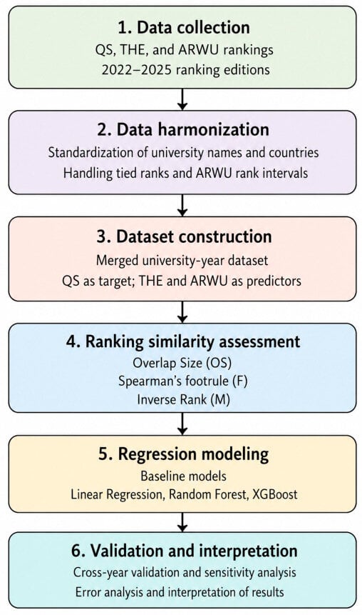
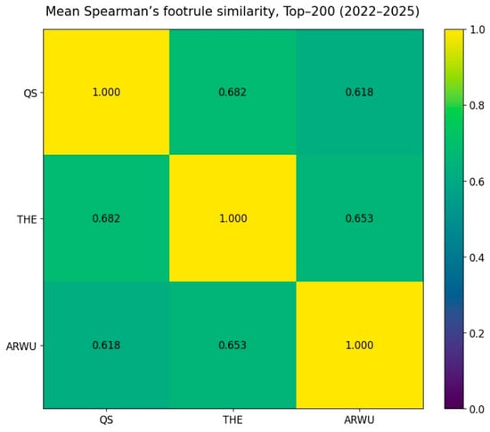
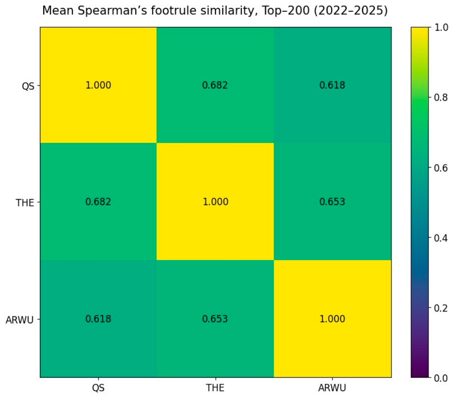
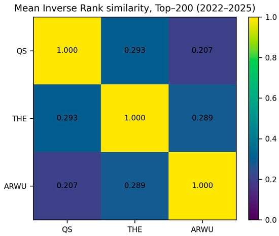
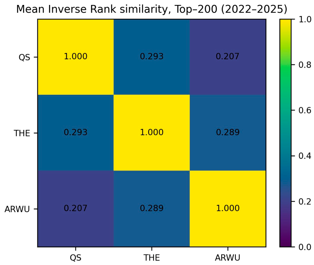
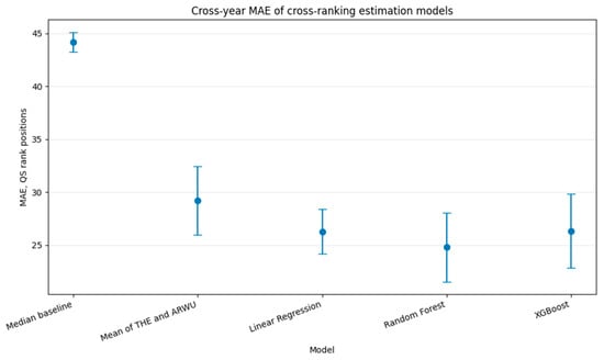
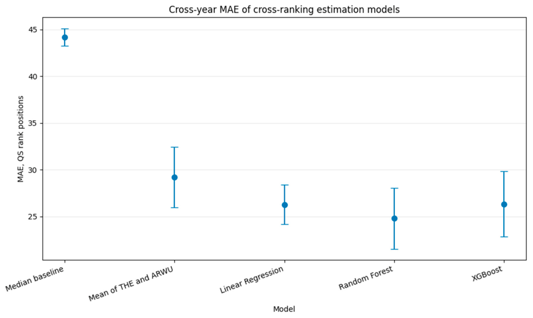
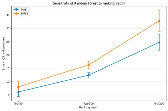
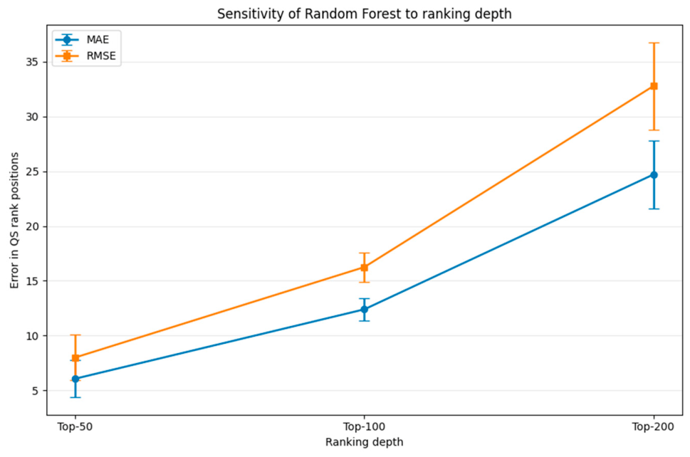
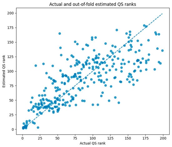
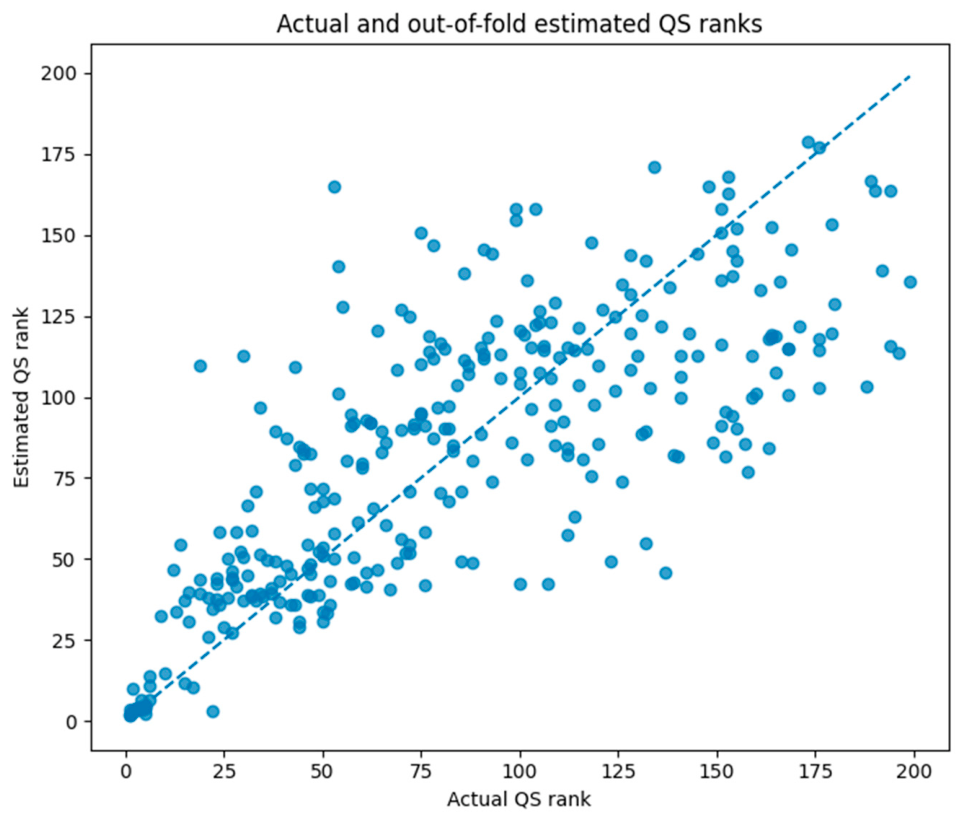
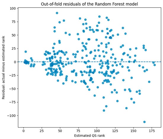
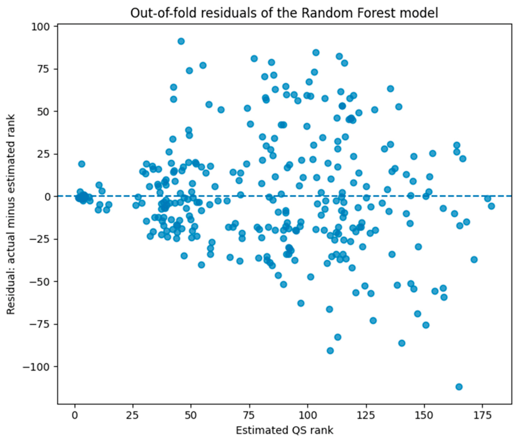

Disclaimer/Publisher’s Note: The statements, opinions and data contained in all publications are solely those of the individual author(s) and contributor(s) and not of MDPI and/or the editor(s). MDPI and/or the editor(s) disclaim responsibility for any injury to people or property resulting from any ideas, methods, instructions or products referred to in the content. |
© 2026 by the authors. Licensee MDPI, Basel, Switzerland. This article is an open access article distributed under the terms and conditions of the Creative Commons Attribution (CC BY) license.