


Abstract
Forests cover nearly one-third of the Earth’s land surface and are subject to increasing anthropogenic pressure, including unauthorised construction, infrastructure expansion, and habitat fragmentation. Detecting buildings concealed beneath forest canopy is essential for environmental monitoring and territorial surveillance, yet optical satellite imagery fails under persistent cloud cover and dense vegetation, and no existing approach provides reliable detection across contrasting forest ecosystems. We address this gap by proposing a hybrid SAR-based detection framework that combines twelve physically interpretable Scattering-Informed SAR Features (SISF)—derived from electromagnetic scattering theory across amplitude, polarimetric, temporal, and texture dimensions—with a universal Convolutional Neural Network, integrated through probability-level fusion with isotonic regional calibration. Rather than relying on individual feature thresholds, the framework identifies buildings through their characteristic multidimensional scattering signature—a combination that remains discriminative across biomes where any single SAR descriptor would fail. The framework was evaluated on a novel 7721-object multi-biome benchmark spanning forest-steppe (Kazakhstan), boreal forest (Komi Republic, Russia), and tropical rainforest (Brazil, Pará). The final Fusion + Regional Calibration model achieved an overall F1-score of 0.803 on the held-out test set (N = 1545), outperforming single-model baselines by up to 17 percentage points. Regional F1-scores ranged from 0.727 (Kazakhstan) to 0.944 (Komi Republic), with detection performance remaining robust under partial canopy occlusion (F1 = 0.911, versus 0.903 for unobscured buildings). An empirical inverse relationship between hard negative proportion and detection F1-score was identified within each biome, with the 28–35% proportions present in our sampled regions reported as a preliminary observation rather than a generally optimal range—a dataset design finding not previously reported in the literature. The proposed framework provides a physically interpretable solution for SAR-based building detection under forest canopy, demonstrating consistent performance across three contrasting forest biomes, with direct applications to environmental monitoring and territorial surveillance in forested regions.
1. Introduction
Accurate detection of buildings located within forested environments is an important task for environmental monitoring, infrastructure inventory, land-use management, and the identification of unauthorised anthropogenic activities in remote territories [1]. In regions where dense vegetation obscures the ground surface, conventional remote sensing approaches fail to provide reliable information about the spatial distribution of structures—yet it is precisely in these environments that uncontrolled construction poses the greatest threat to ecological integrity and forest conservation.
Optical satellite imagery has traditionally been the primary source of information for building extraction and land-cover mapping [2]. However, optical observations are fundamentally limited by cloud cover, atmospheric conditions, illumination variability, and seasonal vegetation changes. These limitations become especially critical in tropical forests, where persistent cloudiness can prevent optical acquisition for months at a time, and in high-latitude territories, where winter illumination conditions severely constrain observation windows. More fundamentally, buildings located beneath forest canopies may remain completely invisible in optical imagery regardless of spatial resolution, because the sensor cannot penetrate the overlying vegetation.
Synthetic Aperture Radar (SAR) provides a physically motivated alternative for monitoring forested territories [3]. Unlike optical systems, SAR actively illuminates the surface with microwave energy and records the backscattered signal, which penetrates cloud cover, operates independently of daylight, and interacts with the structural properties of both vegetation and underlying objects. The Sentinel-1 mission has made SAR data globally accessible at no cost, with systematic dual-polarisation observations at 10 m spatial resolution updated every six days—a temporal and spatial configuration well suited for large-scale operational monitoring [4].
The physical basis for SAR-based building detection under forest canopy lies in the differential scattering behaviour of vegetation and anthropogenic structures. Forest canopies are dominated by volume scattering—multiple interactions of the radar signal with branches, leaves, and tree crowns that depolarise the signal and produce characteristic temporal variability as vegetation phenology evolves through the seasonal cycle [5]. Buildings, by contrast, generate surface scattering from flat rooftops and double-bounce reflections from orthogonal wall-ground interfaces, producing stronger co-polarized returns, greater polarisation contrast, temporal stability across seasons, and locally organised texture patterns in the SAR image. These physically grounded differences provide the signal basis for detection—but their magnitude and optimal discriminative threshold vary substantially across different forest biomes, soil moisture regimes, acquisition geometries, and building sizes.
This variability has a fundamental consequence: no single SAR descriptor can serve as a universal building indicator across contrasting forest environments. A building in tropical rainforest and a building in boreal taiga may produce entirely different values of any individual SAR variable, yet both reveal their presence through a characteristic multidimensional scattering signature when amplitude, polarimetric, temporal, and texture dimensions are considered jointly. Rather than relying on fixed thresholds for individual SAR variables, the proposed framework learns multidimensional combinations of complementary scattering descriptors that remain informative across contrasting forest environments.
This principle motivates the two core architectural choices of the proposed framework. The XGBoost classifier operates on twelve physically interpretable SAR features—termed Scattering-Informed SAR Features (SISF)—learning multivariate combinations that characterise building presence across contrasting forest environments rather than applying fixed thresholds to individual variables [6]. In parallel, a universal Convolutional Neural Network receives raw pixel SAR image patches and learns spatial context—roof geometry, wall edges, structural transitions—that is invisible to aggregated polygon statistics. The two models therefore perceive fundamentally different representations of the same object: XGBoost sees the physics, CNN sees the geometry. Their probability-level fusion exploits this complementarity, recovering buildings that each model misses independently and suppressing false alarms that each model generates independently.
The framework was evaluated across three contrasting forest biomes: forest-steppe in northern Kazakhstan, boreal taiga in the Komi Republic of Russia, and tropical rainforest in the Pará state of Brazil. These regions represent the full gradient of forest-induced detection difficulty—from partial canopy cover with moderate volume scattering to dense multi-layer tropical canopy that largely masks surface-level radar contributions. Validation across this gradient provides a rigorous test of whether physically grounded SAR representations generalise across fundamentally different scattering environments without region-specific recalibration.
The main contributions of this study are as follows:
- We introduce the SISF descriptor set—a compact set of twelve physically interpretable Sentinel-1 descriptors derived from electromagnetic scattering theory, capturing backscatter intensity, polarisation contrast, temporal stability, and spatial texture. Unlike purely data-driven feature sets, SISF represents each object as a multidimensional scattering portrait rather than a collection of individually thresholded variables, establishing a direct physical link between observed radar responses and the structural properties of anthropogenic objects under forest canopy.
- We propose a hybrid detection framework combining XGBoost classification on SISF descriptors with a universal CNN trained on SAR image patches, integrated through probability-level fusion with isotonic calibration [7]. The two models capture complementary representations—physical feature combinations and spatial patch context—achieving an overall F1-score of 0.803 on the held-out test set, outperforming each individual model by up to 17 percentage points.
- We construct a multi-biome SAR benchmark comprising 7721 annotated objects across three contrasting forest ecosystems—forest-steppe (Kazakhstan), boreal forest (Komi Republic), and tropical forest (Brazil)—using a structured Hard-Negative Sampling strategy in which 28–47% of negative samples represent objects with radar signatures similar to buildings.
- We demonstrate empirically that the proportion of hard negative samples critically affects detection stability, observing a monotonic inverse relationship within each of the three biomes; the 28–35% proportions present in our sampled regions are reported as a preliminary observation—a quantitative finding that provides practical guidance for SAR dataset design in forested environments and has not been previously reported in the literature.
The remainder of this paper is organised as follows. Section 2 reviews related work on SAR-based building detection, machine learning and deep learning approaches for SAR analysis, and physical interpretability. Section 3 describes the study areas, data acquisition, dataset construction, SISF feature design, and the hybrid detection framework. Section 4 presents the experimental results across all evaluated methods and biomes. Section 5 discusses the findings in the context of the identified research gaps. Section 6 provides the conclusions.
2. Related Work
2.1. SAR-Based Building Detection
Building detection from SAR imagery has been an active research area for more than two decades. Unlike optical sensors, SAR systems operate independently of daylight conditions and are largely unaffected by cloud cover, making them particularly suitable for monitoring remote and densely vegetated regions. Early approaches relied on threshold-based analysis of radar backscatter, constant false alarm rate (CFAR) detectors, shadow analysis, Hough transforms, and contextual geometric information to identify buildings in high-resolution SAR imagery [8]. These methods demonstrated the feasibility of SAR-based building extraction but were often sensitive to imaging geometry, speckle noise, and scene complexity.
As SAR spatial resolution improved, more sophisticated approaches exploited multi-aspect observations, structural characteristics, and contextual descriptors of man-made objects. Multi-view SAR imagery improved detection reliability by providing complementary information from different acquisition geometries [9]. However, the strong dependence of radar signatures on viewing angle, vegetation cover, and local topography remained a persistent challenge.
A critical limitation of the existing literature is its near-exclusive focus on open urban environments [8,10,11,12]. Buildings in urban scenes produce strong, largely unobstructed double-bounce and surface scattering contributions that are relatively straightforward to detect [13]. The detection of buildings located within or adjacent to dense forest canopies presents a fundamentally different problem: vegetation volume scattering partially or fully masks the building-related backscatter components, and the optimal feature values for detection vary substantially across different forest types [5]. This challenge has received comparatively little attention in the published literature, motivating the cross-biome approach developed in the present study [14].
2.2. Detection of Structures Beneath Forest Canopy
Although building detection under dense vegetation has received limited attention in the mainstream SAR remote-sensing literature, a closely related problem has been studied extensively in archaeological prospection, where the goal is to detect man-made structures concealed by forest canopy. This body of work provides directly relevant physical insight. The ability of a radar signal to penetrate vegetation (foliage penetration, FoPen) increases at lower frequencies, and P- and L-band systems are generally preferred for sub-canopy sensing [15]. In practice, however, the historical sub-canopy literature has relied almost exclusively on airborne campaigns, whose coverage is limited in extent and costly to repeat. Spaceborne long-wavelength observation has only recently become available: the ESA Biomass mission (P-band) was launched in 2025 and delivers forest products at 50–200 m resolution, a scale designed for biomass rather than for individual structures, while the NASA–ISRO NISAR mission (L-band) also reached orbit in 2025 and its archive is only beginning to accumulate. For operational monitoring of buildings—objects on the order of tens of metres—across large and repeatedly observed territories, Sentinel-1 C-band therefore remains the only freely available source combining 10 m resolution, a 6–12 day revisit interval and a decade-long global archive. Establishing what can be achieved at C-band is consequently of direct practical relevance, and several studies have demonstrated that structures beneath forest canopy can also be detected at the shorter C-band wavelength. Garrison et al. [16] used airborne C-band AIRSAR data to map ancient Maya settlements beneath jungle canopy in Guatemala, deriving elevation information that revealed structures otherwise obscured by vegetation. Broader reviews of SAR archaeology [17] document a range of scattering mechanisms relevant to sub-canopy targets—surface scattering, double-bounce from walls and vertical faces, and volume scattering from vegetation—that mirror the physical basis of the features used in the present study.
Of particular relevance, recent work has shown that even C-band Sentinel-1—nominally considered inadequate for foliage penetration—can reveal structures beneath forest canopy. Michenot et al. [18] identified Maya ruins covered by jungle using multi-orbit Sentinel-1 acquisitions, arguing that the presence of a sub-canopy structure increases the local anisotropy of the scene, whether through partial penetration and double-bounce returns from the structure itself or through canopy deformation reproducing the underlying shape. This finding is central to the present work: it establishes that C-band SAR retains exploitable sensitivity to concealed structures, and it motivates our use of multi-temporal, polarimetric, and texture features to capture these subtle signatures across contrasting forest biomes. Our study differs from this archaeological literature in aim and scale—we target contemporary buildings, use a supervised hybrid machine-learning framework, and validate across three biomes rather than a single site—but shares its underlying physical rationale.
2.3. Machine Learning Approaches for SAR Analysis
The growing availability of Earth observation data stimulated the application of machine learning algorithms to SAR image interpretation. Feature-based classifiers such as Support Vector Machines (SVM), Random Forests (RF), Gradient Boosting, and XGBoost have demonstrated strong performance in SAR classification and object detection tasks by exploiting statistical, textural, polarimetric, and temporal descriptors [6,19,20].
Machine learning approaches offer important advantages for SAR analysis: they can model nonlinear relationships between radar-derived variables and target classes, require substantially fewer training samples than deep learning models, and—when physically meaningful features are used—provide interpretable decision boundaries [3]. However, the performance of feature-based approaches depends critically on the quality and physical relevance of the selected input variables.
A recurring limitation in the machine learning literature is the use of large, automatically generated feature sets without explicit grounding in electromagnetic scattering theory [21]. Features selected through statistical correlation or wrapper methods may achieve high accuracy in a specific training region while failing to generalise across different vegetation types, seasonal conditions, or acquisition geometries [3]. This observation directly motivates the physically grounded feature selection approach proposed in the present study, in which all twelve input descriptors are derived from established electromagnetic scattering principles rather than from statistical analysis of training data.
2.4. Deep Learning for SAR Building Detection
Recent advances in deep learning have significantly transformed SAR image analysis. Convolutional Neural Networks (CNNs), encoder–decoder architectures such as U-Net, and transformer-based models have demonstrated state-of-the-art performance in building extraction, semantic segmentation, change detection, and object recognition tasks [10,12,14]. CNN-based approaches automatically learn hierarchical spatial representations directly from SAR image patches, capturing complex local patterns that are difficult to encode using handcrafted descriptors.
Several studies have successfully applied deep learning for building footprint extraction, newly constructed building detection, and urban change monitoring using Sentinel-1 and very-high-resolution SAR datasets [11,22,23]. Hybrid frameworks combining CNNs with physically interpretable components have demonstrated further improvements: Huang et al. [21] proposed a physics-guided and injected learning framework (PGIL) that embeds physical scattering knowledge into CNN training through an unsupervised surrogate task, achieving improved generalisation with limited labeled data. Zhang et al. [24] demonstrated that polarimetric concept bottleneck models with Kolmogorov–Arnold Networks can achieve competitive classification accuracy while maintaining physically meaningful interpretability. Xu et al. [25] introduced physical attribute priors into incremental SAR target recognition, demonstrating that physically stable representations reduce catastrophic forgetting in sequential learning scenarios.
Despite these advances, most deep learning models for SAR building detection function as black-box systems that provide limited physical explanation of their predictions [3]. Moreover, nearly all published models are developed and validated within a single geographic region [11,12,22], leaving their transferability across contrasting forest ecosystems largely unexplored.
2.5. Physical Interpretability and Cross-Biome Transferability
A growing body of research has recognised that physically interpretable representations derived from radar scattering mechanisms can improve both model transparency and transferability [26,27]. Physically informed feature engineering establishes explicit connections between SAR observations and the structural properties of observed objects—connections that remain valid across different environmental conditions because they are grounded in electromagnetic physics rather than regional statistics.
Studies investigating spatial transferability have consistently shown that purely data-driven models degrade substantially when applied to regions differing from their training environments [3,28]. Variations in vegetation structure, moisture regime, canopy density, and acquisition geometry alter SAR backscatter distributions, causing models optimised for one biome to fail in another. This challenge is particularly acute for building detection under forest canopy, where the contrast between building-related and vegetation-related scattering varies dramatically between tropical rainforest, boreal taiga, and forest-steppe environments.
The transferability challenge is further compounded by the absence of a single universally discriminative SAR descriptor: absolute backscatter values, polarisation ratios, and texture statistics are all conditioned on vegetation type, canopy density, seasonal phenology, and acquisition geometry, rendering fixed detection thresholds inapplicable across biomes. This observation motivates a feature engineering strategy grounded in electromagnetic scattering theory rather than regional statistics—the conceptual foundation of the SISF framework proposed in this study.
Although considerable progress has been achieved in both interpretability [21,24,25] and transferability [26,27,28] research, these two directions remain largely disconnected in the context of SAR-based building detection under forest canopy. The present study addresses this gap by integrating physically interpretable SAR descriptors with hybrid machine learning across three contrasting forest biomes, providing the first cross-biome benchmark for this task.
3. Materials and Methods
3.1. Study Areas
Three geographically and ecologically distinct forest regions were selected to represent contrasting vegetation structures, canopy densities, and SAR scattering regimes (Figure 1). The regions span a gradient of increasing canopy density and detection difficulty, from forest-steppe through boreal taiga to tropical rainforest.
Figure 1.
Geographical locations of the three study areas used for cross-biome SAR-based building detection. Sentinel-1 IW GRD imagery (VV+VH polarisation, 10 m spatial resolution) was acquired across three contrasting forest biomes: (a) Kazakhstan—forest-steppe and foothill forest; (b) Komi Republic—boreal forest (taiga); (c) Brazil (Pará)—tropical forest (Amazon). Stars indicate the locations of building clusters used for model training and validation.
Kazakhstan (Forest-Steppe Zone). The study area comprises forest and forest-steppe tracts in northern and eastern Kazakhstan (centroid: 73.12° E, 52.25° N; bounding box: 62.65–84.00° E, 49.65–54.08° N). Sampling was carried out in three separate forest massifs: two in the northern forest-steppe belt (approximately 64.0–72.0° E) and one in the eastern foothill forest zone (approximately 82.5–83.9° E), comprising both forest under protected-area management and adjoining forest land outside formally designated protected-area boundaries. The landscape is characterised by discontinuous birch and pine forest interspersed with open grassland and agricultural land, typical of the Eurasian forest-steppe transition zone. Canopy height ranges from 8 to 10 m with relatively low canopy closure, resulting in partial C-band SAR penetration to underlying structures. This region represents the lowest detection difficulty in the benchmark, as partial double-bounce contributions from building walls remain detectable beneath the sparse canopy.
Komi Republic, Russia (Boreal Forest Zone). The study area is located in the Komi Republic of northwestern Russia (centroid: 55.11°E, 64.34° N; bounding box: 48.90–62.03° E, 60.00–66.45° N), encompassing intact boreal taiga representing one of Europe’s largest remaining areas of primary forest [29]. Dense continuous stands of spruce and fir reach canopy heights of 15–20 m with high canopy closure, substantially attenuating C-band SAR penetration to underlying structures. This region represents intermediate detection difficulty.
Brazil (Tropical Rainforest Zone). The study area is located in the state of Pará within the Brazilian Amazon basin (centroid: 57.98° W, 1.29° S; bounding box: 65.83–50.87° W, 3.29° S–0.16° N). The multi-layered tropical rainforest canopy, with heights of 25–35 m and year-round leaf cover, produces dominant volume scattering that largely masks double-bounce contributions from concealed structures. This region represents the highest detection difficulty in the benchmark.
3.2. SAR Data Acquisition
All SAR imagery was acquired from the Sentinel-1 constellation operated by the European Space Agency. Sentinel-1 carries a C-band synthetic aperture radar operating at 5.405 GHz (wavelength ≈ 5.6 cm), providing all-weather, day-and-night imaging capability. Data were acquired in Interferometric Wide (IW) swath mode and processed to Ground Range Detected (GRD) format at 10 m spatial resolution. Dual-polarisation VV and VH channels were used: VV backscatter is primarily sensitive to surface roughness and double-bounce contributions from vertical structures, while VH cross-polarisation reflects volume scattering from vegetation canopies.
Multi-temporal SAR time series were acquired over the peak vegetation period (June–September 2025), corresponding to the season of maximum canopy density and photosynthetic activity across all three study regions. This acquisition window was deliberately selected as the most challenging detection scenario: at peak vegetation, canopy density is maximised, volume scattering from vegetation is strongest, and the contrast between building-related and vegetation-related backscatter is most suppressed. For the Brazilian Amazon, year-round leaf cover makes this period representative of operational conditions; for Kazakhstan and Komi, the fully foliated June–September window represents the worst-case detection scenario—a conservative design choice that avoids overestimating framework performance under more favourable (leaf-off) phenological conditions. Under the applied filters (IW mode, descending orbit, dual VV/VH polarisation), the number of Sentinel-1 GRD scenes acquired over the window was 185 for Kazakhstan, 250 for Brazil, and 160 for Komi. Only descending orbit acquisitions were used. This choice was dictated primarily by data availability: over the study window the ascending-orbit archive comprises 7 scenes for Kazakhstan and none at all for Komi, against 95 for Brazil, so no ascending-based composite could be constructed consistently across the three regions. Restricting the analysis to the descending pass therefore guarantees a uniform acquisition geometry for every region, which is a prerequisite for the cross-biome comparison reported in Section 4.3. This restriction is also physically motivated: ascending and descending passes illuminate the scene from opposite azimuths, and the double-bounce return from building walls depends strongly on the orientation of the wall relative to the look direction. Combining both pass directions within a single median composite would therefore average over dissimilar scattering geometries and dilute precisely the signal that the proposed framework exploits. All preprocessing was performed within Google Earth Engine [30], including thermal noise removal, radiometric calibration, and terrain correction using the SRTM digital elevation model. Backscatter intensities were converted to the logarithmic decibel (dB) scale via ; all SAR features were computed in the dB domain. No radiometric normalisation with respect to the local incidence angle was applied, and acquisitions from all available relative orbits within the selected pass direction were combined in the median composite; the potential influence of incidence-angle variation is noted as a limitation in Section 5.5. Amplitude, polarimetric, and texture features were derived from a median composite of all available scenes, suppressing residual speckle and scene-to-scene radiometric variability; temporal features (VV_temporal_std, VV_temporal_range) were computed directly from the full image stack to preserve seasonal backscatter dynamics.
The polarimetric features were computed in the dB domain: VV_minus_VH as the difference VVdB − VHdB and VV_div_VH as the ratio VVdB/VHdB. Gray-Level Co-occurrence Matrix (GLCM) texture features (GLCM_ASM, GLCM_contrast, GLCM_entropy, GLCM_homogeneity) were computed on the median VV image (dB) using the Google Earth Engine glcmTexture operator with a neighbourhood size parameter of 3, corresponding to a pixel window ( m at 10 m resolution). Prior to texture computation, the VV image was linearly rescaled from the dB range to and quantized to 8-bit integers (256 gray levels); the operator averages the co-occurrence statistics over the four principal directions (, , , ) at unit pixel offset, yielding rotation-invariant texture descriptors. A boundary noise mask was applied ( dB, dB). No further normalisation was applied to the SAR feature values prior to model training, with the exception of standardisation (zero mean, unit variance) applied to the input of the logistic regression baseline.
3.3. Reference Data and Dataset Construction
Building footprints were obtained from OpenStreetMap (OSM) [31], a global collaborative geographic database providing freely available building polygon data; the OSM building layer was retrieved in June 2025 within a GIS environment (QGIS and ArcGIS Pro).
OSM was selected in preference to machine-learning-derived global building products, such as the recently released GlobalBuildingAtlas (GBA) [32], for three reasons specific to the present task. First, and most importantly, such products are generated by learning-based pipelines applied to optical satellite imagery—GBA is derived from PlanetScope acquisitions—and are therefore expected to systematically under-represent precisely the target class of this study: structures that are wholly or partially invisible in optical imagery because they are concealed by forest canopy. Using an optically derived product as reference would introduce a canopy-dependent labelling bias correlated with the very phenomenon under investigation. Second, OSM building polygons originate from human survey and interpretation and are thus methodologically independent of remote-sensing-derived predictions; using a model-generated product as ground truth for training another detector would propagate the errors of the source model into our labels.
Third, the completeness limitations of OSM—which are indeed more pronounced in parts of South America—were addressed directly in this study through exhaustive manual verification and geometric correction of every candidate footprint against high-resolution optical imagery, as described below, rather than by substituting an alternative automated source. We note that global products such as GBA remain valuable for large-scale deployment, and Section 5.5 discusses their potential role in extending reference coverage. The forest extent used to delimit each study area was derived from the ESA WorldCover 10 m land-cover product [33], which is based on Copernicus Sentinel-1 and Sentinel-2 data. The tree-cover and vegetated classes were retained as the forest mask, while built-up areas and settlements falling inside candidate polygons were excluded by manual inspection so that only genuine forested terrain remained. Each OSM building polygon intersecting the study area forest mask was used to define a candidate positive (Building) sample.
Every candidate building was subsequently verified and refined manually against high-resolution optical satellite imagery. To avoid geolocation inconsistencies arising from inter-sensor parallax (image shift), a single high-resolution source (Google Satellite) was used as the primary geometric reference for all footprint editing; building outlines were corrected in shape and position, and objects that could not be confirmed as buildings were removed. Editing and attribute entry were performed in ArcGIS Pro (educational license) and QGIS. This manual verification step ensured that every retained positive sample corresponds to a real, correctly georeferenced structure. For each labeled object, a pixel SAR patch was extracted centered on the object centroid, yielding a two-channel input array of normalised VV and VH backscatter values. A spatial buffer of 20 m was applied around each building footprint to account for geolocation uncertainty between OSM vector data and Sentinel-1 imagery—a known systematic offset of up to 10–15 m in IW GRD products—and to avoid labelling ambiguity at parcel boundaries.
The final annotated dataset comprises 7721 objects distributed across the three study regions, as summarised in Table 1. The number of buildings differs between regions because the density of structures within forested terrain is an intrinsic property of each landscape rather than a controllable design parameter. Rather than artificially equalising the sample counts—which would misrepresent the natural prevalence of forest-embedded buildings—we retained all verified structures within comparably forested areas, so that each regional subset reflects the true building density of its biome.
Table 1.
Dataset composition by study region.
3.4. Hard-Negative Sampling Strategy and Sample Annotation
A key methodological contribution of this study is the structured stratification of non-building samples by visual difficulty. Naive random sampling of non-building locations yields an unrealistically easy classification problem dominated by spectrally distinct forest and water pixels, failing to reflect the operational challenge of the task.
Non-building samples were divided into two strata. Easy negatives consisted of land-cover types spectrally distinct from buildings in SAR imagery: closed forest canopy, bare agricultural soil, water bodies, and open grassland. Hard negatives consisted of objects producing radar backscatter signatures similar to buildings, including gravel roads, open quarries, anthropogenic clearings, and specularly reflecting water surfaces.
The two strata were constructed by different procedures. Easy negatives were generated by sampling locations within the ESA WorldCover forest and bare-ground classes, away from any OSM building footprint, so that these samples fall on spectrally unambiguous vegetated or open terrain. Hard negatives, by contrast, were annotated entirely manually: an analyst visually inspected high-resolution optical imagery and digitized individual non-building objects that produce building-like radar returns—gravel and paved roads, railways, riverbanks and specular water surfaces, open quarries, sand and rocky surfaces, and cleared industrial sites where the topsoil has been removed. Each hard negative was tagged with the type of the nearest confusing object (water edge, road, settlement, industrial, or railway). This manual curation ensures that the hard negative stratum reflects genuine operational sources of false positives rather than arbitrary background locations.
The proportion of hard negatives within the negative class differed across regions: 28% in Komi, 33% in Brazil, and 47% in Kazakhstan, reflecting landscape heterogeneity specific to each biome. The elevated hard negative proportion in Kazakhstan reflects the high density of spectrally ambiguous non-building objects in the forest-steppe environment, where roads, quarries, and disturbed surfaces are common.
Each building sample was additionally annotated with two auxiliary attributes to enable fine-grained analysis of detection difficulty. Both attributes were assigned by manual visual interpretation of high-resolution optical reference imagery by a single analyst. The canopy occlusion level was assigned based on the proportion of the building footprint covered by forest canopy as visible in high-resolution optical reference imagery: open (no canopy cover), partially occluded (canopy covering 30–70% of the footprint), and fully occluded (more than 70% of the footprint beneath canopy). Fully occluded buildings are not directly visible on any single optical image; their presence was confirmed by cross-referencing several independent high-resolution sources (Google, Bing, Yandex and Maxar imagery) acquired at different dates. For the Kazakhstan and Komi sites, where the canopy is seasonally deciduous, leaf-off winter acquisitions provided an additional confirmation route in which the structure becomes momentarily visible; this route is not available for the Brazilian site, where the evergreen tropical canopy provides no leaf-off window, and confirmation there relied solely on multi-source and multi-date cross-referencing. It should be emphasised that these additional sources were used only to confirm the existence of a structure; all footprint geometry was digitized against the single geometric reference described in Section 3.3, so that no inter-sensor positional bias was introduced. This category is deliberately small, as a structure was retained only where its presence could be positively confirmed by at least one independent observation. The spatial position relative to the forest boundary was classified as forest edge (building centroid located within 50 m of the forest boundary) or forest interior (centroid located more than 50 m inside the forest boundary). These auxiliary annotations were not used as model inputs but served exclusively for post-hoc stratified evaluation of detection performance, as reported in Section 4.6. All annotations were recorded in a structured attribute table in ArcGIS Pro using controlled value domains for the occlusion level, forest position, and nearest-object type, which constrained each field to a predefined set of categories and thereby enforced labelling consistency across the three regions.
3.5. Scattering-Informed SAR Features (SISF)
Feature selection was not performed empirically but was derived directly from electromagnetic scattering theory. The proposed SISF set comprises twelve physically interpretable descriptors organized into four complementary groups, each capturing a distinct aspect of microwave interaction with vegetation and anthropogenic structures (Table 2).
The physical basis relies on differential scattering behaviour of forest vegetation and buildings. In forested environments, SAR returns are dominated by volume scattering caused by multiple interactions of the radar signal with branches, leaves, and tree crowns [5]. Buildings, on the other hand, produce stronger surface scattering and double-bounce reflections due to flat surfaces and orthogonal geometric elements such as walls and roofs [13]. Four complementary feature groups were constructed to capture these differences.
Amplitude features (VV_mean, VH_mean, VV_stdDev, VH_stdDev) characterize the mean intensity and spatial variability of co- and cross-polarized backscatter. VV polarisation is sensitive to surface and double-bounce scattering, while VH is strongly influenced by volume scattering within the vegetation canopy [34].
Polarimetric features (VV_minus_VH, VV_div_VH) quantify the contrast and ratio between co-polarized and cross-polarized returns. Buildings typically exhibit a stronger VV response relative to VH due to enhanced double-bounce scattering, whereas forested areas tend to produce more balanced polarisation signatures dominated by volume scattering [13].
Temporal features (VV_temporal_std, VV_temporal_range) capture the stability of VV backscatter over the seasonal observation cycle. Buildings represent permanent structures with stable electromagnetic properties, while vegetation undergoes phenological changes that introduce temporal variability in SAR backscatter [35].
Texture features (GLCM_ASM, GLCM_contrast, GLCM_entropy, GLCM_homogeneity) are derived from the Gray-Level Co-occurrence Matrix [36] and describe the spatial organisation of local backscatter patterns. Forest canopies generate complex, irregular spatial patterns, whereas buildings introduce geometric regularity and abrupt transitions in local backscatter values. GLCM-based texture descriptors have been shown to provide discriminative information in Sentinel-1 C-band applications over vegetated terrain: they have been applied to unsupervised burned-area detection in Mediterranean forest ecosystems [37] and, in combination with dual-polarisation VV/VH backscatter and tree-ensemble classifiers, have been reported to yield measurable gains in classification accuracy for SAR-based mapping tasks [38]. These results support the inclusion of GLCM descriptors for characterising building-induced spatial anomalies under forest cover.
Figure 2 illustrates these scattering differences for one representative building object from each biome, demonstrating that while raw SAR backscatter provides ambiguous evidence of building presence, polarimetric contrast and GLCM-based texture descriptors reveal physically interpretable anomalies that persist across contrasting forest environments.
Figure 2.
Representative SAR patch visualisation for one partially occluded building located within forest interior (Forest_pos = inside, Occlusion = partial) from each of the three study biomes. Each row corresponds to one annotated building object. Columns show, from left to right: (1) Sentinel-2 optical RGB composite at 10 m resolution—the building is barely distinguishable within the forest canopy; (2) normalised Sentinel-1 VV backscatter—a localised amplitude anomaly is visible at the building location; (3) normalised Sentinel-1 VH backscatter—cross-polarisation response reflects the transition between volume scattering dominated forest and the building surface; (4) VV/VH polarimetric ratio—elevated values indicate double-bounce scattering dominance at the building footprint; (5) GLCM Contrast map computed from a sliding pixel window over the VV channel—the building boundary produces a sharp localised texture anomaly that is clearly separable from the surrounding forest canopy. The progression from left to right illustrates the physical rationale for the SISF feature framework: while optical and raw SAR imagery provide ambiguous building evidence, texture-based and polarimetric descriptors reveal physically interpretable scattering anomalies that persist across contrasting forest environments.
No single SISF descriptor can reliably identify buildings across different forest biomes, as absolute backscatter values depend on vegetation type, canopy density, soil moisture, and acquisition geometry. The methodology therefore represents each object as a twelve-dimensional SISF vector and relies on machine learning to identify complex multivariate relationships with building presence across contrasting environments.
Table 2.
Scattering-Informed SAR Features (SISF) and their physical interpretation.
Figure 3 illustrates the univariate distributions of all twelve SISF descriptors for building and non-building classes across the combined three-region dataset, providing visual confirmation of the physical discriminability underlying each feature group.
Figure 3.
Univariate distributions of all twelve SISF descriptors for building (coloured) and non-building (grey) classes across the combined three-region dataset (N = 7721). Dashed lines indicate class means; denotes the absolute difference between means. Colours indicate feature groups: amplitude (orange), polarimetric (blue), temporal (green), texture (purple).
The distributions confirm that no single SISF descriptor provides universal separation between building and non-building classes across all three biomes. GLCM_contrast exhibits the largest mean separation (), consistent with its physical interpretation as a measure of abrupt backscatter transitions at building edges—a property that persists regardless of forest type or acquisition geometry. Amplitude descriptors (VV_mean, VH_mean) show moderate separation ( and dB respectively), reflecting the expected double-bounce enhancement at building walls, but with substantial distributional overlap driven by cross-regional variability in absolute backscatter levels. GLCM_ASM exhibits near-zero mean separation (), indicating that its discriminative contribution operates through distributional shape differences and multivariate interactions within the twelve-dimensional SISF space rather than univariate thresholding—consistent with its lower but non-negligible feature importance ranking (XGBoost: 0.059, Random Forest: 0.061). Collectively, these distributions motivate the multidimensional SISF representation and the use of nonlinear ensemble classifiers capable of exploiting complex feature combinations.
3.6. Hybrid Detection Framework
The proposed framework integrates two complementary detection pathways—a feature-based XGBoost classifier operating on SISF descriptors and a universal Convolutional Neural Network operating on SAR image patches—through a probability-level fusion strategy (Figure 4).
Figure 4.
Schematic overview of the proposed hybrid detection framework combining XGBoost classification on Scattering-Informed SAR Features (SISF) and a universal CNN operating on SAR image patches, integrated through isotonic calibration and probability-level fusion with regional decision thresholds (KZ: 0.34, BR: 0.45, KM: 0.48).
3.6.1. XGBoost Classifier
The XGBoost classifier operates on the twelve-dimensional SISF feature vector extracted for each labeled object. XGBoost constructs an ensemble of decision trees sequentially, with each successive tree correcting residual errors of its predecessors [6]. The algorithm was selected for its ability to model complex nonlinear interactions among SAR-derived features, its robustness to feature-scale differences, and its natural compatibility with isotonic probability calibration.
Hyperparameters were selected via 5-fold cross-validation grid search over the following ranges: n_estimators ∈ {200, 300, 500}, max_depth ∈ {3, 4, 5, 6}, learning_rate ∈ {0.03, 0.05, 0.1}, subsample ∈ {0.8, 1.0}, and colsample_bytree ∈ {0.8, 1.0}. The selected configuration was n_estimators = 300, max_depth = 5, learning_rate = 0.05, subsample = 0.8, and colsample_bytree = 0.8, which yielded the highest held-out F1-score; results were insensitive to max_depth within (F1 varied by less than 0.002). A fixed random seed of 42 was used throughout. Class imbalance was addressed through the scale_pos_weight parameter set to the ratio of negative to positive training samples. The raw XGBoost output is a probability score for the building class.
3.6.2. Universal CNN
The CNN component operates on raw pixel SAR patches with two input channels corresponding to normalised VV and VH backscatter values. The architecture consists of three convolutional blocks with 32, 64, and 64 filters respectively, each using a convolution with ReLU activation followed by max-pooling; dropout was applied after each block (rates 0.10, 0.10, and 0.30). The feature maps were flattened and passed to a fully connected layer with 64 units, followed by a single sigmoid output neuron producing the building probability . Batch normalisation was applied within the convolutional blocks.
The CNN was trained jointly on all three study regions as a single universal model, without region-specific fine-tuning. Class imbalance was addressed through class-weighted binary cross-entropy loss, with weights set inversely proportional to class frequency. Training used the Adam optimizer (initial learning rate , reduced by a factor of 0.5 on validation-loss plateau with patience of 2 epochs) with a batch size of 32 for up to 50 epochs. Early stopping (patience of 8 epochs, monitoring validation AUC) with best-weight restoration was used for model selection, and the best checkpoint by validation performance was retained. All random seeds (Python 3.10.13, NumPy 1.24.4, and TensorFlow 2.15.0) were fixed to 42 for reproducibility. No data augmentation was applied; the model achieved its reported performance directly from the annotated patches.
3.6.3. Probability-Level Fusion and Regional Calibration
Prior to fusion, both model outputs were independently calibrated using isotonic regression [7]. Calibration is necessary because raw neural network outputs tend to be overconfident—producing probability scores concentrated near 0 and 1—making direct averaging with XGBoost probability scales mathematically inconsistent. Isotonic calibration learns a monotone non-parametric mapping from raw scores to calibrated probabilities, fitted on a dedicated held-out calibration subset (16% of the full dataset) separate from the test set to prevent data leakage.
The fused probability was computed as the arithmetic mean of calibrated CNN and XGBoost posteriors:
where and denote calibrated CNN and XGBoost probabilities, respectively. An optimal decision threshold was subsequently determined independently for each region by maximising the F1-score on the validation set, yielding regional thresholds of 0.34 (Kazakhstan), 0.45 (Brazil), and 0.48 (Komi). The substantially lower threshold required for Kazakhstan reflects the elevated proportion of hard negative samples in that region, which compresses posterior probability distributions toward the decision boundary and necessitates a lower threshold to recover true positive detections at acceptable recall levels.
3.7. Training Protocol and Evaluation Metrics
A single stratified 80/20 train–test split (fixed random seed of 42, stratification jointly by region and class label) was applied to the complete dataset of 7721 objects and used consistently for all evaluated methods, ensuring that the baseline classifiers and the proposed framework were assessed on the identical held-out test subset of 1545 objects, with proportional representation of all region–class combinations. For the proposed framework, the training portion was further subdivided—using the same stratification scheme and random seed—into training (64% of the complete dataset) and validation (16%) subsets, yielding the overall 64/16/20 partition. The validation subset served exclusively for hyperparameter tuning, early stopping of the CNN, and decision threshold optimisation; the baseline classifiers did not require a separate validation subset, as their hyperparameters were selected via 5-fold cross-validation within the training portion. The test subset was reserved for final performance evaluation and was not used during any stage of development of any model.
Model performance was evaluated using Precision, Recall, and F1-score computed on the building class, together with the absolute counts of true positives (TP), false positives (FP), and false negatives (FN). F1-score was selected as the primary evaluation metric because it accounts simultaneously for detection completeness and false alarm rate, making it appropriate for imbalanced binary classification tasks where the building class is of primary interest. All reported metrics were computed on the held-out test subset.
In addition to F1-score, Balanced Accuracy—defined as the arithmetic mean of Sensitivity (Recall on the building class) and Specificity (Recall on the non-building class)—was reported for all evaluated methods. Balanced Accuracy provides a class-imbalance-robust complement to F1-score, as it weights both classes equally regardless of their relative sample sizes [39].
4. Results
4.1. Baseline Machine Learning Models
To establish performance baselines and evaluate the discriminative capacity of the proposed SISF descriptors, three classical machine learning classifiers were trained and evaluated: Logistic Regression (LR), Random Forest (RF), and XGBoost. All models were trained on the combined three-region dataset comprising 7721 annotated objects, using the same stratified train–test split described in Section 3.7: all baselines were trained on the 80% training portion and evaluated on the identical held-out 20% test subset used for the proposed framework. Stratification was performed jointly by region and class label to preserve the regional and class-balance distribution in both subsets. Note that the baseline models were trained on the full 80% training portion, whereas the XGBoost and CNN components of the proposed framework were trained on only 64% of the data (with 16% held out for validation); any asymmetry in training data volume therefore favours the baselines.
Results are summarised in Table 3.
Table 3.
F1-scores of baseline machine learning classifiers by region.
Logistic Regression failed substantially across all three regions, achieving an overall F1-score of only 0.354. The pattern of high precision (Overall Precision = 0.644) combined with extremely low recall (Overall Recall = 0.244)—most pronounced in Komi (Precision = 0.700, Recall = 0.119, F1 = 0.203)—indicates that the linear classifier learned an overly conservative decision boundary, assigning almost all ambiguous samples to the non-building class. The large number of false negatives (FN = 408 out of 540 true buildings) confirms that a linear decision surface is fundamentally inadequate for this task. This result validates the central premise of the SISF framework: the relationship between physically interpretable SAR descriptors and the presence of anthropogenic structures under forest canopy is inherently nonlinear and cannot be captured by a linear model regardless of feature quality. Ensemble or deep learning approaches are necessary to properly exploit the discriminative information encoded in the SISF feature space.
Random Forest demonstrated substantially improved and consistent performance across all three biomes, achieving an overall F1-score of 0.642 (Precision = 0.707, Recall = 0.589, TP = 318, FP = 132, FN = 222). The F1-score range across regions was narrow (0.629–0.664), indicating that the SISF feature set captures physical properties of anthropogenic structures that remain discriminative across the three contrasting forest environments represented in the dataset—from the open forest-steppe of Kazakhstan to the dense boreal forests of Komi. This cross-biome consistency is a direct consequence of grounding the feature set in electromagnetic scattering theory rather than region-specific statistical patterns.
XGBoost achieved a comparable overall F1-score of 0.633 (Precision = 0.721, Recall = 0.565, TP = 305, FP = 118, FN = 235). Relative to Random Forest, XGBoost exhibited higher precision at the cost of lower recall—a pattern consistent with the gradient boosting mechanism [6], which progressively focuses on hard-to-classify examples and tends to assign higher confidence scores to well-supported positive predictions while withholding predictions on ambiguous samples. This conservative precision-oriented behaviour, while reducing false alarms, results in a greater number of missed buildings compared to Random Forest. Given its superior compatibility with isotonic probability calibration and its well-established performance on tabular SAR feature classification tasks in the literature, XGBoost was selected as the tabular component of the fusion framework described in Section 4.3.
4.2. Universal CNN Performance and Comparison with XGBoost
A universal Convolutional Neural Network was trained jointly on Sentinel-1 SAR image patches drawn from all three study regions. Each patch measured pixels (as described in Section 3.3). Patches contained two channels corresponding to VV and VH polarisation backscatter intensity. The full dataset was partitioned into training (64%), validation (16%), and test (20%) subsets using stratified sampling by region and class label. Class imbalance was addressed through class-weighted binary cross-entropy loss during training, with weights computed from the training subset class distribution.
Table 4 presents the precision, recall, and F1-scores of XGBoost and the universal CNN by region. Figure 5 illustrates the complementary precision-recall profiles of XGBoost and CNN Universal across all three study regions.
Table 4.
Performance of XGBoost and CNN Universal by region (decision threshold = 0.50).
Figure 5.
Precision and Recall profiles of XGBoost and CNN Universal by region (test set, N = 1545). XGBoost exhibits consistently higher precision with lower recall, while CNN demonstrates a more balanced detection profile—a complementarity that motivates the probability-level fusion strategy.
The universal CNN achieved an overall F1-score of 0.740, outperforming XGBoost by 10.7 percentage points. This improvement demonstrates that spatial information contained within SAR image patches contributes substantial discriminatory power beyond that captured by the SISF tabular descriptors alone. The relatively uniform regional performance of the CNN (F1 range: 0.726–0.763) confirms that a single model trained jointly on data from three contrasting forest biomes generalises effectively across different scattering environments without region-specific fine-tuning.
A detailed examination of the precision-recall profiles reveals a fundamentally complementary relationship between XGBoost and CNN. XGBoost consistently exhibited high precision but substantially lower recall across all regions (overall Precision = 0.721, Recall = 0.565): when XGBoost predicts a building, it is rarely wrong, but it fails to detect a large proportion of true buildings—particularly in Brazil (Recall = 0.541) and Komi (Recall = 0.542), where complex forest scattering environments produce many ambiguous SAR signatures. The CNN, conversely, demonstrated substantially higher recall (overall Recall = 0.737), detecting a greater proportion of true buildings at the cost of slightly more false positives (FP = 138 vs. 118 for XGBoost). This structural complementarity—XGBoost prioritising precision through tabular SISF descriptors, CNN prioritising recall through spatial patch context—provides the theoretical foundation for the probability-level fusion described in the following section.
4.3. Fusion of CNN and XGBoost Predictions
The complementary error profiles documented in Section 4.2 motivated a probability-level fusion strategy combining the calibrated posterior probabilities of XGBoost and the universal CNN (see Section 3.6.3 for calibration details). The fusion was evaluated in two configurations: without regional threshold optimisation (Fusion CNN + XGBoost) and with per-region decision thresholds optimised on the validation set (Fusion + Regional Calibration).
Table 5 presents the complete performance comparison across all evaluated methods, from the simplest baseline to the final calibrated fusion model. Figure 6 shows the confusion matrices for all four primary models, and Figure 7 illustrates the progressive improvement in F1-score across the full method hierarchy.
Table 5.
Overall performance comparison across all evaluated methods (test set, N = 1545).
Figure 6.
Confusion matrices for XGBoost, CNN Universal, Fusion CNN + XGBoost, and Fusion + Regional Calibration models on the held-out test set (N = 1545). Colour intensity is proportional to prediction count. The final model (d) achieves the highest true positive count (447) and lowest false negative count (93) across all evaluated methods.
Figure 7.
Progressive improvement in F1-score across the evaluated method hierarchy. Results are reported on the held-out test set (N = 1545). The method sequence follows the architectural complexity of the framework: from linear baseline (Logistic Regression) through ensemble machine learning (Random Forest, XGBoost) and deep spatial learning (CNN Universal) to the final hybrid fusion with regional calibration (Fusion + Regional Calibration).
The Fusion CNN+XGBoost model achieved an overall F1-score of 0.763, representing an improvement of 2.3 percentage points over the CNN alone and 13.0 percentage points over the XGBoost baseline. The reduction in false positives from 138 to 100—a decrease of 27.5%—confirms that XGBoost’s conservative precision-oriented predictions effectively suppress the CNN’s false alarms. The marginal increase in false negatives (142 → 145) at the standard threshold of 0.50 is consistent with the precision-recall trade-off inherent in averaging two models with different operating points.
Regional probability calibration with optimised per-region decision thresholds further improved overall performance to F1 = 0.803. This improvement was driven primarily by a substantial increase in true positives (395 → 447, +13.2%) and a corresponding reduction in false negatives (145 → 93, −35.9%), indicating that calibrated regional thresholds allow the model to recover buildings that the fixed threshold suppressed. False positives increased slightly (100 → 127), reflecting the lower decision thresholds applied in regions with high hard negative proportions.
4.4. Regional Analysis and the Role of Hard Negative Sampling
Table 6 presents the regional performance of the final Fusion + Regional Calibration model. Figure 8 illustrates the relationship between hard negative proportion and F1-score across the three biomes.
Table 6.
Regional performance of the Fusion + Regional Calibration model.
Figure 8.
Effect of hard negative proportion on detection F1-score, evaluated independently for each study region (XGBoost on SISF features; each point is the mean of 5-fold cross-validation averaged over 10 randomized runs, with shaded bands showing ±1 standard deviation). Within every region the relationship is monotonically decreasing: F1 is highest at low hard negative proportions and declines as the proportion increases. Diamond markers indicate the hard negative proportion naturally present in each regional dataset (Komi 28%, Brazil 33%, Kazakhstan 47%). The 28–35% band observed in this study reflects the proportions occurring in the sampled regions rather than a generally optimal value.
Regional performance varied substantially across biomes, ranging from F1 = 0.727 in Kazakhstan to F1 = 0.944 in Komi. While differences in forest structure and radar scattering complexity contribute to this variation—tropical forests produce intense volume scattering that partially masks building-related backscatter components, while boreal forests exhibit more homogeneous and predictable scattering regimes—the results reveal that dataset composition plays an equally critical role.
A key empirical finding of this study concerns the relationship between the proportion of hard negative samples and detection stability. Hard negatives were incorporated into all regional datasets through deliberate Hard-Negative Sampling (Section 3.4), but their proportion within the negative class differed substantially across regions: Kazakhstan contained 47% hard negatives, compared to 33% in Brazil and 28% in Komi.
The results reveal a consistent and monotonic inverse relationship between hard negative proportion and F1-score. Komi, with the lowest hard negative proportion (28%), achieved the highest F1-score (0.944). Brazil (33% hard negatives) achieved F1 = 0.790. Kazakhstan (47% hard negatives) produced the lowest regional F1-score (0.727). We caution, however, that these three regional points differ simultaneously in hard negative proportion and in biome type (forest-steppe, tropical rainforest, and boreal forest), so the regional comparison alone cannot isolate the effect of hard negative proportion from that of forest structure.
To disentangle these factors, we additionally conducted a controlled experiment in which the hard negative proportion was systematically varied from 10% to 65%within each region separately, holding the biome fixed (XGBoost on SISF features, 5-fold cross-validation averaged over 10 randomized runs; Figure 8). Under this controlled design, all three regions exhibit the same monotonically decreasing trend: F1 is highest at the lowest tested proportion (10%) and declines as the proportion increases, plateauing once easy negatives are exhausted. This within-region result confirms that the inverse relationship is driven by the hard negative proportion itself rather than solely by biome differences. We emphasize that the 28–35% band corresponds to the hard negative proportions that happened to occur in two of our three sampled regions, and does not represent a generally optimal setting; the monotonic decline indicates that, in these datasets, still lower proportions yield higher cross-validated F1. Because this observation is derived from only three regions, we regard it as a preliminary finding that should be validated on a broader set of forest environments before any proportion is recommended as generally appropriate.
The optimal decision thresholds provide additional physical insight into this relationship. Kazakhstan required a substantially lower threshold (0.34) compared to Brazil (0.45) and Komi (0.48), indicating that the calibrated fusion model must shift its operating point toward higher recall to recover buildings from a background containing a large proportion of ambiguous non-building objects. This threshold shift is a direct and interpretable consequence of the elevated hard negative proportion in the Kazakhstan dataset and represents a quantitative manifestation of the increased classification difficulty in the forest-steppe environment.
4.5. SISF Feature Importance Analysis
To assess the relative contribution of each SISF descriptor to the classification decision, feature importance scores were computed for both the XGBoost and Random Forest classifiers trained on the full three-region dataset (N = 7721). Results are presented in Figure 9. SHAP (SHapley Additive exPlanations) values were additionally computed for the XGBoost model to provide a direction-aware assessment of each feature’s influence on individual predictions (Figure 10).
Figure 9.
Feature importance scores for all twelve SISF descriptors computed from (a) XGBoost and (b) Random Forest classifiers trained on the full three-region dataset (N = 7721). Colours indicate feature groups: amplitude (orange), polarimetric (blue), temporal (green), texture (purple). GLCM_contrast ranked first in both models, consistent with the physical importance of local backscatter contrast at building boundaries.
Figure 10.
SHAP summary plot for the XGBoost classifier trained on SISF features (N = 7721). Each point represents one object; horizontal position indicates the magnitude and direction of the feature’s contribution to the model output; colour indicates the feature value (red = high, blue = low). Features are ordered by mean absolute SHAP value.
Feature importance rankings were consistent across both classifiers. GLCM_contrast ranked first in both XGBoost (importance = 0.139) and Random Forest (importance = 0.126), followed by VH_mean (XGBoost: 0.115, RF: 0.105) and VV_minus_VH (XGBoost: 0.106, RF: 0.094). Importantly, no single descriptor dominated the ranking—the importance scores were distributed across all four feature groups, with the top-ranked descriptor accounting for only 13.9% of total importance in XGBoost. This relatively uniform distribution confirms that building detection under forest canopy is an inherently multidimensional problem that cannot be reduced to a single discriminative feature, regardless of its individual informativeness.
The SHAP summary plot (Figure 10) reveals the directional structure of feature contributions within the trained model. We emphasize that these values quantify statistical associations learned by the classifier and indicate how each feature influences model output; they are consistent with, but do not by themselves prove, the underlying physical scattering mechanisms discussed below. For GLCM_contrast, high feature values produce both strongly positive and strongly negative SHAP contributions depending on object context—indicating that the model exploits contrast not as a simple threshold but as a contextual discriminator within the broader SISF feature space. VH_mean exhibits a consistent directional pattern: high cross-polarisation returns push predictions toward non-building (a pattern consistent with volume scattering dominance in dense forest canopy), while low VH_mean values support building detection. VV_temporal_std, despite its moderate importance score, shows a tight and stable SHAP distribution—reflecting its role as a reliable cross-biome discriminator whose contribution is consistent rather than context-dependent.
4.6. Analysis by Canopy Occlusion and Building Position
To assess the influence of vegetation cover on detection performance, the test set was stratified by the degree of canopy occlusion and the spatial position of buildings relative to the forest boundary. Results are presented in Figure 11, and false positive rates by negative sample type are shown in Figure 12.
Figure 11.
Detection F1-score stratified by canopy occlusion level (a) and building position relative to the forest boundary (b). Results are reported for the Fusion + Regional Calibration model on the held-out test set (N = 540 buildings). Open (n = 401) and partially occluded (n = 134) buildings achieve statistically indistinguishable F1-scores (0.903 and 0.911 respectively), confirming that SISF descriptors retain discriminability under partial canopy cover; the fully occluded stratum contains only five test objects and is therefore not reported. Forest edge buildings (n = 229, F1 = 0.932) outperform forest interior buildings (n = 311, F1 = 0.885), consistent with reduced canopy attenuation at forest margins.
Figure 12.
False positive rate for easy negatives and hard negatives across all evaluated models. Hard negatives consistently produce substantially higher false positive rates than easy negatives across all methods. The Fusion + Regional Calibration model achieves the lowest hard negative false positive rate (24.1%), representing a reduction of 12.1 percentage points relative to XGBoost alone (36.2%), while maintaining a low easy negative false positive rate of 6.5%—a fourfold difference that identifies hard negatives as the primary remaining source of classification error.
Detection performance remained robust across occlusion levels. Open buildings (n = 401) achieved F1 = 0.903 and partially occluded buildings (n = 134) F1 = 0.911—the two strata are statistically indistinguishable, with partial occlusion showing no measurable performance penalty. This result is particularly significant because it indicates that the proposed SISF framework captures scattering anomalies introduced by buildings even when the structure is partially obscured by the forest canopy. The physical interpretation is consistent with established SAR scattering theory: partial canopy occlusion does not eliminate the double-bounce backscatter component at building walls and roofs, the spatial disruption of volume scattering homogeneity, or the temporal stability contrast between permanent anthropogenic structures and seasonally variable vegetation. These physically grounded signal components, explicitly encoded in the SISF feature set, preserve discriminability even under partial occlusion conditions.
The fully occluded stratum (canopy cover > 70%) is represented by only five buildings in the held-out test subset, reflecting the deliberately conservative annotation policy described in Section 3.4: a structure was assigned to this category only when its presence could be positively confirmed by independent observations despite not being visible in any single optical image. All five were correctly detected, but a stratum of this size does not support any quantitative inference, and we therefore refrain from reporting a performance estimate for it. Whether detection degrades under continuous dense canopy—as would be expected from the attenuation of double-bounce backscatter, the weakening of volume-scattering disruption within the pixel patch, and the reduced temporal stability contrast—remains an open question that this dataset cannot answer. Quantifying the fully occluded regime would require a dedicated data collection effort targeting such structures, and possibly additional discriminative information such as InSAR coherence or higher-resolution SAR; we identify this as a priority for future work (Section 5.5).
Analysis of building position relative to the forest boundary revealed a complementary pattern. Buildings located at the forest edge (n = 229) achieved higher detection accuracy (F1 = 0.932) compared to those fully embedded within forest interiors (n = 311, F1 = 0.885). This approximately five percentage point difference reflects the reduced volume scattering interference at forest margins, where the surrounding canopy contributes less attenuation to the building-related backscatter signal. Buildings embedded within dense forest interiors are subject to stronger canopy-induced signal attenuation and greater spatial mixing of building and vegetation scattering components within the pixel patch window, increasing classification difficulty.
False positive analysis revealed that hard negatives remain the dominant source of classification error across all evaluated methods. The Fusion + Regional Calibration model produced a false positive rate of 6.5% for easy negatives compared to 24.1% for hard negatives, a fourfold difference that underscores the fundamental challenge of discriminating buildings from spectrally similar non-building objects in SAR imagery. This result confirms the importance of the Hard-Negative Sampling strategy employed during dataset construction: by explicitly including representative hard negative samples during training, the framework learns to distinguish buildings from the most challenging non-building confounders. The residual false positive rate of 24.1% on hard negatives identifies the primary direction for future improvement, potentially through the incorporation of additional discriminative features such as temporal coherence or higher-resolution SAR data.
5. Discussion
5.1. Physical Interpretability of the SISF Framework
The results indicate that physically grounded feature engineering produces representations that remain consistently discriminative across the three studied biomes [26,27]: the twelve SISF descriptors achieved consistent cross-biome performance with Random Forest (F1 range: 0.629–0.664) without any region-specific tuning—a degree of geographic robustness that purely statistical-texture features, which tend to encode region-specific backscatter distributions, rarely achieve [21].
The cross-biome consistency of SISF can be understood through the complementary contributions of its four feature groups. Temporal features (VV_temporal_std, VV_temporal_range) proved particularly important for cross-regional consistency: buildings maintain stable backscatter properties across seasons regardless of biome type, while vegetation undergoes phenological change that introduces systematic temporal variability [35]. This temporal invariance is a physics-derived property that held consistently across the three studied forest environments, making it the most regionally stable component of the SISF set. Polarimetric features (VV_minus_VH, VV_div_VH) capture the fundamental contrast between double-bounce and volume scattering, providing discrimination that is independent of absolute backscatter calibration and therefore robust to cross-regional radiometric differences [5,13]. Amplitude features (VV_mean, VH_mean and their spatial standard deviations) contribute complementary intensity-level information that, while more sensitive to acquisition geometry and soil moisture, remains informative when combined with the other groups rather than used in isolation. Texture features (GLCM_ASM, GLCM_contrast, GLCM_entropy, GLCM_homogeneity) capture the spatial organisation of local backscatter patterns—the geometric regularity of rooftops versus the chaotic structure of forest canopy—a distinction that persists across biomes because it reflects fundamental differences in surface geometry rather than regional backscatter statistics. Feature importance analysis (Figure 9) showed that GLCM_contrast ranked as the single most informative descriptor across both XGBoost (importance = 0.139) and Random Forest (importance = 0.126), a ranking consistent with the physical expectation that abrupt backscatter transitions at building edges and wall boundaries produce locally high contrast values largely absent in the spatially diffuse scattering of forest canopy. It is worth noting that the informativeness of texture is task-dependent: in Sentinel-1 burned-area mapping, GLCM-derived components have been reported to contribute comparatively little relative to backscatter-change indices [38]. This contrast is instructive rather than contradictory. Burned-area detection is fundamentally a change-detection problem, in which the informative signal is the temporal drop in backscatter following the loss of vegetation, so that texture adds little beyond the change indices. Building detection under canopy, by contrast, is a single-epoch problem in which the target is a persistent, geometrically organised structure embedded in a spatially chaotic background; here the local arrangement of backscatter is the primary discriminative cue, which is consistent with the leading rank of GLCM_contrast in our analysis. Notably, the importance distribution remained relatively uniform across all four feature groups—the top-ranked descriptor accounted for only 13.9% of total XGBoost importance—indicating that no single physical dimension alone is sufficient for cross-biome building detection.
5.2. Physical Constraints: C-Band Penetration and System Noise
The detection performance reported above is bounded by two physical constraints inherent to the sensor: limited canopy penetration at C-band, and the instrument noise floor. Both merit explicit discussion, as they determine where the proposed framework succeeds and where it fails.
Canopy penetration. Sentinel-1 operates at C-band ( cm), a wavelength at which propagation through a closed canopy is strongly attenuated: extinction by leaves and small branches is high, and the effective scattering phase centre lies within the upper canopy rather than at the ground. Longer wavelengths (L- and P-band) are consequently preferred for foliage-penetration applications [15], and C-band is often regarded as unsuitable for sub-canopy sensing. Our results should therefore not be interpreted as evidence of full canopy penetration. Two non-exclusive mechanisms can account for the building-related signal observed here, following the reasoning of Michenot et al. [18]. First, partial penetration: a fraction of the incident field reaches the structure through canopy gaps and along low-attenuation paths, producing surface and double-bounce returns that survive two-way attenuation. Second, canopy conformity: even without penetration, the presence of a structure perturbs the geometry and vertical distribution of the overlying canopy, so that the upper-canopy scattering layer partially reproduces the underlying shape and locally breaks the statistical isotropy of the forest.
This interpretation is consistent with the occlusion-stratified results of Section 4.6. Detection is essentially unaffected between open (F1 = 0.903, n = 401) and partially occluded (F1 = 0.911, n = 134) buildings, indicating that under partial canopy cover sufficient direct or near-direct return persists—or that the canopy-conformity mechanism supplies an equivalent signature—for the SISF descriptors to remain discriminative. The fully occluded regime, where two-way attenuation would be expected to suppress the building contribution towards the level of the surrounding canopy return, is represented by only five test objects and therefore cannot be assessed here; this is a limitation of the present dataset rather than a demonstrated property of the method. The forest-edge advantage (F1 = 0.932, n = 229, versus 0.885, n = 311, in the interior) is consistent with the same mechanism: oblique illumination paths at forest margins traverse less vegetation.
Noise level. The Sentinel-1 noise-equivalent sigma zero (NESZ) is specified at dB or better, with typical IW values between and dB depending on incidence angle. This bound is directly relevant to the cross-polarized channel. In our dataset the median VH backscatter is , and dB for Kazakhstan, Brazil and Komi respectively, leaving a margin of only some 6–7 dB above the specified noise floor; between 5% and 9% of objects per region fall below dB. The co-polarized channel is considerably safer, with median VV backscatter of , and dB, i.e., a 12–14 dB margin.
Two practical consequences follow. First, the texture features, which are the most informative descriptors in our analysis (Figure 9), were computed on the VV channel, where the signal-to-noise ratio is highest and GLCM statistics are not dominated by additive noise. Second, the marginal (univariate) separation between classes in the amplitude and polarimetric channels is small and, importantly, not consistent in sign across regions: the difference in median VH between buildings and non-buildings is dB in Kazakhstan, dB in Brazil and dB in Komi, i.e., within or close to the radiometric accuracy of the instrument. The corresponding differences for VV (, , dB) and for the polarimetric contrast VV_minus_VH (, , dB) are likewise small and sign-inconsistent. By contrast, the texture channel separates the classes by a large and consistently signed margin in all three regions (median GLCM_contrast difference of , and ), which independently corroborates its top ranking in the feature importance analysis (Figure 9).
This pattern has a direct methodological implication. No single amplitude or polarimetric descriptor supports a fixed decision threshold that would transfer across regions—which is precisely why threshold-based detection fails in this setting and why a multivariate learned combination of physically motivated descriptors is required. It also clarifies the role of VH_mean in the SHAP analysis (Section 4.5): rather than acting as a direct building discriminator, it enters the model as an indicator of vegetation volume scattering that conditions the interpretation of the remaining features.
Speckle. Multi-temporal median compositing over 160–250 scenes per region substantially increases the equivalent number of looks, reducing speckle variance by approximately relative to a single acquisition. This is the principal reason why the temporal descriptors (VV_temporal_std, VV_temporal_range) behave as stable discriminators rather than as noise proxies: over such stacks, persistent structures retain a consistent backscatter level while vegetation exhibits phenological and moisture-driven variability. Whether this advantage persists under continuous dense canopy, where the building contribution may fall below the level at which temporal stability can be reliably measured, could not be established from the present data and is identified as a priority for future work.
5.3. Complementarity of XGBoost and CNN
The precision-recall complementarity between XGBoost and CNN observed in this study reflects a deeper architectural distinction between the two modelling paradigms. XGBoost [6] operates on aggregated patch-level statistics (SISF), producing confident predictions for objects with clearly discriminative SISF signatures while declining to commit on ambiguous cases—hence high precision, lower recall. The CNN operates on spatially structured pixel arrays and can exploit local geometric patterns—roof shape, wall edges, spatial transitions— that are invisible to the aggregated SISF descriptors, enabling it to recover buildings that XGBoost misses [14]. Probability-level fusion preserves the individual strengths of both pathways while reducing each model’s characteristic error mode [3].
The isotonic calibration step was essential for making this fusion mathematically meaningful: without probability alignment, the arithmetic mean of overconfident CNN outputs and well-calibrated XGBoost posteriors produces a numerically biased estimate rather than a genuine posterior [7]. More broadly, the fusion result demonstrates that architectural complementarity—rather than ensemble size or model complexity—is the primary driver of performance gain; the two-model fusion outperformed the stronger individual model (CNN) by 6.3 percentage points and XGBoost by 17.0 percentage points in F1-score while adding minimal computational overhead.
5.4. Role of Hard-Negative Sampling
The monotonic inverse relationship between hard negative proportion and detection F1-score observed within each region has direct implications for dataset construction in SAR building detection tasks. As the proportion of hard negatives increases, an increasing share of the non-building class consists of objects whose radar signatures overlap with those of buildings in the SISF feature space (roads, quarries, industrial surfaces), which raises the intrinsic difficulty of the discrimination task and lowers the achievable F1-score. This effect is most pronounced in Kazakhstan ( hard negatives), where the dense presence of high-backscatter non-building structures imposes a performance ceiling that cannot be raised by model complexity or fusion alone.
An important consequence is that reported F1-scores are only comparable across datasets when the hard negative proportion is held constant: a benchmark dominated by easy negatives will report a higher F1 than one rich in hard negatives, independently of model quality. The 28–35% band observed here is therefore best interpreted as the range of proportions naturally present in our sampled regions, not as a target to be engineered; establishing whether any particular proportion is generally preferable would require evaluation across a substantially larger and more diverse set of forest environments.
This finding suggests that future benchmark datasets for SAR building detection under forest cover should explicitly report and control the hard negative proportion as a dataset quality parameter, analogous to the role of class imbalance ratio in general classification benchmarks.
5.5. Limitations and Future Directions
Several limitations of this study should be acknowledged. First, building footprints were sourced from OpenStreetMap [31], which exhibits known completeness biases in remote and sparsely populated areas— precisely the environments targeted by this study. Incomplete OSM coverage may introduce false negative labelling errors that cannot be identified post-hoc without independent field verification. Recently released global building products such as GlobalBuildingAtlas [32] could help extend reference coverage in future work, provided that their optical-imagery origin—and the consequent under-detection of canopy-obscured structures—is explicitly accounted for, for example by using them to screen candidate locations rather than as definitive labels. Second, the pixel patch window (320 × 320 m at 10 m resolution) is substantially larger than most buildings in the dataset, meaning that each patch integrates backscatter from surrounding forest canopy in addition to the target building. Higher-resolution SAR data (e.g., Sentinel-1 StripMap mode at 5 m, or commercial X-band sensors) would reduce this spatial mixing and potentially improve discrimination. Third, the temporal feature computation relied on multi-temporal image stacks acquired over a single year (2025), which may not capture inter-annual variability in vegetation phenology that could affect feature stability. Fifth, SAR features were computed directly from dB-scaled backscatter without radiometric normalisation for the local incidence angle, and acquisitions across the available relative orbits were combined in a median composite. Residual incidence-angle effects may therefore contribute a portion of the between-region variability in absolute backscatter; explicit angular normalisation is a straightforward refinement for future work. Fourth, all three study regions were represented in both the training and test subsets under a jointly trained model. The reported results therefore demonstrate the framework’s performance across multiple diverse regions rather than its generalisation ability to biomes entirely unseen during training; assessing true out-of-region generalisation would require a leave-one-region-out evaluation protocol, which we identify as an important direction for future work.
Future work should include a leave-one-region-out evaluation to quantify out-of-region generalisation, and investigate the integration of SAR interferometric coherence as an additional SISF descriptor—permanent structures such as buildings maintain high temporal coherence that strongly contrasts with the rapidly decorrelating forest canopy. Extension to higher-frequency sensors (X-band, Ku-band) would test whether the SISF framework generalises across wavelength regimes where canopy penetration and building-to-vegetation contrast differ substantially.
6. Conclusions
This study introduced a physically grounded hybrid framework for detecting buildings concealed beneath forest canopy using freely available Sentinel-1 SAR imagery, evaluated across three ecologically contrasting biomes—forest-steppe, boreal taiga, and tropical rainforest—and achieving an overall F1-score of 0.803 on a held-out test set of 1545 objects.
The central finding is that grounding feature selection in electromagnetic scattering theory produces representations that remain discriminative across contrasting forest environments within a single jointly trained model, without region-specific retraining. SISF descriptors—capturing amplitude, polarimetric contrast, temporal stability, and spatial texture—yielded consistent cross-biome performance with classical classifiers (F1 range: 0.629–0.664), suggesting that physical interpretability and cross-regional consistency are complementary rather than competing objectives. This principle distinguishes the proposed framework from purely data-driven approaches, which tend to encode region-specific backscatter distributions and degrade under domain shift.
The precision-recall complementarity between XGBoost and the universal CNN reflects a deeper architectural distinction: tabular SISF reasoning suppresses false alarms through physically discriminative feature combinations, while spatial patch inference recovers missed buildings through local geometric context invisible to aggregated statistics. Probability-level fusion with isotonic regional calibration exploits this complementarity, improving F1 from 0.740 to 0.803 through simultaneous reduction of both false positives and false negatives—a result that cannot be achieved by threshold tuning alone.
An empirical inverse relationship between hard negative proportion and detection F1-score was observed within each of the three biomes; the 28–35% proportions present in our sampled regions are reported as a preliminary observation rather than a generally optimal range. This finding provides actionable guidance for future SAR benchmark construction that, to the best of our knowledge, has not been previously reported in the literature. Feature importance analysis showed that the most discriminative SISF descriptor—GLCM_contrast—ranks consistently with a physically motivated interpretation, with consistent rankings across both XGBoost and Random Forest classifiers and a uniform importance distribution across all four feature groups, indicating that building detection under forest canopy is an inherently multidimensional problem.
Primary limitations include the 10-metre spatial resolution of Sentinel-1 C-band imagery, incomplete OpenStreetMap coverage in remote areas, and evaluation confined to three biome types. Future work will focus on incorporating InSAR coherence and polarimetric decomposition parameters as additional SISF descriptors, extending the benchmark to temperate and montane forest ecosystems, and integrating the detection framework into an operational pipeline for automated territorial surveillance.
Author Contributions
Conceptualisation, D.N.; methodology, D.N., Z.A. and V.S.; software, D.N.; validation, D.N.; formal analysis, D.N.; investigation, D.N.; resources, D.N.; data curation, D.N.; writing—original draft preparation, D.N.; writing—review and editing, Z.A. and V.S.; visualisation, D.N.; supervision, Z.A. and V.S.; project administration, D.N. All authors have read and agreed to the published version of the manuscript.
Funding
This research received no external funding.
Institutional Review Board Statement
Not applicable.
Informed Consent Statement
Not applicable.
Data Availability Statement
The annotated multi-biome dataset generated in this study forms part of an ongoing doctoral dissertation and is therefore not yet publicly deposited. The data and the associated processing scripts are available from the corresponding author upon reasonable request and will be released in a public repository following completion of the dissertation. All source Sentinel-1 imagery is freely available through the Copernicus Open Access Hub and Google Earth Engine, and the OpenStreetMap and ESA WorldCover layers used to construct the reference set are openly accessible.
Acknowledgments
The authors thank ECOSERVICE-S LLP for providing institutional support and research infrastructure during the preparation of this study.
Conflicts of Interest
Author Dilyara Nazyrova was employed by the company ECOSERVICE-S LLP. The remaining authors declare that the research was conducted in the absence of any commercial or financial relationships that could be construed as a potential conflict of interest.
References
- Mehta, Y.; Baz, A.; Patel, S.K. Semantic segmentation of optical satellite images for the illegal construction detection using transfer learning. Results Eng. 2024, 24, 103383. [Google Scholar] [CrossRef] [Scilit]
- Li, Q.; Mou, L.; Sun, Y.; Hua, Y.; Shi, Y.; Zhu, X.X. A review of building extraction from remote sensing imagery: Geometrical structures and semantic attributes. IEEE Trans. Geosci. Remote Sens. 2024, 62, 4702315. [Google Scholar] [CrossRef] [Scilit]
- Zhu, X.X.; Montazeri, S.; Ali, M.; Hua, Y.; Wang, Y.; Mou, L.; Shi, Y.; Xu, F.; Bamler, R. Deep learning meets SAR: Concepts, models, pitfalls, and perspectives. IEEE Geosci. Remote Sens. Mag. 2021, 9, 143–172. [Google Scholar] [CrossRef] [Scilit]
- Torres, R.; Snoeij, P.; Geudtner, D.; Bibby, D.; Davidson, M.; Attema, E.; Potin, P.; Rommen, B.; Floury, N.; Brown, M.; et al. GMES Sentinel-1 mission. Remote Sens. Environ. 2012, 120, 9–24. [Google Scholar] [CrossRef] [Scilit]
- Freeman, A.; Durden, S.L. A three-component scattering model for polarimetric SAR data. IEEE Trans. Geosci. Remote Sens. 1998, 36, 963–973. [Google Scholar] [CrossRef] [Scilit]
- Chen, T.; Guestrin, C. XGBoost: A scalable tree boosting system. In Proceedings of the 22nd ACM SIGKDD International Conference on Knowledge Discovery and Data Mining, San Francisco, CA, USA, 13–17 August 2016; pp. 785–794. [Google Scholar] [CrossRef] [Scilit]
- Niculescu-Mizil, A.; Caruana, R. Predicting good probabilities with supervised learning. In Proceedings of the 22nd International Conference on Machine Learning, Bonn, Germany, 7–11 August 2005; pp. 625–632. [Google Scholar] [CrossRef] [Scilit]
- Zhao, L.; Zhou, X.; Kuang, G. Building detection from urban SAR image using building characteristics and contextual information. EURASIP J. Adv. Signal Process. 2013, 2013, 56. [Google Scholar] [CrossRef] [Scilit]
- Liu, Q.; Li, Q.; Yu, W.; Hong, W. Automatic building detection for multi-aspect SAR images based on the variation features. Remote Sens. 2022, 14, 1409. [Google Scholar] [CrossRef] [Scilit]
- Pang, L.; Sun, J.; Chi, Y.; Yang, Y.; Zhang, F.; Zhang, L. CD-TransUNet: A hybrid transformer network for the change detection of urban buildings using L-band SAR images. Sustainability 2022, 14, 9847. [Google Scholar] [CrossRef] [Scilit]
- Jaturapitpornchai, R.; Matsuoka, M.; Kanemoto, N.; Kuzuoka, S.; Ito, R.; Nakamura, R. Newly built construction detection in SAR images using deep learning. Remote Sens. 2019, 11, 1444. [Google Scholar] [CrossRef] [Scilit]
- Emek, R.A.; Demir, N. Building detection from SAR images using UNet deep learning method. Int. Arch. Photogramm. Remote Sens. Spat. Inf. Sci. 2020, XLIV-4-W3-2020, 215–218. [Google Scholar] [CrossRef] [Scilit]
- Delgado Blasco, J.M.; Fitrzyk, M.; Patruno, J.; Ruiz-Armenteros, A.M.; Marconcini, M. Effects on the double bounce detection in urban areas based on SAR polarimetric characteristics. Remote Sens. 2020, 12, 1187. [Google Scholar] [CrossRef] [Scilit]
- Wu, F.; Gong, L.; Zhang, B.; Wang, C.; Zhang, H.; Wang, Y. A Review of Urban Building Extraction from Synthetic Aperture Radar Imagery Based on Deep Learning. IEEE Access 2025, 13, 137896–137918. [Google Scholar] [CrossRef] [Scilit]
- El Moussawi, I.; Ho Tong Minh, D.; Baghdadi, N.; Abdallah, C.; Jomaah, J.; Strauss, O.; Lavalle, M.; Ngo, Y.-N. Monitoring tropical forest structure using SAR tomography at L- and P-band. Remote Sens. 2019, 11, 1934. [Google Scholar] [CrossRef] [Scilit]
- Garrison, T.G.; Chapman, B.; Houston, S.; Román, E.; Garrido López, J.L. Discovering ancient Maya settlements using airborne radar elevation data. J. Archaeol. Sci. 2011, 38, 1655–1662. [Google Scholar] [CrossRef] [Scilit]
- Chen, F.; Lasaponara, R.; Masini, N. An overview of satellite synthetic aperture radar remote sensing in archaeology: From site detection to monitoring. J. Cult. Herit. 2017, 23, 5–11. [Google Scholar] [CrossRef] [Scilit]
- Michenot, F.; Hinostroza, I.; Guinvarc’h, R.; Thirion-Lefevre, L. Identification of Maya ruins covered by jungle using Sentinel-1. Sci. Rep. 2024, 14, 3293. [Google Scholar] [CrossRef] [Scilit] [PubMed]
- Shao, Z.; Ahmad, M.N.; Javed, A. Comparison of random forest and XGBoost classifiers using integrated optical and SAR features for mapping urban impervious surface. Remote Sens. 2024, 16, 665. [Google Scholar] [CrossRef] [Scilit]
- Li, Y.; Zhou, X.; Lv, T.; Tao, Z.; Zhang, H.; Cao, W. Multi-Source Data Fusion and Ensemble Learning for Canopy Height Estimation: Application of PolInSAR-Derived Labels in Tropical Forests. Remote Sens. 2025, 17, 3822. [Google Scholar] [CrossRef] [Scilit]
- Huang, Z.; Yao, X.; Liu, Y.; Dumitru, C.O.; Datcu, M.; Han, J. Physically explainable CNN for SAR image classification. ISPRS J. Photogramm. Remote Sens. 2022, 190, 25–37. [Google Scholar] [CrossRef] [Scilit]
- Wangiyana, S.; Samczyński, P.; Gromek, A. Data augmentation for building footprint segmentation in SAR images: An empirical study. Remote Sens. 2022, 14, 2012. [Google Scholar] [CrossRef] [Scilit]
- Macchiarulo, V.; Giardina, G.; Milillo, P.; Aktas, Y.D.; Whitworth, M.R. Integrating post-event very high resolution SAR imagery and machine learning for building-level earthquake damage assessment. Bull. Earthq. Eng. 2025, 23, 5021–5047. [Google Scholar] [CrossRef] [Scilit] [PubMed]
- Zhang, J.; Han, F.; Zhuang, D.; Zhang, L.; Zou, B.; Yuan, L. Towards Interpretable PolSAR Image Classification: Polarimetric Scattering Mechanism Informed Concept Bottleneck and Kolmogorov–Arnold Network. IEEE Trans. Geosci. Remote Sens. 2026, 64, 5200716. [Google Scholar] [CrossRef] [Scilit]
- Xu, Y.; Sun, H.; Liu, C.; Ji, K.; Kuang, G. Physical Attributes Embedded Prototypical Network for Incremental SAR Automatic Target Recognition. IEEE J. Sel. Top. Appl. Earth Obs. Remote Sens. 2026, 19, 4319–4336. [Google Scholar] [CrossRef] [Scilit]
- Li, X.; Liu, L.; Wan, G.; Zheng, F.; Guo, S.; Sun, G.; Wang, Z.; Liu, X. Physics-Driven SAR Target Detection: A Review and Perspective. Remote Sens. 2026, 18, 200. [Google Scholar] [CrossRef] [Scilit]
- Datcu, M.; Huang, Z.; Anghel, A.; Zhao, J.; Cacoveanu, R. Explainable, physics-aware, trustworthy artificial intelligence: A paradigm shift for synthetic aperture radar. IEEE Geosci. Remote Sens. Mag. 2023, 11, 8–25. [Google Scholar] [CrossRef] [Scilit]
- Ma, Y.; Chen, S.; Ermon, S.; Lobell, D.B. Transfer learning in environmental remote sensing. Remote Sens. Environ. 2024, 301, 113924. [Google Scholar] [CrossRef] [Scilit]
- UNESCO World Heritage Centre. Virgin Komi Forests. Available online: https://whc.unesco.org/en/list/719/ (accessed on 25 June 2026).
- Gorelick, N.; Hancher, M.; Dixon, M.; Ilyushchenko, S.; Thau, D.; Moore, R. Google Earth Engine: Planetary-scale geospatial analysis for everyone. Remote Sens. Environ. 2017, 202, 18–27. [Google Scholar] [CrossRef] [Scilit]
- Haklay, M.; Weber, P. OpenStreetMap: User-generated street maps. IEEE Pervasive Comput. 2008, 7, 12–18. [Google Scholar] [CrossRef] [Scilit]
- Zhu, X.X.; Chen, S.; Zhang, F.; Shi, Y.; Wang, Y. GlobalBuildingAtlas: An open global and complete dataset of building polygons, heights and LoD1 3D models. Earth Syst. Sci. Data 2025, 17, 6647–6675. [Google Scholar] [CrossRef] [Scilit]
- Zanaga, D.; Van De Kerchove, R.; Daems, D.; De Keersmaecker, W.; Brockmann, C.; Kirches, G.; Wevers, J.; Cartus, O.; Santoro, M.; Fritz, S.; et al. ESA WorldCover 10 m 2021 v200. Zenodo, 28 October 2022. [CrossRef]
- Mascolo, L.; Cloude, S.R.; Lopez-Sanchez, J.M. Model-based decomposition of dual-pol SAR data: Application to Sentinel-1. IEEE Trans. Geosci. Remote Sens. 2021, 60, 5220119. [Google Scholar] [CrossRef] [Scilit]
- Borlaf-Mena, I.; Garcia-Duro, J.; Santoro, M.; Villard, L.; Badea, O.; Tanase, M.A. Seasonality and directionality effects on radar backscatter are key to identify mountain forest types with Sentinel-1 data. Remote Sens. Environ. 2023, 296, 113728. [Google Scholar] [CrossRef] [Scilit]
- Haralick, R.M.; Shanmugam, K.; Dinstein, I.H. Textural features for image classification. IEEE Trans. Syst. Man Cybern. 1973, 3, 610–621. [Google Scholar] [CrossRef] [Scilit]
- De Luca, G.; Silva, J.M.N.; Modica, G. A workflow based on Sentinel-1 SAR data and open-source algorithms for unsupervised burned area detection in Mediterranean ecosystems. GISci. Remote Sens. 2021, 58, 516–541. [Google Scholar] [CrossRef] [Scilit]
- Twayana, R.; Hadj-Rabah, K. Assessment of dual-polarization Sentinel-1 SAR data for improved wildfire burned area mapping: A case study of the Palisades region, USA. Geomatics 2026, 6, 28. [Google Scholar] [CrossRef] [Scilit]
- Starovoitov, V.V.; Golub, Y.I. Comparative study of quality estimates of binary classification. Informatics 2020, 17, 87–101. [Google Scholar] [CrossRef] [Scilit]
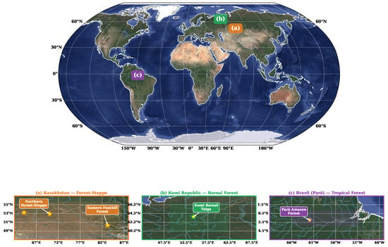
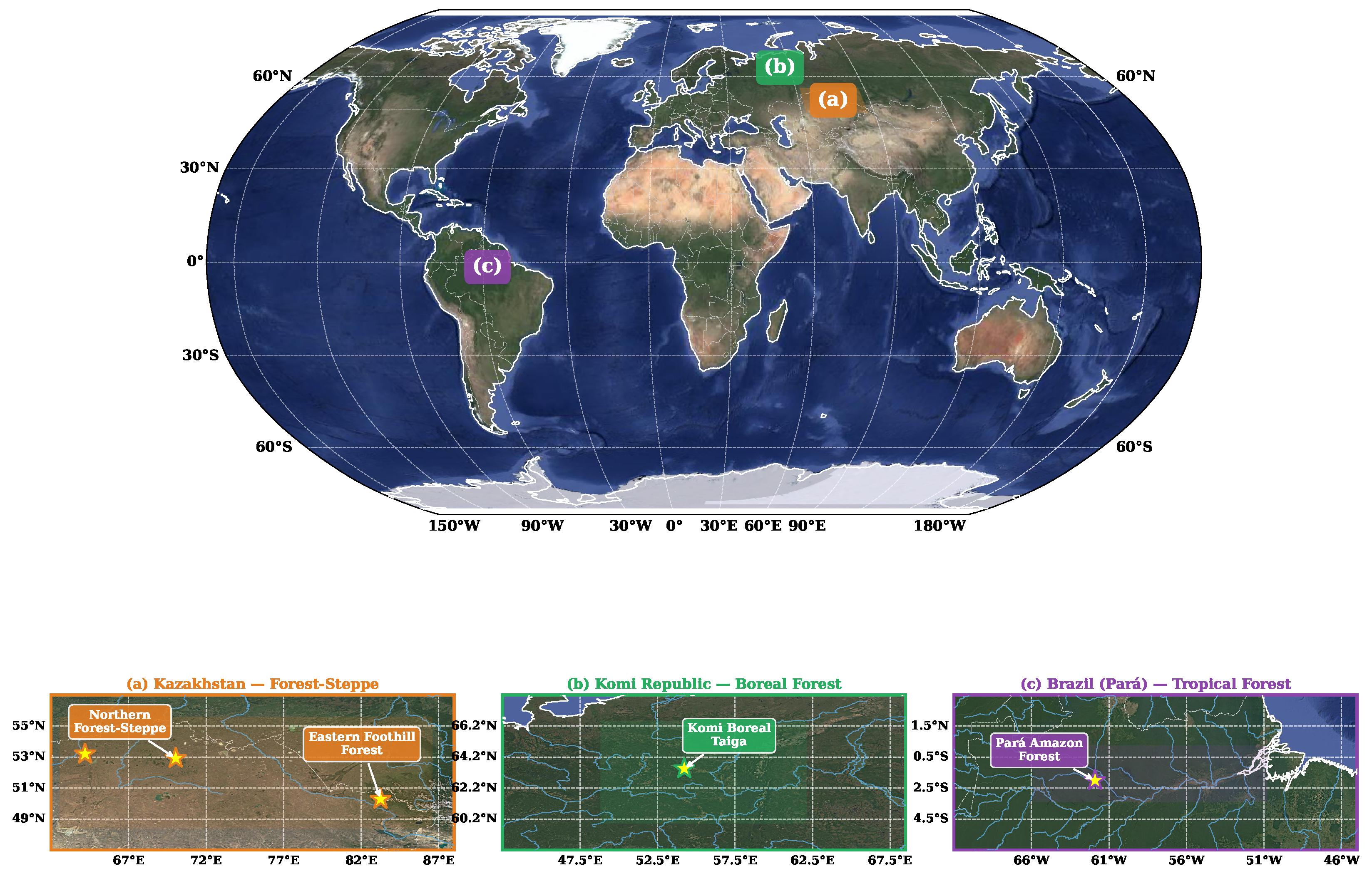
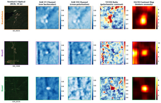
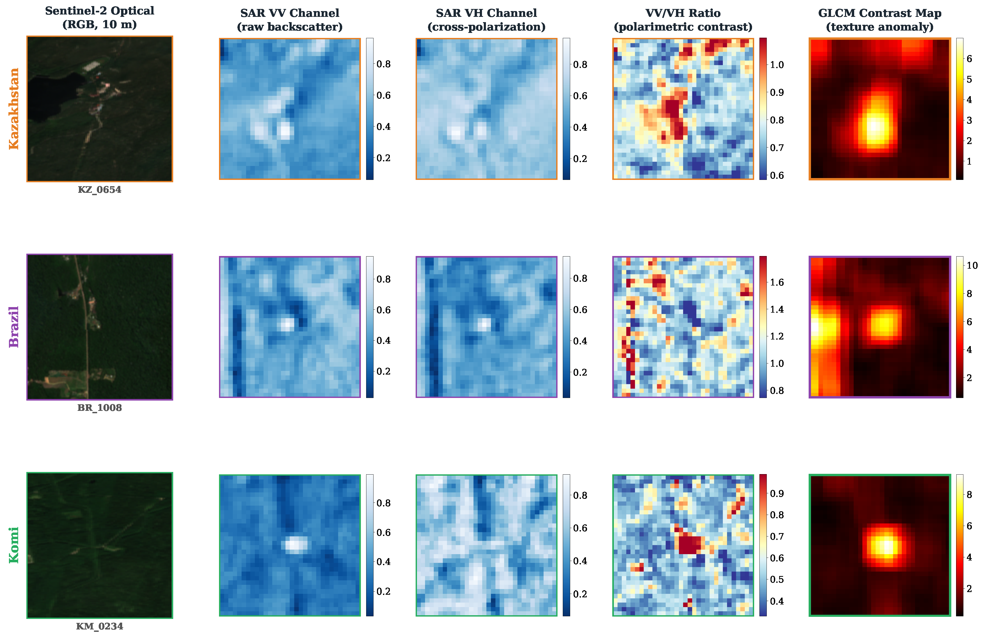
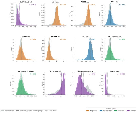
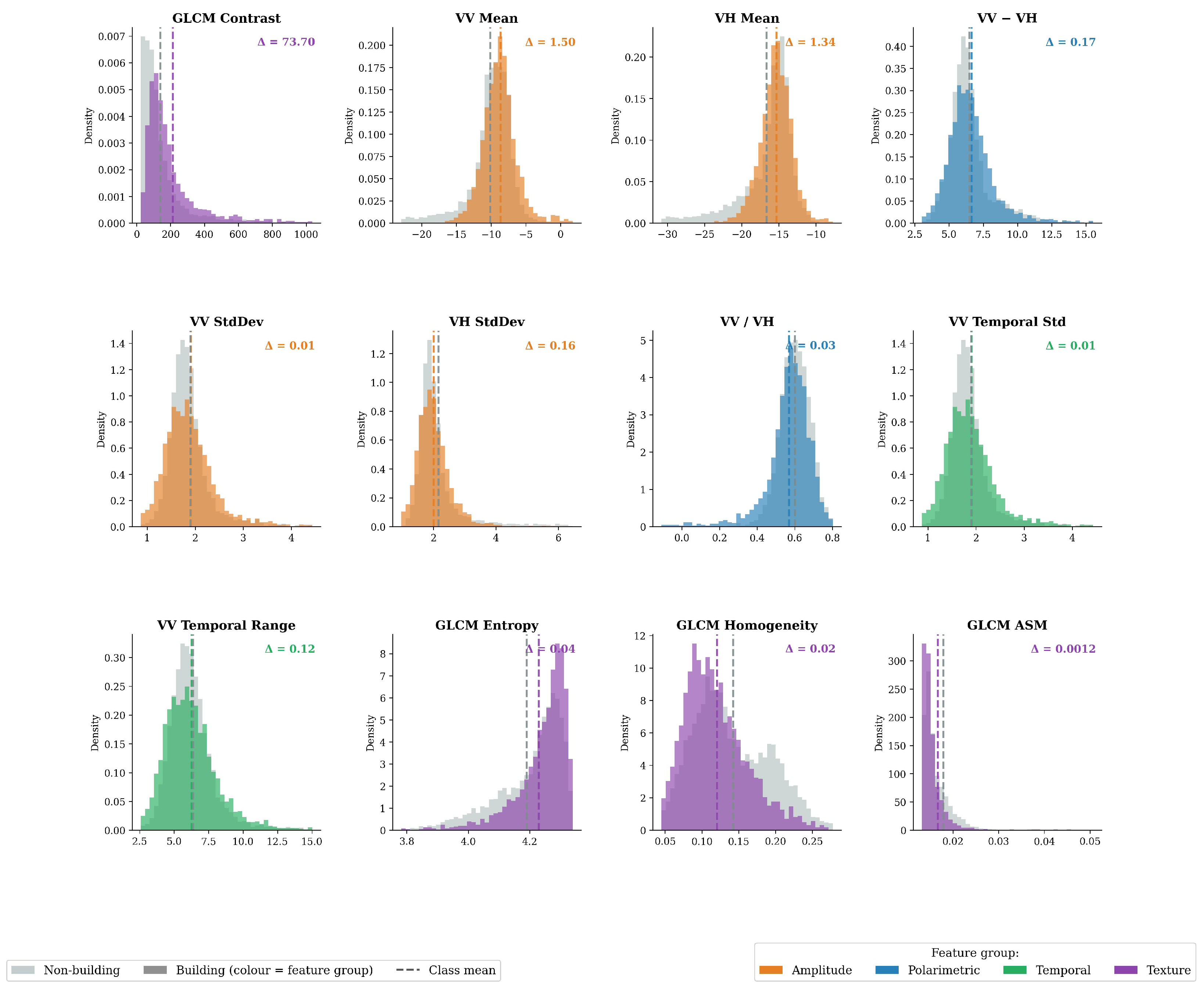
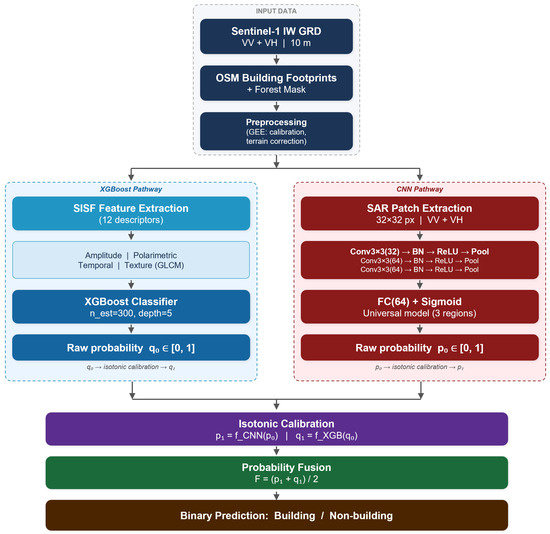
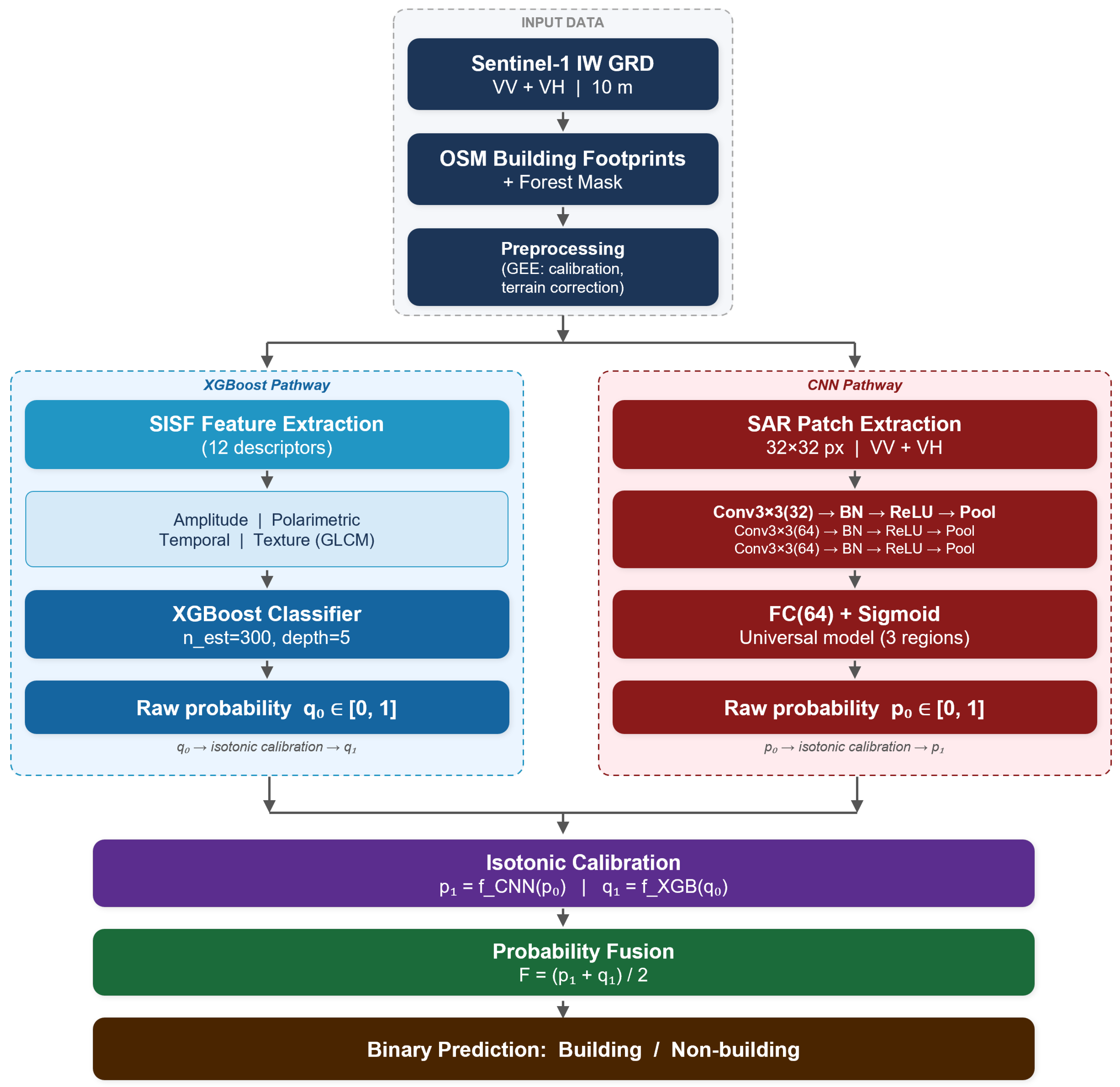
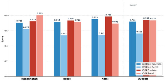
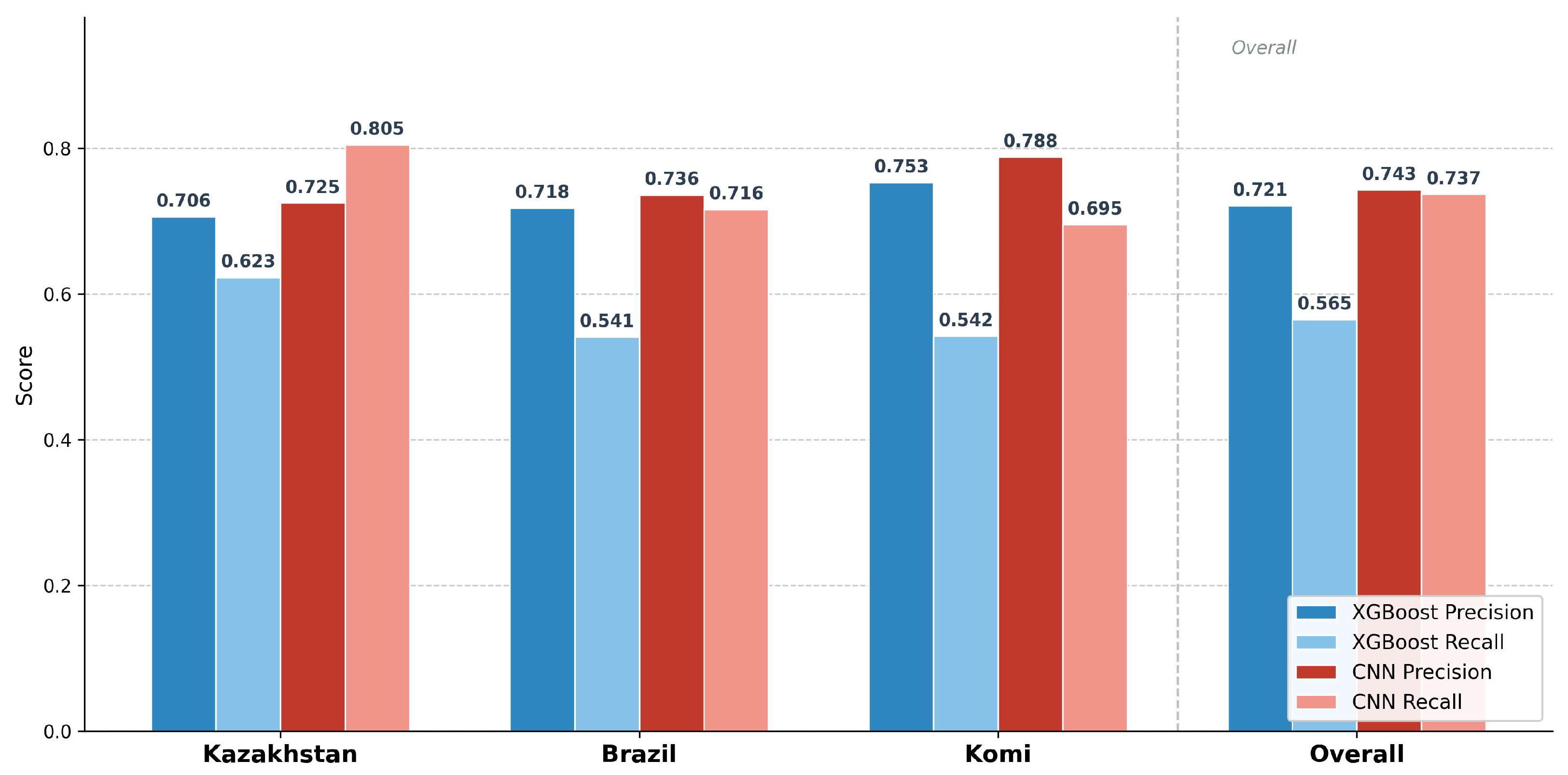
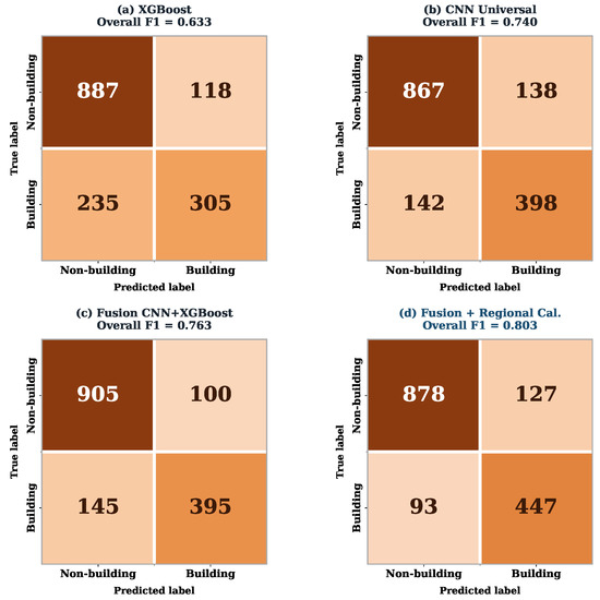
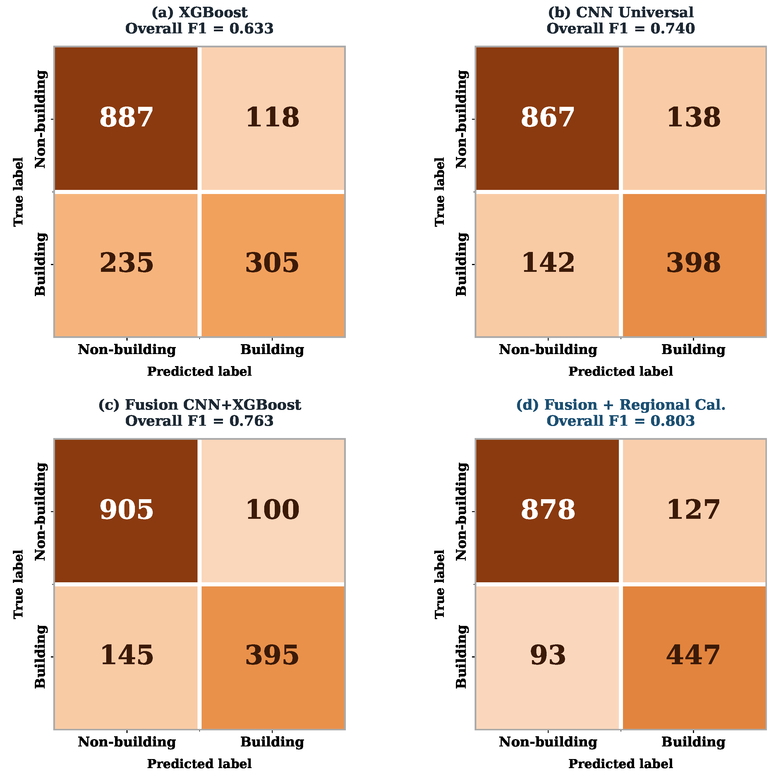
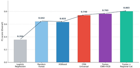
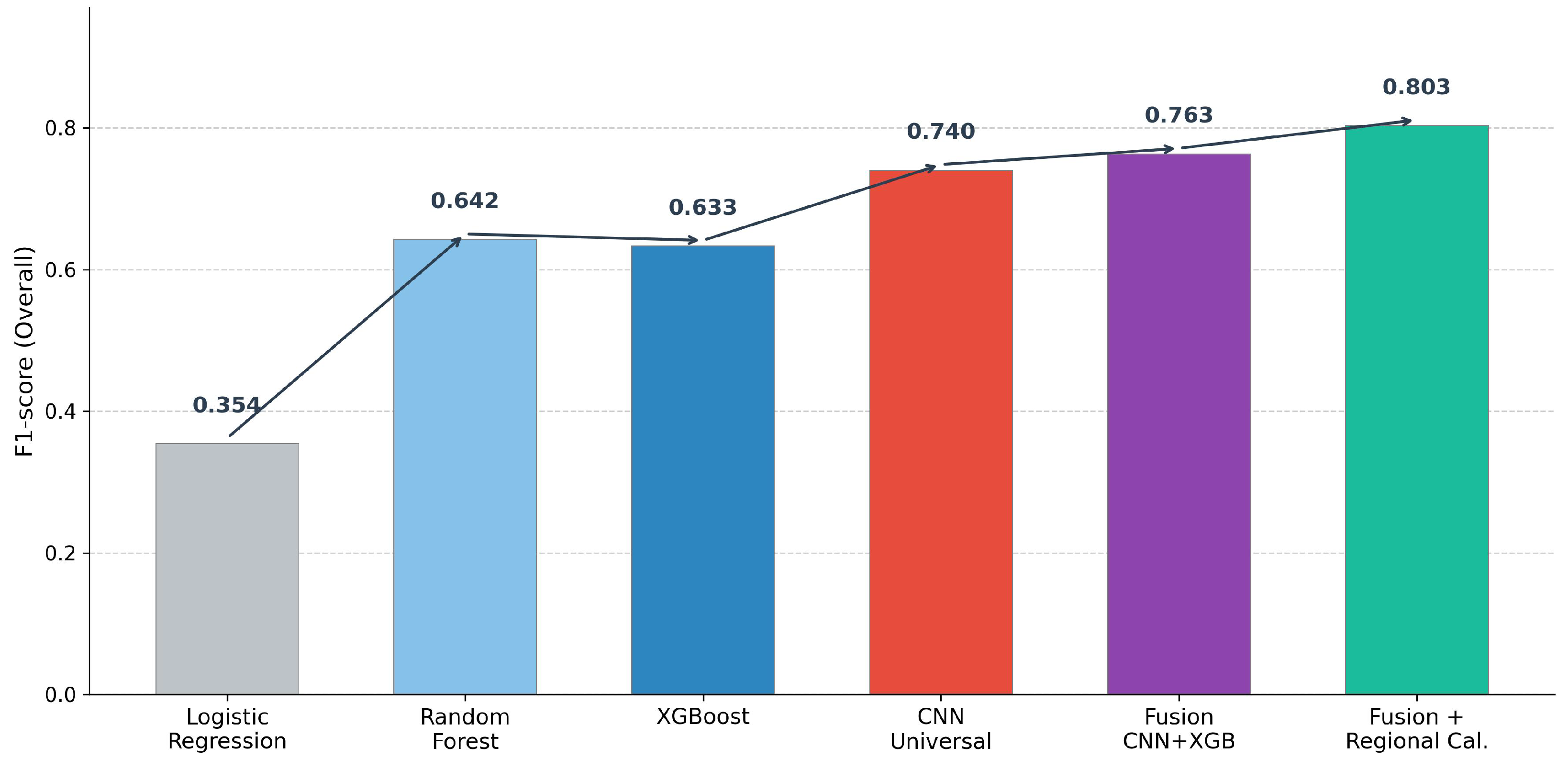
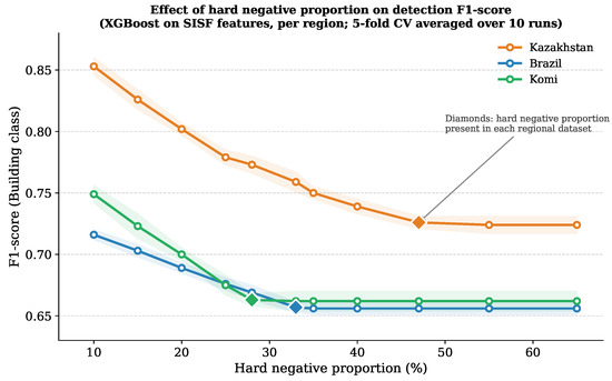
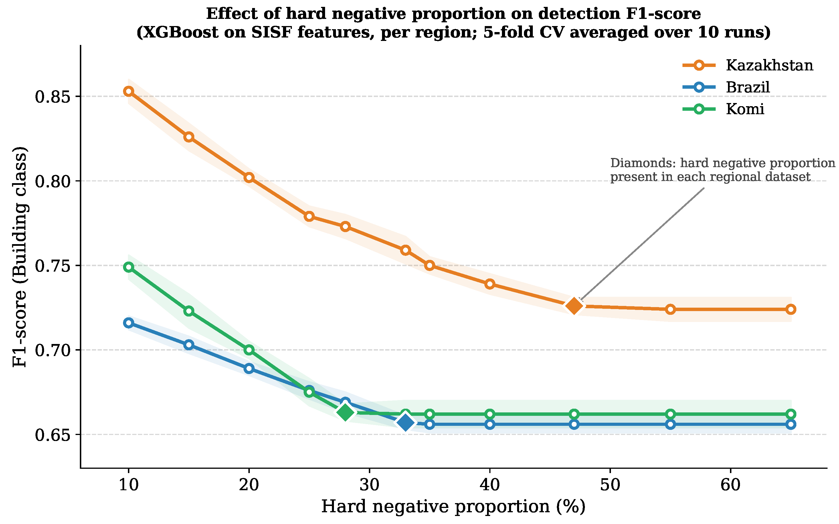
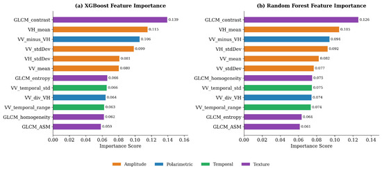
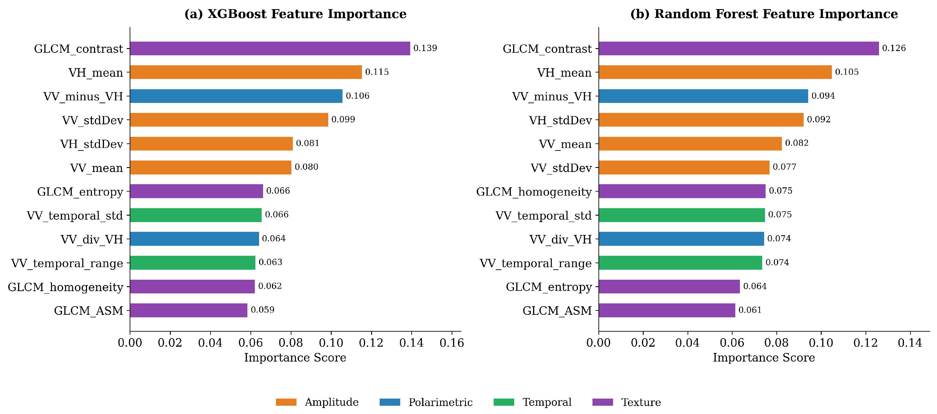
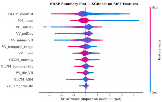
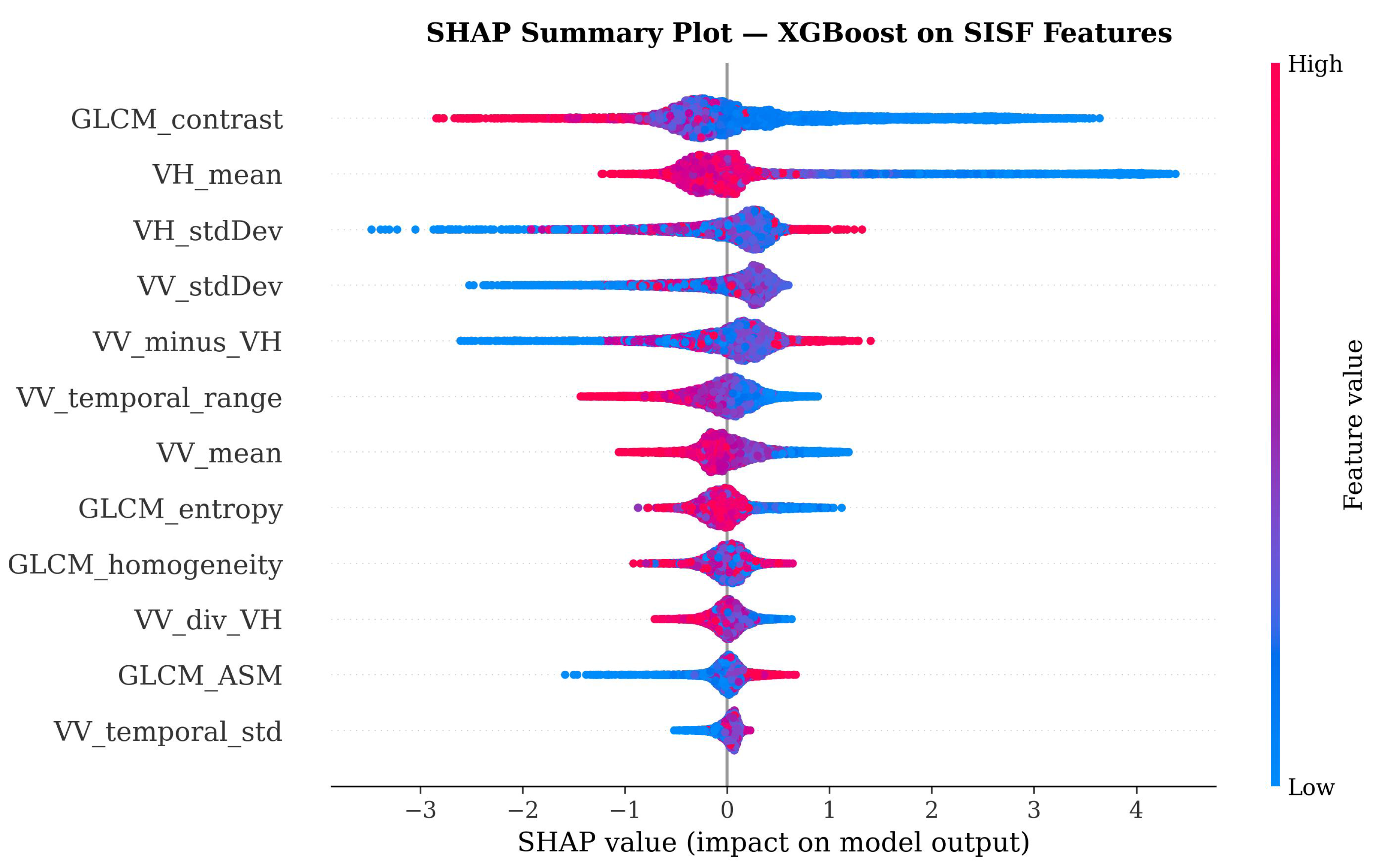
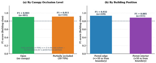
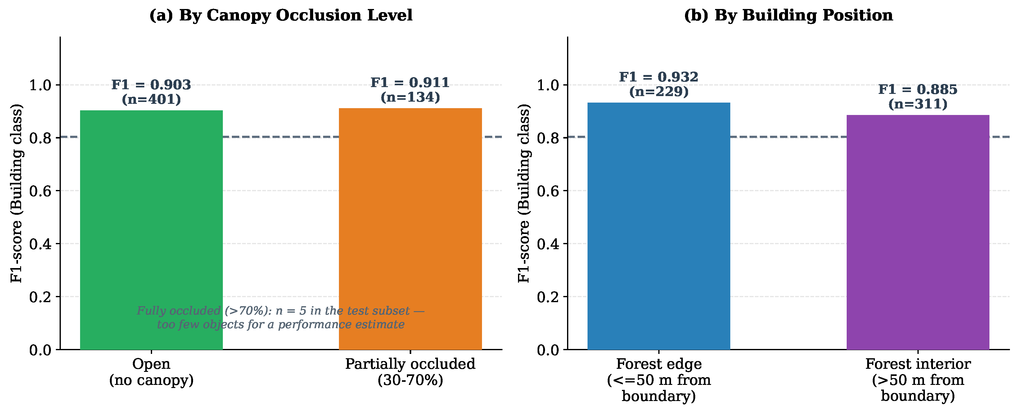
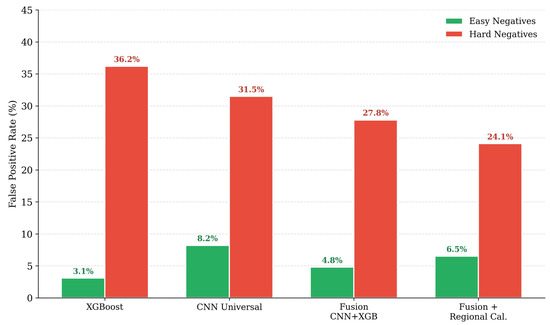
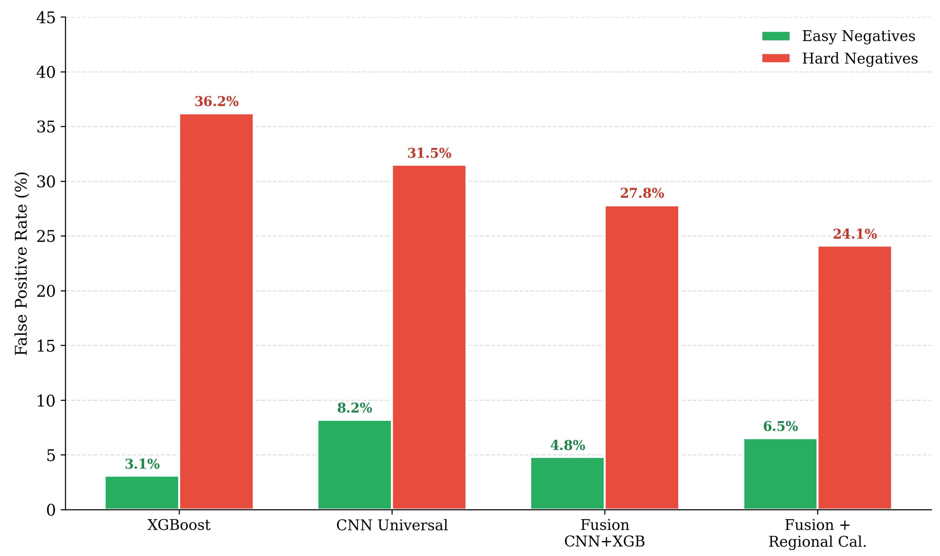

Disclaimer/Publisher’s Note: The statements, opinions and data contained in all publications are solely those of the individual author(s) and contributor(s) and not of MDPI and/or the editor(s). MDPI and/or the editor(s) disclaim responsibility for any injury to people or property resulting from any ideas, methods, instructions or products referred to in the content. |
© 2026 by the authors. Licensee MDPI, Basel, Switzerland. This article is an open access article distributed under the terms and conditions of the Creative Commons Attribution (CC BY) license.