Estimating Weather Effects on Well-Being and Mobility with Multi-Source Longitudinal Data

Abstract

Understanding the influence of weather on human well-being and mobility is essential to promoting healthier lifestyles. In this study we employ data collected from 151 participants over a continuous 30-day period in Switzerland to examine the effects of weather on well-being and mobility. Physiological data were retrieved through wearable devices, while mobility was automatically tracked through Google Location History, enabling detailed analysis of participants’ mobility behaviors. Mixed effects linear models were used to estimate the effects of temperature, precipitation, and sunshine duration on well-being and mobility while controlling for potential socio-demographic confounders. In this work, we demonstrate the feasibility of combining multi-source physiological and location data for environmental health research. Our results show small but significant effects of weather on several well-being outcomes (activity, sleep, and stress), while mobility was mostly affected by the level of precipitation. In line with previous research, our findings confirm that normal weather fluctuations exert significant but moderate effects on health-related behavior, highlighting the need to shift research focus toward extreme weather variations that lie beyond typical seasonal ranges. Given the potentially severe consequences of such extremes for public health and health-care systems, this shift will help identify more consistent effects, thereby informing targeted interventions and policy planning.

1. Introduction

Since the advent of the “theory of climates”, most famously articulated in “The Spirit of Laws” by Montesquieu [1], who argued that variations in climate shape people’s temperament, behavior, and even political institutions, scholars have long speculated on the influence that meteorological and seasonal dynamics exert on human well-being and behavior. While early theory posited relatively deterministic effects, empirical research over the past decades has yielded a far more nuanced and inconclusive picture. Systematic reviews indicate that meteorological influences are often moderate at best and context-specific [2,3]. This divergence reflects not only the complexity of human responses to environmental factors but also recurrent methodological and measurement limitations that constrain the reliability of prior findings.

Comparative assessments of systematic reviews have shown that work on temperature and weather effects frequently suffers from deficiencies in protocol registration, risk-of-bias assessment, and reporting transparency, raising questions about the robustness of previous conclusions [4]. Umbrella reviews further highlight that confidence in the existing evidence is often low to critically low, largely due to inconsistent operationalization of outcomes, high heterogeneity across studies, and limited ability to address confounders or interactions [5]. Meta-analyses on ambient temperature and mental health corroborate these findings, showing that although associations can be detected, effect sizes are highly variable, heterogeneity is substantial, and analytical approaches rarely capture lagged or non-linear effects [2].

Further complications arise when contrasting objective weather measurements with subjective perceptions of weather. Studies show only weak correspondence between meteorological indicators and self-reported experiences of weather, suggesting that perceptual and reporting biases may distort observed associations [6,7,8]. Similarly, subjective well-being measures, often collected through self-reported surveys or experience sampling, are prone to recall bias, mood effects, contextual influences, and missing responses, which can lead to inconsistencies between reported and actual states [9,10]. This gap is not trivial, as much of the existing evidence relies on self-reported well-being or retrospective survey data, meaning that discrepancies between experienced and measured conditions could systematically distort effect estimates. The issue is equally salient for mobility, since weather is known to influence transport choices, activity locations, and the use of active versus motorized modes. Yet research demonstrates that self-reported travel adaptations to weather often diverge from mobility patterns captured through GPS or sensor-based tracking, suggesting that individuals may underreport, misremember, or misclassify their behavioral responses to meteorological variation [11,12]. Capturing places visited, weather conditions, and objective well-being through multimodal, high-resolution tracking is, therefore, crucial to disentangling actual behavioral and affective changes from perceptual bias and to generating more credible estimates of the true impact of meteorological variability.

In light of these gaps, we contribute to the growing research on the impact of weather on well-being and mobility through the analysis of longitudinal objective and subjective multi-source data collected as part of an observational study conducted in Switzerland in 2024. Through the integration of weather data with high spatial and temporal resolution, systematic data filtering, and the use of mixed effects linear regression models, we estimate the effects of weather on several outcomes related to objective and subjective well-being and on distances traveled with different transportation types while controlling for potential socio-demographic confounders. Our work contributes to the field of environmental health research by demonstrating the feasibility of integrating objective multi-source data to derive practical insights into the effect of environmental factors on humans. Its design mitigates between-person confounding, ensures temporal granularity, and addresses measurement limitations, thereby offering a robust contribution to understanding whether—and to what extent—weather variations shape human well-being and behavioral choices.

The structure of the paper is as follows: Section 2 provides an overview of previous research investigating the relationships between weather, well-being, and mobility choices. Section 3 describes the study protocol, the data used, and the statistical methods that we employed. Section 4 reports the estimates of the weather effects on well-being and mobility that we drew from our sample of observations. Finally, Section 5 provides a critical discussion of the results and of their limitations, while Section 6 summarizes the work and provides insights for future works.

2. Related Work

The previous literature provides evidence that atmospheric weather has an effect on both well-being [13] and daily travel behaviors [14]. Among several well-being outcomes, researchers have investigated the relationship between weather and subjective well-being [15,16], happiness [17,18], sleep [19,20,21,22], physical activity and sedentary behaviors [23,24], and anxiety and depression [25]. However, results are often inconsistent across studies, with studies reporting small or non-significant effects [24]. As an example, Feddersen et al. found that warm and sunny days are associated with higher levels of self-reported well-being [16], while Connolly et al. reported that in regions with hot weather, an increase in temperature levels causes a decrease in well-being [15]. Weather effects on well-being during the COVID-19 pandemic were also analyzed, with results reporting no influence of weather on mental well-being during the pandemic [24]. The different results reported in the literature on the effects of weather may be due to different methodologies in the self-assessment of well-being, with studies involving large cohorts solely relying on self-reported information, which may be affected by recall bias and aggregation over long time windows [15,16,17,18,23,24,25]. Instead, few studies have focused on the use of objective data to measure the impact of weather on well-being. The use of objective measurements helps to reduce the risks of recall bias in self-reported data, and it also allows researchers to collect several measurements of well-being over extended periods of time with a smaller burden being put on study participants, as few to none active tasks are needed. The use of commercial devices for well-being tracking, such as smartwatches and smart rings, allows for the continuous and passive monitoring of physiological data through which objective indicators can then be derived and used for the estimation of weather effects on well-being. An example use of objective data in the sleep domain is from Mattingly et al. [19]. In this study, the authors employed a subset of the Tesserae dataset [26] to assess the impact of weather on sleep duration, bedtime, and wake-up times through a year-long multimodal study. The authors exploited objective data collected through smartwatches (Garmin Vivosmart 3) and linked them to the weather of participants’ homes. The results from this study (216 participants, 51,836 observations) indicated small but statistically significant seasonal and weather effects, with bedtimes and wake-up times being later with the increase in temperature values and sleep duration being lower with an increase in the length of the day. Recently, Li et al. [22] reported their analysis on more than 23 millions observations and more than 200 thousands participants, with the increase in temperature being linked to reduced total sleep time. In a study with an objective measure of physical activity through accelerometers (127 participants, 720 observations), Sumukadas et al. found day length, temperature, and sunshine to explain 73% of the variance in measured daily activity [27]. In a similar study by Feinglass et al., the authors analyzed the effects of weather on a three-year-long study with six weekly measurement waves (241 participants, 4823 observations) and found daylight hours, cold and hot days, and light or heavy rainfall to be associated with lower physical health [28]. Similar results on physical activity were found in several studies using accelerometer-based measurements or step counts from commercial wearables [23,29,30].

Well-being is not the only domain that has been investigated in relationship with weather data. A vast literature corpus deals with the analysis of the effects of atmospheric weather (temperature, precipitation, humidity, etc.) on human mobility and transportation mode choices [14]. Climate change, with its consequences on weather, can have significant impacts on human mobility and transportation choices; therefore, it is necessary to investigate how transport mode choices are influenced by weather to take appropriate actions in time [31]. Similar to what we previously described for well-being, in the mobility domain, authors have either relied on self-reported information through surveys [11,32,33,34] or based their analysis on objective data (e.g., GPS traces provided by smartphones or dedicated trackers, smart card transactions, etc.) [35,36,37,38,39]. Among studies that focused on the use of objective mobility data, Pang et al. built a global dataset based on mobility assessed through data retrieved via social networks and found nice weather (high temperature and moderate pressure) to have a positive impact on human mobility [35]. Lepage et al. integrated data from bike sharing, taxi, and public transport companies to analyze transportation demand under different meteorological conditions [38]. Otim et al. used a total of 2671 GPS trajectories from Beijing to analyze transport mode choices [39]. Even though several studies focusing on the assessment of the effects of weather on mobility make use of objective data, the majority of them are typically cross-sectional, with surveys containing information from each study participant only for a single day/trip, thus failing to capture intra-subject fluctuations due to weather differences.

3. Materials and Methods

3.1. Study Protocol

We recruited a total of N = 294 study participants for 30-day data collection as part of the project “RENEWAL—Tackling the energy and well-being impact of telework practices through multisource data”. We enrolled study participants from six companies and institutions located in Canton Ticino (Switzerland) on a rolling basis from February to May 2024. We requested participants to always wear a Garmin Vivosmart 5 (Garmin Ltd., Olathe, KA, USA) to track physiological data continuously, day and night. We employed Google Location History (GLH) (Google LLC, Mountain View, CA, USA) to track trips and locations using Google Takeout to retrieve mobility data. Self-reported information was also provided by participants in different formats. At the start of the study, they completed an onboarding questionnaire mainly focused on socio-demographic and work- and leisure-related information. Furthermore, they also filled out the Short-Form Health Questionnaire (SF-12), which provides a self-assessment of physical (PCS, physical component score) and mental health (MCS, mental component score) [40]. Throughout the study, participants received a daily diary asking to self-assess their sleep quality, health, and stress for the day, together with information about their workday, leisure activities, and transport mode choices.

Study participants were thoroughly informed about the study and signed an informed consent form before taking part in the study. The study protocol followed the Declaration of Helsinki for studies involving human participants [41] and was reviewed by the local ethical committee (SwissEthics Clarification of Responsibility Req-2023-0106).

3.2. Weather Data

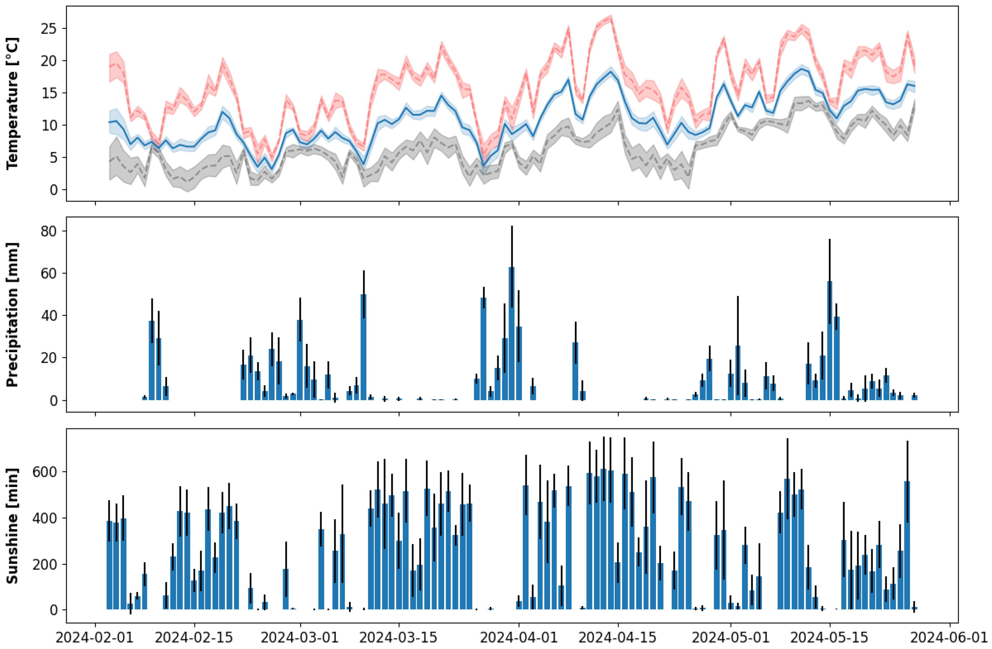
We employed MeteoSwiss (https://opendatadocs.meteoswiss.ch/, accessed on 7 September 2025) as a weather data source, using the closest weather station to the participants’ home as a daily source of weather information. A total of 7 weather stations (Acquarossa, Biasca, Cadenazzo, Cevio, Locarno, Lugano, and Stabio) were used for the retrieval of weather information, spanning the whole area of Canton Ticino where the study was conducted. MeteoSwiss provides several types of aggregated weather information for each station. Among them, there are average, maximum, and minimum air temperature at 5 cm and 2 m above ground; average wind speed; relative humidity; total precipitation during the day; and absolute and relative sunshine duration. We retrieved all these types of weather information and linked them to each participant by using the weather station closest to their home address. Figure 1 shows the variation in weather across all the available weather stations for the whole duration of the study for temperature, precipitation, and sunshine duration. Considering all the available measurements across the weather stations, median ($p_{25},p_{75}$) temperature at 2 m above ground was 10.5 (7.9, 13.6), with increasing temperatures from February (7.5, 6.0 to 9.0) to May (14.4, 12.8 to 15.9). For slightly more than half of the days (53%), the total daily precipitation was lower than 0.1 mm. For the remaining days it was lower than 30 mm (40%), with few exceptions with total daily precipitation greater than 30 mm (7%). March and April were the two months with the highest amount of recorded precipitations across all stations, with the highest being March. Finally, median ($p_{25},p_{75}$) sunshine duration was 191 (2, 413) min and, similarly to temperature, increased from February (131, 0 to 320) to April (324, 47 to 544), followed by a decrease in May (131, 11 to 340).

Figure 1. Temperature (top), precipitation (middle), and sunshine duration (bottom) data from the day of the first participant in up to the day of the last participant out. Temperature data are shown as mean (blue solid line), minimum (gray dashed line), and maximum (red dashed line), together with the corresponding 95% CIs. Precipitation and sunshine duration data are reported as means (bar height) and standard deviations (error bars). All data refer to the 7 weather stations that were employed for the retrieval of weather data.

3.3. Data Processing

Physiological data were retrieved through Garmin Health API (https://developer.garmin.com/gc-developer-program/health-api/, accessed on 7 September 2025). This free service provides, upon direct acceptance from study participants, several data points related to the physiological domain and computed through Garmin proprietary algorithms running on the smartwatch provided to the study participants [42]. We processed these data (heart rate, steps, sleep, etc.) to extract daily features across several domains related to well-being. Mobility data were instead retrieved from GLH services, which automatically extracts location visits and movements through GPS and network data on smartphones [43,44,45]. Google does not allow for the automatic retrieval of GLH data through API. Therefore, we instructed the study participants to export these data through Google Takeout and upload the resulting zip file in a dedicated section of the mobile application that was provided to them for the duration of the study. We then processed location data and extracted daily traveling distances according to different modes of transport: active mobility (cycling, running, and walking), motor vehicles (car, motorcycle, taxi, etc.), and public transport (bus, tram, and train).

3.4. Data Filtering

We filtered the collected data to consider only days with reliable data. Filtering was performed using different data sources. First, we considered only weekdays, excluding weekends, as they may be characterized by different patterns of activity, mobility, and sleep and may not be representative of typical behaviors [19,46]. Second, we considered only days in which the total time the Vivosmart 5 was worn was at least 70% (approximately 17 h out of 24), so that aggregated features of steps and stress were representative of the majority of the day. Daily wearing time was determined based on heart rate samples, with the assumption that heart rate values are provided only when the smartwatch is placed on the wrist. Then, we considered only those days for which night sleep was automatically tracked by the provided smartwatches, excluding nights with missing sleep data or with manual insertion of sleep times.

In addition to wearing time and sleep, we also accounted for the amount of daily coverage for location data. Daily coverage was computed by resampling the provided GLH location segments (i.e., a movement from point A to point B with a given transportation type) into location bins of 5 min, considering the participant as being in the same static location if the distance between the end of one location segment and the start of the following location segment was smaller than 200 m. This was performed with the aim of keeping only days for which participants’ locations and travel patterns were known for most of the day, thus justifying the usage of the closest weather station to their home to determine the weather data for each day. We chose to keep only days for which at least 70% of the location was known, using the same threshold that we set for the wearing time of the smartwatch. The use of location data allowed us also to identify travel days, represented by those days in which participants were traveling away from their home. Using this information, we excluded days for which the maximum reported distance from their home was equal to 300 km, suggesting that travels away from home for which weather data retrieved from the weather station closest to the home address did not represent a reliable source of weather information. This traveling threshold was chosen similar to [19], which chose to keep only observations with an average distance from home greater than 320 km. Finally, to further improve the reliability of our estimates employing longitudinal data, we additionally filtered our dataset to consider only study participants for which at least 10 observations were available.

3.5. Statistical Modeling

To examine the effects of weather on well-being and mobility, we used mixed effects linear regression (MELR) models. Since our dataset consists of repeated observations for each participant over time, this approach properly accounts for inter-individual variability [47]. The general specification for our MELR models is

$$y={\beta }_0+{\beta }_1·x_1+{\beta }_2·x_2+\cdots +{\beta }_n{x}_n+U_i+e$$

(1)

where y is the outcome of interest, ${\beta }_0$ is the intercept, ${\beta }_{1,\dots ,n}$ are the coefficients for predictors $x_{1,\dots ,n}$, $U_i$ is the random intercept assigned to the i-th participant, and e is the residual error.

We tested hierarchical models including increasing blocks of predictors. First, we built an empty model with no fixed effects (Model 1). Then, we integrated socio-demographic information collected at the baseline as time-invariant predictors for the model (Model 2). At this stage, we included the following time-invariant predictors: age, work organization, sex, having a supervisor role at work, having children, SF-12 Mental Component Score, and SF-12 Physical Component Score. The choice of these predictors was based on previous studies which included similar sets of measurements and predictors [19]. The supervisor role was derived based on the computation of the International Standard Classification of Occupations (ISCO), which was derived based on work-related information reported in the onboarding questionnaire. Participants with an ISCO code of “Managers” or “Technicians and Associate professionals” were defined as having a supervisor role. Finally, we added three weather predictors into a final model (Model 3): mean daily temperature, total daily precipitation, and daily sunshine duration. We used the closest weather station to the participants’ home to assign daily weather information. The choice of these three predictors (temperature, precipitation, and daily sunshine duration) was driven by the choices of (i) having the same set of predictors across both well-being and mobility domains and (ii) sharing a similar set of predictors with previous related works [19,24]. In our modeling we did not include wind speed, as we assumed it to have no effect on well-being-related outcomes [27]. During the monitoring period, no snow was measured and was thus excluded from the modeling.

The statistical modeling of the data was performed on Python 3.13 using the following libraries: pandas v2.2.3 [48], scipy 1.15.2 [49], and statsmodels v0.14.4 [50].

3.6. Outcomes

We focused our analysis on the effects of weather on 11 outcomes related to participant well-being and mobility, which are summarized in Table 1. For well-being, we examined seven health-related features across different physiological domains. In the activity domain, we considered the number of steps taken during the wake period as retrieved by the Garmin wearable (from wake-up to bedtime), as well as the percentage of time spent in sedentary behavior during the same time window. Sleep was also assessed through Garmin data, looking at bedtime, wake-up time, and total sleep duration, with weather information from a given day being used to predict outcomes on the following night. Stress was examined using three complementary indicators. The first was the self-reported stress level, collected through daily diaries by asking participants, “Today, do you feel stressed? Stress refers to a condition in which you feel tense, restless, nervous or anxious, or cannot sleep at night because you are agitated”. Answers to this question were recorded on a 5-point Likert scale from 1 (Not at all) to 5 (Extremely). Following Norman [51], this measure was modeled as continuous, albeit originally ordered categorical. The second indicator was the daily average Garmin stress score, which ranges from 0 (no stress) to 100 (extreme stress) and is derived from heart rate and heart rate variability (HRV) measurements [52]. Finally, we considered night recovery, computed as the normalized percentage change in “body battery” a Garmin proprietary metric estimating the body’s available energy, during nighttime sleep, which can be considered both a measure of sleep quality and an indicator of stress while sleeping, which could be linked to reduced resting capabilities. For the mobility domain, we analyzed the total daily distance traveled by participants, with transportation modes being automatically detected through GLH. Distances traveled by plane were excluded, as they represent travel away from home, and we focused instead on three categories: active mobility, motor vehicles, and public transport.

Table 1. Detailed description of the outcomes considered for the MELR analysis, together with their source and scale. A.U.: Arbitrary Unit.

Domain	Outcome	Source	Description	Scale	Unit
Well-being	Daily Steps	Garmin	Count of daily steps while awake	≥0	Steps
	Sedentary %		% of time in sedentary state while awake	0–100	%
	Bedtime		Bedtime on next night	0–24	Hours
	Wake-Up Time		Wake-up on next night	0–24	Hours
	Total Sleep Time		Total amount of sleep hours	≥0	Hours
	Night Recovery		Normalized change in body battery while sleeping	0–100	%
	Daily Stress		Mean measured physiological stress	0–100	A.U.
	Self-Reported Stress	Diary	Perceived stress during the day	0–5	A.U.
Mobility	Active Mobility	GLH	Total daily distance traveled based on active mobility	≥0	km
	Motor Vehicle		Total daily distance traveled with motor vehicles	≥0	km
	Public Transport		Total daily distance traveled with public transport	≥0	km

For each outcome, we computed the intra-class coefficient (ICC), defined as

$$ICC={\displaystyle \frac{{\tau }_{U_{0}i}^2}{{\tau }_{U_{0}i}^2+{\sigma }_e^2}}={\displaystyle \frac{\mathrm{BP}\mathrm{Variation}}{\mathrm{BP}\mathrm{Variation}+\mathrm{WP}\mathrm{Variation}}}$$

where ${\tau }_{U_0}^2$ is the variance of the estimated random intercepts of the MELR models, ${\sigma }_e^2$ is the variance of the within-person residuals, BP stands for between-person, and WP for within-person [47]. With ICC values ranging from a minimum of 0 up to a maximum of 1, we can determine whether all the variance in the data is longitudinal (i.e., due to within-person changes), which results in an ICC of 0, or if it is only cross-sectional (i.e., due to between-person differences), which instead results in an ICC of 1.

4. Results

4.1. Dataset

Our initial dataset was composed of 8820 observations from the whole set of 294 study participants. Upon filtering the dataset with the conditions detailed in Section 3.4, we were left with an analytical sample of 151 participants and 2120 observations. Table 2 reports a summary of the socio-demographics characteristics of the study participants of the analytical sample. The majority of the participants were male (98, 65%). Median age was 42 years old, with males being older than females. An unbalanced distribution was found for the organization for which participants were working, with a higher proportion for company 5 (59, 51%). Similar proportions were found for having children, with 57% of females and 54% of males reporting having at least one children. Overall, 34% of the included study participants had a supervisory role at work, with a higher proportion of males (39%) than females (25%). The mean (min, max) number of observations per participant was equal to 14 (10, 22).

Table 2. Socio-demographic information of the participants available for analysis after filtering the complete dataset.

	Sex		Overall (N = 151)
	F (N = 53)	M (N = 98)
Age	42 (32, 47)	47 (37, 47)	42 (37, 47)
SF-12 MCS	43.45 (37.90, 51.59)	49.61 (44.30, 55.18)	47.91 (41.80, 53.04)
SF-12 PCS	55.70 (53.60, 57.40)	55.04 (52.00, 56.17)	55.30 (52.28, 56.59)
Company
C1	3 (6%)	17 (17%)	20 (13%)
C2	3 (6%)	13 (13%)	16 (11%)
C3	11 (21%)	12 (12%)	23 (15%)
C4	7 (13%)	13 (13%)	20 (13%)
C5	23 (43%)	36 (37%)	59 (39%)
C6	6 (11%)	7 (7%)	13 (9%)
Supervisor role	13 (25%)	38 (39%)	51 (34%)
Having children	30 (57%)	53 (54%)	83 (55%)

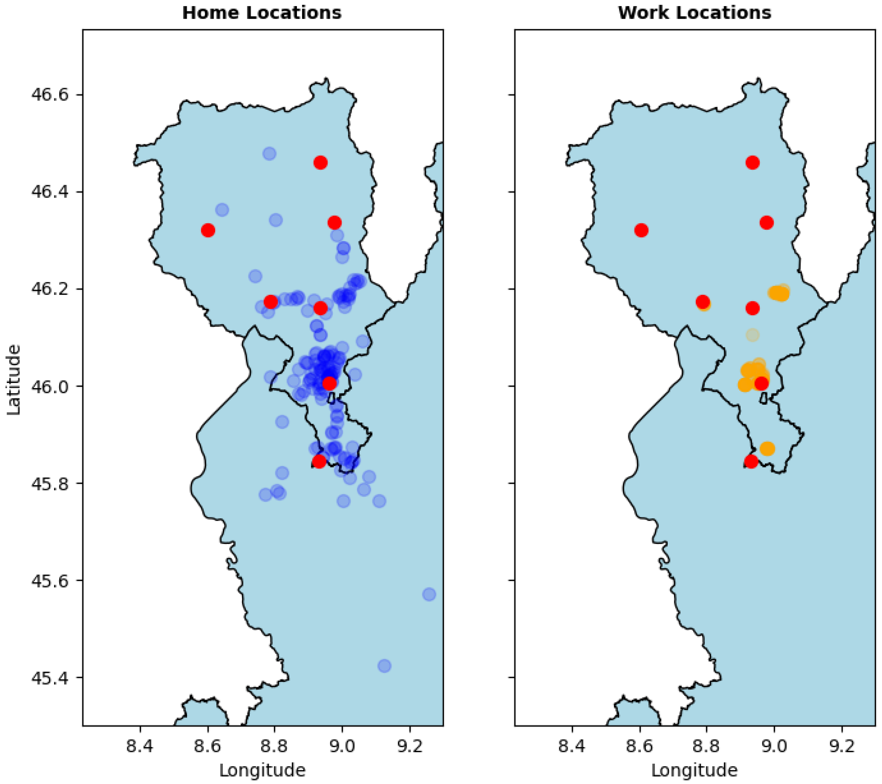
Figure 2 shows the coordinates of the seven weather stations, together with the location of both home and work addresses for the analytical sample. The median ($p_{25},p_{75}$) maximum daily distance between the self-reported home address and the closest weather station, used for linking weather data to participants’ daily measurements, was 8.9 (5.2, 18.8), with 95% of the available observations having a maximum daily distance from the closest weather station of 48.7 km. To assess the extent to which participants moved away from home while traveling, we also computed the maximum daily traveled distance from their home addresses, and we found a median ($p_{25},p_{75}$) distance of 7.6 km (2.8, 19.1). In the analytical sample, participants wore the smartwatch for a median ($p_{25},p_{75}$) percentage of time during their wake period of 100% (96.44, 100), with a median awake time of 16.75 h (15.92, 17.67). The location of the study participants during these days was tracked for a median ($p_{25},p_{75}$) number of daily hours equal to 24 (21.5, 24) using a threshold for the distance between two consecutive location segments of 200 m. The dataset covered 75 days starting from February up to May of the same year (2024), with an available number of observations per day across all study participants of 32 (2.5, 48).

Figure 2. Coordinates of weather stations employed for the retrieval of weather information (red dots) and home (left plot, blue dots) and work (right plot, orange dots) location coordinates of the subset of study participants used for the analysis.

Table 3 reports the descriptive statistics of the continuous variables (outcomes and weather) measured during the study across all study participants in the analytical sample over time. We also assessed the distribution of the weather changes experienced by them. For daily temperature, we computed the difference between the maximum and minimum daily mean temperature for each participant and found a median ($p_{25},p_{75}$) difference of 8.9 (7.8, 10.6) degrees. We performed the same analysis for sunshine duration, with a median ($p_{25},p_{75}$) difference between the maximum and minimum sunshine duration experience by participant of 10.7 (10.3, 11.8) daily hours. For daily precipitation, we counted the number of days in which the daily total precipitation was greater than 1 mm from midnight to midnight, resulting in a median ($p_{25},p_{75}$) number of days of 5 (4, 7) across analytical sample members.

Table 3. Descriptive statistics of the continuous variables. Bedtime and wake-up time are reported as hours from midnight.

		$\mathit{\mu }$	$\mathit{\sigma }$	${\mathit{p}}_{25}$	${\mathit{p}}_{50}$	${\mathit{p}}_{75}$
Outcome	Daily Steps	8392.07	3682.85	5782.25	7859.50	10,280.00
	Sedentary %	82.12	7.58	77.71	83.17	87.40
	Total Sleep Time [Hours]	7.14	1.35	6.35	7.17	7.98
	Bedtime [Hours]	−0.48	1.36	−1.40	−0.65	0.30
	Wake-Up Time [Hours]	6.95	1.31	6.15	6.83	7.52
	Mean Stress [%]	50.71	14.64	40.23	51.51	61.20
	Self-Reported Stress [1–5]	2.47	0.98	2.00	2.00	3.00
	Night Recovery [%]	58.37	27.57	34.74	57.90	83.20
	Active Mobility [km]	2.77	5.81	0.00	0.59	2.63
	Motor Vehicles [km]	31.32	49.92	0.35	16.69	41.39
	Public Transport [km]	8.99	30.86	0.00	0.00	1.85
Weather	Temperature [°C]	11.20	3.17	8.80	11.20	13.00
	Precipitation [mm]	5.56	11.85	0.00	0.00	3.80
	Sunshine [Hours]	5.25	4.16	0.34	5.27	9.12

4.2. Weather Effects on Well-Being

4.2.1. Activity

Table 4 and Table 5 report the results of the MELR modeling of daily steps and the percentage of time in sedentary state, respectively. The ICC value for daily steps was 0.378, indicating that around 40% of the variance in the measurements is due to within-person changes over time, with the remaining variance due to between-person differences. We did not find any significant effect of weather features (temperature, precipitation, and sunshine duration) on the number of steps per day. Both in Model 2 and in Model 3, the mental and physical components of the health assessment carried out at baseline were positively associated with the number of steps per day, with people in better health status (higher MCS/PCS) walking more during the day. Interestingly, one organization (C5) was characterized by a significant positive coefficient, further justifying the inclusion of the company predictor in the modeling.

Table 4. Results of Model 1, Model 2, and Model 3 predicting the total number of daily steps while awake. For the sake of clarity, coefficients are rounded to the nearest integer. Significant coefficients are highlighted in bold. *: $p<0.05$; **: $p<0.01$; ***: $p<0.001$.

	Daily Steps
	Model 1		Model 2		Model 3
	Coef.	CI	Coef.	CI	Coef.	CI
Intercept	8470 ***	8086 to 8854	8011 ***	6607 to 9416	7538 ***	6052.0 to 9024.0
Age			5	−38 to 48	6	−37 to 49
Sex [0 = female]			−439	−1251 to 373	−432	−1242 to 379
Company [0 = C1]
C2			−367	−1856 to 1121	−448	−1936 to 1039
C3			925	−467 to 2317	851	−539 to 2241
C4			728	−681 to 2136	546	−871 to 1964
C5			1422 *	190.0 to 2654	1256 *	16 to 2495
C6			755	−865 to 2374	742	−875 to 2359
Supervisor role [0 = No]			−113	−927 to 702	−118	−932 to 695
Having children [0 = No]			−80	−861 to 701	−81	−860 to 698
SF-12 MCS			66 **	19 to 112	66 **	20 to 113
SF-12 PCS			86 **	22 to 150	87 **	23 to 151
Temperature					41	−13 to 95
Precipitation					−7	−19 to 6
Sunshine duration					30	−9 to 70
Marginal R2	0.000		0.062		0.067
ICC	0.378

Table 5. Results of Model 1, Model 2, and Model 3 predicting the percentage of sedentary time while awake. Significant coefficients are highlighted in bold. *: $p<0.05$; **: $p<0.01$; ***: $p<0.001$.

	Sedentary %
	Model 1		Model 2		Model 3
	Coef.	CI	Coef.	CI	Coef.	CI
Intercept	81.989 ***	81.117 to 82.861	83.995 ***	80.842 to 87.149	85.487 ***	82.202 to 88.772
Age			0.021	−0.075 to 0.117	0.018	−0.078 to 0.115
Sex [0 = female]			2.31 *	0.488 to 4.132	2.295 *	0.475 to 4.114
Company [0 = C1]
C2			−1.014	−4.354 to 2.326	−0.798	−4.137 to 2.54
C3			−2.980	−6.107 to 0.146	−2.817	−5.940 to 0.306
C4			−1.940	−5.103 to 1.223	−1.489	−4.666 to 1.688
C5			−3.839 **	−6.605 to −1.073	−3.414 *	−6.193 to −0.636
C6			−3.472	−7.109 to 0.165	−3.456	−7.089 to 0.176
Supervisor role [0 = No]			−0.148	−1.977 to 1.681	−0.141	−1.967 to 1.686
Having children [0 = No]			−1.484	−3.235 to 0.267	−1.482	−3.231 to 0.266
SF-12 MCS			−0.063	−0.167 to 0.042	−0.064	−0.169 to 0.040
SF-12 PCS			−0.196 **	−0.340 to −0.053	−0.201 **	−0.345 to −0.057
Temperature					−0.115 *	−0.218 to −0.012
Precipitation					0.003	−0.021 to 0.026
Sunshine duration					−0.093 *	−0.168 to −0.017
Marginal R2	0.000		0.087		0.094
ICC	0.475

The additional activity-related outcome that we considered was the percentage of time spent in sedentary behavior during the day. For this outcome, we found an ICC value of 0.475, suggesting that with respect to daily steps, higher variance can be explained by within-person changes over time. We found a statistically significant effect of physical health, as assessed by the SF-12 PCS (Model 2: −0.195, 95% CI: −0.340 to −0.053, $p<0.01$; Model 3: −0.201, 95% CI: −0.345 to −0.057, $p<0.01$). For weather features, we found an increase temperature (−0.115, 95% CI: −0.218 to −0.012, $p<0.05$) as well as an increase in sunshine duration (−0.093, 95% CI: −0.168 to −0.017, $p<0.05$) to reduce the percentage of time spent in sedentary behavior, while no effect was found for the level of precipitation during the day.

4.2.2. Sleep

For the sleep domain, Table 6, Table 7 and Table 8 report the MELR coefficients resulting from the modeling of next-night total sleep time, next-night bedtime, and next-day wake-up time, respectively. Total sleep time is measured in decimal hours, while bedtime and wake-up time are reported as hours from midnight. The three sleep time measurements of total sleep time, bedtime, and wake-up time resulted in ICC values of 0.24, 0.42, and 0.35, respectively. These values suggest that variance in bedtime values is characterized by higher between-person differences, while for total sleep time, variance is more explained by within-person changes on a day-to-day level.

Table 6. Results of Model 1, Model 2, and Model 3 predicting total sleep time. Total sleep time is measured in decimal hours. Significant coefficients are highlighted in bold. **: $p<0.01$; ***: $p<0.001$.

	Total Sleep Time
	Model 1		Model 2		Model 3
	Coef.	CI	Coef.	CI	Coef.	CI
Intercept	7.147 ***	7.03 to 7.264	7.331 ***	6.899 to 7.763	7.025 ***	6.550 to 7.500
Age			−0.009	−0.022 to 0.005	−0.008	−0.021 to 0.005
Sex [0 = female]			−0.403 **	−0.653 to −0.152	−0.398 **	−0.648 to −0.148
Company
C2			0.002	−0.456 to 0.461	−0.038	−0.498 to 0.421
C3			0.173	−0.255 to 0.601	0.163	−0.264 to 0.591
C4			−0.086	−0.519 to 0.348	−0.177	−0.616 to 0.262
C5			0.109	−0.269 to 0.488	0.027	−0.357 to 0.410
C6			0.187	−0.311 to 0.686	0.194	−0.303 to 0.692
Supervisor role [0 = No]			−0.074	−0.325 to 0.177	−0.069	−0.320 to 0.181
Having children [0 = No]			0.052	−0.189 to 0.293	0.050	−0.191 to 0.290
SF-12 MCS			0.001	−0.013 to 0.016	0.001	−0.013 to 0.016
SF-12 PCS			−0.004	−0.024 to 0.015	−0.004	−0.024 to 0.016
Temperature					0.030 **	0.008 to 0.051
Precipitation					0.003	−0.002 to 0.008
Sunshine duration					0.000	−0.016 to 0.016
Marginal R2	0.000		0.036		0.039
ICC	0.240

Table 7. Results of Model 1, Model 2, and Model 3 predicting bedtime. Bedtime is measured in decimal hours from midnight. Significant coefficients are highlighted in bold. *: $p<0.05$; **: $p<0.01$; ***: $p<0.001$.

	Bedtime
	Model 1		Model 2		Model 3
	Coef.	CI	Coef.	CI	Coef.	CI
Intercept	−0.481 ***	−0.628 to −0.334	−0.871 **	−1.389 to −0.353	−1.018 ***	−1.566 to −0.470
Age			−0.017 *	−0.033 to −0.001	−0.016 *	−0.032 to −0.000
Sex [0 = female]			0.508 **	0.208 to 0.808	0.511 **	0.211 to 0.811
Company
C2			−0.271	−0.82 to 0.279	−0.292	−0.842 to 0.258
C3			0.045	−0.469 to 0.559	0.044	−0.470 to 0.558
C4			0.434	−0.086 to 0.954	0.384	−0.140 to 0.909
C5			0.321	−0.134 to 0.775	0.277	−0.181 to 0.736
C6			0.134	−0.464 to 0.732	0.139	−0.459 to 0.737
Supervisor role [0 = No]			0.099	−0.201 to 0.4	0.103	−0.198 to 0.404
Having children [0 = No]			−0.265	−0.553 to 0.024	−0.266	−0.555 to 0.022
SF-12 MCS			−0.005	−0.023 to 0.012	−0.005	−0.023 to 0.012
SF-12 PCS			−0.017	−0.041 to 0.007	−0.017	−0.040 to 0.007
Temperature					0.017	−0.003 to 0.036
Precipitation					0.002	−0.003 to 0.006
Sunshine duration					−0.005	−0.020 to 0.009
Marginal R2	0.000		0.093		0.094
ICC	0.415

Table 8. Results of Model 1, Model 2, and Model 3 predicting wake-up time. Wake-up time is measured in decimal hours from midnight. Significant coefficients are highlighted in bold. *: $p<0.05$; **: $p<0.01$; ***: $p<0.001$.

	Wakeup
	Model 1		Model 2		Model 3
	Coef.	CI	Coef.	CI	Coef.	CI
Intercept	6.959 ***	6.827 to 7.092	6.816 ***	6.357 to 7.275	6.326 ***	5.832 to 6.819
Age			−0.022 **	−0.036 to −0.008	−0.021 **	−0.035 to −0.007
Sex [0 = female]			0.089	−0.177 to 0.355	0.097	−0.169 to 0.364
Company
C2			−0.242	−0.729 to 0.245	−0.308	−0.796 to 0.181
C3			0.196	−0.259 to 0.651	0.184	−0.272 to 0.64
C4			0.269	−0.191 to 0.73	0.121	−0.345 to 0.587
C5			0.374	−0.029 to 0.776	0.241	−0.166 to 0.648
C6			0.292	−0.237 to 0.822	0.306	−0.225 to 0.836
Supervisor role [0 = No]			−0.012	−0.278 to 0.255	−0.003	−0.27 to 0.264
Having children [0 = No]			−0.22	−0.476 to 0.035	−0.225	−0.481 to 0.031
SF-12 MCS			−0.007	−0.023 to 0.008	−0.007	−0.023 to 0.008
SF-12 PCS			−0.019	−0.04 to 0.002	−0.019	−0.04 to 0.002
Temperature					0.049 ***	0.029 to 0.069
Precipitation					0.006 *	0.001 to 0.01
Sunshine duration					−0.004	−0.019 to 0.01
Marginal R2	0.000		0.09		0.10
ICC	0.347

The results of our modeling of total sleep time show a small significant effect of daily mean temperature on total sleep time (95% CI: 0.6 to 3.0, $p<0.01$), with an average 1.8 min increase per one-degree increase in daily mean temperature. Except for sex, no socio-demographic predictor was found to be significantly associated with total sleep time. In our results, we found that males slept, on average, 24.2 min less than females (Model 2: 95% CI: −39.2 to −9.1, $p<0.01$; Model 3: 95% CI: −38.9 to −8.9, $p<0.01$).

The effect of daily temperature that we found for total sleep time disappeared for bedtime (Table 7), for which only socio-demographic factors (age and sex) were found to be significantly associated with sleep onset time. In particular, older participants and females tended to go to bed earlier, with bedtime decreasing by about 1 min for each additional year of age (Model 2 95% CI: −2.0 to −0.06, $p<0.05$; weather model 95% CI: −1.9 to 0, $p<0.05$). Females, compared with males, went to bed about 30 min earlier (Model 2: −30.5 min, 95% CI −48.5 to −12.5, $p<0.01$; Model 3: −30.7 min, 95% CI −48.7 to −12.7, $p<0.01$).

Moving onto the modeling of wake-up time (Table 8), we found a significant positive coefficient of temperature (2.9, 95% CI: 1.7 to 4.1, $p<0.001$), and a smaller but still significant positive effect of the level of daily precipitation on the wake-up time (0.4, 95% CI: 0.06 to 0.6, $p<0.05$). These results suggest that the increase in total sleep time due to higher temperatures can be explained with a delay in wake-up time, rather than an anticipation of bedtime. Similar to bedtime, we found a negative association between age and wake-up time, with older people waking up 1.3 min earlier for each unit increase in age (Model 2: 95% CI: −2.2 to 0.0, $p<0.01$; weather model 95% CI: −2.1 to 0.0, $p<0.01$).

4.2.3. Stress and Recovery

Table 9, Table 10 and Table 11 report the MELR coefficients resulting from the modeling of mean stress during the day, self-reported stress level, and next-night recovery, respectively. The stress values were those characterized by the highest ICC value, equal to 0.66, with the variance being mostly explained by differences between people in the mean stress value. Instead, self-reported stress and night recovery were both characterized by an ICC of 0.37. For the mean stress during the day assessed through physiological data, we found that an increase in mean daily temperature and sunshine duration led to increased levels of measured stress during the day (daily temperature: 0.176, 95% CI: 0.016 to 0.336, $p<0.05$; sunshine duration: 0.143, 95% CI 0.027 to 0.260, $p<0.05$). Among the socio-demographic predictors, only the SF-12 MCS was statistically significant (Model 2: −0.341, 95% CI: −0.582 to −0.104, $p<0.01$; Model 3: −0.341, 95% CI: −0.581 to −0.101, $p<0.01$), with people having higher mental health scores experiencing less stress during the day.

Table 9. Results of Model 1, Model 2, and Model 3 predicting mean stress value during the day. Mean stress goes from a minimum of 0 (no stress) to a maximum of 100 (high stress). Significant coefficients are highlighted in bold. *: $p<0.05$; **: $p<0.01$; ***: $p<0.001$.

	Mean Stress
	Model 1		Model 2		Model 3
	Coef.	CI	Coef.	CI	Coef.	CI
Intercept	50.878 ***	48.94 to 52.815	47.498 ***	40.271 to 54.725	45.177 ***	37.788 to 52.566
Age			−0.016	−0.237 to 0.204	−0.012	−0.234 to 0.209
Sex [0 = female]			−1.07	−5.242 to 3.101	−1.047	−5.229 to 3.134
Company
C2			3.934	−3.715 to 11.582	3.602	−4.067 to 11.271
C3			4.003	−3.167 to 11.173	3.76	−3.428 to 10.948
C4			5.925	−1.326 to 13.176	5.242	−2.046 to 12.53
C5			4.359	−1.982 to 10.700	3.714	−2.658 to 10.087
C6			7.442	−0.895 to 15.780	7.422	−0.935 to 15.779
Supervisor role [0 = No]			−0.588	−4.779 to 3.604	−0.598	−4.799 to 3.604
Having children [0 = No]			0.139	−3.868 to 4.146	0.136	−3.880 to 4.153
SF-12 MCS			−0.343 **	−0.582 to −0.104	−0.341 **	−0.581 to −0.101
SF-12 PCS			0.196	−0.133 to 0.525	0.203	−0.127 to 0.533
Temperature					0.176 *	0.016 to 0.336
Precipitation					−0.001	−0.038 to 0.036
Sunshine duration					0.143 *	0.027 to 0.260
Marginal R2	0.000		0.076		0.080
ICC	0.659

Table 10. Results of Model 1, Model 2, and Model 3 predicting the self-reported stress value. Self-reported stress goes from a minimum of 1 (no stress) to a maximum of 5 (extreme stress). Significant coefficients are highlighted in bold. *: $p<0.05$; ***: $p<0.001$.

	Self-Reported Stress
	Model 1		Model 2		Model 3
	Coef.	CI	Coef.	CI	Coef.	CI
Intercept	2.487 ***	2.385 to 2.588	2.350 ***	2.004 to 2.696	2.64 ***	2.272 to 3.008
Age			0.002	−0.009 to 0.012	0.001	−0.010 to 0.011
Sex [0 = female]			0.244 *	0.044 to 0.444	0.238 *	0.040 to 0.437
Company
C2			−0.04	−0.407 to 0.326	−0.000	−0.365 to 0.364
C3			0.258	−0.085 to 0.601	0.266	−0.075 to 0.606
C4			0.224	−0.123 to 0.571	0.316	−0.032 to 0.664
C5			0.035	−0.269 to 0.338	0.117	−0.187 to 0.421
C6			0.142	−0.257 to 0.541	0.134	−0.262 to 0.53
Supervisor role [0 = No]			−0.031	−0.232 to 0.17	−0.036	−0.236 to 0.163
Having children [0 = No]			−0.187	−0.38 to 0.005	−0.184	−0.375 to 0.007
SF-12 MCS			−0.038 ***	−0.049 to −0.026	−0.038 ***	−0.049 to −0.027
SF-12 PCS			−0.010	−0.026 to 0.006	−0.010	−0.026 to 0.006
Temperature					−0.030 ***	−0.045 to −0.016
Precipitation					−0.003	−0.006 to 0.000
Sunshine duration					0.004	−0.006 to 0.015
Marginal R2	0.000		0.107		0.114
ICC	0.370

Table 11. Results of Model 1, Model 2, and Model 3 predicting night recovery. Night recovery is measured as percentage from 0 (no recovery) to 100 (maximum recovery). Significant coefficients are highlighted in bold. *: $p<0.05$; ***: $p<0.001$.

	Night Recovery
	Model 1		Model 2		Model 3
	Coef.	CI	Coef.	CI	Coef.	CI
Intercept	58.277 ***	55.438 to 61.117	56.490 ***	45.6 to 67.379	58.948 ***	47.438 to 70.459
Age			−0.163	−0.497 to 0.17	−0.166	−0.500 to 0.167
Sex [0 = female]			4.482	−1.813 to 10.777	4.479	−1.825 to 10.783
Company
C2			2.459	−9.081 to 13.998	2.797	−8.771 to 14.364
C3			3.754	−7.04 to 14.548	4.139	−6.674 to 14.951
C4			0.894	−10.027 to 11.816	1.523	−9.497 to 12.544
C5			−0.579	−10.13 to 8.971	0.056	−9.578 to 9.691
C6			0.727	−11.833 to 13.286	0.810	−11.767 to 13.386
Supervisor role [0 = No]			1.535	−4.781 to 7.85	1.587	−4.738 to 7.912
Having children [0 = No]			−4.411	−10.463 to 1.641	−4.425	−10.485 to 1.635
SF-12 MCS			0.194	−0.167 to 0.555	0.190	−0.172 to 0.552
SF-12 PCS			−0.048	−0.546 to 0.449	−0.059	−0.557 to 0.439
Temperature					−0.125	−0.531 to 0.281
Precipitation					0.015	−0.078 to 0.109
Sunshine Duration					−0.301 *	−0.597 to −0.004
Marginal R2	0.000		0.024		0.027
ICC	0.373

The modeling of self-reported stress values showed similar results for socio-demographics, with an increase in mental health status leading to lower daily self-reported values (Model 2: −0.038, 95% CI: −0.049 to −0.026, $p<0.001$; Model 3: −0.038, 95% CI: −0.049 to −0.027, $p<0.001$). However, opposite results were found for the effects of weather, with higher temperatures being related to lower self-reported stress values (−0.03, 95% CI: −0.045 to −0.016, $p<0.001$).

Finally, no socio-demographic characteristic was found to be a significant predictor of night recovery as measured through the Garmin body battery feature (Table 11). Among the weather variables, only sunshine duration was significant, with higher sunshine duration leading to lower recovery values (−0.30, 95% CI: −0.597 to −0.004, $p<0.05$).

4.3. Weather Effects on Mobility

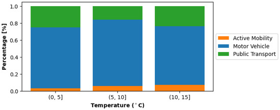
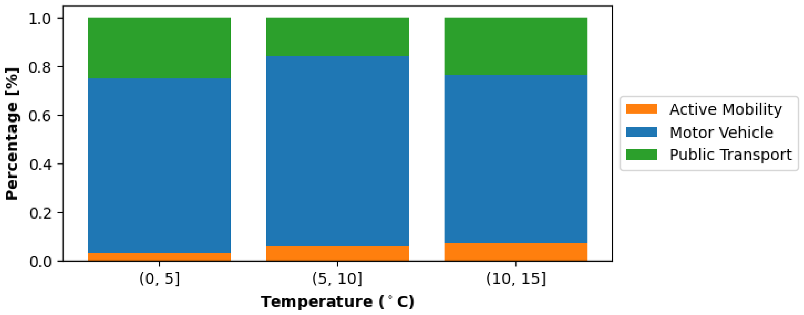
After examining the effects of weather on well-being, we turned to mobility behaviors and patterns. Figure 3 shows the percentage of distance travelled with different mobility types with respect to ranges of mean daily temperature across the analytical sample. Table 12, Table 13 and Table 14 present the results of the MELR models predicting daily distance traveled based on active mobility, motor vehicles, and public transportation, respectively. For all three modes, most of the variance in daily distance was attributable to within-person fluctuations over time, as indicated by ICC values of 0.26 for active mobility, 0.17 for motor vehicles, and 0.12 for public transportation.

Figure 3. Percentage of daily distance traveled with the three different mobility types (active mobility, motor vehicles, and public transport) with varying mean daily temperatures.

Table 12. Results of Model 1, Model 2, and Model 3 predicting daily kilometers based on active mobility (cycling, running, and walking). Significant coefficients are highlighted in bold. *: $p<0.05$; ***: $p<0.001$.

	Active Mobility Distance [km]
	Model 1		Model 2		Model 3
	Coef.	CI	Coef.	CI	Coef.	CI
Intercept	2.774 ***	2.255 to 3.292	1.766	−0.097 to 3.629	1.38	−0.651 to 3.412
Age			0.103 ***	0.046 to 0.161	0.104 ***	0.047 to 0.161
Sex [0 = female]			1.131 *	0.052 to 2.21	1.139 *	0.065 to 2.213
Company [0 = C1]
C2			−0.203	−2.180 to 1.775	−0.293	−2.264 to 1.679
C3			0.715	−1.130 to 2.560	0.579	−1.258 to 2.416
C4			−0.808	−2.675 to 1.060	−1.015	−2.898 to 0.869
C5			1.648 *	0.015 to 3.281	1.457	−0.189 to 3.104
C6			−0.800	−2.948 to 1.348	−0.841	−2.979 to 1.296
Supervisor role [0 = No]			−0.305	−1.386 to 0.775	−0.327	−1.403 to 0.748
Having children [0 = No]			−0.308	−1.347 to 0.730	−0.306	−1.339 to 0.727
SF-12 MCS			0.030	−0.032 to 0.092	0.030	−0.032 to 0.092
SF-12 PCS			0.008	−0.078 to 0.093	0.010	−0.075 to 0.095
Temperature					0.029	−0.063 to 0.120
Precipitation					−0.022 *	−0.043 to −0.001
Sunshine duration					0.062	−0.005 to 0.129
Marginal R2	0.000		0.053		0.061
ICC	0.264

Table 13. Results of Model 1, Model 2, and Model 3 predicting daily kilometers in motor vehicles (car, motorcycle, and taxi). Significant coefficients are highlighted in bold. **: $p<0.01$; ***: $p<0.001$.

	Motor Vehicle Distance [km]
	Model 1		Model 2		Model 3
	Coef.	CI	Coef.	CI	Coef.	CI
Intercept	30.729 ***	26.893 to 34.564	49.26 ***	36.082 to 62.438	43.307 ***	28.016 to 58.597
Age			0.08	−0.327 to 0.486	0.091	−0.319 to 0.501
Sex [0 = female]			3.536	−4.117 to 11.189	3.672	−4.048 to 11.392
Company [0 = C1]
C2			−27.850 ***	−41.872 to -13.827	−28.948 ***	−43.132 to −14.763
C3			−33.537 ***	−46.564 to -20.509	−34.438 ***	−47.592 to −21.284
C4			−29.332 ***	−42.536 to −16.127	−31.988 ***	−45.597 to −18.380
C5			−26.410 ***	−37.956 to −14.863	−28.794 ***	−40.688 to −16.900
C6			−22.570 **	−37.760 to −7.380	−22.722 **	−38.045 to −7.400
Supervisor role [0 = No]			6.952	−0.691 to 14.595	6.907	−0.803 to 14.618
Having children [0 = No]			1.634	−5.742 to 9.010	1.592	−5.847 to 9.030
SF-12 MCS			−0.104	−0.544 to 0.336	−0.104	−0.548 to 0.340
SF-12 PCS			0.200	−0.407 to 0.807	0.214	−0.398 to 0.826
Temperature					0.628	−0.205 to 1.461
Precipitation					−0.112	−0.306 to 0.081
Sunshine duration					0.194	−0.420 to 0.807
Marginal R2	0.000		0.059		0.062
ICC	0.172

Table 14. Results of Model 1, Model 2, and Model 3 predicting daily kilometers in public transportation (bus, train, and tram). Significant coefficients are highlighted in bold. *: $p<0.05$; **: $p<0.01$; ***: $p<0.001$.

	Public Transport Distance [km]
	Model 1		Model 2		Model 3
	Coef.	CI	Coef.	CI	Coef.	CI
Intercept	9.144 ***	7.028 to 11.26	3.300	−4.914 to 11.513	3.149	−6.301 to 12.598
Age			0.172	−0.081 to 0.426	0.171	−0.081 to 0.423
Sex [0 = female]			1.533	−3.238 to 6.303	1.441	−3.310 to 6.193
Company [0 = C1]
C2			4.707	−4.034 to 13.448	4.992	−3.738 to 13.722
C3			4.267	−3.853 to 12.387	4.578	−3.514 to 12.67
C4			5.637	−2.594 to 13.868	6.596	−1.783 to 14.974
C5			12.430 **	5.233 to 19.627	13.173 ***	5.853 to 20.494
C6			0.376	−9.092 to 9.843	0.47	−8.957 to 9.896
Supervisor role [0 = No]			−0.447	−5.212 to 4.317	−0.422	−5.166 to 4.322
Having children [0 = No]			−2.993	−7.591 to 1.605	−2.963	−7.541 to 1.615
SF-12 MCS			0.064	−0.211 to 0.338	0.069	−0.204 to 0.343
SF-12 PCS			−0.706 ***	−1.085 to −0.328	−0.703 ***	−1.079 to −0.326
Temperature					−0.178	−0.700 to 0.344
Precipitation					0.123 *	0.002 to 0.244
Sunshine duration					0.191	−0.194 to 0.575
Marginal R2	0.000		0.042		0.044
ICC	0.124

For active mobility (cycling, running, and walking), the complete model, Model 3, revealed significant effects of age, sex, and precipitation. Specifically, older individuals and men covered longer daily distances with active mobility, as indicated by positive associations with age (0.104, 95% CI 0.047 to 0.161, $p<0.001$) and sex (1.139, 95% CI: 0.065 to 2.213, $p<0.05$).

We observed a negative association between precipitation and active mobility (−0.022, 95% CI: −0.043 to −0.001, $p<0.05$), indicating that greater rainfall corresponded to shorter distances covered on foot or by bike. For daily distance traveled with motor vehicles, the model did not reveal any statistically significant effects of weather. Among the socio-demographic factors, only the employing organization showed an association with motor vehicle use, while no other predictors were significant.

Finally, for public transportation, Model 3 identified significant effects of both SF-12 PCS and precipitation. Better physical health (i.e., higher SF-12 PCSs) was associated with shorter distances traveled by public transport (−0.703, 95% CI −1.079 to −0.326, $p<0.001$), whereas higher precipitation levels corresponded to greater reliance on this mode of travel (0.123, 95% CI: 0.002 to 0.244, $p<0.05$).

5. Discussion

In this manuscript we reported the study design, methodology, and results obtained when assessing the impact of weather, as measured by mean daily temperature, level of precipitation, and sunshine duration, on ten different outcomes related to well-being (activity, recovery, sleep, and stress) and mobility. For our analysis, we used the dataset collected as part of the RENEWAL study, which involved a total of 294 participants for 30 continuous days and for which objective data (i.e., physiological data through Garmin Health API) and self-reported data (i.e., surveys and ecological momentary assessments) were retrieved. Given the longitudinal nature of our dataset, we employed MELR models to analyze how three key weather predictors, namely, mean daily temperature, total daily precipitation, and total sunshine duration, affect these outcomes, taking into account both intra-person and inter-person differences. To improve the robustness of our analysis, we filtered our daily observations with strict criteria to keep only reliable observations. We considered only weekdays in which the provided smartwatch was worn more than 70% of the time and for which automatic sleep tracking was available. Furthermore, we kept only days with at least 70% coverage in terms of location data, and we excluded days with presumed travels too far away from home (i.e., with maximum daily distance greater than 300 km), similar to what was performed in [19]. Our final dataset consisted of 2120 daily observations from 151 participants, spanning the period from February to May 2024, with a median ($p_{25},p_{75}$) number of observations available per participant of 14 (10, 22).

Our analysis showed modest effects of weather on both well-being and mobility outcomes. For well-being, MELR models found a positive effect of temperature on total sleep time, wake-up time, and physiological stress, while a negative association with temperature was found for self-reported stress values and the percentage of sedentary time during the day. The amount of sunshine during the day positively affected the physiologically measured stress and the percentage of sedentary time during the day, while negatively impacting recovery during the next-night sleep. We did not find any statistically significant association between weather and bedtime and the total number of daily steps. Our results for wake-up time are in line with what was found by Mattingly et al. [19] with objective sleep data tracked with Garmin smartwatches. The authors found a modest effect of daily temperature on wake-up time. However, their study was conducted over a longer period of time, with participants enrolled for approximately a year. Therefore, the authors were able to include seasonality among the predictors for the MELR models, and seasons resulted significant in the prediction of other sleep-related outcomes (total sleep time, bedtime, and wake-up time). In the same study, in contrast to our results, temperature was not found to be associated with total sleep time, which was instead affected by season, with sleep duration decreasing in spring with respect to winter. Similarly, in a recent paper by Li et al. [22], which included automatic sleep tracking through Huawei smartwatches, the authors found total sleep time to be reduced by approximately 10 min for every 10° increase in temperature. These contrasting results on sleep-related outcomes may be explained by the limited observation period of our study, with the majority of observations belonging to spring and with small temperature variations. Due to this, we were not able to include seasonality effects in our models, and we instead found weather to impact total sleep time and wake-up time, with findings suggesting a shift in wake-up times with the increase in temperature and bedtime remaining unaffected. As far as the activity domain is concerned, our results are in line with previous findings that reported increasing physical activity with the increase in temperature and sunshine duration [23,27,28,30]. Our models showed a statistically significant effect of temperature and sunshine duration on the percentage of time spent in active or highly active states (i.e., non-sedentary behavior) but not on the number of daily steps, suggesting an increase in the extent of physical activities not necessarily including walking or running exercises. Interesting, we found opposite results when assessing the impact of weather on stress. In our models, we used two different stress measurements: an objective stress measure, defined as the mean stress value reported by the Garmin smartwatch (i.e., a Garmin proprietary algorithm based on HRV and heart rate analysis [52]) and the self-reported stress value in the daily diaries. While we found warmer days to reduce the self-reported stress value, in line with previous large-scale survey-based studies [16,24], our analysis showed temperature and sunshine duration to increase the amount of physiological stress as measured through HRV and heart rate, which, to the best of our knowledge, is still unexplored in the available literature.

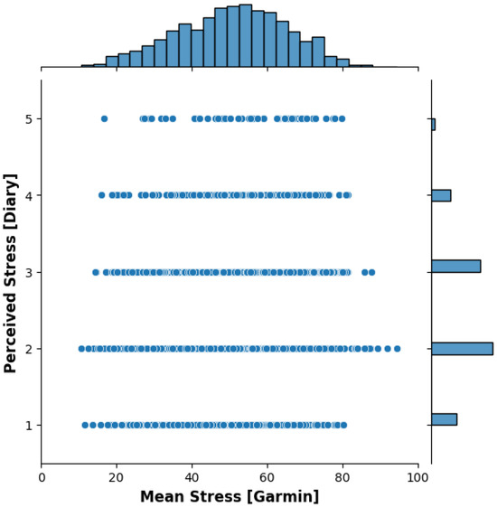
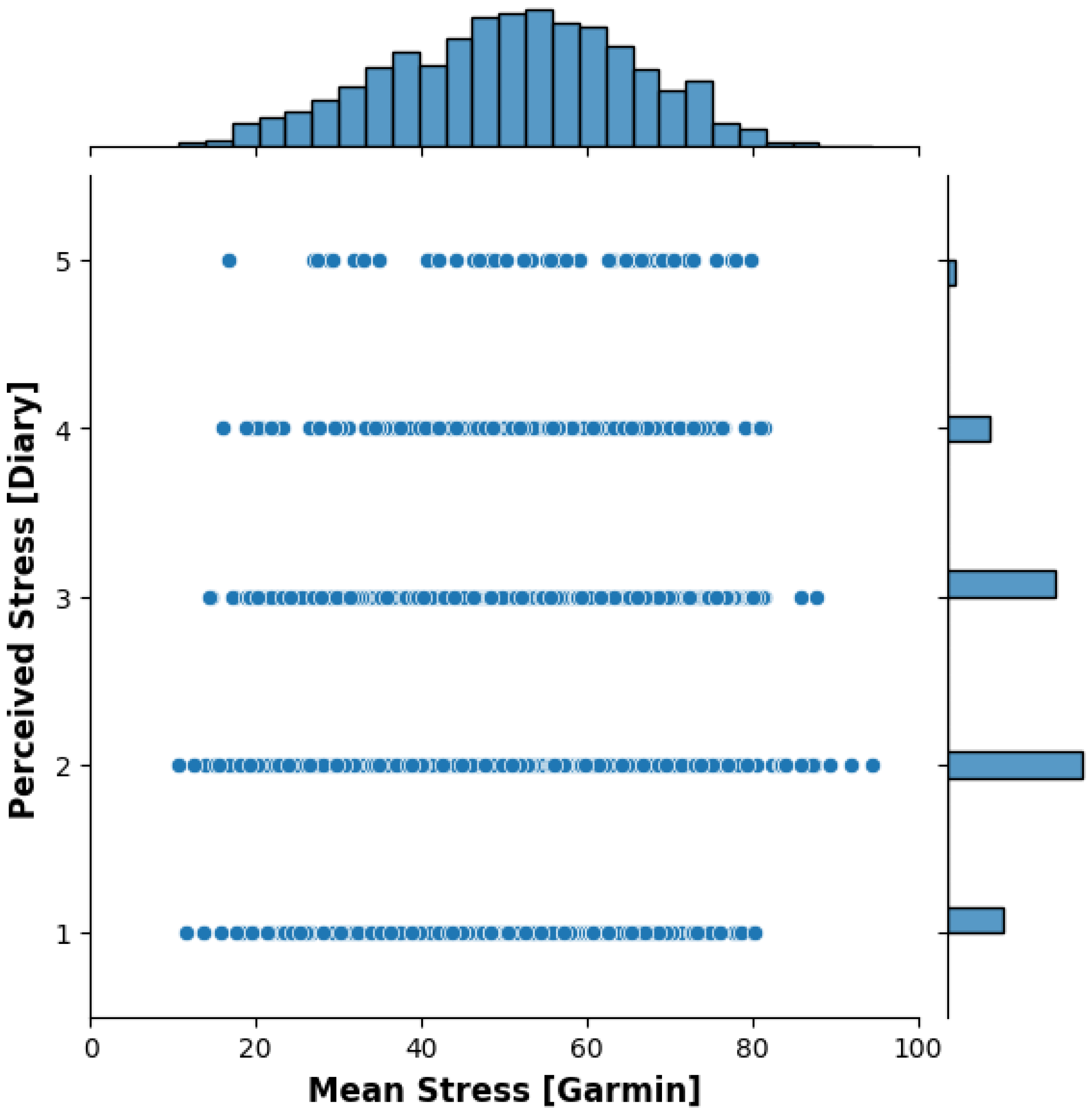
This can be explained by the fact that self-reported and physiological stress are two different representations, with authors finding small-to-medium effect sizes between self-reported stress and objective physiological stress measures [53]. We computed the repeated measure correlation between the two metrics [54], and we found a weak correlation of 0.07 ($p<0.01$). Figure 4 shows the joint plot of the two measurements, further highlighting differences between the two stress assessments. It is worth noting that self-reported stress values could also be affected by recall bias, especially when employing daily stress assessments and not ecological momentary assessments. Furthermore, objective stress measured by Garmin through their proprietary algorithms also takes into account the extent of activity and the recovery phases following it, thus suggesting that warmer and longer days are linked to a greater amount of activity carried out during the day, as confirmed by our results on effects of weather on sedentary behaviors. Finally, for well-being, we also assessed the impact of weather on night recovery, i.e., on the amount of “energy” recovered by the body while sleeping and being in a rest state. Our models showed a significant modest and negative effect of sunshine duration on this outcome.

Figure 4. Joint plot of Garmin mean stress during the wake period and self-reported perceived stress values in the daily diaries. Garmin stress values are continuous on a scale from 0 to 100, while self-reported stress was assessed with a 5-point Likert scale.

Moving on to the mobility domain, we assessed the impact of weather on the total daily traveled distance according to three different mobility types: active mobility, motor vehicles, and public transport. We found a statistically significant effect of precipitation on both active mobility and public transport, with a reduced distance traveled based on active mobility with the increase in precipitation, while the opposite holds for public transport, with increased distances with higher precipitation values. When modeling the distance traveled by motor vehicles, we did not find any significant effect of weather. This analysis may suggest an overall stability of distances traveled with motor vehicles, while distance traveled using active mobility transportation types (mainly walking or cycling) are replaced with public transportation in case of higher precipitations during the day. When compared with other studies using objective mobility and location data, Pang et al. found a positive effect of weather on overall mobility, without differentiating among different types of mobility [35]. Lepage et al. found precipitation to reduce the amount of bike sharing (i.e., indirect measurement of distance traveled based on active mobility) [38], while Otim et al. did not include precipitation among the predictors for transport mode choices and found higher temperature to increase the amount of the walking share and to reduce bike sharing [39].

This study does not come without limitations. First of all, when compared with other studies using objective data for well-being and mobility assessments, our dataset is smaller. In the two largest studies assessing the impact of weather on sleep, Mattingly et al. had a total of 51,836 observations [19] and Li et al. 23 million observations [22], which are way larger than our 2120 observations. These datasets also span multiple monitoring months, enabling to also assess the effect of seasons rather than only daily weather measurements. Ours, instead, was limited to a short observation period of four spring months during the year 2024, limiting the possibility of studying seasonal effects on the chosen outcomes. In addition to this, our observations were confined in the region of Canton Ticino (Switzerland) and northern Italy, and study participants were mostly office workers, male, and belonging to a single organization, thus limiting the generalization capabilities of our results, since other populations (e.g., shift workers) and/or countries with different weather conditions may experience different effects of weather on their well-being and mobility. Furthermore, while, on one hand, the strict filtering process that we carried out on the dataset left us with a reliable set of observations, on the other hand, it may have introduced a bias in the dataset, as only highly compliant participants were left in the analytical sample used for the modeling. In the filtering process, we excluded travel days with a maximum distance of 300 km away from home, and we decided to keep days for which participants’ location was known for at least 70% of the time. This method could introduce some exposure misclassifications: in the periods for which location is unknown, participants could be exposed to different weather phenomena. However, given that throughout the monitoring period participants traveled relatively close to their home, we assume that using weather data retrieved from the weather station nearest to the home address represents a valid approach that could then be further refined by retrieving higher-resolution weather data, without relying on daily aggregates. We also chose to fix the family of models to be linear mixed effects models with random intercepts across all the outcomes, without differentiating models based on the distribution of the target variable and without including any random slope. Even if we expect this to be the most appropriate choice for most of the outcomes, providing comparable interpretations across them, future works should focus on considering distributed-lag and non-linear exposure–response functions, as well as models with random slope. Finally, our analysis on mobility distances considered them to be a whole during the day, without splitting them into commuting or recreational trips, which could help to better assessing the impact of weather [34]. As an example, Sabir et al. found commuting (recreational) trips to be less (more) affected by weather conditions [32].

Even when considering these potential limitations, our results on longitudinal objective and subjective data confirm previous findings in the literature for several of the analyzed outcomes (sleep and self-reported stress) while providing new and interesting insights into other outcomes (objective physiological stress and night recovery). The main robustness of our study lies in the use of objective data for the assessment of weather impacts, with the majority of the studies using self-reported aggregated data. Our analysis also showed that it is possible to use passively collected GLH data for the assessment of weather impact on mobility, potentially allowing for the use of the enormous number of retrospective GLH data to further refine the results reported in this manuscript. We believe that future improvements on the framework outlined in this paper, with longer observation periods spanning multiple locations, can help assess the impact of weather on well-being and mobility, providing insights and driving policies that could prevent severe impacts due to climate change.

6. Conclusions

This paper analyzed 8820 observations from workers in southern Switzerland to assess how typical weather variations influence individual well-being and mobility by using a multi-source objective and subjective data framework. After filtering for reliable weekday data based on wearing time and location tracking, we applied robust mixed effects models and found small but statistically significant effects of weather on our outcomes. Increases in temperatures were associated with longer total sleep time, delayed wake-up times, and lower self-reported stress, yet objectively measured physiological stress rose with prolonged sunshine and higher temperatures. Likewise, rising precipitation corresponded with reduced active mobility travel distances and increased reliance on public transportation. In line with a widespread body of research, these findings confirm that normal weather fluctuations exert significant but moderate effects on health-related behaviors. They highlight the need to shift research focus toward extreme weather variations—such as heatwaves—that lie beyond typical seasonal ranges. Given the potentially huge consequences of such extremes for public health and health-care systems, future studies should employ longer tracking periods that integrate both seasonality and extreme weather events into their modeling frameworks. This shift will not only illuminate the full spectrum of weather’s impact on individual well-being and mobility but also help to identify effects that are more consistent in magnitude, thereby informing targeted public health interventions and policy planning.

References

- de Montesquieu, C. Montesquieu: The Spirit of the Laws; Cambridge University Press: Cambridge, UK, 1989. [Google Scholar]
- Thompson, R.; Lawrance, E.L.; Roberts, L.F.; Grailey, K.; Ashrafian, H.; Maheswaran, H.; Toledano, M.B.; Darzi, A. Ambient temperature and mental health: A systematic review and meta-analysis. Lancet Planet. Health 2023, 7, e580–e589. [Google Scholar] [CrossRef] [Scilit]
- Byun, G.; Choi, Y.; Foo, D.; Stewart, R.; Song, Y.; Son, J.Y.; Heo, S.; Ning, X.; Clark, C.; Kim, H.; et al. Effects of ambient temperature on mental and neurological conditions in older adults: A systematic review and meta-analysis. Environ. Int. 2024, 194, 109166. [Google Scholar] [CrossRef] [Scilit]
- Song, X.; Luo, Q.; Jiang, L.; Ma, Y.; Hu, Y.; Han, Y.; Wang, R.; Tang, J.; Guo, Y.; Zhang, Q.; et al. Methodological and reporting quality of systematic reviews on health effects of air pollutants were higher than extreme temperatures: A comparative study. BMC Public Health 2023, 23, 2371. [Google Scholar] [CrossRef] [Scilit] [PubMed]
- Cuijpers, P.; Miguel, C.; Ciharova, M.; Kumar, M.; Brander, L.; Kumar, P.; Karyotaki, E. Impact of climate events, pollution, and green spaces on mental health: An umbrella review of meta-analyses. Psychol. Med. 2023, 53, 638–653. [Google Scholar] [CrossRef] [Scilit] [PubMed]
- Reser, J.P.; Bradley, G.L. The nature, significance, and influence of perceived personal experience of climate change. Wiley Interdiscip. Rev. Clim. Change 2020, 11, e668. [Google Scholar] [CrossRef] [Scilit]
- Thaker, J.; Cook, C. Experience or attribution? Exploring the relationship between personal experience, political affiliation, and subjective attributions with mitigation behavioural intentions and COVID-19 recovery policy support. J. Environ. Psychol. 2021, 77, 101685. [Google Scholar] [CrossRef] [Scilit] [PubMed]
- von Mackensen, S.; Hoeppe, P.; Maarouf, A.; Tourigny, P.; Nowak, D. Prevalence of weather sensitivity in Germany and Canada. Int. J. Biometeorol. 2005, 49, 156–166. [Google Scholar] [CrossRef] [Scilit]
- Almeida, D.M.; Wethington, E.; Kessler, R.C. The daily inventory of stressful events: An interview-based approach for measuring daily stressors. Assessment 2002, 9, 41–55. [Google Scholar] [CrossRef] [Scilit]
- Kahneman, D.; Krueger, A.B.; Schkade, D.A.; Schwarz, N.; Stone, A.A. A survey method for characterizing daily life experience: The day reconstruction method. Science 2004, 306, 1776–1780. [Google Scholar] [CrossRef] [Scilit]
- Saneinejad, S.; Roorda, M.J.; Kennedy, C. Modelling the impact of weather conditions on active transportation travel behaviour. Transp. Res. Part D Transp. Environ. 2012, 17, 129–137. [Google Scholar] [CrossRef] [Scilit]
- Shen, Q.; Chen, P.; Pan, H. Factors affecting car ownership and mode choice in rail transit-supported suburbs of a large Chinese city. Transp. Res. Part A Policy Pract. 2016, 94, 31–44. [Google Scholar] [CrossRef] [Scilit]
- Zhang, W.; Li, W. How weather conditions affect well-being: An explanation from the perspective of environmental psychology. Front. Public Health 2025, 13, 1553315. [Google Scholar] [CrossRef] [Scilit]
- Böcker, L.; Dijst, M.; Prillwitz, J. Impact of everyday weather on individual daily travel behaviours in perspective: A literature review. Transp. Rev. 2013, 33, 71–91. [Google Scholar] [CrossRef] [Scilit]
- Connolly, M. Some Like It Mild and Not Too Wet: The Influence of Weather on Subjective Well-Being. J. Happiness Stud. 2012, 14, 457–473. [Google Scholar] [CrossRef] [Scilit]
- Feddersen, J.; Metcalfe, R.; Wooden, M. Subjective Wellbeing: Why Weather Matters. J. R. Stat. Soc. Ser. A Stat. Soc. 2015, 179, 203–228. [Google Scholar] [CrossRef] [Scilit]
- Tsutsui, Y. Weather and Individual Happiness. Weather Clim. Soc. 2013, 5, 70–82. [Google Scholar] [CrossRef] [Scilit]
- Peng, Y.F.; Tang, J.H.; Fu, Y.C.; Fan, I.C.; Hor, M.K.; Chan, T.C. Analyzing Personal Happiness from Global Survey and Weather Data: A Geospatial Approach. PLoS ONE 2016, 11, e0153638. [Google Scholar] [CrossRef] [Scilit]
- Mattingly, S.M.; Grover, T.; Martinez, G.J.; Aledavood, T.; Robles-Granda, P.; Nies, K.; Striegel, A.; Mark, G. The effects of seasons and weather on sleep patterns measured through longitudinal multimodal sensing. Npj Digit. Med. 2021, 4, 76. [Google Scholar] [CrossRef] [Scilit] [PubMed]
- Richter, K.; Nunius, S.; Müller, M. Climate and sleep. Somnologie 2025, 29, 149–155. [Google Scholar] [CrossRef] [Scilit]
- Hwang, H.A.; Kim, A.; Park, J.; Lee, W.; Bae, H.J.; Bae, S. Association between temperature rise from climate normal and sleep quality. Sci. Rep. 2025, 15, 29655. [Google Scholar] [CrossRef] [Scilit] [PubMed]
- Li, A.; Luo, H.; Zhu, Y.; Zhang, Z.; Liu, B.; Kan, H.; Jia, H.; Wu, Z.; Guo, Y.; Chen, R. Climate warming may undermine sleep duration and quality in repeated-measure study of 23 million records. Nat. Commun. 2025, 16, 2609. [Google Scholar] [CrossRef] [Scilit]
- Turrisi, T.B.; Bittel, K.M.; West, A.B.; Hojjatinia, S.; Hojjatinia, S.; Mama, S.K.; Lagoa, C.M.; Conroy, D.E. Seasons, weather, and device-measured movement behaviors: A scoping review from 2006 to 2020. Int. J. Behav. Nutr. Phys. Act. 2021, 18, 24. [Google Scholar] [CrossRef] [Scilit]
- Burdett, A.; Etheridge, B.; Spantig, L. Weather Affects Mobility but Not Mental Well-Being During Lockdown; Technical Report; ISER Working Paper Series; Institute for Social and Economic Research, University of Essex: Essex, UK, 2020. [Google Scholar]
- Cruz, J.; White, P.C.L.; Bell, A.; Coventry, P.A. Effect of Extreme Weather Events on Mental Health: A Narrative Synthesis and Meta-Analysis for the UK. Int. J. Environ. Res. Public Health 2020, 17, 8581. [Google Scholar] [CrossRef] [Scilit] [PubMed]
- Mattingly, S.M.; Gregg, J.M.; Audia, P.; Bayraktaroglu, A.E.; Campbell, A.T.; Chawla, N.V.; Das Swain, V.; De Choudhury, M.; D’Mello, S.K.; Dey, A.K.; et al. The Tesserae Project: Large-Scale, Longitudinal, In Situ, Multimodal Sensing of Information Workers. In Proceedings of the Extended Abstracts of the 2019 CHI Conference on Human Factors in Computing Systems (CHI ’19), Glasgow, UK, 4–9 May 2019; ACM: New York, NY, USA, 2019; pp. 1–8. [Google Scholar] [CrossRef] [Scilit]
- Sumukadas, D.; Witham, M.; Struthers, A.; McMurdo, M. Day length and weather conditions profoundly affect physical activity levels in older functionally impaired people. J. Epidemiol. Community Health 2009, 63, 305–309. [Google Scholar] [CrossRef] [Scilit]
- Feinglass, J.; Lee, J.; Semanik, P.; Song, J.; Dunlop, D.; Chang, R. The Effects of Daily Weather on Accelerometer-Measured Physical Activity. J. Phys. Act. Health 2011, 8, 934–943. [Google Scholar] [CrossRef] [Scilit] [PubMed]
- Edwards, N.M.; Myer, G.D.; Kalkwarf, H.J.; Woo, J.G.; Khoury, P.R.; Hewett, T.E.; Daniels, S.R. Outdoor Temperature, Precipitation, and Wind Speed Affect Physical Activity Levels in Children: A Longitudinal Cohort Study. J. Phys. Act. Health 2015, 12, 1074–1081. [Google Scholar] [CrossRef] [Scilit]
- Vecellio, D.J.; Lagoa, C.M.; Conroy, D.E. Physical Activity Dependence on Relative Temperature and Humidity Characteristics in a Young, Insufficiently Active Population: A Weather Typing Analysis. J. Phys. Act. Health 2024, 21, 357–364. [Google Scholar] [CrossRef] [Scilit] [PubMed]
- Gössling, S.; Neger, C.; Steiger, R.; Bell, R. Weather, climate change, and transport: A review. Nat. Hazards 2023, 118, 1341–1360. [Google Scholar] [CrossRef] [Scilit]
- Sabir, M.; van Ommeren, J.; Koetse, M.J.; Rietveld, P. Impact of Weather on Daily Travel Demand; Work Pap; VU University, Department of Spatial Economics: Amsterdam, The Netherlands, 2010. [Google Scholar]
- Liu, C.; Susilo, Y.O.; Karlström, A. The influence of weather characteristics variability on individual’s travel mode choice in different seasons and regions in Sweden. Transp. Policy 2015, 41, 147–158. [Google Scholar] [CrossRef] [Scilit]
- Belloc, I.; Gimenez-Nadal, J.I.; Molina, J.A. Weather Conditions and Daily Commuting. J. Reg. Sci. 2025, 65, 818–842. [Google Scholar] [CrossRef] [Scilit]
- Pang, J.; Zablotskaia, P.; Zhang, Y. On Impact of Weather on Human Mobility in Cities. In Web Information Systems Engineering—WISE 2016; Springer International Publishing: Cham, Switzerland, 2016; pp. 247–256. [Google Scholar] [CrossRef] [Scilit]
- Zhou, M.; Wang, D.; Li, Q.; Yue, Y.; Tu, W.; Cao, R. Impacts of weather on public transport ridership: Results from mining data from different sources. Transp. Res. Part C Emerg. Technol. 2017, 75, 17–29. [Google Scholar] [CrossRef] [Scilit]
- Tao, S.; Corcoran, J.; Rowe, F.; Hickman, M. To travel or not to travel: ‘Weather’ is the question. Modelling the effect of local weather conditions on bus ridership. Transp. Res. Part C Emerg. Technol. 2018, 86, 147–167. [Google Scholar] [CrossRef] [Scilit]
- Lepage, S.; Morency, C. Impact of Weather, Activities, and Service Disruptions on Transportation Demand. Transp. Res. Rec. J. Transp. Res. Board 2020, 2675, 294–304. [Google Scholar] [CrossRef] [Scilit]
- Otim, T.; Dörfer, L.; Ahmed, D.B.; Munoz Diaz, E. Modeling the Impact of Weather and Context Data on Transport Mode Choices: A Case Study of GPS Trajectories from Beijing. Sustainability 2022, 14, 6042. [Google Scholar] [CrossRef] [Scilit]
- Ware, J.E.; Kosinski, M.; Keller, S.D. A 12-Item Short-Form Health Survey: Construction of scales and preliminary tests of reliability and validity. Med. Care 1996, 34, 220–233. [Google Scholar] [CrossRef] [Scilit]
- World Medical Association. World Medical Association Declaration of Helsinki: Ethical principles for medical research involving human subjects. JAMA 2013, 310, 2191–2194. [Google Scholar] [CrossRef] [Scilit]
- Martinez, G.J.; Mattingly, S.M.; Mirjafari, S.; Nepal, S.K.; Campbell, A.T.; Dey, A.K.; Striegel, A.D. On the Quality of Real-world Wearable Data in a Longitudinal Study of Information Workers. In Proceedings of the 2020 IEEE International Conference on Pervasive Computing and Communications Workshops (PerCom Workshops), Austin, TX, USA, 23–27 March 2020; pp. 1–6. [Google Scholar] [CrossRef] [Scilit]
- Ruktanonchai, N.W.; Ruktanonchai, C.W.; Floyd, J.R.; Tatem, A.J. Using Google Location History data to quantify fine-scale human mobility. Int. J. Health Geogr. 2018, 17, 28. [Google Scholar] [CrossRef] [Scilit]
- Cools, D.; McCallum, S.C.; Rainham, D.; Taylor, N.; Patterson, Z. Understanding Google Location History as a Tool for Travel Diary Data Acquisition. Transp. Res. Rec. J. Transp. Res. Board 2021, 2675, 238–251. [Google Scholar] [CrossRef] [Scilit]
- Amram, O.; Oje, O.; Larkin, A.; Boakye, K.; Avery, A.; Gebremedhin, A.; Williams, B.; Duncan, G.E.; Hystad, P. Smartphone Google Location History: A Novel Approach to Outdoor Physical Activity Research. J. Phys. Act. Health 2025, 22, 364–372. [Google Scholar] [CrossRef] [Scilit] [PubMed]
- Roepke, S.E.; Duffy, J.F. Differential impact of chronotype on weekday and weekend sleep timing and duration. Nat. Sci. Sleep 2010, 2, 213–220. [Google Scholar] [CrossRef] [Scilit] [PubMed]
- Hoffman, L. Longitudinal Analysis: Modeling Within-Person Fluctuation and Change; Routledge: London, UK, 2015. [Google Scholar]
- Pandas Development Team. Pandas-Dev/Pandas: Pandas. 2020. Available online: https://zenodo.org/records/17229934 (accessed on 7 September 2025).
- Virtanen, P.; Gommers, R.; Oliphant, T.E.; Haberland, M.; Reddy, T.; Cournapeau, D.; Burovski, E.; Peterson, P.; Weckesser, W.; Bright, J.; et al. SciPy 1.0: Fundamental Algorithms for Scientific Computing in Python. Nat. Methods 2020, 17, 261–272. [Google Scholar] [CrossRef] [Scilit] [PubMed]
- Seabold, S.; Perktold, J. statsmodels: Econometric and statistical modeling with python. In Proceedings of the 9th Python in Science Conference, Austin, TX, USA, 28 June–3 July 2010. [Google Scholar]
- Norman, G. Likert scales, levels of measurement and the “laws” of statistics. Adv. Health Sci. Educ. 2010, 15, 625–632. [Google Scholar] [CrossRef] [Scilit]
- Firstbeat Technologies Ltd. Stress and Recovery Analysis Method Based on 24-Hour Heart Rate Variability; Firstbeat Technologies Ltd.: Jyväskylä, Finland, 2014. [Google Scholar]
- Booth, B.M.; Vrzakova, H.; Mattingly, S.M.; Martinez, G.J.; Faust, L.; D’Mello, S.K. Toward Robust Stress Prediction in the Age of Wearables: Modeling Perceived Stress in a Longitudinal Study with Information Workers. IEEE Trans. Affect. Comput. 2022, 13, 2201–2217. [Google Scholar] [CrossRef] [Scilit]
- Bakdash, J.Z.; Marusich, L.R. Repeated measures correlation. Front. Psychol. 2017, 8, 456. [Google Scholar] [CrossRef] [Scilit] [PubMed]
Disclaimer/Publisher’s Note: The statements, opinions and data contained in all publications are solely those of the individual author(s) and contributor(s) and not of MDPI and/or the editor(s). MDPI and/or the editor(s) disclaim responsibility for any injury to people or property resulting from any ideas, methods, instructions or products referred to in the content. |
© 2025 by the authors. Licensee MDPI, Basel, Switzerland. This article is an open access article distributed under the terms and conditions of the Creative Commons Attribution (CC BY) license (https://creativecommons.org/licenses/by/4.0/).