An Efficient Void Aware Framework for Enabling Internet of Underwater Things

Abstract

The Internet of Underwater Things (IoUT) is an emerging area in marine science and engineering. It has witnessed significant research and development attention from both academia and industries due to its growing underwater use cases in oceanographic data collection, pollution monitoring, seismic monitoring, tactical surveillance, and assisted navigation for waterway transport. Information dissemination in the underwater network environment is very critical considering network dynamism, unattainable nodes, and limited resources of the tiny IoUT devices. Existing techniques are majorly based on location-centric beacon messages, which results in higher energy consumption, and wastage of computing resources in tiny IoUT devices. Towards this end, this paper presents an efficient void aware (EVA) framework for information dissemination in IoUT environment. Network architecture is modeled considering potential void region identification in the underwater network environment. An efficient void aware (EVA) information dissemination framework is proposed focusing on detecting void network region, and intelligent void aware data forwarding. The comparative performance evaluation attests to the benefits of the proposed framework in terms of energy consumption, network lifetime, packet delivery ratio, and end-to-end delay for information dissemination in IoUT.

1. Introduction

Due to numerous implications in domains such as ecological, academic, industrial, and economic, the Internet of Underwater Things (IoUTs) has recently attracted the interest of many research and development activities in maritime industries [1,2,3,4]. The performance of IoUTs is influenced by optical and signals, primarily radio signals, which involve huge antennas and a lot of transmission energy because they move at low frequencies and across long distances. Optical communications, on the other hand, require extreme precision in focusing small laser beams and are affected by scattering [5,6,7,8]. Additionally, due to the obvious hard environment, sensors in the IoUTs have low energy and require frequent battery replacement. As a result, the entire network lifetime must be increased. Consequently, acoustic signals can be employed as a communication channel with IoUTs because they can avoid these obstacles [9,10]. However, because of the extreme characteristics of the underwater channel, the IoUTs face various obstacles when exploiting these acoustic signals, including a large propagation delay, high error rate, and limited bandwidth. [11,12]. Additionally, due to the obvious hard environment, sensors in the IoUTs have low energy and require frequent battery replacement. As a result, the entire network lifetime must be increased [13,14,15].

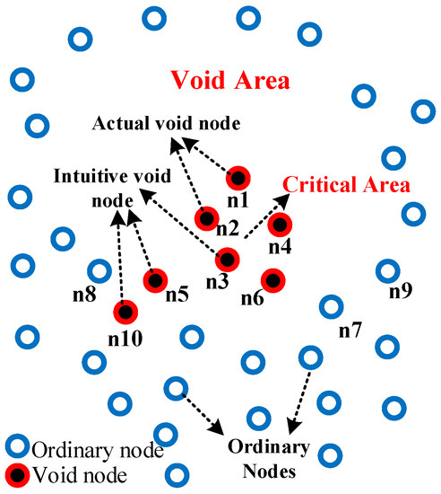
One of the primary challenges in the IoUT environment that has a serious influence on packet delivery ratio and packet drop, especially in sparse networks, is communication void [1,16,17]. Communication void is defined as a problem that occurred if the data packet reaches some areas that did not have any available sensors to forward the data packet. These areas are composed of two types of areas: The void area is the area that did not have any sensors and the critical area is the area that contains the actual void node (i.e., the nodes that did not have any shallower neighbor), intuitive void node (i.e., the nodes that leads the data packet to reach actual void node), or both. Few protocols in UWSN, provide solutions on this topic [17,18,19,20]. To cope with void sensors, current methods employ either geolocation data (location-based) or semi-location information (beacon-based) [13,21]. However, using such methods increase the energy consumption which limits the applicability in the IoUT scenario. Therefore, the void detection technique must be designed to locate void sensors without the use of localization data and to prevent data packets from being sent to the void area during the data forwarding phase to maximize the packet delivery ratio including all network types, especially in wide networks.

In related literature, SPRE-PBR [17] is one of our literature that proposed recently for green computing enabling energy-centric multi-layered concepts. It was recommended by authors to enhance SPRE-PBR to cope with communication void areas. On the other hand, vector-based void avoidance (VBVA) employs the 3D flooding method for identifying the void areas in the network [22]. Moreover, Void-Aware Pressure Routing (VAPR) [23] and the Inherently Void Avoidance Routing (IVAR) [24] uses semi-geo information provided by the sink to identify the void nodes and find the alternate route, which is not practically suitable in most underwater networking applications [7].

In this context, an efficient void aware (EVA) information dissemination routing framework is presented in this paper for enabling IoUT. The framework majorly focuses on identifying a void region in under information dissemination network scenario and subsequently intelligent data forwarding considering the layer-wise classification of the void network region. The major contributions of this paper can be summarized as follows:

• Firstly, underwater network architecture is modeled considering potential void region identification in terms of actual void nodes, intuitive void nodes, and critical network area.
• Secondly, an efficient void aware (EVA) information dissemination framework is presented focusing on void region detection, and intelligent void aware data forwarding technique for the network model.
• Thirdly, the performance of the proposed EVA framework is comparatively evaluated with state-of-the-art techniques considering realistic underwater network scenarios, and related metrics.

The rest of the paper is organized as follows. In Section 2, information dissemination in IoUT is critically reviewed focusing on the strengths and weaknesses of existing protocols for problem identification. The details of the proposed EVA framework are presented in Section 3 consisting of modeling of network architecture, and development of EVA algorithms. The performance evaluation of the proposed EVA framework is discussed in Section 4 considering the comparative analysis of experimental results with the existing techniques.

2. Related Works

In order to have an efficient opportunistic routing protocol, it is paramount to solve many challenges among which is Communication Void (CV) [16,17]. This challenge is faced by the sending nodes when no neighbor node is within its transmission range, which impedes the node from forwarding the packet to the next-hop or destination [25]. Given the dynamic, sparse, and unreliable network topology inherited in Underwater Wireless Sensor Networks (UWSNs), these topologies suffer from high packet loss and low throughput especially if inefficient algorithms are used to handle the void communication problem [25,26]. Needless to say that the adoption of an inefficient void handling algorithm may negatively affect the nodes’ energy consumption and reduce the network lifetime. CV is also a common problem in Territorial Wireless Sensor Networks (TWSNs) [18,27]. However, utilizing the same CV algorithms to UWSNs is not feasible due to the harsh characteristic of these networks. Furthermore, utilizing location-based algorithms for handling CV problems such as Vector-Based Void Avoidance (VBVA) [28], Directional Flooding Routing (DFR) [29], Focused Beam Routing (FBR) [30] are not suitable for UWSNs due to their reliance on acquiring the nodes’ locations utilizing a GPS receiver, which is not feasible in UWSNs [14].

On the other hand, Multi-layer Routing (MRP) [31] protocol proposed a costly architecture that utilizes a super-node to address the CV problem. However, MRP focused on proposing a network architecture but not an efficient routing protocol thus making it not feasible to hand the CV problem [14]. Another algorithm to handle the CV is the Adaptive Power Controlled Routing protocol (APCR) [32]. APCR is an energy-efficient routing protocol that does not mandate any location information of the surrounding nodes. APCR addresses the CV problem by allowing the nodes to adjust their transmission energy in case of not finding a suitable neighbor node thus overcoming the CV problem and achieving a high packets delivery ratio. In contrast, several pressure-based algorithms have been proposed in the literature to handle the CV problem. For example, HydroCast which establishes a detour path between local maximum void nodes with the maximum Expected Packet Advance (EPA) [33]. However, all local maximum neighbor nodes should be aware of each other location information, which is a cost and inefficient process, to forward the packets from each non-neighbor local maximum node.

Void-Aware Pressure Routing (VAPR) protocol proposed in [23] utilizes both the depth and hop-count information to assign UP-DOWN directions to the sink node using the sink node beacon messages. In this protocol, the void node is recognized if the beacon message is received from the deeper node. As such, these nodes are marked as DOWN to prevent them from being part of the packets forwarding process. However, VAPR is not efficient as it relies on the high-cost beacon messages for identifying voice nodes [34]. The Adaptive Mobility of Courier Nodes in Threshold-Optimized DBR Protocol (AMCTD) proposed mobile nodes that can gather packets from void nodes. However, AMCTD neither proposed an algorithm for identifying the void nodes nor demonstrated an efficient algorithm for controlling the movement of the mobile nodes. Finally, the Inherently Void Avoidance Routing (IVAR) [24] tackled the CV problem by allowing all nodes to acquire reachability information throughout the received periodic beacon signals sent by the sink node.

In [35], the authors presented an Opportunistic Void Avoidance Routing (OVAR), a new routing algorithm that addresses the void issue without geo-location information. OVAR can circumvent all types of empty regions at low energy and delay while prioritizing the group of candidate sets. Each forwarding node can conduct a trade-off between energy consumption and packet advancement by altering the number of nodes in its forwarding set, depending on the density of its neighbors. OVAR can also choose any sending nodes from the sender in any direction without containing any hidden information.

In summary, the conducted literature review revealed that most of the proposed UWSNs routing algorithms lack having efficient void handling algorithms to address the CV problem without utilizing the nodes’ location information or the beaconing signal. Therefore, proposing efficient void handling algorithms to solve the CV problem that neither uses the location information nor requires a beacon signal of high importance for developing an energy-efficient pressure-based routing algorithm with low packet loss and high throughput. Therefore, this paper is proposing an efficient void aware routing protocol without relying on the costly nodes’ location information or sink node beacon signal while achieving energy-efficient and reliable forwarding nodes’ selection and suppressing the void nodes from joining the forwarding process.

3. The Proposed Efficient Void Aware Routing Protocol for Enabling Internet of Underwater Things

3.1. Underwater Network Architecture

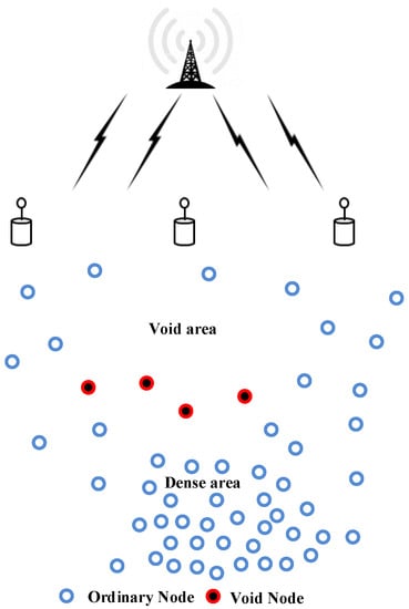
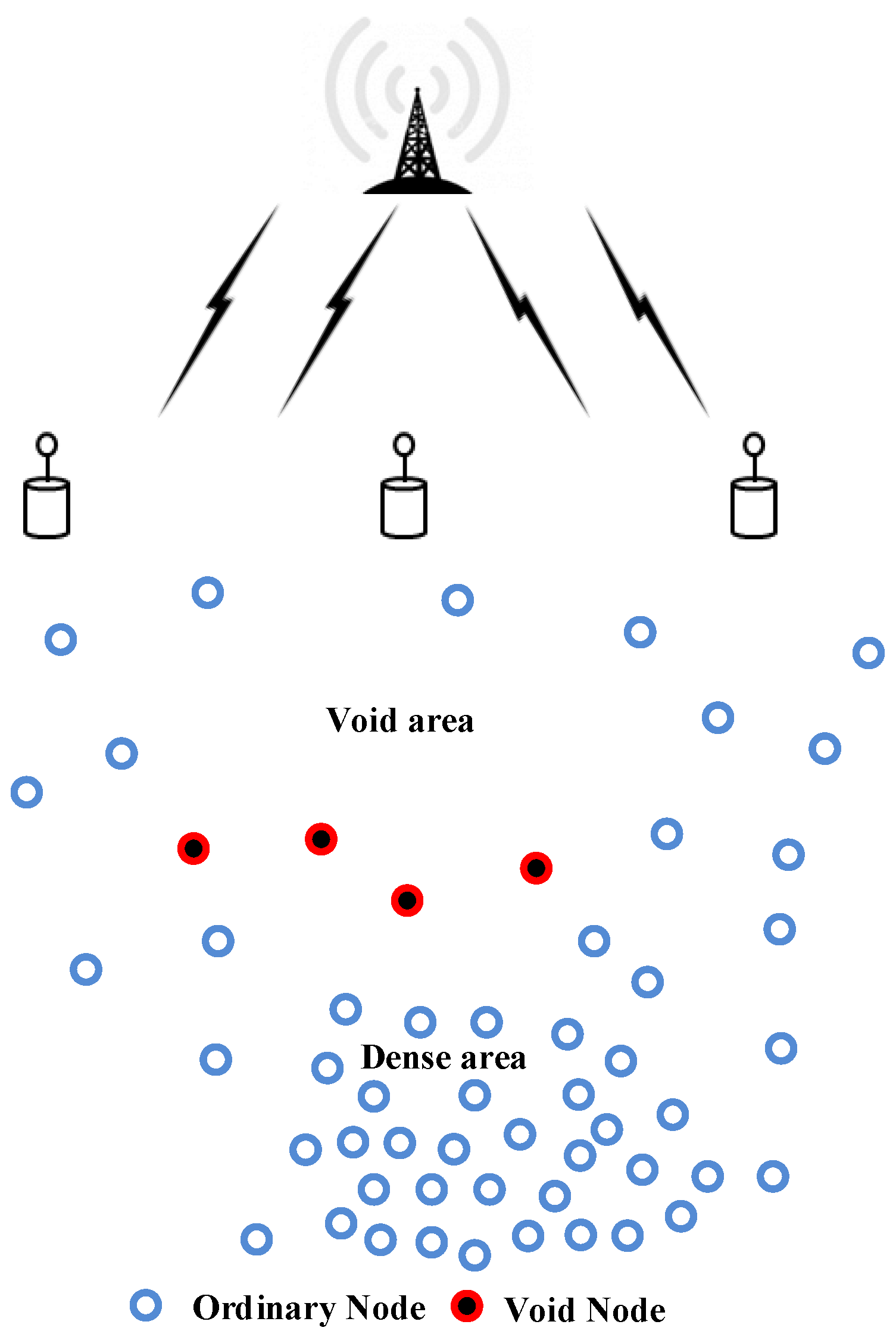
As mentioned in the literature review, the communication void become one of the major issues in opportunistic efficient routing protocols in IoUT, especially in the sparse-based topology network [16,35]. In such topologies, the communication void problem comes during the forwarding process if the forwarder node did not find any shallower next forwarding node. Consequently, it is necessary to design and develop an efficient routing scheme that identifies the void area and avoids forwarding the data packet to the sensors placed in these areas that resulting in minimizing packet loss. Figure 1 illustrates an underwater dynamic network topology that is comprised of dense and void areas and void nodes and ordinary nodes.

Figure 1. Underwater dynamic network topology.

The mechanism of the void detection and handling techniques in WSNs are not efficient to be employed in underwater environments. The void handling techniques in UWSNs are also not efficient in both location-based and beacon-based algorithms. In contrast, existing routing algorithms in the depth-based routing protocols in UWSNs such as DBR [36], EEDBR [37], RE-PBR [11] did not employ void detection algorithms as it taking into account selecting the next forwarding sensor based on either residual energy, depth, or link quality. Moreover, the void handling techniques provided by HydroCast, AMCTD [38], and VAPR have some drawbacks. The utilization of GPS information in HydroCast causes high energy consumption. AMCTD employs courier nodes that move towards the network area to collect the data packet that consumes high energy. The use of beacon messages in the VAPR causes high energy consumption and network overhead. As a result, it is necessary to investigate the void area in depth-based routing protocols without using any external information.

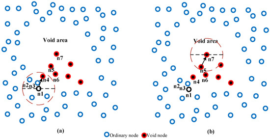
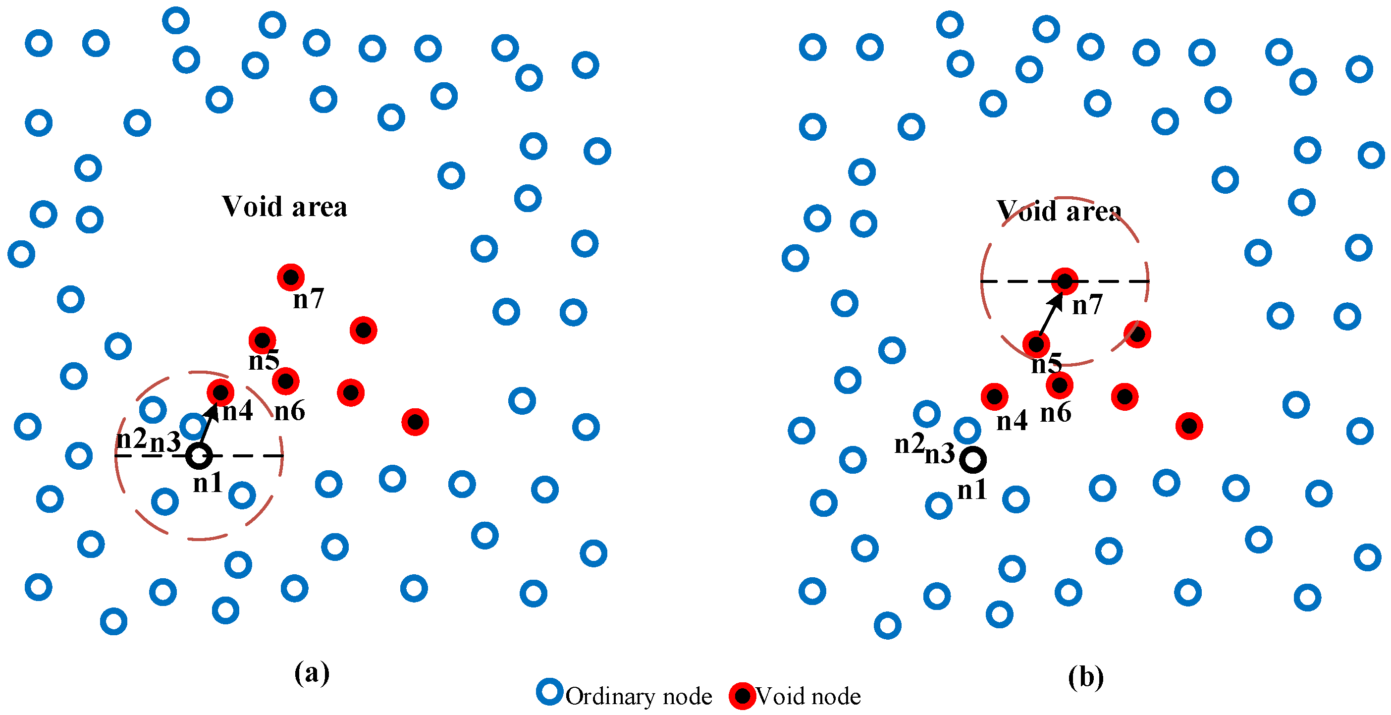
As previously stated in our published algorithms, the RE-PBR and SPRE-PBR algorithms did not deal with void areas. As a result, the chance of packet loss is dramatically increased. Data packet could be lost once it hits the void sensors because the design approach of RE-PBR and SPRE-PBR did not provide any void detection mechanisms. Figure 2 shows an excellent scenario in SPRE-PBR of how the data packet dropped in the sensors in the void area. It is assumed that, as shown in Figure 2a, node $n_1$ shall send a data packet. It thus calls optimal shortest path algorithm to identify the optimal candidate among neighbors $n_2$, $n_3$, and $n_4$. Node $n_1$ then receives the ID of the candidate nodes and picks $n_4$ because it has the best route cost and it adds the ID of the $n_4$ along with the data packet and then broadcasts it to its shallower neighbors. It assumes $n_4$ to have successfully received the data packet and $n_1$ to overhear the received data packet. As $n_5$ and $n_6$ are its candidate set, $n_5$ has the lowest route cost between them and is considered the shortest path in the present hop. The ID of $n_5$ is then embedded with the data packet and forwarded to its shallower neighbors [11,17].

Figure 2. Communication void problem in EVA, (a) optimal route with more neighbour nodes in the range, (b) void problem with limited number of neighbor nodes in the range.

Next, $n_5$ has just one neighbor, as is shown. Thus, $n_6$ as the next transmission node has been picked and the data packet is forwarded to the selected nodes. The following stage is shown in Figure 2b. $n_6$ did not have any candidate set in its routing table. The communication void situation therefore occurs, and in this node, a data packet going to be dropped [11,17].

3.2. Terminology Definition

This section defines terminologies that help in understanding the proposed algorithms and scenarios provided in this paper.

• Void area: the area without any sensors.
• Actual void node: the node $n_i\in U$ that without shallower candidate set in its Routing Table (RT).

  $$(\forall n_i\in U|n_i.RT=\varnothing \Rightarrow n_i\to AcualVoid)$$

  (1)
• Intuitive void node: the node $n_i\in U$ can be considered as an intuitive void node in two scenarios:

If the number of $ActualVoid$ higher than the number of $OrdinaryNode$ in RT and $OrdinaryNode$ does not contain one node at least with “very good” link quality.

$$\begin{array}{c}(\forall n_i\in U\left|n_i.RT\ne \varnothing \&V_{n_i}\ge O_{n_i}\&\&\forall O_{n_i}\in U\right|n_i.RT.distance\ne \\ “VGLink”\Rightarrow n_i\to IntutiveVoid)\end{array}$$

(2)

If the RT is not empty and all candidate sets are $AcualVoid$.

$$(\forall n_i\in U|n_i.RT\ne \varnothing \&S_{n_i}-V_{n_i}=\varnothing \Rightarrow n_i\to IntutiveVoid)$$

(3)

d.

Critical area: the area that contains the actual void node, intuitive void node, or both.

e.

Void node: the node could be identified as a void node if it is an actual or intuitive void node.

$$(\forall n_i\in U|\left(n_i.RT=\varnothing \right)OR(n_i.RT\ne \varnothing \&V_{n_i}\ge O_{n_i}\&\&\forall O_{n_i}\in U|n_i.RT.distance\ne “\mathrm{VGLink}”)OR\left(n_i.RT\ne \varnothing \&S_{n_i}-V_{n_i}=\varnothing \right))$$

(4)

Figure 3 shows the different types of underwater nodes terminology. Node $n_1$ and $n_2$ are an Actual void node because it did not have any shallower neighbors. Node $n_3$, $n_4$, $n_5$, $n_6$, and $n_7$ are Intuitive void node because of two scenarios: (1) node $n_3$, $n_4$, and $n_6$ are Intuitive void nodes because its candidate set is either Actual or Intuitive void node. (2) node $n_5$ and $n_7$ contain void and ordinary nodes as a candidate set in its routing table, but is identified as an Intuitive void node because it assumed that it did not have any ordinary node with “very good link”. As a result, once a data packet reaches one of the mentioned nodes, the data packet could be dropped. The rest of the nodes (i.e., blue nodes) are ordinary and available nodes, meaning that they can forward the data packet with a very high successful delivery ratio.

Figure 3. Different types of nodes in underwater void network scenarios.

3.3. Overview of EVA

In this section, an Efficient Void Aware (EVA) routing protocol is designed and developed to detect the actual and intuitive void nodes and suppress these nodes from the eligibility to forward the data packet. Therefore, SPRE-PBR is enhanced to identify both types of void nodes. Moreover, the data packet forwarding is designed and developed to avoid the void nodes from forwarding the data packets. EVA can professionally deal with selecting the efficient next forwarding nodes with the shortest path and far away from the void or critical areas.

EVA is comprised of three phases, namely data collection, void detection, and data packet forwarding. The data collection in EVA is the same as that proposed in our previous algorithms named RE-PBR and SPRE-PBR that share the main information by broadcasting a hello packet between neighbors within the transmission range. Then, link quality is computed and added to the routing table. In the second phase, the void detection algorithm is designed to identify the actual and intuitive void nodes. The last phase has the responsibility to forward the data packet using the ordinary nodes considering suppressing the void nodes from joining the forwarding process. We want to clarify that the three phases of the execution of the proposed EVA framework are distributed network-wise and sequential in order nodes-wise. It means, the framework is executed in different void network regions in distributed nature. However, at each void node, the three phases including data collection, void node identification, and intelligent data forwarding are executed sequential in order.

3.4. An Efficient Void Aware Routing Protocol: Design Approach

In this section, the EVA routing protocol is described in detail. EVA consists of three phases, namely, data collection, void detection, and data forwarding. This section is structured as follows. First, the routing table and packets used in EVA have been defined. Second, the void detection phase is described in detail. Third, void detection is discussed in detail. Last, the data forwarding phase is explained in detail.

3.4.1. EVA: Tables and Packets Format

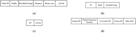
In this section, the Routing Table (RT) and packets have been explained in detail. The RT is the main element of the suggested protocol. Each sensor should gather and store some information for its neighbors within a one-hop range. Each sensor can gather the information through the received hello packet during the data collection phase and void detection phase. As shown in Figure 4a, the RT generally contains six fields including ID, depth value, residual energy, distance (calculated by the triangle metric), route cost (calculated by the triangle metric and residual energy), and Boolean flag (isVoid). The value of this flag has been changed based on the void status of the node (i.e., 0 for void nodes and 1 for ordinary nodes).

Figure 4. Table and packets structure in EVA: (a) routing table, (b) hello packet, (c) probe packet, (d) data packet.

The EVA routing protocol is containing three types of packets: hello, probe and data packets. Hello packets are utilized regularly in the data collection phase to exchange information between neighbors. As demonstrated in Figure 4b, The hello packet is comprised of three fields: ID (for the sender), depth value, and residual energy. ID is employed to verify the sender of the hello packet. Additionally, the depth value is utilized to distinguish the depth level of the sender. The information of the hello packet is extracted in saved in the RT if the sensor received the hello packet from shallower neighbors. Moreover, the residual energy is stored in RT and employed route cost calculation. On the other hand, the void probe packet is presented in the EVA routing protocol to find the void nodes as shown in Figure 4c. This type is containing two fields, namely ID (for the sender) and Boolean isVoid. The first field is the ID of the void node (i.e., actual, and intuitive void node). The probe packet is created by the actual void nodes and transmitted to its one-hop neighbors. If the ID of the receiver node equals the ID of the probe packet in its RT, it changes the isVoid fields in its RT. Then it changes the ID of the probe packet and forwards it if the node discovers itself as an intuitive void node. Otherwise, it discards the probe packet. Figure 4d illustrates the data packet format employed in the suggested protocol. The data packet involves two major elements: packet header and data. The packet header is consisting of four fields, namely Sender ID, packet sequence number, forwarder ID, and source ID. Sender ID is the distinctive ID of the sender node. Packet sequence number the assigned number to the data packets in the source node. Forwarder ID is the ID for the best candidate. Source ID is the ID of the source node that creates the data packets. The last two fields are employed to detect and count the successful data packet dropped or received in the whole network.

3.4.2. Data Collection Phase

Like RE-PBR and SPRE-PBR protocols, each sensor collects the mentioned information from its shallower neighbors by broadcasting a hello packet periodically to its one-hop neighbors including ID, residual energy, and depth. The receiver node stores the information in its RT if the hello packet is received from its shallower level neighbor (defined by depth information). Otherwise, it simply discards the message. Next, each sensor calculates the link quality for all shallower neighbors using the triangle metric algorithm.

3.4.3. Void Detection Phase

This phase is aimed at detecting the actual and initiative void nodes by designing and developing a void detection algorithm. Table 1 shows the notations that used in the void discovery algorithm. In Algorithm 1, each sensor considers itself an actual void node if did not find any sensor in its routing table. The node (i.e.,$n_i$) create a void probe packet containing two fields, called Sender ID and isViod Boolean flag equal to 1 (i.e., True). Then, it inserts its ID and isVoid in the packet and broadcast it to its one-hop neighbor sensors.

Table 1. Notations in the void detection algorithm.

Symbol	Description	Symbol	Description
$n_i$	$i$-th sensor Nodes	$VC$	Void Count Sensors in RT
$id$	Sensor node ID	$OC$	Ordinary count sensors in RT
RT	Routing Table	$dis$	The reliable value in RT
$C$	Candidate set in RT	$RS$	Reliable status = “Very good link”
$vpp$	void probe packet	$RSCount$	The number of “Very good link” in RT
$isVoid$	Boolean Value (True or False)	$senderID$	Sender node ID
loc	The location of the sensor in the RT	$reTime$	Retransmission time
$iv$	Void status in the RT

Secondly, neighbors that receive the probe packet (i.e.,$n_i$) extracts and check the ID and match it with its routing table. If did not find it in the routing table, it drops the packet. Else, it changes the value of isVoid in its routing table to 1. The receiver node then checks whether it is an intuitive void node. It examines two scenarios: first, if all data in the routing table is void nodes, node $n_i$ become an intuitive void. Second, the node (i.e.,$n_i$) check the number of void and ordinary nodes in its routing table. If the void nodes numbers are higher than the ordinary nodes, it checks its routing table if has one ordinary node with a “very good link”. If founds, node $n_i$ become an intuitive void node. It then updates the isVoid value in the packet equal to 1 and updates the ID and rebroadcasts it to its one-hop neighbors. Otherwise, it immediately drops the void probe packet. This method is repeated all sensors updated the isVoid field in the whole network.

The following are the reasons for defining both scenarios as intuitive void nodes. In the first scenario, a node whose neighbors are all void nodes causes the data packet to be dropped since all its neighbors are void nodes, which causes the data packet to be dropped. In the second scenario, a node with a high number of void nodes in its routing table has a higher probability of losing a data packet as most of its neighboring are inside the critical area, causing the data packet to end up at a void node in later hops. As a result, if this node does not have at least one ordinary neighbor with excellent link quality, it is considered unreliable. This causes the data packet to reach the critical area, increasing the chances of losing the data packet, as well as increasing the power consumption of the ordinary neighbors due to the continued employment of these sensors, and causing the ordinary nodes to die early. Furthermore, if this node has at least one ordinary neighbor with very good link quality, it is recognized as an ordinary node since the use of this node could minimize the likelihood of packet loss and causes the data packet to be routed outside from the critical areas’ boundary.

Algorithm 1: EVA: Void Detection Algorithm.
1.	procedure $GenerateVoidProbe$. ($n_i$)
2.	if $Timeout\ge maxTime$ then
3.	if $n_i.RT==\varnothing$ then
4.	Generate $HelloPacket$($vvp$)
5.	$vpp.id\leftarrow n_i.id$
6.	$vpp.isVoid\leftarrow 1$
7.	$\mathrm{Broadcast} vpp$
8.	end if
9.	end if
10.	end procedure
11.	procedure $ReceiveVoidProbe$($n_i , vpp$)
12.	if ($vpp.id\ne$ $n_i.RT$ then
13.	return
14.	else
15.	$loc\leftarrow FindLoc\left(vpp.id , n_i.RT\right)$
16.	$n_i.RT\left[loc\right].iv\leftarrow vpp.isVoid$
17.	end if
18.	$VC\leftarrow 0$
19.	$OC\leftarrow 0$
20.	for $j=1$ to $C$ do
21.	if ($n_i.RT.iv==1$) then
22.	$VC\leftarrow VC+1$
23.	Else
24.	$OC\leftarrow OC+1$
25.	end if
26.	end for
27.	if ($VC==C$) then
28.	$vpp.id\leftarrow n_i.id$
29.	$vpp.isVoid\leftarrow 1$
30.	$\mathrm{Broadcast} vpp$
31.	else if ($VC\ge OC$) then
32.	Let $RS\leftarrow ‘VGLink’$
33.	Let $RSCount\leftarrow 0$
34.	for $j=1$ to $C$ do
35.	if ($n_i.RT\left[j\right].dis==RS$) & ($n_i.RT\left[j\right].iv==0$) then
36.	$RSCount\leftarrow RSCount+1$
37.	end if
38.	end for
39.	if ($RSCount<1$) then
40.	$vpp.id\leftarrow n_i.id$
41.	$vpp.isVoid\leftarrow 1$.
42.	Broadcast $vpp$
43.	end if
44.	else
45.	free ($vpp$)
46.	end if
47.	end procedure

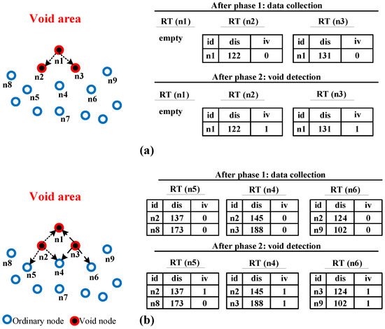
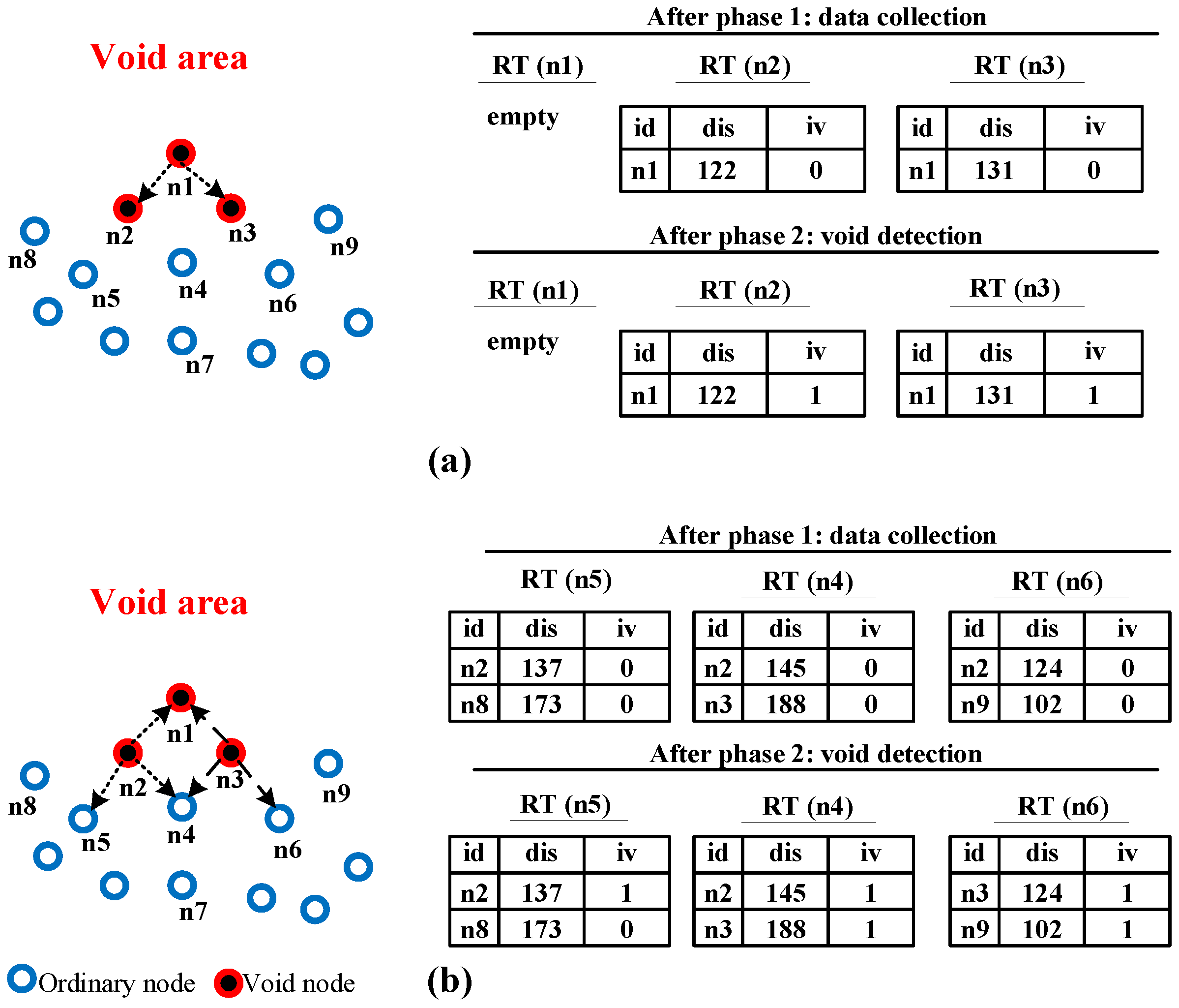
Figure 5 explains the void detection phase of Algorithm 1 in detail. As clearly shown in Figure 5a, node $n_1$ is an actual void node because the RT is empty. Thus, it generates a void probe packet embedded with its ID and isVoid equal to 1 and broadcast it to its one-hop neighbors. Node $n_2$ and $n_3$ obtains this packet because node $n_1$ existed in RT of node $n_2$ and $n_3$. Next, both sensors update its isVoid status in the RT for node $n_1$ equal to 1. Consequently, node $n_2$ and $n_3$. become an intuitive void node as all its neighbors in RT are void nodes. Therefore, these nodes embedded their ID and update the isVoid field in the probe packet and rebroadcast it to its one-hop neighbors.

Figure 5. Underwater void node detection execution, (a) Empty RT, and (b) Full RT scenario.

In Figure 5b, node $n_1$, $n_4$, and $n_5$ collects the packet from node $n_2$. Node $n_1$ simply drops the packet because it is not available in its RT. Node $n_4$ and $n_5$ accept the packet as a node $n_2$ are clearly inside the RT of the node $n_4$ and $n_5$. Therefore, it changes the value of isVoid in the RT of node $n_2$ equal to 1. Here, the number of void nodes is equal to the number of the ordinary nodes and there is at least one node with high link quality (i.e., node $n_8$ in the RT of node $n_5$ and node $n_3$ in the RT of node $n_4$), node $n_5$ and $n_4$ become an ordinary node. Therefore, they simply discard the packet. On the other hand, node $n_1$, $n_4$, and $n_6$ gets the packet from node $n_3$. Node $n_1$ simply drop the packet because node $n_3$ is not in the RT of $n_1$. Additionally, node $n_4$ and $n_6$ extract the packet because node $n_3$ is inside the RT of node $n_4$ and $n_6$. Thus, node $n_4$ and $n_6$ change the status of isVoid equal to 1 for node $n_3$ in their RT. Here, all neighbors in the RT of the node $n_4$ are void nodes, node $n_4$ become an intuitive void node. Node $n_4$ then change the ID of the void probe packet and the status of is isVoid equal to 1 and rebroadcast it to its one-hop neighbors. Moreover, node $n_6$ is an intuitive void node because it does not have an ordinary node with high link quality. Therefore, node $n_6$ change the ID and the isVoid in the probe packet and rebroadcast it. This method is repeated continuously until all sensors become aware of its void status whether void or ordinary nodes.

3.4.4. Data Forwarding Phase

In this phase, the data forwarding algorithm is designed to select the non-void nodes in the process of forwarding the data packet. Here, the data forwarding method in SPRE-PBR is modified to suppress the void nodes in joining the forwarding process. The OSPA algorithm proposed in SPRE-PBR is enhanced to select the best candidate from the ordinary nodes with ignoring both cases of void nodes mentioned previously. All sensors have enough information collected from both phases one and two. This information has been utilized to select the efficient void aware candidate sensor among neighbors. In this phase, once a sensor has data to send it to calculate the route cost based on the triangle metric for all neighbors and store it in the routing table. Then, the best candidate has been selected based on the non-void sensors with high link quality. Table 2 shows the notations that are used in the efficient void aware data forwarding algorithms.

Table 2. Notations in void aware data forwarding.

Symbol	Description	Symbol	Description
$R$	Transmission Range	$VC$	Void count sensors in RT
$C$	Candidate set in NIT	$n_i$	$i$-th sensor nodes, $1\le i\le N$
$BestN$	Best neighbors	$RT$	Routing Table
EN	The number of eligible sensors in EVA-DF	$id$	Sensor node ID
$DepthDiff$	Depth differences between sender and receiver	$OCSet$	Set of ordinary neighbors in EVA-DF
$depth$	Depth value	$RCost$	The route cost field in the data packet
$iv$	Void status in the RT	$Threshold$	The highest number of the best candidate set

Algorithm 2 illustrates how the modified algorithm named Efficient Void Aware Data Forwarding (EVA-DF) algorithm chooses the best efficient candidate among neighbors. This algorithm consists of one procedure and one method. Firstly, line 13–41 (EVA-DF) is designed to select the set of candidate neighbors from the ordinary nodes in the highest layer. Secondly, line 1–12 Procedure $LayerClassification$ is designed to distinguish the number of best candidates set among neighbors in the RT based on the efficient non-void sensors. The rest of the methods have been briefly described in SPRE-PBR. As a result, the EVA-DF is normally called by the data forwarding algorithm to select the efficient void aware sensor nodes that have a direct impact on increasing the packet delivery ratio.

Algorithm 2: EVA: Efficient Void Aware Data Forwarding.
1:	procedure $LayerClassification$($n_i, R1, R2, BestN, EN, OCSet$)
2:		$j\leftarrow 1$
3:		while $\mathrm{EN}<BestN and j\le C$
4:			$depthDiff\leftarrow \left|n_i.depth|-|n_i.RT\left[j\right].depth\right|$
5:			if ($n_i.RT\left[j\right].iv==0$) and ($R1<depthDiff\le R2$) then
6:				$EN\leftarrow \mathrm{EN}+1$
7:				$OCSet\left[EN\right]\leftarrow n_i.RT\left[j\right].id$
8:			end if
9:			$j\leftarrow j+1$
10:		end while
11:	end procedure
12:
13:	methodEVA-DF ($n_i$)
14:		Sort $n_i.RT$ based on $n_i.RT.RCost$ in ascending order
15:		Let $BestN\leftarrow 0$
16:		Let $VC\leftarrow 0$
17:		for $j=1$ to $C$ do
18:			if ($n_i.RT\left[j\right].iv==1$) then
19:				$VC\leftarrow VC+1$
20:			end if
21:		end for
22:		if ($C-VC>Threshold$) then
23:			$BestN\leftarrow Threshold$
24:		else
25:			if $C-VC\le Threshold$then
26:				$BestN\leftarrow C-VC$
27:			end if
28:		end if
29:		Clear ($OCSet$)
30:		Let $EN\leftarrow 0$
31:		if $EN<BestN$then
32:			$LayerClassification$ ($n_i,\frac{2R}{3},R,BestN, EN,OCSet$)
33:		end if
34:		if $EN<BestN$then
35:			$LayerClassification$ ($n_i,\frac{R}{3},\frac{2R}{3},BestN, EN,OCSet$)
36:		end if
37:		if $EN<BestN$then
38:			$LayerClassification$ ($n_i,0,\frac{R}{3},BestN, EN,OCSet$)
39:		end if
40:		return$OCSet$
41:	end method

4. Results and Discussion

In this section, we examine the results of the EVA routing protocol. Then we compare the proposed EVA with well-known related routing schemes named VAPR and SPRE-PBR.

4.1. Simulation Setting

In this section, the performance of EVA has been calculated using Network Simulator 2 (NS2) with the AquaSim package for underwater [39]. The random topology with various number of sensors have been employed (i.e., $25-400$) with a high level are of $1250 {\mathrm{m}}^3$. The transmission range has been set equal to $250 \mathrm{m}$ as it basically appropriates for such underwater networking applications and the initial energy is assigned to $100 \mathrm{J}$ with $15 \mathrm{s}$ packet generation time and size is 64 bytes. On the other hand, the hello packet interval is equal to $100\mathrm{s}$ the energy model has been employed using the same that employed in our published protocols. The energy consumption in terms of transmitting, receiving, and idle listening is set to ($2\mathrm{w},0.75\mathrm{w},\mathrm{and}8\mathrm{mw}$) [11,14,17]. A Broadcast MAC has been employed as a Media Access Control (MAC) [40]. We want to highlight that the result has been averaged from 50 runs for the whole performance evaluation at the same time. This could help in extracting the results for all performance evaluations in the same situation and highlighting them as error bars in the result figures. Table 3 below shows the mentioned setting clearly.

Table 3. Simulation sitting.

Simulation Parameter	Values
Number of sensor nodes	50–400
Network topology	Random topology
Deployment area	$1250{\mathrm{m}}^3$
Bandwidth	$10\mathrm{Kbps}$
Communication medium	Acoustic Waves
Area of transmission range	$250$ m
MAC protocol	$BrodcastMAC$
Node movement	0–3$\mathrm{m}/\mathrm{s}$
Hello packet interval	$100\mathrm{s}$
Data packet size	$64$ bytes
Initial energy	$100\mathrm{J}$
Power consumption	$2\mathrm{w},0.75\mathrm{w},\mathrm{and}8\mathrm{mw}$
Packet generation time	$15\mathrm{s}$
Number of Runs	50

4.2. Performance Metrics

In UWSNs, the four main performance metrics that are usually used in evaluating the performance of the well-known algorithms have been utilized in our algorithms examined below:

• Energy Consumption: the amount of energy consumed for each sensor.
• Packet Delivery Ratio: the ratio of the successfully delivered packets to the sink divided by the number of total transmitted packets by each sensor.
• Network Lifetime: the major lifetime that has been measured based on the first die sensor in the network.
• End-to-End Delay: the average delay caused by each sensor during the forwarding process.

4.3. Analysis of Results

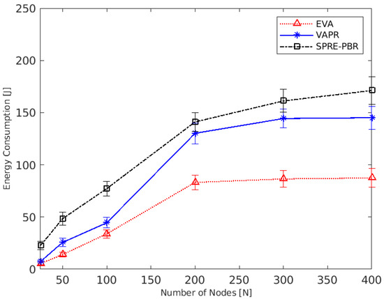
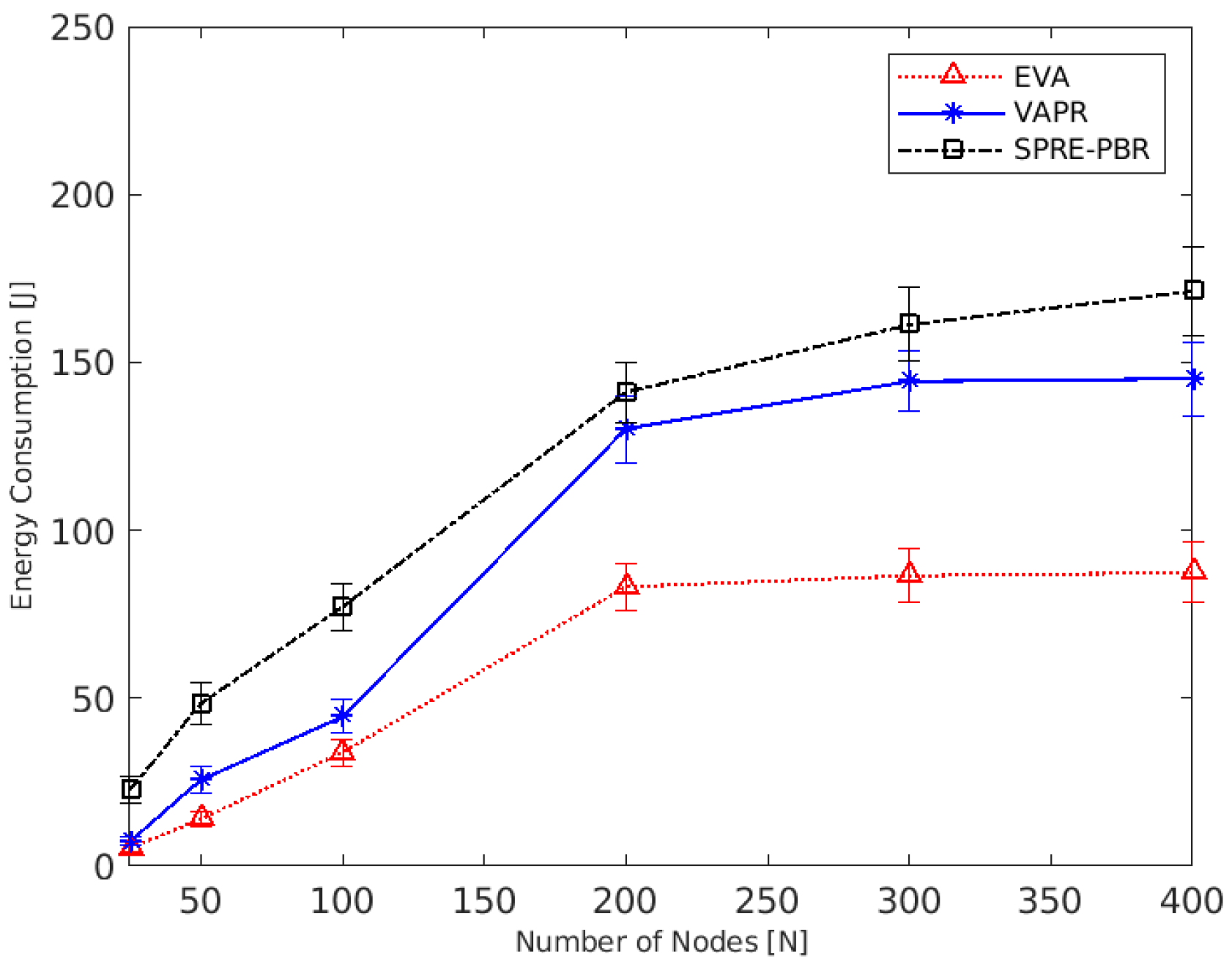
This section discusses the result of the proposed algorithm comparatively with well-known algorithms called VAPR [23] and SPRE-PBR [17]. Figure 6 below shows the impact of increasing the number of sensors in terms of energy consumption. As illustrated in the figure below, the energy consumption is increased with increasing the number of sensors. The energy consumption of EVA is lower than VAPR and SPRE-PBR for some reasons: the employment of route cost during the forwarding phase helps in selecting the next forwarding nodes with lower energy and link quality among neighbors. Moreover, the use of the introduced void detection algorithm can efficiently suppress the void nodes from forwarding the data packets. In comparison with VAPR, the void aware method consumes high energy as the assignment of the directions in VAPR consumes more energy for beaconing messages that supplied by the sink. Furthermore, SPRE-PBR consumes high energy as it did not provide a solution to avoid the void nodes that could be selected many times, and data could reach the trap area. Furthermore, the employment of the introduced EVA-DF has a direct impact on reducing the energy consumption because the number of the candidate set is dynamically reduced, leading to avoiding the unreliable and void sensors joining the forwarding process. With increasing the number of nodes equal to 200, the energy consumption of EVA is reduced by about 14% and 42% compared to SPRE-PBR and VAPR.

Figure 6. Comparison of EVA with existing algorithms in terms of energy consumption.

On the other hand, the energy consumption with a different number of sensors in VAPR and SPRE-PBR is dramatically increased with increasing the number of nodes. The reason for that is the VAPR void detection algorithm uses direction up/down technique, leading to select the sensors without considering the shortest path as some data packet needs to be forwarded to deeper sensors, and SPRE-PBR did not provide any solution for the communication void problem. These reasons cause high energy consumption.

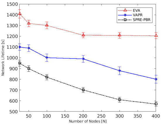
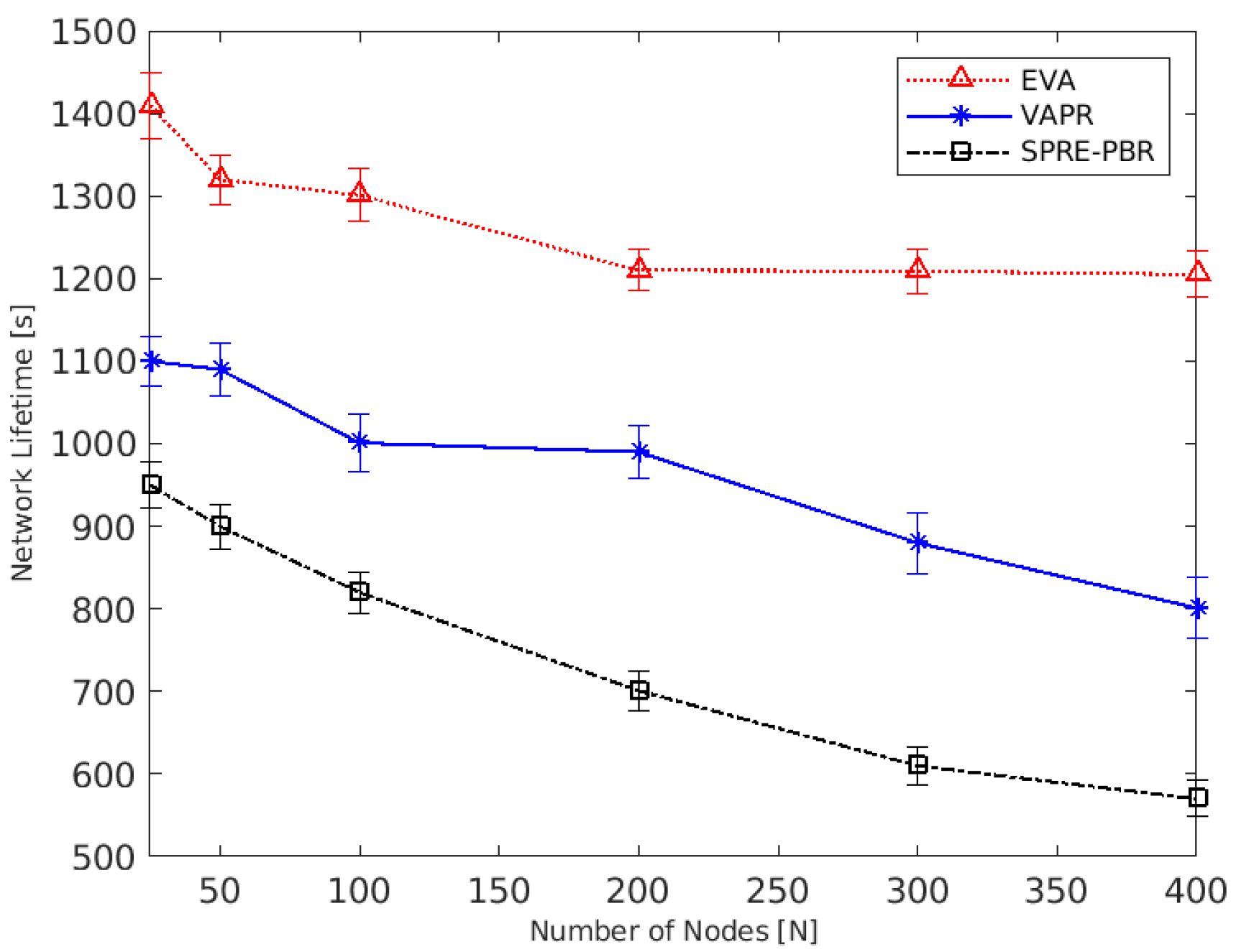
Figure 7 shows the effect of increasing the number of nodes on network lifetime in VAPR, SPRE-PBR, and EVA. When compared with other methods, the displayed results demonstrate that EVA has the best network lifetime. This is since route cost calculation uses minimum energy to optimize energy consumption and link quality, allowing the network lifetime to be maximized. Furthermore, the use of layering technique in the EVA-DF algorithm aids in the selection of the fastest distance while considering the route cost for each ordinary node, resulting in lower energy consumption and increased network lifetime. As a result, the data packets take the shortest path to the sink while balancing power usage. Consequently, the network lifetime has increased dramatically.

Figure 7. Comparison of EVA with existing algorithms in terms of network lifetime.

The network lifetime is decreasing with increasing numbers of sensors of VAPR and SPRE-PBR, as illustrated in Figure 7. In most cases, VAPR has high network life than SPRE-PBR and less than EVA. The reason is that VAPR uses 2-hop knowledge to pick the fastest route. However, the performance of finding the shortest route based on 2-hop knowledge is influenced by high-density networks, which reduces the lifetime of the network. In turn, EVA achieves stabilized network lifetime compared with other methods, with an expanding number of sensors. This is since the EVA-DF method may effectively work with any number of sensors by finding the shortest route while discarding node energy. Therefore, the energy is controlled by employing residual energy, and the hop count is minimized by stacking the forwarding region and improving link quality. As a result, the network lifetime is extended.

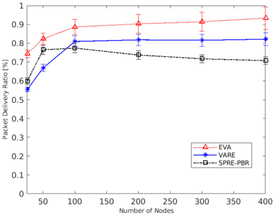
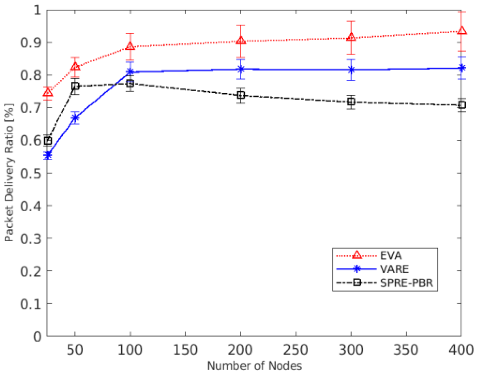
Figure 8 depicts the effect of increasing the number of nodes in EVA on the packet delivery ratio, as well as a comparison to SPRE-PBR and VAPR. The results show that the packet delivery ratio in SPRE-PBR, VAPR, and EVA is increased with the growing number of sensors. In comparison to other techniques, EVA had the highest packet delivery ratio. The reason is that EVA works with successful packet delivery efficiently by using link quality to calculate route costs, reliable efficient shortest route mechanism, and void avoidance method. For example, the route cost computation chooses the sensor of high residual energy and good link quality, balancing energy consumption, establishing stable links, and guaranteeing the delivery ratio. The EVA-DF method will choose the fastest paths and prevent redundant forwarding, reducing the total amount of data packets transmitted while maintaining a suitable packet delivery ratio. Finally, void detection and avoidance routing algorithms are used to prevent void sensors, while selecting the best nodes improves the packet delivery ratio, which is especially important in sparse networks.

Figure 8. Comparison of EVA with existing algorithms in terms of packet delivery ratio.

As shown in Figure 8, increasing the number of sensors to 50 increases the packet delivery ratio in EVA by around 8% and 5%, accordingly, when compared to VAPR and SPRE-PBR. Furthermore, increasing the number of sensors to 400 increases the packet delivery ratio for EVA to around 96%, implying that EVA achieves a better packet delivery ratio than SPRE-PBR and VAPR, which have packet delivery ratios of 4% and 2%, accordingly. Furthermore, the findings demonstrate that VAPR achieves a good packet delivery ratio comparable to EVA, although it consumes roughly 34% less energy than VAPR in the same situation.

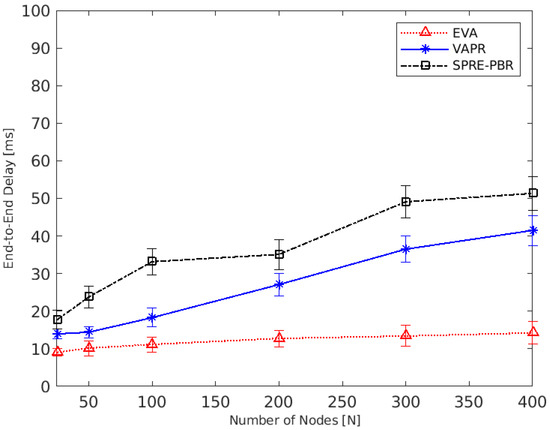
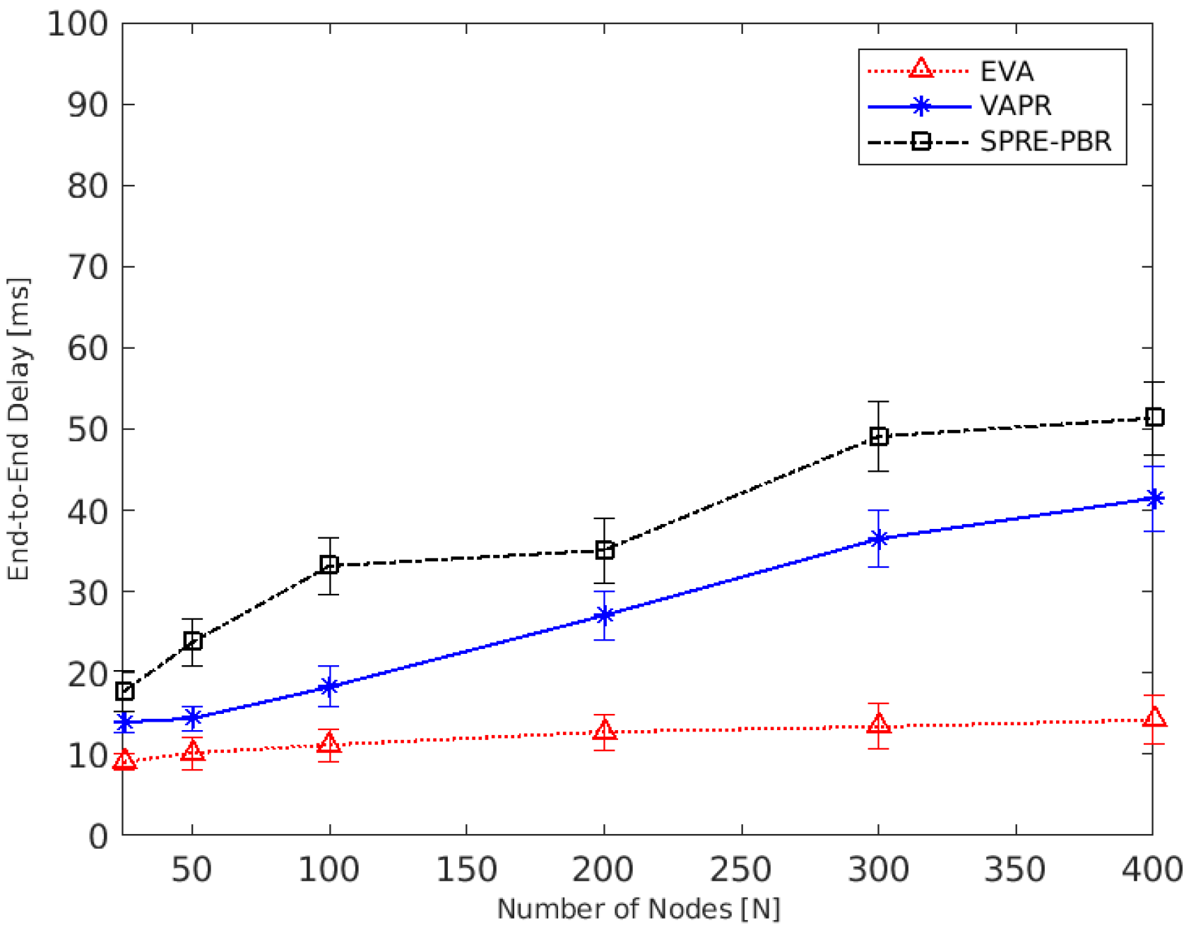
Figure 9 shows the efficiency of the proposed algorithms compared to VAPR and SPRE-PBR in terms of end-to-end delay. The use of the EVA-DF algorithm has a direct impact on reducing the delay. This is because it avoids the void nodes (i.e., once the data reach the void node, it causes some delay because of the use of the retransmission mechanism). Moreover, the use of sender-based techniques reduces the delay since the data forwarding phase did not employ a holding technique, meaning that the data packet will be broadcast directly to its one-hop neighbors. With increasing the number of sensors, the delay is increased as with increasing the number of nodes, the chance of retransmission techniques may be increased. For instance, with increasing the number of nodes to 300, the delay of EVA is decreased compared to VAPR and SPRE-PBR about 41% and 63%, respectively.

Figure 9. Comparison of EVA with existing algorithms in End-to-End Delay.

It is remarkable as shown in Table 4 that the EVA framework outperforms SPRE-PBR 56.6% less in terms of energy consumption, 21.4% increase in packet delivery ratio, 72.7% increase in network lifetime, and 63.5% decrease in delay in the presence of a different number of nodes. On the other hand, the EVA outperforms VAPR in terms of Packet delivery ratio is 17.2% increase, 47.4% decrease in terms of delay and 36% decrease in energy consumption, and a 31.5% increase in terms of network lifetime as shown in Table 2. We do agree that the performance of the proposed EVA is very close to the VAPR in terms of network lifetime. However, it is noted that the suggested framework’s total performance gains are considerable and obvious for wide area networks or with increasing the number of sensors in the network. As a result, we believe that in a realistic traffic environment, performance gains will be significant. We do realize that with 200 nodes, the end-to-end delay performance of SPRE-PBR did increase in a similar ratio as it was the case for 150 nodes and 250 nodes. However, we want to clarify that this is due to the average case scenario for drawing the results where we took 50 simulation runs for the similar network setting for each result data in our drawing.

Table 4. Performance Analysis of EVA against competitive protocols with increase ↑ or decrease ↓ trend.

					% Improvements of EVA as Compared with Existing Techniques
	Nodes	VAPR	SPRE-PBR	EVA	% Improvement of EVA as Compared with SPRE-PBR	% Improvement of EVA as Compared with VAPR
Node vs. Energy Consumption (J)	25	7.2987	22.5984	5.3852	76.1699943	26.2169975
	50	25.6574	48.3955	13.9745	71.1243814	45.5342318
	100	44.4363	77.1954	33.8731	56.1203129	23.7715561
	200	140.2047	141.1042	83.1745	41.054554	40.6763825
	300	144.3546	161.2050	86.4730	46.3583636	40.0968171
	400	145.1486	171.1740	87.4040	48.938507	39.7830913
	Average % Improvements				56.6276855 ↓	36.0131794 ↓
Node vs. Packet Delivery Ratio (%)	25	0.5531	0.5981	0.7429	24.21	34.3156753
	50	0.6684	0.7647	0.8233	7.663136	23.1747457
	100	0.8088	0.7739	0.8862	14.51092	9.56973294
	200	0.8177	0.7371	0.9027	22.46642	10.3950104
	300	0.8155	0.7171	0.9135	27.38809	12.0171674
	400	0.8211	0.7072	0.9333	31.97115	13.6645963
	Average % Improvements				21.36829 ↑	17.189488 ↑
Node vs. Network Lifetime (Sec)	25	1100	950	1410	48.42105	28.1818182
	50	1090	900	1320	46.66667	21.1009174
	100	1001	820	1301	58.65854	29.97003
	200	990	701	1210	72.61056	22.2222222
	300	880	610	1209	98.19672	37.3863636
	400	801	570	1205	111.4035	50.4369538
	Average % Improvements				72.65951 ↑	31.5497175 ↑
Node vs. End-to-End Delay (ms)	25	13.9620	17.6721	9.0468	48.80744	35.2041255
	50	14.3984	23.7532	10.1746	57.16535	29.3352039
	100	18.2798	33.1678	11.1706	66.32095	38.8910163
	200	27.0748	35.1045	12.7658	63.63486	52.8498825
	300	36.5000	49.1000	13.4010	72.70672	63.2849315
	400	41.4862	51.3475	14.2354	72.27635	65.686421
	Average % Improvements				63.48528 ↓	47.5419301 ↓

5. Conclusions and Future Work

In this paper, an efficient void aware framework for information dissemination in the underwater network is presented. The framework development started with underwater network architecture modeling considering the existence of a void network region during continuous operation or monitoring in the IoUT environment. Subsequently, a stepwise strategy has been developed for precisely identifying void network regions in the underwater scenario. To avoid the void region during information dissemination, an intelligent data forwarding algorithm has been developed utilizing the knowledge void region. A comparative performance evaluation of the proposed framework has confirmed the underwater network metrics-centric benefits of the proposed EVA framework in comparison with the recent state-of-the-art techniques. Summary of benefits has been presented in Table 2. The team of authors in this paper are well engaged in the IoUT research and developments in the last five years. Towards extending this research in the future, authors will explore the development of an edge computing-based framework for intelligent void region identification and handling. How solar-powered tiny drones can improve the performance of the IoUT environment will also be the quest of our future research.

References

- Ayaz, M.; Baig, I.; Abdullah, A.; Faye, I. A survey on routing techniques in underwater wireless sensor networks. J. Netw. Comput. Appl. 2011, 34, 1908–1927. [Google Scholar] [CrossRef] [Scilit]
- Domingo, M.C. An overview of the internet of underwater things. J. Netw. Comput. Appl. 2012, 35, 1879–1890. [Google Scholar] [CrossRef] [Scilit]
- Kao, C.-C.; Lin, Y.-S.; Wu, G.-D.; Huang, C.-J. A Comprehensive Study on the Internet of Underwater Things: Applications, Challenges, and Channel Models. Sensors 2017, 17, 1477. [Google Scholar] [CrossRef] [Scilit]
- Kumar, V.; Kumar, S.; AlShboul, R.; Aggarwal, G.; Kaiwartya, O.; Khasawneh, A.; Lloret, J.; Al-Khasawneh, M. Grouping and Sponsoring Centric Green Coverage Model for Internet of Things. Sensors 2021, 21, 3948. [Google Scholar] [CrossRef] [Scilit]
- Liou, E.-C.; Kao, C.-C.; Chang, C.-H.; Lin, Y.-S.; Huang, C.-J. Internet of underwater things: Challenges and routing protocols. In Proceedings of the 2018 IEEE International Conference on Applied System Invention (ICASI), Chiba, Japan, 13–17 April 2018; pp. 1171–1174. [Google Scholar]
- Jouhari, M.; Ibrahimi, K.; Tembine, H.; Ben-Othman, J. Underwater Wireless Sensor Networks: A Survey on Enabling Technologies, Localization Protocols, and Internet of Underwater Things. IEEE Access 2019, 7, 96879–96899. [Google Scholar] [CrossRef] [Scilit]
- Song, Y. Underwater Acoustic Sensor Networks with Cost Efficiency for Internet of Underwater Things. IEEE Trans. Ind. Electron. 2020, 68, 1707–1716. [Google Scholar] [CrossRef] [Scilit]
- Khalifeh, A.; Darabkh, K.A.; Khasawneh, A.M.; Alqaisieh, I.; Salameh, M.; Alabdala, A.; Alrubaye, S.; Alassaf, A.; Al-Hajali, S.; Al-Wardat, R.; et al. Wireless Sensor Networks for Smart Cities: Network Design, Implementation and Performance Evaluation. Electronics 2021, 10, 218. [Google Scholar] [CrossRef] [Scilit]
- Zhou, Z.; Yao, B.; Xing, R.; Shu, L.; Bu, S. E-CARP: An Energy Efficient Routing Protocol for UWSNs in the Internet of Underwater Things. IEEE Sens. J. 2015, 16, 4072–4082. [Google Scholar] [CrossRef] [Scilit]
- Coutinho, R.W.L.; Boukerche, A.; Loureiro, A.A. A novel opportunistic power controlled routing protocol for internet of underwater things. Comput. Commun. 2019, 150, 72–82. [Google Scholar] [CrossRef] [Scilit]
- Khasawneh, A.; Latiff, M.S.B.A.; Kaiwartya, O.; Chizari, H. A reliable energy-efficient pressure-based routing protocol for underwater wireless sensor network. Wirel. Netw. 2018, 24, 2061–2075. [Google Scholar] [CrossRef] [Scilit]
- Mhemed, R.; Comeau, F.; Phillips, W.; Aslam, N. Void Avoidance Opportunistic Routing Protocol for Underwater Wireless Sensor Networks. Sensors 2021, 21, 1942. [Google Scholar] [CrossRef] [Scilit]
- Khasawneh, A.; Latiff, M.S.B.A.; Kaiwartya, O.; Chizari, H. Next Forwarding Node Selection in Underwater Wireless Sensor Networks (UWSNs): Techniques and Challenges. Information 2017, 8, 3. [Google Scholar] [CrossRef] [Scilit]
- Khasawneh, A.M.; Kaiwartya, O.; Lloret, J.; Abuaddous, H.Y.; Abualigah, L.; Al Shinwan, M.; Al-Khasawneh, M.A.; Mahmoud, M.; Kharel, R. Green Communication for Underwater Wireless Sensor Networks: Triangle Metric Based Multi-Layered Routing Protocol. Sensors 2020, 20, 7278. [Google Scholar] [CrossRef] [Scilit]
- Alfouzan, F.; Shahrabi, A.; Ghoreyshi, S.M.; Boutaleb, T. A Comparative Performance Evaluation of Distributed Collision-free MAC Protocols for Underwater Sensor Networks. In Proceedings of the 8th International Conference on Sensor Networks, Prague, Czech Republic, 26–27 February 2019; pp. 85–93. [Google Scholar] [CrossRef] [Scilit]
- Khasawneh, A.M.; Abualigah, L.; Al Shinwan, M. Void Aware Routing Protocols in Underwater Wireless Sensor Networks: Variants and challenges. J. Phys. Conf. Ser. 2020, 1550, 032145. [Google Scholar] [CrossRef] [Scilit]
- Khasawneh, A.M.; Kaiwartya, O.; Khalifeh, A.; Abualigah, L.M.; Lloret, J. Green Computing in Underwater Wireless Sensor Networks Pressure Centric Energy Modeling. IEEE Syst. J. 2020, 14, 4735–4745. [Google Scholar] [CrossRef] [Scilit]
- Khasawneh, A.; Bin Abd Latiff, M.S.; Chizari, H.; Tariq, M.; Bamatraf, A. Pressure based routing protocol for underwater wireless sensor networks: A survey. KSII Trans. Internet Inf. Syst. (TIIS) 2015, 9, 504–527. [Google Scholar] [CrossRef]
- Rehman, Z.U.; Iqbal, A.; Yang, B.; Hussain, T. Void Hole Avoidance Based on Sink Mobility and Adaptive Two Hop Vector-Based Forwarding in Underwater Wireless Sensor Networks. Wirel. Pers. Commun. 2021, 120, 1417–1447. [Google Scholar] [CrossRef] [Scilit]
- Alfouzan, F.A.; Shahrabi, A.; Ghoreyshi, S.M.; Boutaleb, T. A Collision-Free Graph Coloring MAC Protocol for Underwater Sensor Networks. IEEE Access 2019, 7, 39862–39878. [Google Scholar] [CrossRef] [Scilit]
- Kanthimathi, N. Void handling using Geo-Opportunistic Routing in underwater wireless sensor networks. Comput. Electr. Eng. 2017, 64, 365–379. [Google Scholar] [CrossRef] [Scilit]
- Xie, P.; Zhou, Z.; Peng, Z.; Cui, J.-H.; Shi, Z. Void Avoidance in Three-Dimensional Mobile Underwater Sensor Networks. In Proceedings of the International Conference on Wireless Algorithms, Honolulu, HI, USA, 24–26 June 2009; pp. 305–314. [Google Scholar] [CrossRef] [Scilit]
- Noh, Y.; Lee, U.; Wang, P.; Choi, B.S.C.; Gerla, M. VAPR: Void-Aware Pressure Routing for Underwater Sensor Networks. IEEE Trans. Mob. Comput. 2012, 12, 895–908. [Google Scholar] [CrossRef] [Scilit]
- Ghoreyshi, S.M.; Shahrabi, A.; Boutaleb, T. An inherently void avoidance routing protocol for underwater sensor networks. In Proceedings of the 2015 International Symposium on wireless communication systems (ISWCS), Brussels, Belgium, 25–28 August 2015; pp. 361–365. [Google Scholar]
- Sher, A.; Khan, A.; Javaid, N.; Ahmed, S.H.; Aalsalem, M.Y.; Khan, W.Z. Void Hole Avoidance for Reliable Data Delivery in IoT Enabled Underwater Wireless Sensor Networks. Sensors 2018, 18, 3271. [Google Scholar] [CrossRef] [Scilit]
- Alfouzan, F. Energy-Efficient Collision Avoidance MAC Protocols for Underwater Sensor Networks: Survey and Challenges. J. Mar. Sci. Eng. 2021, 9, 741. [Google Scholar] [CrossRef] [Scilit]
- Al-Shalabi, M.; Anbar, M.; Wan, T.-C.; Khasawneh, A. Variants of the Low-Energy Adaptive Clustering Hierarchy Protocol: Survey, Issues and Challenges. Electronics 2018, 7, 136. [Google Scholar] [CrossRef] [Scilit]
- Ibrahim, D.M.; Eltobely, T.E.; Fahmy, M.M.; Sallam, E.A. Enhancing the vector-based forwarding routing protocol for underwater wireless sensor networks: A clustering approach. In Proceedings of the International Conference on Wireless and Mobile Communications, Seville, Spain, 22–26 June 2014; pp. 98–104. [Google Scholar]
- Hwang, D.; Kim, D. DFR: Directional flooding-based routing protocol for underwater sensor networks. In Proceedings of the OCEANS 2008, Quebec City, QC, Canada, 15–18 September 2008; pp. 1–7. [Google Scholar] [CrossRef] [Scilit]
- Jornet, J.M.; Stojanovic, M.; Zorzi, M. Focused beam routing protocol for underwater acoustic networks. In Proceedings of the Third ACM International Workshop on Underwater Networks, San Francisco, CA, USA, 15 September 2008; pp. 75–82. [Google Scholar]
- Wahid, A.; Lee, S.; Kim, D.; Lim, K.-S. MRP: A Localization-Free Multi-Layered Routing Protocol for Underwater Wireless Sensor Networks. Wirel. Pers. Commun. 2014, 77, 2997–3012. [Google Scholar] [CrossRef] [Scilit]
- Al Bzoor, M.; Zhu, Y.; Liu, J.; Ammar, R.; Cui, J.H.; Rajasekaran, S. An adaptive power controlled routing protocol for underwater sensor network. Int. J. Sens. Netw. 2015, 18, 238. [Google Scholar] [CrossRef] [Scilit]
- Noh, Y.; Lee, U.; Lee, S.; Wang, P.; Vieira, L.F.M.; Cui, J.-H.; Gerla, M.; Kim, K. HydroCast: Pressure Routing for Underwater Sensor Networks. IEEE Trans. Veh. Technol. 2015, 65, 333–347. [Google Scholar] [CrossRef] [Scilit]
- Ganesh, N. Performance Evaluation of Depth Adjustment and Void Aware Pressure Routing (DA-VAPR) Protocol for Underwater Wireless Sensor Networks. Comput. J. 2019, 63, 193–202. [Google Scholar] [CrossRef] [Scilit]
- Ghoreyshi, S.M.; Shahrabi, A.; Boutaleb, T. An opportunistic void avoidance routing protocol for underwater sensor networks. In Proceedings of the 2016 IEEE 30th International Conference on Advanced Information Networking and Applications (AINA), Crans-Montana, Switzerland, 23–25 March 2016; pp. 316–323. [Google Scholar]
- Yan, H.; Shi, Z.J.; Cui, J.-H. DBR: Depth-based routing for underwater sensor networks. In Proceedings of the International Conference on Research in Networking, Singapore, 5–9 May 2008; pp. 72–86. [Google Scholar]
- Wahid, A.; Kim, D. An Energy Efficient Localization-Free Routing Protocol for Underwater Wireless Sensor Networks. Int. J. Distrib. Sens. Netw. 2012, 8, 307246. [Google Scholar] [CrossRef] [Scilit]
- Jafri, M.; Ahmed, S.; Javaid, N.; Ahmad, Z.; Qureshi, R. AMCTD: Adaptive Mobility of Courier Nodes in Threshold-Optimized DBR Protocol for Underwater Wireless Sensor Networks. In Proceedings of the 2013 Eighth International Conference on Broadband and Wireless Computing, Communication and Applications, Washington, DC, USA, 28–30 October 2013; pp. 93–99. [Google Scholar] [CrossRef] [Scilit]
- Xie, P.; Zhou, Z.; Peng, Z.; Yan, H.; Hu, T.; Cui, J.-H.; Shi, Z.; Fei, Y.; Zhou, S. Aqua-Sim: An NS-2 based simulator for underwater sensor networks. In Proceedings of the OCEANS 2009, Biloxi, MS, USA, 26–29 October 2009. [Google Scholar] [CrossRef] [Scilit]
- Mirza, D.; Lu, F.; Schurgers, C. Efficient broadcast MAC for underwater networks. In Proceedings of the Fourth ACM International Workshop on UnderWater Networks (WUWNet), Berkeley, CA, USA, 3 November 2009. [Google Scholar]
Publisher’s Note: MDPI stays neutral with regard to jurisdictional claims in published maps and institutional affiliations. |
© 2021 by the authors. Licensee MDPI, Basel, Switzerland. This article is an open access article distributed under the terms and conditions of the Creative Commons Attribution (CC BY) license (https://creativecommons.org/licenses/by/4.0/).