
An Efficient Void Aware Framework for Enabling Internet of Underwater Things

 ,
,  ,
,  ,
,  ,
,  ,
, 
Abstract
:1. Introduction
- Firstly, underwater network architecture is modeled considering potential void region identification in terms of actual void nodes, intuitive void nodes, and critical network area.
- Secondly, an efficient void aware (EVA) information dissemination framework is presented focusing on void region detection, and intelligent void aware data forwarding technique for the network model.
- Thirdly, the performance of the proposed EVA framework is comparatively evaluated with state-of-the-art techniques considering realistic underwater network scenarios, and related metrics.
2. Related Works
3. The Proposed Efficient Void Aware Routing Protocol for Enabling Internet of Underwater Things
3.1. Underwater Network Architecture
3.2. Terminology Definition
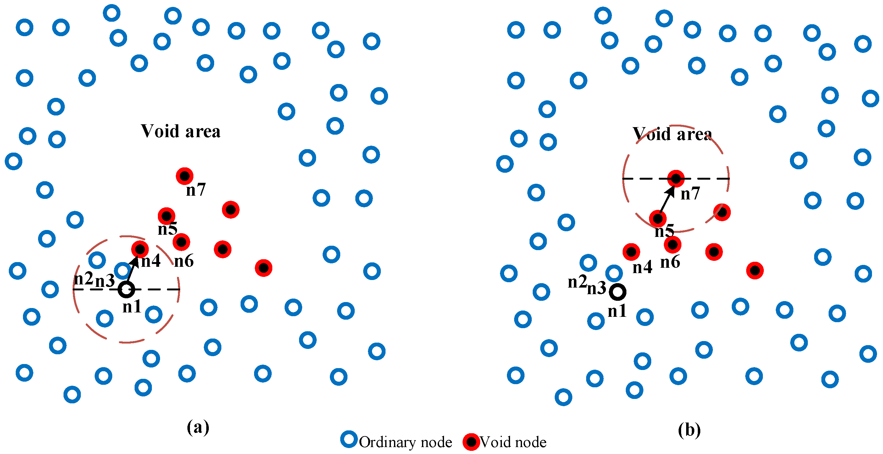
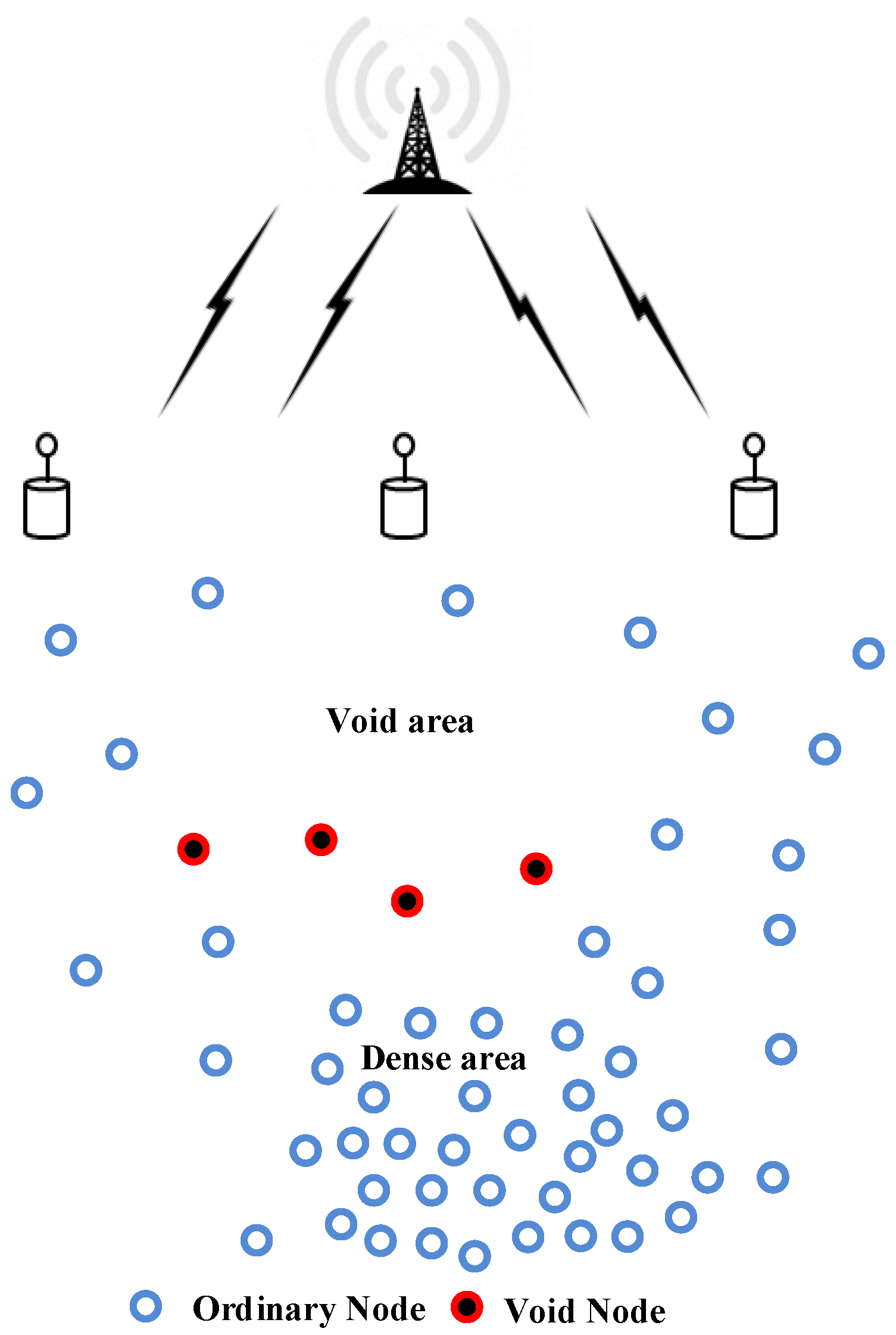
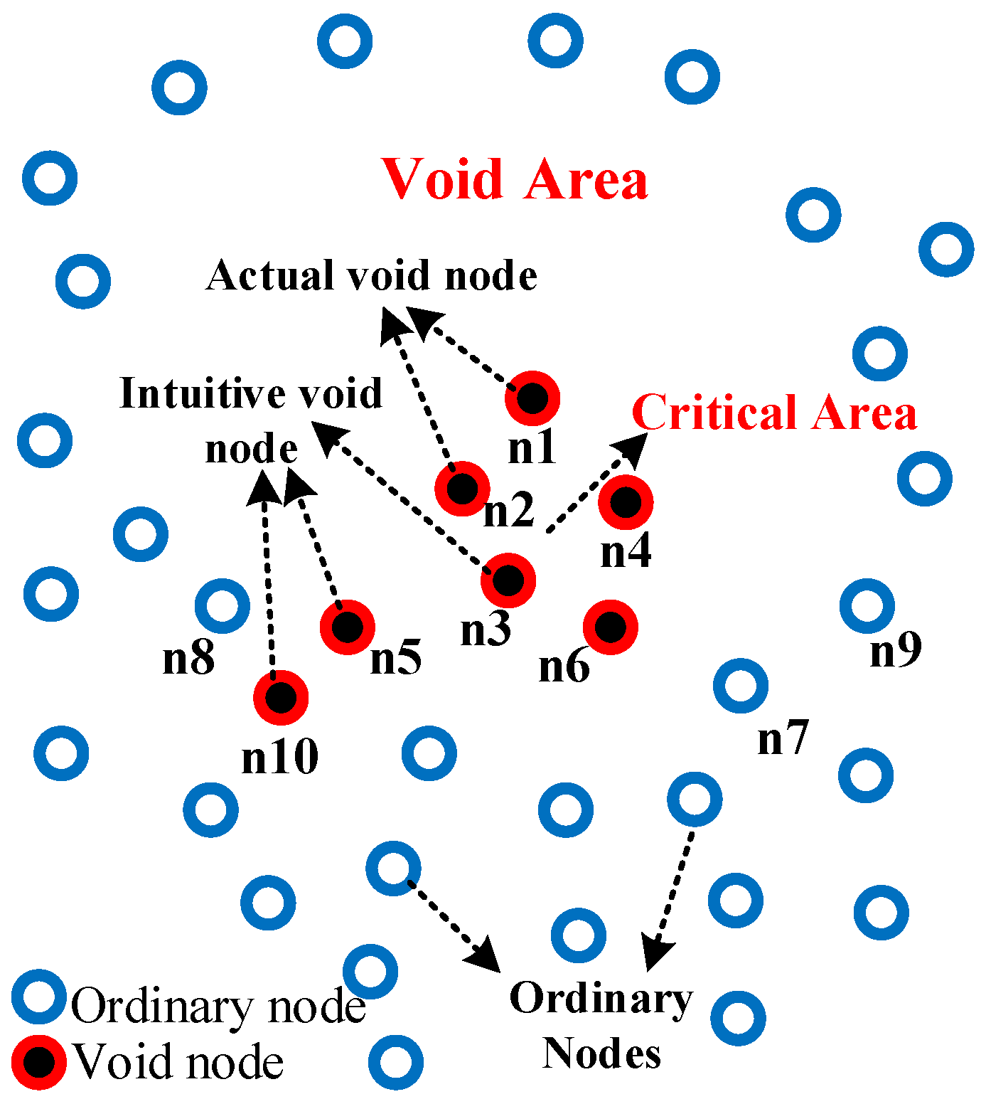
- Void area: the area without any sensors.
- Actual void node: the node that without shallower candidate set in its Routing Table (RT).
- Intuitive void node: the node can be considered as an intuitive void node in two scenarios:
- d.
- Critical area: the area that contains the actual void node, intuitive void node, or both.
- e.
- Void node: the node could be identified as a void node if it is an actual or intuitive void node.
3.3. Overview of EVA
3.4. An Efficient Void Aware Routing Protocol: Design Approach
3.4.1. EVA: Tables and Packets Format
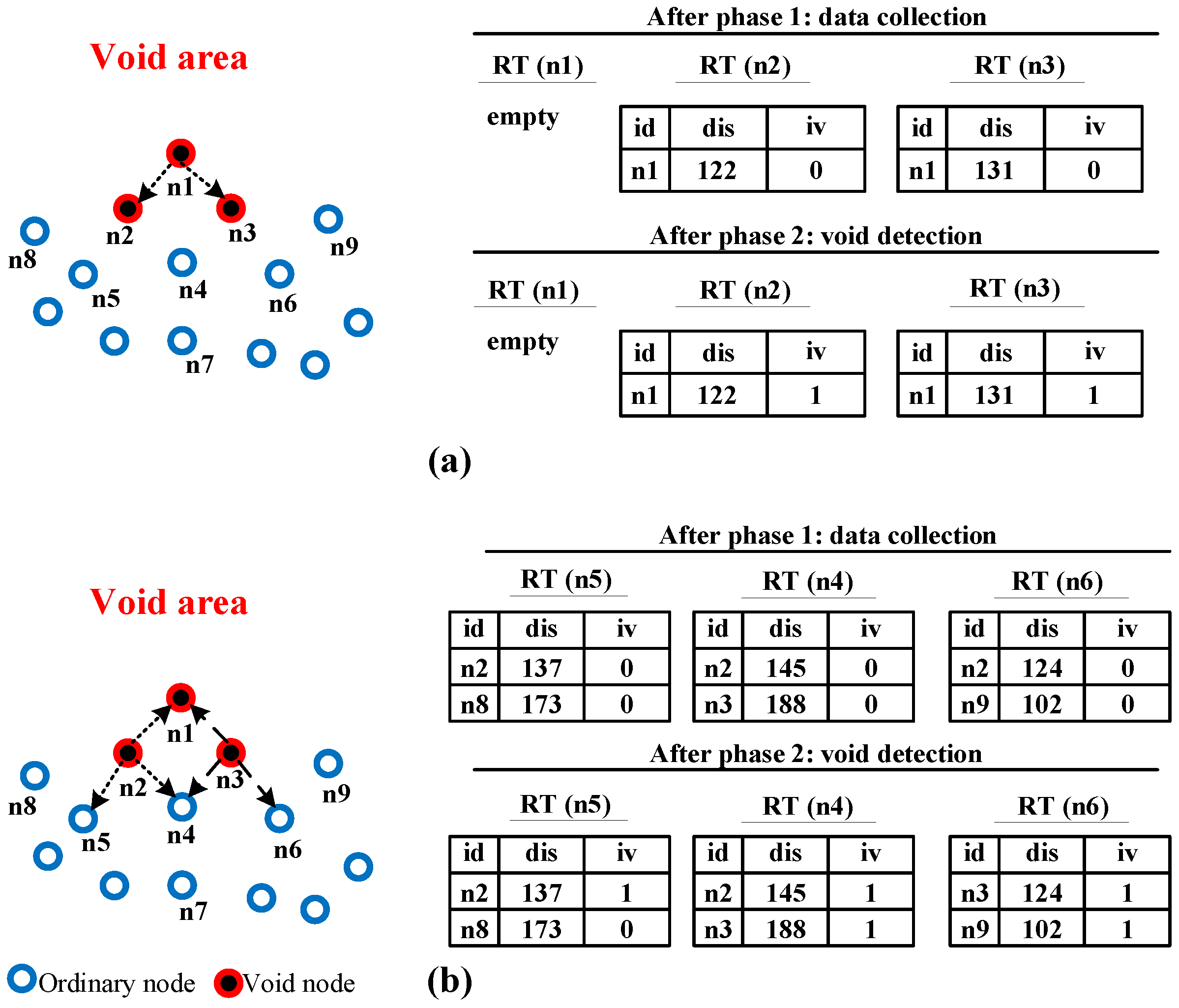
3.4.2. Data Collection Phase
3.4.3. Void Detection Phase
| Algorithm 1: EVA: Void Detection Algorithm. | |
| 1. | procedure . () |
| 2. | if then |
| 3. | if then |
| 4. | Generate () |
| 5. | |
| 6. | |
| 7. | |
| 8. | end if |
| 9. | end if |
| 10. | end procedure |
| 11. | procedure () |
| 12. | if ( then |
| 13. | return |
| 14. | else |
| 15. | |
| 16. | |
| 17. | end if |
| 18. | |
| 19. | |
| 20. | for to do |
| 21. | if () then |
| 22. | |
| 23. | Else |
| 24. | |
| 25. | end if |
| 26. | end for |
| 27. | if () then |
| 28. | |
| 29. | |
| 30. | |
| 31. | else if () then |
| 32. | Let |
| 33. | Let |
| 34. | for to do |
| 35. | if () & () then |
| 36. | |
| 37. | end if |
| 38. | end for |
| 39. | if () then |
| 40. | |
| 41. | . |
| 42. | Broadcast |
| 43. | end if |
| 44. | else |
| 45. | free () |
| 46. | end if |
| 47. | end procedure |
3.4.4. Data Forwarding Phase
| Algorithm 2: EVA: Efficient Void Aware Data Forwarding. | ||||
| 1: | procedure () | |||
| 2: | ||||
| 3: | while | |||
| 4: | ||||
| 5: | if () and () then | |||
| 6: | ||||
| 7: | ||||
| 8: | end if | |||
| 9: | ||||
| 10: | end while | |||
| 11: | end procedure | |||
| 12: | ||||
| 13: | methodEVA-DF () | |||
| 14: | Sort based on in ascending order | |||
| 15: | Let | |||
| 16: | Let | |||
| 17: | for to do | |||
| 18: | if () then | |||
| 19: | ||||
| 20: | end if | |||
| 21: | end for | |||
| 22: | if () then | |||
| 23: | ||||
| 24: | else | |||
| 25: | if then | |||
| 26: | ||||
| 27: | end if | |||
| 28: | end if | |||
| 29: | Clear () | |||
| 30: | Let | |||
| 31: | if then | |||
| 32: | () | |||
| 33: | end if | |||
| 34: | if then | |||
| 35: | () | |||
| 36: | end if | |||
| 37: | if then | |||
| 38: | () | |||
| 39: | end if | |||
| 40: | return | |||
| 41: | end method | |||
4. Results and Discussion
4.1. Simulation Setting
4.2. Performance Metrics
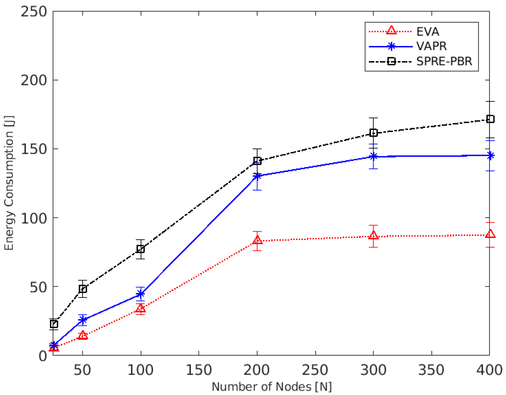
- Energy Consumption: the amount of energy consumed for each sensor.
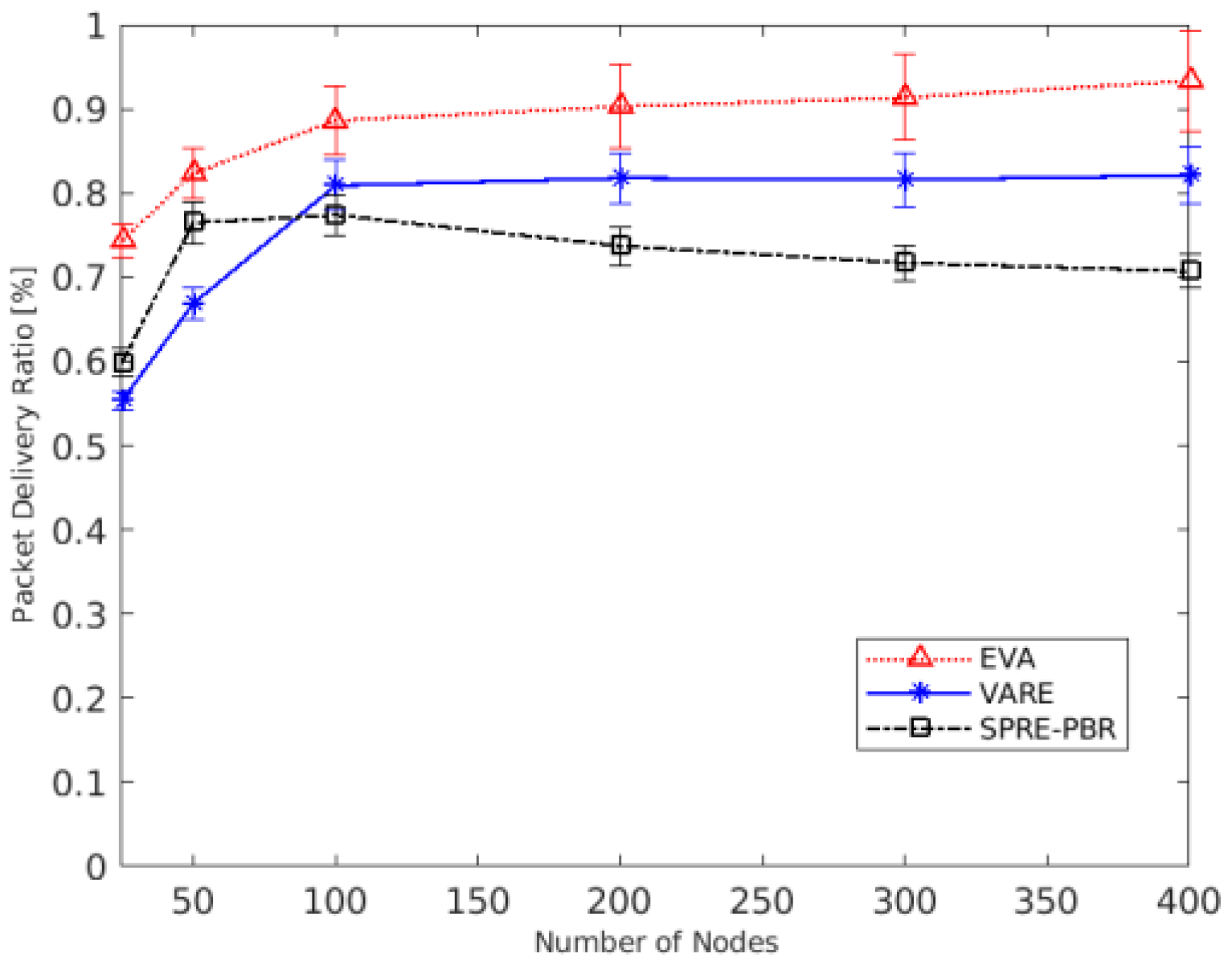
- Packet Delivery Ratio: the ratio of the successfully delivered packets to the sink divided by the number of total transmitted packets by each sensor.
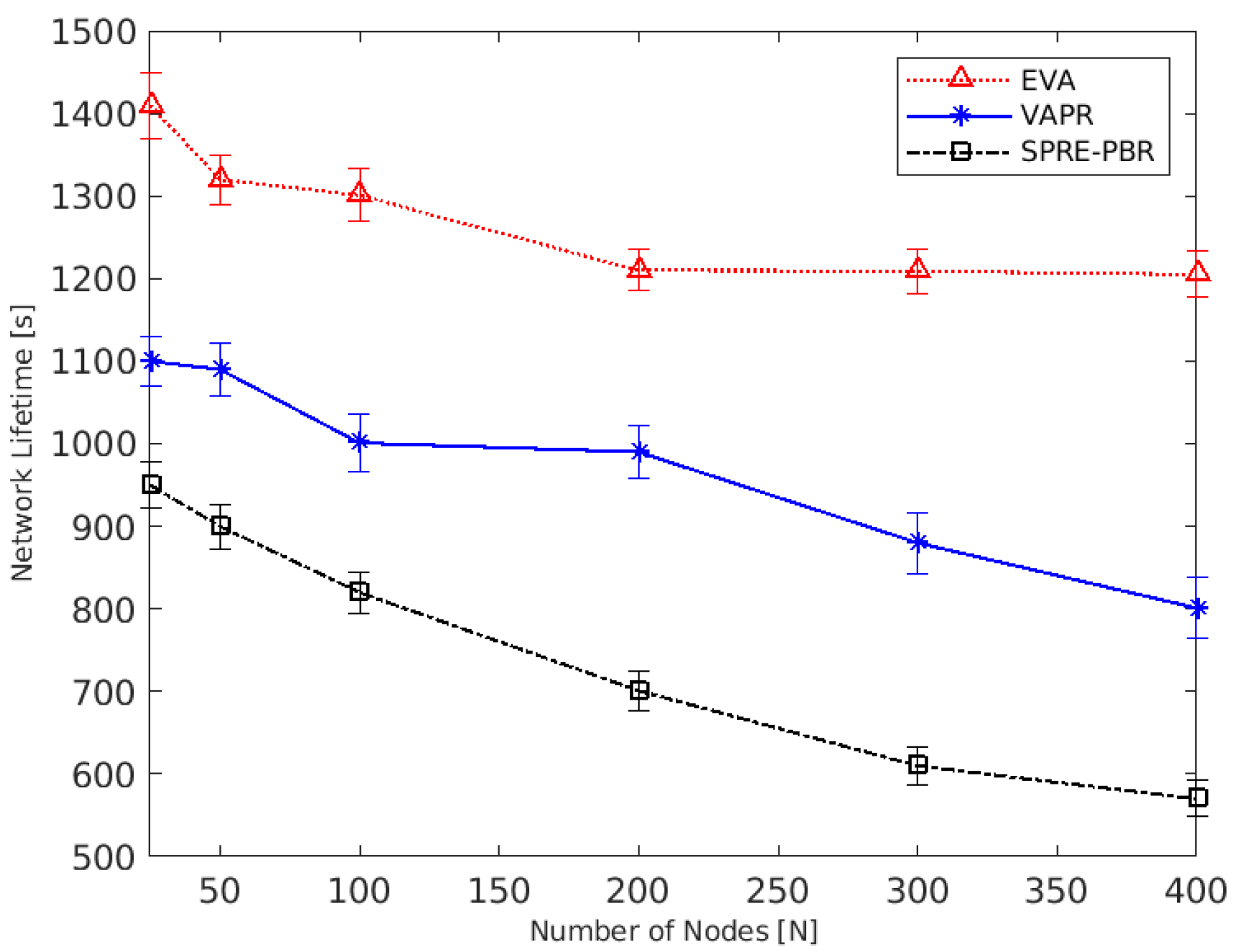
- Network Lifetime: the major lifetime that has been measured based on the first die sensor in the network.
- End-to-End Delay: the average delay caused by each sensor during the forwarding process.
4.3. Analysis of Results
5. Conclusions and Future Work
Author Contributions
Funding
Institutional Review Board Statement
Informed Consent Statement
Data Availability Statement
Conflicts of Interest
References
- Ayaz, M.; Baig, I.; Abdullah, A.; Faye, I. A survey on routing techniques in underwater wireless sensor networks. J. Netw. Comput. Appl. 2011, 34, 1908–1927. [Google Scholar] [CrossRef]
- Domingo, M.C. An overview of the internet of underwater things. J. Netw. Comput. Appl. 2012, 35, 1879–1890. [Google Scholar] [CrossRef]
- Kao, C.-C.; Lin, Y.-S.; Wu, G.-D.; Huang, C.-J. A Comprehensive Study on the Internet of Underwater Things: Applications, Challenges, and Channel Models. Sensors 2017, 17, 1477. [Google Scholar] [CrossRef] [Green Version]
- Kumar, V.; Kumar, S.; AlShboul, R.; Aggarwal, G.; Kaiwartya, O.; Khasawneh, A.; Lloret, J.; Al-Khasawneh, M. Grouping and Sponsoring Centric Green Coverage Model for Internet of Things. Sensors 2021, 21, 3948. [Google Scholar] [CrossRef]
- Liou, E.-C.; Kao, C.-C.; Chang, C.-H.; Lin, Y.-S.; Huang, C.-J. Internet of underwater things: Challenges and routing protocols. In Proceedings of the 2018 IEEE International Conference on Applied System Invention (ICASI), Chiba, Japan, 13–17 April 2018; pp. 1171–1174. [Google Scholar]
- Jouhari, M.; Ibrahimi, K.; Tembine, H.; Ben-Othman, J. Underwater Wireless Sensor Networks: A Survey on Enabling Technologies, Localization Protocols, and Internet of Underwater Things. IEEE Access 2019, 7, 96879–96899. [Google Scholar] [CrossRef]
- Song, Y. Underwater Acoustic Sensor Networks with Cost Efficiency for Internet of Underwater Things. IEEE Trans. Ind. Electron. 2020, 68, 1707–1716. [Google Scholar] [CrossRef]
- Khalifeh, A.; Darabkh, K.A.; Khasawneh, A.M.; Alqaisieh, I.; Salameh, M.; Alabdala, A.; Alrubaye, S.; Alassaf, A.; Al-Hajali, S.; Al-Wardat, R.; et al. Wireless Sensor Networks for Smart Cities: Network Design, Implementation and Performance Evaluation. Electronics 2021, 10, 218. [Google Scholar] [CrossRef]
- Zhou, Z.; Yao, B.; Xing, R.; Shu, L.; Bu, S. E-CARP: An Energy Efficient Routing Protocol for UWSNs in the Internet of Underwater Things. IEEE Sens. J. 2015, 16, 4072–4082. [Google Scholar] [CrossRef]
- Coutinho, R.W.L.; Boukerche, A.; Loureiro, A.A. A novel opportunistic power controlled routing protocol for internet of underwater things. Comput. Commun. 2019, 150, 72–82. [Google Scholar] [CrossRef]
- Khasawneh, A.; Latiff, M.S.B.A.; Kaiwartya, O.; Chizari, H. A reliable energy-efficient pressure-based routing protocol for underwater wireless sensor network. Wirel. Netw. 2018, 24, 2061–2075. [Google Scholar] [CrossRef]
- Mhemed, R.; Comeau, F.; Phillips, W.; Aslam, N. Void Avoidance Opportunistic Routing Protocol for Underwater Wireless Sensor Networks. Sensors 2021, 21, 1942. [Google Scholar] [CrossRef]
- Khasawneh, A.; Latiff, M.S.B.A.; Kaiwartya, O.; Chizari, H. Next Forwarding Node Selection in Underwater Wireless Sensor Networks (UWSNs): Techniques and Challenges. Information 2017, 8, 3. [Google Scholar] [CrossRef] [Green Version]
- Khasawneh, A.M.; Kaiwartya, O.; Lloret, J.; Abuaddous, H.Y.; Abualigah, L.; Al Shinwan, M.; Al-Khasawneh, M.A.; Mahmoud, M.; Kharel, R. Green Communication for Underwater Wireless Sensor Networks: Triangle Metric Based Multi-Layered Routing Protocol. Sensors 2020, 20, 7278. [Google Scholar] [CrossRef]
- Alfouzan, F.; Shahrabi, A.; Ghoreyshi, S.M.; Boutaleb, T. A Comparative Performance Evaluation of Distributed Collision-free MAC Protocols for Underwater Sensor Networks. In Proceedings of the 8th International Conference on Sensor Networks, Prague, Czech Republic, 26–27 February 2019; pp. 85–93. [Google Scholar] [CrossRef]
- Khasawneh, A.M.; Abualigah, L.; Al Shinwan, M. Void Aware Routing Protocols in Underwater Wireless Sensor Networks: Variants and challenges. J. Phys. Conf. Ser. 2020, 1550, 032145. [Google Scholar] [CrossRef]
- Khasawneh, A.M.; Kaiwartya, O.; Khalifeh, A.; Abualigah, L.M.; Lloret, J. Green Computing in Underwater Wireless Sensor Networks Pressure Centric Energy Modeling. IEEE Syst. J. 2020, 14, 4735–4745. [Google Scholar] [CrossRef]
- Khasawneh, A.; Bin Abd Latiff, M.S.; Chizari, H.; Tariq, M.; Bamatraf, A. Pressure based routing protocol for underwater wireless sensor networks: A survey. KSII Trans. Internet Inf. Syst. (TIIS) 2015, 9, 504–527. [Google Scholar] [CrossRef]
- Rehman, Z.U.; Iqbal, A.; Yang, B.; Hussain, T. Void Hole Avoidance Based on Sink Mobility and Adaptive Two Hop Vector-Based Forwarding in Underwater Wireless Sensor Networks. Wirel. Pers. Commun. 2021, 120, 1417–1447. [Google Scholar] [CrossRef]
- Alfouzan, F.A.; Shahrabi, A.; Ghoreyshi, S.M.; Boutaleb, T. A Collision-Free Graph Coloring MAC Protocol for Underwater Sensor Networks. IEEE Access 2019, 7, 39862–39878. [Google Scholar] [CrossRef]
- Kanthimathi, N. Void handling using Geo-Opportunistic Routing in underwater wireless sensor networks. Comput. Electr. Eng. 2017, 64, 365–379. [Google Scholar] [CrossRef]
- Xie, P.; Zhou, Z.; Peng, Z.; Cui, J.-H.; Shi, Z. Void Avoidance in Three-Dimensional Mobile Underwater Sensor Networks. In Proceedings of the International Conference on Wireless Algorithms, Honolulu, HI, USA, 24–26 June 2009; pp. 305–314. [Google Scholar] [CrossRef]
- Noh, Y.; Lee, U.; Wang, P.; Choi, B.S.C.; Gerla, M. VAPR: Void-Aware Pressure Routing for Underwater Sensor Networks. IEEE Trans. Mob. Comput. 2012, 12, 895–908. [Google Scholar] [CrossRef]
- Ghoreyshi, S.M.; Shahrabi, A.; Boutaleb, T. An inherently void avoidance routing protocol for underwater sensor networks. In Proceedings of the 2015 International Symposium on wireless communication systems (ISWCS), Brussels, Belgium, 25–28 August 2015; pp. 361–365. [Google Scholar]
- Sher, A.; Khan, A.; Javaid, N.; Ahmed, S.H.; Aalsalem, M.Y.; Khan, W.Z. Void Hole Avoidance for Reliable Data Delivery in IoT Enabled Underwater Wireless Sensor Networks. Sensors 2018, 18, 3271. [Google Scholar] [CrossRef] [Green Version]
- Alfouzan, F. Energy-Efficient Collision Avoidance MAC Protocols for Underwater Sensor Networks: Survey and Challenges. J. Mar. Sci. Eng. 2021, 9, 741. [Google Scholar] [CrossRef]
- Al-Shalabi, M.; Anbar, M.; Wan, T.-C.; Khasawneh, A. Variants of the Low-Energy Adaptive Clustering Hierarchy Protocol: Survey, Issues and Challenges. Electronics 2018, 7, 136. [Google Scholar] [CrossRef] [Green Version]
- Ibrahim, D.M.; Eltobely, T.E.; Fahmy, M.M.; Sallam, E.A. Enhancing the vector-based forwarding routing protocol for underwater wireless sensor networks: A clustering approach. In Proceedings of the International Conference on Wireless and Mobile Communications, Seville, Spain, 22–26 June 2014; pp. 98–104. [Google Scholar]
- Hwang, D.; Kim, D. DFR: Directional flooding-based routing protocol for underwater sensor networks. In Proceedings of the OCEANS 2008, Quebec City, QC, Canada, 15–18 September 2008; pp. 1–7. [Google Scholar] [CrossRef]
- Jornet, J.M.; Stojanovic, M.; Zorzi, M. Focused beam routing protocol for underwater acoustic networks. In Proceedings of the Third ACM International Workshop on Underwater Networks, San Francisco, CA, USA, 15 September 2008; pp. 75–82. [Google Scholar]
- Wahid, A.; Lee, S.; Kim, D.; Lim, K.-S. MRP: A Localization-Free Multi-Layered Routing Protocol for Underwater Wireless Sensor Networks. Wirel. Pers. Commun. 2014, 77, 2997–3012. [Google Scholar] [CrossRef]
- Al Bzoor, M.; Zhu, Y.; Liu, J.; Ammar, R.; Cui, J.H.; Rajasekaran, S. An adaptive power controlled routing protocol for underwater sensor network. Int. J. Sens. Netw. 2015, 18, 238. [Google Scholar] [CrossRef]
- Noh, Y.; Lee, U.; Lee, S.; Wang, P.; Vieira, L.F.M.; Cui, J.-H.; Gerla, M.; Kim, K. HydroCast: Pressure Routing for Underwater Sensor Networks. IEEE Trans. Veh. Technol. 2015, 65, 333–347. [Google Scholar] [CrossRef]
- Ganesh, N. Performance Evaluation of Depth Adjustment and Void Aware Pressure Routing (DA-VAPR) Protocol for Underwater Wireless Sensor Networks. Comput. J. 2019, 63, 193–202. [Google Scholar] [CrossRef]
- Ghoreyshi, S.M.; Shahrabi, A.; Boutaleb, T. An opportunistic void avoidance routing protocol for underwater sensor networks. In Proceedings of the 2016 IEEE 30th International Conference on Advanced Information Networking and Applications (AINA), Crans-Montana, Switzerland, 23–25 March 2016; pp. 316–323. [Google Scholar]
- Yan, H.; Shi, Z.J.; Cui, J.-H. DBR: Depth-based routing for underwater sensor networks. In Proceedings of the International Conference on Research in Networking, Singapore, 5–9 May 2008; pp. 72–86. [Google Scholar]
- Wahid, A.; Kim, D. An Energy Efficient Localization-Free Routing Protocol for Underwater Wireless Sensor Networks. Int. J. Distrib. Sens. Netw. 2012, 8, 307246. [Google Scholar] [CrossRef]
- Jafri, M.; Ahmed, S.; Javaid, N.; Ahmad, Z.; Qureshi, R. AMCTD: Adaptive Mobility of Courier Nodes in Threshold-Optimized DBR Protocol for Underwater Wireless Sensor Networks. In Proceedings of the 2013 Eighth International Conference on Broadband and Wireless Computing, Communication and Applications, Washington, DC, USA, 28–30 October 2013; pp. 93–99. [Google Scholar] [CrossRef] [Green Version]
- Xie, P.; Zhou, Z.; Peng, Z.; Yan, H.; Hu, T.; Cui, J.-H.; Shi, Z.; Fei, Y.; Zhou, S. Aqua-Sim: An NS-2 based simulator for underwater sensor networks. In Proceedings of the OCEANS 2009, Biloxi, MS, USA, 26–29 October 2009. [Google Scholar] [CrossRef]
- Mirza, D.; Lu, F.; Schurgers, C. Efficient broadcast MAC for underwater networks. In Proceedings of the Fourth ACM International Workshop on UnderWater Networks (WUWNet), Berkeley, CA, USA, 3 November 2009. [Google Scholar]


| Symbol | Description | Symbol | Description |
|---|---|---|---|
| -th sensor Nodes | Void Count Sensors in RT | ||
| Sensor node ID | Ordinary count sensors in RT | ||
| RT | Routing Table | The reliable value in RT | |
| Candidate set in RT | Reliable status = “Very good link” | ||
| void probe packet | The number of “Very good link” in RT | ||
| Boolean Value (True or False) | Sender node ID | ||
| loc | The location of the sensor in the RT | Retransmission time | |
| Void status in the RT |
| Symbol | Description | Symbol | Description |
|---|---|---|---|
| Transmission Range | Void count sensors in RT | ||
| Candidate set in NIT | -th sensor nodes, | ||
| Best neighbors | Routing Table | ||
| EN | The number of eligible sensors in EVA-DF | Sensor node ID | |
| Depth differences between sender and receiver | Set of ordinary neighbors in EVA-DF | ||
| Depth value | The route cost field in the data packet | ||
| Void status in the RT | The highest number of the best candidate set |
| Simulation Parameter | Values |
|---|---|
| Number of sensor nodes | 50–400 |
| Network topology | Random topology |
| Deployment area | |
| Bandwidth | |
| Communication medium | Acoustic Waves |
| Area of transmission range | m |
| MAC protocol | |
| Node movement | 0–3 |
| Hello packet interval | |
| Data packet size | bytes |
| Initial energy | |
| Power consumption | |
| Packet generation time | |
| Number of Runs | 50 |
| % Improvements of EVA as Compared with Existing Techniques | ||||||
|---|---|---|---|---|---|---|
| Nodes | VAPR | SPRE-PBR | EVA | % Improvement of EVA as Compared with SPRE-PBR | % Improvement of EVA as Compared with VAPR | |
| Node vs. Energy Consumption (J) | 25 | 7.2987 | 22.5984 | 5.3852 | 76.1699943 | 26.2169975 |
| 50 | 25.6574 | 48.3955 | 13.9745 | 71.1243814 | 45.5342318 | |
| 100 | 44.4363 | 77.1954 | 33.8731 | 56.1203129 | 23.7715561 | |
| 200 | 140.2047 | 141.1042 | 83.1745 | 41.054554 | 40.6763825 | |
| 300 | 144.3546 | 161.2050 | 86.4730 | 46.3583636 | 40.0968171 | |
| 400 | 145.1486 | 171.1740 | 87.4040 | 48.938507 | 39.7830913 | |
| Average % Improvements | 56.6276855 ↓ | 36.0131794 ↓ | ||||
| Node vs. Packet Delivery Ratio (%) | 25 | 0.5531 | 0.5981 | 0.7429 | 24.21 | 34.3156753 |
| 50 | 0.6684 | 0.7647 | 0.8233 | 7.663136 | 23.1747457 | |
| 100 | 0.8088 | 0.7739 | 0.8862 | 14.51092 | 9.56973294 | |
| 200 | 0.8177 | 0.7371 | 0.9027 | 22.46642 | 10.3950104 | |
| 300 | 0.8155 | 0.7171 | 0.9135 | 27.38809 | 12.0171674 | |
| 400 | 0.8211 | 0.7072 | 0.9333 | 31.97115 | 13.6645963 | |
| Average % Improvements | 21.36829 ↑ | 17.189488 ↑ | ||||
| Node vs. Network Lifetime (Sec) | 25 | 1100 | 950 | 1410 | 48.42105 | 28.1818182 |
| 50 | 1090 | 900 | 1320 | 46.66667 | 21.1009174 | |
| 100 | 1001 | 820 | 1301 | 58.65854 | 29.97003 | |
| 200 | 990 | 701 | 1210 | 72.61056 | 22.2222222 | |
| 300 | 880 | 610 | 1209 | 98.19672 | 37.3863636 | |
| 400 | 801 | 570 | 1205 | 111.4035 | 50.4369538 | |
| Average % Improvements | 72.65951 ↑ | 31.5497175 ↑ | ||||
| Node vs. End-to-End Delay (ms) | 25 | 13.9620 | 17.6721 | 9.0468 | 48.80744 | 35.2041255 |
| 50 | 14.3984 | 23.7532 | 10.1746 | 57.16535 | 29.3352039 | |
| 100 | 18.2798 | 33.1678 | 11.1706 | 66.32095 | 38.8910163 | |
| 200 | 27.0748 | 35.1045 | 12.7658 | 63.63486 | 52.8498825 | |
| 300 | 36.5000 | 49.1000 | 13.4010 | 72.70672 | 63.2849315 | |
| 400 | 41.4862 | 51.3475 | 14.2354 | 72.27635 | 65.686421 | |
| Average % Improvements | 63.48528 ↓ | 47.5419301 ↓ | ||||
Publisher’s Note: MDPI stays neutral with regard to jurisdictional claims in published maps and institutional affiliations. |
© 2021 by the authors. Licensee MDPI, Basel, Switzerland. This article is an open access article distributed under the terms and conditions of the Creative Commons Attribution (CC BY) license (https://creativecommons.org/licenses/by/4.0/).
Share and Cite
Khasawneh, A.M.; Altalhi, M.; Kumar, A.; Aggarwal, G.; Kaiwartya, O.; Khalifeh, A.; Al-Khasawneh, M.A.; Alarood, A.A. An Efficient Void Aware Framework for Enabling Internet of Underwater Things. J. Mar. Sci. Eng. 2021, 9, 1219. https://doi.org/10.3390/jmse9111219
Khasawneh AM, Altalhi M, Kumar A, Aggarwal G, Kaiwartya O, Khalifeh A, Al-Khasawneh MA, Alarood AA. An Efficient Void Aware Framework for Enabling Internet of Underwater Things. Journal of Marine Science and Engineering. 2021; 9(11):1219. https://doi.org/10.3390/jmse9111219
Chicago/Turabian StyleKhasawneh, Ahmad M., Maryam Altalhi, Arvind Kumar, Geetika Aggarwal, Omprakash Kaiwartya, Ala’ Khalifeh, Mahmoud Ahmad Al-Khasawneh, and Ala Abdulsalam Alarood. 2021. "An Efficient Void Aware Framework for Enabling Internet of Underwater Things" Journal of Marine Science and Engineering 9, no. 11: 1219. https://doi.org/10.3390/jmse9111219
APA StyleKhasawneh, A. M., Altalhi, M., Kumar, A., Aggarwal, G., Kaiwartya, O., Khalifeh, A., Al-Khasawneh, M. A., & Alarood, A. A. (2021). An Efficient Void Aware Framework for Enabling Internet of Underwater Things. Journal of Marine Science and Engineering, 9(11), 1219. https://doi.org/10.3390/jmse9111219