Numerical Simulation of Sediment Plume Dispersion in Deep-Sea Mining Areas Based on the Similarity Principle

Abstract

Sediment plumes generated by seafloor mining vehicles represent a major environmental concern in polymetallic nodule harvesting operations. This study investigates plume dispersion induced by sediment disturbances during mining using numerical simulations based on the similarity principle. A representative mining region is modeled, and the motion of mining vehicles is simulated to define the sediment disturbance source. The simulations employ the experimentally validated P-T Euler model (Particle–Turbulence Interaction Euler model) to examine the effects of sediment release velocity and ambient current velocity on plume dispersion characteristics. The results show that increasing the sediment release velocity primarily enhances the initial turbidity flux and significantly expands the plume core diffusion range, indicating that mining disturbances dominate near-field plume behavior. In contrast, the ambient current velocity strongly controls plume morphology and transport, promoting upward transport, long-range advection, and enhanced turbulent dissipation that governs far-field dispersion. Overall, plume diffusion is initially controlled by mining-induced sediment release but becomes increasingly dominated by ambient flow during large-scale transport. These findings provide a theoretical basis for predicting sediment plume behavior and assessing potential environmental impacts in deep-sea mining areas.

1. Introduction

Deep-sea mining has emerged as a promising approach for exploiting polymetallic nodules and other seabed mineral resources to meet the growing global demand for critical metals. These resources, which contain critical metals such as nickel, cobalt, and copper, play an indispensable role in ensuring national resource security and supporting sustainable economic development [1,2,3]. Among these, polymetallic nodules have become a primary research focus in the field of deep-sea mining due to their abundant critical metal content and occurrence form favorable for extraction; therefore, in the following discussion, the issue of polymetallic nodule collection will be taken as an example to carry out the relevant research. However, mining activities inevitably disturb seafloor sediments, generating suspended sediment plumes that can spread over large areas and potentially affect deep-sea ecosystems. These sediment plumes are typically produced by the mechanical disturbance of seabed materials by mining vehicles and associated equipment, resulting in complex interactions between sediment particles and ambient ocean currents [4]. This issue is particularly concerning due to its profound impact on benthic habitats and the broader marine ecological chain [5,6,7]. Understanding the generation, transport, and dispersion mechanisms of such plumes is therefore essential for evaluating the environmental impacts of deep-sea mining operations and for developing effective mitigation strategies. Numerical modeling has become an important tool for investigating plume dynamics, as it allows the systematic analysis of the key physical processes governing sediment transport under various operational and environmental conditions.

The dispersion of sediment plumes generated during deep-sea mining results from complex interactions among seawater, sediment particles, and near-bed ocean currents. Early investigations by Ouillon et al. [8] examined plume behavior induced by mining vehicle operations and identified a negative correlation between the morphology of the gravity-current front and the ratio of mining vehicle velocity to particle settling velocity. Building on this work, they proposed a simplified advection–diffusion–settling model capable of predicting tailings plume transport, which demonstrated a good predictive capability for plume behavior during deep-sea mining operations [9]. Liu et al. [10,11] subsequently used an Euler–Lagrange framework combined with laboratory experiments to investigate the wake structures of mining vehicles and their influence on plume entrainment and wrapping. They proposed a three-stage evolution mechanism considering inertial forces, negative buoyancy, and near-bed recovery processes. The Liu-Ganghui team [12] applied the Euler two-fluid model in numerical simulations to examine fine particle plume diffusion during deep-sea mining. Their analysis focused on how initial discharge mass concentration and discharge velocity influenced the plume’s evolution and development near the seabed. Studies by Yang et al. [13] and Bai et al. [14] applied coupled Discrete Element Method–Large Eddy Simulation (DEM–LES) and Reynolds-Averaged Navier–Stokes (RANS) models to investigate the effects of discharge velocity, particle concentration, pipeline diameter, and particle size on plume evolution.

Experimental investigations have further advanced the understanding of plume formation and sediment transport. Decrop et al. [15] developed an experimental method using an Acoustic Doppler Velocimeter (ADV) to measure turbulent momentum and sediment fluxes, validating a fine-particle plume model simulating tailings discharge. In laboratory tank experiments, Byishimo [16] studied the formation, dispersion, and deposition of mining tailings plumes, showing that lower injection heights produced more confined plume dispersion and that lower sediment concentrations reduced post-settling accumulation. The group at the Delft University of Technology, led by Wijmans [17], systematically investigated the influence of initial sediment concentration on turbidity current propagation, demonstrating its critical role in plume transport and spatial diffusion. Field-based studies have provided essential validation and insights into real-world plume behavior. Liu et al. [18] developed coupled far-field numerical models to analyze plume dispersion under varying ratios of tailings discharge velocity to mining vehicle speed, finding that higher relative discharge velocities enhanced sediment settling while expanding horizontal diffusion. Purkiani et al. [19] established and validated a numerical framework through experiments. Based on this validated numerical framework, they comprehensively considered multiple factors, including sediment characteristics and marine hydrodynamic conditions, to achieve an optimal statistical fit between sensor-based observations and model outputs. The results showed that the model was capable of reproducing the observed suspended sediment concentrations and redeposition patterns during the dredging experiment. In situ measurements in regions such as the Clarion–Clipperton Zone indicate that high suspended sediment concentrations can suppress vertical mixing, confining plume diffusion to approximately 2 m above the seabed and highlighting the controlling influence of turbulence intensity [20,21]. Additionally, field experiments by Spearman et al. [22] showed that plume dispersion was strongly influenced by particle flocculation, background turbidity, and near-bed currents.

Despite these advances, existing studies have primarily addressed isolated aspects of plume dynamics, such as vehicle wake effects, tailings discharge behavior, or regional hydrodynamic transport. Systematic investigations that integrate mining vehicle disturbances, seabed hydrodynamic conditions, and sediment transport processes within a unified simulation and experimental framework remain limited. Addressing this gap is essential for improving the reliability of plume dispersion predictions and supporting environmental impact assessments in future deep-sea mining operations. This study therefore employs a comprehensive numerical simulation framework to evaluate sediment plume transport under realistic mining scenarios, accounting for key factors including bottom currents, vehicle-induced disturbances, and discharge characteristics.

In summary, although extensive data have been obtained from theoretical analyses, numerical simulations, and experimental investigations and provided important support for the potential commercialization of deep-sea mining, the spatial extent and environmental impact of mining-induced sediment plumes remain difficult to quantify with confidence. This uncertainty has contributed to ambiguities in regulatory frameworks, thereby constraining the progress of deep-sea mining commercialization. Consequently, systematic research and integrated evaluation of plume dispersion from a holistic perspective of seabed mining operations are urgently required.

Building on previous studies and applying the principle of similarity, this study simulates realistic mining operation scenarios while incorporating key environmental factors such as bottom currents. A numerical simulation framework is employed to assess the dispersion of sediment plumes during deep-sea mining operations, focusing on the effects of mining vehicle disturbance and ambient hydrodynamic conditions on the transport, as well as the dispersion of the plume within both near-field and far-field extents. In this study, the far field is defined as the region extending up to approximately 13 times the mining site area (i.e., beyond the immediate near-field zone where mining-induced disturbances dominate).

2. Numerical Methods

2.1. Mathematical Model

The dispersion of plumes during deep-sea mining involves the mutual mixing motion between sediment particles and the surrounding fluid, making it a typical two-phase flow problem involving solids and liquids. Currently, three main numerical methods are used to simulate this phenomenon: (1) simplified models for high-density gravity currents [8], which ignore the interactions between particles and fluids and thus offer a lower accuracy; (2) fluid–particle coupling models [13,23], which independently calculate the particle and fluid phases, providing a high accuracy but requiring substantial computational resources; and (3) Euler–Euler models [24,25,26], which treat the particle phase as a pseudo-fluid and account for both particle–particle and particle–fluid interactions, maintaining a high accuracy while reducing computational costs and making them suitable for engineering applications.

Considering the advantages and disadvantages of the methods discussed above, this paper adopts the Euler–Euler model in conjunction with particle kinetic theory, focusing on the interactions between particles–particles and particles–fluid. When simulating the flow characteristics of fine-grained solid–liquid two-phase flow, we will introduce correction terms into the Navier–Stokes (N-S) equations to enhance the accuracy of the simulation.

The characteristic of the Euler–Euler model lies in treating the solid and liquid phases as mutually permeable media, while introducing the concept of a phase volume fraction to represent the proportion of each phase occupying the volume in the space [27].

$$V_q={\displaystyle \int {\alpha }_q}dV$$

(1)

where V_q presents the volume of phase q; α_q represents the volume fraction; and q is f for the liquid phase and s for the solid phase, with ${\alpha }_f+{\alpha }_s=1$.

(1)

Correction of the momentum conservation equation

The momentum conservation equation for the solid–liquid two-phase flow can be expressed as:

$${\displaystyle \frac{\partial }{\partial t}}({\alpha }_q{\rho }_q{\overrightarrow{v}}_q)+\nabla \cdot ({\alpha }_q{\rho }_q{\overrightarrow{v}}_q{\overrightarrow{v}}_q)=-{\alpha }_q\nabla p-\nabla p_q+\nabla \cdot {\overline{\overline{\tau }}}_q+{\alpha }_q{\rho }_{q}g+F$$

(2)

where p represents the shared pressure of both phases; ρ represents the phase density; g denotes the gravitational acceleration; and ${\overline{\overline{\tau }}}_q$ is the stress–strain tensor for phase q, which can be expressed as:

$${\overline{\overline{\tau }}}_q={\alpha }_q{\mu }_q(\nabla {\overrightarrow{v}}_q+\nabla {\overrightarrow{v}}_q^T)+{\alpha }_q({\lambda }_q-{\displaystyle \frac{2}{4}}{\mu }_q)\nabla \cdot {\overrightarrow{v}}_q\overline{\overline{I}}$$

(3)

where ${\mu }_q$ and ${\lambda }_q$ represent the shear viscosity and volumetric viscosity of phase q, respectively; and $\overline{\overline{I}}$ denotes the unit tensor.

In Equation (2), F represents the various forces acting on the particles during the two-phase flow. These forces include the interphase interaction forces, external body forces, lift, wall lubrication forces, and virtual mass forces [28,29,30,31,32]. Within the two-phase flow field, the lift force increases with particle size. For smaller particles, however, the influence of lift is generally negligible. The wall lubrication force primarily affects the movement of bubbles near the wall, particularly in regions that are in close proximity to the wall. The virtual mass force, which results from the accelerated motion of the particles relative to the fluid, only becomes significant when the particle density is much smaller than that of the fluid [33,34].

This study focuses on micron-sized particles with a density of 2650 kg/m³, which are typical small-sized, high-density solid particles. Therefore, during the calculation process, the effects of lift, wall lubrication forces, and virtual mass forces can be neglected. This not only simplifies the calculation process but also saves computational resources while ensuring calculation accuracy. Hence, the expression for F can be represented as:

$$F=F_{inter}+F_q$$

(4)

where F_inter and F_q represent the interphase interaction force and the external body force, respectively.

The interphase interaction force between the solid and liquid phases in the above equation is represented in the solid phase momentum conservation law as:

$$F_{s-\mathrm{int}er}=K_{fs}({\overrightarrow{v}}_f-{\overrightarrow{v}}_s)$$

(5)

where $K_{sf}=K_{fs}$ represents the momentum exchange coefficient between the solid and liquid phases. Since the interaction between the solid and liquid phases satisfies Newton’s third law of motion, the interphase interaction force in the liquid phase is given by $F_{f-\mathrm{int}er}=-F_{s-\mathrm{int}er}$.

The general expression for $K_{sf}$ can be written as:

$$K_{sf}={\displaystyle \frac{{\alpha }_s{\rho }_{s}f}{{\tau }_s}}$$

(6)

where ${\rho }_s$ represents the solid phase density; f takes different values for different exchange coefficient models, which will be discussed in detail in the following sections; and ${\tau }_s$ represents the particle relaxation time, and its expression is given by:

$${\tau }_s={\displaystyle \frac{{\rho }_s{d}_s^2}{18{\mu }_f}}$$

(7)

where d_s represents the particle diameter; and ${\mu }_f$ represents the dynamic viscosity of the liquid phase.

In the study of solid–liquid two-phase flow, the Wen & Yu model is commonly adopted when the solid phase volume fraction is below 0.2 (the volume fraction used throughout this study). In this study, the solid phase volume fraction is set to 0.02, making the use of the Wen & Yu model for analysis highly appropriate. The model provides the expression for the momentum exchange coefficient between the solid and liquid phases as [35]:

$$K_{sf}={\displaystyle \frac{3}{4}}{C}_D{\displaystyle \frac{{\alpha }_s{\alpha }_f{\rho }_f\left|{\overrightarrow{v}}_s-{\overrightarrow{v}}_f\right|}{d_s}}{\alpha }_f^{-2.65}$$

(8)

$$C_D={\displaystyle \frac{24}{{\alpha }_f{\mathrm{Re}}_s}}[1+0.15{({\alpha }_f{\mathrm{Re}}_s)}^{0.687}]$$

(9)

$${\mathrm{Re}}_s={\displaystyle \frac{{\rho }_f{d}_s\left|{\overrightarrow{v}}_s-{\overrightarrow{v}}_f\right|}{{\mu }_f}}$$

(10)

where C_D represents the drag coefficient; and Re_s represents the relative Reynolds number.

The drag coefficient in the Wen & Yu model incorporates the effect of the phase volume fraction based on the standard drag model formula, but it does not consider the effect of turbulence on the drag coefficient. As a dilute-phase drag calculation model, the impact of turbulence intensity on the drag coefficient is generally more significant than the phase volume fraction [36]. According to experimental studies in the related literature [37,38,39], fluid turbulence intensity leads to an increase in the drag coefficient in solid–liquid two-phase flow; therefore, when applying the drag coefficient formula of the Wen & Yu model, it is necessary to modify the formula to account for the effect of turbulence on the drag force.

Brucato et al. [38] proposed a new experimental technique to measure the average particle drag coefficient in turbulent media, and obtained a relationship between the drag coefficient under turbulent influence and in still water settling through experimental data fitting:

$${\displaystyle \frac{{C_D}_T-C_D}{C_D}}=8.76\times {10}^{-4}{({\displaystyle \frac{d_s}{\lambda }})}^3$$

(11)

where C_DT is the drag coefficient for particle diffusion considering the effect of turbulence; C_D is the drag coefficient without the influence of turbulence (the drag coefficient given by the Wen-Yu model is used in this paper); and $\lambda$ is the Kolmogorov dissipation scale, which is expressed as:

$$\lambda ={({\displaystyle \frac{{\nu }^3}{\epsilon }})}^{1/4}$$

(12)

where ν represents the kinematic viscosity of the fluid; and ε represents the energy dissipation rate.

Therefore, the drag coefficient formula considering the effect of turbulence can be expressed as:

$$C_{TD}=8.76\times {10}^{-4}{({\displaystyle \frac{d_s}{\lambda }})}^3*C_D+C_D$$

(13)

In summary, the turbulence correction factor for the drag coefficient can be obtained as:

$$fc=1+8.76\times {10}^{-4}{({\displaystyle \frac{d_s}{\lambda }})}^3$$

(14)

For compressible particle flows with a solid phase volume fraction less than the packing limit, the solid pressure is calculated independently and appears as a pressure gradient term in the momentum equation of the particle phase. In the model, since the particles follow a Maxwell velocity distribution, the particle temperature is introduced and is reflected in the expressions for solid pressure and viscosity. The solid pressure consists of two components: one is the dynamic term, and the second is the term resulting from particle collisions.

$$p_s{\alpha }_s={\rho }_s{\mathsf{\Theta }}_s+2{\rho }_s(1+e_{ss}){\alpha }_s^2{g}_{0,ss}{\mathsf{\Theta }}_s$$

(15)

where ${\mathsf{\Theta }}_s$ represents the particle temperature; $e_{ss}$ is the restitution coefficient for particle collisions; and $g_{0,ss}$ is the radial distribution function of the solid phase.

In this study, the solid phase consists of only one component, so the expression for the radial distribution function of the solid phase is given by [40]:

$$g_{0,ss}={[1-{({\displaystyle \frac{{\alpha }_s}{{\alpha }_{s,\max }}})}^{1/3}]}^{-1}$$

(16)

In Equation (15), the particle temperature ${\mathsf{\Theta }}_s$ is directly proportional to the fluctuating particle kinetic energy, and its expression is given by:

$${\mathsf{\Theta }}_s={\displaystyle \frac{1}{3}}{v}_{si}^2$$

(17)

where $v_{si}$ represents the component of the solid phase fluctuating velocity in the i direction, which is the average value of the particle number per unit volume over unit time for the collection of random velocities [41,42].

(2)

The mass conservation equation and its modification

In the process of plume diffusion during deep-sea mining, there is no phase change, and the mass conservation equation can be expressed as:

$${\displaystyle \frac{\partial }{\partial t}}({\alpha }_q{\rho }_q)+\nabla \cdot ({\alpha }_q{\rho }_q{\mu }_s)=f_{td,\lim iting}\nabla ({\displaystyle \frac{{\rho }_s}{{\rho }_f}}\cdot {\mu }_f\cdot \nabla {\alpha }_q)$$

(18)

where ${\rho }_q$ represents the density of the q phase; and ${\overrightarrow{v}}_q$ represents the velocity of the q phase. When q takes the value of f, it represents the liquid phase, and when q takes the value of s, it represents the solid phase. Additionally, f_td,limiting denotes the particle influence correction factor for the turbulent diffusion source term.

In this study, we will employ the Reynolds-Averaged Navier–Stokes (RANS) model to enhance the computational efficiency of the numerical calculations; as a result, some loss will occur in the turbulent process. To compensate for this, we will introduce the particle influence correction factor f_td,limiting for the turbulent diffusion source term. To achieve this, we decompose the average velocity of the q phase:

$${\overrightarrow{v}}_q={\overrightarrow{v}}_l+{\overrightarrow{v}}_t$$

(19)

where ${\overrightarrow{v}}_l$ represents the velocity of the particle at its position in the Eulerian coordinate system; and ${\overrightarrow{v}}_t$ represents the velocity induced by turbulence acting on the particle [43], ${\overrightarrow{v}}_t=-D_t\cdot {\displaystyle \frac{\nabla {\alpha }_s}{{\alpha }_s}}$.

$D_t$ represents the turbulent diffusion tensor, and its expression is:

$$D_t={\displaystyle \frac{1}{S_{ct}}}\cdot {\displaystyle \frac{{\mu }_t}{{\rho }_f}}$$

(20)

where $S_{ct}$ represents the turbulent Schmidt number, and its expression is:

$$S_{ct}={\displaystyle \frac{{\mu }_{\mathrm{t}}}{D_c}}$$

(21)

where D_c represents the turbulent diffusion coefficient. In the study of fine-particle two-phase flow diffusion, 0.7 ≤ S_ct ≤ 1.4 [15,23].

Shao and Xia [44] defined the case where the vortex characteristic length was equal to the particle diameter as the smallest scale vortex that the particle can respond to. Therefore, in this study, it is assumed that when the particle diameter is less than or equal to the vortex characteristic length, the particle will influence the turbulence structure; however, when the particle diameter is greater than the vortex characteristic length, the assumption proposed by Sokolichin et al. [45] is followed.

Shao and Xia [46] derived the expression for the diffusion coefficient of fine particles in turbulence through laboratory experiments:

$$D_{\mathrm{c}}=A{\displaystyle \frac{d}{\sqrt{u}}}{({\displaystyle \frac{{\rho }_p-{\rho }_l}{{\rho }_l}})}^{0.2}{(\sqrt{gHJ})}^{1.5}$$

(22)

where A denotes the empirical coefficient, with a value of 18; u represents the settling velocity of the particle in still water; $\sqrt{gHJ}$ refers to the root mean square (RMS) of the particle’s vertical fluctuating velocity; g is the gravitational acceleration; H is the water depth; and J is the hydraulic slope. Expanding this expression to account for diffusion in particle two-phase flow, we can obtain the following:

$$D_{\mathrm{c}}=A{\displaystyle \frac{d/l_e}{\sqrt{u_s}}}{\displaystyle \frac{k^{3/2}}{\epsilon }}{({\displaystyle \frac{{\rho }_p-{\rho }_l}{{\rho }_l}})}^{0.2}{(u^{\prime })}^{1.5}$$

(23)

where $u^{\prime }$ represents the fluctuating velocity of particle motion, and according to the definition of turbulence intensity, $u^{\prime }=\sigma u_s$.

Substituting $k={\displaystyle \frac{3}{2}}{(u_s\sigma )}^2$ into Equation (23), we can obtain:

$$D_{\mathrm{c}}=A{\displaystyle \frac{d/l_e}{\sqrt{u_s}}}{\displaystyle \frac{k^{3/2}}{\epsilon }}{({\displaystyle \frac{{\rho }_p-{\rho }_l}{{\rho }_l}})}^{0.2}{(u^{\prime })}^{1.5}=B{\displaystyle \frac{d/l_e}{\sqrt{u_s}}}{\displaystyle \frac{k^{9/4}}{\epsilon }}{({\displaystyle \frac{{\rho }_p-{\rho }_l}{{\rho }_l}})}^{0.2}$$

(24)

where B is a constant and set to 13.3.

In summary, the expression for the turbulence diffusion coefficient considering the effect of particle diameter on the turbulence structure is:

$$D_c=\left\{\begin{array}{c}\begin{array}{cc}{u}_t& d/l_e>1\end{array}\\ \begin{array}{cc}13.3{\displaystyle \frac{d/l_e}{\sqrt{u_s}}}{\displaystyle \frac{k^{9/4}}{\epsilon }}{({\displaystyle \frac{{\rho }_p-{\rho }_l}{{\rho }_l}})}^{0.2}& d/l_e\le 1\end{array}\end{array}\right.$$

(25)

Substituting Equation (25) into Equation (21) yields the fine particle buoyancy jet diffusion turbulence Schmidt number S_ctd:

$$S_{ctd}=\left\{\begin{array}{c}\begin{array}{cc}0.7& S_{ct}\le 0.7\end{array}\\ \begin{array}{cc}{S}_{ct}& 0.7<S_{ct}<1.4\end{array}\\ \begin{array}{cc}1.4& S_{ct}\ge 1.4\end{array}\end{array}\right.$$

(26)

Therefore, the expression for the particle impact correction factor in the turbulence diffusion source term is:

$$f_{td,\lim iting}=\left\{\begin{array}{cc}1& d/l_e>1\\ {\displaystyle \frac{1}{S_{ctd}}}& d/l_e\le 1\end{array}\right.$$

(27)

The improved algorithm is built upon the Euler–Euler two-fluid framework. By incorporating the particle kinetic equation, it introduces a turbulence correction factor for calculating the drag coefficient and adds a particle impact correction factor to the turbulence diffusion source term. This algorithm comprehensively accounts for the turbulence interactions between particles–particles and particles–fluid. It is named the P-T Euler Two-Fluid Algorithm (Particle–Turbulence Interaction Euler Two-Flow Algorithm) and is hereafter referred to as the P-T Euler model (Particle–Turbulence Interaction Euler Model).

(3)

Selection of the solution algorithm

Turbulence is typically modeled using three primary methods: Direct Numerical Simulation (DNS), Large Eddy Simulation (LES), and Reynolds-Averaged Navier–Stokes (RANS). While DNS and LES offer high accuracies in resolving turbulence and provide detailed transient flow field information, they come with significant computational demands in terms of grid resolution, computational resources, and time. As a result, these methods are often impractical for use in engineering applications [47]. To address this challenge, the present study seeks to develop an efficient and accurate approach for analyzing fine-grained buoyant jet problems; consequently, the Reynolds-Averaged Navier–Stokes (RANS) method was selected for the calculations. To close the governing equations, the $k-\epsilon$ turbulence model [48] was employed, enabling further solution.

The k-equation and $\epsilon$-equation for the liquid phase are as follows:

$${\displaystyle \frac{\partial }{\partial t}}({\alpha }_f{\rho }_f{k}_f)+\nabla \cdot ({\alpha }_f{\rho }_f{k}_f{\overrightarrow{U}}_f)=\nabla \cdot ({\alpha }_f({\mu }_f+{\displaystyle \frac{{\mu }_{t,f}}{{\sigma }_k}})\nabla k_f)+{\alpha }_f{G}_{k,f}-{\alpha }_f{\rho }_f{\epsilon }_f+{\alpha }_f{\rho }_f{\mathsf{\Pi }}_{kf}$$

(28)

$${\displaystyle \frac{\partial }{\partial t}}({\alpha }_f{\rho }_f{\epsilon }_f)+\nabla \cdot ({\alpha }_f{\rho }_f{\epsilon }_f{\overrightarrow{U}}_f)=\nabla \cdot ({\alpha }_f({\mu }_f+{\displaystyle \frac{{\mu }_{t,f}}{{\sigma }_{\epsilon }}})\nabla {\epsilon }_f)+{\alpha }_f{\displaystyle \frac{{\epsilon }_f}{k_f}}(C_{1\epsilon }{G}_{k,f}-C_{2\epsilon }{\rho }_f{\epsilon }_f)-{\alpha }_f{\rho }_f{\epsilon }_f+{\alpha }_f{\rho }_f{\mathsf{\Pi }}_{\epsilon f}$$

(29)

where ${\overrightarrow{U}}_f$ represents the liquid phase weighted velocity; ${\mathsf{\Pi }}_{kf}$ and ${\mathsf{\Pi }}_{\epsilon f}$ are the source terms representing the effect of the solid phase on the liquid phase; and $G_{k,f}$ is the term for the generation of turbulent kinetic energy in the liquid phase.

The turbulent viscosity of the liquid phase is:

$${\mu }_{t,f}={\rho }_f{C}_{\mu }{\displaystyle \frac{k_f^2}{{\epsilon }_f}}$$

(30)

The turbulent viscosity of the solid phase is calculated using the Hinze–Tchen classical model for turbulent viscosity as follows:

$${\mu }_{t,s}={\mu }_{t,f}{\displaystyle \frac{{\rho }_s}{{\rho }_f}}\sqrt{{\displaystyle \frac{k_s}{k_f}}}$$

(31)

In this study, we discretize the previously derived control equations using the finite volume method (FVM) and solve them with the SIMPLE algorithm [49,50,51]. The selection of this solution approach is based on the fact that FVM accurately maintains the conservation of key physical quantities, such as mass, momentum, and energy. This makes FVM particularly well-suited for solving complex turbulent flow fields and particle dynamics problems. Furthermore, the SIMPLE algorithm is known for its excellent stability and convergence properties, which facilitate the efficient progression of the equation-solving process [52].

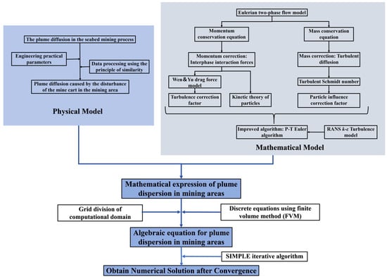
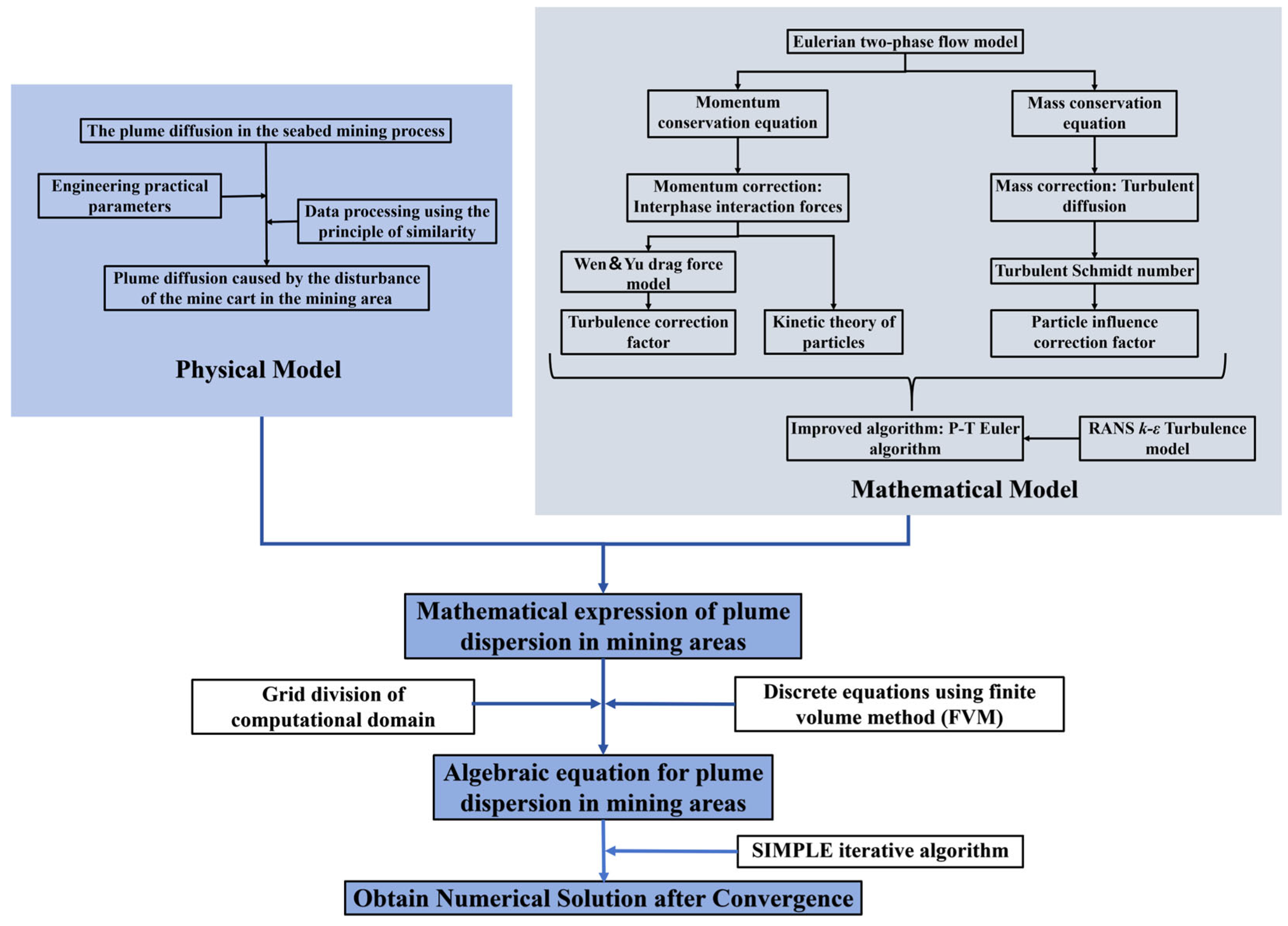
In summary, the numerical framework of this study discretizes the computational domain using the finite volume method (FVM) and iteratively solves the modified N-S equations using the SIMPLE algorithm, with the turbulence model being handled by the $k-\epsilon$ RANS model. The overall logic and algorithmic framework are illustrated in Figure 1. The numerical model employed in this study focuses on particle–fluid interactions (particularly between particles and turbulence) and particle–particle interactions, aiming to capture key characteristics of sediment plume dispersion in deep-sea mining. It should be noted as a limitation of the present study that flocculation effects are not considered. Although flocculation may influence particle settling under certain conditions, the current model focuses on primary particle dynamics and is considered suitable for the low-concentration, non-flocculant scenarios investigated.

Figure 1. Schematic of the logical and algorithmic framework of the paper.

2.2. Definition of Characteristic Scale

To better compare and analyze the flow at different practical scales that share common characteristic scale nodes, as well as to further investigate the flow mechanisms of fine-grained buoyant jets, we define characteristic scales related to distance, time, and velocity. These characteristic scales provide the theoretical foundation for subsequent dimensionless analysis. Specifically, these characteristic scales are derived from the volumetric flux and momentum flux of the injection source [53].

The expression for the volumetric flux of the source is:

$$Q_0={\displaystyle \frac{1}{{\rho }_p}}{\displaystyle \underset{A}{\int }{\rho }_{\mathrm{p}}{V}_j}dA$$

(32)

The expression for the momentum flux of the source is:

$$M_0={\displaystyle \frac{1}{{\rho }_p}}{\displaystyle \underset{A}{\int }{\rho }_{\mathrm{p}}{V}_j^2}dA$$

(33)

The expression for the characteristic length l_q in this study is:

$$l_q={\displaystyle \frac{Q_0}{M_0^{1/2}}}\sim L_m$$

(34)

The expression for the characteristic time t_q is:

$$t_q={\displaystyle \frac{Q_0^2}{M_0^{3/2}}}\sim L_m/V_m$$

(35)

The expression for the characteristic velocity v_q is:

$$v_q={\displaystyle \frac{M_0}{Q_0}}\sim V_m$$

(36)

In the subsequent discussion, we will nondimensionalize the corresponding dimensional quantities using the characteristic length l_q, characteristic time t_q, and characteristic velocity v_q.

2.3. Physical Model and Boundary Conditions

Liu et al. [11] summarized various parameters of deep-sea mining vehicles, as outlined by Sun et al. [54] and Yang et al. [55], which are presented in Table 1. As shown in the table, the average length of the deep-sea mining vehicles currently under development is approximately 5 m, with an average width of around 3 m. Additionally, a deep-sea mining vehicle capable of extracting 10,000 tons of polymetallic nodules per day will disturb approximately 40,000 tons of seabed sediment [56]. The sediment concentration within the plume generated by the mining vehicle ranges from 25 to 80 g/L [57]. Assuming an average sediment concentration of 52.5 g/L, the resulting turbidity current velocity is estimated at approximately 0.6 m/s. In comparison, the operational speed of the mining vehicle on the seabed is about 0.5 m/s [11]. This suggests that the sediment discharge velocity is of a similar order of magnitude to the vehicle’s movement speed. Furthermore, the seabed flow field, which is influenced by tidal forces, generates flow velocities on the centimeter scale [19,58]. Based on the engineering parameters of deep-sea mining operations, this study will employ a 1:100 scale ratio to conduct numerical simulations of the plume and its diffusion within a 30 × 30 m² mining area.

Table 1. Dimensional parameters of deep-sea mining vehicles [11].

Time (Year)	Research and Development Group	Geometric Parameter (Length × Width × Height)
1978	America/Ocean Minerals Corporation (OMCO)	3.415 × 2.44 × 2.1 m3
1999	Germany/University of Siegen	3.1 × 3.0 × 2.0 m3
1980	France/Vertut et al.	5.5 × 3.3 × 2.6 m3
1999	India/National Institute of Ocean Technology (NIOT)	3.16 × 2.95 × 2.5 m3
2001	China/Changsha Institute of Mining Research Co. (Changsha, China)	4.6 × 3.0 × 2.1 m3
2021	China/Marine Engineering Team of SJTU	5.0 × 2.5 × 2.1 m3

①

Geometric similarity

$${\displaystyle \frac{L}{L_m}}={\displaystyle \frac{l}{l_m}}={\displaystyle \frac{w}{w_m}}=100$$

(37)

where L represents the side length of the mining area, which is taken as 30 m; L_m is the side length of the scaled-down mining area model, calculated to be 0.3 m; l represents the length of the mining vehicle, taken as 5 m; l_m is the length of the scaled-down mining vehicle model, calculated to be 0.05 m; w represents the width of the mining vehicle, taken as 3 m; and w_m is the width of the scaled-down mining vehicle model, calculated to be 0.03 m.

②

Dynamics similarity of mining vehicle motion

$$Fr=V/\sqrt{gl}=V_m/\sqrt{g{l}_m}$$

(38)

where Fr represents the standard Froude number; V represents the actual speed of the mining vehicle, taken as 0.5 m/s; and V_m represents the speed of the mining vehicle in the scaled-down model, calculated to be 0.05 m/s.

In conclusion, this study involved an investigation of the actual engineering processes and derived the necessary data for the simulation based on geometric and kinematic similarity, as presented in Table 2. The particle size of the sediment was determined using the d₅₀ (the median particle diameter, denoted as d₅₀, is defined as the particle size at which 50% of the total volume of the sediment sample consists of particles with a diameter smaller than this value, based on the cumulative particle size distribution.) value for deep-sea sediment particles, which were collected from a depth of 5200 m in the Pacific mining area. This value, as measured by Zelin Liu et al. [59], was found to be 7.43 micrometers. Additionally, important parameters such as the density of the environmental fluids and the density of the sediment particles were established in accordance with the environmental context of deep-sea mining. The specific parameter settings are outlined in Table 2.

Table 2. Experimental data used in this study.

Parameter	Name	SI Unit	Range or Value
A	Length of the calculation domain	m	4
B	Width of the calculation domain	m	4
H	Height of the calculation domain	m	1
lm	Length of the mining vehicle	m	0.05
wm	Width of the mining vehicle	m	0.03
Lm	Side length of the mining area	m	0.3
Vm	Motion speed of the mining vehicle	m s−1	0.05
Vj	Turbidity current velocity generated by the mining vehicle	m s−1	0.025–0.1 (0.025, 0.05, 0.075, 0.1)
Va	Velocity of the ambient fluid	m s−1	0–0.1 (0, 0.025, 0.05, 0.075, 0.1)
ρf	Ambient fluid density	kg m−3	1030
μf	Ambient fluid viscosity	Pa s	0.001
ρs	Density of the sediment	kg m−3	2650
ρp	Injection term density	kg m−3	1062.4
μP	Injection fluid viscosity	Pa s	0.001
d	Particle diameter	m	7.43 × 10−6
αs	Particle phase volume fraction	1	0.02

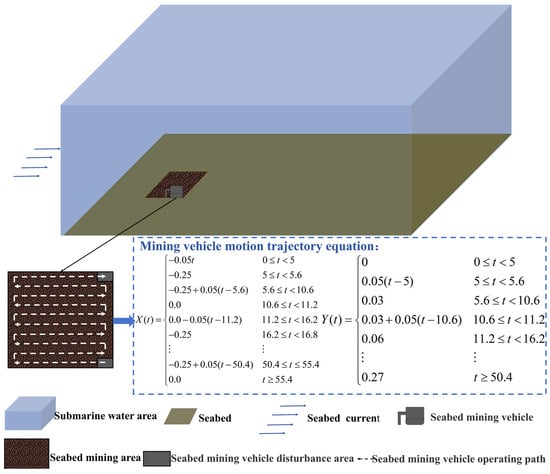
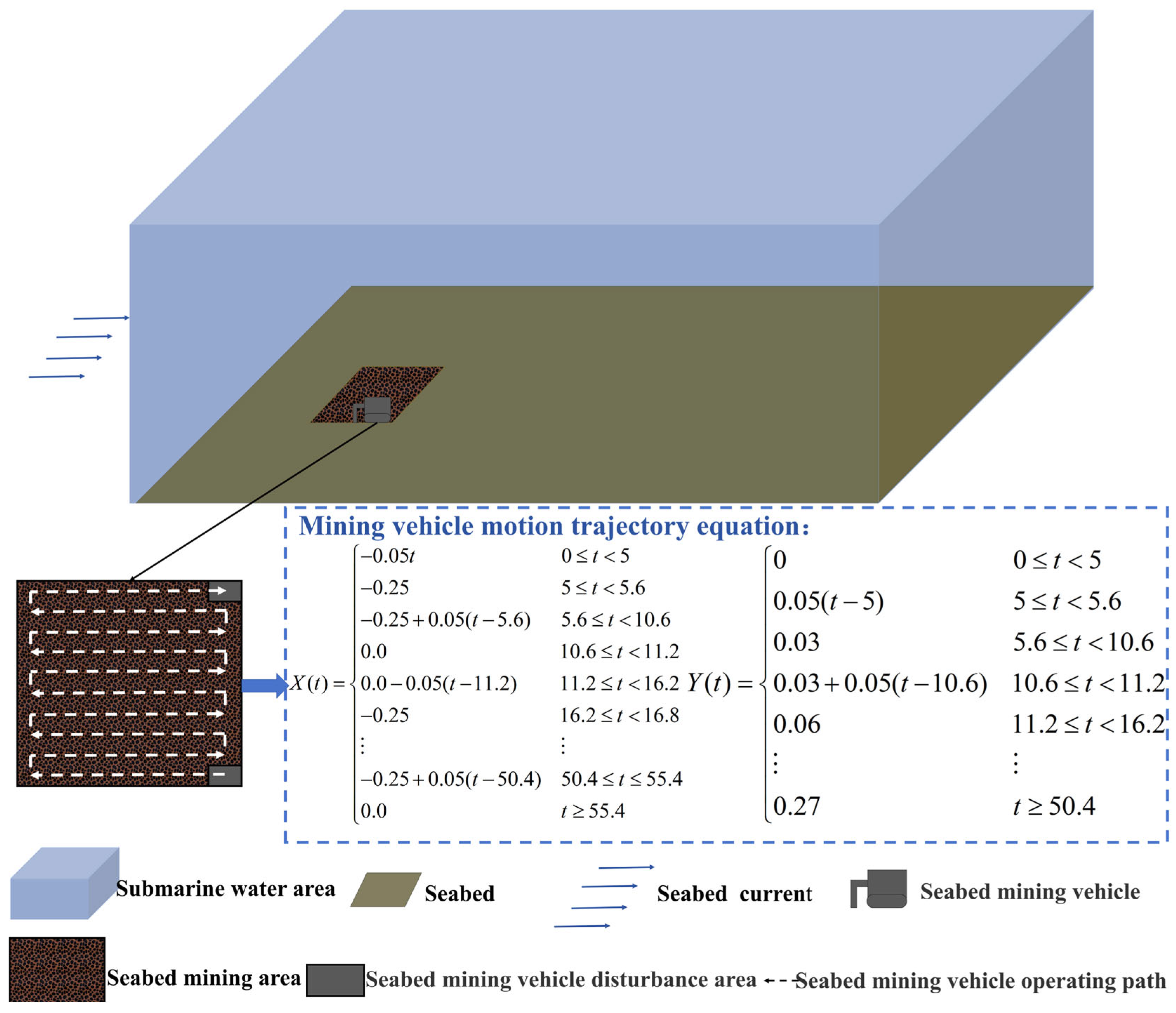
Based on these parameters, a computational model was developed to simulate the disturbance and pollution in the mining area during underwater mining activities. The model employed a rectangular computational domain, with the origin placed at the center of the mining vehicle’s initial position. Figure 2 illustrates the computational domain used in this study, and the corresponding motion trajectory equation for the mining vehicle is also defined here.

Figure 2. Computational model of this study.

To enhance the control of flow in the convective field, Table 3 summarizes all the key dimensionless numbers relevant to this study. Among these, the Atwood number (At) is less than 1 (At ≪ 1), which indicates that the experiment focuses on jets with small density differences, thus satisfying the Boussinesq approximation. The environmental fluid and the medium fluid of the turbulent flow are identical in this numerical simulation experiment, resulting in a viscosity ratio of m = 1. The Péclet number (Pe) was calculated and found to be much greater than 1 (Pe ≫ 1), suggesting that the effect of molecular diffusion on the numerical simulation experiment can be neglected. Additionally, the computational domain is sufficiently large (δ₁ >> 1, δ₂ >> 1, δ₃ >> 1), so boundary conditions have a negligible influence on the movement of the jet. As a result, the primary dimensionless parameters in this study include the Froude number (Fr), the dimensionless plume emission velocity (V_jn), and the dimensionless ambient fluid velocity (V_an). Since the sediment emission concentration is constant in this numerical simulation experiment, the Froude number (Fr) and the dimensionless plume emission velocity (V_jn) are linearly related. Consequently, the primary focus is placed on the influence of the dimensionless plume emission velocity (V_jn, range: 0.5–2) and the dimensionless ambient fluid velocity (V_an, range: 0–2).

Table 3. Main dimensionless parameters defining the plume flow field of mining activities in the mining area.

Parameter	Name	Definition	Range or Value
At	Atwood number	${\displaystyle \frac{{\rho }_p-{\rho }_f}{{\rho }_p+{\rho }_f}}$	0.015
Frp	Froude number for plume	${\displaystyle \frac{V_j}{\sqrt{Atg{w}_m}}}$	0.38–1.51
m	Viscosity ratio	${\displaystyle \frac{{\mu }_f}{{\mu }_p}}$	1
Pe	Péclet number	${\displaystyle \frac{V_j{w}_m}{2\times {10}^{-9}}}$	(0.375–1.5) × 106
Vjn	Dimensionless plume emission velocity	${\displaystyle \frac{V_j}{V_m}}$	785–3139
Van	Dimensionless ambient fluid velocity	${\displaystyle \frac{V_a}{V_m}}$	0–2
δ1	Aspect ratio 1	${\displaystyle \frac{A}{w_m}}$	133.3
δ2	Aspect ratio 2	${\displaystyle \frac{B}{w_m}}$	133.3
δ3	Aspect ratio 3	${\displaystyle \frac{H}{w_m}}$	33.33
αs	Particle phase volume fraction	${\displaystyle \frac{V{f}_s}{Vf}}$	0.02

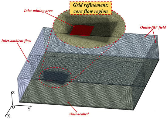
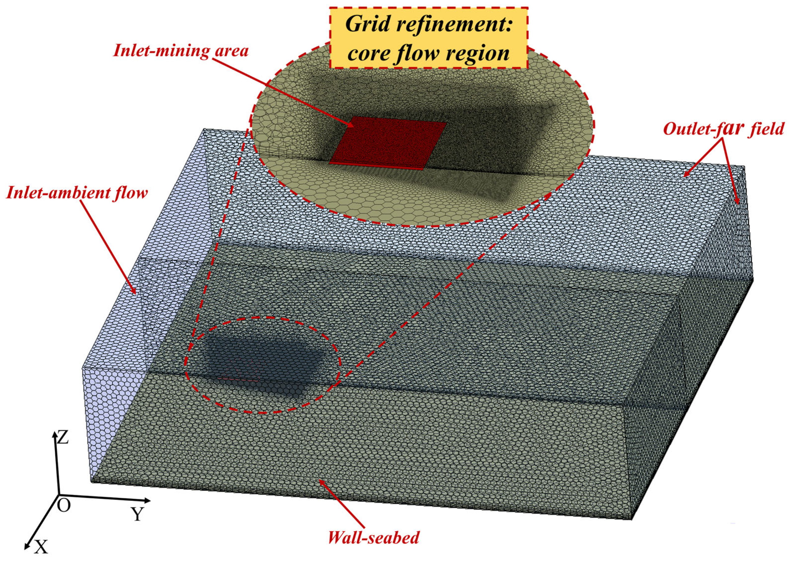
The grid required for the finite volume method calculations was established through grid partitioning. We defined the inlet-ambient flow to control the velocity of the ambient and background fluids, simulating the bottom current velocity. The mining area was designated as the inlet-mining area, and the speed variation within this area was adjusted to simulate the disturbance caused by the movement of the mining vehicle on the seabed. Additionally, a grid refinement zone, labeled “Grid Refinement: Core Flow Region,” was implemented near the inlet-mining area to more precisely capture the detailed flow field after the plume is generated in the mining area. This refinement ensured computational accuracy and allowed for better resolution of flow details in the critical region near the mining area, which is the focus of our observation. The influence of the seabed on the flow field was modeled as a wall–seabed boundary condition, with surrounding areas defined as pressure outlets. Given that the computational domain is sufficiently large, the effect of the outlet boundary can be neglected. To accurately capture the influence of the seabed (wall–seabed), five boundary layers were established, and the Menter–Lechner wall function was applied. For more detailed information on the Menter–Lechner wall function, please refer to Kamaci and Kaya [60] and Luo [61]. The final grid partitioning model is shown in Figure 3. All subsequent analyses in this study were conducted within a Cartesian coordinate system, where the directions of each axis adhered to the coordinate system defined in Figure 3.

Figure 3. Grid computational model.

2.4. Grid Convergence Analysis and Model Validation

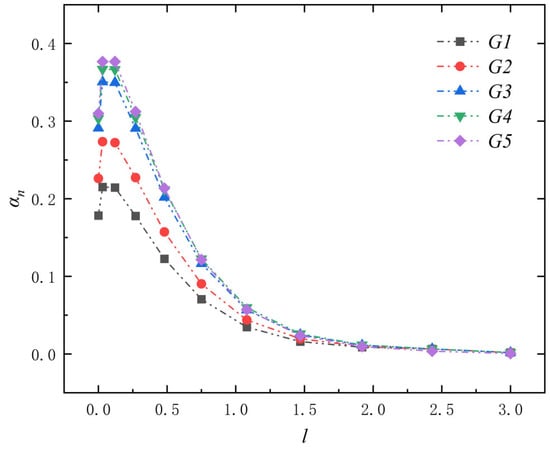
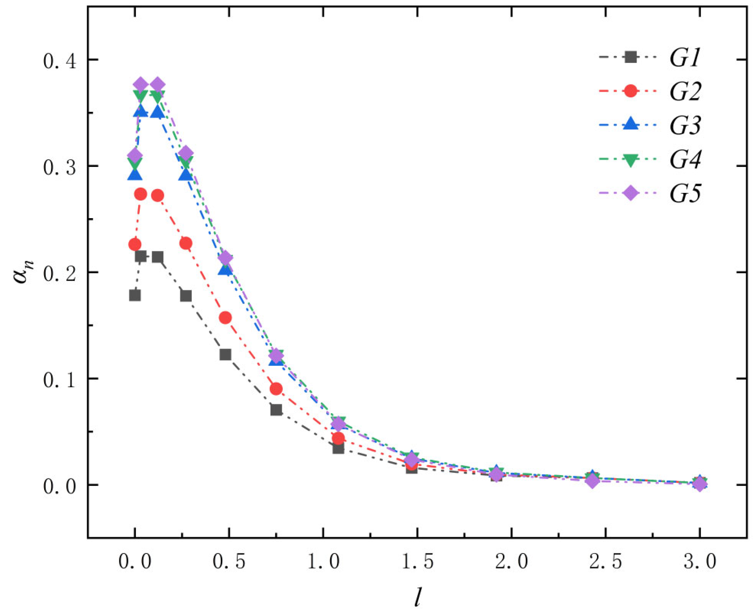
In numerical experiments, the grid resolution is critical for the accuracy of the results. To assess its impact, we tested five different grid resolution scenarios, as presented in Table 4. These simulations were conducted under the conditions of a mining vehicle-induced turbidity current with a velocity of V_jn = 1 and a background flow velocity of V_an = 0. We monitored the relative volume fraction of the particle phase along the diagonal line 1w_m above the mining area, defined as α_n = α_l/α_s, where αl represents the local volume fraction of the solid phase in the flow field. The results are presented in Figure 4. As shown in Figure 4, the relative volume fraction of the particle phase gradually stabilizes as the number of grids increases from G1 to G5. Notably, the grid number increases by approximately 16% between G4 and G5, yet the results remain almost identical. This suggests that the G4 grid resolution offers sufficient accuracy for the simulation while also optimizing computational resource usage; consequently, for the subsequent numerical calculations, we will adopt the G4 grid resolution.

Table 4. Grid resolution conditions.

Index	G1	G2	G3	G4	G5
Mesh Number	2,131,821	3,290,169	6,788,674	8,798,425	10,225,619

Figure 4. Distribution of relative volume fraction in the flow field along the diagonal line at 1w_m above the mining area (where l is the ratio of the actual distance to the width of the mining vehicle) under different grid resolutions.

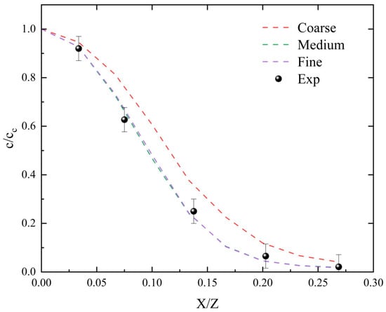
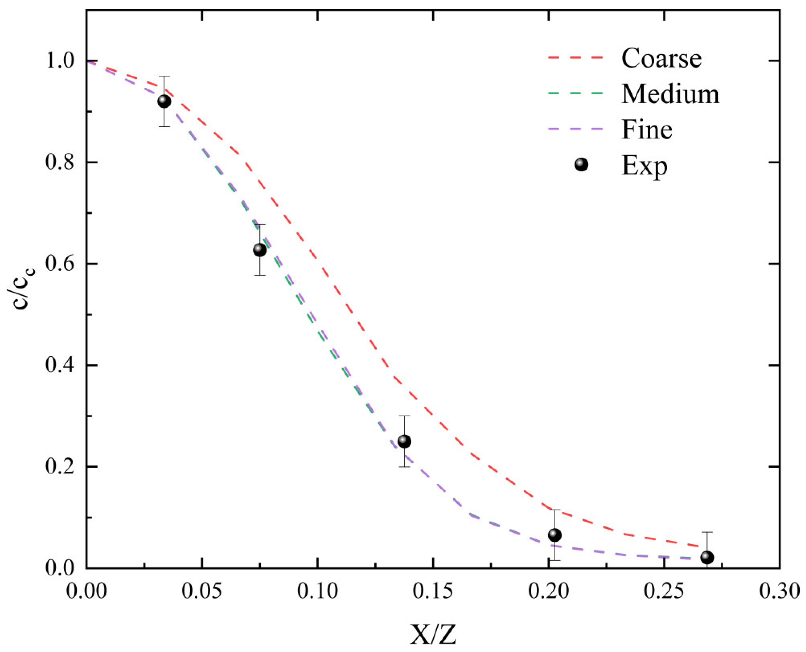
To further validate the accuracy of our numerical model, we adopted the experimental framework developed by Decrop et al. [15]. This model focuses on the vertical discharge of particle phase concentration near the wall, differing from our constructed model in the direction of particle phase emission. However, experimental studies on seafloor transport are relatively scarce, making it difficult to obtain stable and reliable validation data; therefore, we selected an experimental scenario with more abundant data and stronger verifiability. This choice was made based on the high consistency of the physical problems between our numerical scenario and the experimental scenario, as the primary interaction forces within the physical fields that they focus on are key aspects, such as particle–fluid interactions, particle–particle collisions and friction, and particle transport characteristics within the flow field. Through this comparative validation, the accuracy of the numerical methods employed in this study can be demonstrated concisely and convincingly. For the numerical simulations, we used the framework outlined in Figure 1, ensuring that the simulation conditions mirrored those of the experiments in the literature (V_j = 0.12 m/s, α_s = 0.0019). Simulations were performed with grids of low, medium, and high resolutions. We then analyzed the distribution of the relative volume fraction along the x-axis at Z = 9D, comparing it to the volume fraction at the axis. Furthermore, we superimposed the experimental results from Decrop et al. [15] onto the figure, as shown in Figure 5. The results show that when the grid resolution is set to medium or high, the numerical calculations stabilize, with errors remaining within 5% when compared to the experimental data. These findings confirm that the numerical model we have employed is both accurate and effective for simulating plume diffusion in deep-sea mining areas.

Figure 5. Validation of numerical framework accuracy: comparison between numerical method and experimental results from Decrop et al. [15]—distribution of dimensionless concentration along the x/z-axis at Z = 9D.

To better discuss the impact of the dimensionless plume emission velocity V_jn and the dimensionless ambient fluid velocity V_an on plume diffusion in the mining area, we studied 20 condition combinations shown in Table 5 and defined the representation of these conditions for subsequent discussion. In this notation, A, B, C, and D represent the dimensionless plume emission velocity V_jn, and 1, 2, 3, 4, and 5 represent the dimensionless ambient fluid velocity V_an.

Table 5. Operating conditions of this study.

Van Vjn	0.5/A	1.0/B	1.5/C	2.0/D
0.0/1	Case A1	Case B1	Case C1	Case D1
0.5/2	Case A2	Case B2	Case C2	Case D2
1.0/3	Case A3	Case B3	Case C3	Case D3
1.5/4	Case A4	Case B4	Case C4	Case D4
2.0/5	Case A5	Case B5	Case C5	Case D5

3. Results and Discussion

3.1. Spatial Diffusion of the Plume

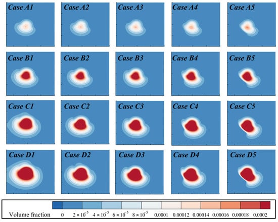
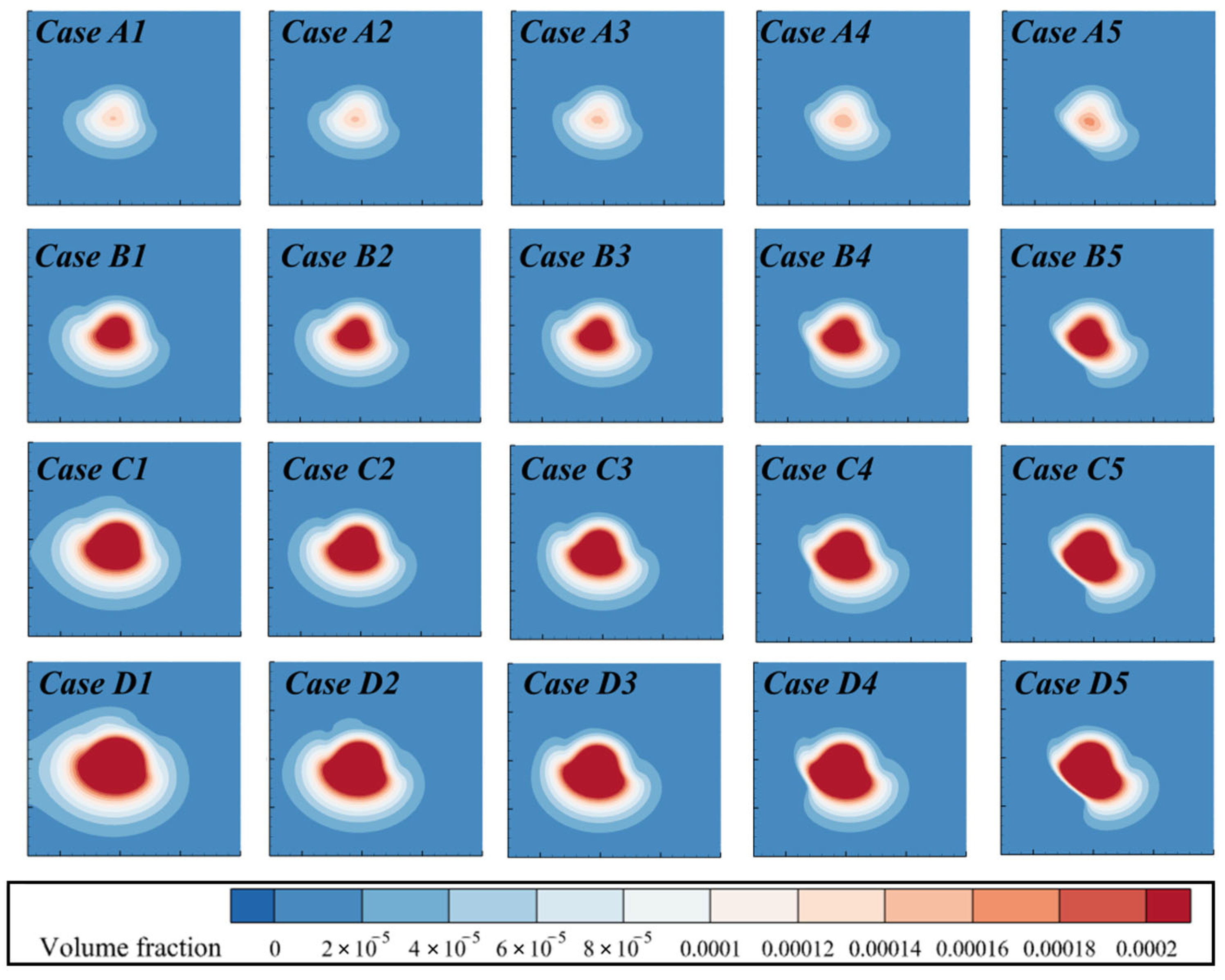
Figure 6 presents the concentration contour plots of the plume at a dimensionless distance of 1 from the top of the mining area under varying conditions of dimensionless plume emission velocity and dimensionless ambient fluid velocity. As depicted, the high-concentration core of the plume remains concentrated at the top of the mining area. With an increase in the dimensionless ambient fluid velocity, the changes in the diffusion pattern of the plume exhibit a similar trend across different conditions of dimensionless plume emission velocity; specifically, the flow and transport effects of the surrounding fluid cause the plume to diffuse in the direction of the flow (i.e., along the positive x-axis). This is observed as a receding of the left side of the plume inward along the positive X-direction, while the right side extends outward in the same direction. Additionally, as the dimensionless plume emission velocity increases, the overall diffusion range of the plume expands under all ambient fluid velocity conditions.

Figure 6. Contour plots of particle phase volume concentration distributions at the top of the mining area (Z = 1ln) under different operating conditions.

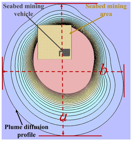
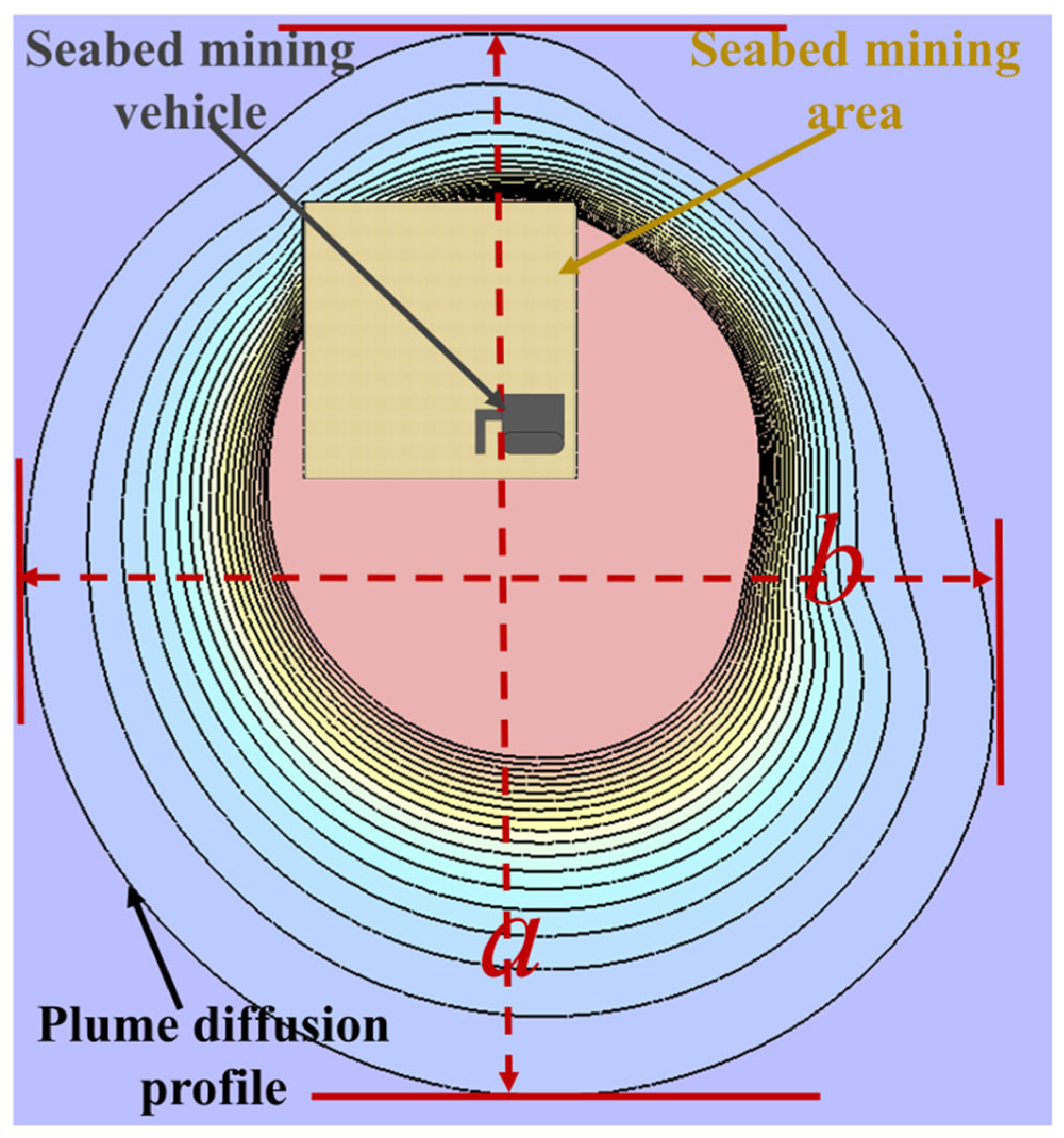
To further investigate the spatial diffusion of the plume, we employed the method illustrated in Figure 7 to measure the length a and width b of the plume’s outermost edge in the XY-plane under various operating conditions. The dimensionless equivalent area for each scenario was subsequently calculated using Equation (39) as follows:

$$A_e=\pi {((a/l_q+b/l_q)/4)}^2$$

(39)

Figure 7. Schematic diagram of plume diffusion range in the mining area.

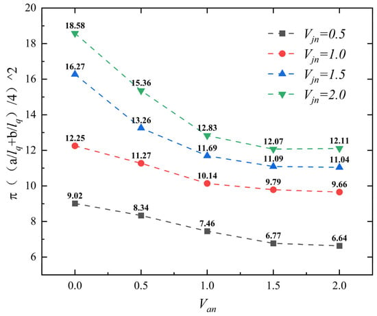
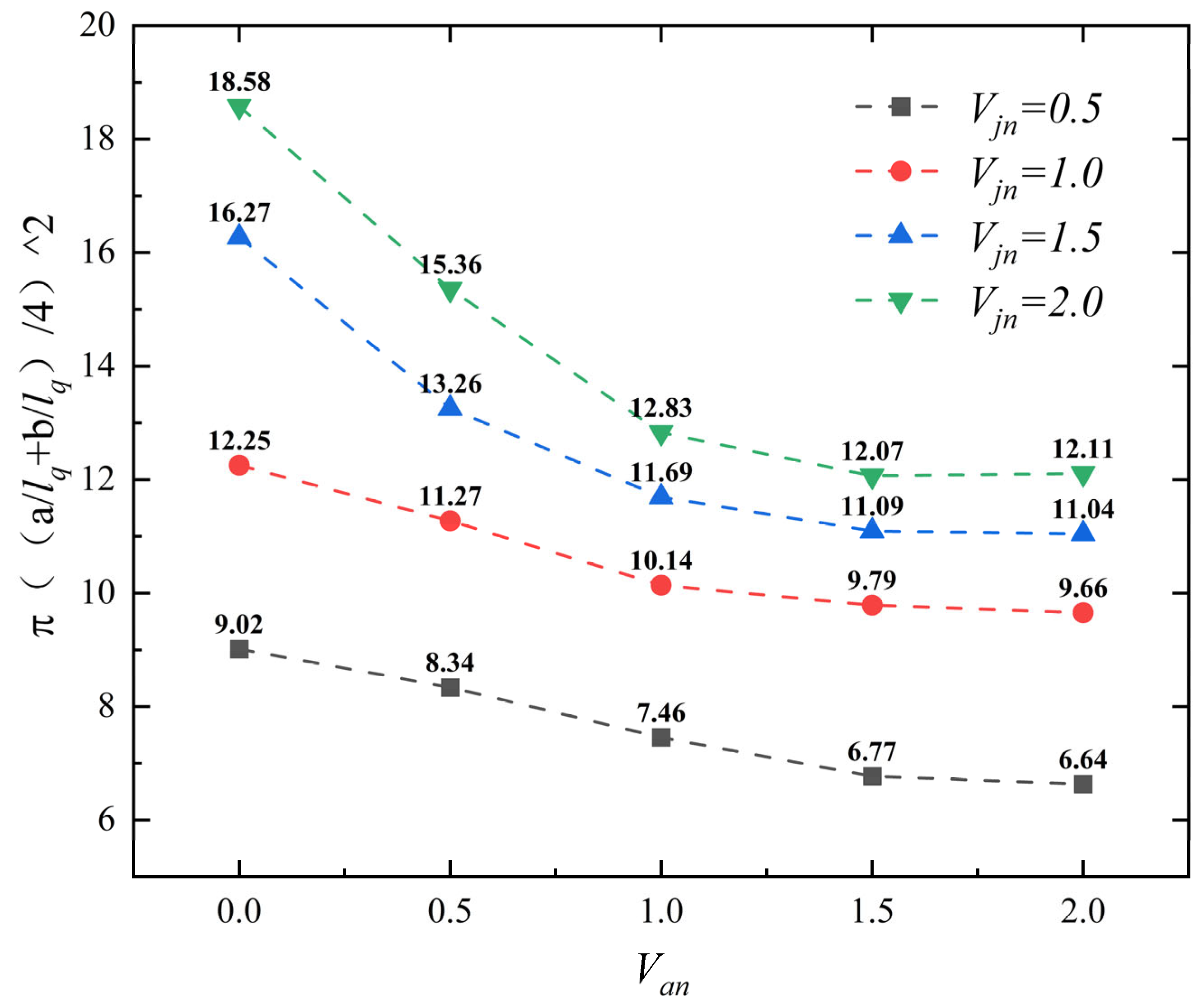
From Figure 8, it is evident that as the dimensionless plume emission velocity increases, the dimensionless equivalent area of the plume consistently exhibits a marked increase under different dimensionless ambient fluid velocity conditions. Conversely, as the dimensionless ambient fluid velocity increases, the dimensionless equivalent area tends to decrease, regardless of the dimensionless plume emission velocity.

Figure 8. Variation in dimensionless equivalent area under different operating conditions as a function of dimensionless ambient fluid velocity (V_an).

Specifically, when V_an = 0 (no ambient flow), the dimensionless equivalent area increases from 9.02 to 18.58 as V_jn increases from 0.5 to 2.0, corresponding to an increase of approximately 106%. At V_an = 0.5, the dimensionless equivalent area increases from 8.34 to 15.36 under the same V_jn range, representing an increase of about 48%. At V_an = 1.0, the dimensionless equivalent area increases from 7.46 to 12.83, an increase of approximately 72%. At V_an = 1.5, it increases from 6.77 to 12.07, an increase of about 78%. At V_an = 2.0, it increases from 6.64 to 12.11, corresponding to an increase of approximately 82%.

Furthermore, when V_jn = 0.5, the dimensionless equivalent area decreases from 9.02 to 6.64 as V_an increases from 0 to 2.0, a reduction of about 26%. At V_jn = 1.0, it decreases from 12.25 to 9.66, a reduction of approximately 21%. At V_jn = 1.5, it decreases from 16.27 to 11.04, a reduction of about 32%. At V_jn = 2.0, it decreases from 18.58 to 12.11, a reduction of approximately 35%.

In summary, with increasing dimensionless plume emission velocity, the dimensionless equivalent area increases by up to 106%, while with increasing dimensionless ambient fluid velocity, it decreases by up to 35%.

The observed trends can be attributed to the distinct roles of the two controlling parameters. The increase in dimensionless equivalent area with higher emission velocity reflects the direct contribution of enhanced sediment turbidity volume flux, which enlarges the diffusion range. In contrast, the reduction in the equivalent area with increasing ambient flow velocity is due to the enhanced upward transport and downstream advection of the plume, which shift sediment away from the bottom XY-plane; thus, emission velocity primarily governs the extent of diffusion, while ambient flow velocity controls the stretching and deflection of the diffusion morphology.

In summary, the spatial diffusion of the plume at the top of the mining area is jointly governed by the dimensionless emission velocity and the ambient flow velocity. An increase in emission velocity significantly enlarges the dimensionless equivalent area of the plume, reflecting the direct contribution of enhanced sediment turbidity flux to the diffusion range. Conversely, an increase in ambient flow velocity markedly reduces the equivalent area by promoting upward transport and downstream advection of the plume. The roles of the two factors in spatial diffusion are clearly differentiated: emission velocity dictates the extent of diffusion, while ambient flow velocity governs the stretching and deflection of the diffusion morphology.

3.2. Effect of Ambient Flow Velocity on the Temporal Process of Plume in Mining Areas

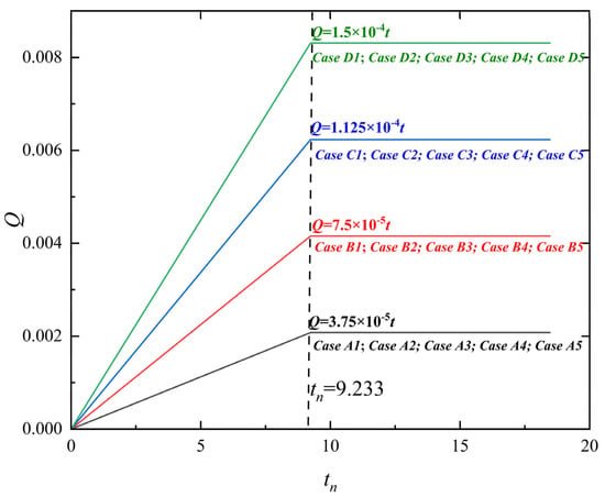
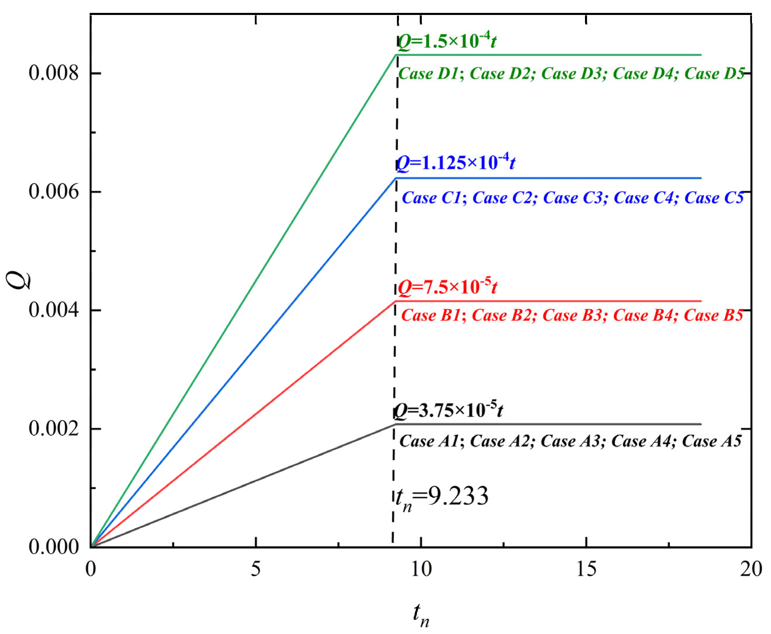
Figure 9 illustrates the temporal evolution of the sediment turbidity volume flux of the plume in the mining area, providing a visual representation of the disturbance process shown in Figure 2. The total dimensionless simulation time is 18.167 t_q. Mining-induced disturbance ceases at t_n = 9.233 t_q, the mining disturbance concludes, and the plume diffusion shifts from being influenced by both mining disturbance and environmental transport to a process predominantly driven by environmental transport. Building on the analysis from the previous section, we observe that under different dimensionless plume emission velocity conditions, the spatial distribution characteristics of the plume follow similar trends. Therefore, in this section, we focus on a dimensionless plume emission velocity of V_jn = 1.0 as a representative case to further explore the impact of mining disturbance on the temporal dynamics of plume diffusion.

Figure 9. Cumulative volume flux of disturbed plume in the mining area with time (where t_n denotes the time scale normalized by t_q).

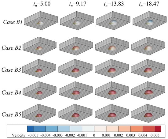
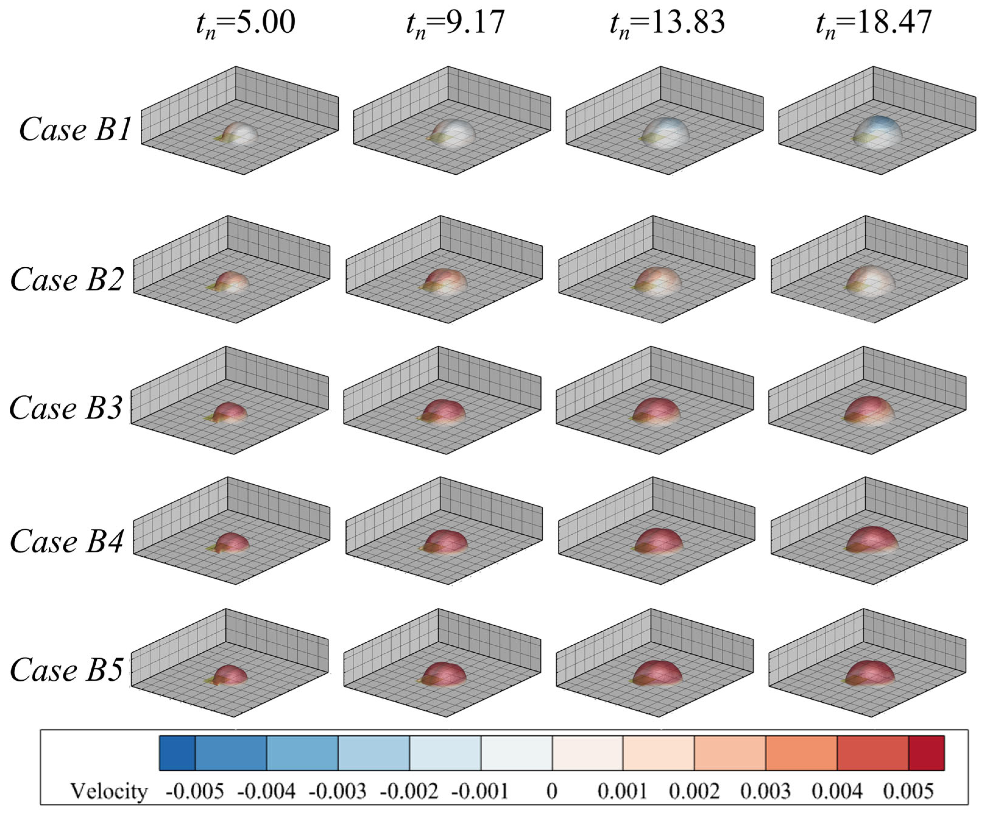
Figure 10 presents contour plots showing the coupling of the outer edge of the plume’s core region (α_s = 0.0002) with the velocity in the Z-direction, as the dimensionless ambient fluid velocity increases under fixed V_jn = 1.0. During the period t_n = 9.17 to 18.47, as the sediment turbidity volume flux stabilizes, the outer edge of the plume’s core region gradually extends outward. As the dimensionless ambient fluid velocity increases, the X-direction velocity at the outer edge of the plume’s core region exhibits a consistent upward trend over time. Under Case B1 (V_an = 0.0, no ambient flow), the X-direction velocity at the outer edge shows a significant negative value region, indicating substantial settlement. When the dimensionless ambient fluid velocity increases to V_an = 0.5 to 2.0 (Cases B2–B5), the X-direction velocity becomes predominantly positive.

Figure 10. Morphological evolution of plume under different environmental flow velocities.

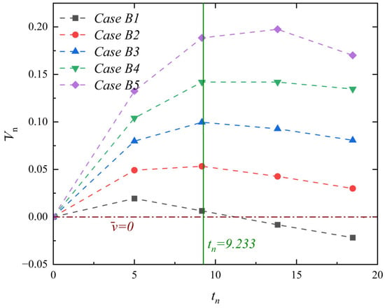
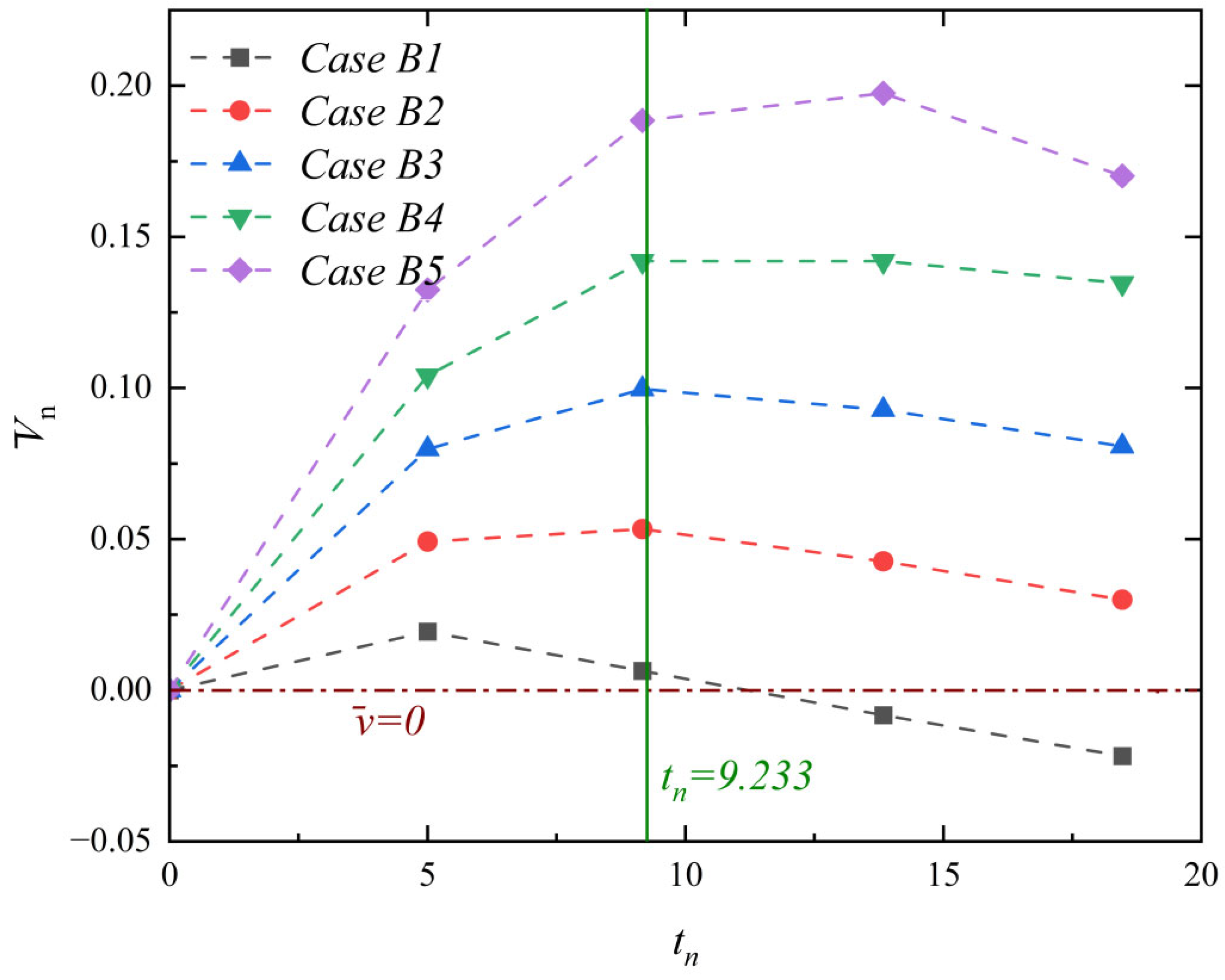
To further quantify the settling behavior, Figure 11 presents the variation in the dimensionless mean velocity in the Z-direction at the outer edge of the plume’s core region (α_s = 0.0002) as V_an increases, with V_jn = 1.0. As the ambient flow intensifies, the dimensionless mean Z-direction velocity increases markedly. Under Case B1, once mining disturbance ceases, the dimensionless velocity mean rapidly drops below zero, indicating entry into a settling state. Under all scenarios with an ambient flow (Cases B2–B5), the dimensionless velocity mean consistently remains above 1 throughout the process. The combined effects of mining disturbance and ambient transport (for t_n ≤ 9.233) result in a gradual increase in Z-direction velocity over time, while after disturbance ceases (t_n > 9.233), the Z-direction velocity gradually decreases.

Figure 11. Time variation curve of average settling velocity at the plume edge (where t_n denotes the time scale normalized by t_q).

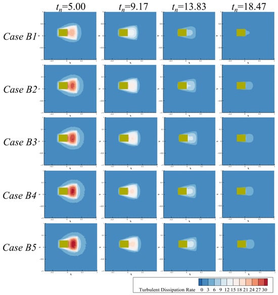
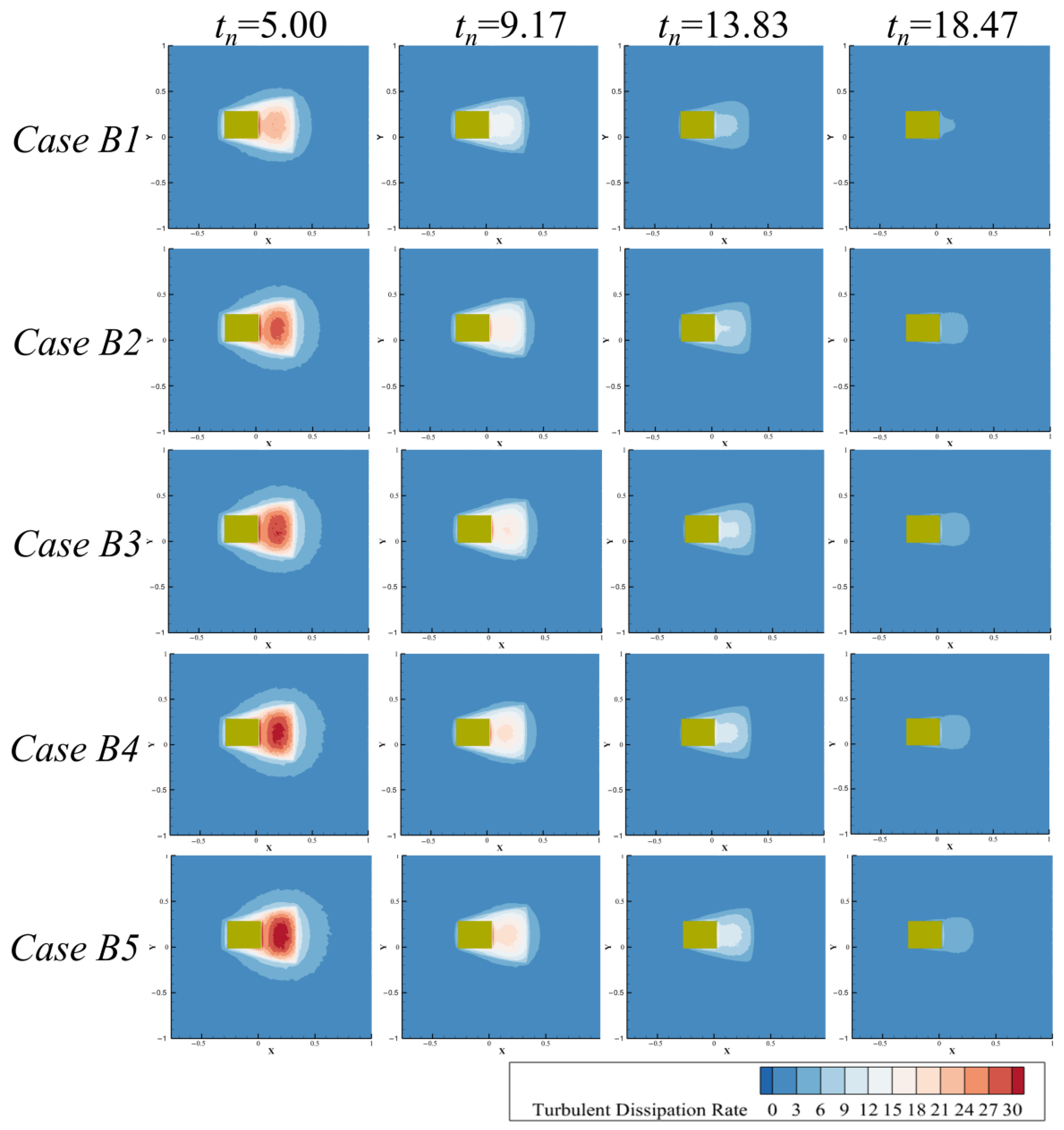
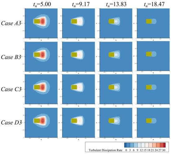
Figure 12 demonstrates the variation in the turbulent dissipation rate in the XY-plane of the flow field with changes in V_an, under a fixed V_jn = 1.0. As plume diffusion progresses over time, the turbulent dissipation rate at the bottom plane decreases gradually under different conditions. At all times, as V_an increases, the turbulent dissipation rate in the XY-plane increases significantly.

Figure 12. Turbulent dissipation rate of the flow field under different environmental flow velocities.

These results indicate that the ambient flow velocity is the dominant factor controlling the temporal evolution of the plume. Under constant emission velocity, increased ambient flow suppresses the settling of the plume’s core region, driving its continuous outward expansion in both vertical and horizontal directions. The elevated turbulent dissipation rate under stronger ambient flow accelerates plume transport toward the far field. In the absence of an ambient flow, the plume rapidly settles after the cessation of disturbance. In contrast, when an ambient flow is present, the plume’s core region maintains a sustained upward migration trend, demonstrating that the ambient flow plays a dominant role during the later stage of plume evolution.

3.3. Impact of Mining Disturbance on the Temporal Process of Plume in Mining Areas

In the previous section, we observed that the spatial distribution characteristics of the plume exhibit significant similarity under varying dimensionless ambient fluid velocities. Building on this observation, we now focus on a dimensionless ambient fluid velocity of V_an = 1.0 as a representative condition to further investigate the temporal characteristics of plume diffusion in the presence of a mining area disturbance.

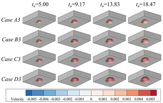
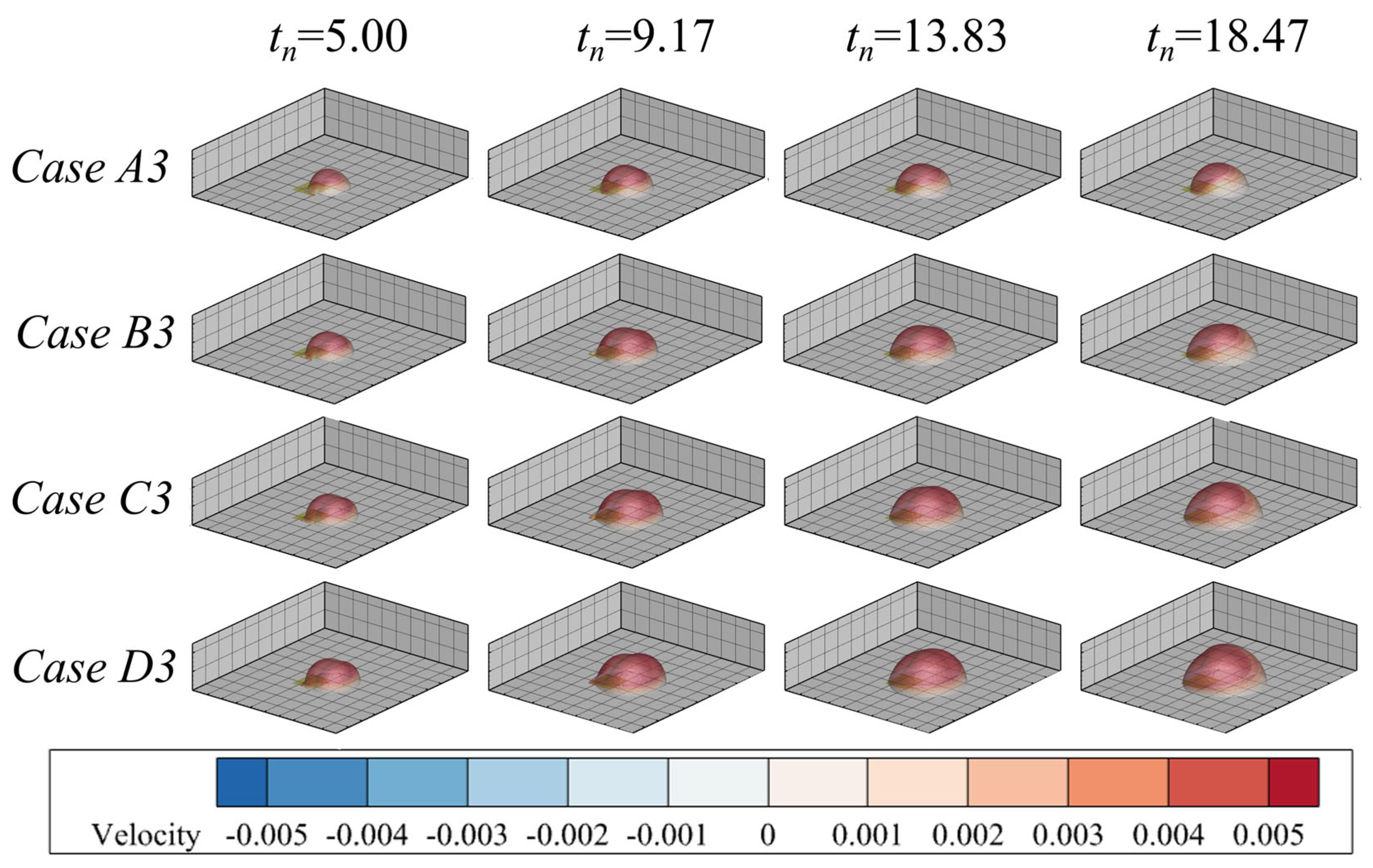
Figure 13 illustrates coupled contour plots of the plume’s core region outer edge (α_s = 0.0002) and Z-direction velocity, as the dimensionless plume emission velocity increases under a fixed V_an = 1.0. Under V_an = 1.0, the plume gradually spreads outward over time. For different dimensionless plume emission velocities, the contour of the plume’s core region consistently shows progressive expansion during the observed temporal process. As the dimensionless plume emission velocity increases, the turbidity flux of the plume increases, leading to continuous widening of the diffusion range.

Figure 13. Morphological evolution of plume under different jet velocities.

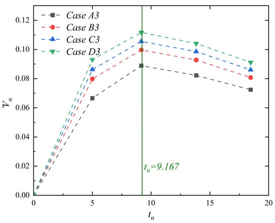
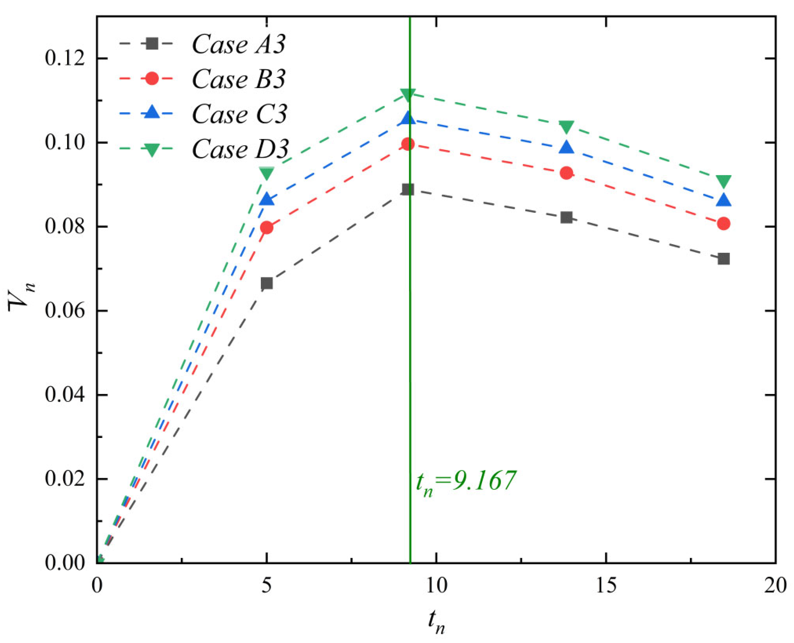
To further quantify the impact of emission velocity on plume diffusion, Figure 14 presents the variation in the dimensionless mean Z-direction velocity at the outer edge of the plume’s core region (α_s = 0.0002) as V_jn increases, with a fixed V_an = 1.0. The dimensionless mean Z-direction velocity increases progressively as V_jn rises across all observed time steps. The temporal variation trend remains consistent across different V_jn conditions, displaying an initial increase followed by a decrease. After the mining disturbance concludes (t_n > 9.167), the dimensionless mean Z-direction velocity begins to decline immediately.

Figure 14. Time variation curve of the average settling velocity at the plume edge (where t_n denotes the time scale normalized by t_q).

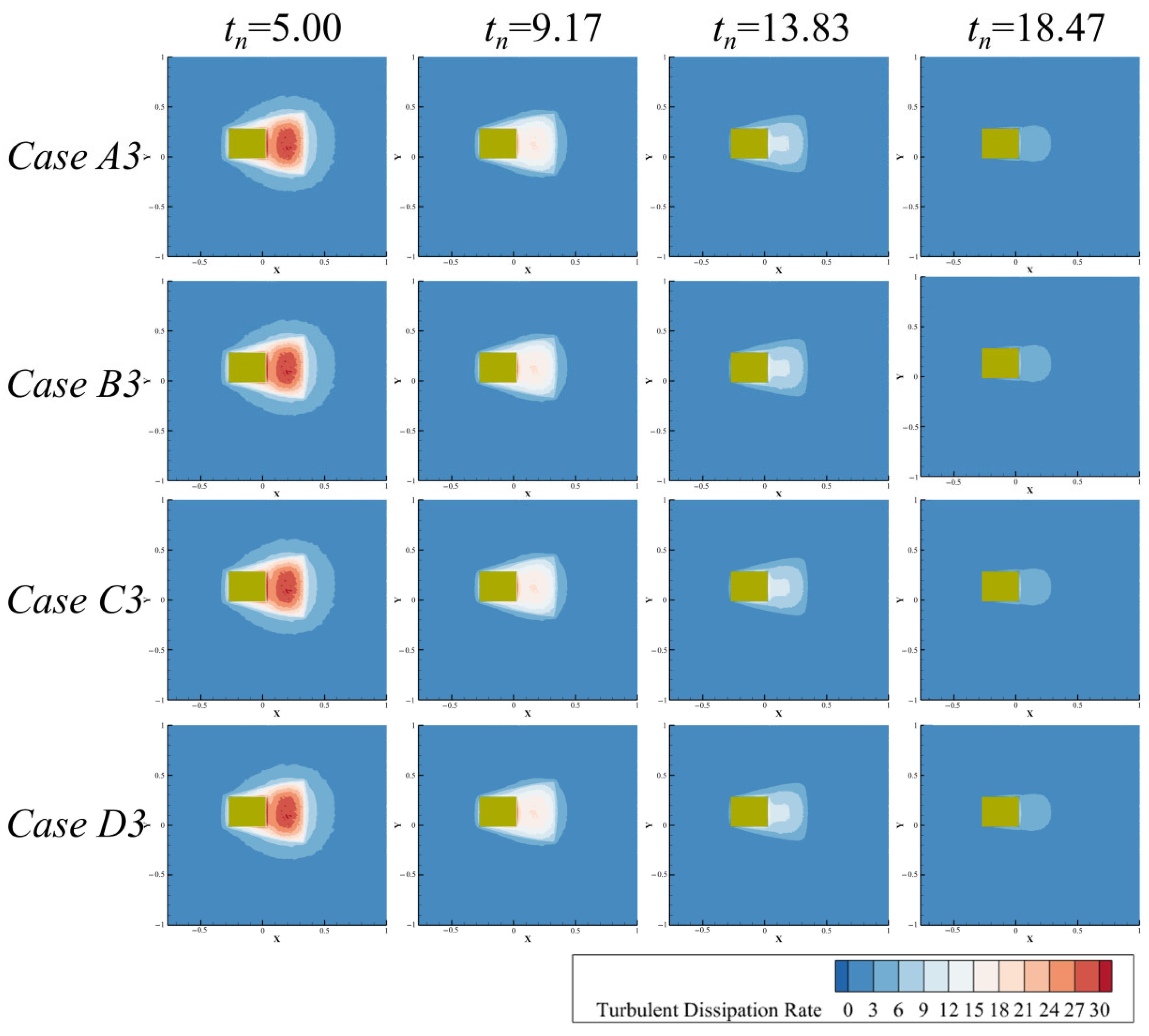
Figure 15 illustrates the variation in the turbulent dissipation rate in the XY-plane with changes in V_jn, under a fixed V_an = 1.0. Across all time steps, the turbulent dissipation rate remains largely unaffected by changes in the dimensionless plume emission velocity.

Figure 15. Turbulent dissipation rate of the flow field under different jet velocities.

These results indicate that, under constant ambient flow velocity, the intensity of mining disturbance, represented by the dimensionless emission velocity, significantly influences the temporal evolution of the plume. As the emission velocity increases, the diffusion range of the plume’s core region expands continuously, settling behavior is inhibited, and vertical migration velocity increases markedly. However, variations in the emission velocity have a limited effect on the turbulent dissipation rate within the flow field, suggesting that the enhancement of plume diffusion is primarily achieved through an increased sediment flux rather than by altering the turbulent transport structure of the flow field. After the cessation of mining disturbance, the diffusion trend of the plume’s core region remains influenced by the disturbance intensity, indicating that the emission velocity plays a dominant role during the early and middle stages of plume evolution.

4. Conclusions

This study employed a validated P-T Euler modeling framework based on the similarity principle to integrate sediment disturbance induced by polymetallic nodule mining vehicles with ambient current effects, thereby enabling a systematic investigation of near-field plume generation and far-field dispersion processes in polymetallic nodule mining areas. The findings have revealed the hydrodynamic mechanisms governing the behavior of mining-induced sediment plumes, providing new insights into this field.

The plume emission velocity primarily governed the turbidity flux and the resulting spatial extent of the plume. Increasing the dimensionless emission velocity significantly enlarged the diffusion range of the plume core due to the associated increase in sediment volume flux. Under certain ambient flow conditions, higher emission velocities can also delay particle settling, allowing suspended sediments to remain entrained within the plume for longer periods. As a result, the disturbance generated by mining activities became the dominant driver controlling plume spreading within the mining area.

The ambient fluid velocity controlled the transport pathway and spatial morphology of the plume. An increase in the dimensionless ambient velocity substantially modified plume advection, promoting downstream transport and extending the plume toward the far field. This behavior was reflected by the reduction in the dimensionless equivalent area projected on the seabed plane and the enhanced vertical transport velocity at the plume boundary. Consequently, stronger ambient currents facilitated plume dispersion and increased the spatial influence of suspended sediments.

The results further indicated that the ambient flow velocity and plume emission velocity affected plume dynamics through distinct mechanisms. Increasing the ambient velocity intensified turbulent dissipation within the flow field, which enhanced mixing and governed the ultimate spatial distribution of suspended sediments. In contrast, increasing the plume emission velocity primarily increased the initial turbidity flux while exerting limited influence on the intrinsic turbulent transport characteristics of the flow field. Therefore, plume expansion under higher emission velocities mainly resulted from the increased sediment input rather than from changes in the turbulence structure. Quantitatively, as the dimensionless plume emission velocity (V_jn) increased from 0.5 to 2.0, the dimensionless equivalent area—a key indicator of the plume’s spatial footprint—increased by up to 106%. Conversely, as the dimensionless ambient fluid velocity (V_an) increased from 0 to 2.0, the dimensionless equivalent area decreased by up to 35%, reflecting the enhanced upward transport and downstream advection that shifted sediment away from the seabed.

From an environmental perspective, the simulated turbulent dissipation rate serves as a critical link between physical dispersion and benthic habitat disturbance. Under increasing ambient current velocities, the near-bed turbulent dissipation rate increased by approximately one order of magnitude. This intensified mechanical disturbance, combined with elevated suspended sediment concentrations—and the associated reduction in near-bed plume footprint by up to 35%—may affect feeding efficiency, larval settlement, and community structure in deep-sea ecosystems. These findings highlight the coupled roles of emission intensity and ambient hydrodynamic conditions in determining the spatial influence of mining-induced sediment plumes.

A key challenge in environmental management is establishing sediment impact thresholds for various benthic species. This study provides a simple, physically based reference by quantifying key variables that govern disturbance intensity—including local concentration, turbulent dissipation rate, plume residence time, and sedimentation flux. However, further research is needed to deepen understanding in this area so that these physical simulation results can be integrated with biological impact thresholds (for example, existing studies [4,20,21]) to develop a coupled physical–ecological assessment framework. Such an effort would provide a comprehensive reference for the formulation of environmental assessment standards for deep-sea mining and thereby advance the commercialization of deep-sea mining technologies.

References

- Yang, L.; Luo, L.; Chen, X.; Wu, X.; Jing, F. Hydraulic Transportation of Non-Spherical Coarse Particles in Deep-Sea Mining: Impact of Particle Shape on Flow Dynamics. Ocean. Eng. 2025, 323, 120652. [Google Scholar] [CrossRef] [Scilit]
- Zhang, Q.; Chen, X.; Luan, L.; Sha, F.; Liu, X. Technology and Equipment of Deep-Sea Mining: State of the Art and Perspectives. Earth Energy Sci. 2025, 1, 65–84. [Google Scholar] [CrossRef] [Scilit]
- Hu, J.; Jin, G.; Zou, L.; Yu, Z.; Dong, X.; Qian, H. Solid–Liquid Two-Phase Flow Characteristics Considering Nonspherical Mineral Particles in Deep-Sea Mining Systems. Ocean. Eng. 2025, 320, 120323. [Google Scholar] [CrossRef] [Scilit]
- Larsen, O.; Banks, A.; van Berkel, J.J.; Clarke, M.; Elsasser, B.; Foster, T. Monitoring and Modeling of Deep-Water Sediment Plumes from Deep-Sea Mining. In Deep-Sea Mining Management, Policy and Regulation: Data Management, Environmental Monitoring, Techno-Economic Assessment, Law of the Sea and Regulatory Regimes; Sharma, R., Ed.; Springer Nature: Cham, Switzerland, 2025; pp. 325–358. ISBN 978-3-031-92737-9. [Google Scholar]
- Singh, P.A.; Jaeckel, A.; Ardron, J.A. A Pause or Moratorium for Deep Seabed Mining in the Area? The Legal Basis, Potential Pathways, and Possible Policy Implications. Ocean. Dev. Int. Law 2025, 56, 18–44. [Google Scholar] [CrossRef] [Scilit]
- Xu, L.; Li, X.; Liu, Y.; Dou, P.; Hong, Z.; Han, C. A Review of Plume Research in the Collection Process of Deep-Sea Polymetallic Nodules. Water 2024, 16, 3379. [Google Scholar] [CrossRef] [Scilit]
- Ali, S.H. Deep-Sea Mining Opponents: There’s No Free Lunch When It Comes to Clean Energy. Nature 2024, 626, 480. [Google Scholar] [CrossRef] [Scilit]
- Ouillon, R.; Kakoutas, C.; Meiburg, E.; Peacock, T. Gravity Currents from Moving Sources. J. Fluid Mech. 2021, 924, A43. [Google Scholar] [CrossRef] [Scilit]
- Ouillon, R.; Muñoz-Royo, C.; Alford, M.H.; Peacock, T. Advection–Diffusion Settling of Deep-Sea Mining Sediment Plumes. Part 2. Collector Plumes. Flow 2022, 2, E23. [Google Scholar] [CrossRef] [Scilit]
- Liu, S.; Yang, J.; Lu, H.; Sun, P.; Zhang, B. A Numerical Investigation of the Dynamic Interaction between the Deep-Sea Mining Vehicle and Sediment Plumes Based on a Small-Scale Analysis. J. Mar. Sci. Eng. 2023, 11, 1458. [Google Scholar] [CrossRef] [Scilit]
- Liu, S.; Yang, J.; Lyu, H.; Sun, P.; Zhang, B. Experimental and Numerical Investigation of the Effect of Deep-Sea Mining Vehicles on the Discharge Plumes. Phys. Fluids 2024, 36, 033358. [Google Scholar] [CrossRef] [Scilit]
- Liu, G.; Liu, L. Numerical simulation of fine particle plume flow in deep-sea mining. Ocean. Eng. 2023, 41, 150–160. [Google Scholar] [CrossRef]
- Yang, Y.; Chen, J.; Wang, Y. Particle Plume Dispersion with Various Incident Velocities: Particle–Fluid Interaction Regimes from Coupled Discrete Element-Large Eddy Simulations. Phys. Fluids 2024, 36, 083318. [Google Scholar] [CrossRef] [Scilit]
- Bai, T.; Zhao, Y.; Zhou, Y.; Huang, K. Numerical Simulation and Analysis of Initial Plume Discharge of Deep-Sea Mining. Ocean. Eng. 2024, 310, 118794. [Google Scholar] [CrossRef] [Scilit]
- Decrop, B.; De Mulder, T.; Toorman, E.; Sas, M. New Methods for ADV Measurements of Turbulent Sediment Fluxes—Application to a Fine Sediment Plume. J. Hydraul. Res. 2015, 53, 317–331. [Google Scholar] [CrossRef] [Scilit]
- Byishimo, P. Experiments and 3D CFD Simulations of Deep-Sea Mining Plume Dispersion and Seabed Interactions. Master’s Thesis, Technische Universiteit Delft, Delft, The Netherlands, 2018. [Google Scholar]
- Wijmans, Y.R. Horizontal Negatively Buoyant Jets in Deep Sea Mining. Master’s Thesis, Technische Universiteit Delft, Delft, The Netherlands, 2021. [Google Scholar]
- Liu, S.; Yang, J.; Lyu, H.; Sun, P.; Zhang, B. A Numerical Investigation of the Effects of Deep-Sea Mining Vehicles on the Evolution of Sediment Plumes Based on the Combination of near- and Far-Field Models. Appl. Ocean. Res. 2024, 149, 104048. [Google Scholar] [CrossRef] [Scilit]
- Purkiani, K.; Gillard, B.; Paul, A.; Haeckel, M.; Haalboom, S.; Greinert, J.; de Stigter, H.; Hollstein, M.; Baeye, M.; Vink, A.; et al. Numerical Simulation of Deep-Sea Sediment Transport Induced by a Dredge Experiment in the Northeastern Pacific Ocean. Front. Mar. Sci. 2021, 8, 719463. [Google Scholar] [CrossRef] [Scilit]
- Muñoz-Royo, C.; Ouillon, R.; El Mousadik, S.; Alford, M.H.; Peacock, T. An in Situ Study of Abyssal Turbidity-Current Sediment Plumes Generated by a Deep Seabed Polymetallic Nodule Mining Preprototype Collector Vehicle. Sci. Adv. 2022, 8, eabn1219. [Google Scholar] [CrossRef] [Scilit]
- Muñoz-Royo, C.; Peacock, T.; Alford, M.H.; Smith, J.A.; Le Boyer, A.; Kulkarni, C.S.; Lermusiaux, P.F.J.; Haley, P.J.; Mirabito, C.; Wang, D.; et al. Extent of Impact of Deep-Sea Nodule Mining Midwater Plumes Is Influenced by Sediment Loading, Turbulence and Thresholds. Commun. Earth Environ. 2021, 2, 148. [Google Scholar] [CrossRef] [Scilit]
- Spearman, J.; Taylor, J.; Crossouard, N.; Cooper, A.; Turnbull, M.; Manning, A.; Lee, M.; Murton, B. Measurement and Modelling of Deep Sea Sediment Plumes and Implications for Deep Sea Mining. Sci. Rep. 2020, 10, 5075. [Google Scholar] [CrossRef] [Scilit]
- Van Reeuwijk, M.; Salizzoni, P.; Hunt, G.R.; Craske, J. Turbulent Transport and Entrainment in Jets and Plumes: A DNS Study. Phys. Rev. Fluids 2016, 1, 074301. [Google Scholar] [CrossRef] [Scilit]
- Shi, D.-P.; Luo, Z.-H.; Zheng, Z.-W. Numerical Simulation of Liquid–Solid Two-Phase Flow in a Tubular Loop Polymerization Reactor. Powder Technol. 2010, 198, 135–143. [Google Scholar] [CrossRef] [Scilit]
- Qiaoqun, S.; Huilin, L.; Wentie, L.; Yurong, H.; Lidan, Y.; Gidaspow, D. Simulation and Experiment of Segregating/Mixing of Rice Husk–Sand Mixture in a Bubbling Fluidized Bed. Fuel 2005, 84, 1739–1748. [Google Scholar] [CrossRef] [Scilit]
- Huilin, L.; Yurong, H.; Wentie, L.; Ding, J.; Gidaspow, D.; Bouillard, J. Computer Simulations of Gas–Solid Flow in Spouted Beds Using Kinetic–Frictional Stress Model of Granular Flow. Chem. Eng. Sci. 2004, 59, 865–878. [Google Scholar] [CrossRef] [Scilit]
- Shi, P.; Sommer, A.E.; Rox, H.; Eckert, K.; Rzehak, R. Euler-Euler/RANS Modeling of Solid-Liquid Flow in Stirred Tanks: A Comprehensive Model Validation. Miner. Eng. 2022, 185, 107679. [Google Scholar] [CrossRef] [Scilit]
- Wu, W.M.; Wang, S.Y. Mathematical Models for Liquid-Solid Two-Phase Flow. Int. J. Sediment Res. 2000, 15, 288–298. [Google Scholar]
- Zhang, Z.C.; Li, Y.P.; Zhang, L.J.; Chen, D.X. Drag Force Modification Model for Turbulent Suspended-Load Sediment Solid-Liquid Two-Phase Flow. J. Fluids Struct. 2023, 118, 103861. [Google Scholar] [CrossRef] [Scilit]
- Zhang, Y.; Li, Y.; Zhu, Z.; Cui, B. Computational Analysis of Centrifugal Pump Delivering Solid-Liquid Two-Phase Flow during Startup Period. Chin. J. Mech. Eng. 2014, 27, 178–185. [Google Scholar] [CrossRef] [Scilit]
- Nguyen, Y.; Wells, J.; Truong, H. Fictitious-domain simulation of solid-liquid flow with “subgrid” lubrication force correction; A sphere falling onto a plane surface. Proc. Hydraul. Eng. 2007, 51, 151–156. [Google Scholar] [CrossRef] [Scilit]
- Wang, S.; Guo, S.; Gao, J.; Lan, X.; Dong, Q.; Li, X. Simulation of Flow Behavior of Liquid and Particles in a Liquid–Solid Fluidized Bed. Powder Technol. 2012, 224, 365–373. [Google Scholar] [CrossRef] [Scilit]
- Enwald, H.; Peirano, E.; Almstedt, A.E.; Leckner, B. Simulation of the Fluid Dynamics of a Bubbling Fluidized Bed. Experimental Validation of the Two-Fluid Model and Evaluation of a Parallel Multiblock Solver. Chem. Eng. Sci. 1999, 54, 311–328. [Google Scholar] [CrossRef] [Scilit]
- Peirano, E.; Palchonok, G.; Johnsson, F.; Leckner, B. Estimates of Turbulence Mechanisms in Circulating Fluidized Bed Combustors. Powder Technol. 1998, 96, 90–105. [Google Scholar] [CrossRef] [Scilit]
- Wen, C.Y.; Yu, Y.H. Mechanics of Fluidization. Chem. Eng. Prog. Symp. Ser. 1966, 62, 100–111. [Google Scholar]
- Yang, M. Two-Phase Flow CD Simulations and its Study. Master’s Thesis, Tianjin University, Tianjin, China, 2006. [Google Scholar]
- Clift, R.; Gauvin, W.H. Motion of Entrained Particles in Gas Streams. Can. J. Chem. Eng. 1971, 49, 439–448. [Google Scholar] [CrossRef] [Scilit]
- Brucato, A.; Grisafi, F.; Montante, G. Particle Drag Coefficients in Turbulent Fluids. Chem. Eng. Sci. 1998, 53, 3295–3314. [Google Scholar] [CrossRef] [Scilit]
- Zarin, N.A.; Arthur Nicholls, J. Sphere Drag in Solid Rockets—Non-Continuum and Turbulence Effects. Combust. Sci. Technol. 1971, 3, 273–285. [Google Scholar] [CrossRef] [Scilit]
- Gidaspow, D. Multiphase Flow and Fluidization: Continuum and Kinetic Theory Description. J. Non-Newton. Fluid Mech. 1994, 55, 207–208. [Google Scholar] [CrossRef] [Scilit]
- Ding, J.; Gidaspow, D. A Bubbling Fluidization Model Using Kinetic Theory of Granular Flow. AIChE J. 1990, 36, 523–538. [Google Scholar] [CrossRef] [Scilit]
- Chapman, S.; Cowling, T.G. The Mathematical Theory of Non-Uniform Gases. Math. Gaz. 1939, 23, 488–489. [Google Scholar] [CrossRef] [Scilit]
- Simonin, O.; Viollet, P.L. Modelling of Turbulent Two-Phase Jets Loaded with Discrete Particles. Phenom. Multiph. Flow 1990, 259–269. [Google Scholar]
- Shao, X.; Xia, Z. Stochastic Theory of Suspended Particle Distribution in Turbulent Flow Fields. Acta Mech. Sin. 1991, 28–36. Available online: https://kns.cnki.net/kcms2/article/abstract?v=Vs3rztogjcXeM2LR0cYa2ItWKhcfv82pSxN-BO3Eyx__LTXEHivdmeY_mTeccuLUJ3W0IhaEwuGYtmOOCEUYy97ox3x2nJy3L3kpkVx1jL3GeeMaLKllAkCrRcdFYLv_vh_AQfeiFgJkzmVwpATqcwDFHXquNuWD7hQ446Ai7nkxReq5-X1J1A==&uniplatform=NZKPT&language=CHS (accessed on 1 April 2026).
- Sokolichin, A.; Eigenberger, G.; Lapin, A. Simulation of Buoyancy Driven Bubbly Flow: Established Simplifications and Open Questions. AIChE J. 2004, 50, 24–45. [Google Scholar] [CrossRef] [Scilit]
- Shao, X.; Xia, Z. Stochastic Analysis of Turbulent Diffusion Coefficient of Suspended Particles. J. Hydraul. Eng. 1990, 32–40. Available online: https://kns.cnki.net/kcms2/article/abstract?v=Vs3rztogjcWXw1mdXNPlypNqET0rPP5XJb36EhQF2jbD7gCBz-KsKQKQ_O1bNTSFBSiGwPZcI-jwCq-7bfyQ21TSou0BtpMP8dg4YcmekMcjbNsxj2lkGw5O7arwCrhn3xzLwJJZ5cdCaC75LKUKK-kqaj54v3Bc5luOqxCQeTjj9maMcUYleQ==&uniplatform=NZKPT&language=CHS (accessed on 1 April 2026).
- Feng, X.; Cheng, J.; Li, X.; Yang, C.; Mao, Z.S. Numerical Simulation of Turbulent Flow in a Baffled Stirred Tank with an Explicit Algebraic Stress Model. Chem. Eng. Sci. 2012, 91, 30–44. [Google Scholar] [CrossRef] [Scilit]
- Lew, A.J.; Buscaglia, G.C.; Carrica, P.M. A Note on the Numerical Treatment of the K-Epsilon Turbulence Model. Int. J. Comput. Fluid Dyn. 2001, 14, 201–209. [Google Scholar] [CrossRef] [Scilit]
- Guozhi, Z.; Fanrang, K.; Jingchun, Z.; Zhiwei, Z.; Hua, C. Numerical Simulation of Turbulent Flow Field Based on SIMPLE Algorithm. Water Resour. Power 2007, 97, 100–102. [Google Scholar]
- Moukalled, F.; Mangani, L.; Darwish, M. The Finite Volume Mesh in OpenFOAM® and uFVM. In The Finite Volume Method in Computational Fluid Dynamics: An Advanced Introduction with OpenFOAM® and Matlab; Moukalled, F., Mangani, L., Darwish, M., Eds.; Springer International Publishing: Cham, Switzerland, 2016; pp. 173–207. ISBN 978-3-319-16874-6. [Google Scholar]
- Pawar, S.; San, O. CFD Julia: A Learning Module Structuring an Introductory Course on Computational Fluid Dynamics. Fluids 2019, 4, 159. [Google Scholar] [CrossRef] [Scilit]
- Qin, J.; Pan, H.; Rahman, M.M.; Tian, X.; Zhu, Z. Introducing Compressibility with SIMPLE Algorithm. Math. Comput. Simul. 2021, 180, 328–353. [Google Scholar] [CrossRef] [Scilit]
- Hassanzadeh, H.; Taghavi, S.M. A Review on Free Miscible Buoyant Jets. Phys. Fluids 2024, 36, 061301. [Google Scholar] [CrossRef] [Scilit]
- Sun, P.; Lu, H.; Yang, J.; Liu, M.; Li, S.; Zhang, B. Numerical Study on Shear Interaction between the Track Plate of Deep-Sea Mining Vehicle and the Seafloor Sediment Based on CEL Method. Ocean. Eng. 2022, 266, 112785. [Google Scholar] [CrossRef] [Scilit]
- Yang, J.; Liu, L.; Lv, H.; Lin, Z. Deep-Sea Mining Equipment in China: Current Status and Prospect. Strateg. Study CAE 2020, 22, 1–9. [Google Scholar] [CrossRef] [Scilit]
- Sharma, R. Environmental Issues of Deep-Sea Mining. Procedia Earth Planet. Sci. 2015, 11, 204–211. [Google Scholar] [CrossRef] [Scilit]
- Sha, F.; Xi, M.; Chen, X.; Liu, X.; Niu, H.; Zuo, Y. A Recent Review on Multi-Physics Coupling between Deep-Sea Mining Equipment and Marine Sediment. Ocean. Eng. 2023, 276, 114229. [Google Scholar] [CrossRef] [Scilit]
- Peacock, T.; Ouillon, R. The Fluid Mechanics of Deep-Sea Mining. Annu. Rev. Fluid Mech. 2023, 55, 403–430. [Google Scholar] [CrossRef] [Scilit]
- Liu, Z.; Wu, X.; Rao, Q.; Yi, W.; Chen, S.; Zheng, H. Diffusion Characteristics of Deep-Sea Mining Sediment Plumes in Flowing Water by Large-Scale Water Tank Experiments. Trans. Nonferrous Met. Soc. China 2025, 35, 2747–2761. [Google Scholar] [CrossRef] [Scilit]
- Kamaci, C.; Kaya, K. Numerical Investigation of Aerodynamic Properties of Ahmed Body for Different Rear Slanted Surface Configurations. Eur. J. Sci. Technol. 2021, 28, 469–475. [Google Scholar] [CrossRef] [Scilit]
- Luo, H.; Zhang, C.; Zhu, J. Development of a Numerical Model for the Hydrodynamics Simulation of Liquid-Solid Circulating Fluidized Beds. Powder Technol. 2019, 348, 93–104. [Google Scholar] [CrossRef] [Scilit]
Disclaimer/Publisher’s Note: The statements, opinions and data contained in all publications are solely those of the individual author(s) and contributor(s) and not of MDPI and/or the editor(s). MDPI and/or the editor(s) disclaim responsibility for any injury to people or property resulting from any ideas, methods, instructions or products referred to in the content. |
© 2026 by the authors. Licensee MDPI, Basel, Switzerland. This article is an open access article distributed under the terms and conditions of the Creative Commons Attribution (CC BY) license.